
The Underground Railroad UNDERGROUND RAILROAD UNDERGROUND RAILROAD.
Preliminary Draft Comments Welcome
Are underground markets really more violent? Evidence from early 20th century America
Emily Greene Owens
Cornell University [email protected]
October 20091
Abstract
Over two thirds of the social harm associated with drug use is attributed to systemic violence in drug trafficking. The violent nature of drug markets is often cited as a rational for legalizing and regulating the sale of currently illegal narcotics. Further, an increase in crime during the 1920s, when alcohol sales were outlawed, is regularly presented as evidence that introducing formal dispute resolution into drug markets would reduce the total social cost of drug use. I test the theory that systemic violence is the primary cause of drug related crime by exploiting the fact that temperance laws were in place in over 30 states prior to Federal Prohibition, and remained in place in four states after Federal Prohibition was repealed. I also take advantage of the fact that the data set used to measure crime prior to 1933 is an unbalanced state level panel. I find support for the theory that underground markets are violent; in particular support for the “wet” cause was positively associated with homicides when temperance laws were in place. However, in contrast to prevailing wisdom, I find that on net, murder rates did not increase when alcohol markets were criminalized. Instead, the observed trends in crime are primarily explained by urbanization and immigration. My results suggest that the assertion that crime will fall if drug markets are legalized is not warranted. JEL codes: K42, N42 Keywords: Illegal markets, Alcohol regulation
1 I would like to thank George Boyer, Matthew Freedman, and William White for helpful discussion, as well as Michael Shores for outstanding research assistance. All errors are my own.
2
I. Introduction:
Lack of access to formal dispute resolution via the court system is frequently cited
as the underlying reason for the violent nature of illegal markets. Inductive reasoning
and observational evidence clearly support this claim. Legal economic transactions are
disputed frequently; in 2006, 13.6 million civil cases were filed in limited and general
jurisdiction state courts in the United States.2 In the absence of a court system, the
claimants in these cases would be limited in their ability to resolve their disputes, and one
of the remaining options available would be the use of physical force or intimidation
[Blumstein (1995)]. Consistent with this, illegal markets, especially illegal markets for
intoxicating substances, are characterized by high levels of violence [MacCoun and
Reuter (1998)]. However, the violence that we observe in modern-day illegal markets
can have non-institutional causes as well. Mind altering substances can increase the
likelihood that a user commits a violent crime, and individuals may engage in violent
crimes to acquire money to obtain the illegal good. Whether or not the legalization of
market for products like cocaine, heroin or marijuana is socially beneficial public policy
depends on the relative importance of “systemic” violence, violence resulting from the
fact that the market transactions themselves are illegal, as opposed to “economic-
compulsive” or “psychopharmacologic” reasons.3 Unfortunately, lack of substantial
variation in the legality of street drugs makes it difficult to predict the relative
contributions of these three mechanisms.
2 National Center for State Courts Court Statistics Project http://www.ncsconline.org/D_Research/csp/2007_files/2007_state_court_trial_sheets.html 3 These labels are taken from Goldstein (1985) who is credited with developing this three-part framework for thinking about the connection between drugs and crime.
3
In this paper I attempt to estimate the amount of violence associated with lack of
formal contract enforcement in markets by examining murder rates in the United States
between 1900 and 1936. Over the course of this time period, 32 state laws criminalized
the sale of alcohol, and in 1920 all alcohol sales and production were banned by the 18th
amendment of the US Constitution. Using state level variation in homicides, suicides,
accidental shootings, and “external” mortality rates, I find no evidence that driving the
alcohol market underground substantively increased the rate of violence in the US. I find
weak evidence that the passage of “bone dry” legislation (outright prohibition), including
the 18th amendment, had a net negative effect on the homicide rate, which is likely due to
decreased alcohol consumption in those states. Instead of alcohol temperance, much of
the observed trends in homicide rates during the early 20th century can be explained by
the urbanization of the population.
While this is contrary to established conventional wisdom regarding the effects of
temperance, my findings do not wholly contradict economic theory; using voting records
for state anti-alcohol laws and state ratification of the 18th amendment as a proxy for
demand for alcohol, and the fraction of states under temperance laws as a proxy for the
price of alcohol, I find that the areas which experienced the largest reductions in
homicides after outlawing alcohol likely had the lowest demand for the good. From a
policy standpoint, however, this finding casts doubt on the assertion that legalizing the
sale of illicit substances would necessarily lead to a reduction in crime. Theoretically, the
effect is ambiguous. Market illegality should lead to higher prices, which should reduce
psychopharmacological crime, but potentially increase economic-compulsive crime and,
most importantly, lead systemic violence. Empirically, I find that even without formal
4
contract enforcement, existing data provide no evidence that individuals used lethal force
to resolve disputes over alcohol on a large enough scale outweigh the reduction in
psychopharmacological violence.
The paper proceeds as follows: In the next section I summarize the existing
literature linking temperance, alcohol consumption, and violent crime. In section III I lay
out my analytic framework for testing the effect of market legality on crime, and describe
the data used to estimate this model in section IV. I present my empirical estimates in
section V. In order to fully test for any evidence that temperance laws affect homicide, I
replicate my primary analysis with four alternate measures of violence in section VI.
Finally, I conclude with discussion in section VII.
II. Temperance, Alcohol Consumption, and Violent Crime:
The combined passage of the 18th amendment and the Volstead Act, hereafter
“Federal Prohibition,” banned the manufacture, sale, and transportation of alcohol in the
United States.4 The enactment of Federal Prohibition in 1920 was the culmination of a
nearly century-long social movement in the US which pitted the “drys,” lead by groups
such as the Women’s Christian Temperance Union and Anti-Saloon League, against the
“wets,” financially supported by United States Brewers’ Association. This social
movement can be roughly classified into three waves; first, in the 1850s, 13 states
adopted laws restricting the use and local sale of alcohol, a move considered potentially
4 Section one of the 18th amendment, which was ratified in January of 1919, states that “After one year from the ratification of this article the manufacture, sale, or transportation of intoxicating liquors within, the importation thereof into, or the exportation thereof from the United States and all territory subject to the jurisdiction thereof for beverage purposes is hereby prohibited.” The Volstead Act, passed in October of 1919 over the veto of Woodrow Wilson, defined “intoxicating liquors” as any beverage that is more than 0.5% alcohol.
5
constitutional under Cooley v. Board of Wardens of the Port of Philadelphia (1851).5 All
but one of these acts (Maine) were later repealed as the Civil War both distracted the
attention of social reformers and increased the importance of liquor tax revenue (Hamm
[1995]). During the second wave in the 1880s five states prohibited alcohol sales, two of
which were repealed by 1905. Like the first wave financial considerations, in particular
the panic of 1893, played a large role second. Not only did the Women’s Christian
Temperance Union as an organization loose a large amount of money in the panic,
members of the Populist movement which followed the crash supported nationalizing, as
opposed to eliminating, the alcohol industry (Hamm [1995]). The Women’s Christian
Temperance Union was gradually replaced by the Anti Saloon League, which lead the
third and final wave beginning in 1907 in Georgia, after which six states prohibited the
sale of alcohol in six years.
The states which passed laws restricting the use and sale of alcohol were not a
random sample. These state level laws were more likely to be passed in western and
southern states. States with fewer immigrants and a smaller urbanized population were
more likely to be Dry [Lewis (2008)] as were states whose residents were followers of
evangelical branches of Christianity. Bars and saloons were depicted in popular culture
as places where men wasted money that could be spent on their family, and state level
prohibitionary movements were also tied to women’s suffrage, although the strength of
such connections is disputed [Merz (1969)]. Legislative motions to restrict alcohol often
5 What constituted a state prohibition on local commerce as opposed to preventing interstate trade became a critical point of contention in both the legislative and judicial systems. Prior to the Wilson Act of 1890, any item sold in its original package was in practice considered to be protected from state regulation by the Interstate Commerce Clause, leading to the proliferation of “[Original] Package” stores which still exist in some states today.
6
coincided with legislative activity aimed at curtailing gambling and other “male” vices
[Hamm (1995)].
There was also a fair amount of heterogeneity in the stringency and popularity of
temperance laws. The first panel of Table 1 displays the number of popular votes for and
against state temperance laws that were in effect after 1900.6 A total of 32 states had
some form of legal restriction on alcohol in place prior to 1920, but state temperance laws
were not necessarily identical to Federal prohibition. Only 13 of those were “bone dry” –
meaning that the importation, as well as manufacture and sale, of alcohol were prohibited
[Merz (1969) pg. 20-23]. Indeed, the anti-alcohol laws put into prior to 1920 were
primarily more focused on encouraging temperance, responsible and moderated
consumption of alcohol, rather than outright prohibition [Merz (1969) pg. 23]. Further,
states with more bars were actually less likely to outlaw the sale of liquor [Lewis (2008)].
Consistent with this, existing research suggests that consumption of alcohol may not have
changed in response to these state laws; Dills and Miron (2004) find no evidence that
cirrhosis death rates fell in states which passed temperance or prohibitionary laws.
The First World War undoubtedly contributed to the national success of the third
prohibition wave, as processing grain into whisky rather than bread was seen as an
unpatriotic act. The passage of the 18th amendment appeared to be popular at the outset,
as the second panel of Table 1 shows, only 237 of 1,547 state senators and 1,035 of 4,817
state representatives voted against ratification. However, at the same time only six states
set aside any money to enforce the amendment [Merz (1969)], meaning that underground
6 Idaho, Utah and Texas passed both statutory prohibitionary laws, which were not put to a vote, followed one year later by a constitutional change that was. These states are considered to have prohibition when the statutory law was enacted, but the relevant size of the illegal market for alcohol is calculated using the constitutional votes. Both New Hampshire and Alabama enacted and repealed prohibitionary laws after 1900.
7
alcohol markets could theoretically operate with limited intervention. The proliferation
of “speakeasies,” where otherwise law abiding citizens could easily purchase alcohol, and
the subsequent involvement of organized crime families in the underground liquor trade,
generated a collective memory of the 1920s as “roaring” as opposed to temperate- a time
of social upheaval and widespread criminal activity, fueled in part by illegal alcohol.
Federal Prohibition was a controversial issue during the 1928 presidential
campaign; Republican candidate Hoover was a “dry,” but prominent members of his
party, including Pierre DuPont and Henry Joy, the later notable for being an early
supporter of the 18th amendment, were members of the Association Against the
Prohibition Amendment. In large part due to the failure of federal and state
enforcement to keep up with the continuing demand for alcohol, the 18th amendment was
repealed in 1933 by the 21st amendment. That said, the Federal repeal did not require
states to become “wet.” Kentucky legalized the sale of alcohol in 1936, and commercial
sales of alcohol were outlawed in Mississippi, Oklahoma, and Kansas through the 1940s.
During the 13 years in which Federal Prohibition was in place all commercial
transactions involving alcohol of more than 0.5% purity were by definition conducted
outside of the legal framework of the United States.
It is highly unlikely that Federal Prohibition eliminated alcohol consumption.
However, without data on alcohol sales, it is difficult to evaluate the impact of Federal
Prohibition on the alcohol market. Dills and Miron (2004) find evidence that Federal
Prohibition was associated with a 10-20% reduction in the rate of cirrhosis fatalities,
suggesting a substantial reduction in alcohol consumption from pre-Prohibition levels.
8
A reduction in alcohol consumption of that magnitude should have caused crime
rates to fall during the 1920s. While not all drinkers are criminals, alcohol consumption
is a strong predictor of criminal behavior. Approximately 40% of individuals under
criminal justice supervision report being under the influence of alcohol at the time of
offense [Greenfeld (1998)], and alcohol is notably the only mood altering substance
shown to increase violent behavior in a laboratory setting [Miczek et al (1994)]. There is
also a large economic literature linking excessive alcohol consumption to criminal
activity [Markowitz and Grossman (2000); Joksch and Jones (1993); Dobkin and
Carpenter (2008); Cook and Moore (1993)].
At the same time that the amount of alcohol consumed may have declined in
absolute terms, there is some evidence that suggests that the illegal market for alcohol
continued to grow. For example, the Department of Trade and Commerce of Canada
reported that between 1925 and 1928 the number of gallons of whiskey clearing customs
for export to the United States increased from 665 thousand to 1.2 million [Schmeckebier
(1929)]. This is consistent with historical arguments regarding the role of Federal
Prohibition in the growth of organized crime; making alcohol illegal simply drove the
markets underground and created demand for a large-scale criminal organization to
regulate these markets [Abadinsky (1994) pg. 88-97]. To the extent that Americans
continued to buy and sell alcohol illegally, economic theory and case studies of modern
drug markets strongly predict an increase in violence associated with this illegal market.
There are multiple reasons that illegal markets may be more violent than legal
ones. Illegal firms face a lower cost of using violence than a firm operating in the legal
sphere as the firm’s employees are already, by definition, violating a law [Reuter (1985)].
9
Employers can also use the threat of violence to control their employees and against rival
firms in order to expand their market share, or protect their own territory. It is also the
case that, without a court system to enforce contracts, disputes between customers and
producers over the quality and price of goods are likely to be resolved through physical
force.7 Indeed, an examination of homicides in New York City in the late 1980s
estimated that 74% of homicides classified as “related” to drugs were the result of
systemic violence [Goldstein et al (1992)].
Reduced consumption of alcohol should have lowered psychopharmacologic
violence, while the creation of an underground market would lead to increased systemic
violence. Existing research has found a net positive effect of temperance laws on crime;
Jensen (2000) shows that the number of states with temperance laws is positively
correlated with the adjusted national homicide rate. Miron (1999) finds substantively
large increases in unadjusted homicide rates associated with additional spending on drug
and alcohol regulation at the federal level between 1900 and 1995. However, recent
research on homicides in Chicago finds that much of the observed variation is driven by
homicides that were not considered to be related to alcohol or alcohol trafficking by the
Chicago police [Asbridge and Weerasinghe (2009)]. The existing literature tells us that
homicide rates where high when temperance laws were in place but it is not clear how
much information can be gleaned from this temporal correlation.
III. Measuring Crime in the early 20th Century:
7For more on this issue, see Reuter (1985), Donohue and Levitt (1998), Boyum and Kleiman (2002), Reuter and Caulkins (2004), and Caulkins et al (2005).
10
To the extent that temperance laws reduced alcohol consumption, violent crime
should have fallen. However, disputes over transactions in the remaining illegal alcohol
market would have to be resolved by force, increasing the violent crime rate. To date
only tenuous evidence has been put forth evaluating the hypothesis that crime rates in the
1920s were higher than any other period in American history. This is primarily due to
data constraints; prior to the publication of the FBI’s Uniform Crime Reports (UCR) in
1930 there was no national measure of crime in the United States. However, since 1900,
the Census bureau has produced detailed annual mortality estimates, including the
number of homicides, for a large number of states. In 1900, ten states were included in
the “death registry,” consisting of New England, Michigan and Indiana. States were
added to the registration area almost every year, and by 1933 all of the 49 states
(including the District of Columbia) reported annual causes of death to the Census
bureau. Under the assumption that changes in homicide rates are highly correlated with
changes in other violent crimes, these annual mortality statistics can be used as a
reasonable proxy for violent crime pre-UCR.8 As shown in Table 2, there was an average
of 7.3 homicides per 100,000 state residents between 1900 and 1936. For way of
comparison, since 1999 the national murder rate has been roughly 6 per 100,000
residents.
The Census mortality statistics are not a perfect substitute for the UCR, and it is
possible that the doctors who fill out death certificates misclassify some homicides. I
therefore will also examine trends in multiple measures of violence. First, I expand my
measure of homicide to include suicides involving firearms and people reported to be
8 This is certainly the case today. Between 1973 and 2006, the correlation between homicide rates and other violent crime rates in the US is approximately 0.93. The correlation between state level homicides and other violent crime during the same period is 0.87.
11
fatally shot by accident. This “adjusted” measure is over two times the size of the raw
homicide rate, primarily due to an unusually high rate of suicide in Nevada, which enters
the death registry in 1929. Focusing just on deaths involving firearms, my third measure,
reveals that prior to 1930, as today, most homicides involve guns. I also examine
suicides separately, which account for just under 14 deaths per 100 thousand people per
year.9 Finally, I also will examine all “externally caused” deaths. Homicides and other
“suspicious” deaths account for a small fraction of all non-illness related mortality, which
affects just over 100 per 100k residents each year.10
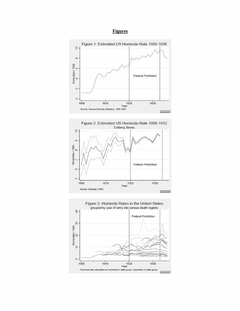
Figure 1 presents the annual raw homicide rate in the United States, based on the
published estimates in the Census Mortality statistics. To the naïve observer, there
appears to be a rapid rise during the early 20th century, with an equally precipitous
decline after 1933. This graph is still presented by the popular media as evidence that
Federal Prohibition was associated with a net increase in the murder rate.11 The increase
between 1900 and 1933, however, has been shown to be almost entirely due to the
sequential addition of states to the registration area, with some additional undercounting
of homicides prior to 1907 [Eckberg (1995)].
In 1995, Douglas Eckberg used back casting to generate an adjusted national
homicide rate (figure 2), which was most notable for the absence of a dramatic “crime
9 Data on suicides are downloaded from Miller, G “State Mortality Data 1900-1936”,http://www.nber.org/data/vital-statistics-deaths-historical/ 10 The list of possible external causes of death in 1907 are: suicide, fracture and dislocations, burns and scalds, heat and sunstroke, cold and freezing, lightening, drowning, inhalation of poisonous gasses, other accidental poisonings, accidental gunshot wounds, injuries by machinery, injuries in mines and quarries, railroad accidents, street car accidents, injuries by vehicles and horses, injuries at birth, and homicide. With the exception of lightening and injuries at birth, all of these causes could plausibly be improperly categorized homicides. Beginning in 1910, homicides and suicides are categorized by method (gun shot, stabbing, hanging, etc.). 11 See, for example, a graph published in Forbes magazine article in 1994, available at http://www.druglibrary.org/schaffer/library/graphs/29.htm, and Moskos (2008) pg. 171.
12
wave.” These adjusted figures are now commonly used to examine early trends in
homicides [Jensen (2000), Donohue and Wolfers (2004)], although Miron (1999) uses
unadjusted numbers. This paper builds on existing research by exploiting both variation
in pre-Federal Prohibition laws, as well as the intensity of temperance laws in each state.
Figure 3 divides states into one of 21 groups, based on when those states entered the
nation death registry. It is clear that neither the murder rate nor the trend in the murder
rate is orthogonal to when a state was entered in the “national” figure, and states entering
just before the passage of Federal Prohibition had particularly high murder rates.
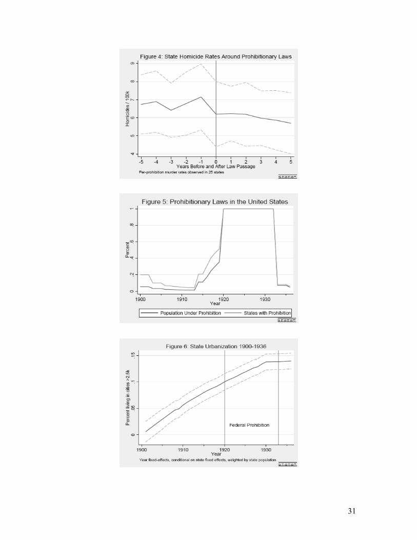
Figures 1-3 sequentially cast doubt on the assertion that Federal Prohibition
necessarily increased the homicide rate. However, these figures ignore the passage of
state temperance laws. In Figure 4, I present the mean state level homicide rates around
the passage of the first temperance law affecting each state. In contrast with the existing
studies, there is a discreet drop in homicide rates after alcohol sales are outlawed. While
the sample underlying this average varies over time, and the standard errors around this
mean estimate are large, Figure 4 is the first evidence that driving the alcohol market
underground may actually be associated with a net reduction in violence.
After a state passes a temperance law, any disputes arising in the continued
purchase or sale of alcohol would have to be resolved through informal and potentially
violent channels. It follows that violent disputes over alcohol would only occur if
individuals continued to attempt to buy alcohol, as opposed to just producing their own
supply or importing small amounts from out of state, a common allowance in local
prohibitionary laws [Merz (1969) pg. 20-23]. It should therefore be the case that violence
due to market informality should be proportional to the frequency with which residents of

13
“dry” states purchased alcohol in violation of state law- the demand for commercial
alcohol.
I take advantage of two sources of data on demand for illegal alcohol. First, in 25
states the question of alcohol prohibition was put to popular vote. The results of these
state votes are published in the appendix of Merz (1969). I use the ratio of votes against
temperance to votes for temperance as a proxy for demand for illegally acquired alcohol
in that state. There was a fair amount of variation in the popularity of the state laws; the
Wet vote was over 90% of the Dry vote in 6 states (Washington, Colorado, Kansas, North
Dakota, Ohio, and Kentucky), but less than 40% of the Dry vote in Maine, Utah,
Wyoming and Idaho. Second, I also construct a similar measure based on the fraction of
votes against ratifying the 18th amendment in the state legislatures, also recorded in the
appendix of Merz (1969). Wets received on average 25.7% of the votes as Drys during
the ratification process, with Wets receiving over 80% of the Dry vote in New York and
Pennsylvania, which were also the states with the largest urban centers in 1920.
Assuming that individual taste for alcohol are positively correlated over time, in states
where there were more Wets relative to Drys, there should have been (weakly) more
alcohol consumption and (weakly) more illegal alcohol sales than in states where there
were few Wets, leading to more homicides due to both systemic and
psychopharmacological effects of alcohol.
In the 19th century whiskey was the most popular alcoholic beverage in America.
Waves of German immigration in the 1840s and 1850s, however, contributed to beer
overtaking whiskey as the most heavily consumed alcoholic beverage in 1890. The fact
that beer, rather than distilled alcohol, was the most popular alcohol beverage has
14
implications for how alcohol regulations in one states could affect the national price of
alcohol. Major distillers were geographically clustered; fourteen plants in Peoria, Illinois
produced approximately 40% of US liquor, and 85% of the hard liquor was produced in
four states [Hamm (1995)]. At the same time, the nature of beer production lead to a
more disperse location pattern; only five states did not produce beer in 1880. In addition,
technological advances in pasteurization, refrigeration and bottling at the end of the 19th
century meant that brewers operated in a national, as opposed to regional, market [Hamm
(1995)]. This implies that the price of beer in any state should be positively correlated
with the number of dry states. Further, the difficulty of obtaining illegal alcohol in a dry
state, and by implication potential profits and the level of violence sustainable in the
underground market, should be increasing in the number of dry states.
A predicted positive relationship between price and violence in temperance states
follows from two observations. First, like, cocaine and heroin, alcohol is an experience
good- consumers do not purchase the pure intoxicant, but a diluted version of uncertain
purity. When the cost of the pure intoxicant increases, the first order effect is for sellers
to dilute the product. The resulting uncertainty about the quality of the product at the
time of sale leads to increased likelihood of violent disputes between customers and
producers over said quality [Reuter and Caulkins (2004)]. Second, increases in the cost
of production will drive some alcohol producers out of business. To the extent that
remaining illegal firms will compete over the new market, there will be a temporary
increase in violence between different sellers until a new equilibrium is established
[Saner et al (1995)]. I therefore expect that in states which have outlawed alcohol
15
markets, increases in the price of illegal alcohol will be associated with an increase in
systemic violence.
IV. Analytic Framework:
Previous research on alcohol temperance and crime have used a time series
approach, examining whether or not murder rates were unusually high during temperance
relative to murder rates before and afterwards, either at the national level [Miron (1999);
Jenson (2000)] or in a specific geographic area [Asbridge and Weerasinghe (2009)].
These time series analyses rely on the assumption that it is possible to construct a
counterfactual murder rate during temperance periods based on the similarly defined
murder rates before and after temperance. For the national data, this is a strong
assumption. Prior to 1933, the number of states included in the national mortality data
increased almost every year. Since the measurement error in the dependant variable (the
national mortality rate) will be correlated with the year of observation by construction,
interpreting the value of a coefficient on what is essentially a dummy for the years 1920
to 1933 is problematic.
Asbridge and Weerasinghe (2009) avoid this issue by using the Chicago Police
Department records, which cover the entire time period. However, they must assume that
no other variable was correlated with homicide rates and the timing of Federal
Prohibition. One obvious confounding variable is the urbanization of the US population.
While the exact mechanism is unclear, urban areas consistently have higher crime rates
than rural areas or small cities [Glaeser and Sacerdote (1999)]. During the early 20th
century, the fraction of US residents living in cities with more than 2,500 residents
16
increased rapidly through 1920, was flat in the 1930 census, and then continued upward
after 1940. The fraction of those urban residents living in “large” cities (more than 250k
residents) also rose dramatically between 1880 and 1920 and began to fall after 1940,
roughly during the same time period that murder rates in the United States turned
downwards as well.
The observed trends in urbanization suggest that multivariate analysis is
necessary to identify the link between illegal markets for alcohol and violence. I examine
the connection between market illegality and violent crime using a standard fixed effects
approach, which takes advantage of state level variation in homicide rates and market
legality. My basic model of the murder rate in state s in year t is as follows
eq 1: ( ) stststtsst emperanceTXMurderLn εβθδα ++++=
where Murderst is the number of homicides per 100k state residents,12 as reported in the
Census Mortality Data. I allow for time invariant differences in the murder rate across
states, as well as arbitrary shocks to the murder rate each year that are common to every
state. I include the values of other variables that may be correlated with both the murder
rate and the timing of temperance laws in the matrix Xst , such as the fraction of the state
that is non-white, the fraction of the state that is foreign born, the log of the state wage,
an estimate of the fraction the population with a elementary school education, as well as
the fraction of the state that lives in a city with more than 2,500 people. All of these
variables, measured in the decennial census, are taken from Haines (2004) with linear
12 I add 0.001 to all homicides to avoid missing observations.
17
interpolations between years. The coefficient of interest is β, my estimate of the
relationship between whether or not state s has prohibited the commercial sale of alcohol
in year t and the corresponding murder rate. Because this variable is equal to one in all
states between 1920 and 1933, my identification is based on the murder rates in the states
which either enacted temperance laws prior to 1920 or kept them on the books after 1933,
and participated in the Census death registry during those years. As is standard in fixed
affects analysis, I allow for arbitrary correlation in the unexplained component of the
murder rate, εst, within each state over time.
While the approach in equation 1 will prevent me from identifying the impact of
market illegality on violence off of measurement error in the national mortality statistics,
as noted above, I am unable to identify the effect of Federal Prohibition per se on violent
crime, since this simultaneously affected alcohol markets in all states. In addition, the
estimated value of β captures the net effect of market illegality on crime- both the
theoretically expected reduction due to lower alcohol consumption and the increase due
to market informality. While it is unclear how to directly separate these two mechanisms,
I can take advantage of the fact that there was likely to be heterogeneity across states in
the size of illegal alcohol market and over time in the price of illegal alcohol.
The quantity of alcohol demanded after temperance is assumed to be positively
correlated with the demand for alcohol prior to the passage of a temperance law.
Assuming that drinkers vote in their best interest, and it is in the best interest of drinkers
for alcohol markets to be legal, one would expect larger illegal markets and thus more
systemic violence in areas where prohibitionary laws were unpopular. Specifically, in
states where there was a high demand for alcohol, one would expect temperance laws to
18
be passed by a smaller margin than in states where the demand for alcohol consumption
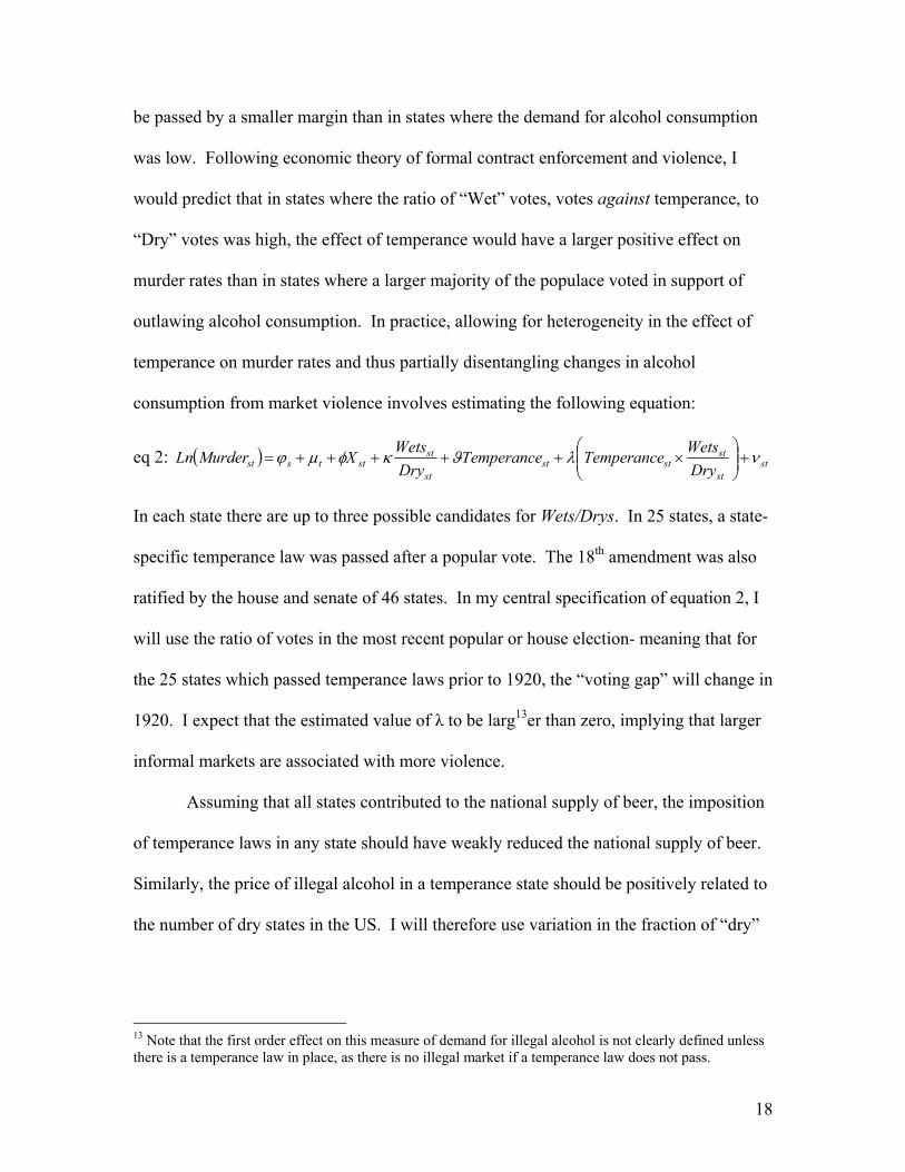
was low. Following economic theory of formal contract enforcement and violence, I
would predict that in states where the ratio of “Wet” votes, votes against temperance, to
“Dry” votes was high, the effect of temperance would have a larger positive effect on
murder rates than in states where a larger majority of the populace voted in support of
outlawing alcohol consumption. In practice, allowing for heterogeneity in the effect of
temperance on murder rates and thus partially disentangling changes in alcohol
consumption from market violence involves estimating the following equation:
eq 2: ( ) stst
ststst
st
ststtsst Dry
WetsemperanceTemperanceTDryWetsXMurderLn νλϑκφμϕ +⎟⎟
⎠
⎞⎜⎜⎝
⎛×+++++=
In each state there are up to three possible candidates for Wets/Drys. In 25 states, a state-
specific temperance law was passed after a popular vote. The 18th amendment was also
ratified by the house and senate of 46 states. In my central specification of equation 2, I
will use the ratio of votes in the most recent popular or house election- meaning that for
the 25 states which passed temperance laws prior to 1920, the “voting gap” will change in
1920. I expect that the estimated value of λ to be larg13er than zero, implying that larger
informal markets are associated with more violence.
Assuming that all states contributed to the national supply of beer, the imposition
of temperance laws in any state should have weakly reduced the national supply of beer.
Similarly, the price of illegal alcohol in a temperance state should be positively related to
the number of dry states in the US. I will therefore use variation in the fraction of “dry”
13 Note that the first order effect on this measure of demand for illegal alcohol is not clearly defined unless there is a temperance law in place, as there is no illegal market if a temperance law does not pass.
19
states in the Census death registry as a proxy for variation in the market price of alcohol.
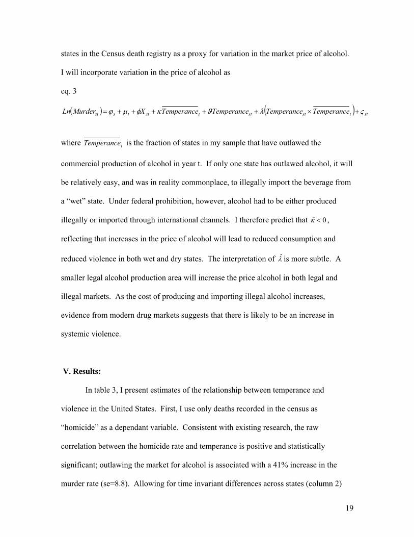
I will incorporate variation in the price of alcohol as
eq. 3
( ) ( ) sttststtsttsst emperanceTemperanceTemperanceTemperanceTXMurderLn ςλϑκφμϕ +×+++++=
where tTemperance is the fraction of states in my sample that have outlawed the
commercial production of alcohol in year t. If only one state has outlawed alcohol, it will
be relatively easy, and was in reality commonplace, to illegally import the beverage from
a “wet” state. Under federal prohibition, however, alcohol had to be either produced
illegally or imported through international channels. I therefore predict that 0ˆ <κ ,
reflecting that increases in the price of alcohol will lead to reduced consumption and
reduced violence in both wet and dry states. The interpretation of λ̂ is more subtle. A
smaller legal alcohol production area will increase the price alcohol in both legal and
illegal markets. As the cost of producing and importing illegal alcohol increases,
evidence from modern drug markets suggests that there is likely to be an increase in
systemic violence.
V. Results:
In table 3, I present estimates of the relationship between temperance and
violence in the United States. First, I use only deaths recorded in the census as
“homicide” as a dependant variable. Consistent with existing research, the raw
correlation between the homicide rate and temperance is positive and statistically
significant; outlawing the market for alcohol is associated with a 41% increase in the
murder rate (se=8.8). Allowing for time invariant differences across states (column 2)
20
increases the variation in murder rates explained by this simple model over ten fold, and
the magnitude of the relationship between temperance and violence is cut in half. For
sake of comparison, a three percentage point increase in urbanization (the average within
state standard), is associated with a 16.5% (se=2.94) increase in the murder rate, which is
not statistically different from the effect of temperance. Conditional on urbanization,
outlawing commercial alcohol sales is associated with a precisely estimated 8% increase
in the murder rate, which is non-trivial. In Column 5 of table 3 I include additional
demographic controls that are likely related to homicide rates over time; as expected,
state education levels are negatively correlated with homicide rates, and states with larger
non-native populations also experience higher rates of homicide. The percentage of the
population between 6 and 20 is negatively correlated with violence, which contradicts
criminology theory on age and crime, but is a common empirical result [Evans and
Owens (2007)]. Including controls for these demographic changes, which only increases
the importance of urbanization, eliminates the statistical importance of temperance in
explaining homicide rates. However, a 6% increase in the murder rate is worth pause,
particularly as the statistical imprecision is sensitive to the time period under analysis.
Eliminating the years 1900-1906, when homicides may have been undercounted,
generates an effect that is the same magnitude, but precisely estimated at the 5% level of
significance.
In the final columns of table 3, I allow for temporal variation that affects all states
at all time. Including year fixed effects explicitly identifies the effect of temperance off
of state laws, as opposed to Federal Prohibition. While Federal Prohibition is associated
with a perhaps substantive (if not statistically) significant effect on murder, when state
21
governments outlawed the sale of alcohol, there was essentially no change in violence-
the estimated effect of temperance is less than one percent, with a standard deviation of
5.4%. The effects of urbanization and demographic changes more broadly, are robust to
the inclusion of state fixed effects.
Is it appropriate to include year fixed effects in this analysis? This is standard
practice when analyzing panel data, but if Federal Prohibition was the key substantive
regulation that outlawed alcohol, state fixed effects may simply not be the right empirical
strategy to take. In the final column of table 3 I impose structure on the relationship
between homicide and time by replacing my year fixed effects with a quadratic time
trend. It is clear that even with restrictive aggregate variation over time, temperance laws
are not correlated with an increase in homicide at the state level. In figure 5 I plot the
number of states which had temperance laws, as well as the fraction of the population
covered by the death registry that lived in a state under temperance. While the variation
in temperance laws is small prior to 1914, up to 30% of the population living in a state
that outlawed alcohol sales prior to 1920. The fact that, conditional on demographic
changes, there was no change in the rate of violence after alcohol was outlawed should
call into question the assertion that legalizing markets reduces violence on net.14
Not all state level temperance laws were equal in their stringency, a point
emphasized by Dills and Miron (2004). In Table 4, I allow for the impact of temperance
laws on murder to vary by whether or not the current law outlawed the possession of
alcohol (prohibition) or allowed the importation or home production of alcohol for
14 In results not presented here, I allow for the impact of Federal Prohibition to be different from state level laws, and alternately eliminate the years 1920-1933 from my sample. I do not find any difference between Federal and state prohibition that cannot be explained by a quadratic time trend, and my results are also robust to excluding Federal Prohibition years.
22
personal use (temperance). Note that all prohibition laws are also temperance laws, but
not all temperance laws are prohibitionary. Without state fixed effects, I cannot identify
the effect of temperance and prohibition separately, but incorporating state fixed effects
(column 2) suggests that all of the positive relationship between murder and temperance
was driven by states which criminalized possession of alcohol as well as commerce- in
those state murder rates increased by 33%, with no change in temperance states.
Interestingly, this effect is robust to controlling for demographic changes (column 4), but
again, not year fixed effects or a quadratic time trend. The statistical precision of this
result is sensitive to the exclusion of the years 1900-1906 (column 5). Setting the results
of columns 5 and 6 temporarily aside, one interpretation of these estimates is that under a
temperance law, individuals with a high or inelastic demand for alcohol can use legal
means to acquire it; either through importation or home distilleries. Only when these
channels are eliminated does a violent illegal market develop. One policy implication is
that a heavily regulated market for illegal substances, with a limited number of suppliers
and a cap on individual consumption might be socially beneficial. This is currently the
approach taken by states with respect to prescription drugs.
The difference between the impact of anti-alcohol laws in prohibition and
temperance states suggests that the residual demand for alcohol was an important
determinant of the violence associated with market illegality. In Table 5 I exploit
variation across states in the demand for alcohol by allowing the impact of prohibition to
be heterogeneous with respect to the potential market for illegal alcohol. As this “market
effect” is continuously defined, I can also identify this effect during Federal Prohibition.
In columns 1 and 2 I test whether or not criminalizing the market for alcohol was
23
associated with increased violence in states where there was likely to be a high residual
demand for alcohol, and find no evidence that this is the case. However, once the
difference in the stringency of temperance laws is taken into account (columns 3 and 4),
an interesting pattern emerges. If a state allows for importation or personal production of
alcohol, there may be as much as a 21% reduction in the murder rate, although this is
only significant at the 90% level of confidence. At the same time, a 10 percentage point
increase in the Wet vote relative to the Dry vote (among temperance states, this is just
under one standard deviation in the voting gap) is associated with a 40% increase in the
homicide rate. However, if the temperance law is outright prohibition, I find no evidence
that murder rates increased in places where prohibition was less popular; specifically, the
sum of the estimated interaction terms in column (3) is 0.012 (se =0.075), and in column
(4) the estimated sum is -0.025, with an estimated standard error of 0.107.
In the final two columns I allow for heterogeneity in the effect of local market
illegality with respect to the overall legality, allowing for a quadratic time trend. Again,
the first order effect of imposing a temperance law (column 5) is a 16% reduction in
murder rates. Consistent with the existence of a national market for alcohol, the fraction
of states restricting the sale of alcohol is also negatively related to violence. However, if
other states impose temperance laws as well, this effect is undone; there is no relationship
between the fraction of states under temperance and homicide in states that already have
temperance laws in place. In column 6, I allow for this effect to vary in prohibition and
temperance states. These “price” effects appear to be driven by states under outright
prohibition, but I am unable to identify any statically significant relationship between
alcohol market legality and violence. Finally, regardless of specification, the relationship
24
between urbanization, education, and immigration is robust. Variation in my measures of
state level demographic change is rudimentary, but even these basic controls explain
variation in homicide far better than availability of legal contract enforcement in the
market for alcohol.
VI. Alternate Measures of Violence
Homicide is a rare event that is only occasionally the outcome of violence. For
example, in 2004 there were roughly 4.3 aggravated assaults for every 1,000 people,
almost 100 times the murder rate of 5.9 per 100k. In addition, the Census Death Registry
likely undercounted homicides prior to 1907 [Eckberg (1995)]. While a systematic
undercounting of homicides should be accounted for by year fixed effects, I now explore
the sensitivity of my results to alternate definitions of homicide; homicides plus suicides
and accidents involving firearms, all deaths involving firearms, all suicides, and all
externally caused or “violent” deaths.15
As shown in Table 6, I find no evidence that conditional on urbanization and
demographic characteristics, violent deaths increased when alcohol markets were
outlawed. At the same time, I consistently estimate that a 1 percentage point increase in
urbanization increases the violent death rate by between 1.5 to 3.4%. Increased
immigration is also associated with firearm related deaths; a one percentage point in
immigration (primarily Southern and Eastern Europeans during this time period) is
associated with a 4 to 6% increase in death by firearm, but only weakly related to violent
deaths in general. As shown in Table 7, I find no evidence of a heterogeneous effect on
15Replicating the results of this paper with for only the years 1907-1936 produces qualitatively similar but less precise results, with the exception of the result noted in the text.
25
violence with respect to the severity of temperance laws (with the exception of a 7%
reduction in externally caused deaths when I do not allow for year fixed effects). Finally,
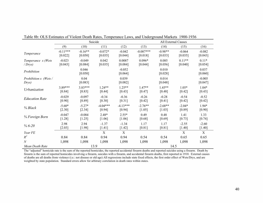
in Tables 8a and 8b I replicate Table 5 for each alternate measure of violence. In no case
do I estimate a net positive effect of temperance on violence. If anything, I consistently
find that suicides fall when alcohol markets are outlawed, which is consistent with
modern research on alcohol consumption and suicide, although the causal relationship
between the two is unclear [Varnik et al (2007)].
VII. Conclusion:
The popular mythology of prohibition involves formerly law abiding adults
become flagrant law breakers; corrupt temperance officials being bribed by bar tenders
and speakeasies being held up by mobsters. Americans demanded alcohol, and
prohibiting the sale of liquor simply drove the market into the hands of organized crime,
increasing the rate of violence in society. This story has both theoretical and anecdotal
appeal; whenever individuals engage in economic transactions, it is inevitable that
disputes between the parties involved will arise. When no formal institution to resolve
those conflicts exists, conflicts are inevitably resolved by “systemic violence.” While no
official crime statistics are available, the available homicide rates in the early 20th century
suggest that homicide spiked during the 1920s and fell after the passage of the 21st
amendment. This pattern of homicides has been regularly used as evidence that current
laws prohibiting the sale of other intoxicating substances have the perverse effect of
increasing violence; part of the reason the “crack epidemic” was so violent was because
crack was illegal.
26
In this paper, I test this theory by exploiting two previously unexamined (but not
unknown) facts about alcohol prohibition; the variation in the timing of state laws
preempting the 18th amendment and superseding its repeal, and the panel nature of the
Census Mortality Statistics. Contrary to conventional wisdom, I find no evidence that, on
net, criminalizing the commercial sale of alcohol increased the murder rate. The apparent
national trend in homicides during prohibition was driven instead by urbanization and the
changing demographic composition of the population. That said, my results support
economic theory of underground markets being associated with violence. When alcohol
markets were criminal (but alcohol consumption per se was not illegal) the political
unpopularity of alcohol temperance was positively related to the homicide rate.
However, even taking this underground into account, the net effect of criminalizing
alcohol was to reduce, not increase, homicides, plausibly through reduced alcohol
consumption. Systemic violence is an important source of harm associated with drug
use. At the same time, systemic violence in the market for alcohol does not appear to
have been a major cause of crime in the 19th century.
27
References:
Abadinsky, Howard (1994) Organized Crime. Fourth edition/ Chicago: Nelson Hall
Incorporated. Asbridge, M. and Weerasinghe, S. (2009) “Homicide in Chicago from 1890 to 1930:
prohibition and it’s impact on alcohol and non-alcohol related homicides” Addiction 104: 355-364.
Blumstein, A. (1995) “Youth Violence, Guns and the Illicit Drug Industry” The Journal
of Criminal Law and Criminology 86(1): 10-36. Boyum, D. and Kleiman, M. (2002) “Substance Abuse Policy from a Crime Control
Perspective” In: J. Q. Wilson and J. Petersilia, [Eds] Crime: Public Policies for Crime Control Oakland: ICS Press. 331-382.
Boyum, D. and Reuter, P. (1996) An Analytic Assessment of US Drug Policy
Washington, DC: American Enterprise Institute Press. Carpenter, C. (2008) “Heavy Alcohol Use and Crime: Evidence from Underage Drunk
Driving Laws.” Journal of Law and Economics 50(3): 539-557. Caulkins, J., Reuter, P. & L. Taylor (2005) “Can Supply Restrictions Lower Price: Illegal
Drugs, Violence and Positional Advantage” Contributions to Economic Analysis and Policy
Cook, P., and Moore, M. (1993) "Violence Reduction through Restrictions on Alcohol
Availability." Alcohol Health & Research World 17(2): 151-156. Dills, A. and Miron, J. (2004) “Alcohol Prohibition and Cirrhosis” American Law and
Economics Review 6(2): 285-317. Dobkin, C. and Carpenter, C. (2008) “The Drinking Age, Alcohol Consumption, and
Crime.” mimeo. Donohue III J. J., Levitt S. D. (1998) “Guns, Violence, and the Efficiency of Illegal
Markets” The American Economic Review 88(2): 463-467. Donohue III J. J., and Wolfers, J. (2004) “Uses and Abuses of Empirical Evidence in the
Death Penalty Debate” Stanford Law Review 58: 791-846. Eckberg, D. (1995) “Estimates of Early Twentieth-Century U/S/ Homicide Rates: an
Econometric Forecasting Approach” Demography 32(1): 1-16. Evans, W. and Owens, E. (2007) “COPS and Crime” Journal of Public Economics
91:181-201.
28
Glaeser, E. and Sacerdote, B. (1999) “Why is There More Crime in Cities?” Journal of Political
Economy 107(6):225-258. Goldstein, P. (1985) “The Drug/Violence Nexus: A Tripartite Concept Framework”
Journal of Drug Issues 14:493-506. Goldstein, P., Brownstein, H. and Ryan, P. (1992) “Drug-Related Homicide in New
York: 1984 and 1988” Crime and Delinquency 38: 459-476. Greenfeld, L. A. (1998) “Alcohol and Crime: An Analysis of National Data on the
Prevalence of Alcohol Involvement in Crime.” National Institute of Justice Research Report # NCJ168632
Haines, Michael R., and the Inter-university Consortium for Political and Social
Research. HISTORICAL, DEMOGRAPHIC, ECONOMIC, AND SOCIAL DATA: THE UNITED STATES, 1790-2000 [Computer file]. ICPSR02896-v2. Hamilton, NY: Colgate University/Ann Arbor: MI: Inter-university Consortium for Political and Social Research [producers], 2004. Ann Arbor, MI: Inter-university Consortium for Political and Social Research [distributor], 2005-04-29. doi:10.3886/ICPSR02896
Hamm, R. (1995) Shaping the Eighteenth Amendment: Temperance Reform,
Legal Culture, and the Polity, 1880–1920. Chapel Hill: University of North Carolina Press.
Jensen, G. (2000) “Prohibition, Alcohol, and Murder: Untangling Countervailing
Mechanisms” Homicide Studies 4(1):18-36. Joksch, H. C., and Jones, R. K. (1993). “Changes in the Drinking Age and Crime.”
Journal of Criminal Justice 21: 209-221. Lewis, M. (2008) “Access to Saloons, Wet Voter Turnout, and Statewide Prohibition
Referenda, 1907–1919” Social Science History 32(3): 373-404. Markowitz, S., and Grossman, M. (2000) “The effects of beer taxes on physical child
abuse.” Journal of Health Economics. 19(2) 271-282. MacCoun, R. and Reuter, P. (1998) “Drug Control” in M. Tonry [Ed.] The Handbook of Crime and Punishment New York: Oxford University Press. 207 – 238. Merz, C. (1969) The Dry Decade. Seattle: University of Washington Press. Miczek, K. A., DeBold, J. F., Haney, M., Tidey, J., Vivian, J. and Weerts, E. (1994)
“Alcohol, Drugs of Abuse, Aggression, and Violence” in A. Reiss, Jr. and J. Roth [Eds.] Understanding and Preventing Violence Volume 3: Social Issues. Washington, DC: National Academy Press. 377-570.
29
Miron, J. (1999) “Violence and the U.S. Prohibition of Drugs and Alcohol” American
Law and Economic Review 1(1/2): 78-114. Moskos, P. (2008) Cop in the Hood: My Year Policing Baltimore’s Eastern District
Princeton: Princeton University Press. Reuter, P. and Caulkins, J. (2004) “Illegal “lemons”: price dispersion in cocaine and
heroin markets” Bulletin on Narcotics 56(1,2):141-165. Reuter, P. (1985) The Organization of Illegal Markets: An Economic Analysis
Washington, DC: National Institute of Justice. Saner, H., MacCoun, R. and Reuter, P. (1995) “On the ubiquity of drug selling among youthful offenders in Washington, DC, 1985-1991: Age, period, or cohort effect?” Journal of Quantitative Criminology 11: 337-362. Schmeckebier, L. (1929) The Bureau of Prohibition: Its History, Activities, and
Organization. Washington: Brooking Institution. Varnik, A. Kolves, K., Vali, Marika, Tooding, L. and Wasserman, D. (2007) “Do alcohol
restrictions reduce suicide mortality?” Addiction 102(2):251-256
Figures
31
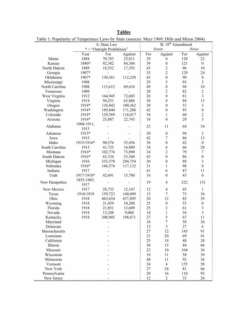
TablesTable 1: Popularity of Temperance Laws by State (sources: Merz 1969; Dills and Miron 2004)
A: State Law * = “Outright Prohibition”
B: 18th Amendment Senate House Year For Against For Against For Against
Maine 1884 70,783 23,811 29 0 120 22 Kansas 1880* 92,302 84,304 39 0 121 0
North Dakota 1889 18,552 17,393 43 2 96 10 Georgia 1907* - - 35 2 129 24
Oklahoma 1907* 130,361 112,258 43 0 90 8 Mississippi 1908 - - 29 5 93 3
North Carolina 1908 113,612 69,416 49 0 94 10 Tennessee 1909 - - 28 2 82 2
West Virginia 1912 164,945 72,603 26 0 81 3 Virginia 1914 94,251 63,886 30 8 84 13 Oregon 1914* 136,842 100,362 30 0 53 3
Washington 1914* 189,840 171,208 42 0 93 0 Colorado 1914* 129,589 118,017 34 1 60 2 Arizona 1914* 25,887 22,743 18 0 29 3
Alabama 1908-1911, 1915 - - 23 11 64 34
Arkansas 1915* - - 30 0 94 2 Iowa 1915 - - 42 7 86 13 Idaho 1915/1916* 90,576 35,456 38 0 62 0
South Carolina 1915 41,735 16,809 34 6 66 28 Montana 1916* 102,776 73,890 34 2 79 7
South Dakota 1916* 65,334 53,360 43 0 86 0 Michigan 1916 353,378 284,754 30 0 88 3 Nebraska 1916* 146,574 117,132 31 1 98 0 Indiana 1917 - - 41 6 87 11
Utah 1917/1918* 42,691 15,780 16 0 43 0
New Hampshire 1855-1903, 1917 - - 19 4 222 131
New Mexico 1917 28,732 12,147 12 4 45 1 Texas 1918/1919 159,723 140,099 15 7 73 36 Ohio 1918 463,654 437,895 20 12 85 29
Wyoming 1918 31,439 10,200 25 0 53 0 Florida 1918 21,851 13,609 25 2 61 3 Nevada 1918 13,248 9,060 14 1 34 3
Kentucky 1918 208,905 198,671 27 5 67 11 Maryland - 18 7 58 36 Delaware - 13 3 27 6
Massachusetts - 27 12 145 91 Louisiana - 21 20 69 41 California - 25 14 48 28
Illinois - 30 15 84 66 Missouri - 22 10 104 36
Wisconsin - 19 11 58 39 Minnesota - 48 11 92 36 Vermont - 24 4 155 58
New York - 27 24 81 66 Pennsylvania - 29 16 110 93 New Jersey - 12 2 33 24
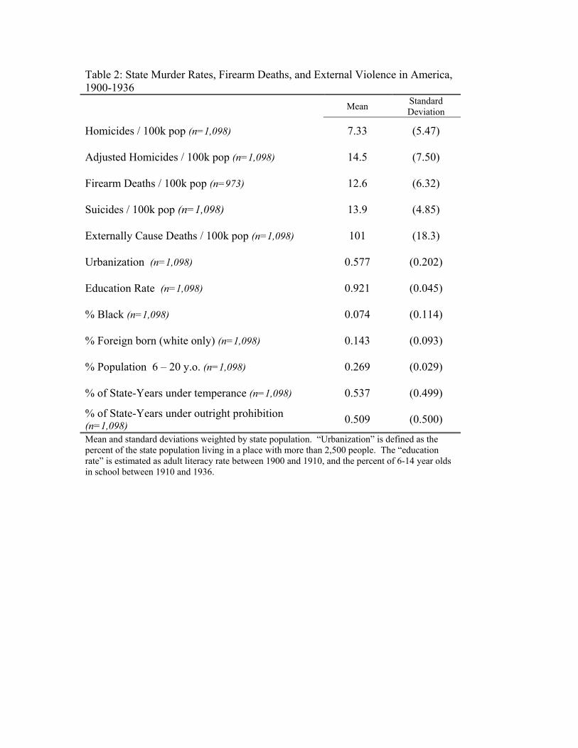
Table 2: State Murder Rates, Firearm Deaths, and External Violence in America, 1900-1936
Mean Standard Deviation
Homicides / 100k pop (n=1,098) 7.33 (5.47)
Adjusted Homicides / 100k pop (n=1,098) 14.5 (7.50)
Firearm Deaths / 100k pop (n=973) 12.6 (6.32)
Suicides / 100k pop (n=1,098) 13.9 (4.85)
Externally Cause Deaths / 100k pop (n=1,098) 101 (18.3)
Urbanization (n=1,098) 0.577 (0.202)
Education Rate (n=1,098) 0.921 (0.045)
% Black (n=1,098) 0.074 (0.114)
% Foreign born (white only) (n=1,098) 0.143 (0.093)
% Population 6 – 20 y.o. (n=1,098) 0.269 (0.029)
% of State-Years under temperance (n=1,098) 0.537 (0.499)
% of State-Years under outright prohibition (n=1,098) 0.509 (0.500)
Mean and standard deviations weighted by state population. “Urbanization” is defined as the percent of the state population living in a place with more than 2,500 people. The “education rate” is estimated as adult literacy rate between 1900 and 1910, and the percent of 6-14 year olds in school between 1910 and 1936.
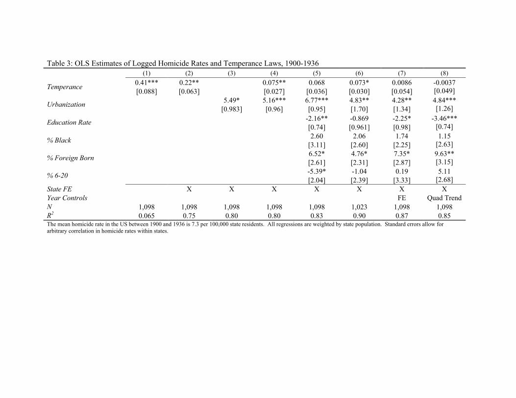
Table 3: OLS Estimates of Logged Homicide Rates and Temperance Laws, 1900-1936 (1) (2) (3) (4) (5) (6) (7) (8)
Temperance 0.41*** 0.22** 0.075** 0.068 0.073* 0.0086 -0.0037 [0.088] [0.063] [0.027] [0.036] [0.030] [0.054] [0.049]
Urbanization 5.49* 5.16*** 6.77*** 4.83** 4.28** 4.84*** [0.983] [0.96] [0.95] [1.70] [1.34] [1.26]
Education Rate -2.16** -0.869 -2.25* -3.46*** [0.74] [0.961] [0.98] [0.74]
% Black 2.60 2.06 1.74 1.15 [3.11] [2.60] [2.25] [2.63]
% Foreign Born 6.52* 4.76* 7.35* 9.63** [2.61] [2.31] [2.87] [3.15]
% 6-20 -5.39* -1.04 0.19 5.11 [2.04] [2.39] [3.33] [2.68]
State FE X X X X X X X Year Controls FE Quad Trend N 1,098 1,098 1,098 1,098 1,098 1,023 1,098 1,098 R2 0.065 0.75 0.80 0.80 0.83 0.90 0.87 0.85 The mean homicide rate in the US between 1900 and 1936 is 7.3 per 100,000 state residents. All regressions are weighted by state population. Standard errors allow for arbitrary correlation in homicide rates within states.
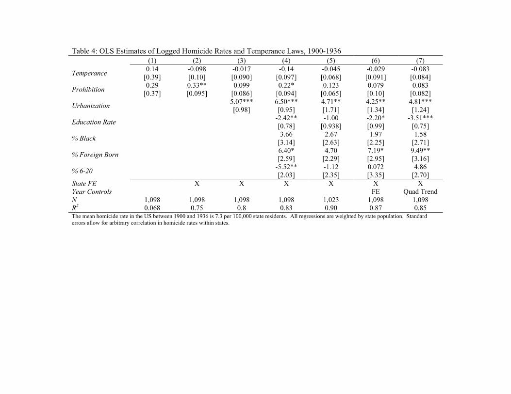
Table 4: OLS Estimates of Logged Homicide Rates and Temperance Laws, 1900-1936 (1) (2) (3) (4) (5) (6) (7)
Temperance 0.14 -0.098 -0.017 -0.14 -0.045 -0.029 -0.083 [0.39] [0.10] [0.090] [0.097] [0.068] [0.091] [0.084]
Prohibition 0.29 0.33** 0.099 0.22* 0.123 0.079 0.083 [0.37] [0.095] [0.086] [0.094] [0.065] [0.10] [0.082]
Urbanization 5.07*** 6.50*** 4.71** 4.25** 4.81*** [0.98] [0.95] [1.71] [1.34] [1.24]
Education Rate -2.42** -1.00 -2.20* -3.51*** [0.78] [0.938] [0.99] [0.75]
% Black 3.66 2.67 1.97 1.58 [3.14] [2.63] [2.25] [2.71]
% Foreign Born 6.40* 4.70 7.19* 9.49** [2.59] [2.29] [2.95] [3.16]
% 6-20 -5.52** -1.12 0.072 4.86 [2.03] [2.35] [3.35] [2.70]
State FE X X X X X X Year Controls FE Quad Trend N 1,098 1,098 1,098 1,098 1,023 1,098 1,098 R2 0.068 0.75 0.8 0.83 0.90 0.87 0.85 The mean homicide rate in the US between 1900 and 1936 is 7.3 per 100,000 state residents. All regressions are weighted by state population. Standard errors allow for arbitrary correlation in homicide rates within states.
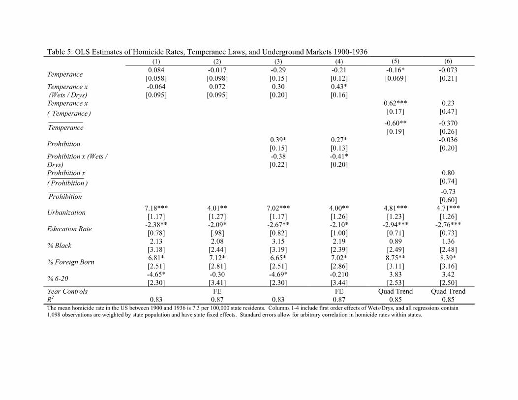
Table 5: OLS Estimates of Homicide Rates, Temperance Laws, and Underground Markets 1900-1936 (1) (2) (3) (4) (5) (6)
Temperance 0.084 -0.017 -0.29 -0.21 -0.16* -0.073 [0.058] [0.098] [0.15] [0.12] [0.069] [0.21]
Temperance x (Wets / Drys)
-0.064 0.072 0.30 0.43* [0.095] [0.095] [0.20] [0.16]
Temperance x ( Temperance )
0.62*** 0.23 [0.17] [0.47]
Temperance -0.60** -0.370 [0.19] [0.26]
Prohibition 0.39* 0.27* -0.036 [0.15] [0.13] [0.20]
Prohibition x (Wets / Drys)
-0.38 -0.41* [0.22] [0.20]
Prohibition x ( ionProhibit )
0.80 [0.74]
ionProhibit -0.73 [0.60]
Urbanization 7.18*** 4.01** 7.02*** 4.00** 4.81*** 4.71*** [1.17] [1.27] [1.17] [1.26] [1.23] [1.26]
Education Rate -2.38** -2.09* -2.67** -2.10* -2.94*** -2.76*** [0.78] [.98] [0.82] [1.00] [0.71] [0.73]
% Black 2.13 2.08 3.15 2.19 0.89 1.36 [3.18] [2.44] [3.19] [2.39] [2.49] [2.48]
% Foreign Born 6.81* 7.12* 6.65* 7.02* 8.75** 8.39* [2.51] [2.81] [2.51] [2.86] [3.11] [3.16]
% 6-20 -4.65* -0.30 -4.69* -0.210 3.83 3.42 [2.30] [3.41] [2.30] [3.44] [2.53] [2.50]
Year Controls FE FE Quad Trend Quad Trend R2 0.83 0.87 0.83 0.87 0.85 0.85 The mean homicide rate in the US between 1900 and 1936 is 7.3 per 100,000 state residents. Columns 1-4 include first order effects of Wets/Drys, and all regressions contain 1,098 observations are weighted by state population and have state fixed effects. Standard errors allow for arbitrary correlation in homicide rates within states.
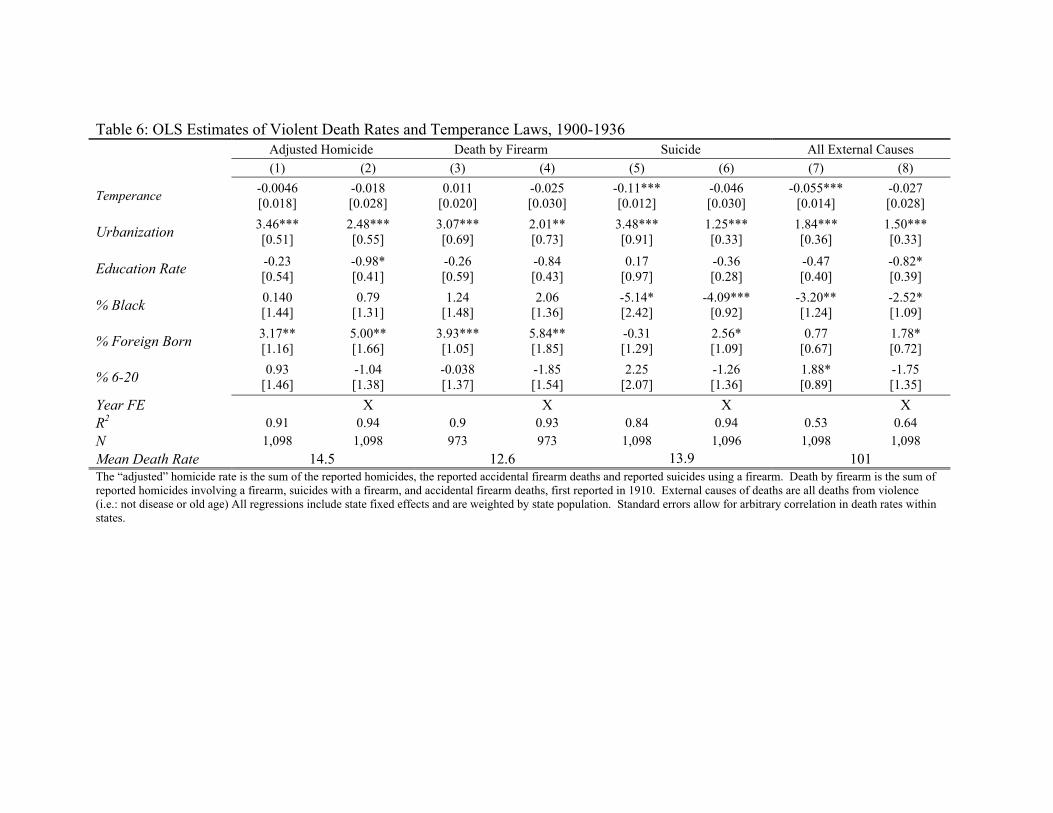
Table 6: OLS Estimates of Violent Death Rates and Temperance Laws, 1900-1936 Adjusted Homicide Death by Firearm Suicide All External Causes (1) (2) (3) (4) (5) (6) (7) (8)
Temperance -0.0046 -0.018 0.011 -0.025 -0.11*** -0.046 -0.055*** -0.027 [0.018] [0.028] [0.020] [0.030] [0.012] [0.030] [0.014] [0.028]
Urbanization 3.46*** 2.48*** 3.07*** 2.01** 3.48*** 1.25*** 1.84*** 1.50*** [0.51] [0.55] [0.69] [0.73] [0.91] [0.33] [0.36] [0.33]
Education Rate -0.23 -0.98* -0.26 -0.84 0.17 -0.36 -0.47 -0.82* [0.54] [0.41] [0.59] [0.43] [0.97] [0.28] [0.40] [0.39]
% Black 0.140 0.79 1.24 2.06 -5.14* -4.09*** -3.20** -2.52* [1.44] [1.31] [1.48] [1.36] [2.42] [0.92] [1.24] [1.09]
% Foreign Born 3.17** 5.00** 3.93*** 5.84** -0.31 2.56* 0.77 1.78* [1.16] [1.66] [1.05] [1.85] [1.29] [1.09] [0.67] [0.72]
% 6-20 0.93 -1.04 -0.038 -1.85 2.25 -1.26 1.88* -1.75 [1.46] [1.38] [1.37] [1.54] [2.07] [1.36] [0.89] [1.35]
Year FE X X X X R2 0.91 0.94 0.9 0.93 0.84 0.94 0.53 0.64 N 1,098 1,098 973 973 1,098 1,096 1,098 1,098 Mean Death Rate 14.5 12.6 13.9 101 The “adjusted” homicide rate is the sum of the reported homicides, the reported accidental firearm deaths and reported suicides using a firearm. Death by firearm is the sum of reported homicides involving a firearm, suicides with a firearm, and accidental firearm deaths, first reported in 1910. External causes of deaths are all deaths from violence (i.e.: not disease or old age) All regressions include state fixed effects and are weighted by state population. Standard errors allow for arbitrary correlation in death rates within states.
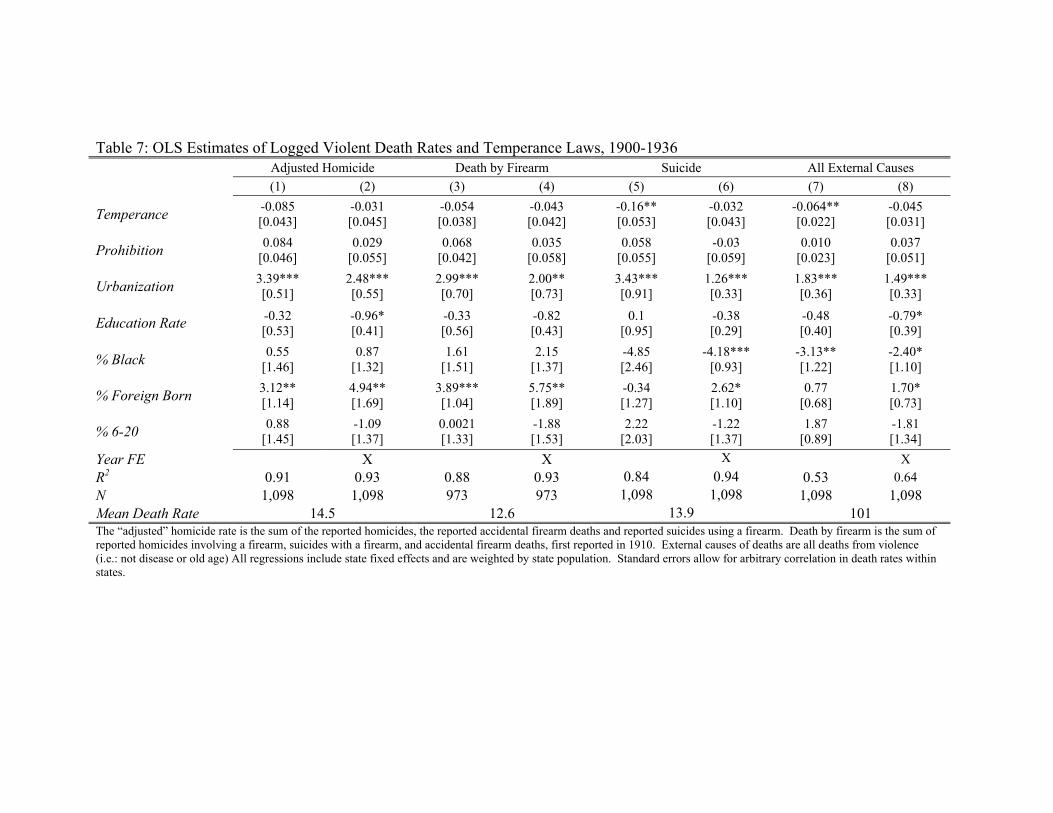
Table 7: OLS Estimates of Logged Violent Death Rates and Temperance Laws, 1900-1936 Adjusted Homicide Death by Firearm Suicide All External Causes (1) (2) (3) (4) (5) (6) (7) (8)
Temperance -0.085 -0.031 -0.054 -0.043 -0.16** -0.032 -0.064** -0.045 [0.043] [0.045] [0.038] [0.042] [0.053] [0.043] [0.022] [0.031]
Prohibition 0.084 0.029 0.068 0.035 0.058 -0.03 0.010 0.037 [0.046] [0.055] [0.042] [0.058] [0.055] [0.059] [0.023] [0.051]
Urbanization 3.39*** 2.48*** 2.99*** 2.00** 3.43*** 1.26*** 1.83*** 1.49*** [0.51] [0.55] [0.70] [0.73] [0.91] [0.33] [0.36] [0.33]
Education Rate -0.32 -0.96* -0.33 -0.82 0.1 -0.38 -0.48 -0.79* [0.53] [0.41] [0.56] [0.43] [0.95] [0.29] [0.40] [0.39]
% Black 0.55 0.87 1.61 2.15 -4.85 -4.18*** -3.13** -2.40* [1.46] [1.32] [1.51] [1.37] [2.46] [0.93] [1.22] [1.10]
% Foreign Born 3.12** 4.94** 3.89*** 5.75** -0.34 2.62* 0.77 1.70* [1.14] [1.69] [1.04] [1.89] [1.27] [1.10] [0.68] [0.73]
% 6-20 0.88 -1.09 0.0021 -1.88 2.22 -1.22 1.87 -1.81 [1.45] [1.37] [1.33] [1.53] [2.03] [1.37] [0.89] [1.34]
Year FE X X X X R2 0.91 0.93 0.88 0.93 0.84 0.94 0.53 0.64 N 1,098 1,098 973 973 1,098 1,098 1,098 1,098 Mean Death Rate 14.5 12.6 13.9 101 The “adjusted” homicide rate is the sum of the reported homicides, the reported accidental firearm deaths and reported suicides using a firearm. Death by firearm is the sum of reported homicides involving a firearm, suicides with a firearm, and accidental firearm deaths, first reported in 1910. External causes of deaths are all deaths from violence (i.e.: not disease or old age) All regressions include state fixed effects and are weighted by state population. Standard errors allow for arbitrary correlation in death rates within states.
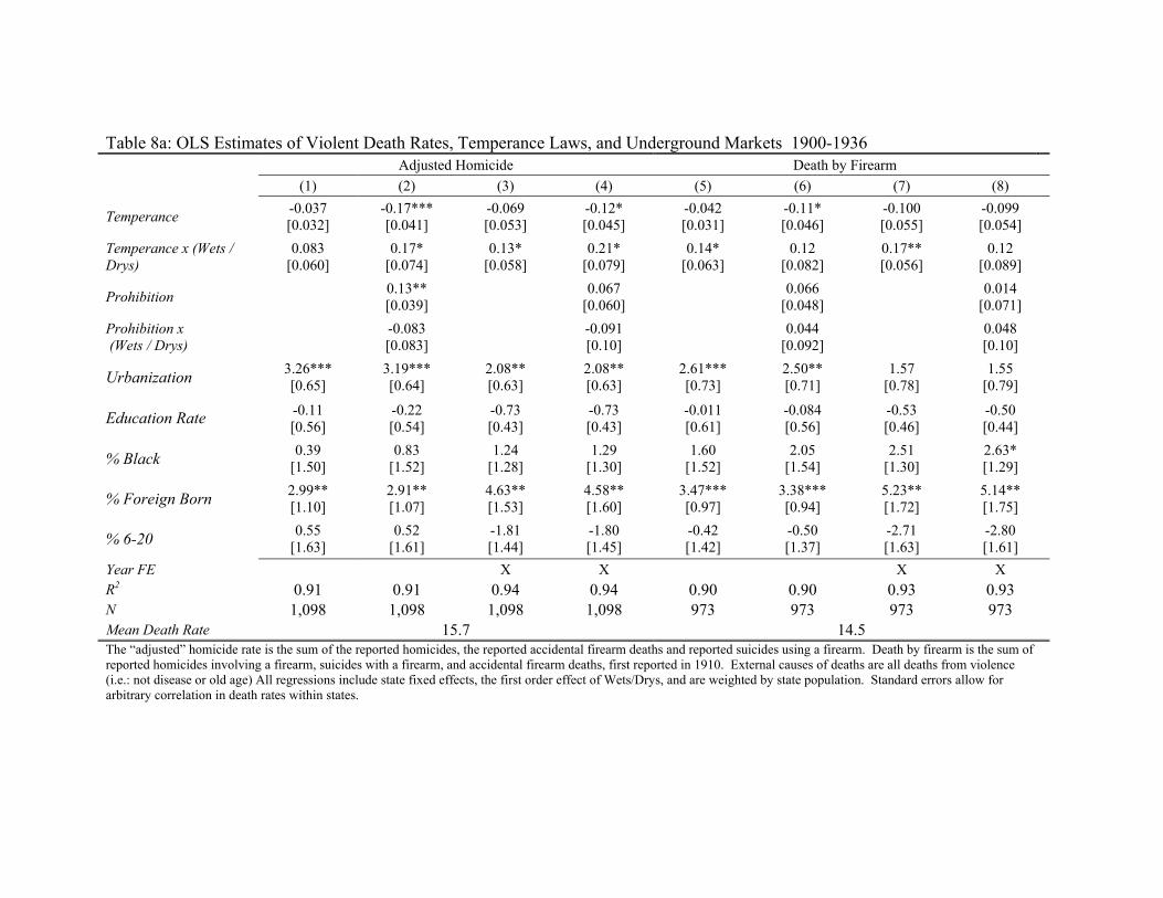
Table 8a: OLS Estimates of Violent Death Rates, Temperance Laws, and Underground Markets 1900-1936 Adjusted Homicide Death by Firearm (1) (2) (3) (4) (5) (6) (7) (8)
Temperance -0.037 -0.17*** -0.069 -0.12* -0.042 -0.11* -0.100 -0.099 [0.032] [0.041] [0.053] [0.045] [0.031] [0.046] [0.055] [0.054]
Temperance x (Wets / Drys)
0.083 0.17* 0.13* 0.21* 0.14* 0.12 0.17** 0.12 [0.060] [0.074] [0.058] [0.079] [0.063] [0.082] [0.056] [0.089]
Prohibition 0.13** 0.067 0.066 0.014 [0.039] [0.060] [0.048] [0.071]
Prohibition x (Wets / Drys)
-0.083 -0.091 0.044 0.048 [0.083] [0.10] [0.092] [0.10]
Urbanization 3.26*** 3.19*** 2.08** 2.08** 2.61*** 2.50** 1.57 1.55 [0.65] [0.64] [0.63] [0.63] [0.73] [0.71] [0.78] [0.79]
Education Rate -0.11 -0.22 -0.73 -0.73 -0.011 -0.084 -0.53 -0.50 [0.56] [0.54] [0.43] [0.43] [0.61] [0.56] [0.46] [0.44]
% Black 0.39 0.83 1.24 1.29 1.60 2.05 2.51 2.63* [1.50] [1.52] [1.28] [1.30] [1.52] [1.54] [1.30] [1.29]
% Foreign Born 2.99** 2.91** 4.63** 4.58** 3.47*** 3.38*** 5.23** 5.14** [1.10] [1.07] [1.53] [1.60] [0.97] [0.94] [1.72] [1.75]
% 6-20 0.55 0.52 -1.81 -1.80 -0.42 -0.50 -2.71 -2.80 [1.63] [1.61] [1.44] [1.45] [1.42] [1.37] [1.63] [1.61]
Year FE X X X X R2 0.91 0.91 0.94 0.94 0.90 0.90 0.93 0.93 N 1,098 1,098 1,098 1,098 973 973 973 973 Mean Death Rate 15.7 14.5 The “adjusted” homicide rate is the sum of the reported homicides, the reported accidental firearm deaths and reported suicides using a firearm. Death by firearm is the sum of reported homicides involving a firearm, suicides with a firearm, and accidental firearm deaths, first reported in 1910. External causes of deaths are all deaths from violence (i.e.: not disease or old age) All regressions include state fixed effects, the first order effect of Wets/Drys, and are weighted by state population. Standard errors allow for arbitrary correlation in death rates within states.
40
Table 8b: OLS Estimates of Violent Death Rates, Temperance Laws, and Underground Markets 1900-1936 Suicide All External Causes (9) (10) (11) (12) (13) (14) (15) (16)
Temperance -0.11*** -0.16** -0.072* -0.042 -0.087*** -0.98** -0.064 -0.082 [0.022] [0.050] [0.035] [0.044] [0.018] [0.033] [0.035] [0.043]
Temperance x (Wets / Drys)
-0.023 -0.049 0.042 0.0087 0.096* 0.085 0.11** 0.11* [0.043] [0.084] [0.035] [0.084] [0.044] [0.056] [0.040] [0.054]
Prohibition 0.046 -0.052 0.010 0.037 [0.050] [0.064] [0.028] [0.060]
Prohibition x (Wets / Drys)
0.04 0.039 0.014 -0.005 [0.083] [0.082] [0.048] [0.047]
Urbanization 3.89*** 3.83*** 1.24** 1.25** 1.47** 1.45** 1.05* 1.04* [0.84] [0.83] [0.44] [0.43] [0.47] [0.48] [0.42] [0.43]
Education Rate -0.029 -0.097 -0.34 -0.36 -0.26 -0.28 -0.54 -0.52 [0.90] [0.89] [0.30] [0.31] [0.42] [0.41] [0.42] [0.42]
% Black -5.60* -5.27* -4.04*** -4.13*** -2.76** -2.68** -2.04* 1.94* [2.30] [2.34] [0.94] [0.94] [1.05] [1.03] [0.89] [0.90]
% Foreign Born -0.047 -0.084 2.48* 2.55* 0.49 0.48 1.41 1.33 [1.28] [1.25] [1.06] [1.06] [0.68] [0.69] [0.73] [0.74]
% 6-20 2.98 2.94 -1.37 -1.34 1.17 1.17 -2.55 -2.60 [2.03] [1.98] [1.41] [1.42] [0.81] [0.81] [1.40] [1.40]
Year FE X X X X R2 0.84 0.84 0.94 0.94 0.54 0.54 0.65 0.65 N 1,098 1,098 1,098 1,098 1,098 1,098 1,098 1,098 Mean Death Rate 13.9 14.5 The “adjusted” homicide rate is the sum of the reported homicides, the reported accidental firearm deaths and reported suicides using a firearm. Death by firearm is the sum of reported homicides involving a firearm, suicides with a firearm, and accidental firearm deaths, first reported in 1910. External causes of deaths are all deaths from violence (i.e.: not disease or old age) All regressions include state fixed effects, the first order effect of Wets/Drys, and are weighted by state population. Standard errors allow for arbitrary correlation in death rates within states.