Are Sticky Prices Costly? Evidence FromThe Stock Market∗

Yuriy Gorodnichenko† and Michael Weber‡

This version: July 2013

Abstract

We show that after monetary policy announcements, the conditional volatilityof stock market returns rises more for firms with stickier prices than for firmswith more flexible prices. This differential reaction is economically large aswell as strikingly robust to a broad array of checks. These results suggest thatmenu costs—broadly defined to include physical costs of price adjustment,informational frictions, etc.—are an important factor for nominal price rigidity.We also show that our empirical results are qualitatively and, under plausiblecalibrations, quantitatively consistent with New Keynesian macroeconomicmodels where firms have heterogeneous price stickiness. Since our frameworkis valid for a wide variety of theoretical models and frictions preventing firmsfrom price adjustment, we provide “model-free” evidence that sticky prices areindeed costly.

JEL classification: E12, E31, E44, G12, G14

Keywords: menu costs, sticky prices, asset prices, high frequencyidentification∗This research was conducted with restricted access to the Bureau of Labor Statistics (BLS)

data. The views expressed here are those of the authors and do not necessarily reflect the views ofthe BLS. We thank our project coordinator at the BLS, Ryan Ogden, for help with the data and EmiNakamura and Jon Steinsson for making their data available to us. We thank Francesco D’Acunto,Luca Fornaro (discussant), Nicolae Garleanu, Simon Gilchrist, Robert Hall, Nir Jaimovich, HannoLustig, Martin Lettau, Matteo Maggiori, Guido Menzio, Adair Morse, Marcus Opp, FranciscoPalomino (discussant), Raphael Schoenle, Eric Sims, Joe Vavra, seminar participants at UC SantaCruz, the 4th Boston University/ Boston Fed Conference on Macro-Finance Linkages, the ESNASmeeting, the Barcelona Summer Forum, the NBER SI EFG Price Dynamics working group andespecially Olivier Coibion and David Romer for valuable comments. We gratefully acknowledgefinancial support from the Coleman Fung Risk Management Research Center at UC Berkeley.Gorodnichenko also thanks the NSF and the Sloan Research Fellowship for financial support. Weberalso thanks the Minder Cheng Fellowship and the UC Berkeley Institute for Business and EconomicResearch for financial support.†Department of Economics, University of California at Berkeley, Berkeley, USA. email:

ygorodni@econ.berkeley.edu‡Haas School of Business, University of California at Berkeley, Berkeley, USA. email:

michael weber@haas.berkeley.edu.

I Introduction

In principle, fixed costs of changing prices can be observed and measured. In practice,

such costs take disparate forms in different firms, and we have no data on their magnitude.

So the theory can be tested at best indirectly, at worst not at all. Alan Blinder (1991)

Are sticky prices costly? This simple question stirs an unusually heated debate in

macroeconomics. While there seems to be a growing consensus that prices at the

micro-level are fixed in the short run,1 it is still unclear why firms have rigid prices.

A central tenet of New Keynesian macroeconomics is that firms face fixed “menu” costs

of nominal price adjustment which can rationalize why firms may forgo an increase in

profits by keeping existing prices unchanged after real or nominal shocks. However, the

observed price rigidity does not necessarily entail that nominal shocks have real effects

or that the inability of firms to adjust prices burdens firms. For example, Head et al.

(2012) present a theoretical model where sticky prices arise endogenously even if firms

are free to change prices at any time without any cost. This alternative theory has vastly

different implications for business cycles and policy. How can one distinguish between

these opposing motives for price stickiness? The key insight of this paper is that in

New Keynesian models, sticky prices are costly to firms, whereas in other models they

are not. While the sources and types of “menu” costs are likely to vary tremendously

across firms thus making the construction of an integral measure of the cost of sticky

prices extremely challenging, looking at market valuations of firms can provide a natural

metric to determine whether price stickiness is indeed costly. In this paper, we exploit

stock market information to explore these costs and— to the extent that firms equalize

costs and benefits of nominal price adjustment—quantify “menu” costs. The evidence we

document is consistent with the New Keynesian interpretation of price stickiness.

Specifically, we merge confidential micro-level data underlying the producer price

index (PPI) from the Bureau of Labor Statistics (BLS) with stock price data for individual

firms from NYSE Trade and Quote (taq) and study how stock returns of firms with

different frequencies of price adjustment respond to monetary shocks (identified as changes

in futures on the fed funds rates, the main policy instrument of the Fed) in narrow time

windows around press releases of the Federal Open Market Committee (FOMC). To guide

1Bils and Klenow (2004), Nakamura and Steinsson (2008).

2

our empirical analyses, we show in a basic New Keynesian model that firms with stickier

prices should experience a greater increase in the volatility of returns than firms with

more flexible prices after a nominal shock. Intuitively, firms with larger costs of price

adjustment tolerate larger departures from the optimal reset price. Thus, the range in

which the discounted present value of cash flows can fluctuate is wider. The menu cost

in this theoretical exercise is generic and, hence, our framework covers a broad range of

models with inflexible prices.

Consistent with this logic, we find that returns for firms with stickier prices exhibit

greater volatility after monetary shocks than returns of firms with more flexible prices,

with the magnitudes being broadly in line with the estimates one can obtain from a

calibrated New Keynesian model with heterogeneous firms: a hypothetical monetary

policy surprise of 25 basis points (bps) leads to an increase in squared returns of 8%2 for the

firms with stickiest prices. This sensitivity is reduced by a factor of three for firms with the

most flexible prices in our sample. Our results are robust to a large battery of specification

checks, subsample analyses, placebo tests, and alternative estimation methods.2

Our work contributes to a large literature aimed at quantifying the costs of price

adjustment. Zbaracki et al. (2004) and others measure menu costs directly by keeping

records of costs associated with every stage of price adjustments at the firm level (data

collection, information processing, meetings, physical costs). Anderson et al. (2012)

have access to wholesale costs and retail price changes of a large retailer. Exploiting

the uniform pricing rule employed by this retailer for identification, they show that the

absence of menu costs would lead to 18% more price changes. This approach sheds

light on the process of adjusting prices, but it is difficult to generalize these findings

given the heterogeneity of adjustment costs across firms and industries. Our approach

is readily applicable to any firm with publicly traded equity, independent of industry,

country or location. A second strand (e.g., Blinder (1991)) elicits information about costs

and mechanisms of price adjustment from survey responses of managers. This approach

is remarkably useful in documenting reasons for rigid prices but, given the qualitative

nature of survey answers, it cannot provide a magnitude of the costs associated with

2Uncertainty shocks proxied by stock market volatility have recently gained attention as a potentialdriver of business cycles (see among others Bloom (2009)). Our results suggest that one should becautious with using stock market volatility as a measure of uncertainty shocks because conditionalheteroskedasticity could be an outcome of an interaction between differential menu costs and nominal orreal shocks.

3

price adjustment. In contrast, our approach can provide a quantitative estimate of these

costs. A third group of papers (e.g. Klenow and Willis (2007), Nakamura and Steinsson

(2008)) integrates menu costs into fully fledged dynamic stochastic general equilibrium

(DSGE) models. Menu costs are estimated or calibrated at values that match moments

of aggregate (e.g. persistence of inflation) or micro-level (e.g. frequency of price changes)

data. This approach is obviously most informative if the underlying model is correctly

specified. Given the striking variety of macroeconomic models in the literature and limited

ability to discriminate between models with available data, one may be concerned that

the detailed structure of a given DSGE model can produce estimates that are sensitive to

auxiliary assumptions necessary to make the model tractable or computable. In contrast,

our approach does not have to specify a macroeconomic model and thus our estimates are

robust to alternative assumptions about the structure of the economy.3

Our paper is also related to the literature investigating the effect of monetary shocks

on asset prices. In a seminal study, Cook and Hahn (1989) use an event study framework

to examine the effects of changes in the federal funds rate on bond rates using a daily

event window. They show that changes in the federal funds target rate are associated

with changes in interest rates in the same direction with larger effects at the short end of

the yield curve. Bernanke and Kuttner (2005)—also using a daily event window—focus

on unexpected changes in the federal funds target rate. They find that an unexpected

interest rate cut of 25 basis points leads to an increase in the CRSP value weighted

market index of about 1 percentage point. Gurkaynak et al. (2005) focus on intraday

event windows and find effects of similar magnitudes for the S&P500. Weber (2013)

uses non-parametric portfolio sorts and panel regressions to show that sticky price firms

command a cross sectional return premium of up to 4% compared to flexible price firms. In

addition, besides the impact on the level of returns, monetary policy surprises also lead to

greater stock market volatility. For example, consistent with theoretical models predicting

increased trading and volatility after important news announcements (e.g. Harris and

Raviv (1993) and Varian (1989)), Bomfim (2003) finds that the conditional volatility

of the S&P500 spikes after unexpected FOMC policy movements. Given that monetary

3Other recent contributions to this literature are Goldberg and Hellerstein (2011), Eichenbaum et al.(2011) Midrigan (2011), Eichenbaum et al. (2012), Bhattarai and Schoenle (2012), Vavra (2013), Bergerand Vavra (2013). See Klenow and Malin (2010) and Nakamura and Steinsson (2013) for recent reviewsof this literature.

4

policy announcements also appear to move many macroeconomic variables (see e.g. Faust

et al. (2004b)), these shocks are, thus, a powerful source of variation in the data.

There are several limitations to our approach. First, we require information on

returns with frequent trades to ensure that returns can be precisely calculated in narrow

event windows. This constraint excludes illiquid stocks with infrequent trading. We focus

on the constituents of the S&P500 which are all major US companies with high stock

market capitalization.4 Second, our methodology relies on unanticipated, presumably

exogenous shocks that influence the stock market valuation of firms. A simple metric of

this influence could be whether a given shock moves the aggregate stock market. While

this may appear an innocuous constraint, most macroeconomic announcements other

than the Fed’s (e.g. the surprise component of announcements of GDP or unemployment

figures by the Bureau of Economic Analysis (BEA) and BLS) fail to consistently move the

stock market in the U.S. Third, our approach is built on “event” analysis and therefore

excludes shocks that hit the economy continuously. Finally, we rely on the efficiency of

financial markets.5

The rest of the paper is structured as follows. The next section describes how

our measure of price stickiness at the firm level is constructed. Section III lays out a

static version of a New Keynesian model with sticky prices and provides guidance for

our empirical specification. This section also discusses our high frequency identification

strategy employing nominal shocks from fed funds futures and the construction of our

variables and controls. Section IV presents the estimates of the sensitivity of squared

returns to nominal shocks as a function of price stickiness. Section V calibrates a

4The intraday event window restricts our universe of companies to large firms as small stocksin the early part of our sample often experienced no trading activity for several hours even aroundmacroeconomic news announcements contrary to the constituents of the S&P500. Given the high volumeof trades for the latter firms, news are quickly incorporated into stock prices. For example, Zebedee et al.(2008) among others show that the effect of monetary policy surprises is impounded into prices of theS&P500 within minutes.

5Even though the information set required by stock market participants may appear large (frequenciesof price adjustments, relative prices etc.), we document in Subsection E. of Section IV that the effectsfor conditional stock return volatility also hold for firm profits. Therefore, sophisticated investorscan reasonably identify firms with increased volatility after monetary policy shocks and trade on thisinformation using option strategies such as straddles. A straddle consists of simultaneously buying a calland a put option on the same stock with the same strike price and time to maturity and profits fromincreases in volatility. It is an interesting question to analyze the identity of traders around macroeconomicnews announcements: private investors or rational arbitrageurs and institutional investors. Results ofErenburg et al. (2006) and Green (2004) and the fact that news are incorporated into prices within minutesindicate the important role of sophisticated traders around macroeconomic news announcements.

5

dynamic version of a New Keynesian model to test whether our empirical estimates can

be rationalized by a reasonably calibrated model. Section VI concludes and discusses

further applications of our novel methodology.

II Measuring Price Stickiness

A key ingredient of our analysis is a measure of price stickiness at the firm level. We

use the confidential microdata underlying the PPI of the BLS to calculate the frequency

of price adjustment for each firm in our sample. The PPI measures changes in selling

prices from the perspective of producers, as compared to the Consumer Price Index (CPI)

which looks at price changes from the consumers’ perspective. The PPI tracks prices of

all goods producing industries such as mining, manufacturing, gas and electricity, as well

as the service sector. The PPI covers about three quarters of the service sector output.

The BLS applies a three stage procedure to determine the individual goods included in

the PPI. In the first step, the BLS compiles a list of all firms filing with the Unemployment

Insurance system. This information is then supplemented with additional publicly

available data which is of particular importance for the service sector to refine the universe

of establishments.

In the second step, individual establishments within the same industry are combined

into clusters. This step ensures that prices are collected at the price forming unit as several

establishments owned by the same company might constitute a profit maximizing center.

Price forming units are selected for the sample based on the total value of shipments or

the number of employees.

After an establishment is chosen and agrees to participate, a probability sampling

technique called disaggregation is applied. In this final step, the individual goods and

services to be included in the PPI are selected. BLS field economists combine individual

items and services of a price forming unit into categories, and assign sampling probabilities

proportional to the value of shipments. These categories are then further broken down

based on price determining characteristics until unique items are identified. If identical

goods are sold at different prices due to e.g. size and units of shipments, freight type,

type of buyer or color then these characteristics are also selected based on probabilistic

sampling.

The BLS collects prices from about 25,000 establishments for approximately 100,000

6

individual items on a monthly basis. The BLS defines PPI prices as “net revenue accruing

to a specified producing establishment from a specified kind of buyer for a specified

product shipped under specified transaction terms on a specified day of the month”.6

Taxes and fees collected on behalf of federal, state or local governments are not included.

Discounts, promotions or other forms of rebates and allowances are reflected in PPI prices

insofar as they reduce the revenues received by the producer. The same item is priced

month after month. The BLS undertakes great efforts to adjust for quality changes and

product substitutions so that only true price changes are measured.

Prices are collected via a survey which is emailed or faxed to participating

establishments.7 The survey asks whether the price has changed compared to the previous

month and if yes, the new price is asked.8 Individual establishments remain in the sample

for an average of seven years until a new sample is selected in the industry. This resampling

occurs to account for changes in the industry structure and changing product market

conditions within the industry.9

We calculate the frequency of price adjustment as the mean fraction of months with

price changes during the sample period of an item. For example, if an observed price

path is $4 for two months and then $5 for another three months, there is one price change

during five months and hence the frequency is 1/5.10 When calculating the frequency of

price adjustment, we exclude price changes due to sales. We identify sales using the filter

employed by Nakamura and Steinsson (2008). Including sales does not affect our results

in any material way because, as documented in Nakamura and Steinsson (2008), sales are

rare in producer prices.

We aggregate frequencies of price adjustments at the establishment level and further

6See Chapter 14, BLS Handbook of Methods, available under http://www.bls.gov/opub/hom/.7The online appendix contains a sample survey.8This two stage procedure might lead to a downward bias in the frequency of price adjustment.

Using the anthrax scare of 2001 as a natural experiment, Nakamura and Steinsson (2008) show, however,that the behavior of prices is insensitive to the collection method: during October and November 2001all government mail was redirected and the BLS was forced to collect price information via phone calls.Controlling for inflation and seasonality in prices, they do not find a significant difference in the frequencyof price adjustment across the two collection methods.

9Goldberg and Hellerstein (2011) show that forced product substitutions and sales are negligible inthe microdata underlying the PPI.

10We do not consider the first observation as a price change and do not account for left censoring ofprice spells. Bhattarai and Schoenle (2012) verify that explicitly accounting for censoring does not changethe resulting distribution of probabilities of price adjustments. Our baseline measure treats missing pricevalues as interrupting price spells. The appendix contains results for alternative measures of the frequencyof price adjustment; results are quantitatively and statistically very similar.

7

aggregate the resulting frequencies at the company level. The first aggregation is

performed via internal establishment identifiers of the BLS. To perform the firm level

aggregation, we manually check whether establishments with the same or similar names

are part of the same company. In addition, we search for names of subsidiaries and name

changes e.g. due to mergers, acquisitions or restructurings occurring during our sample

period for all firms in our financial dataset.

We discuss the fictitious case of a company Milkwell Inc. to illustrate aggregation to

the firm level. Assume we observe product prices of items for the establishments Milkwell

Advanced Circuit, Milkwell Aerospace, Milkwell Automation and Control, Milkwell Mint,

and Generali Enel. In the first step, we calculate the frequency of product price adjustment

at the item level and aggregate this measure at the establishment level for all of the above

mentioned establishments.11 We calculate both equally weighted frequencies (baseline)

and frequencies weighted by values of shipments associated with items/establishments

(see appendix) say for establishment Milkwell Aerospace. We then use publicly available

information to check whether the individual establishments are part of the same company.

Assume that we find that all of the above mentioned establishments with Milkwell in

the establishment name but Milkwell Mint are part of Milkwell Inc. Looking at the

company structure, we also find that Milkwell has several subsidiaries, Honeymoon, Pears

and Generali Enel. Using this information, we then aggregate the establishment level

frequencies of Milkwell Advanced Circuit, Milkwell Aerospace, Milkwell Automation and

Control and Generali Enel at the company level, again calculating equally weighted and

value of shipments weighted frequencies. Our measure of price stickiness is constant at

the firm level. Allowing for time series variation has little impact on our findings as there

is little time variation in the frequency of price adjustment at the firm level.

Table 1 reports mean probabilities, standard deviations and the number of firm-event

observations for our measures of the frequency of price adjustment, both for the total

sample and for each industry separately.12 The overall mean frequency of price adjustment

(FPA) is 14.66%/month implying an average duration, −1/ln(1−FPA), of 6.03 months.

There is a substantial amount of heterogeneity in the frequency across sectors, ranging

11Items in our dataset are alpha-numeric codes in a SAS dataset and we cannot identify their specificnature.

12The coarse definition of industries is due to confidentiality reasons and also partially explains thesubstantial variation of our measures of price stickiness within industry.

8

from as low as 8.07%/month for the service sector (implying a duration of almost one

year) to 25.35%/month for agriculture (implying a duration of 3.42 months). Finally, the

high standard deviations highlight dramatic heterogeneity in measured price stickiness

across firms even within industries. Different degrees of price stickiness of similar firms

operating in the same industry can arise due to a different customer and supplier structure,

heterogeneous organizational structure or varying operational efficiencies and management

philosophies.13

III Framework

In this section, we outline the basic intuition for how returns and price stickiness are

related in the context of a New Keynesian macroeconomic model. We will focus on one

shock—monetary policy surprises—which has a number of desirable properties.14 While

restricting the universe of shocks to only monetary policy shocks limits our analysis in

terms of providing an integral measure of costs of sticky prices, it is likely to greatly

improve identification and generate a better understanding of how sticky prices and stock

returns are linked. This section also guides us in choosing regression specifications for the

empirical part of the paper and describes how variables are constructed.

A. Static model

We start with a simple, static model to highlight intuition for our subsequent

theoretical and empirical analyses. Suppose that a second-order approximation to a firm’s

profit function is valid so that the payoff of firm i can be expressed as πi ≡ π(Pi, P∗) =

πmax − ψ(Pi − P ∗)2 where P ∗ is the optimal price given economic conditions, Pi is the

current price of firm i, πmax is the maximum profit a firm can achieve and ψ captures

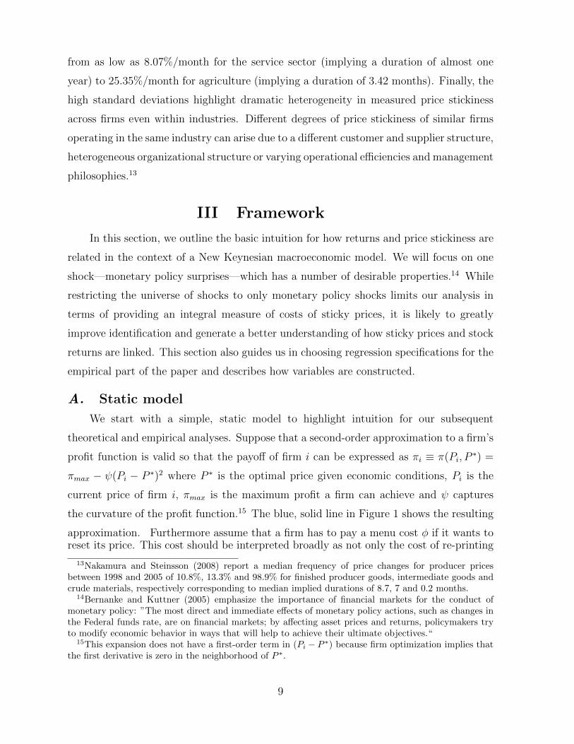
the curvature of the profit function.15 The blue, solid line in Figure 1 shows the resulting

approximation. Furthermore assume that a firm has to pay a menu cost φ if it wants toreset its price. This cost should be interpreted broadly as not only the cost of re-printing

13Nakamura and Steinsson (2008) report a median frequency of price changes for producer pricesbetween 1998 and 2005 of 10.8%, 13.3% and 98.9% for finished producer goods, intermediate goods andcrude materials, respectively corresponding to median implied durations of 8.7, 7 and 0.2 months.

14Bernanke and Kuttner (2005) emphasize the importance of financial markets for the conduct ofmonetary policy: ”The most direct and immediate effects of monetary policy actions, such as changes inthe Federal funds rate, are on financial markets; by affecting asset prices and returns, policymakers tryto modify economic behavior in ways that will help to achieve their ultimate objectives.“

15This expansion does not have a first-order term in (Pi − P ∗) because firm optimization implies thatthe first derivative is zero in the neighborhood of P ∗.

9

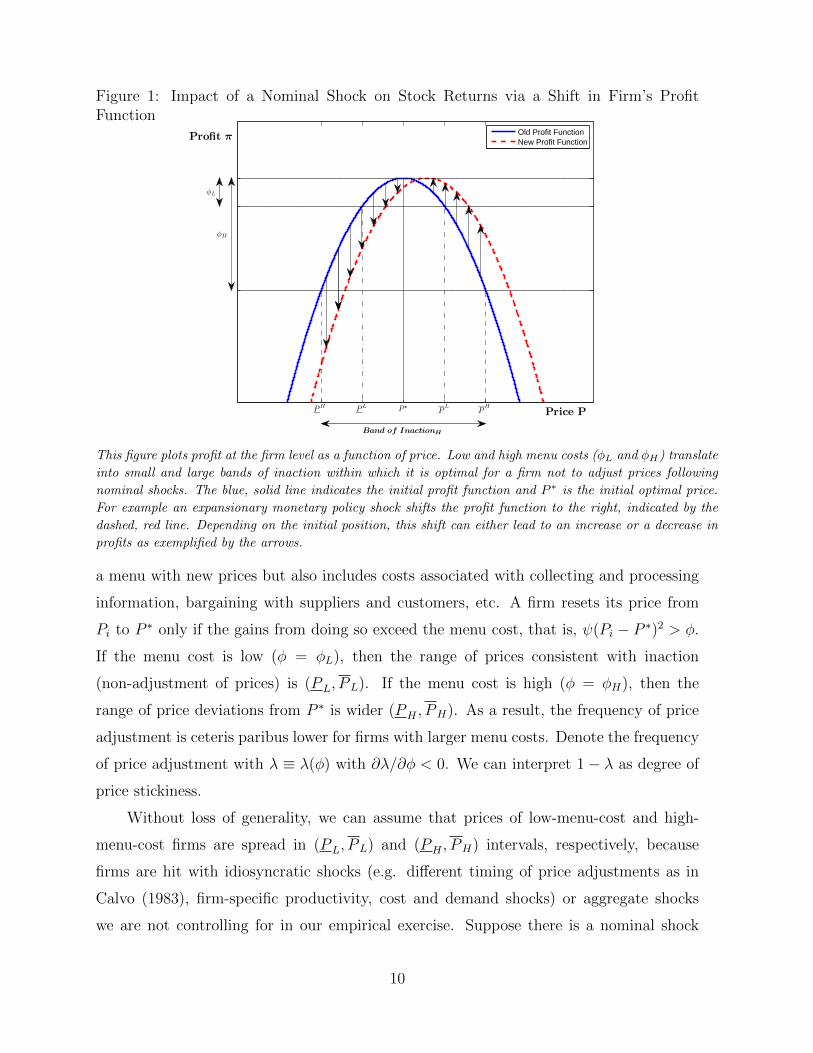
Figure 1: Impact of a Nominal Shock on Stock Returns via a Shift in Firm’s ProfitFunction

Price P

Profit π

PH PL P?P

LP

H

φL

φH

Band of InactionH

Old Profit FunctionNew Profit Function

Student Version of MATLAB

This figure plots profit at the firm level as a function of price. Low and high menu costs (φL and φH) translate

into small and large bands of inaction within which it is optimal for a firm not to adjust prices following

nominal shocks. The blue, solid line indicates the initial profit function and P ∗ is the initial optimal price.

For example an expansionary monetary policy shock shifts the profit function to the right, indicated by the

dashed, red line. Depending on the initial position, this shift can either lead to an increase or a decrease in

profits as exemplified by the arrows.

a menu with new prices but also includes costs associated with collecting and processing

information, bargaining with suppliers and customers, etc. A firm resets its price from

Pi to P ∗ only if the gains from doing so exceed the menu cost, that is, ψ(Pi − P ∗)2 > φ.

If the menu cost is low (φ = φL), then the range of prices consistent with inaction

(non-adjustment of prices) is (PL, PL). If the menu cost is high (φ = φH), then the

range of price deviations from P ∗ is wider (PH , PH). As a result, the frequency of price

adjustment is ceteris paribus lower for firms with larger menu costs. Denote the frequency

of price adjustment with λ ≡ λ(φ) with ∂λ/∂φ < 0. We can interpret 1− λ as degree of

price stickiness.

Without loss of generality, we can assume that prices of low-menu-cost and high-

menu-cost firms are spread in (PL, PL) and (PH , PH) intervals, respectively, because

firms are hit with idiosyncratic shocks (e.g. different timing of price adjustments as in

Calvo (1983), firm-specific productivity, cost and demand shocks) or aggregate shocks

we are not controlling for in our empirical exercise. Suppose there is a nominal shock

10

which moves P ∗ to the right (denote this new optimal price with P ∗new) so that the payoff

function is now described by the red, dashed line. This shift can push some firms outside

their inaction bands and they will reset their prices to P ∗new and thus weakly increase their

payoffs, (i.e. π(P ∗new, P∗new) − π(Pi, P

∗new) > φ). If the shock is not too large, many firms

will continue to stay inside their inaction bands.

Obviously, this non-adjustment does not mean that firms have the same payoffs after

the shock. Firms with negative (Pi−P ∗) will clearly lose (i.e. π(Pi, P∗new)−π(Pi, P

∗) < 0)

as their prices become even more suboptimal. Firms with positive (Pi−P ∗new) will clearly

gain (i.e. π(Pi, P∗new)−π(Pi, P

∗) > 0) as their suboptimal prices become closer to optimal.

Firms with positive (Pi−P ∗) and negative (Pi−P ∗new) may lose or gain. In short, a nominal

shock to P ∗ redistributes payoffs.

Note that there are losers and winners for both low-menu-cost and high-menu-cost

firms. In other words, if we observe an increased payoff, we cannot infer that this increased

payoff identifies a low-menu-cost firm. If we had information about (Pi − P ∗new) and/or

(Pi − P ∗), that is, relative prices of firms, then we could infer the size of menu costs

directly from price resets. It is unlikely that this information is available in a plausible

empirical setting as P ∗ is hardly observable.

Fortunately, there is an unambiguous prediction with respect to the variance of

changes in payoffs in response to shocks. Specifically, firms with high menu costs have

larger variability in payoffs than firms with low menu costs. Indeed, high-menu-cost firms

can tolerate a loss of up to φH in profits while low-menu-cost firms take at most a loss of

φL. This observation motivates the following empirical specification:

(∆πi)2 = b1 × v2 + b2 × v2 × λ(φi) + b3 × λ(φi) + error. (1)

where ∆πi is a change in payoffs (return) for firm i, v is a shock to the optimal price

P ∗, error absorbs movements due to other shocks. In this specification, we expect b1 >

0 because a shock v results in increased volatility of payoffs. We also expect b2 < 0

because the volatility increases less for firms with smaller bands of inaction and hence

with more flexible prices. Furthermore, the volatility of profits should be lower for low-

menu-cost firms unconditionally so that b3 < 0. In the polar case of no menu costs, there

is no volatility in payoffs after a nominal shock as firms always make πmax. Therefore,

we also expect that b1 + b2 ≈ 0. To simplify the exposition of the static model, we

11

implicitly assumed that nominal shocks do not move the profit function up or down. If

this assumption is relaxed, b1 + b2 can be different from zero. We do not make this

assumption in either the dynamic version of the model presented in Section V or our

empirical analyses. We find in simulations and in the data that b1 + b2 ≈ 0.

While the static model provides intuitive insights about the relationship between

payoffs and price stickiness, it is obviously not well suited for quantitative analyses

for several reasons. First, when firms decide whether to adjust their product prices

they compare the cost of price adjustment with the present value of future increases

in profits associated with adjusting prices. Empirically, we measure returns that capture

both current dividends/profits and changes in the valuation of firms. Since returns are

necessarily forward looking, we have to consider a dynamic model. Second, general

equilibrium effects may attenuate or amplify effects of heterogeneity in price stickiness

on returns. Indeed, strategic interaction between firms is often emphasized as the key

channel of gradual price adjustment in response to aggregate shocks. For example, in

the presence of strategic interaction and some firms with sticky prices, even flexible price

firms may be reluctant to change their prices by large amounts and thus may appear to

have inflexible prices (see e.g. Haltiwanger and Waldman (1991) and Carvalho (2006)).

Finally, the sensitivity of returns to macroeconomic shocks is likely to depend on the

cross-sectional distribution of relative prices which varies over time and may be difficult

to characterize analytically.

To address these concerns and check whether the parameter estimates in our empirical

analysis of Section IV are within reasonable ranges, we calibrate the dynamic multi-sector

model developed in Carvalho (2006) where firms are heterogeneous in the degree of price

stickiness in Section V.

B. Identification

Identification of unanticipated, presumably exogenous shocks to monetary policy

is central for our analysis. In standard macroeconomic contexts (e.g. structural

vector autoregressions), one may achieve identification by appealing to minimum delay

restrictions where monetary policy is assumed to be unable to influence the economy

(e.g. real GDP or unemployment rate) within a month or a quarter. However, asset

prices are likely to respond to changes in monetary policy within days if not hours or

minutes. Balduzzi et al. (2001) show for bonds and Andersen et al. (2003) for exchange

12

rates that announcement surprises are almost immediately incorporated into asset prices.

Furthermore, Rigobon and Sack (2003) show that monetary policy is systematically

influenced by movements in financial markets within a month. In short, stock prices and

monetary policy can both change following major macroeconomic news and can respond

to changes in each other even in relatively short time windows.

To address this identification challenge, we employ an event study approach in the

tradition of Cook and Hahn (1989) and more recently Kuttner (2001), Bernanke and

Kuttner (2005) and Gurkaynak et al. (2005). Specifically, we examine the behavior of

returns and changes in the Fed’s policy instrument in narrow time windows (30 minutes,

60 minutes, daily) around FOMC press releases. In these narrow time windows, the only

relevant shock (if any) is likely due to changes in monetary policy.

However, not every change in policy rates affects stock prices at the time of the

change. In informationally efficient markets, anticipated changes in monetary policy are

already incorporated into prices and only the surprise components of monetary policy

changes should matter for stock returns.16 To isolate the unanticipated part of the

announced changes of the target rate, we use federal funds futures which provide a

high-frequency market-based measure of the anticipated path of the fed funds rate. This

measure has a number of advantages: i) it allows for a flexible characterization of the

policy reaction function; ii) it can accommodate changes in the policy reaction function

of decision makers at the FOMC; and iii) it aggregates a vast amount of data processed by

the market. Krueger and Kuttner (1996) show that federal funds futures are an efficient

predictor of future federal funds rates. Macroeconomic variables such as the change

in unemployment rate or industrial production growth have no incremental forecasting

power for the federal funds rate once the federal funds futures is included in forecasting

regressions. In similar spirit, Gurkaynak et al. (2007) provide evidence that the federal

funds futures dominate other market based instruments in forecasting the federal funds

rate. In short, fed funds futures provides a powerful and simple summary of market

expectations for the path of future fed funds rates. Using this insight, we can calculate

16Bernanke and Kuttner (2005) perform a decomposition in expected and unexpected changes in thefederal funds target rate and indeed show that only the unanticipated component systematically movesthe stock market.

13

the surprise component of the announced change in the federal funds rate as:

vt =D

D − t(ff 0

t+∆t+ − ff 0t−∆t−) (2)

where t is the time when the FOMC issues an announcement, ff 0t+∆t+ is the fed funds

futures rate shortly after t, ff 0t−∆t− is the fed funds futures rate just before t, and D

is the number of days in the month.17 The D/(D − t) term adjusts for the fact that

the federal funds futures settle on the average effective overnight federal funds rate. We

follow Gurkaynak et al. (2005) and use the unscaled change in the next month futures

contract if the event day occurs within the last seven days of the month. This ensures

that small targeting errors in the federal funds rate by the trading desk at the New York

Fed, revisions in expectations of future targeting errors, changes in bid-ask spreads or

other noise, which have only a small effect on the current month average, is not amplified

through multiplication by a large scaling factor.

Using this shock series, we apply the following empirical specification to assess

whether price stickiness leads to differential responses of stock returns:

R2it = b0 + b1 × v2

t + b2 × v2t × λi + b3 × λi

+FirmControls+ FirmControls× v2t + error (3)

where R2it is the squared return of stock i in the interval [t−∆t−,t+ ∆t+] around event t,

v2t is the squared monetary policy shock and λi is the frequency of price adjustment of firm

i. Below, we provide details on how high frequency shocks and returns are constructed

and we briefly discuss properties of the constructed variables. Our identification does

not require immediate reaction of inflation to monetary policy shocks but can also

operate trough changes in current and future demand and costs which are immediately

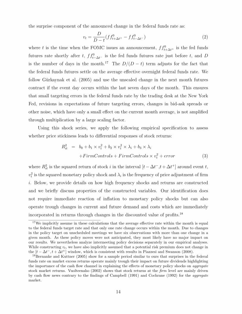
incorporated in returns through changes in the discounted value of profits.18

17We implicitly assume in these calculations that the average effective rate within the month is equalto the federal funds target rate and that only one rate change occurs within the month. Due to changesin the policy target on unscheduled meetings we have six observations with more than one change in agiven month. As these policy moves were not anticipated, they most likely have no major impact onour results. We nevertheless analyze intermeeting policy decisions separately in our empirical analyses.While constructing vt, we have also implicitly assumed that a potential risk premium does not change inthe [t−∆t−, t+ ∆t+] window, which is consistent with results in Piazzesi and Swanson (2008).

18Bernanke and Kuttner (2005) show for a sample period similar to ours that surprises in the federalfunds rate on market excess returns operate mainly trough their impact on future dividends highlightingthe importance of the cash flow channel in explaining the effects of monetary policy shocks on aggregatestock market returns. Vuolteenaho (2002) shows that stock returns at the firm level are mainly drivenby cash flow news contrary to the findings of Campbell (1991) and Cochrane (1992) for the aggregatemarket.

14

C. Data

We acquired tick-by-tick data of the federal funds futures trading on the Chicago

Mercantile Exchange (CME) Globex electronic trading platform (as opposed to the open

outcry market) directly from the CME. Using Globex data has the advantage that trading

in these contracts starts on the previous trading day at 6.30 pm ET (compared to 8.20am

ET in the open outcry market). We are therefore able to calculate the monetary policy

surprises for all event days including the intermeeting policy decisions occurring outside of

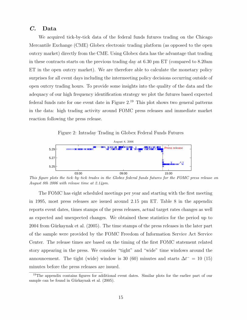
open outcry trading hours. To provide some insights into the quality of the data and the

adequacy of our high frequency identification strategy we plot the futures based expected

federal funds rate for one event date in Figure 2.19 This plot shows two general patterns

in the data: high trading activity around FOMC press releases and immediate market

reaction following the press release.

Figure 2: Intraday Trading in Globex Federal Funds Futures

03:00 09:00 15:00

5.25

5.27

5.29 Press release

August 8, 2006

03:00 09:00 15:00

4.85

4.95

5.05 Press release

September 18, 2007

03:00 09:00 15:00

2.55

2.60

2.65Press release

March 18, 2008

This figure plots the tick–by–tick trades in the Globex federal funds futures for the FOMC press release on

August 8th 2006 with release time at 2.14pm.

The FOMC has eight scheduled meetings per year and starting with the first meeting

in 1995, most press releases are issued around 2.15 pm ET. Table 8 in the appendix

reports event dates, times stamps of the press releases, actual target rates changes as well

as expected and unexpected changes. We obtained these statistics for the period up to

2004 from Gurkaynak et al. (2005). The time stamps of the press releases in the later part

of the sample were provided by the FOMC Freedom of Information Service Act Service

Center. The release times are based on the timing of the first FOMC statement related

story appearing in the press. We consider “tight” and “wide” time windows around the

announcement. The tight (wide) window is 30 (60) minutes and starts ∆t− = 10 (15)

minutes before the press releases are issued.

19The appendix contains figures for additional event dates. Similar plots for the earlier part of oursample can be found in Gurkaynak et al. (2005).

15

Panel A of Table 2 reports descriptive statistics for surprises in monetary policy

for all 137 event dates between 1994 and 2009 as well as separately for turning points in

monetary policy and intermeeting policy decisions. Turning points are target rate changes

in the direction opposite to previous changes. Jensen et al. (1996) argue that the Fed is

operating under the same fundamental monetary policy regime until the first change in

the target rate in the opposite direction. This is in line with the observed level of policy

inertia and interest rate smoothing (cf Piazzesi (2005) and Coibion and Gorodnichenko

(2012) as well as Figure 2 in the appendix). Monetary policy reversals therefore contain

valuable information on the future policy stance.

The average monetary policy shock is approximately zero. The most negative shock

is with more than -45 bps about three times larger in absolute value than the most positive

shock. Policy surprises on intermeeting event dates and turning points are more volatile

than surprises on scheduled meetings. Andersen et al. (2003) point out that financial

markets react differently on scheduled versus non-scheduled announcement days. Lastly,

the monetary policy shocks are almost perfectly correlated across the two event windows

(see Figure 3 in the appendix).20

We sample returns for all constituents of the S&P500 for all event dates. We use the

CRSP database to obtain the constituent list of the S&P500 for the respective event date

and link the CRSP identifier to the ticker of the NYSE taq database via historical CUSIPs

(an alphanumeric code identifying North American securities). NYSE taq contains all

trades and quotes for all securities traded on NYSE, Amex and the Nasdaq National

Market System. We use the last observation before the start of the event window and

the first observations after the end of the event window to calculate event returns. We

manually checked all event returns which are larger than 5% in absolute value for potential

data entry errors in the tick-by-tick data. For the five event dates for which the press

releases were issued before start of the trading session (all intermeeting releases in the

easing cycle starting in 2007, see Table 8 in the appendix) we calculate event returns using

20Only two observations have discernible differences: August 17, 2007 and December 16, 2008 . Thefirst observation is an intermeeting event day on which the FOMC unexpectedly cut the discount rateby 50 bps at 8.15am ET just before the opening of the open-outcry futures market in Chicago. Thefinancial press reports heavy losses for the August futures contract on that day and a very volatilemarket environment. The second observation, December 16, 2008, is the day on which the FOMC cutthe federal funds rate to a target range between zero and 0.25 percent.

16

closing prices of the previous trading day and opening prices of the event day.21

Our sample period ranges from February 2, 1994, the first FOMC press release in

1994, to December 16, 2009, the last announcement in 2009 for a total of 137 FOMC

meetings. We exclude the rate cut of September 17, 2001—the first trading day after the

terrorist attacks of September 11, 2001. Our sample starts in 1994 as our tick-by-tick stock

price data is not available before 1993 and the FOMC changed the way it communicated

its policy decisions. Prior to 1994, the market became aware of changes in the federal

funds target rate through the size and the type of open market operations of the New

York Fed’s trading desk. Moreover, most of the changes in the federal funds target rate

took place on non-meeting days. With the first meeting in 1994, the FOMC started to

communicate its decision by issuing press releases after every meeting and policy decision.

Therefore, the start of our sample eliminates almost all timing ambiguity (besides the nine

intermeeting policy decisions). The increased transparency and predictability makes the

use of our intraday identification scheme more appealing as our identification assumptions

are more likely to hold.

Panel B of Table 2 reports descriptive statistics for the percentage returns of the

S&P500 for all 137 event dates between 1994 and 2009, turnings points and intermeeting

policy decisions. We use the event returns of the 500 firms comprising the S&P500 to

calculate index returns using the market capitalization at the end of the previous trading

day as weights. The average return is close to zero with an event standard deviation of

about one percent. The large absolute values of the tight (30 minute) and wide (60 minute)

event returns are remarkable. Looking at the columns for intermeeting press releases

and turning points, we see that the most extreme observations occur on non-regular

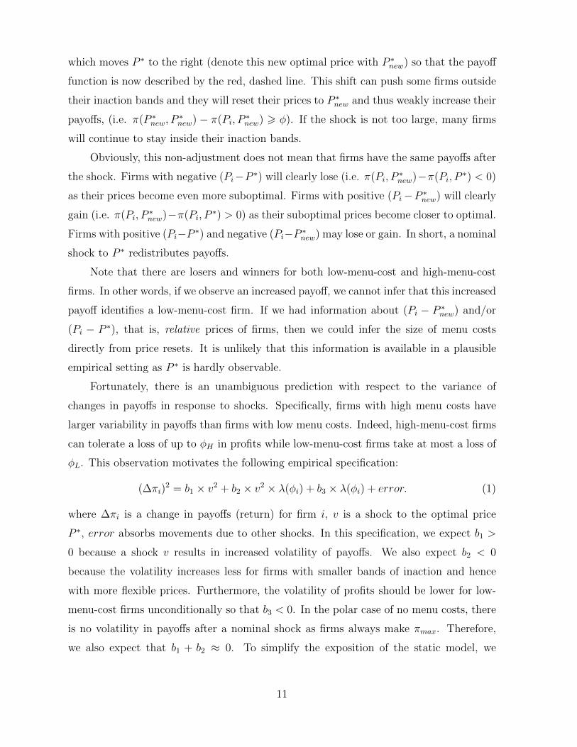
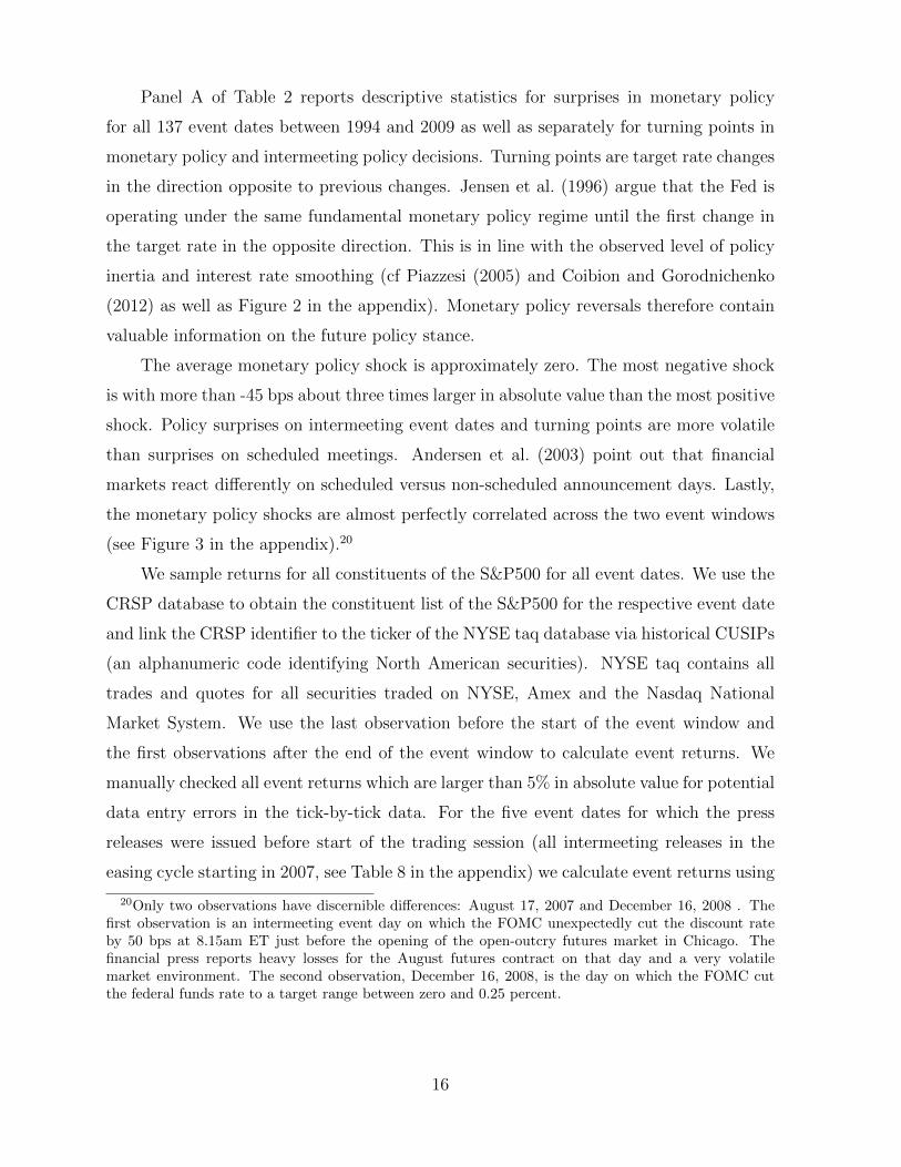
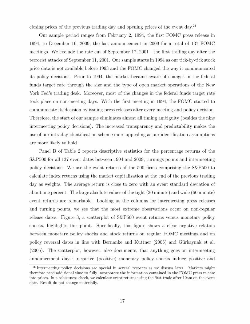
release dates. Figure 3, a scatterplot of S&P500 event returns versus monetary policy

shocks, highlights this point. Specifically, this figure shows a clear negative relation

between monetary policy shocks and stock returns on regular FOMC meetings and on

policy reversal dates in line with Bernanke and Kuttner (2005) and Gurkaynak et al.

(2005). The scatterplot, however, also documents, that anything goes on intermeeting

announcement days: negative (positive) monetary policy shocks induce positive and

21Intermeeting policy decisions are special in several respects as we discuss later. Markets mighttherefore need additional time to fully incorporate the information contained in the FOMC press releaseinto prices. In a robustness check, we calculate event returns using the first trade after 10am on the eventdate. Result do not change materially.

17

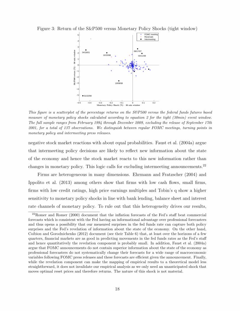
Figure 3: Return of the S&P500 versus Monetary Policy Shocks (tight window)

−0.5 −0.4 −0.3 −0.2 −0.1 0 0.1 0.2

−5

−4

−3

−2

−1

0

1

2

3

4

5

Monetary Policy Shock (%) – 30 min window

S&P500retu

rn(%

)–30min

window

10/15/9804/18/01

08/17/07

01/22/08

03/11/08

10/08/08

FOMC meetingReversalsIntermeeting

Student Version of MATLAB

This figure is a scatterplot of the percentage returns on the S&P500 versus the federal funds futures based

measure of monetary policy shocks calculated according to equation 2 for the tight (30min) event window.

The full sample ranges from February 1994 through December 2009, excluding the release of September 17th

2001, for a total of 137 observations. We distinguish between regular FOMC meetings, turning points in

monetary policy and intermeeting press releases.

negative stock market reactions with about equal probabilities. Faust et al. (2004a) argue

that intermeeting policy decisions are likely to reflect new information about the state

of the economy and hence the stock market reacts to this new information rather than

changes in monetary policy. This logic calls for excluding intermeeting announcements.22

Firms are heterogeneous in many dimensions. Ehrmann and Fratzscher (2004) and

Ippolito et al. (2013) among others show that firms with low cash flows, small firms,

firms with low credit ratings, high price earnings multiples and Tobin’s q show a higher

sensitivity to monetary policy shocks in line with bank lending, balance sheet and interest

rate channels of monetary policy. To rule out that this heterogeneity drives our results,

22Romer and Romer (2000) document that the inflation forecasts of the Fed’s staff beat commercialforecasts which is consistent with the Fed having an informational advantage over professional forecastersand thus opens a possibility that our measured surprises in the fed funds rate can capture both policysurprises and the Fed’s revelation of information about the state of the economy. On the other hand,Coibion and Gorodnichenko (2012) document (see their Table 6) that, at least over the horizons of a fewquarters, financial markets are as good in predicting movements in the fed funds rates as the Fed’s staffand hence quantitatively the revelation component is probably small. In addition, Faust et al. (2004a)argue that FOMC announcements do not contain superior information about the state of the economy asprofessional forecasters do not systematically change their forecasts for a wide range of macroeconomicvariables following FOMC press releases and these forecasts are efficient given the announcement. Finally,while the revelation component can make the mapping of empirical results to a theoretical model lessstraightforward, it does not invalidate our empirical analysis as we only need an unanticipated shock thatmoves optimal reset prices and therefore returns. The nature of this shock is not material.

18

we control for an extended set of variables at the firm and industry level. For example,

we construct measures of firm size, volatility and cyclical properties of demand, market

power, cost structure, financial dependence, access to financial markets, etc. We use

data from a variety of sources such as the Standard and Poor’s Compustat database,

publications of the U.S. Census Bureau, and previous studies. The appendix contains

detailed information on how these variables are measured.

IV Empirical Results

A. Aggregate Market Volatility

We first document the effects of monetary policy shocks on the return of the aggregate

market to ensure that these shocks are a meaningful source of variation. Table 3 reports

results from regressing returns of the S&P500 on monetary policy surprises as well as

squared index returns on squared policy shocks for our tight event window (30 min).23

Column (1) shows that a higher than expected federal funds target rate leads to a drop

in stocks prices. This effect—contrary to findings in the previous literature—is not

statistically significant. Restricting our sample period to 1994-2004 (or 1994-2007), we

can replicate the results of Bernanke and Kuttner (2005), Gurkaynak et al. (2005), and

others: a 25 bps unexpected cut in interest rates leads to an increase of the S&P500 by

more than 1.3%. In column (3), we find a highly statistically significant impact of squared

policy shocks on squared index returns. Conditioning on different types of meetings shows

that the overall effect is mainly driven by turning points in monetary policy. Widening the

event window mainly adds noise, increasing standard errors and lowering R2s, but does

not qualitatively alter the results (see appendix). In summary, monetary policy surprises

are valid shocks for our analysis.

B. Baseline

Panel A of Table 4 presents results for the baseline specification (3) where we regress

squared event returns at the firm level on the squared policy surprise, the frequencies of

price adjustments and their interactions. To account for correlation of error terms across

23Table 2 in the online appendix contains results both for the 30 minutes event window in columns (1)to (6) as well as the 60 minutes event window in columns (7) to (12).

19

time and firms, we report Driscoll and Kraay (1998) standard errors in parentheses.24

Column (1) of Panel A. shows that squared surprises have a large positive impact

on squared stocks returns. The point estimate is economically large and statistically

significant at the 1% level: a hypothetical policy surprise of 25 bps leads to an increase

in squared returns of roughly 8%2 (0.252 × 128.50 = 8.03). The estimated coefficient

on the interaction of the frequency of price adjustment and the squared shock indicates

that this effect is lower for firms with more flexible prices. For the firms with the most

flexible prices in our sample (which have a probability of price adjustment of roughly 0.5

per month), the impact of squared monetary policy shocks is reduced by a factor of three,

that is, (β1 − 0.5 × β3)/β1 ≈ 1/3. Importantly, this sensitivity is broadly in line with

the estimates we obtain for simulated data from a calibrated New Keynesian model (see

Section V.).

The differential response of conditional volatility for sticky and flexible price firms

is a very robust result. Controlling for outliers (column (2)),25 adding firm fixed effects

(columns (3) and (4)), firm and event (time) fixed effects (columns (5) and (6)), or looking

at a 60 minutes event window (columns (7) and (8)) does not materially change point

estimates and statistical significance for the interaction term between squared policy

surprises and the frequency of price adjustment. Increasing the observation period to

a daily event window (columns (9) and (10)) adds a considerable amount of noise,

reducing explanatory power and increasing standard errors. Point estimates are no longer

statistically significant but they remain economically large and relative magnitudes are

effectively unchanged. This pattern is consistent with Bernanke and Kuttner (2005) and

Gurkaynak et al. (2005) who document that for the aggregate market that R2s are reduced

by a factor of 3 and standard errors increase substantially as the event window increases

to the daily frequency.26

While in the baseline measurement of stock returns we use only two data ticks, we

24Note that we have 956 unique firms in sample due to changes in the index composition during oursample period out of which we were able to merge 760 with the BLS pricing data.

25We use a standard approach of identifying outliers by jackknife as described in Belsley, Kuh, andWelsch (1980) and Bollen and Jackman (1990).

26While the effects for the aggregate market can be explained by additional macro announcementsor stock market relevant news, many more stock price relevant news can be observed for individualstocks such as earning announcements, analyst reports, management decisions etc. rationalizing thelarge increase in standard errors. Rigobon and Sack (2004) and Gurkaynak and Wright (2013) alsohighlight that intraday event windows are more well suited from an econometric point of view as dailyevent windows might give rise to biased estimates.

20

find very similar results (Panel B. columns (1) and (2)) when we weight returns by trade

volume in time windows before and after our events. The results also do not change

qualitatively when we use absolute returns and policy shocks (columns (3) and (4) of

Panel B.) instead of squared returns and squared shocks.

One may be concerned that the heterogeneity in volatility across firms is largely driven

by market movements or exposure to movements of other risk factors rather than forces

specific to the price stickiness of particular firms. To address this concern, we consider

squared market-adjusted returns (i.e. (Rit − RSPt )2), squared CAPM-adjusted returns

(i.e. (Rit − βiRSPt )2), and squared Fama-French-adjusted returns ((Rit − βiFFR

FFt )2)

where βi and βiFF are time series factor loadings of the excess returns of firm i on the

market excess returns and the three Fama-French factors. All three adjustments (Panel

B.: columns (5) and (6), columns (7) and (8), and columns (9) and (10)) take out a lot

of common variation, reducing both explanatory power and point estimates somewhat

but leaving statistical significance and relative magnitudes unchanged or even increasing

it slightly. Thus, conditional volatility responds differentially across firms even after we

adjust for movements of the aggregate market and other risk factors which itself could be

influenced by nominal rigidities as no firm in our sample has perfectly flexible prices.

The sensitivity of the conditional volatility to monetary policy shocks may vary across

types of events. For example, Gurkaynak et al. (2005) and others show that monetary

policy announcements about changes in the path/direction of future policy are more

powerful in moving markets. Panel C. of Table 4 contains results for different event

types. We restrict our sample in columns (3) and (4) to observations before 2007 to

control for the impact of the Great Recession and the zero lower bound. The effect of

price flexibility increases both statistically and economically in the restricted sample. In

the next two columns, we follow Bernanke and Kuttner (2005) and restrict the sample

only to episodes when the FOMC changed the policy interest rate. While this reduces

our sample size by more than 50%, it has no impact on estimated coefficients. Some

of the monetary policy shocks are relatively small. To ensure that the large effects of

price rigidity are not driven by these observations, we restrict our sample to events with

shocks larger than 0.05 in absolute value in columns (7) and (8). Both for the full and the

no outliers samples, statistical and economic significance remains stable or even slightly

increases. The next column conditions on reversals in monetary policy (i.e. turning

21

points in policy). The coefficient on the interaction term between the probability of price

adjustment and squared policy shocks increases by a factor of three. The effect of policy

shocks is somewhat reduced for intermeeting releases as shown in the last column.

C. Additional controls and subsamples

In Table 5, we add a wide range of controls to disentangle the effect of price stickiness

from potentially confounding firm and industry effects. In the first column we repeat the

baseline regression excluding outliers. In the first set of controls, we focus on measures

of market power and profitability. For example, in column (2) we include the squared

shock interacted with the price cost margin (pcm) as an additional regressor. While firms

with larger pcm appear to have volatility more sensitive to monetary policy shocks, the

sensitivity of the volatility across firms with different frequencies of price adjustment is

barely affected by including pcm. Likewise, controlling directly for market power with

industry concentration (the share of sales by the four largest firms, 4F − conc ratio,

column (3)) does not change our main result. We also find that our results for b2 in

equation (3) do not alter when we control for the book to market ratio (column (4)) or

firm size (column (5)).27

The differential sensitivity of volatility across sticky and flexible price firms may arise

from differences in the volatility of demand for sticky and flexible price firms. For example,

all firms could face identical menu costs but firms which are hit more frequently by

idiosyncratic shocks have a higher frequency of price adjustment and hence may be closer

to their optimal reset prices which in turn entails that they could have a lower sensitivity

to nominal shocks. To disentangle this potentially confounding effect, we explicitly control

for the volatility of sales (standard deviation of sales growth rates, std sale,28 column (6))

and for durability of output (columns (7) and (8)) using the classifications of Gomes et al.

(2009) and Bils et al. (2012), respectively. The latter control is important as demand

for durable goods is particularly volatile over the business cycle and consumers can easily

shift the timing of their purchases thus making price sensitivity especially high. Even with

27Note that the coefficient on the squared policy surprise now turns negative. This coefficient, however,can no longer be as easily interpreted as before in the presence of additional control variables. If we reportresults evaluating additional controls at their mean level, coefficients are similar in size to our benchmarkestimation.

28We use the standard deviation of annual sales growth at the quarterly frequency to control forseasonality in sales. Ideally, we would want to have higher frequency data to construct this variable butpublicly available sources only contain sales at the quarterly frequency.

22

these additional regressors, we find that the estimated differential sensitivity of volatility

across sticky and flexible price firms is largely unchanged.

Some heterogeneity of stickiness in product prices may reflect differences in the

stickiness of input prices. For example, labor costs are often found to be relatively

inflexible due to rigid wages. In column (9), we control for input price stickiness proxied

by the share of labor expenses in sales and we indeed find that firms with a larger

share of labor cost have greater sensitivity to monetary policy shocks. This additional

control however does not affect our estimates of how stickiness of product prices influences

conditional volatility of returns. In columns (10) to (18), we additionally control for fixed

costs to sales (FC2Y ) as a higher ratio might decrease the flexibility to react to monetary

policy shocks, receivables minus payables to sales ratio (RecPay2Y ) to control for the

impact of short term financing, investment to sales ratio (I2Y ) to control for investment

opportunities, depreciation to assets ratio (D2A) as a measure of capital intensity, the

rate of synchronization in price adjustments within a firm (sync), the number of products

at the firm level (#prod) as well as the S&P long term issuer rating (Rat) and the Kaplan

- Zingales index (KZ) to investigate the impact of financial constraints. Overall, none

of the controls—neither individually nor jointly—attenuates the effect of price stickiness

which is highly statistically and economically significant.

In Panel A. of Table 6 we run our baseline regression at the industry level to control

for possible unobserved industry heterogeneity. In this exercise, we have typically much

fewer firms and thus estimates have higher sampling uncertainty. Despite large reductions

in sample sizes, for four out of the six industries we find a statistically significant

negative coefficient on the interaction term between the frequency of price adjustment

and squared monetary policy surprises. For the finance industry, this coefficient is not

statistically significant. For the service sector, the estimate for the full sample is positive

and significant but this result is driven by a handful of outliers. Once these outliers

are removed, the point estimate becomes much smaller and statistically insignificantly

different from zero. This test uses only variation of our measure of price stickiness within

industry. We see these results as comforting insofar as they document that our baseline

effects are not driven by unobserved industry characteristics.

An alternative possibility which could drive our results is a general return sensitivity

to monetary policy surprises independent of price stickiness. To rule out that this

23

alternative explanation, we directly add the return sensitivity to monetary policy shocks.29

To perform this test we first estimate the sensitivity (βvt) by regressing firm-level event

returns on monetary policy shocks in our narrow event window. Then we add the return

sensitivity interacted with the squared monetary policy surprise in various specifications

as an additional control variable in our baseline regression. Panel B. of Table 6 shows

that a higher squared return sensitivity to monetary policy surprises indeed leads to an

increase in event return volatilities but this additional control has a negligible effect on the

interaction term of our measure of price stickiness and squared monetary policy shocks.

D. Relative Volatility and Placebo Test

In this subsection, we perform two additional economically motivated robustness

checks to further examine potentially confounding unobserved firm heterogeneity: one in

which price stickiness should matter and one where we do not expect to find an effect of

price stickiness.

Specifically, the first check is built on the idea that if inflexible price firms have

unconditionally higher volatility than flexible price firms and this drives the previously

documented effects, then we should find no effects of price stickiness once we scale the

event volatilities by their unconditional volatilities. To implement this test, we pick

a pseudo event window in the middle of two adjacent event dates t and t − 1 (date

τ = t − 1/2) and calculate a pseudo event volatility (1 + Riτ )2 in a 30 minute window

bracketing 2.15pm at date τ . We then scale the event volatilities of the following event

date with these volatilities, (1 + Rit)2/(1 + Riτ )

2, and run our baseline regression with

(1 +Rit)2/(1 +Riτ )

2 as the dependent variable.

Column (1) in Panel A. of Table 7 shows that this story cannot explain our result that

flexible price firms have lower conditional volatilities than sticky price firms. Monetary

policy surprises increase event volatility compared to non-event dates. This conditional

increase is completely offset for the most flexible firms with both coefficients being highly

statistically significant. Controlling for outliers in column (2), firm fixed effects, event

fixed effects or both in columns (3) to (8) does not change this conclusion.

The second check is aimed to address the concern that unobserved heterogeneity can

drive our results is to directly run our baseline regression on the pseudo event volatilities.

We perform this test in Panel B. of Table 7: all coefficients are economically small,

29We thank David Romer for suggesting this test.

24

none of them is statistically significant and once we exclude outliers, the coefficient on

the interaction term between the monetary policy surprise and the frequency of price

adjustment changes sign.

E. Profits

The large differential effects of price stickiness on the volatility of returns suggest that

firms with inflexible prices should experience an increased volatility of profits relative

to firms with flexible prices. This response in fundamentals may be difficult to detect

as information on firm profits is only available at quarterly frequency. To match this

much lower frequency, we sum shocks vt in a given quarter and treat this sum as the

unanticipated shock. Denote this shock with vt. We also construct the following measure

of change in profitability between the previous four quarters and quarters running from

t+H to t+H + 3:

∆πit,H =14

∑t+H+3s=t+H OIis −

14

∑t−1s=t−4OIis

TAit−1

× 100 (4)

where OI is quarterly operating income before depreciation, TA is total assets, and H can

be interpreted as the horizon of the response. We use four quarters before and after the

shock to address seasonality of profits. Using this measure of profitability, we estimate

the following modification of our baseline specification:

(∆πit,H)2 = b0 + b1 ×∆v2t + b2 × v2

t × λi + b3 × λi + error (5)

We find (Table 8) that flexible price firms have a statistically lower volatility in

operating income than sticky price firms (b2 < 0). This effect is increasing up to H = 6

quarters ahead and then this difference becomes statistically insignificant and gradually

converges to zero. Firms with more inflexible prices (smaller FPA) tend to have larger

volatilities of profits. Interestingly, the estimate of b1 is statistically positive only at H = 0

and turns statistically negative after H = 5.

V Dynamic General Equilibrium Model

While the static version of the New Keynesian model in section III was useful in

guiding our empirical specifications it is not well suited for a quantitative analysis. To

assess whether our empirical findings can be rationalized by a dynamic multi-sector

New Keynesian model we calibrate the Carvalho (2006) model and run our baseline

25

specification on simulated data from the model.

In the interest of space, we only verbally discuss the model and focus on key

equations.30 In this model, a representative household lives forever. The instantaneous

utility of the household depends on consumption and labor supply. The intertemporal

elasticity of substitution for consumption is σ. Labor supply is firm-specific. For each

firm, the elasticity of labor supply is η. Household’s discount factor is β. Households

have a love for variety and have a CES Dixit-Stiglitz aggregator with the elasticity of

substitution θ.

Firms set prices as in Calvo (1983). There are k sectors in the economy with each

sector populated by a continuum of firms. Each sector is characterized by a fixed λk, the

probability of any firm in industry k to adjust its price in a given period.31 The share of

firms in industry k in the total number of firms in the economy is given by the density

function f(k). Firms are monopolistic competitors and the elasticity of substitution θ

is the same for all firms both within and across industries. While this assumption is

clearly unrealistic, it greatly simplifies the algebra and keeps the model tractable. The

production function for output Y is linear in labor N which is the only input. The

optimization problem of firm j in industry k is then to pick a reset price Xjkt:

maxEt∞∑s=0

Qt,t+s(1− λk)s[XjktYjkt+s −Wjkt+sNjkt+s] (6)

subject to its demand function and production technology where variables without

subscripts k and j indicate aggregate variables, W is wages (taken as given by firms) and Q

is the stochastic discount factor. Wages are determined by the household’s intratemporal

elasticity between labor and consumption. The central bank follows a Taylor rule.

After substituting in optimal reset prices and firm-specific demand and wages, the

value of the firm V with price Pjkt is given by:

V (Pjkt) = Et{Y σt Pt

[∆

(1)kt

(PjktPt

)1−θ

−∆(2)kt

(PjktPt

)−θ(1+1/η)

+ Υ(1)kt −Υ

(2)kt

]}, (7)

where Υ(1)kt , ∆

(1)kt , Υ

(2)kt and ∆

(2)kt follow simple recursions and are not indexed by j, which

allows particularly easy solution and simulation of this non-linear model.

30The appendix contains a more detailed description of the model.31The fixed probability of price adjustment should be interpreted as a metaphor that allows particularly

fast non-linear solutions to multi-sector models with large state spaces as well as easy interpretation ofresults. However we find similar results in the Dotsey et al. (1999) model with state-dependent priceadjustment. Results are available upon request.

26

We calibrate the model at quarterly frequency using standard parameter values in

the literature (Table 9). Ashenfelter et al. (2010) survey the literature on the elasticity of

labor supply faced by firms. They document that the short-run elasticity is in the 0.1-1.5

range while the long-run elasticity is between 2 and 4. We take the middle of the range

of these elasticities and set η = 2. The elasticity of demand θ is often calibrated at 10 in

macroeconomic studies. However, since firms in our model compete not only with firms in

the same sector but also with firms in other sectors we calibrate θ = 7 which captures the

notion that the elasticity of substitution across sectors is likely to be low. Other preference

parameters are standard: σ = 2 and β = 0.99. Parameters of the policy reaction function

are taken from Taylor (1993) and Coibion and Gorodnichenko (2012). We follow Carvalho

(2006) and calibrate the density function f(k) = 1/5 and use the empirical distribution of

frequencies of price adjustment reported in Nakamura and Steinsson (2008) to calibrate

{λk}5k=1. Specifically, we sort industries by the degree of price stickiness and construct

five synthetic sectors which correspond to the quintiles of price stickiness observed in

the data. Each sector covers a fifth of consumer spending. The Calvo rates of price

adjustment range from 0.094 to 0.975 per quarter with the median sector having a Calvo

rate of 0.277 (which implies that this sector updates prices approximately once a year).

We solve the model using a third-order approximation as implemented in DYNARE

and simulate the model for 100 firms per sector for 2000 periods, but discard the first

1000 periods as burn-in. For each firm and each time period, we calculate the value of the

firm V (Pjkt) and the value of the firm net of dividend V (Pjkt) ≡ V (Pjkt)− (PjktYjkt+s −Wjkt+sNjkt+s) as well as the implied return Rjkt = V (Pjkt)/V (Pjkt−1)−1. As we discussed

in the case of the static model, realized returns can increase or decrease in response to a

nominal shock. Hence, we consider the specification suggested previously:

R2jkt = b0 + b1 × v2

t + b2 × v2t × λj + b3 × λj + error (8)

We report resulting estimates of b1, b2 and b3 in Table 9 for the baseline calibration

as well as for alternative parametrizations. We find that a large, positive b1 and a large,

negative b2 are very robust features of the model with estimates in the ballpark of our

empirical findings in Section IV. Magnitudes of the coefficients are such that b1 + b2 ≈ 0.

The estimates of b3 are negative, as predicted, but generally close to zero.

We can also use this model to calculate lost profits due to price stickiness: we compute

27

the median profit πk for each firm type k and then use (πk − π5)/π5 to assess how an

increase in the duration of price spells from (1/λ5) (the sector with practically flexible

prices) to (1/λk) influences profits. We find that going from flexible prices to prices fixed

for roughly one year (sector 3) reduces profits by about 25%. While in the model the only

source of firm heterogeneity is the duration of price spells and thus differences in profits

can be attributed to price stickiness, the duration of price spells in the data is affected by

heterogeneous costs and benefits of price adjustment so that the mapping of lost profits

to the size of menu costs is likely to be complex. However, the magnitudes we observe in

our simulations appear broadly in line with those observed in the data. Zbaracki et al.

(2004) show that a manufacturing firm with an average duration of price spells of one

year spends about 20 percent of its net profit margin on nominal price adjustment.

Obviously, these calculations of menu-cost estimates depend of structural parameters

of the model. One may use empirical moments to infer these structural parameters. The

answer in this exercise is likely to depend on the details of the model, which can limit the

robustness. However, these simulations highlight the relationship between price stickiness

and returns and provides a sense of magnitudes one may expect in a reasonably calibrated

New Keynesian model with heterogeneous firms.

VI Concluding Remarks

Are sticky prices costly? We propose a simple framework to address this

question using the conditional volatility of stock market returns after monetary policy

announcements. We document that the conditional volatility rises more for firms with

stickier prices than for firms with more flexible prices. This differential reaction is

economically and statistically large as well as strikingly robust to a broad spectrum of

checks. This result suggests that menu costs—broadly defined to include physical costs

of price adjustment, informational frictions, etc.—are an important factor for nominal

price rigidity. Our empirical evidence lends support to the New Keynesian interpretation

of the observed nominal price rigidity at the microlevel: sticky prices are costly. Our

results are qualitatively and, under plausible calibrations, quantitatively consistent with

New Keynesian macroeconomic models where firms have heterogeneous price stickiness.

Our “model-free” evidence unambiguously suggests that sticky prices are indeed costly

for firms, which is consistent with the tenets of New Keynesian macroeconomics.

28

Our results have a number of policy implications. First, our findings provide

foundations for policy-workhorse macroeconomic models such as Christiano et al. (2005)

in which nominal frictions play a prominent role. Second, increasing trend inflation—a

policy suggested by a number of economists to combat deflationary spirals in the Great

Recessions—has possibly non-negligible costs in the light of our results. Third, the

presence of sticky prices is likely to generate larger fiscal multipliers (especially in times

of a binding zero lower bound on interest rates, see Christiano et al. (2011)) and thus

potentially justifies more activist fiscal policy aimed at stabilizing business cycles. Finally,

as emphasized by Bernanke and Kuttner (2005), monetary policy can influence the

economy via changes in asset prices and our results can provide a new perspective on

this channel as well as highlight its distributional aspects.

The high-frequency identification of causal effects of monetary shocks on the volatility

of stock returns suggests that connecting stock returns and measures of price stickiness

is a fruitful avenue for future research. For example, Weber (2013) studies how firm-level

and portfolio returns vary with measured price stickiness which can provide a simple

metric of the size of menu costs and shed new light on the sources of the cross-sectional

distribution of returns. Alternatively, one may integrate asset prices into fully fledged

DSGE models to obtain structural estimates of menu costs. We anticipate that using

information on stock returns in conjunction with firm-level measures of price stickiness

can help to discriminate between alternative models explaining the large real effect of

monetary policy with moderate degrees of price stickiness and the inertial reaction of

inflation, improve our understanding of how to price securities, and further bridge finance

and macroeconomics.

29

References

Andersen, T. G., T. Bollerslev, F. X. Diebold, and C. Vega (2003). Micro effects of macroannouncements: Real-time price discovery in foreign exchange. American EconomicReview 93 (1), 38–62.

Anderson, E., N. Jaimovich, and D. Simester (2012). Price stickiness: Empirical evidenceof the menu cost channel. Unpublished Manuscript, Northwestern University .

Ashenfelter, O. C., H. Farber, and M. R. Ransom (2010). Labor market monopsony.Journal of Labor Economics 28 (2), 203–210.

Balduzzi, P., E. J. Elton, and T. C. Green (2001). Economic news and bond prices:Evidence from the U.S. treasury market. The Journal of Financial and QuantitativeAnalysis 36 (4), 523–543.

Berger, D. and J. Vavra (2013). Dynamics of the u.s. price distribution. Unpublishedmanuscript, University of Chicago.

Bernanke, B. S. and K. N. Kuttner (2005). What explains the stock market’s reaction toFederal Reserve policy? The Journal of Finance 60 (3), 1221–1257.

Bhattarai, S. and R. Schoenle (2012). Multiproduct firms and price-setting: Theory andevidence from US producer prices. Unpublished manuscript, Brandeis University .

Bils, M. and P. J. Klenow (2004). Some evidence on the importance of sticky prices.Journal of Political Economy 112 (5), 947–985.

Bils, M., P. J. Klenow, and B. A. Malin (2012). Testing for Keynesian labor demand. InNBER Macroeconomics Annual 2012, forthcoming.

Blinder, A. S. (1991). Why are prices sticky? Preliminary results from an interview study.American Economic Review 81 (2), 89–96.

Bloom, N. (2009). The impact of uncertainty shocks. Econometrica 77 (3), 623–685.

Bomfim, A. N. (2003). Pre-announcement effects, news effects, and volatility: Monetarypolicy and the stock market. Journal of Banking & Finance 27 (1), 133–151.

Calvo, G. A. (1983). Staggered prices in a utility-maximizing framework. Journal ofMonetary Economics 12 (3), 383–398.

Campbell, J. Y. (1991). A variance decomposition for stock returns. The EconomicJournal 101 (405), 157–179.

Carvalho, C. (2006). Heterogeneity in price stickiness and the real effects of monetaryshocks. The B.E. Journal of Macroeconomics 2 (1), 1.

Christiano, L., M. Eichenbaum, and S. Rebelo (2011). When is the government spendingmultiplier large? Journal of Political Economy 119 (1), 78 – 121.

Christiano, L. J., M. Eichenbaum, and C. L. Evans (2005). Nominal rigidities and thedynamic effects of a shock to monetary policy. Journal of Political Economy 113 (1),1–45.

Cochrane, J. H. (1992). Explaining the variance of price-dividend ratios. Review ofFinancial Studies 5 (2), 243–280.

Coibion, O. and Y. Gorodnichenko (2012). Why are target interest rate changes sopersistent? American Economic Journal: Macroeconomics 4 (4), 126–62.

Coibion, O., Y. Gorodnichenko, and J. Wieland (2012). The optimal inflation rate in newkeynesian models: Should central banks raise their inflation targets in light of the zero

30

lower bound? Review of Economic Studies 79 (4), 1371–1406.

Cook, T. and T. Hahn (1989). The effect of changes in the federal funds rate target onmarket interest rates in the 1970s. Journal of Monetary Economics 24 (3), 331 – 351.

Dotsey, M., R. G. King, and A. L. Wolman (1999). State-dependent pricing andthe general equilibrium dynamics of money and output. The Quarterly Journal ofEconomics 114 (2), 655–690.

Driscoll, J. C. and A. C. Kraay (1998). Consistent covariance matrix estimation withspatially dependent panel data. The Review of Economics and Statistics 80 (4), 549–560.

Ehrmann, M. and M. Fratzscher (2004). Taking stock: Monetary policy transmission toequity markets. Journal of Money, Credit, and Banking 36 (4), 719–737.

Eichenbaum, M., N. Jaimovich, and S. T. Rebelo (2011). Reference prices, costs, andnominal rigidities. American Economic Review 101 (1), 234–62.

Eichenbaum, M. S., N. Jaimovich, S. Rebelo, and J. Smith (2012). How frequent are smallprice changes? Unpublished Manuscript, Northwestern University .

Erenburg, G., A. Kurov, and D. J. Lasser (2006). Trading around macroeconomicannouncements: Are all traders created equal? Journal of Financial Intermedia-tion 15 (4), 470 – 493.

Faust, J., E. T. Swanson, and J. H. Wright (2004a). Do Federal reserve policy surprisesreveal superior information about the economy. Contributions to Macroeconomics 4 (1),1–29.

Faust, J., E. T. Swanson, and J. H. Wright (2004b). Identifying VARs based on highfrequency futures data. Journal of Monetary Economics 51 (6), 1107–1131.

Goldberg, P. P. and R. Hellerstein (2011). How rigid are producer prices? FRB of NewYork Staff Report , 1–55.

Gomes, J., L. Kogan, and M. Yogo (2009). Durability of output and expected stockretums. Journal of Political Economy 117 (5), 941–986.

Green, T. C. (2004). Economic news and the impact of trading on bond prices. TheJournal of Finance 59 (3), 1201–1234.

Gurkaynak, R., B. P. Sack, and E. T. Swanson (2007). Market-based measures of monetarypolicy expectations. Journal of Business and Economic Statistics 25 (2), 201–212.

Gurkaynak, R. S., B. P. Sack, and E. T. Swanson (2005). Do actions speak louderthan words? The response of asset prices to monetary policy actions and statements.International Journal of Central Banking 1 (1), 55–94.

Gurkaynak, R. S. and J. Wright (2013). Identification and inference using event studies.Technical report, CEPR Discussion Papers.

Haltiwanger, J. and M. Waldman (1991). Responders versus non-responders: A newperspective on heterogeneity. Economic Journal 101 (408), 1085–1102.

Harris, M. and A. Raviv (1993). Differences of opinion make a horse race. Review ofFinancial Studies 6 (3), 473–506.

Head, A., L. Q. Liu, G. Menzio, and R. Wright (2012). Sticky prices: A new monetaristapproach. Journal of the European Economic Association 10 (5), 939–973.

Ippolito, F., A. K. Ozdagli, and A. Perez (2013). Is bank debt special for the transmissionof monetary policy? Evidence from the stock market. Unpublished manuscript,

31

Universitat Pompeu Fabra.

Jensen, G. R., J. M. Mercer, and R. R. Johnson (1996). Business conditions, monetarypolicy, and expected security returns. Journal of Financial Economics 40 (2), 213–237.

Klenow, P. J. and B. A. Malin (2010). Chapter 6 - microeconomic evidence on price-setting. Volume 3 of Handbook of Monetary Economics, pp. 231 – 284. Elsevier.

Klenow, P. J. and J. L. Willis (2007). Sticky information and sticky prices. Journal ofMonetary Economics 54, Supplement, 79–99.

Krueger, J. T. and K. N. Kuttner (1996). The Fed funds futures rate as a predictor ofFederal Reserve policy. Journal of Futures Markets 16 (8), 865–879.

Kuttner, K. N. (2001). Monetary policy surprises and interest rates: Evidence from theFed funds futures market. Journal of Monetary Economics 47 (3), 523–544.

Midrigan, V. (2011). Menu costs, multiproduct firms, and aggregate fluctuations.Econometrica 79 (4), 1139–1180.

Nakamura, E. and J. Steinsson (2008). Five facts about prices: A reevaluation of menucost models. Quarterly Journal of Economics 123 (4), 1415–1464.

Nakamura, E. and J. Steinsson (2013). Price rigidity: Microeconomic evidence andmacroeconomic implications. Annual Review of Economics, forthcoming .

Piazzesi, M. (2005). Bond yields and the Federal Reserve. Journal of PoliticalEconomy 113 (2), 311–344.

Piazzesi, M. and E. T. Swanson (2008). Futures prices as risk-adjusted forecasts ofmonetary policy. Journal of Monetary Economics 55 (4), 677–691.

Rigobon, R. and B. P. Sack (2003). Measuring the reaction of monetary policy to thestock market. Quarterly Journal of Economics 118 (2), 639–669.

Rigobon, R. and B. P. Sack (2004). The impact of monetary policy on asset prices.Journal of Monetary Economics 51 (8), 1553–1575.

Romer, D. H. and C. D. Romer (2000, June). Federal reserve information and the behaviorof interest rates. American Economic Review 90 (3), 429–457.

Taylor, J. B. (1993). Discretion versus policy rules in practice. Carnegie-RochesterConference Series on Public Policy 39 (1), 195–214.

Varian, H. R. (1989). Differences of opinion in financial markets. Financial Risk: Theory,Evidence and Implications , 3–37.

Vavra, J. (2013). Inflation dynamics and time-varying volatility: New evidence and an ssinterpretation. The Quarterly Journal of Economics (forthcoming).

Vuolteenaho, T. (2002). What drives firm-level stock returns? The Journal ofFinance 57 (1), 233–264.

Weber, M. (2013). Sticky prices, sticky returns? Nominal rigidities and asset pricing.Unpublished manuscript, University of California at Berkeley .

Zbaracki, M. J., M. Ritson, D. Levy, S. Dutta, and M. Bergen (2004). Managerial andcustomer costs of price adjustment: Direct evidence from industrial markets. TheReview of Economics and Statistics 86 (2), 514–533.

Zebedee, A. A., E. Bentzen, P. R. Hansen, and A. Lunde (2008). The Greenspan years:an analysis of the magnitude and speed of the equity market response to FOMCannouncements. Financial Markets and Portfolio Management 22 (1), 3–20.

32

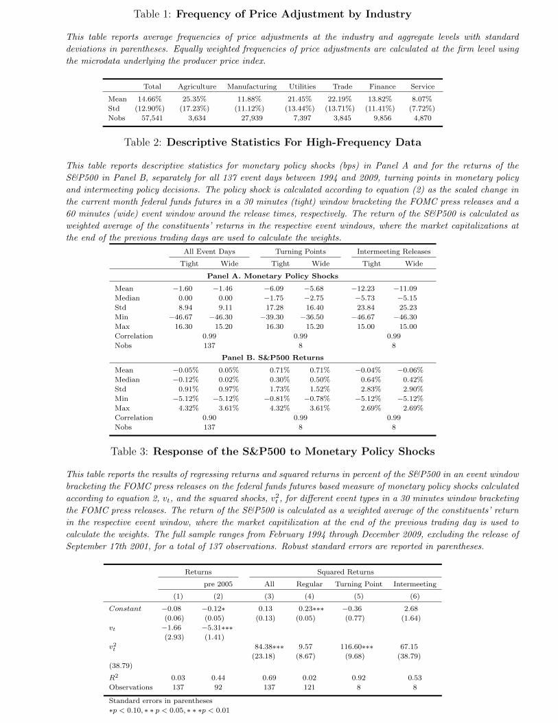
Table 1: Frequency of Price Adjustment by Industry

This table reports average frequencies of price adjustments at the industry and aggregate levels with standard

deviations in parentheses. Equally weighted frequencies of price adjustments are calculated at the firm level using

the microdata underlying the producer price index.

Total Agriculture Manufacturing Utilities Trade Finance Service

Mean 14.66% 25.35% 11.88% 21.45% 22.19% 13.82% 8.07%

Std (12.90%) (17.23%) (11.12%) (13.44%) (13.71%) (11.41%) (7.72%)

Nobs 57,541 3,634 27,939 7,397 3,845 9,856 4,870

Table 2: Descriptive Statistics For High-Frequency Data

This table reports descriptive statistics for monetary policy shocks (bps) in Panel A and for the returns of the

S&P500 in Panel B, separately for all 137 event days between 1994 and 2009, turning points in monetary policy

and intermeeting policy decisions. The policy shock is calculated according to equation (2) as the scaled change in

the current month federal funds futures in a 30 minutes (tight) window bracketing the FOMC press releases and a

60 minutes (wide) event window around the release times, respectively. The return of the S&P500 is calculated as

weighted average of the constituents’ returns in the respective event windows, where the market capitalizations at

the end of the previous trading days are used to calculate the weights.

All Event Days Turning Points Intermeeting Releases

Tight Wide Tight Wide Tight Wide

Panel A. Monetary Policy Shocks

Mean −1.60 −1.46 −6.09 −5.68 −12.23 −11.09

Median 0.00 0.00 −1.75 −2.75 −5.73 −5.15

Std 8.94 9.11 17.28 16.40 23.84 25.23

Min −46.67 −46.30 −39.30 −36.50 −46.67 −46.30

Max 16.30 15.20 16.30 15.20 15.00 15.00

Correlation 0.99 0.99 0.99

Nobs 137 8 8

Panel B. S&P500 Returns

Mean −0.05% 0.05% 0.71% 0.71% −0.04% −0.06%

Median −0.12% 0.02% 0.30% 0.50% 0.64% 0.42%

Std 0.91% 0.97% 1.73% 1.52% 2.83% 2.90%

Min −5.12% −5.12% −0.81% −0.78% −5.12% −5.12%

Max 4.32% 3.61% 4.32% 3.61% 2.69% 2.69%

Correlation 0.90 0.99 0.99

Nobs 137 8 8

Table 3: Response of the S&P500 to Monetary Policy Shocks

This table reports the results of regressing returns and squared returns in percent of the S&P500 in an event window

bracketing the FOMC press releases on the federal funds futures based measure of monetary policy shocks calculated

according to equation 2, vt, and the squared shocks, v2t , for different event types in a 30 minutes window bracketing

the FOMC press releases. The return of the S&P500 is calculated as a weighted average of the constituents’ return

in the respective event window, where the market capitilization at the end of the previous trading day is used to

calculate the weights. The full sample ranges from February 1994 through December 2009, excluding the release of

September 17th 2001, for a total of 137 observations. Robust standard errors are reported in parentheses.

Returns Squared Returns

pre 2005 All Regular Turning Point Intermeeting

(1) (2) (3) (4) (5) (6)

Constant −0.08 −0.12∗ 0.13 0.23∗∗∗ −0.36 2.68

(0.06) (0.05) (0.13) (0.05) (0.77) (1.64)

vt −1.66 −5.31∗∗∗(2.93) (1.41)

v2t 84.38∗∗∗ 9.57 116.60∗∗∗ 67.15

(23.18) (8.67) (9.68) (38.79)

(38.79)

R2 0.03 0.44 0.69 0.02 0.92 0.53

Observations 137 92 137 121 8 8

Standard errors in parentheses

∗p < 0.10, ∗ ∗ p < 0.05, ∗ ∗ ∗p < 0.01

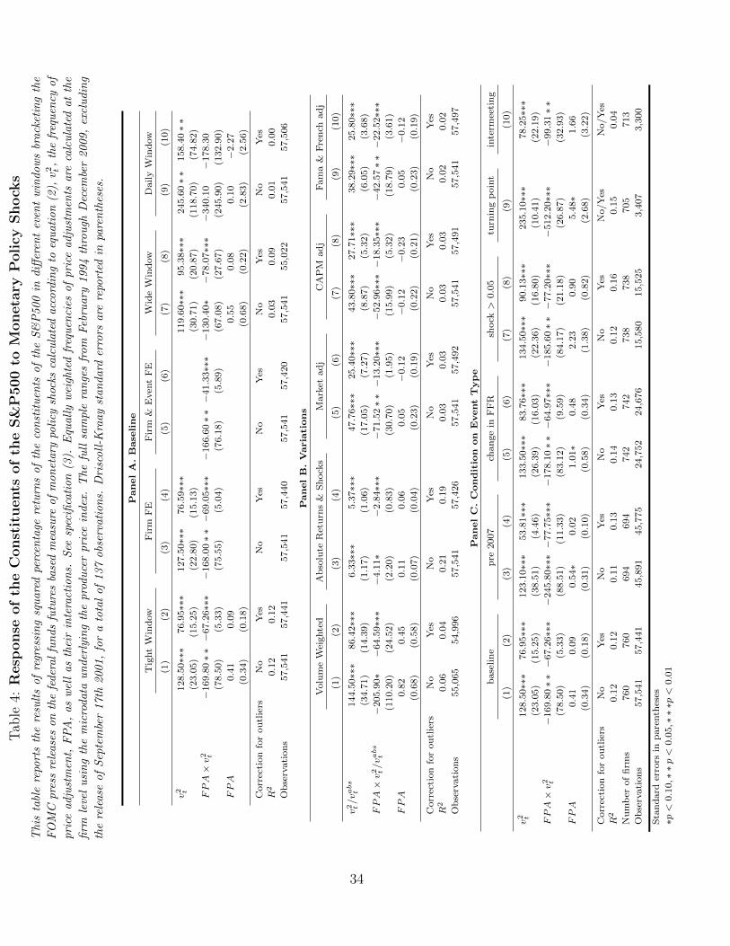
Tab

le4:

Resp

onse

of

the

Const

ituents

of

the

S&

P500

toM

oneta

ryP

oli

cyShock

s

This

tabl

ere

port

sth

ere

sult

sof

regr

essi

ng

squ

are

dpe

rcen

tage

retu

rns

of

the

con

stit

uen

tsof

the

S&

P500

indiff

eren

tev

ent

win

dow

sbr

ack

etin

gth

e

FO

MC

pre

ssre

lease

son

the

feder

al

fun

ds

futu

res

base

dm

easu

reof

mon

etary

poli

cysh

ocks

calc

ula

ted

acc

ord

ing

toeq

uati

on

(2),v2 t,

the

freq

uen

cyof

pri

ceadju

stm

ent,

FP

A,

as

wel

las

thei

rin

tera

ctio

ns.

See

spec

ifica

tion

(3).

Equ

all

yw

eigh

ted

freq

uen

cies

of

pri

ceadju

stm

ents

are

calc

ula

ted

at

the

firm

leve

lu

sin

gth

em

icro

data

un

der

lyin

gth

epro

du

cer

pri

cein

dex

.T

he

full

sam

ple

ran

ges

from

Feb

ruary

1994

thro

ugh

Dec

embe

r2009,

excl

udin

g

the

rele

ase

of

Sep

tem

ber

17th

2001,

for

ato

tal

of

137

obs

erva

tion

s.D

risc

oll

-Kra

ay

stan

dard

erro

rsare

repo

rted

inpa

ren

thes

es.

PanelA.Base

line

Tig

ht

Win

dow

Fir

mF

EF

irm

&E

ven

tF

EW

ide

Win

dow

Daily

Win

dow

(1)

(2)

(3)

(4)

(5)

(6)

(7)

(8)

(9)

(10)

v2 t

128.5

0∗∗∗

76.9

5∗∗∗

127.5

0∗∗∗

76.5

9∗∗∗

119.6

0∗∗∗

95.3

8∗∗∗

245.6

0∗∗

158.4

0∗∗

(23.0

5)

(15.2

5)

(22.8

0)

(15.1

3)

(30.7

1)

(20.8

7)

(118.7

0)

(74.8

2)

FPA×v

2 t−

169.8

0∗∗−

67.2

6∗∗∗

−168.0

0∗∗−

69.0

5∗∗∗

−166.6

0∗∗−

41.3

3∗∗∗

−130.4

0∗

−78.0

7∗∗∗

−340.1

0−

178.3

0

(78.5

0)

(5.3

3)

(75.5

5)

(5.0

4)

(76.1

8)

(5.8

9)

(67.0

8)

(27.6

7)

(245.9

0)

(132.9

0)

FPA

0.4

10.0

90.5

50.0

80.1

0−

2.2

7

(0.3

4)

(0.1

8)

(0.6

8)

(0.2

2)

(2.8

3)

(2.5

6)

Corr

ecti

on

for

ou

tlie

rsN

oY

esN

oY

esN

oY

esN

oY

esN

oY

es

R2

0.1

20.1

20.0

30.0

90.0

10.0

0

Ob

serv

ati

on

s57,5

41

57,4

41

57,5

41

57,4

40

57,5

41

57,4

20

57,5

41

55,0

22

57,5

41

57,5

06

PanelB.Variations

Volu

me

Wei

ghte

dA

bso

lute

Ret

urn

s&

Sh

ock

sM

ark

etad

jC

AP

Mad

jF

am

a&

Fre

nch

ad

j

(1)

(2)

(3)

(4)

(5)

(6)

(7)

(8)

(9)

(10)

v2 t/vabs

t144.5

0∗∗∗

86.4

2∗∗∗

6.3

3∗∗∗

5.3

7∗∗∗

47.7

6∗∗∗

25.4

0∗∗∗

43.8

0∗∗∗

27.7

1∗∗∗

38.2

9∗∗∗

25.8

0∗∗∗

(34.7

1)

(14.3

9)

(1.1

7)

(1.0

6)

(17.0

5)

(7.2

7)

(8.8

7)

(5.3

2)

(6.0

5)

(3.6

8)

FPA×v

2 t/vabs

t−

205.9

0∗

−64.5

9∗∗∗

−4.1

1∗

−2.8

4∗∗∗

−71.5

2∗∗−

13.2

0∗∗∗

−52.9

6∗∗∗−

18.3

5∗∗∗

−42.5

7∗∗−

22.5

2∗∗∗

(110.2

0)

(24.5

2)

(2.2

0)

(0.8

3)

(30.7

0)

(1.9

5)

(15.9

9)

(5.3

2)

(18.7

9)

(3.6

1)

FPA

0.8

20.4

50.1

10.0

60.0

5−

0.1

2−

0.1

2−

0.2

30.0

5−

0.1

2

(0.6

8)

(0.5

8)

(0.0

7)

(0.0

4)

(0.2

3)

(0.1

9)

(0.2

2)

(0.2

1)

(0.2

3)

(0.1

9)

Corr

ecti

on

for

ou

tlie

rsN

oY

esN

oY

esN

oY

esN

oY

esN

oY

es

R2

0.0

60.0

40.2

10.1

90.0

30.0

30.0

30.0

30.0

20.0

2

Ob

serv

ati

on

s55,0

65

54,9

96

57,5

41

57,4

26

57,5

41

57,4

92

57,5

41

57,4

91

57,5

41

57,4

97

PanelC.Condition

on

EventType

base

lin

ep

re2007

chan

ge

inF

FR

shock>

0.0

5tu

rnin

gp

oin

tin

term

eeti

ng

(1)

(2)

(3)

(4)

(5)

(6)

(7)

(8)

(9)

(10)

v2 t

128.5

0∗∗∗

76.9

5∗∗∗

123.1

0∗∗∗

53.8

1∗∗∗

133.5

0∗∗∗

83.7

6∗∗∗

134.5

0∗∗∗

90.1

3∗∗∗

235.1

0∗∗∗

78.2

5∗∗∗

(23.0

5)

(15.2

5)

(38.5

1)

(4.4

6)

(26.3

9)

(16.0

3)

(22.3

6)

(16.8

0)

(10.4

1)

(22.1

9)

FPA×v

2 t−

169.8

0∗∗−

67.2

6∗∗∗

−245.8

0∗∗∗−

77.7

5∗∗∗

−178.1

0∗∗−

64.9

7∗∗∗

−185.6

0∗∗−

77.2

0∗∗∗

−512.2

0∗∗∗

−99.3

1∗∗

(78.5

0)

(5.3

3)

(88.5

1)

(11.3

3)

(83.1

2)

(9.5

9)

(84.1

7)

(21.1

8)

(26.8

7)

(32.9

3)

FPA

0.4

10.0

90.5

4∗

0.0

21.0

1∗

0.4

82.2

30.9

05.4

8∗

1.6

6

(0.3

4)

(0.1

8)

(0.3

1)

(0.1

0)

(0.5

8)

(0.3

4)

(1.3

8)

(0.8

2)

(2.6

8)

(3.2

2)

Corr

ecti

on

for

ou

tlie

rsN

oY

esN

oY

esN

oY

esN

oY

esN

o/Y

esN

o/Y

es

R2

0.1

20.1

20.1

10.1

30.1

40.1

30.1

20.1

60.1

50.0

4

Nu

mb

erof

firm

s760

760

694

694

742

742

738

738

705

713

Ob

serv

ati

on

s57,5

41

57,4

41

45,8

91

45,7

75

24,7

52

24,6

76

15,5

80

15,5

25

3,4

07

3,3

00

Sta

nd

ard

erro

rsin

pare

nth

eses

∗p<

0.1

0,∗∗p<

0.0

5,∗∗∗p<

0.0

1

34

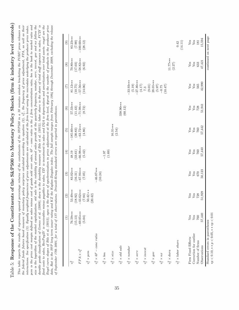
Tab

le5:

Resp

onse

of

the

Const

ituents

of

the

S&

P500

toM

oneta

ryP

oli

cyShock

s(fi

rm&

indust

ryle

vel

contr

ols

)

Th

ista

ble

repo

rts

the

resu

lts

of

regr

essi

ng

squ

are

dpe

rcen

tage

retu

rns

of

the

con

stit

uen

tso

fth

eS

&P

50

0in

a3

0m

inu

tes

win

do

wbr

ack

etin

gth

eF

OM

Cp

ress

rele

ase

so

n

the

fed

era

lfu

nd

sfu

ture

sba

sed

mea

sure

of

mo

net

ary

poli

cysu

rpri

ses

calc

ula

ted

acc

ord

ing

toeq

ua

tio

n(2

),v

2 t,

the

freq

uen

cyo

fp

rice

ad

just

men

t,F

PA

,a

sw

ell

as

thei

r

inte

ract

ion

s.S

eesp

ecifi

cati

on

(3).

Equ

all

yw

eigh

ted

freq

uen

cies

of

pri

cea

dju

stm

ents

are

calc

ula

ted

at

the

firm

leve

lu

sin

gth

em

icro

da

tau

nd

erly

ing

the

pro

du

cer

pri

cein

dex

.

pcm

isth

ep

rice

cost

ma

rgin

defi

ned

as

sale

sm

inu

sco

sto

fgo

ods

sold

ove

rsa

les,

4F−concratio

isth

e4

firm

con

cen

tra

tio

nra

tio

,bm

isth

ebo

ok

tom

ark

etra

tio

an

d

size

isth

elo

gari

thm

of

the

ma

rket

cap

ita

liza

tio

n.stdsale

isth

evo

lati

lity

of

an

nu

al

sale

sgr

ow

tha

tth

equ

art

erly

freq

uen

cy,nondur,serv

,invest,gov

an

dnx

foll

ow

the

du

rabl

ego

ods

cla

ssifi

cati

on

of

Go

mes

eta

l.(2

00

9),dura

isth

ed

ura

bili

tym

easu

reo

fB

ils

eta

l.(2

01

2),laborshare

isth

esh

are

of

tota

lst

aff

expe

nse

sin

sale

s,FC

2Y

is

fixe

dco

sts

tosa

les,RecPay2Y

isre

ceiv

abl

esm

inu

spa

ya

bles

tosa

les,I2Y

isin

vest

men

tto

sale

sa

ndD

2A

isd

epre

cia

tio

na

nd

am

ort

iza

tio

no

ver

tota

la

sset

s.engel

are

the

En

gel

curv

esl

ope

so

fB

ils

eta

l.(2

01

2),sync

isth

ed

egre

eo

fsy

nch

ron

iza

tio

nin

pri

cea

dju

stm

ent

at

the

firm

leve

l,#prod

isth

en

um

ber

of

pro

du

cts

inth

ep

rod

uce

rp

rice

da

ta,Rat

isth

eS

&P

lon

gte

rmis

suer

rati

ng

an

dKZ

the

Ka

pla

n-Z

inga

les

ind

ex.

Th

efu

llsa

mp

lera

nge

sfr

om

Feb

rua

ry1

99

4th

rou

ghD

ecem

ber

20

09

,ex

clu

din

gth

ere

lea

se

of

Sep

tem

ber

17

th2

00

1,

for

ato

tal

of

13

7o

bser

vati

on

s.D

risc

oll

-Kra

ay

sta

nd

ard

erro

rsa

rere

port

edin

pare

nth

eses

.

(1)

(2)

(3)

(4)

(5)

(6)

(7)

(8)

(9)

v2 t

76.5

9∗∗∗

53.4

9∗∗∗

83.0

2∗∗∗

48.1

9−

185.6

0∗∗∗

57.3

3∗∗∗

81.1

2∗∗∗

70.8

0∗∗∗

83.2

3∗∗∗

(15.1

3)

(18.9

2)

(16.3

1)

(33.6

1)

(30.8

3)

(11.4

3)

(10.7

5)

(17.0

3)

(7.9

0)

FPA×v

2 t−

69.0

5∗∗∗

−43.6

2∗∗∗

−67.9

4∗∗∗

−66.9

8∗∗∗

−63.7

2∗∗∗

−71.9

8∗∗∗

−57.5

6∗∗∗

−58.8

2∗∗∗

−100.6

0∗∗∗

(5.0

4)

(7.8

4)

(7.0

5)

(5.4

2)

(4.8

6)

(8.7

2)

(14.0

6)

(6.9

2)

(28.1

2)

v2 t×pcm

50.4

2∗∗

(20.4

2)

v2 t×

4F−concratio

−46.8

7∗∗∗

(10.2

4)

v2 t×bm

−1.9

7

(1.6

9)

v2 t×size

16.3

1∗∗∗

(2.5

4)

v2 t×stdsale

338.9

0∗∗∗

(60.1

2)

v2 t×nondur

−33.9

3∗∗∗

(5.1

9)

v2 t×serv

−27.4

6∗∗∗

(4.1

7)

v2 t×invest

7.3

(9.0

1)

v2 t×gov

28.0

1∗∗∗

(5.9

7)

v2 t×nx

−0.7

5

(10.4

7)

v2 t×dura

11.7

7∗∗∗

(2.2

7)

v2 t×laborshare

0.4

2

(14.1

1)

Fir

mF

ixed

Eff

ects

Yes

Yes

Yes

Yes

Yes

Yes

Yes

Yes

Yes

Corr

ecti

on

for

ou

tlie

rY

esY

esY

esY

esY

esY

esY

esY

esY

es

Nu

mb

erof

firm

s760

728

670

760

760

728

565

633

181

Ob

serv

ati

on

s57,4

40

51,9

29

50,1

23

57,4

40

57,4

42

51,9

41

42,9

90

47,4

21

15,5

94

Sta

nd

ard

erro

rsin

pare

nth

eses

conti

nu

edon

nex

tp

age

∗p<

0.1

0,∗∗p<

0.0

5,∗∗∗p<

0.0

1

35

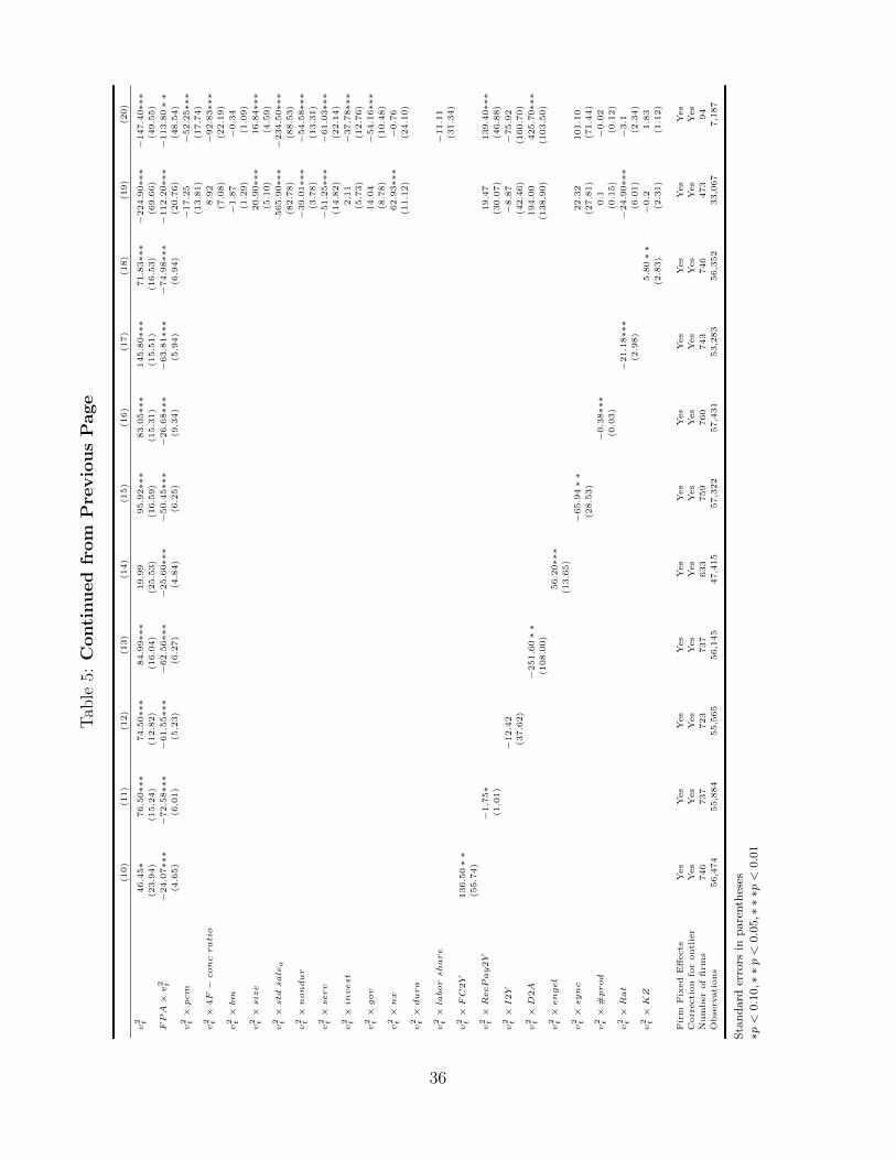
Tab

le5:

Conti

nued

from

Pre

vio

us

Page

(10)

(11)

(12)

(13)

(14)

(15)

(16)

(17)

(18)

(19)

(20)

v2 t

46.4

5∗

76.5

0∗∗

∗74.5

0∗∗

∗84.9

9∗∗

∗19.9

995.9

2∗∗

∗83.0

5∗∗

∗145.8

0∗∗

∗71.8

3∗∗

∗−

224.9

0∗∗

∗−

147.4

0∗∗

∗(2

3.9

4)

(15.2

4)

(12.8

2)

(16.0

4)

(25.5

3)

(16.5

9)

(15.3

1)

(15.5

1)

(16.5

3)

(69.6

6)

(49.5

5)

FPA

×v2 t

−24.0

7∗∗

∗−

72.5

8∗∗

∗−

61.5

5∗∗

∗−

62.5

6∗∗

∗−

25.6

0∗∗

∗−

50.4

5∗∗

∗−

26.6

8∗∗

∗−

63.8

1∗∗

∗−

74.9

8∗∗

∗−

112.2

0∗∗

∗−

113.8

0∗∗

(4.6

5)

(6.0

1)

(5.2

3)

(6.2

7)

(4.8

4)

(6.2

5)

(9.3

4)

(5.9

4)

(6.9

4)

(20.7

6)

(48.5

4)

v2 t×

pcm

−17.2

5−

52.2

5∗∗

∗(1

3.8

1)

(17.7

4)

v2 t×

4F

−concratio

8.9

2−

92.8

3∗∗

∗(7

.08)

(22.1

9)

v2 t×

bm

−1.8

7−

0.3

4

(1.2

9)

(1.0

9)

v2 t×

siz

e20.9

0∗∗

∗16.8

4∗∗

∗(5

.10)

(4.5

9)

v2 t×

std

sale

a565.9

0∗∗

∗−

234.5

0∗∗

∗(8

2.7

8)

(88.5

3)

v2 t×

nondur

−39.0

1∗∗

∗−

54.5

8∗∗

∗(3

.78)

(13.3

1)

v2 t×

serv

−51.2

5∗∗

∗−

61.0

3∗∗

∗(1

4.8

2)

(22.1

4)

v2 t×

invest

2.1

1−

37.7

8∗∗

∗(5

.73)

(12.7

6)

v2 t×

gov

14.0

4−

54.1

6∗∗

∗(8

.78)

(10.4

8)

v2 t×

nx

62.9

3∗∗

∗−

0.7

6

(11.1

2)

(24.1

0)

v2 t×

dura

v2 t×

labor

share

−11.1

1

(31.3

4)

v2 t×

FC

2Y

136.5

0∗∗

(55.7

4)

v2 t×

RecPay2Y

−1.7

5∗

19.4

7139.4

0∗∗

∗(1

.01)

(30.0

7)

(46.8

8)

v2 t×

I2Y

−12.4

2−

8.8

7−

75.9

2

(37.6

2)

(42.4

6)

(160.7

0)

v2 t×

D2A

−251.6

0∗∗

194.0

0425.7

0∗∗

∗(1

08.0

0)

(138.9

0)

(103.5

0)

v2 t×

engel

56.2

0∗∗

∗(1

3.6

5)

v2 t×

sync

−65.9

4∗∗

22.3

2101.1

0

(28.5

3)

(27.8

1)

(71.4

4)

v2 t×

#prod

−0.3

8∗∗

∗0.1

−0.0

2

(0.0

3)

(0.1

5)

(0.1

2)

v2 t×

Rat

−21.1

8∗∗

∗−

24.9

0∗∗

∗−

3.1

(2.9

8)

(6.0

1)

(2.3

4)

v2 t×

KZ

5.8

0∗∗

−0.2

1.8

3

(2.8

3)

(2.3

1)

(1.1

2)

Fir

mF

ixed

Eff

ects

Yes

Yes

Yes

Yes

Yes

Yes

Yes

Yes

Yes

Yes

Yes

Corr

ecti

on

for

outl

ier

Yes

Yes

Yes

Yes

Yes

Yes

Yes

Yes

Yes

Yes

Yes

Num

ber

of

firm

s746

737

723

737

633

759

760

743

746

473

94

Obse

rvati

ons

56,4

74

55,8

84

55,5

65

56,1

45

47,4

15

57,3

22

57,4

31

53,2

83

56,3

52

33,0

67

7,1

87

Sta

nd

ard

erro

rsin

pare

nth

eses

∗p<

0.1

0,∗∗p<

0.0

5,∗∗∗p<

0.0

1

36

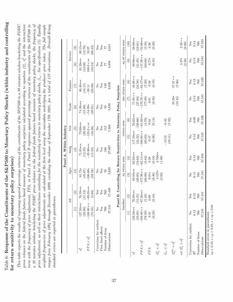
Tab

le6:

Resp

onse

of

the

Con

stit

uents

of

the

S&

P500

toM

oneta

ryP

oli

cyShock

s(w

ithin

indust

ryand

contr

oll

ing

for

retu

rnse

nsi

tivit

yto

moneta

ryp

oli

cysu

rpri

ses)

This

tabl

ere

port

sth

ere

sult

sof

regr

essi

ng

squ

are

dpe

rcen

tage

retu

rns

of

the

con

stit

uen

tsof

the

S&

P500

ina

30

min

ute

sw

indow

brack

etin

gth

eF

OM

C

pre

ssre

lease

son

the

feder

al

fun

ds

futu

res

base

dm

easu

reof

mon

etary

poli

cysu

rpri

ses

calc

ula

ted

acc

ord

ing

toeq

uati

on

(2),v2 t

an

dth

ein

tera

ctio

n

term

wit

hth

efr

equ

ency

of

pri

ceadju

stm

ent,

FP

A,

inP

an

elA

.P

an

elB

regr

esse

ssq

uare

dpe

rcen

tage

retu

rns

of

the

con

stit

uen

tsof

the

S&

P500

in

a30

min

ute

sw

indow

brack

etin

gth

eF

OM

Cpre

ssre

lease

son

the

feder

al

fun

ds

futu

res

base

dm

easu

reof

mon

eta

rypo

licy

shoc

ks,

the

freq

uen

cyof

pri

ceadju

stm

ent,

as

wel

las

thei

rin

tera

ctio

ns

con

troll

ing

for

the

sen

siti

vity

of

retu

rns

tom

on

etary

poli

cysh

ocks

,βvt.

See

spec

ifica

tion

(3).

Equ

all

y

wei

ghte

dfr

equ

enci

esof

pri

ceadju

stm

ents

are

calc

ula

ted

at

the

firm

leve

lu

sin

gth

em

icro

data

un

der

lyin

gth

epro

du

cer

pri

cein

dex

.T

he

full

sam

ple

ran

ges

from

Feb

ruary

1994

thro

ugh

Dec

embe

r2009,

excl

udin

gth

ere

lease

of

Sep

tem

ber

17th

2001,

for

ato

tal

of

137

obs

erva

tion

s.D

risc

oll

-Kra

ay

stan

dard

erro

rsare

repo

rted

inpa

ren

thes

es.

PanelA.W

ithin

Industry

All

Agro

Mn

fgU

til

Tra

de

Fin

an

ceS

ervic

e

(1)

(2)

(3)

(4)

(5)

(6)

(7)

(8)

(9)

v2 t

127.5

0∗∗∗

76.5

9∗∗∗

81.7

3∗

71.8

5∗∗∗

73.6

8∗∗∗

74.3

8∗∗∗

86.4

8∗∗∗

61.2

8∗∗∗

80.1

5∗∗∗

(22.8

0)

(15.1

3)

(45.8

7)

(12.3

3)

(20.5

9)

(15.9

9)

(19.1

5)

(13.0

8)

(13.7

8)

FPA×v

2 t−

168.0

0∗∗−

69.0

5∗∗∗

−106.6

0∗

−35.9

8∗∗∗

−125.0∗∗∗

−54.9

9∗

−20.1

1168.6∗∗∗

33.9

7

(75.5

5)

(5.0

4)

(58.5

8)

(11.5

5)

(16.2

8)

(29.9

1)

(24.9

8)

(53.5

4)

(69.2

3)

Corr

ecti

on

for

ou

tlie

rsN

oY

esN

oN

oN

oN

oN

oN

oY

es

Fir

mfi

xed

effec

tsY

esY

esY

esY

esY

esY

esY

esY

esY

es

Nu

mb

erof

firm

s760

760

58

346

112

50

140

77

77

Ob

serv

ati

on

s57,5

41

57,4

40

3,6

29

27,8

87

7,3

94

3,8

39

9,8

36

4,8

56

4,8

15

PanelB.Controllin

gforRetu

rn

Sensitivitiesto

Moneta

ry

Policy

Surprises

base

lin

esq

retu

rnse

ns

retu

rnse

ns

ab

sre

turn

sen

ssq

rel

retu

rnse

ns

(1)

(2)

(3)

(4)

(5)

(6)

(7)

(8)

(9)

(10)

v2 t

128.5

0∗∗∗

76.9

5∗∗∗

93.8

3∗∗∗

62.0

3∗∗∗

117.1

0∗∗∗

70.6

3∗∗∗

71.9

5∗∗

49.8

9∗∗

89.9

8∗∗∗

58.0

8∗∗∗

(23.0

5)

(15.2

5)

(20.0

5)

(19.6

2)

(24.3

2)

(20.6

6)

(27.9

3)

(24.5

8)

(21.0

5)

(19.6

1)

FPA×v

2 t−

169.8

0∗∗−

67.2

6∗∗∗

−157.9

0∗∗−

62.1

1∗∗∗

−160.8

0∗∗−

61.0

2∗∗∗

−170.7

0∗∗−

62.1

7∗∗∗

−147.3

0∗∗−

52.8

6∗∗∗

(78.5

0)

(5.3

3)

(68.8

9)

(8.6

4)

(65.6

3)

(4.7

0)

(77.8

9)

(7.2

9)

(63.6

8)

(5.5

8)

FPA

0.4

10.0

90.8

1∗

0.2

80.4

70.0

10.6

10.1

60.7

7∗

0.2

6

(0.3

4)

(0.1

8)

(0.4

6)

(0.1

9)

(0.3

8)

(0.1

4)

(0.3

9)

(0.1

9)

(0.4

5)

(0.2

0)

β2 vt×v

2 t5.5

37∗

2.7

06∗∗

(2.9

3)

(1.0

9)

βvt×v

2 t−

13.5

2−

6.4

2

(19.1

1)

(7.9

2)

βabs

vt×v

2 t35.2

0∗

17.2

1∗∗

(19.4

3)

(7.9

0)

relβ

2 vt×v

2 t4.3

7∗

2.3

0∗∗

(2.3

8)

(0.9

9)

Corr

ecti

on

for

ou

tlie

rsN

oY

esN

oY

esN

oY

esN

oY

esN

oY

es

R2

0.1

20.1

20.1

50.1

40.1

20.0

90.1

40.1

30.1

40.1

4

Nu

mb

erof

firm

s760

760

760

760

760

760

760

760

760

760

Ob

serv

ati

on

s57,5

41

57,4

41

57,5

41

57,4

33

57,5

41

57,4

36

57,5

41

57,4

29

57,5

41

57,4

33

Sta

nd

ard

erro

rsin

pare

nth

eses

∗p<

0.1

0,∗∗p<

0.0

5,∗∗∗p<

0.0

1

37

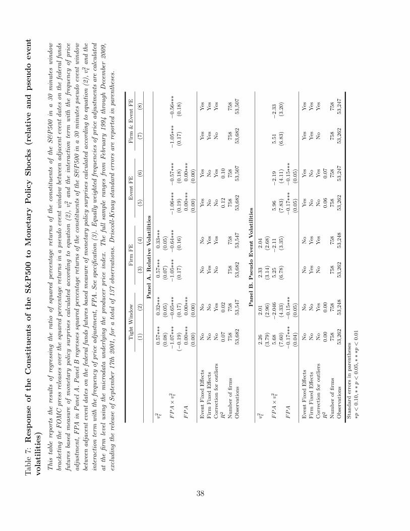
Tab

le7:

Resp

onse

of

the

Const

ituents

of

the

S&

P500

toM

oneta

ryP

oli

cyShock

s(r

ela

tive

and

pse

udo

event

vola

tiliti

es)

This

tabl

ere

port

sth

ere

sult

sof

regr

essi

ng

the

rati

oof

squ

are

dpe

rcen

tage

retu

rns

of

the

con

stit

uen

tsof

the

S&

P500

ina

30

min

ute

sw

indow

brack

etin

gth

eF

OM

Cpre

ssre

lease

sove

rth

esq

uare

dpe

rcen

tage

retu

rns

ina

pse

udo

even

tw

indow

betw

een

adja

cen

tev

ent

da

tes

on

the

feder

al

fun

ds

futu

res

base

dm

easu

reof

mon

etary

poli

cysu

rpri

ses

calc

ula

ted

acc

ord

ing

toeq

uati

on

(2),v2 t

an

dth

ein

tera

ctio

nte

rmw

ith

the

freq

uen

cyof

pri

ce

adju

stm

ent,

FP

Ain

Pan

elA

.P

an

elB

regr

esse

ssq

uare

dpe

rcen

tage

retu

rns

of

the

con

stit

uen

tsof

the

S&

P500

ina

30

min

ute

spse

udo

even

tw

indo

w

betw

een

adja

cen

tev

ent

date

son

the

feder

al

fun

ds

futu

res

base

dm

easu

reof

mon

etary

poli

cysu

rpri

ses

calc

ula

ted

acc

ord

ing

toeq

uati

on

(2),v2 t

an

dth

e

inte

ract

ion

term

wit

hth

efr

equ

ency

of

pri

ceadju

stm

ent,

FP

A.

See

spec

ifica

tion

(3).

Equ

all

yw

eigh

ted

freq

uen

cies

of

pri

ceadju

stm

ents

are

calc

ula

ted

at

the

firm

leve

lu

sin

gth

em

icro

data

un

der

lyin

gth

epro

du

cer

pri

cein

dex

.T

he

full

sam

ple

ran

ges

from

Feb

ruary

1994

thro

ugh

Dec

embe

r2009,

excl

udin

gth

ere

lease

of

Sep

tem

ber

17th

2001,

for

ato

tal

of

137

obs

erva

tion

s.D

risc

oll

-Kra

ay

stan

dard

erro

rsare

repo

rted

inpa

ren

thes

es.

Tig

ht

Win

dow

Fir

mF

EE

ven

tF

EF

irm

&E

ven

tF

E

(1)

(2)

(3)

(4)

(5)

(6)

(7)

(8)

PanelA.RelativeVolatilities

v2 t

0.5

7∗∗∗

0.3

2∗∗∗

0.5

7∗∗∗

0.3

3∗∗∗

(0.0

8)

(0.0

5)

(0.0

7)

(0.0

5)

FPA×v

2 t−

1.0

7∗∗∗−

0.6

5∗∗∗

−1.0

5∗∗∗−

0.6

4∗∗∗

−1.0

6∗∗∗−

0.5

7∗∗∗

−1.0

5∗∗∗−

0.5

6∗∗∗

(−0.1

9)

(0.1

7)

(0.1

7)

(0.1

6)

(0.1

9)

(0.1

8)

(0.1

7)

(0.1

8)

FPA

0.0

0∗∗∗

0.0

0∗∗∗

0.0

0∗∗∗

0.0

0∗∗∗

(0.0

0)

(0.0

0)

(0.0

0)

(0.0

0)

Even

tF

ixed

Eff

ects

No

No

No

No

Yes

Yes

Yes

Yes

Fir

mF

ixed

Eff

ects

No

No

Yes

Yes

No

No

Yes

Yes

Corr

ecti

on

for

ou

tlie

rsN

oY

esN

oY

esN

oY

esN

oY

es

R2

0.0

70.0

20.1

20.1

0

Nu

mb

erof

firm

s758

758

758

758

758

758

758

758

Ob

serv

ati

on

s53,6

82

53,5

47

53,6

82

53,5

47

53,6

82

53,5

07

53,6

82

53,5

07

PanelB.Pse

udo

EventVolatilities

v2 t

2.2

62.0

12.3

32.0

4

(3.7

9)

(2.9

6)

(3.1

4)

(2.6

8)

FPA×v

2 t5.6

8−

2.0

46

5.2

5−

2.1

15.9

6−

2.1

95.5

1−

2.3

3

(7.6

0)

(4.3

3)

(6.7

8)

(3.3

5)

(7.8

3)

(4.1

1)

(6.8

3)

(3.2

0)

FPA

−0.1

7∗∗∗−

0.1

5∗∗∗

−0.1

7∗∗∗−

0.1

5∗∗∗

(0.0

4)

(0.0

5)

(0.0

5)

(0.0

5)

Even

tF

ixed

Eff

ects

No

No

No

No

Yes

Yes

Yes

Yes

Fir

mF

ixed

Eff

ects

No

No

Yes

Yes

No

No

Yes

Yes

Corr

ecti

on

for

ou

tlie

rsN

oY

esN

oY

esN

oY

esN

oY

es

R2

0.0

00.0

00.0

60.0

7

Nu

mb

erof

firm

s758

758

758

758

758

758

758

758

Ob

serv

ati

on

s53,2

62

53,2

48

53,2

62

53,2

48

53,2

62

53,2

47

53,2

62

53,2

47

Sta

nd

ard

erro

rsin

pare

nth

eses

∗p<

0.1

0,∗∗p<

0.0

5,∗∗∗p<

0.0

1

38

Tab

le8:

Resp

onse

of

the

Const

ituents

of

the

S&

P500

toM

oneta

ryP

oli

cyShock

s(p

rofita

bil

ity)

This

tabl

ere

port

sth

ere

sult

sof

regr

essi

ng

squ

are

dpe

rcen

tage

chan

ges

inm

ean

quart

erly

ope

rati

ng

inco

me

befo

redep

reci

ati

on

betw

een

quart

erst+

H

tillt+

H+

3an

dt−

4ti

llt−

1n

orm

ali

zed

byt−

1to

tal

ass

ets

of

the

con

stit

uen

tsof

the

S&

P500

ina

30

min

ute

sw

indow

brack

etin

gth

eF

OM

Cpre

ss

rele

ase

son

the

feder

al

fun

ds

futu

res

base

dm

easu

reof

mon

etary

poli

cysu

rpri

ses

calc

ula

ted

acc

ord

ing

toeq

uati

on

(2)

an

dacc

um

ula

ted

toqu

art

erly

freq

uen

cy,v2 t,

the

freq

uen

cyof

pri

ceadju

stm

ent,

FP

A,

as

wel

las

thei

rin

tera

ctio

n.

See

spec

ifica

tion

(5).

Equ

all

yw

eigh

ted

freq

uen

cies

of

pri

ce

adju

stm

ents

are

calc

ula

ted

at

the

esta

blis

hm

ent

leve

lu

sin

gth

em

icro

data

un

der

lyin

gth

epro

du

cer

pri

cein

dex

.T

he

full

sam

ple

ran

ges

from

Feb

ruary

1994

thro

ugh

Dec

embe

r2009,

excl

udin

gth

ere

lease

of

Sep

tem

ber

17th

2001,

for

ato

tal

of

137

obs

erva

tion

s.D

risc

oll

-Kra

ay

stan

dard

erro

rsare

repo

rted

inpa

ren

thes

es.

H=

0H

=1

H=

2H

=3

H=

4H

=5

H=

6H

=7

H=

8

v2 t

2.4

7∗

1.7

5−

0.0

3−

2.1

0−

3.6

9−

7.9

8∗∗

−10.5

1∗

−15.9

9∗∗∗

−21.5

5∗∗∗

(1.3

5)

(1.6

6)

(1.8

1)

(2.0

4)

(2.9

0)

(3.6

1)

(5.4

6)

(5.8

9)

(7.0

0)

FPA×v

2 t−

19.6

8∗∗∗

−23.9

8∗∗∗

−25.6

2∗∗∗

−30.9

1∗∗

−36.8

1∗∗

−35.1

8∗∗

−41.5

8∗∗

−29.9

8−

29.6

8

(5.2

4)

(7.4

2)

(9.0

6)

(11.8

7)

(15.1

7)

(15.3

9)

(19.5

0)

(20.2

3)

(22.8

5)

FPA

2.1

0∗∗∗

2.6

8∗∗∗

3.2

4∗∗∗

3.7

8∗∗∗

4.0

7∗∗∗

4.0

1∗∗

4.7

7∗∗

4.7

0∗

4.8

8

(0.3

9)

(0.5

9)

(0.8

6)

(1.1

6)

(1.4

3)

(1.7

0)

(2.2

4)

(2.7

0)

(3.3

4)

Corr

ecti

on

for

ou

tlie

rY

esY

esY

esY

esY

esY

esY

esY

esY

es

R2

0.0

10.0

00.0

00.0

00.0

00.0

00.0

00.0

00.0

0

Nu

mb

erof

firm

s685

682

678

671

668

661

660

653

642

Ob

serv

ati

on

s20,7

56

20,4

28

20,1

17

19,8

14

19,6

46

19,4

49

19,2

95

18,9

21

18,4

75

Sta

nd

ard

erro

rsin

pare

nth

eses

∗p<

0.1

0,∗∗p<

0.0

5,∗∗∗p<

0.0

1

39

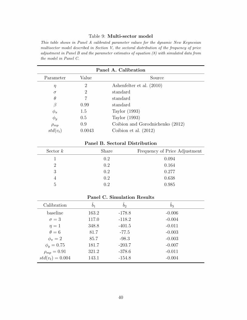
Table 9: Multi-sector modelThis table shows in Panel A calibrated parameter values for the dynamic New Keynesian

multisector model described in Section V, the sectoral distribution of the frequency of price

adjustment in Panel B and the parameter estimates of equation (8) with simulated data from

the model in Panel C.

Panel A. Calibration

Parameter Value Source

η 2 Ashenfelter et al. (2010)

σ 2 standard

θ 7 standard

β 0.99 standard

φπ 1.5 Taylor (1993)

φy 0.5 Taylor (1993)

ρmp 0.9 Coibion and Gorodnichenko (2012)

std(vt) 0.0043 Coibion et al. (2012)

Panel B. Sectoral Distribution

Sector k Share Frequency of Price Adjustment

1 0.2 0.094

2 0.2 0.164

3 0.2 0.277

4 0.2 0.638

5 0.2 0.985

Panel C. Simulation Results

Calibration b1 b2 b3

baseline 163.2 -178.8 -0.006

σ = 3 117.0 -118.2 -0.004

η = 1 348.8 -401.5 -0.011

θ = 6 81.7 -77.5 -0.003

φπ = 2 85.7 -98.3 -0.003

φy = 0.75 181.7 -203.7 -0.007

ρmp = 0.91 321.2 -378.6 -0.011

std(vt) = 0.004 143.1 -154.8 -0.004

40