Are old-growth forests special? Or just old?

How would you know?

Hemlock-northern hardwood forests

Shade-tolerant canopy species:Acer saccharum (sugar maple)Fagus grandifolia (American beech)Tsuga canadensis (eastern hemlock)

Less tolerant canopy species:Betula alleghaniensis (yellow birch)Acer rubrum (red maple)

Shade-tolerant sub-canopy species:Abies balsamea (balsam fir)Ostrya virginiana (hop-hornbeam)

Shade-tolerant canopy, swamp forestThuja occidentalisPicea glauca

Less tolerant canopy, swamp forestFraxinus nigra

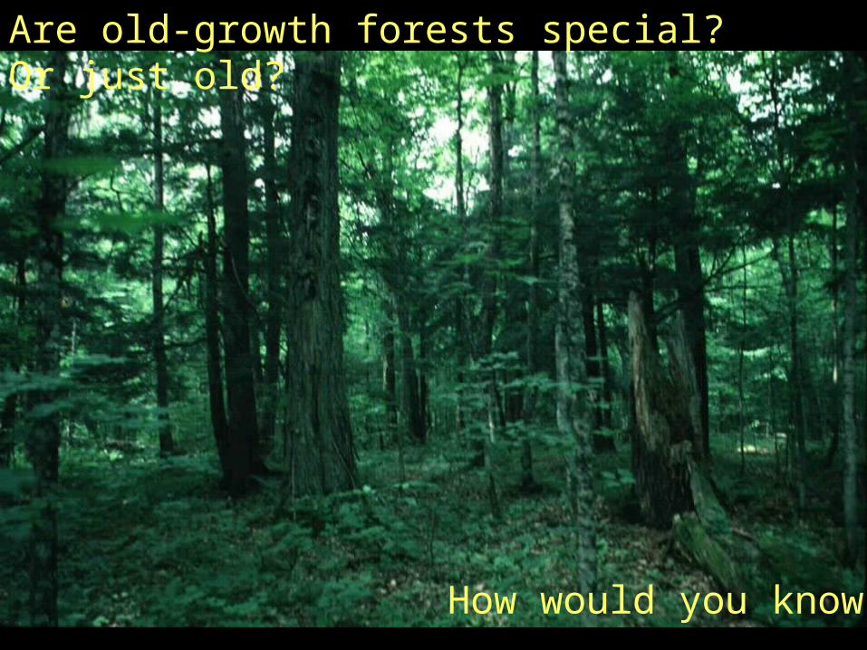
Textbook: Stands at equilibrium composition - frequent, gap-phase -> statistical self-replacement of shade-tolerant dominants - some ‘gap specialists’ persist (Betula alleghaniensis)

Dscn9985.jpg

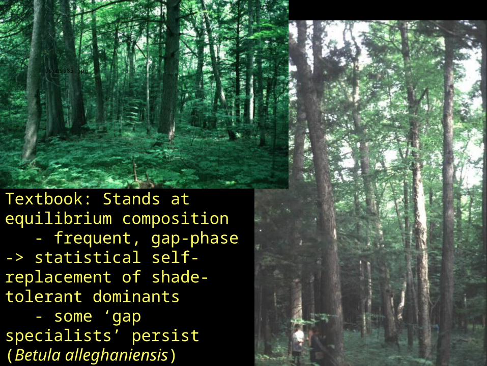
Mesic forests in Upper Great Lakes good candidates for equilibrium: - fire extremely rare - stand-initiating wind-disturbance return time est >2000 yr - large areas with no anthropogenic disturbance

HOWEVER, model rarely tested by direct evidence.

Indirect approaches -- palynology, simulation models, chronosequences -- all have severe limitations in regard to assumptions or scale.

But direct, observational data are difficult to get because SLOW systems.

Dominants can live over 400 years, remain suppressed in understory many decades.

This can be discouraging -- UNLESS...

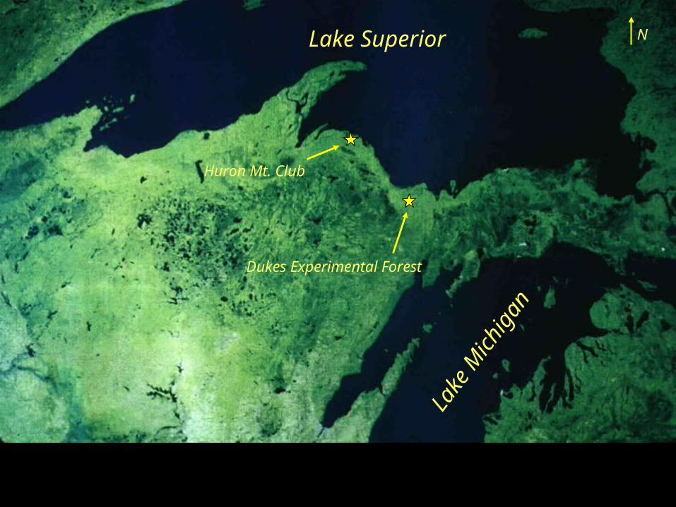
Lake Superior

Lake

Mic

higa

n

Huron Mt. Club

Dukes Experimental Forest

N

200 m

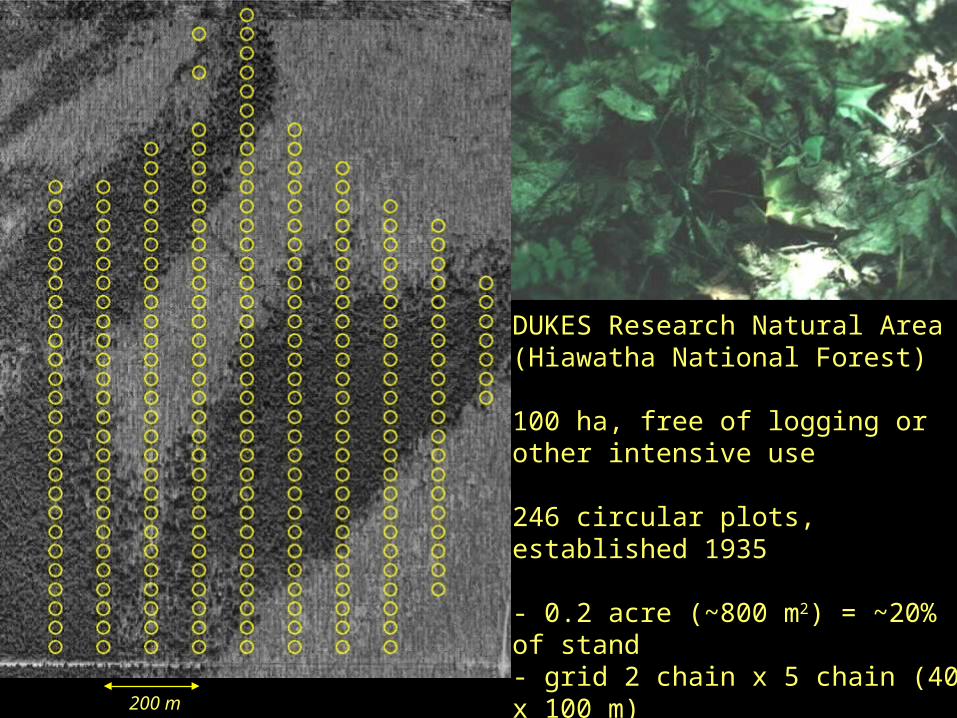
DUKES Research Natural Area(Hiawatha National Forest)

100 ha, free of logging or other intensive use

246 circular plots, established 1935

- 0.2 acre (~800 m2) = ~20% of stand- grid 2 chain x 5 chain (40 x 100 m)

200 m

High Ca,Acer

High Ca,Acer

Peat,conifers

Peat,conifers Hardpan,

mixed

Hardpan,mixed

podzol,Tsuga

podzol,Tsuga

Habitat is spatially patchy

y vs x

East

No

rth

200 m

2D Graph 2

X Data

0 10 20 30 40 50

Y D

ata

0

5

10

15

20

25

30

'4485 vs '4486

2D Graph 1

X Data

0 10 20 30 40 50

Y D

ata

0

5

10

15

20

25

30

Acer saccharumFagus grandifoliaBetula alleghaniensisTsuga canadensisAcer rubrumOther species

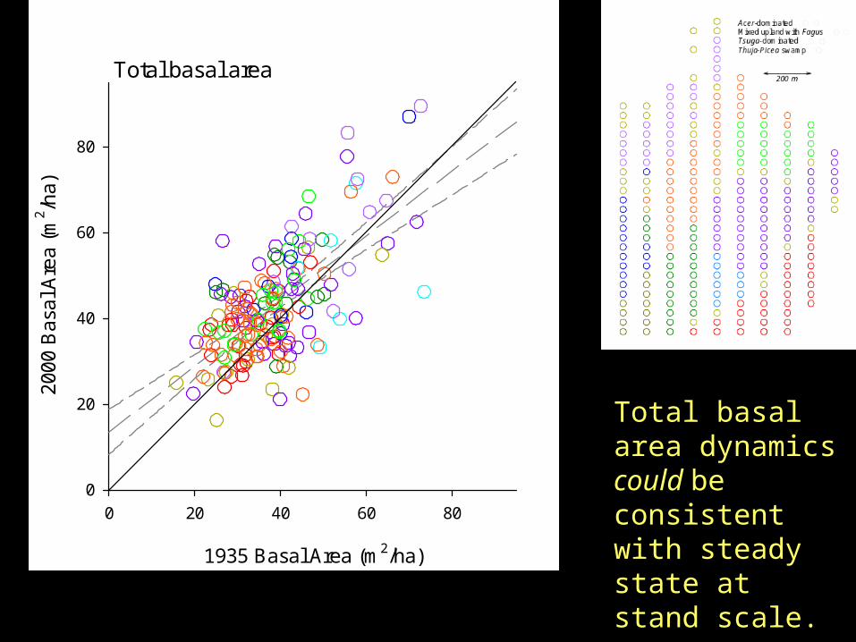
Symbol area scaled to total basal area; maximum basal area = 86.3 m2/ha

20 m

Data set is spatially complicated

1935 1948 1974-1980 1989-2004

n = 238 (8 ‘transitional’plots unsampled)

Stems > 5 in (12.7 cm)dbh tallied by 2.5 cm category

n = 123 (alternating along N-S lines)

Stems > 5 in (12.7 cm)dbh tallied by 2.5 cm category

n = 242

Stems > 0.5 in (1.3 cm)dbh tallied by 0.1 in category

n = 197

Upland: stems > 5 cmmapped full plot, >1 cm8 m radius subplot, remeasured 5-yr cycle.

Swamp: stems >5 cm full plot, >1 cm 8 m sub-plot tallied only

And temporally even more complicated

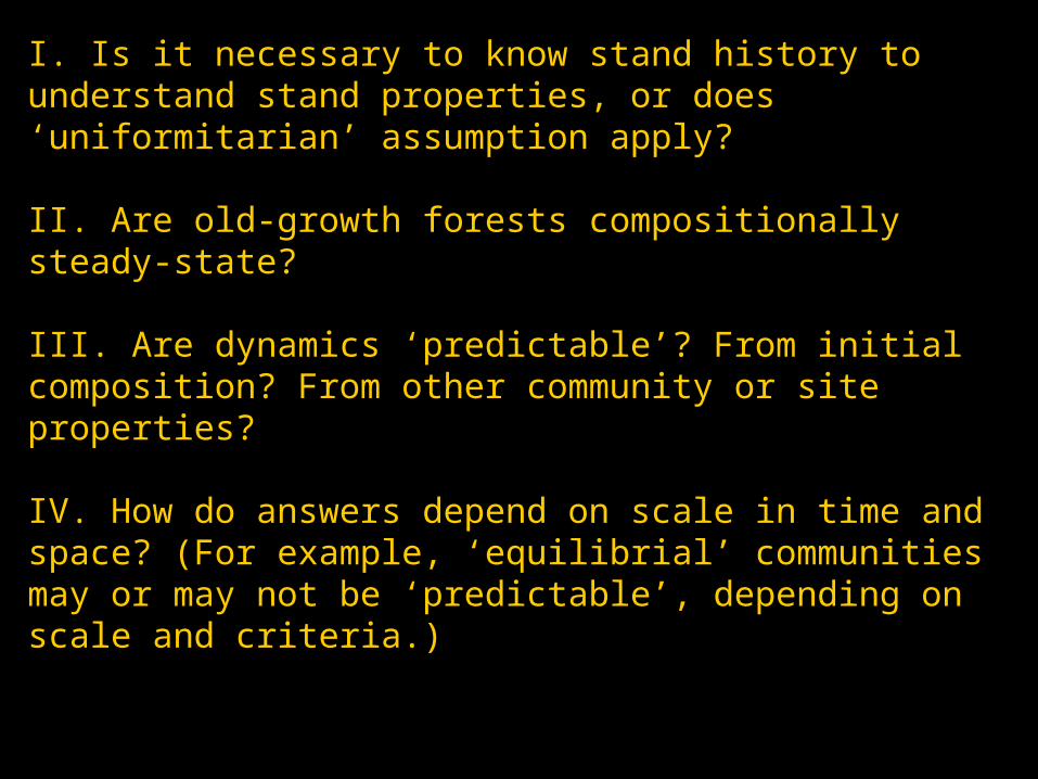
I. Is it necessary to know stand history to understand stand properties, or does ‘uniformitarian’ assumption apply?

II. Are old-growth forests compositionally steady-state?

III. Are dynamics ‘predictable’? From initial composition? From other community or site properties?

IV. How do answers depend on scale in time and space? (For example, ‘equilibrial’ communities may or may not be ‘predictable’, depending on scale and criteria.)

1935 Basal Area (m2/ha)

0 20 40 60 80

20

00

Ba

sal A

rea

(m

2 /ha

)

0

20

40

60

80

Total basal area

Total basal area dynamics could be consistent with steady state at stand scale.

0 10 20 30 40 50

20

00

Ba

sal A

rea

(m

2/h

a)

0

10

20

30

40

50

Acer saccharum

0 10 20 30 40 50 60

0

10

20

30

40

50

60

Tsuga canadensis

1935 Basal Area (m2/ha)

0 2 4 6 8 10 12 14 16 18

20

00

Ba

sal A

rea

(m

2/h

a)

0

2

4

6

8

10

12

14

16

18Fagus grandifolia

1935 Basal Area (m2/ha)

0 20 40 60 80

0

20

40

60

80Thuja occidentalis

Shade-tolerant species are increasing.

But population trends say otherwise

0 5 10 15 20 25 30

20

00

Ba

sal A

rea

(m

2/h

a)

0

5

10

15

20

25

30Betula alleghaniensis

0 2 4 6 8 10

0

2

4

6

8

10Abies balsamea

1935 Basal Area (m2/ha)

0 5 10 15 20 25

20

00

Ba

sal A

rea

(m

2/h

a)

0

5

10

15

20

25Acer rubrum

1935 Basal Area (m2/ha)

0 5 10 15 20 25

0

5

10

15

20

25Fagus grandifolia

Less tolerant species and subcanopy species are decreasing.

Fraxinus nigra

Dukes Experimental Forest:pH

Symbol Area Scaled from minimum to maximum

Easting

No

rth

ing

200 m

Dukes Experimental Forest:Calcium

Symbol Area Scaled from Minimum to Maximum

Easting

No

rth

ing

200 m

Complex spatial structure; strong patterning related to substrate for shade-tolerant species

But not for others; implies more likely role of historical factors?

1935 Basal Area (m2/ha)

0 10 20 30 40 50 60

1948

Ba

sal A

rea

(m

2 /ha)

0

10

20

30

40

50

60

Tsuga canadensis

1948 Basal Area (m2/ha)

0 10 20 30 40 50 60

1977

Ba

sal A

rea

(m

2 /ha)

0

10

20

30

40

50

60

1977 Basal Area (m2/ha)

0 10 20 30 40 50 60

1991

Ba

sal A

rea

(m

2 /ha)

0

10

20

30

40

50

60

1991 Basal Area (m2/ha)

0 10 20 30 40 50 60

2000

Ba

sal A

rea

(m

2 /ha)

0

10

20

30

40

50

60

2000 Basal Area (m2/ha)

0 10 20 30 40 50 60

2003

Ba

sal A

rea

(m

2 /ha)

0

10

20

30

40

50

60

1935 Basal Area (m2/ha)

0 10 20 30 40 50 60

Last

Bas

al A

rea

(m

2 /ha)

0

10

20

30

40

50

60

Further differences among species with higher temporal resolution; trends more or less uniform for shade-tolerant species

1935 Basal Area (m2/ha)

0 5 10 15 20 25

19

48

Ba

sal A

rea

(m

2 /ha

)

0

5

10

15

20

25Betula alleghaniensis

1948 Basal Area (m2/ha)

0 5 10 15 20 25

19

77

Ba

sal A

rea

(m

2 /ha

)

0

5

10

15

20

25

1977 Basal Area (m2/ha)

0 5 10 15 20 25

19

91

Ba

sal A

rea

(m

2 /ha

)

0

5

10

15

20

25

1991 Basal Area (m2/ha)

0 5 10 15 20 25

20

00

Ba

sal A

rea

(m

2 /ha

)

0

5

10

15

20

25

2000 Basal Area (m2/ha)

0 5 10 15 20 25

20

03

Ba

sal A

rea

(m

2 /ha

)

0

5

10

15

20

25

1935 Basal Area (m2/ha)

0 5 10 15 20 25

La

st B

asa

l Are

a (

m2 /h

a)

0

5

10

15

20

25

But Betula dynamics pronouncedly non-stable over time

Fagus: all size classes show large increases

Betula: small size classescollapsing

Many other results consistent to produce first stage results: - forest compositionally dynamic - strong population trends (= predictable?) at stand scale - consistent with successional hypothesis, though no direct evidence of initiating event - implies long-lasting importance of historical events - What kind of events? ‘Intermediate’ disturbance?

=> Requires long-term, observational study

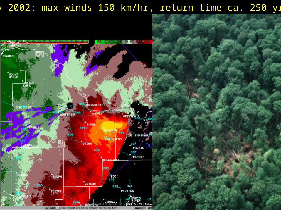
21 July 2002: max winds 150 km/hr, return time ca. 250 yr

Dukes RNA

Initial assessment: consistent with inferences from initial results

- Acer and Fagus, low base-line mortality, high storm mortality;

- Reverse pattern for Betula

- base-line mortality hyper-dispersed, storm mortality strongly clustered, producing gaps of ~30 m).

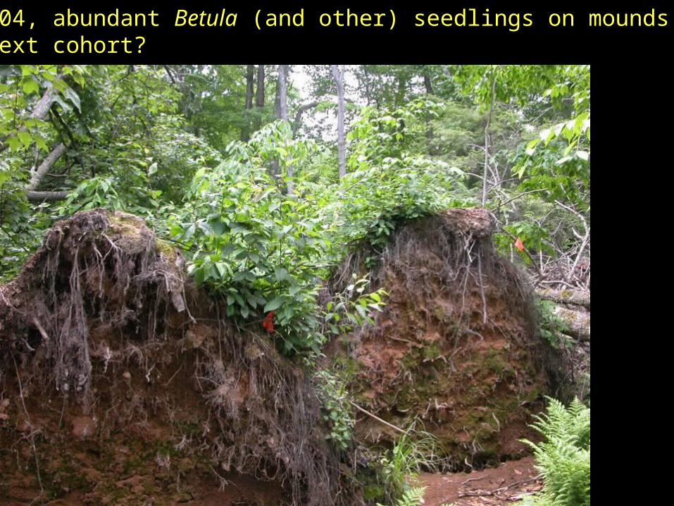
By 2004, abundant Betula (and other) seedlings on mounds.The next cohort?

Plot trajectories: 1935-2004

NMS Axis One

-2.0 -1.5 -1.0 -0.5 0.0 0.5 1.0 1.5

NM

S A

xis

Tw

o

-1.5

-1.0

-0.5

0.0

0.5

1.0

1.5

2.0

SO, some ‘predictability’ at population level. But evidence of coherent pattern at community level?

Acer

Fagus

Tsuga

UPLAND PLOTS ONLY

- In full species-space, Mantel test suggests significant predictability, but - Apparent coherence low in ordination space

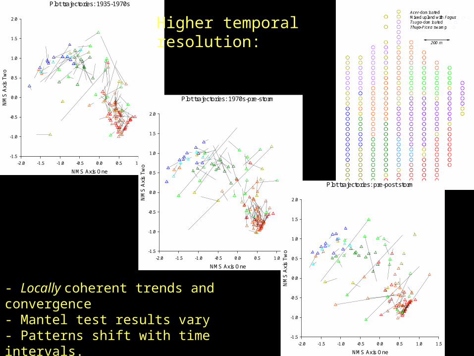
Plot trajectories: 1935-1970s

NMS Axis One

-2.0 -1.5 -1.0 -0.5 0.0 0.5 1.0 1.5

NM

S A

xis

Tw

o

-1.5

-1.0

-0.5

0.0

0.5

1.0

1.5

2.0

Plot trajectories: 1970s-pre-storm

NMS Axis One

-2.0 -1.5 -1.0 -0.5 0.0 0.5 1.0 1.5

NM

S A

xis

Tw

o

-1.5

-1.0

-0.5

0.0

0.5

1.0

1.5

2.0

Plot trajectories: pre-post storm

NMS Axis One

-2.0 -1.5 -1.0 -0.5 0.0 0.5 1.0 1.5

NM

S A

xis

Tw

o

-1.5

-1.0

-0.5

0.0

0.5

1.0

1.5

2.0

Higher temporal resolution:

- Locally coherent trends and convergence - Mantel test results vary- Patterns shift with time intervals.

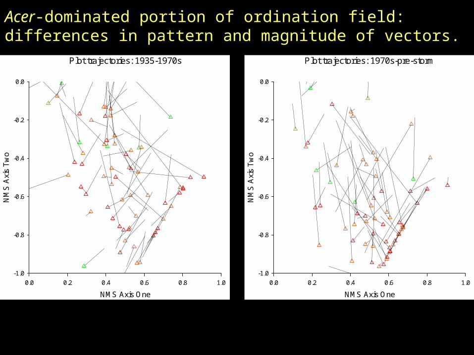
Acer-dominated portion of ordination field: differences in pattern and magnitude of vectors.

Plot trajectories: 1935-1970s

NMS Axis One

0.0 0.2 0.4 0.6 0.8 1.0

NM

S A

xis

Tw

o

-1.0

-0.8

-0.6

-0.4

-0.2

0.0

Plot trajectories: 1970s-pre-storm

NMS Axis One

0.0 0.2 0.4 0.6 0.8 1.0

NM

S A

xis

Tw

o

-1.0

-0.8

-0.6

-0.4

-0.2

0.0

NMS ordination, swamp plots, 1935-1970s

NMS Axis One

-1.5 -1.0 -0.5 0.0 0.5 1.0 1.5 2.0 2.5

NM

S A

xis

Tw

o

-2.0

-1.5

-1.0

-0.5

0.0

0.5

1.0

1.5

NMS ordination, swamp plots, 1970s - current

NMS Axis One

-1.5 -1.0 -0.5 0.0 0.5 1.0 1.5 2.0 2.5

NM

S A

xis

Tw

o

-2.0

-1.5

-1.0

-0.5

0.0

0.5

1.0

1.5

2.0

But little evidence of coherent trajectories in swamp forests.(Mantel test, p=.07, .03)

Thuja

Are different areas or types behaving differently? MRPP comparisons of change vectors

1935-1970s

1970s-2000

City-block distance

0 2 4 6 8

Fre

que

ncy

0.00

0.02

0.04

0.06

0.08

1935

1997-2001

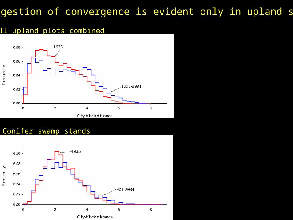
Are plot trajectories convergent?Convergence should change distribution of inter-plot distances in species-space.

City-block distance

0 2 4 6 8

Fre

quen

cy

0.00

0.02

0.04

0.06

0.08

0.10 1935

2001-2004

But suggestion of convergence is evident only in upland stands

All upland plots combined

Conifer swamp stands

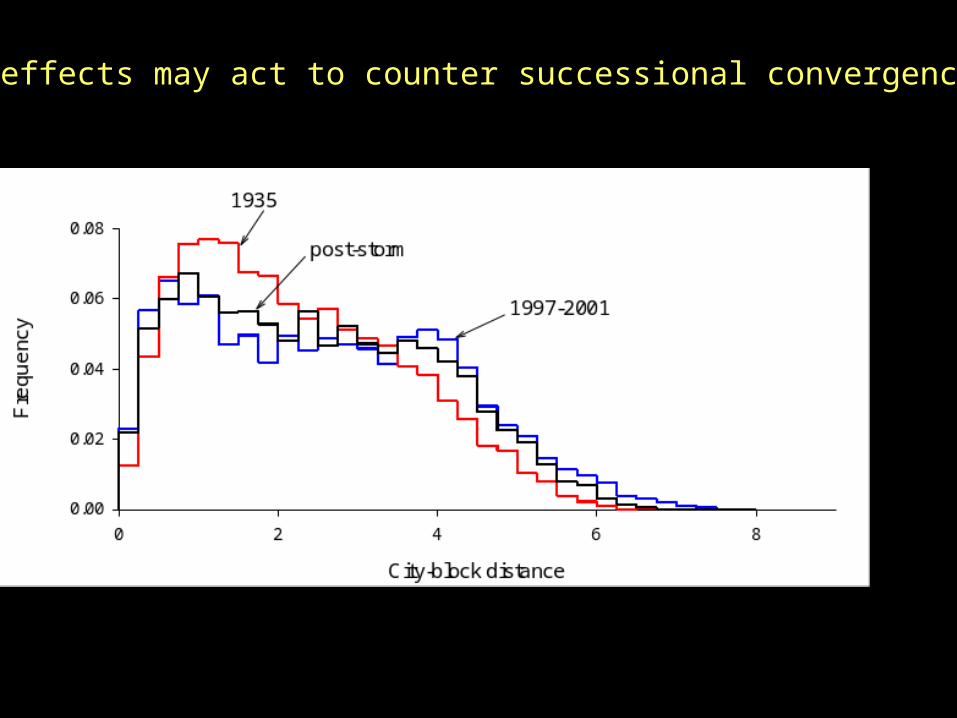
Storm effects may act to counter successional convergence

Summary of ecological results:

- Ancient forests, with no recent disturbance, can be dynamic.

- Dynamics can be influenced by site-conditions, current composition, and infrequent historical events, and all of these factors interact.

- Changes may be predictable at stand scale as results of competitive relationships and environmental change. BUT Current composition relatively weak predictor of trajectories at plot scale.

Methodological and conceptual needs and challenges:

- spatial and temporal scale and resolution are important.

- Historical data sets are of critical value-- but inherited sampling design may constrain how questions can be addressed

SO

- Need data management and analysis tools capable of dealing with variable sampling protocols and intervals and other ‘inherited’ problems with historical data.

- Need focus on development and evaluation of analytical tools for assessing relationships in multi-dimensional data sets over variable scales.

National Science Foundation, Andrew W. Mellon Foundation, US Forest Service, Huron Mt. Wildlife Foundation for support

Thanks to:

Fred Metzger, Eric Bourdo, Jan Schultz for sharing data

AND MANY Bennington College undergraduates for doing the work.

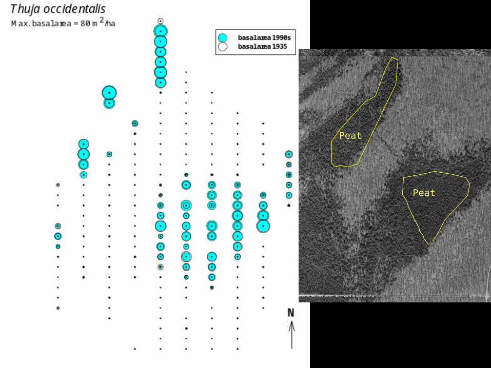
Peat

Peat

Monitoring of individualsallows further demographic insights: growth rates and mortality related.

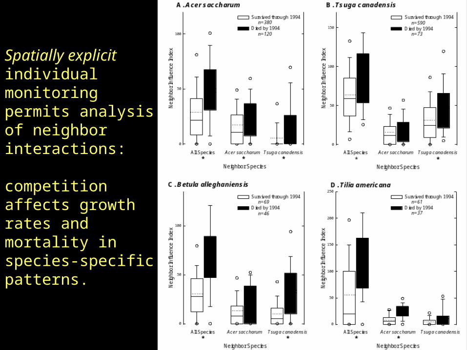
Spatially explicit individual monitoring permits analysis of neighbor interactions:

competition affects growth rates and mortality in species-specific patterns.

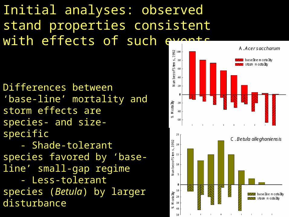
Initial analyses: observed stand properties consistent with effects of such events

Differences between ‘base-line’ mortality and storm effects are species- and size-specific - Shade-tolerant species favored by ‘base-line’ small-gap regime - Less-tolerant species (Betula) by larger disturbance

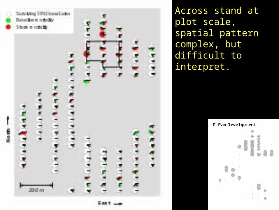
Across stand at plot scale, spatial pattern complex, but difficult to interpret.

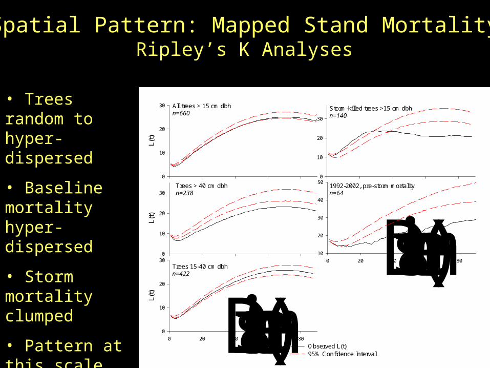
All trees > 15 cm dbhn=660

L(t)

0

10

20

30

Observed L(t)95% Confidence Interval

Storm-killed trees >15 cm dbhn=140

0

10

20

30

Trees > 40 cm dbhn=238

L(t)

0

10

20

30

Trees 15-40 cm dbhn=422

Distance (m)

0 20 40 60 80

L(t)

0

10

20

30

1992-2002, pre-storm mortalityn=64

Distance (m)

0 20 40 60 80

10

20

30

40

50

Spatial Pattern: Mapped Stand MortalityRipley’s K Analyses

• Trees random to hyper-dispersed

• Baseline mortality hyper-dispersed

• Storm mortality clumped

• Pattern at this scale not detectable from plot data

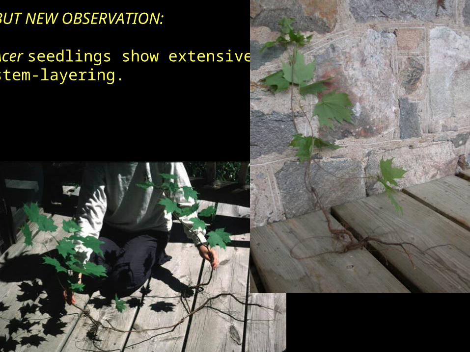
BUT NEW OBSERVATION:

Acer seedlings show extensivestem-layering.

Can layered seedlingsbe released to becomeviable saplings?

YES

In fact, most saplings in‘regeneration patches’appear to have been layered.

SO,- fitness payoff for long- persisting seedlings even greater?- episodic, patchy dynamics even more fundamental?

Even where deer destroy regeneration in smallgaps, large gaps may offer episodic, local escape from browse.