NBER WORKING PAPER SERIES

ARE FREE TRADE AGREEMENTS CONTAGIOUS?

Richard BaldwinDany Jaimovich

Working Paper 16084http://www.nber.org/papers/w16084

NATIONAL BUREAU OF ECONOMIC RESEARCH1050 Massachusetts Avenue

Cambridge, MA 02138June 2010

We would like to thank the useful comments and suggestions of Jean-Louis Arcand, Patricio Aroca,and participants of seminars organised by the Swiss Trade Economist Cooperative (STEC), GraduateInstitute (Geneva), World Trade Organization (WTO), Hitotsubashi University, European EconomicAssociation, Latin American and Caribbean Economic Association (LACEA), Universidad de Chile,and Universidad Catolica del Norte (Antofagasta). The views expressed herein are those of the authorsand do not necessarily reflect the views of the National Bureau of Economic Research.

NBER working papers are circulated for discussion and comment purposes. They have not been peer-reviewed or been subject to the review by the NBER Board of Directors that accompanies officialNBER publications.

© 2010 by Richard Baldwin and Dany Jaimovich. All rights reserved. Short sections of text, not toexceed two paragraphs, may be quoted without explicit permission provided that full credit, including© notice, is given to the source.

Are Free Trade Agreements Contagious?Richard Baldwin and Dany JaimovichNBER Working Paper No. 16084June 2010JEL No. F13

ABSTRACT

This paper presents a new model of the domino effect which is used to generate an empirical indexof how “contagious” FTAs are with respect to third nations. We test our contagion hypothesis togetherwith alternative specifications of interdependence and other political, economical and geographicaldeterminants of FTA formation. Our main finding is that contagion is present in our data and is robustto various econometric specifications and samples.

Richard BaldwinGraduate Institute, GenevaCigale 21010 Lausanne Switzerlandand CEPRand also NBERbaldwin@graduateinstitute.ch

Dany JaimovichGraduate Institute, Geneva132 rue de Lausanne1202 Geneva SwitzerlandDany.Jaimovich@graduateinstitute.ch

1

Are Free Trade Agreements Contagious?

Richard Baldwin and Dany JaimovichF

* Graduate Institute, Geneva

First draft: 23th September, 2008. This version: 9th June, 2010

ABSTRACT This paper presents a new model of the domino effect which is used to generate an empirical index of how “contagious” FTAs are with respect to third nations. We test our contagion hypothesis together with alternative specifications of interdependence and other political, economical and geographical determinants of FTA formation. Our main finding is that contagion is present in our data and is robust to various econometric specifications and samples.

Keywords Contagion Effect, Free Trade Agreements and International Trade

JEL Codes F13

1. 0BINTRODUCTION Regionalism is sweeping the world trade system like wildfire while WTO talks advance at a glacial rate – an unconditional correlation that is often used to suggest that regionalism is a threat to the multilateral trading system (Bhagwati 2008). This concern has prompted a wave of research on why nations are so eager to remove barriers bilaterally.

The most common theoretical explanation in recent decades is “slow multilateralism”, i.e. the assertion that regionalism is spreading because multilateral talks are progressing so slowly (Krugman 1991, Bhagwati 1993, 2008). Another set of explanations turn on idiosyncratic events, such as the US’s opening of the US-Canada FTA talks in 1986 (Bhagwati 1991 p.71), the breakup of the USSR in 1991 (Lester and Mercurio 2009 p.3), and the Asian Crisis of 1997 (Harvie, Kimura and Lee 2006 p.3). More institutional explanations for regionalism’s popularity include the global spread of democracy (Mansfield, Milner, and Rosendorff 2002, Wu 2004), and the quest for geopolitical stability (Mansfield and Pevehouse 2000, Martin et al. 2008, 2010, and Vicard 2008).

* We would like to thanks the useful comments and suggestions of Jean-Louis Arcand, Patricio Aroca, and participants of seminars organised by the Swiss Trade Economist Cooperative (STEC), Graduate Institute (Geneva), World Trade Organization (WTO), Hitotsubashi University, European Economic Association, Latin American and Caribbean Economic Association (LACEA), Universidad de Chile, and Universidad Catolica del Norte (Antofagasta).

2

One lacuna in these hypotheses is the lack of recognition of third-nation effects, i.e. FTA interdependence. This angle is stressed by the so-called bandwagon or emulation arguments that posit a link between FTAs signed by the ‘trade giants’ (US, EU and Japan) and the attitudes of other nations. The giants’ FTAs create “a sense elsewhere that regionalism is the order of the day and others must follow suit” (Bhagwati 1991 p.73, and, more recently, Solis, Stallings and Katada 2009). The political economy logic of this assertion has not been fully worked out but the idea seems a general ‘demonstration effect’. A related line of thinking for which the political economy links have been worked out is the domino theory of regionalism formalized in Baldwin (1993).F

1F This argues that

the signing or deepening of one FTA can induce excluded nations to sign new FTAs that were previously shunned. The logic turns on the way that trade diversion creates new political economy forces in excluded nations. Specifically, excluded nations seek to sign FTAs as a means of redressing the new discrimination. The second-round FTAs in turn create their own trade diversion that may in turn lead to more FTAs. Using an obvious metaphor, the domino theory explains why FTAs seem to be ‘contagious’.

Our paper aims to crystallize the domino-effect logic with respect to bilateral FTAs and to test it in a broad panel of countries. The empirical linkages have already been established in a more reduced form setting by Egger and Larch (2008) using spatial econometric methods.

The value added of our paper is threefold. First, we extend the domino theory model to allow for FTAs (the original contributions concerned customs unions). Second, we use the model to develop a theory-based measure of contagion. Importantly, our measure of contagion captures asymmetries in the dyads, while Egger and Larch (2008) implicitly assume contagion is bilaterally symmetric (since their measure depends on distance). Third, we test the domino-effect against alternative hypotheses using a broader sample of FTAs than previous studies. The key empirical lever that allows us to distinguish them from the contagion is the extent to which trade ties connect the new FTA signers. The contagion hypothesis works on trade diversion, so the spread of FTAs should follow a pattern that is clearly related to the new signers’ trade patterns. In particular, a pair of nations should be more likely to sign a new FTA if either of them has recently signed FTAs with third nations that are the pair’s exporting rivals.

The rest of the paper is organized as follows. The next section reviews the literature and the subsequent one presents our model. Next we present our empirical strategy, data and results. The final section presents our concluding remarks. 1 There are precedents. Whalley (1993) informally argues that Western Hemispheric regionalism was largely defensive, focusing on fears of US aggressive unilateralism instead of trade diversion; he also does not posit a circular causality between bloc size and the strength of inclusionary pressures. Hufbauer (1989) uses the term “FTA magnetism” which captures the first step (idiosyncratic deepening sparks membership requests) but does not relate the strength of the magnetism to the bloc size. Winters (1996) and Lawrence (1996) surveys regionalism and multilateralism models, putting the domino theory in perspective. See Baldwin (1994, 1997, 2008) for applications to, respectively, the waves of regionalism in Europe, the Western Hemisphere, and East Asia.

3

2. 1BLITERATURE REVIEW 2.1. 11BTheoretical work on FTA formation A wide range of theory articles have studied the incentive to form or join FTAs. The first paper to consider endogenous customs union formation seems to be Riezman (1985). He works in a 3-nation Walrasian setting, assuming that international transfers are impossible but that nations’ can violate their GATT/WTO commitments by raising external tariffs after a customs union is formed. He formally shows that many unexpected results can occur depending upon exogenous national asymmetries. For example, he shows that a customs union may be stable between nations even though they would both be better off under global free trade. A very different approach is the domino theory of regionalism (Baldwin 1993). Working with a monopolistic competition trade model, he shows that the trade-diversion effects of customs union formation can induce nations that were previously against membership to change their minds and join. Moreover, the pure economic incentive of excluded nations to join rises with customs union membership. If the membership expansion is spread over time for practical reasons, a single event of regionalism may appear to spark a domino-like chain reaction where each new membership triggers another. The result may be global free trade if nations’ intrinsic resistance to joining is not too great.

Yi (1996), working with a version of the Brander-Krugman model of oligopolistic firms facing segmented markets, applies standard game theoretic analysis of coalition structures to study the domino effect more formally. He shows that the global free trade outcome (the grand coalition) is stable when membership is open, but not necessarily when incumbents can veto enlargement. Krishna (1998) also works with the Brander-Krugman model of trade and symmetric nations, but assumes governments’ FTA choices are only affected by their firms’ operating profit. He studies the interests that countries have in forming an FTA, showing that nations of similar size are likely to gain from the FTA. He also shows that FTAs which produce a great deal of trade diversion are especially beneficial to the FTA partners. Freund (2000), working with a Brander-Krugman like model where every firm sells to every market, shows that any two nations would gain from forming an FTA as long as the MFN tariff was below the optimal tariff level. Note that trade bloc formation in this sort of oligopoly model shifts pure profits to the bloc at the expense of third nations. Multilateral free trade would eliminate the bloc’s advantage, so analyses based on such models tend to produce endogenous bloc sizes that do not include all nations, i.e. the trade blocs are stumbling blocks to global free trade.

Aghion, Antras and Helpman (2007) use cooperative game theory to analyse FTA formation. So as to be able to directly employ well-known game theoretic results, they apply to nations assumptions which are standard when modelling cooperative games among private agents. Specifically, they assume that one nation is the undisputed agenda setter, and that unlimited transfers among nations are possible and costless (transferable utility). Under these strong assumptions they are able to formally show that almost anything can happen, including an outcome that resembles the domino effect.

4

2.2. 12BEmpirical studies of FTA formation Empirical studies of FTA formation are much rarer as FTA membership is typically taken as exogenous by empirical researchers.

A first systematic empirical study on the economical determinants of FTAs is Baier and Bergstrand (2004). This paper, however, does not consider any of the hypotheses accounting for the spread of FTAs. The authors use cross-section data to estimate a linear probability model linking ‘economic’ factors to the choice of FTAs. In particular, they find that the likelihood of an FTA between a country pair is higher the closer they are, the more distant from the rest of the world, the larger and more similar their economic size are and the more different their labour ratios are. The authors argue that these factors explain which FTA would lead to the greatest welfare gains.

Several empirical studies have focused on aspects beyond the economic determinants. Mansfield and Reinhardt (2003) offer a political explanation, providing empirical support for the “slow multilateralism” argument and other developments at the GATT/WTO as key explanations. Mansfield, Milner, and Rosendorff (2002) empirically find that pairs of democratic countries are more likely to form an FTA, a result confirmed by Wu (2004), who also claims that economic and trade uncertainty matter. Holmes (2005) shows “mercantile interests” in assuring export market access are also important determinants. The first evidence of the geopolitical stability hypothesis is Mansfield and Pevehouse (2000), who show that countries with an FTA are less likely to have a war, a result formally explained in Martin et al. (2008) and tested in Martin et al. (2010) and Vicard (2008).

FTA interdependence has received little empirical attention. The first efforts are attempts to prove the domino theory in the European context. Sapir (1997) estimates year-by-year gravity equations to identify the trade diversion effect of the EU on non-members. He finds that trade diversion estimates tend to spike just in advance of EU enlargements and suggests that the enlargements were caused by the heightened trade diversion. Baldwin and Rieder (2007) undertake a similar procedure as a first stage to identify trade diversion and add a second stage that estimates a linear probability model linking the likelihood of joining the EU to contemporaneous trade diversion. This procedure, however, is plagued by the endogeneity of the membership decision in the first stage. An early use of the spatial econometric techniques in the FTA study is Manger (2006). Building a weight matrix based in the average geographical distances of the countries in the involved dyads, he provides evidence of spatial dependence. Egger and Larch (2008), using a similar weighting strategy, extend the spatial econometric analysis to the study of dynamic FTA formation and enlargement and incorporate long term implications of interdependence in a cross-section analysis estimated with Bayesian techniques.

3. 2BTHEORETICAL CONSIDERATIONS The formal domino theory presented in Baldwin (1993) applies to the analysis of an expanding customs union, not FTAs. In the case of a customs union, the choice is simply to be in or out. The analysis, however, must be quite different when considering bilateral FTAs as the lack of a common external tariff changes the analysis fundamentally. The key domino result concerns the way a third party FTA can switch a nation’s decision to

5

sign a particular FTA from ‘no’ to ‘yes.’ The fulcrum of the modelling is therefore the comparison of the Home government’s objective function when it chooses to stay with MFN trade policy versus when it chooses to sign an FTA with, say, nation-j. The domino effect is said to arise when an FTA between nation-j and a third nation makes the Home government more likely to sign the FTA with nation-j when previously it preferred MFN trade policy. This section introduces a model where the domino effect arises with respect to bilateral FTAs.

Endogenising the decision to form an FTA partnership requires an economic model that specifies the effects of trade agreements and a political model that maps the economic effects into policy choices. We turn first to the economic model, keeping it as simple as possible. We conjecture that the domino effect would arise in many other economic settings.

3.1.1. 20BThe economy We assume a world of R countries, each with two sectors: a manufacturing sector (the M-sector) and a numeraire sector (the A sector) and two factors (labour L and capital K). The tastes of all consumers are identical and given by the indirect utility function:

σμσ

σμμ <<<⎟⎠⎞⎜

⎝⎛≡≡=

−

Γ∈

−− ∫ 10,,;)1/(1

11

i iMMA dipPPpPPEV (1)  

where E is the typical nation’s expenditure, P is the ideal price index, pA is the price of A, pi is the consumer price of manufacturing variety i (the variety subscript is dropped where clarity permits), μ is the expenditure share on all varieties, Γ is the set of varieties available for consumption, and σ is the constant elasticity of substitution between any two varieties; the regularity conditions on μ and σ are maintained throughout the analysis. Demand for variety-j sold in a typical market is thus:

σ−1

MP

σ μ−

≡ jj

Epc (2)  

The basic features of this sort of trade model are well known, so we move quickly through the analysis (see Appendix 1 for details).

The A-sector assumptions are designed to permit analysis of trade in manufactures with as few confounding factors as possible. Specifically, it is marked by perfect competition, constant-returns and uses only labour; its output is costlessly traded. Consumers facing X(1)X demand good-A according to: CA=(1-μ)E/pA. Perfect competition forces marginal cost pricing, so pA=aAw in all nations, where aA is the unit labour input coefficient. Costless trade equalises pA globally and thus equalises wage rates in all nations (as long as the nations are sufficiently similar in size to ensure that some A-good is made in all regions, an assumption maintained throughout). Taking A as numeraire and choosing units such that aA=1, the law of one price in good A implies w=1 in all nations.

The M-sector is subject to Dixit-Stiglitz monopolistic competition and increasing returns of the fixed-cost-and-constant marginal-cost type. The fixed cost comprises only K (one unit of K per variety) while the marginal cost comprises only L (aM units of L per unit of output).

6

While nations’ labour supplies are fixed, capital is assumed to be constructed using labour and it is assumed to depreciate in a ‘one horse shay’ manner, i.e. it works perfectly until it dies – an event that occurs according to a Poisson process with a hazard rate of δ. In the long run, the capital stock in each nation rises to equate its long-run equilibrium reward, namely (ρ+δ)F, where ρ is the discount rate, δ is the hazard rate, and F is the fixed cost of producing the unit of capital that every variety requires (see Appendix). In short, entry in reaction to a rise in π is fast (instantaneous) but exit is slow (governed by a Poisson ‘death’ process); see Appendix for details.

As usual, a constant mark-up and ‘mill pricing’ are optimal, so choosing units such that aM = (1-1/σ) and using w=1, the consumer price of a good produced in origin nation ‘o’ and sold in destination nation ‘d’ is:

ododp τ= (3)  

where τod is one plus the ad valorem tariff on goods sold from nation-o to nation-d (of course, τoo=1).

The constant mark-up pricing means that a firm’s operating profit is 1/σ times its revenue. Employing X(2)X and X(3)X, a typical firm based in nation-o earns operating profit on its sales to nation-d (we denote this as πod) equal to:

w

w

d

Edodod n

Esσμφ

πΔ

≡ (4)  

where the bilateral “freeness of trade parameter”, φod ≡ (τod)1-σ, applied against exports from nation-o to nation-d rises from zero (when the tariff is infinite) to unity (when bilateral trade is perfectly free); also

donn

ssEE

s oowi

niR

i idnidwi

Ei ,1,,,1

∀≡≡≡Δ≡ ∑ =φφ

Here Ei and ni are nation-i’s expenditure and the number (mass) of symmetric varieties produced, Ew and nw are the world totals of expenditure and varieties, and Δ is a weighted average of the bilateral trade freeness parameters where national shares of nw are the weights. Summing πod across all markets, operating profit of a typical o-based firm is:

∑ = Δ

R

dd

Edodwo

s

nE=

1

φσμπ

w

(5)  

Since capital is used only as the fixed cost, πo is the reward to capital in nation-o. Instant entry and slow exit implies that the steady state reward is:

F

nE

w )( δρσμ

+=w

(6)  

3.1.2. 21BThe political economy model Our political economy model is designed to capture the tendency of nations to sign ‘defensive’ FTAs, i.e. to seek preferential trade agreements that offset emerging

7

discrimination. The key modelling assumption concerns the asymmetric nature of lobbying for gains and against losses. There are many ways of modelling this “losers lobby harder” phenomenon, perhaps the most famous being the “conservative social welfare function” of Corden (1974). The modelling approach we adopt – an approach that turns on sunk market entry costs – is that of Baldwin and Robert-Nicoud (2007). In our economic model, firms enter quickly but exit slowly, so incumbent manufacturing firms cannot benefit from lobbying for pure gains – in the sense of raising their operating profit above the equilibrium rate. The reason is that these gains would be instantly arbitraged away by new entrants, leaving the incumbents with the lobbying cost and zero benefit. Incumbents can, by contrast, benefit from lobbying when faced with pure losses. The reason is that the sunk entry-cost creates quasi-rents that can be exploited without inducing entry. (See Appendix 1 for a full exposition of entry and the exit in the model.)

More specifically, any π > (ρ+δ)F is instantly eliminated by free entry, but when π < (ρ+δ)F firms exit according to the Poisson death process where δ is the hazard rate. This slow exit creates the possibility of quasi-rents, i.e. the possibility that π can be raised up to it long-run rate without attracting entry. Firms lobby for changes in trade policy in order to obtain these quasi-rents, i.e. to push their operating profit back to its normal level. (See Baldwin and Robert-Nicoud 2007 for a detailed treatment of this political economy effect.)

Apart from the asymmetric treatment of above-normal and below-normal operating profit, the political economy model is standard. As in Grossman and Helpman (1994), the government chooses trade arrangements to maximise a weighted objective function, where the weights apply to, respectively, the utility of income derived from labour income, capital owners’ quasi-rents and tariff revenue.F

2F The typical government’s

objective function is:

( )[ ]oi

R

io

oooooo Z

PTRFnLw

G ∑ =−⎟⎟

⎠

⎞⎜⎜⎝

⎛ ++−+=

1

)( χδρπβα (7)  

where Po is nation-o’s price index, and α, β and χ are the weights on labour, quasi-rents and tariff revenue (denoted as TR), and the Z’s are the idiosyncratic political costs nation-o’s government faces when signing a free trade agreement with nation-i (this may be positive or negative depending upon how nation-o voters view each possible FTA). Due to our assumptions on fast entry and slow exit, the maximum of the term in square brackets is zero.

27BTrade diversion as a political economy force The core mechanism in the model is the domino or contagion effect of third-nation FTAs. To illustrate this, we consider R=3, and an initial situation where all three nations are symmetric in size and trade policy. To keep the reasoning concrete, we study the decision of nation-1 to sign a free trade agreement with nation-2. To start the analysis, we

2 Grossman and Helpman (1994) derive this assuming that every organised lobby signs an enforceable contract with the government whereby the lobby pays money to the government in exchange for tariffs according to a specific schedule.

8

determine the baseline level of nation-1’s objective function and establish conditions under which no FTA would be signed. To simplify the formulas, we join Krishna (2003) in assuming that α = χ = 0 and β = 1 inX(7)X, so only quasi-rents matter.

By symmetry in the initial situation, each nation has a third of world M-sector firms. The usual features of Dixit-Stiglitz competition imply that operating profit globally is μEw/σ, where Ew is world expenditure. Given free entry, the number of varieties worldwide, nw, must adjust to equate the reward to capital, μEw/σnw, to its equilibrium rate, (ρ+δ)F. Plainly then the middle term in X(7)X is initially zero. With α = χ = 0 and β = 1:

01 =MFNG (8)  

This is the baseline level of the objective function that nation-1’s government will use when deciding whether to sign an FTA with nation-2. Here the superscript indicates the case using an obvious notation.

Next consider whether nation-1 would sign an FTA with nation-2. To begin with, we consider the short run effects, i.e. when the number of varieties in each nation is fixed at 1/3 of the world’s total. In this case, straightforward manipulation of the Dixit-Stiglitz monopolistic competition equilibrium when nations 1 and 2 form an FTA but all other trade flows are subject to MFN tariffs implies:

ww nE

nE =

σμ

φφσφφμπ >

)+)(22+(1)+6+(2FTA12

1

ww 2

12FTA12

1 ZG −=

Comparing this to X(6)X, we see that operating profit for nation-1 firms has risen above its equilibrium level (with the same being true for nation-2). This will attract entry, so there will be no quasi-rents to affect the government’s decision. Using these facts in X(7)X and adding in the idiosyncratic political-resistance factor, the objective function’s value is:

(9)  

Assuming Z12 is positive (i.e. there is some intrinsic resistance to economic integration), the nation-1 government will not ask for nor accept an FTA with nation-2. By symmetry, neither will any nation, so the initial MFN trade policy is a stable policy equilibrium.

To move away from this MFN situation, the system needs a shock and we model this as a change in the parameters of intrinsic resistance to FTAs, i.e. the Z’s. Specifically, we assume that, for reasons not addressed in the model, the intrinsic resistance to an FTA between nations 2 and 3 switches sign, so nations 2 and 3 find it politically optimal to sign an FTA even though it was not politically optimal to do so before the shock.

Our task is to show that this exogenous FTA formation alters the political optimality of an FTA between nations 1 and 2. To preview the political economy logic, note that the new FTA will lower the operating profit of firms in nation-1 due to trade diversion. This, in turn, creates quasi-rents that enter into government 1’s objective function. As we shall see, this may switch the nation-1’s attitude towards an FTA with nation-2.

After the formation of the nation 2 and 3 FTA, and again focusing on the short run, X(3)X and X(5)X imply that the operating profit of a typical nation-1 firm is:

9

w

w

w

w

nE

nE =

σμ

φφσφφμπ <

)+)(22+(1)4+3+(2 2

FTA231

By inspection, operating profit is less than it was in the MFN baseline, so the trade diversion has created quasi-rents. These enter nation-1’s objective function, so it is now:

0

3)21(1

)+)(22+(1)4+3+(2 12

FTA231 <⎟⎟

⎠

⎞⎜⎜⎝

⎛ +⎟⎟⎠

⎞⎜⎜⎝

⎛−=

−σφφφ

φφσμ w

w

w nnEG

μ

12FTA23

123&FTA12

1 ZGG >−

(10)

The FTA between nations 2 and 3 raises the operating profit of their firms; the resulting entry will depress nation-1 operating profits even further. (See Appendix 1 for the precise formulas.)

Importantly, the nation 2 and 3 FTA has deleted the MFN status quo equilibrium. The negative level of the nation-1’s objective function shown in X(10)X is the new baseline against which the nation-1 government will judge the impact of an FTA with nation-2. Or to put it differently, the attractiveness of signing with nation-2 is boosted by considerations that did not enter the calculation before nation-1’s trade partners signed an FTA. The FTA with nation 2 is more attractive now because it allows the nation-1 government to redress its firms’ losses. More formally, nation-1 will sign an FTA with nation-2 as long as:

where the superscript “FTA12&23” indicates the situation when there are FTAs between nations 1 and 2 as well as between 2 and 3. Plainly, the fact G1

FTA23 is negative makes it more likely for the inequality to hold.

Performing the short-run calculations, we see that:

w

w

w

w

nE

nE =

σμ

φσφμπ <)+3(2)4+(523&FTA12

1

so that operating profit is still below the equilibrium value. F

3F This means that the new

FTA does not fully offset the discrimination faced by nation-1 firms. In other words, nation-1 would rather return to the baseline of global MFN trade than sign an FTA with nation-2, but it no longer has that choice. Calculating the short-run price index in this case, the implied level of the objective function is:

0

3)2(1

)+3(2)4+(5 1

23&FTA121 <⎟⎟

⎠

⎞⎜⎜⎝

⎛ +⎟⎟⎠

⎞⎜⎜⎝

⎛−=

−σμ

φφφ

σμ w

w

w nnEG

(11)

3 By symmetry, the same is true for nation-3, but nation-2, which is the hub in this hub-and-spoke arrangement, enjoys higher operating profit and so some firms would enter. This would further depress π1 and π2.

10

When evaluating nation-1’s choice, the key is whether X(11)X is less than X(10)X. If this is true, nation-1 will embrace an FTA with nation-2 as long as the intrinsic resistance Z12 is not too large. To rank X(10)X and X(11)X we study their ratio, which can be shown to equal:

121

221

6 1<⎟⎟

⎠

⎞⎜⎜⎝

⎛++

+

−σμ

φφ

φφ

What this means is that G1

FTA12&23 is indeed less negative than G1FTA23, so nation-1 will

embrace an FTA with nation-2 after nation-2 has signed an FTA with nation-3, provided that Z12 is not too large. (See Appendix 1 for the precise formulas when we allow for instant entry in nations 2 and 3; the qualitative results are not affected.)

3.1.3. 22BDeriving a contagion index The preceding analysis makes it clear that the linchpin of the domino effect is the way an FTA between a nation’s partners harm its exporters’ operating profit. In the example studied, the domino effect stemmed from the impact on nation-1’s operating profit of freer trade between nations 2 and 3. It is impossible to calculate this analytically for general patterns of bilateral tariffs (the sni’s cannot be solved for a general R and general pattern of φ’s). We can, by contrast, derive the impact of a marginal change in third-nation trade freeness and we propose this as a way of operationalising, on real data, the strength of the domino effect arising from any given FTA.

Differentiating X(5)X for nation-1 with respect to reciprocally freer trade between nations j and k, we have:

⎟⎟⎠

⎞⎜⎜⎝

⎛

Δ

−

Δ+

Δ−

Δ jkk

nj

k

Ejkj

j

nk

j

Ejw

w

dss

dss

nE =d φ

φφ

φ

σμπ )()( 1k1j

1 (12)

While the preferential liberalisation between nations j and k is reciprocal in the case of an FTA, we can think of it as two separate changes in trade policy – lower tariffs charged by j on imports from k (this is reflected in the rise of φkj) and the lower tariff charged by k on imports from j (this is reflected in the rise of φjk). This allows us to consider the ‘contagion’ coming to nation 1 from nation j and, separately, from nation k. Separating the effects and forming proportional changes for the first, we have:

⎟⎟⎠

⎞⎜⎜⎝

⎛

Δ

−⎟⎟⎠

⎞⎜⎜⎝

⎛

j

kjnk

kjkj

s =

dd φ

ππ

φφππ

1

1j11

//

Note that the first right-hand is the proportion of operating profit that a typical nation-1 firms earns on sales to nation-j. Because operating profits in this model are proportional to sales, we can take the share of nation-1’s exports that go to nation-d as a proxy for the first right-hand term. The second right-hand term is, as inspection of X(2)X reveals, the market share of firms from nation-k in nation-j’s market. We can take j’s import share from k as a proxy for this. Putting these together, and noting that the bilateral φ goes to zero under the FTA, we can approximate the contagion effect from nation-j’s FTAs on nation 1 by:

11

kjFTA ⎟

⎟⎠

⎞⎜⎜⎝

⎛⎟⎟⎠

⎞⎜⎜⎝

⎛≅

j

kj

1

1j1kj imports total

exports bilateral exports total

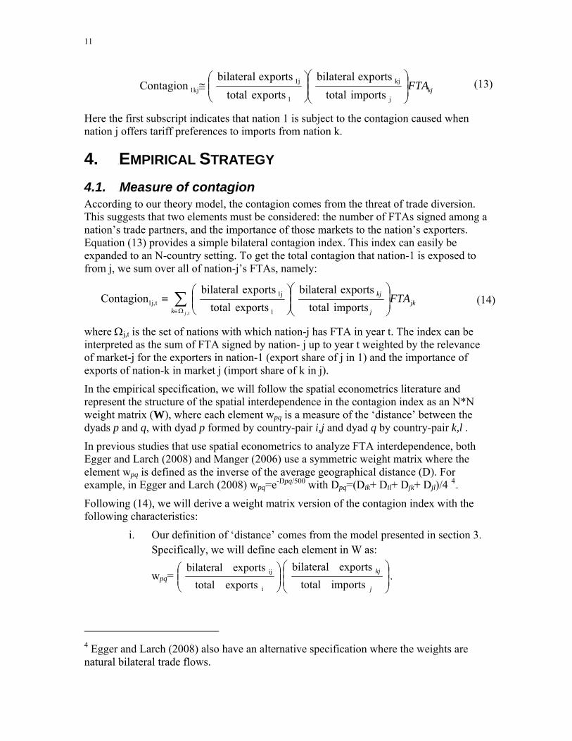
exports bilateralContagion (13)

Here the first subscript indicates that nation 1 is subject to the contagion caused when nation j offers tariff preferences to imports from nation k.

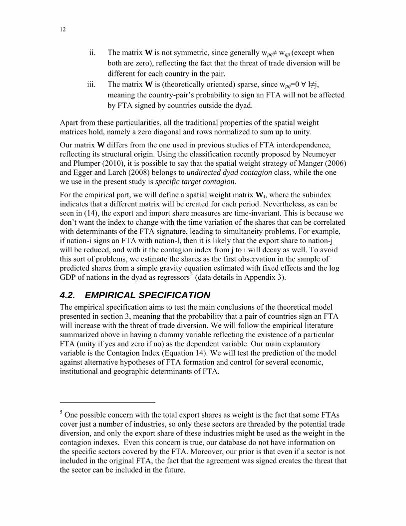
4. 3BEMPIRICAL STRATEGY 4.1. 13BMeasure of contagion According to our theory model, the contagion comes from the threat of trade diversion. This suggests that two elements must be considered: the number of FTAs signed among a nation’s trade partners, and the importance of those markets to the nation’s exporters. Equation (13) provides a simple bilateral contagion index. This index can easily be expanded to an N-country setting. To get the total contagion that nation-1 is exposed to from j, we sum over all of nation-j’s FTAs, namely:

(14)∑

Ω∈⎟⎟⎠

⎞⎜⎜⎝

⎛⎟⎟⎠

⎞⎜⎜⎝

⎛≡

tjkjk

j

kj FTA ,

imports totalexports bilateral

exports totalexports bilateral

Contagion1

1jt1j,

where Ωj,t is the set of nations with which nation-j has FTA in year t. The index can be interpreted as the sum of FTA signed by nation- j up to year t weighted by the relevance of market-j for the exporters in nation-1 (export share of j in 1) and the importance of exports of nation-k in market j (import share of k in j).

In the empirical specification, we will follow the spatial econometrics literature and represent the structure of the spatial interdependence in the contagion index as an N*N weight matrix (W), where each element wpq is a measure of the ‘distance’ between the dyads p and q, with dyad p formed by country-pair i,j and dyad q by country-pair k,l .

In previous studies that use spatial econometrics to analyze FTA interdependence, both Egger and Larch (2008) and Manger (2006) use a symmetric weight matrix where the element wpq is defined as the inverse of the average geographical distance (D). For example, in Egger and Larch (2008) wpq=e-Dpq/500 with Dpq=(Dik+ Dil+ Djk+ Djl)/4 F

4F.

Following (14), we will derive a weight matrix version of the contagion index with the following characteristics:  

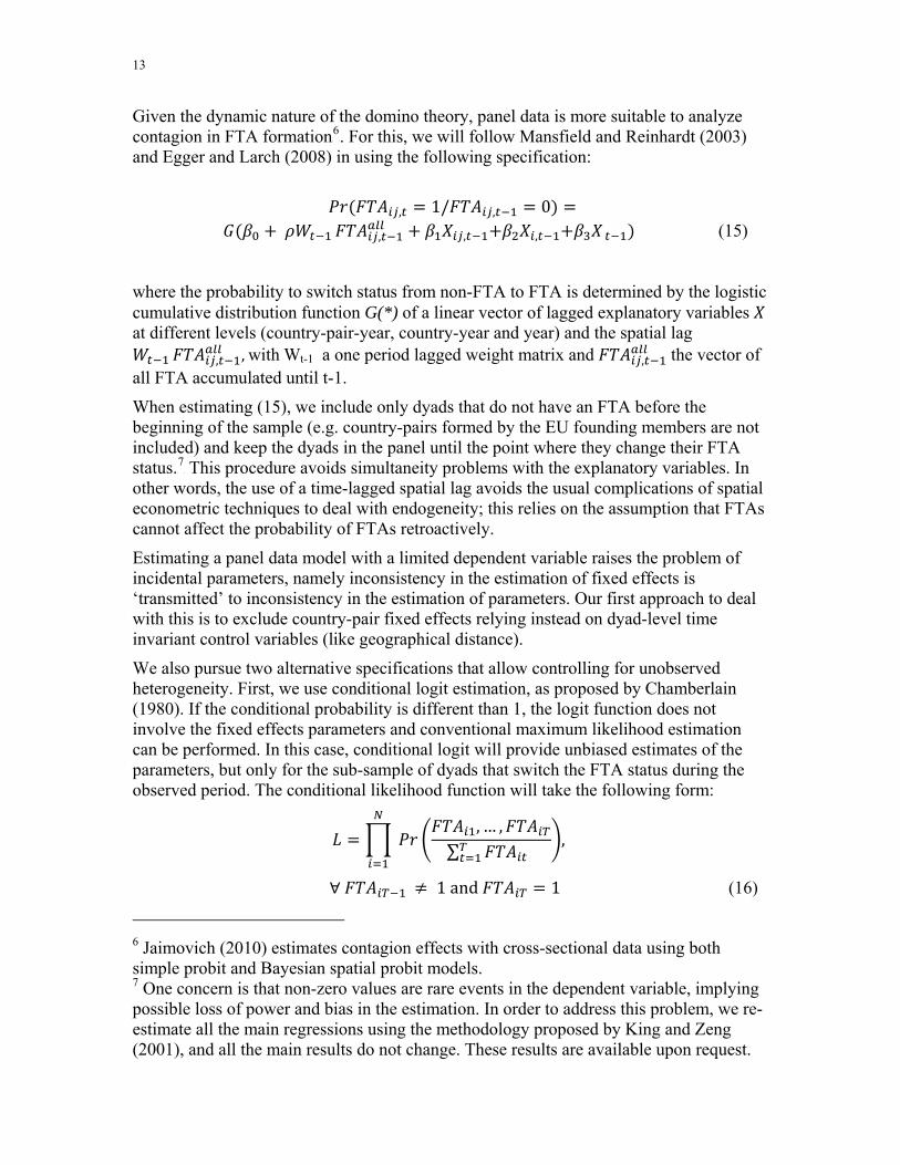
i. Our definition of ‘distance’ comes from the model presented in section 3. Specifically, we will define each element in W as:

wpq=  ⎟⎟⎠

⎞⎜⎜⎝

⎛

i

ij

exportstotalexportsbilateral

⎟⎟⎠

⎞⎜⎜⎝

⎛

j

kj importstotal

exportsbilateral

.

4 Egger and Larch (2008) also have an alternative specification where the weights are natural bilateral trade flows.

12

ii. The matrix W is not symmetric, since generally wpq≠ wqp (except when both are zero), reflecting the fact that the threat of trade diversion will be different for each country in the pair.

iii. The matrix W is (theoretically oriented) sparse, since wpq=0 l≠j, meaning the country-pair’s probability to sign an FTA will not be affected by FTA signed by countries outside the dyad.

Apart from these particularities, all the traditional properties of the spatial weight matrices hold, namely a zero diagonal and rows normalized to sum up to unity.

Our matrix W differs from the one used in previous studies of FTA interdependence, reflecting its structural origin. Using the classification recently proposed by Neumeyer and Plumper (2010), it is possible to say that the spatial weight strategy of Manger (2006) and Egger and Larch (2008) belongs to undirected dyad contagion class, while the one we use in the present study is specific target contagion.

For the empirical part, we will define a spatial weight matrix Wt, where the subindex indicates that a different matrix will be created for each period. Nevertheless, as can be seen in (14), the export and import share measures are time-invariant. This is because we don’t want the index to change with the time variation of the shares that can be correlated with determinants of the FTA signature, leading to simultaneity problems. For example, if nation-i signs an FTA with nation-l, then it is likely that the export share to nation-j will be reduced, and with it the contagion index from j to i will decay as well. To avoid this sort of problems, we estimate the shares as the first observation in the sample of predicted shares from a simple gravity equation estimated with fixed effects and the log GDP of nations in the dyad as regressorsF

5F (data details in Appendix 3).

4.2. 14BEMPIRICAL SPECIFICATION The empirical specification aims to test the main conclusions of the theoretical model presented in section 3, meaning that the probability that a pair of countries sign an FTA will increase with the threat of trade diversion. We will follow the empirical literature summarized above in having a dummy variable reflecting the existence of a particular FTA (unity if yes and zero if no) as the dependent variable. Our main explanatory variable is the Contagion Index (Equation 14). We will test the prediction of the model against alternative hypotheses of FTA formation and control for several economic, institutional and geographic determinants of FTA.

5 One possible concern with the total export shares as weight is the fact that some FTAs cover just a number of industries, so only these sectors are threaded by the potential trade diversion, and only the export share of these industries might be used as the weight in the contagion indexes. Even this concern is true, our database do not have information on the specific sectors covered by the FTA. Moreover, our prior is that even if a sector is not included in the original FTA, the fact that the agreement was signed creates the threat that the sector can be included in the future.

13

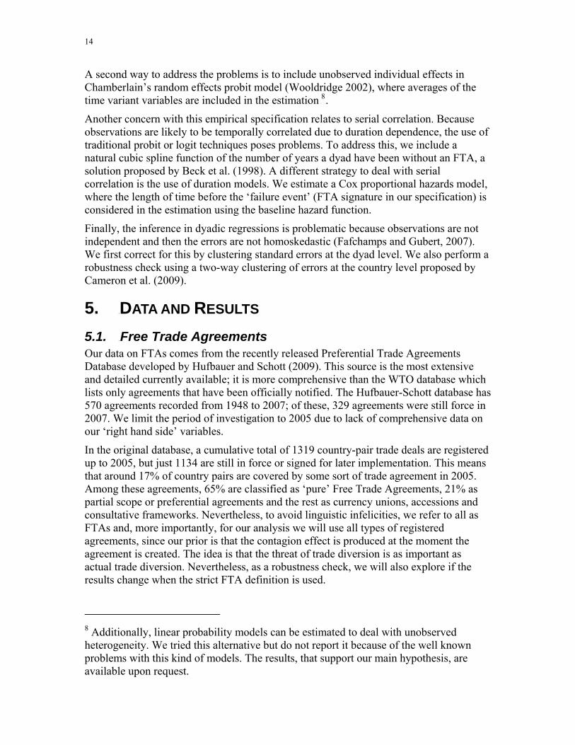
Given the dynamic nature of the domino theory, panel data is more suitable to analyze contagion in FTA formationF

6F. For this, we will follow Mansfield and Reinhardt (2003)

and Egger and Larch (2008) in using the following specification:

  , 1/ , 0

                       , , ,     (15)

where the probability to switch status from non-FTA to FTA is determined by the logistic cumulative distribution function G(*) of a linear vector of lagged explanatory variables at different levels (country-pair-year, country-year and year) and the spatial lag

  , , with Wt-1 a one period lagged weight matrix and ,  the vector of all FTA accumulated until t-1.

When estimating (15), we include only dyads that do not have an FTA before the beginning of the sample (e.g. country-pairs formed by the EU founding members are not included) and keep the dyads in the panel until the point where they change their FTA status.F

7F This procedure avoids simultaneity problems with the explanatory variables. In

other words, the use of a time-lagged spatial lag avoids the usual complications of spatial econometric techniques to deal with endogeneity; this relies on the assumption that FTAs cannot affect the probability of FTAs retroactively.

Estimating a panel data model with a limited dependent variable raises the problem of incidental parameters, namely inconsistency in the estimation of fixed effects is ‘transmitted’ to inconsistency in the estimation of parameters. Our first approach to deal with this is to exclude country-pair fixed effects relying instead on dyad-level time invariant control variables (like geographical distance).

We also pursue two alternative specifications that allow controlling for unobserved heterogeneity. First, we use conditional logit estimation, as proposed by Chamberlain (1980). If the conditional probability is different than 1, the logit function does not involve the fixed effects parameters and conventional maximum likelihood estimation can be performed. In this case, conditional logit will provide unbiased estimates of the parameters, but only for the sub-sample of dyads that switch the FTA status during the observed period. The conditional likelihood func take the following form: tion will

 , … ,

 ∑  , 

                                                      1 and  1 (16)

6 Jaimovich (2010) estimates contagion effects with cross-sectional data using both simple probit and Bayesian spatial probit models. 7 One concern is that non-zero values are rare events in the dependent variable, implying possible loss of power and bias in the estimation. In order to address this problem, we re-estimate all the main regressions using the methodology proposed by King and Zeng (2001), and all the main results do not change. These results are available upon request.

14

A second way to address the problems is to include unobserved individual effects in Chamberlain’s random effects probit model (Wooldridge 2002), where averages of the time variant variables are included in the estimation

F

8F.

Another concern with this empirical specification relates to serial correlation. Because observations are likely to be temporally correlated due to duration dependence, the use of traditional probit or logit techniques poses problems. To address this, we include a natural cubic spline function of the number of years a dyad have been without an FTA, a solution proposed by Beck et al. (1998). A different strategy to deal with serial correlation is the use of duration models. We estimate a Cox proportional hazards model, where the length of time before the ‘failure event’ (FTA signature in our specification) is considered in the estimation using the baseline hazard function.

Finally, the inference in dyadic regressions is problematic because observations are not independent and then the errors are not homoskedastic (Fafchamps and Gubert, 2007). We first correct for this by clustering standard errors at the dyad level. We also perform a robustness check using a two-way clustering of errors at the country level proposed by Cameron et al. (2009).

5. 4BDATA AND RESULTS 5.1. 15BFree Trade Agreements Our data on FTAs comes from the recently released Preferential Trade Agreements Database developed by Hufbauer and Schott (2009). This source is the most extensive and detailed currently available; it is more comprehensive than the WTO database which lists only agreements that have been officially notified. The Hufbauer-Schott database has 570 agreements recorded from 1948 to 2007; of these, 329 agreements were still force in 2007. We limit the period of investigation to 2005 due to lack of comprehensive data on our ‘right hand side’ variables.

In the original database, a cumulative total of 1319 country-pair trade deals are registered up to 2005, but just 1134 are still in force or signed for later implementation. This means that around 17% of country pairs are covered by some sort of trade agreement in 2005. Among these agreements, 65% are classified as ‘pure’ Free Trade Agreements, 21% as partial scope or preferential agreements and the rest as currency unions, accessions and consultative frameworks. Nevertheless, to avoid linguistic infelicities, we refer to all as FTAs and, more importantly, for our analysis we will use all types of registered agreements, since our prior is that the contagion effect is produced at the moment the agreement is created. The idea is that the threat of trade diversion is as important as actual trade diversion. Nevertheless, as a robustness check, we will also explore if the results change when the strict FTA definition is used.

8 Additionally, linear probability models can be estimated to deal with unobserved heterogeneity. We tried this alternative but do not report it because of the well known problems with this kind of models. The results, that support our main hypothesis, are available upon request.

15

Appendix 2 presents the number of FTAs signed by each country in our database during the period 1976-2005 for a total of 704; 572 when just pure FTA are considered. F

9F

5.2. 16BSample and Controls Properly computing the contagion indicators required sufficient information on export shares, so we drop countries that had information on bilateral exports to less than 45 destinations. Some additional countries are eliminated for lack of information in some of the controls used in the estimation. The final sample includes a maximum of 113 countries over the period 1977-2005 (the full list of countries is in Appendix 2). Thus we have a total of 100,116 observations organized in 4,466 country-pairs.

Descriptive statistics for the variables are presented in Table 1 and the details about sources and data construction in Appendix 3. As mentioned above, previous studies investigated the hypothesis of interdependence of FTA using undirected spatial lags. In order to show that our contagion index is capturing a different form of spatial dependence, we will include the variable GENERAL INTERDEPENDENCE, that is the time-lagged spatial lag calculated using as weights the inverse of the geographical distances, as showed in section 4.2. For all measures of spatial dependence we include the squared term (orthogonalized using a modified Gram-Schmidt procedure to avoid multicollinearity) to study if the effect holds until a certain threshold.

In testing the effects of multilateral trade liberalisation on regionalism, we follow Mansfield and Reinhardt (2003) in including four explanatory variables: (1) WTO ROUND, a dummy equal 1 if a trade round is ongoing in a given year, to test if FTAs are used as a way to gain bargaining power during multilateral talks; (2) WTO MEMBERS, the detrended number of GATT/WTO members, since a larger number of members implies lower leverage power within the system that can induce bilateralism; (3) WTO DISPUTE, a dummy equal 1 if one country in the dyad was in a GATT/WTO dispute in t-1, since countries can be more willing to sign FTAs in order to enhance their leverage in the quarrel; and (4) a country losing a dispute can be more willing to form an FTA that mitigates the negative impacts of the lost, then we include a dummy equal 1, WTO LOST, if one country in the pair lost a dispute that started three years before.

Baier and Bergstrand (2004) show the importance of gravity-like variables and the difference in relative factor endowments. To control for these influences, we include GDP SUM, the sum of the logs of real GDP and GDP DIFFERENCE, the absolute value of the difference in the logs of real GDP of countries in the dyad for each year, DISTANCE, the geographical distance between the countries and its relative distance to the rest of the world, REMOTE. To proxy the difference in factor endowments, we follow Egger and Larch (2008) and use the absolute value of the log difference in real GDP per capita as a proxy, labelled as GDPPC DIFFERENCE.

Taking advantage of the panel nature of our data, we can include other important economic determinants that cannot be present in the cross-section analysis of Baier and

9 This do not necessarily means that 352 country-pair agreements were signed, because in some cases just one country of the pair was present in the sample, for lack of information of the other country. This just happens in 6 out of 704 agreements.

16

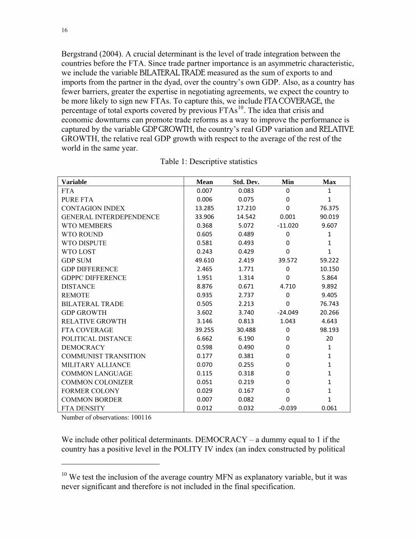
Bergstrand (2004). A crucial determinant is the level of trade integration between the countries before the FTA. Since trade partner importance is an asymmetric characteristic, we include the variable BILATERAL TRADE measured as the sum of exports to and imports from the partner in the dyad, over the country’s own GDP. Also, as a country has fewer barriers, greater the expertise in negotiating agreements, we expect the country to be more likely to sign new FTAs. To capture this, we include FTA COVERAGE, the percentage of total exports covered by previous FTAsF

10F. The idea that crisis and

economic downturns can promote trade reforms as a way to improve the performance is captured by the variable GDP GROWTH, the country’s real GDP variation and RELATIVE GROWTH, the relative real GDP growth with respect to the average of the rest of the world in the same year.

Table 1: Descriptive statistics

Variable Mean Std. Dev. Min Max FTA 0.007  0.083  0  1 PURE FTA 0.006  0.075  0  1 CONTAGION INDEX 13.285  17.210  0  76.375 GENERAL INTERDEPENDENCE 33.906  14.542  0.001  90.019 WTO MEMBERS 0.368  5.072  ‐11.020  9.607 WTO ROUND 0.605  0.489  0  1 WTO DISPUTE 0.581  0.493  0  1 WTO LOST 0.243  0.429  0  1 GDP SUM 49.610  2.419  39.572  59.222 GDP DIFFERENCE 2.465  1.771  0  10.150 GDPPC DIFFERENCE 1.951  1.314  0  5.864 DISTANCE 8.876  0.671  4.710  9.892 REMOTE 0.935  2.737  0  9.405 BILATERAL TRADE 0.505  2.213  0  76.743 GDP GROWTH 3.602  3.740  ‐24.049  20.266 RELATIVE GROWTH 3.146  0.813  1.043  4.643 FTA COVERAGE 39.255  30.488  0  98.193 POLITICAL DISTANCE 6.662  6.190  0  20 DEMOCRACY 0.598  0.490  0  1 COMMUNIST TRANSITION 0.177  0.381  0  1 MILITARY ALLIANCE 0.070  0.255  0  1 COMMON LANGUAGE 0.115  0.318  0  1 COMMON COLONIZER 0.051  0.219  0  1 FORMER COLONY 0.029  0.167  0  1 COMMON BORDER 0.007  0.082  0  1 FTA DENSITY 0.012  0.032  ‐0.039  0.061 Number of observations: 100116

We include other political determinants. DEMOCRACY – a dummy equal to 1 if the country has a positive level in the POLITY IV index (an index constructed by political

10 We test the inclusion of the average country MFN as explanatory variable, but it was never significant and therefore is not included in the final specification.

17

scientists that ranges from -10 to 10, increasing in democratic level). We also test the related idea that countries with political regimes that are more similar will be more likely to sign an agreement including the dyad-year level variable POLITICAL DISTANCE, namely the absolute difference in the POLITY IV values. The quest for geopolitical stability is captured by the variable MILITARY ALLIANCE, which is a dummy variable equal to 1 if the countries concerned are in a military alliance (we get this from the Correlates of War database). To control for the opening of Central and Eastern nations to the world trade system, another dummy, COMMUNIST TRANSITION, is unity if one of the countries is a former communist economy.

Some other country-pair common characteristics are included in the regressions but not reported for the sake of space: border, language, colonizer and former colonial relation. Also, we add a time trend and the (detrended) proportion of total dyads covered by FTAs in a given year.

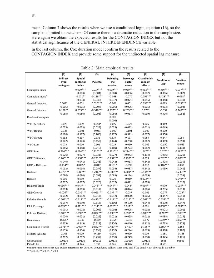
5.3. 17BEstimation Results The main results of the empirical exercises are in Table 2. The discussion begins with the first five rows of Table 2 that focus on different measures of spatial dependence and their respective quadratic terms.

In column 1, only the undirected spatial lag, GENERAL INTERDEPENDENCE, is included in the regression. Our results reproduce the finding of previous studies as the coefficient is positive and significant (but just at the 10% of confidence). In Column 2, we add the CONTAGION INDEX and see that this changes the results. The CONTAGION INDEX is positive and significant with less than a 1% probability of error, and its quadratic term is negative, indicating a threshold effect. Interestingly, the coefficient on the GENERAL INTERDEPENDENCE index becomes insignificant. In Column 3, we do the same test but use only agreements classified as ‘pure FTA’ in the Hufbauer and Schott (2009) database. The results hold for the CONTAGION INDEX, but the undirected spatial effect is again positive and significant.

In column 4 we use the broader definition of FTA as a dependent variable and seek to show that our results on the CONTAGION INDEX are not spurious. We create a “RANDOM CONTAGION INDEX” that is calculated in the same way as the CONTAGION INDEX, but using random exports and import shares. This variable is not significant, showing that the theoretically-justified weight matters – the positive influence of contagion does not depend merely on the use of directed versus undirected dyads.

Since the inference with dyadic data imposes additional complications, in Column 5 we reproduce the model of Column 2 but adjust the standard errors by two-ways clustering. Even the standard errors are now about the double of the previous size, the main conclusions are the same, apart from the fact that the quadratic term becomes insignificant even at the 10% level.

In Columns 6 and 7 we address the issue of unobservable heterogeneity. In column 6 we estimate a Chamberlain probit random effects model in which the averages of the time-varying regressors are added as controls (not displayed in the table). Some results change, notably the GENERAL INDEPENDENCE variable becomes negative. This is due to the fact that this index has little time variation and is thus highly correlated with its own

18

mean. Column 7 shows the results when we use a conditional logit, equation (16), so the sample is limited to switchers. Of course there is a dramatic reduction in the sample size. Here again we obtain the expected results for the CONTAGION INDEX but not the statistical significance of the GENERAL INTERDEPENDENCE variable.

In the last column, the Cox duration model confirm the results related to the CONTAGION INDEX and provide some support for the undirected spatial lag measure.

Table 2: Main empirical results    (1)  (2)  (3) (4) (5) (6) (7)  (8)

  Indirect dyad 

contagion 

Spatial contagion index 

Pure fta Defeating 

the random 

Two ways cluster errors 

Chamberlain random effects 

Conditional Logit 

Duration model 

Contagion Index

   0.020***  0.027*** 0.019*** 0.020*** 0.012***  0.356***  0.017***   (0.003)  (0.004) (0.004) (0.006) (0.002) (0.086)  (0.002)

Contagion Index2    ‐0.071**  ‐0.126*** ‐0.053 ‐0.070 ‐0.055***  ‐1.428***  ‐0.058*    (0.033)  (0.036) (0.037) (0.071) (0.015) (0.448)  (0.031)General Interdep. 0.009*  0.001  0.020*** ‐0.001 0.001 ‐0.036***  0.013  0.013*** (0.005)  (0.005)  (0.007) (0.005) (0.006) (0.005) (0.033)  (0.003)General Interdep.2 0.198**  0.239***  ‐0.348*** 0.237*** 0.239*** 0.076* ‐0.354  0.240*** (0.085)  (0.086)  (0.093) (0.086) (0.037) (0.039) (0.406)  (0.052)Random Contagion      0.001        (0.006)  WTO Members ‐0.025  ‐0.024  ‐0.048* ‐0.022 ‐0.023 0.006 0.019  (0.023)  (0.023)  (0.025) (0.023) (0.032) (0.011) (0.049) WTO Round ‐0.135  ‐0.101  ‐0.083 ‐0.099 ‐0.101 ‐0.109 0.100  (0.176)  (0.177)  (0.208) (0.177) (0.321) (0.077) (0.350) WTO dispute 0.192  0.197  0.135 0.179 0.197 0.084 0.247  0.055 (0.142)  (0.143)  (0.159) (0.144) (0.230) (0.062) (0.309)  (0.093)WTO Lost 0.073  0.010  0.101 0.019 0.010 ‐0.002 ‐0.150  ‐0.033 (0.185)  (0.188)  (0.210) (0.189) (0.273) (0.082) (0.467)  (0.139)GDP Sum 0.234***  0.224***  0.220*** 0.221*** 0.224*** 1.247***  10.07***  0.187*** (0.026)  (0.027)  (0.031) (0.027) (0.042) (0.114) (1.936)  (0.020)GDP Difference ‐0.240***  ‐0.232*** ‐0.231*** ‐0.232*** ‐0.232*** 0.019 6.232***  ‐0.200*** (0.040)  (0.041)  (0.048) (0.042) (0.057) (0.142) (1.628)  (0.030)GDPpc Difference ‐0.114**  ‐0.095*  ‐0.047 ‐0.101* ‐0.095 0.232 6.316***  ‐0.051 (0.052)  (0.054)  (0.057) (0.054) (0.087) (0.141) (2.039)  (0.041)Distance ‐1.376***  ‐1.30***  ‐1.216*** ‐1.305*** ‐1.301*** ‐0.544***    ‐1.249*** (0.080)  (0.084)  (0.092) (0.085) (0.124) (0.039)   (0.055)Remote 0.006  0.019  0.022 0.020 0.019 0.022***    0.049*** (0.017)  (0.017)  (0.020) (0.017) (0.021) (0.009)   (0.012)Bilateral Trade 0.036***  0.043***  0.046*** 0.044*** 0.043* 0.016***  0.070  0.035*** (0.013)  (0.013)  (0.017) (0.013) (0.024) (0.006) (0.235)  (0.013)GDP Growth ‐0.026**  ‐0.036*** ‐0.053*** ‐0.037*** ‐0.037 ‐0.005 ‐0.077  ‐0.023** (0.012)  (0.012)  (0.013) (0.012) (0.030) (0.005) (0.047)  (0.011)Relative Growth ‐0.604***  ‐0.612*** ‐0.475*** ‐0.617*** ‐0.612*** ‐0.261***  ‐0.533***  0.202 (0.097)  (0.099)  (0.116) (0.100) (0.190) (0.044) (0.170)  (1.247)FTA Coverage 0.009***  0.011***  0.014*** 0.012*** 0.011** 0.001 0.058***  0.009*** (0.001)  (0.002)  (0.002) (0.002) (0.005) (0.002) (0.021)  (0.001)Political Distance ‐0.105***  ‐0.099*** ‐0.092*** ‐0.099*** ‐0.099*** ‐0.100***  ‐0.212**  ‐0.103*** (0.020)  (0.021)  (0.025) (0.021) (0.025) (0.012) (0.088)  (0.015)Democracy ‐0.395*  ‐0.340  ‐0.439 ‐0.354 ‐0.340 ‐0.177 16.89***  ‐0.655*** (0.235)  (0.249)  (0.312) (0.250) (0.440) (0.112) (0.713)  (0.178)Communist Transit. ‐0.671***  ‐0.467*** ‐0.862*** ‐0.487*** ‐0.467* 0.165**  ‐5.100***  0.154 (0.155)  (0.156)  (0.158) (0.157) (0.274) (0.079) (0.968)  (0.102)Military Alliance ‐0.105  0.029  ‐0.119 0.030 0.029 0.009 1.181  ‐0.165 (0.212)  (0.217)  (0.237) (0.218) (0.249) (0.098) (0.925)  (0.126)Observations 100116  100116  100116 100116 100116 100116 3698  99809Pseudo R2 0.317  0.326  0.333 0.326 0.326 0.394 0.601 Standard errors clustered at dyad level in parentheses Six duration dependence splines, time trend and FTA density not showed in the table. . *** p<0.01, ** p<0.05, * p<0.1

19

Taken together, these results provide strong support for the notion that FTAs are contagious when this effect is measured by our theoretically motivated contagion index. It also supports the idea of decreasing marginal effects of this contagion effect, captured by the quadratic term. By contrast, we find that the undirected measure of spatial dependence (GENERAL INTERDEPENDENCE) is not robust to the different specifications.

In addition, with respect to other hypothesis of the FTA formation, we find little evidence that developments at the multilateral level have an impact. The four variables from the Mansfield and Reinhardt (2003) study are almost always insignificant and often with unexpected signs. Also, we find weak support for the idea that democracy influence regionalism, since DEMOCRACY has the wrong sign and is statistically insignificant, with the interesting exception of the conditional logit estimates. Nevertheless, the similarity of political regimes seems to have an effect as POLITICAL DISTANCE is always negative and significant, indicating that very different political regimes have trouble signing agreements. In terms of the integration of the Eastern bloc hypothesis, the variable COMMUNIST TRANSITION has a negative sign, providing no support for the idea; this result should be interpreted with caution since several of the former communist countries are excluded from our sample due to a lack of data. The other political variable, MILITARY ALLIANCE is never significant.

All the economic and geographical determinants have the expected sign and significance. In terms of the dyad level DISTANCE, GDP DIFFERENCE and GDPPC DIFFERENCE are always negative and significant (except in the conditional logit for the last two), the opposite for REMOTE and GDP SUM. For the country level variables, BILATERAL TRADE indicates that previous trade level with the partner is a significant predictor of FTAs. Also, the more FTAs a country has, the more likely it will continue with others, since the variable FTA COVERAGE is also positive and significant. The variables GDP GROWTH and RELATIVE GROWTH are both negative and significant, providing some preliminary evidence to the idea that trade reforms are more likely in economic downturns.

5.4. 18BQuantification of the results The nature of our empirical strategy makes quantification a difficult task. The dependent variable is a switch from non-FTA status to FTA status – a rare event in our data set, just 0.7% of the observations classified as non-zeros for all type of agreements and 0.6% for pure agreements (Table 1). This implies that the traditional “correct classification ratio” that assigns a value 1 to all predicted values over 0.5 and zero otherwise is uninformative in our case. An alternative is to use the sample mean of the dependent variable as a cut-off when classifying correctly predicted values. If we do so, we find that the model in column 1 of Table 2 correctly predicts 85.5% of the cases, while the model in column 2, that includes the contagion index, correctly predicts 84.5% of the non-zeros.

One different way to quantify the results is to take advantage of the fact that logit estimates can be interpreted in terms of changes in the odds. Specifically, we calculate the change in the odds-ratio of one standard deviation increase in the regressor keeping all the other variables constant. The results for the model using all type of agreements and

20

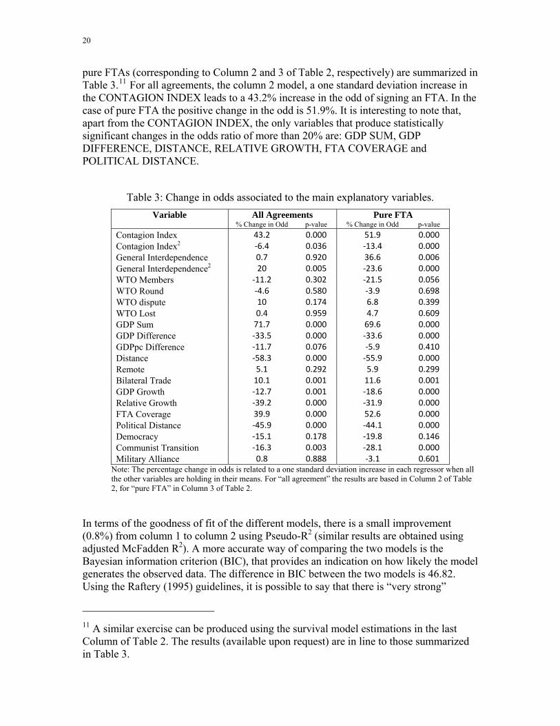
pure FTAs (corresponding to Column 2 and 3 of Table 2, respectively) are summarized in Table 3.F

11F For all agreements, the column 2 model, a one standard deviation increase in

the CONTAGION INDEX leads to a 43.2% increase in the odd of signing an FTA. In the case of pure FTA the positive change in the odd is 51.9%. It is interesting to note that, apart from the CONTAGION INDEX, the only variables that produce statistically significant changes in the odds ratio of more than 20% are: GDP SUM, GDP DIFFERENCE, DISTANCE, RELATIVE GROWTH, FTA COVERAGE and POLITICAL DISTANCE.

Table 3: Change in odds associated to the main explanatory variables. Variable All Agreements Pure FTA

% Change in Odd p-value % Change in Odd p-value Contagion Index 43.2 0.000 51.9 0.000 Contagion Index2 ‐6.4 0.036 ‐13.4 0.000 General Interdependence 0.7 0.920 36.6 0.006 General Interdependence2 20 0.005 ‐23.6 0.000 WTO Members ‐11.2 0.302 ‐21.5 0.056 WTO Round ‐4.6 0.580 ‐3.9 0.698 WTO dispute 10 0.174 6.8 0.399 WTO Lost 0.4 0.959 4.7 0.609 GDP Sum 71.7 0.000 69.6 0.000 GDP Difference ‐33.5 0.000 ‐33.6 0.000 GDPpc Difference ‐11.7 0.076 ‐5.9 0.410 Distance ‐58.3 0.000 ‐55.9 0.000 Remote 5.1 0.292 5.9 0.299 Bilateral Trade 10.1 0.001 11.6 0.001 GDP Growth ‐12.7 0.001 ‐18.6 0.000 Relative Growth ‐39.2 0.000 ‐31.9 0.000 FTA Coverage 39.9 0.000 52.6 0.000 Political Distance ‐45.9 0.000 ‐44.1 0.000 Democracy ‐15.1 0.178 ‐19.8 0.146 Communist Transition ‐16.3 0.003 ‐28.1 0.000 Military Alliance 0.8 0.888 ‐3.1 0.601 

Note: The percentage change in odds is related to a one standard deviation increase in each regressor when all the other variables are holding in their means. For “all agreement” the results are based in Column 2 of Table 2, for “pure FTA” in Column 3 of Table 2.

In terms of the goodness of fit of the different models, there is a small improvement (0.8%) from column 1 to column 2 using Pseudo-R2 (similar results are obtained using adjusted McFadden R2). A more accurate way of comparing the two models is the Bayesian information criterion (BIC), that provides an indication on how likely the model generates the observed data. The difference in BIC between the two models is 46.82. Using the Raftery (1995) guidelines, it is possible to say that there is “very strong”

11 A similar exercise can be produced using the survival model estimations in the last Column of Table 2. The results (available upon request) are in line to those summarized in Table 3.

21

support for the use of the contagion index. The Akaike’s information criteria (AIC), with a decrease of 65.92 in the model that includes the contagion index, support this conclusion. For all other specifications, the information measures yield similar results. In the model for pure FTA, the difference in BIC is 10.51, while in the conditional logit it is 35.08.

6. 5BCONCLUDING REMARKS The rapid proliferation of FTAs is one of the more remarkable developments of the world trade system over the past decades. As it involves more than a hundred nations and many different types of agreements, the driving force behind this trend is surely quite complex. Our paper is an effort to understand the theoretical and empirical determinants of this proliferation.

Our basic theoretical hypothesis is that much of the spread of regionalism is driven by a domino-like effect whereby FTAs between a nation’s trade partners rearranges the array of political economy forces in such as way as to make the nation more likely to sign an FTA. Putting it roughly, FTAs are contagious and the degree of contagion is related to the importance of the partners’ markets.

We believe our paper contains three elements of value-added. First it extends the Baldwin (1993) domino theory of regionalism to allow for FTAs (the original paper applied only to customs unions). Second, we use this model to develop a theory-based directed measure of contagion. Third, we use this measure, the ‘contagion index’, to test for domino effects and to test these against alternative hypotheses. Our main finding is that the contagion phenomenon is present in our data and robust to various econometric specifications and samples, including allowing for other effects (e.g. the bandwagon effect, slow-multilateralism, etc.).

6BREFERENCES Aghion, Philippe, Pol Antràs and Elhanan Helpman (2007). "Negotiating free trade," Journal of International Economics, vol. 73(1), pages 1-30.

Baier, Scott and Jeffrey Bergstrand (2004). “Economic Determinants of Free Trade Agreements”. Journal of International Economics, vol. 64, pp. 29-63.

Baldwin, Richard (1993). “A domino theory of regionalism,” NBER WP 4465. Eventually published in Baldwin, Haaparanta and Kiander (eds.), Expanding membership of the European Union, Cambridge University Press, 1995.

Baldwin, Richard (1994). Towards an integrated Europe, CEPR, London.

Baldwin, Richard (1997). “The causes of regionalism,” The World Economy, Vol. 20, No, 7, pp 865-888.

Baldwin, Richard (1999). “Agglomeration and endogenous capital,” European Economic Review 43, 253-280.

Baldwin, Richard (2008). “Managing the Noodle Bowl: The fragility of East Asian Regionalism,” Singapore Economic Review, vol. 53, issue 03, pages 449-478.

22

Baldwin, Richard, Rikard Forslid, Philippe Martin, Gianmarco Ottaviano, and Frederic Robert-Nicoud (2003). Economic Geography and Public Policy, Princeton University Press.

Baldwin, Richard and Roland Rieder (2007). “A test of endogenous trade bloc formation theory on EU data,” Journal of International Economic Studies, 11(2), pp 77–111.

Baldwin, Richard and Frédéric Robert-Nicoud (2007). “HEntry and Asymmetric Lobbying: Why Governments Pick LosersH,” HJournal of the European Economic AssociationH, MIT Press, vol. 5(5), pages 1064-1093, 09.

Beck, Nathaniel, Jonathan Katz, and Richard Tucker (1998). “Taking Time Seriously: Time-Series–Cross-Section Analysis with a Binary Dependent Variable”. American Journal of Political Science. Vol. 42, No. 4, pp. 1260-1288.

Bhagwati, Jagdish (1991). The World Trading System at Risk, Princeton University Press, Princeton, New Jersey:

Bhagwati, Jagdish (1993). “Regionalism and multilateralism: An overview,” in Anderson, K and Blackhurst, R. (eds), Regional integration and the global trading system, (London: Harvester-Wheatsheaf).

Bhagwati, Jagdish (2008). Termites in the Trading System: How Preferential Agreements Undermine Free Trade. Oxford University Press.

Cameron, C., J. Gelbach, and D. Miller (2009). “Robust Inference with Multi-way Clustering”. University of California at Davis, Department of Economics. Working Paper 09-9.

Chamberlain, Gary (1980). “Analysis of Covariance with Qualitative Data,” Review of Economic Studies, Vol. XLVII(1), No. 146.

Corden, W. M. (1974). Trade Policy and Economic Welfare, Oxford: Clarendon Press.

Egger, Peter and Mario Larch, “Interdependent Preferential Trade Agreement Memberships: An Empirical Analysis,” Journal of International Economics 76 (2), 2008, 384–399.

Marcel Fafchamps & Flore Gubert, 2007. “HRisk Sharing and Network FormationH,” HAmerican Economic ReviewH, vol. 97(2), pages 75-79.

Freund, Caroline (2000). “Different Paths to Free Trade: The Gains from Regionalism”, Quarterly Journal of Economics 115:4, 1317-1341.

Grossman, G. and E. Helpman (1994). “Protection for Sale” The American Economic Review, Vol. 84, No. 4, 833-850.

Harvie, Charles, Fukunari Kimura, Hyun-Hoon Lee, eds (2006). New East Asian Regionalism: Causes, Progress And Country Perspectives, Edward Elgar Publishing.

Holmes, Tammy (2005). “What Drives Regional Trade Agreements that Work?” HEI Working Paper, No. 07/2005, Graduate Institute of International Studies, Geneva.

Hufbauer, G. (1989). Background Paper for The Free Trade Debate, Reports of the 20th Century Fund Task Force on the Future of American Trade Policy, Priority Press, New York.

23

Hufbauer, G. and J. Schott (2009). “Fitting Asia-Pacific agreements into the WTO system,” in R. Baldwin and P. Low (eds), Multilateralising Regionalism: Challenges for the global trading system, Cambridge University Press.

Jaimovich, Dany (2010). “A Bayesian spatial probit estimation of the Contagion Index in Free Trade Agreements”, HEID working papers, Graduate Institute of International Studies, Geneva.

King, Gary, and Langche Zeng (2001). Explaining Rare Events in International Relations. International Organization, 55, 3: 693-715.

Krishna, Pravind (1998). “Regionalism and Multilateralism: A Political Economy Approach,” Quarterly Journal of Economics, February 1998, Vol. 113, No. 1, Pages 227-250.

Krugman, Paul (1991). "The move toward free trade zones," Economic Review, Federal Reserve Bank of Kansas City, issue Nov, pages 5-25.

Krugman, Paul (1993). “Regionalism versus multilateralism: Analytic notes”, in De Melo, J. and Panagariya, A. (eds), New dimensions in regional integration, (Cambridge: Cambridge University Press for CEPR).

Lawrence, R. (1996). Regionalism, multilateralism and deeper integration, Brookings Institute, Washington.

Lester, Simon and Bryan Mercurio, eds (2009). Bilateral and Regional Trade Agreements: Commentary and Analysis, Cambridge University Press, Cambridge.

Manger, Mark (2006). “The Political Economy of Discrimination: Modelling the Spread of Preferential Trade Agreements”. Working Paper. Montreal, Department of Political Science, McGill University.

Mansfield, E.D. and E. Reinhardt (2003). “Multilateral Determinants of Regionalism: The Effects of GATT/WTO on the Formation of Preferential Trade Agreements,” International Organization, vol. 57, pp. 829-862. Mansfield, Edward, Helen Milner and B. Peter Rosendorff (2002). “Replication, Realism, and Robustness: Analyzing Political Regimes and International Trade,” American Political Science Review, 96(1):167-69.

Mansfield, Edward and Jon Pevehouse (2000). “Trade Blocs, Trade Flows, and International Conflict” International Organization, Vol. 54, No. 4, pp. 775-808.

Martin, Philippe, Thierry Mayer and Mathias Thoenig (2008) “Make Trade not War?” Review of Economic Studies, 2008, vol. 75(3).

Martin, Philippe, Thierry Mayer and Mathias Thoenig (2010). "The geography of conflicts and free trade agreements", CEPR Discussion Paper 7740.

Neumayer, Eric and Thomas Plumper (2010). “Spatial Effects in Dyadic Data”. International Organization, 64 : 145-166.

Raftery, A.E. (1995). “HBayesian model selection in social research”.H Sociological Methodology, 25, 111-196.

24

Riezman, Raymond (1985). “Customs unions and the core”, Journal of International Economics, vol. 19(3-4), pp 355-365.

Sapir, A. (1997).”Domino effects in Western European Trade, 1960-1992,” CEPR DP 1576, published in European Journal of Political Economy, Vol 17: 386, 2001.

Solis, M., B. Stallings, S. Katada (2009). Competitive Regionalism: FTAs in the Pacific Rim, Palgrace, MacMillan, New York.

Vicard, Vincent (2008). “Trade, conflicts and political integration: explaining the heterogeneity of regional trade agreements”. Documents de travail du Centre d'Economie de la Sorbonne.

Whalley, J. (1993). “Regional trade arrangements in North America: CUSTA and NAFTA,” in De Melo, J. and Panagariya, A. (eds), New dimensions in regional integration, Cambridge University Press, Cambridge

Wooldridge, J. (2002) “Econometric analysis of cross section and panel data”, MIT Press.

Wu, J.P. (2004). “Measuring and Explaining Levels of Regional Economic Integration,” ZEI Working Paper B12/2004, Centre for European Integration Studies, Bonn.

Yi, S. (1996). “Endogenous formation of customs unions under imperfect competition: Open regionalism is good,” Journal of International Economics, 41, 151-175.

25

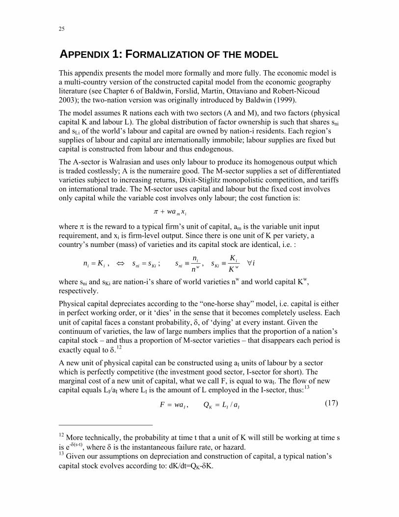
7BAPPENDIX 1: FORMALIZATION OF THE MODEL This appendix presents the model more formally and more fully. The economic model is a multi-country version of the constructed capital model from the economic geography literature (see Chapter 6 of Baldwin, Forslid, Martin, Ottaviano and Robert-Nicoud 2003); the two-nation version was originally introduced by Baldwin (1999).

The model assumes R nations each with two sectors (A and M), and two factors (physical capital K and labour L). The global distribution of factor ownership is such that shares sni and sLi of the world’s labour and capital are owned by nation-i residents. Each region’s supplies of labour and capital are internationally immobile; labour supplies are fixed but capital is constructed from labour and thus endogenous.

The A-sector is Walrasian and uses only labour to produce its homogenous output which is traded costlessly; A is the numeraire good. The M-sector supplies a set of differentiated varieties subject to increasing returns, Dixit-Stiglitz monopolistic competition, and tariffs on international trade. The M-sector uses capital and labour but the fixed cost involves only capital while the variable cost involves only labour; the cost function is: im xwa+π

where π is the reward to a typical firm’s unit of capital, am is the variable unit input requirement, and xi is firm-level output. Since there is one unit of K per variety, a country’s number (mass) of varieties and its capital stock are identical, i.e. :

iKK

snn

sssKn wi

Kiwi

niKiniii ∀≡≡=⇔= ,;,

IIKI aLQwaF /,

where sni and sKi are nation-i’s share of world varieties nw and world capital Kw, respectively.

Physical capital depreciates according to the “one-horse shay” model, i.e. capital is either in perfect working order, or it ‘dies’ in the sense that it becomes completely useless. Each unit of capital faces a constant probability, δ, of ‘dying’ at every instant. Given the continuum of varieties, the law of large numbers implies that the proportion of a nation’s capital stock – and thus a proportion of M-sector varieties – that disappears each period is exactly equal to δ.F

12F

A new unit of physical capital can be constructed using aI units of labour by a sector which is perfectly competitive (the investment good sector, I-sector for short). The marginal cost of a new unit of capital, what we call F, is equal to waI. The flow of new capital equals LI/aI where LI is the amount of L employed in the I-sector, thus:F

13

== (17)

12 More technically, the probability at time t that a unit of K will still be working at time s is e-δ(s-t), where δ is the instantaneous failure rate, or hazard. 13 Given our assumptions on depreciation and construction of capital, a typical nation’s capital stock evolves according to: dK/dt=QK-δK.

26

where QK is the I-sector’s output, i.e. the flow of newly constructed capital.

Instantaneous preferences over A and M goods are given by:

σμσμμ <<<⎟⎠⎞⎜

⎝⎛≡≡= ∫ Γ∈

−− 10,,; /111

i iMAM dicC CCCCUσ )/(1 1/-1

∞− tρ

AA pE /)1(

(18)

Since capital is constructed, intertemporal issues are unavoidable; the assumed intertemporal preferences are:

ln

0∫=

=t

CdteU

(19)

where ρ is the subjective discount rate.

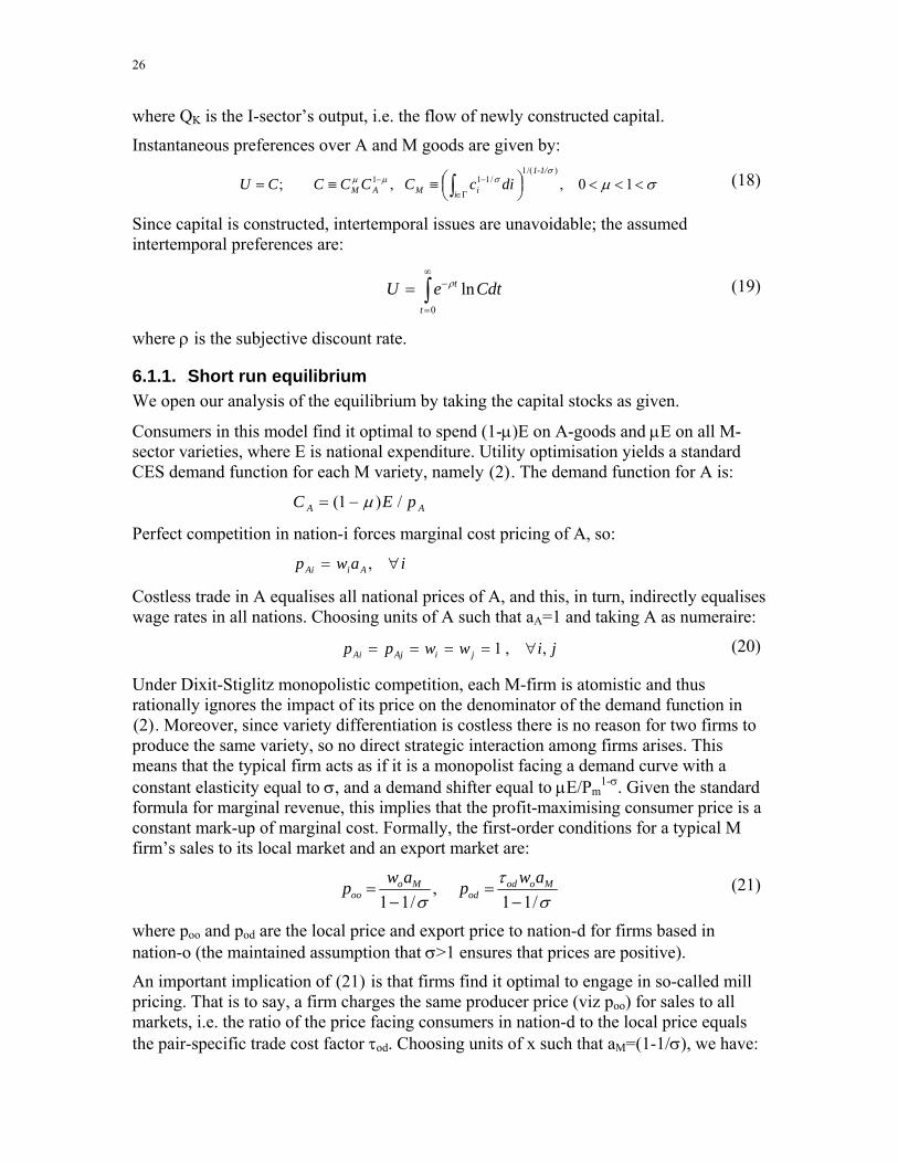
6.1.1. 23BShort run equilibrium We open our analysis of the equilibrium by taking the capital stocks as given.

Consumers in this model find it optimal to spend (1-μ)E on A-goods and μE on all M-sector varieties, where E is national expenditure. Utility optimisation yields a standard CES demand function for each M variety, namely X(2)X. The demand function for A is:

C μ−=

Perfect competition in nation-i forces marginal cost pricing of A, so: iawp AiAi ∀= ,

Costless trade in A equalises all national prices of A, and this, in turn, indirectly equalises wage rates in all nations. Choosing units of A such that aA=1 and taking A as numeraire:

(20)pp AjAi jiww ji ,,1= = = = ∀

Under Dixit-Stiglitz monopolistic competition, each M-firm is atomistic and thus rationally ignores the impact of its price on the denominator of the demand function in X(2)X. Moreover, since variety differentiation is costless there is no reason for two firms to produce the same variety, so no direct strategic interaction among firms arises. This means that the typical firm acts as if it is a monopolist facing a demand curve with a constant elasticity equal to σ, and a demand shifter equal to μE/Pm

1-σ. Given the standard formula for marginal revenue, this implies that the profit-maximising consumer price is a constant mark-up of marginal cost. Formally, the first-order conditions for a typical M firm’s sales to its local market and an export market are:

τσσ /11

,/11 −

=−

= Moodod

Mooo

aw p aw p (21)

where poo and pod are the local price and export price to nation-d for firms based in nation-o (the maintained assumption that σ>1 ensures that prices are positive). An important implication of X(21)X is that firms find it optimal to engage in so-called mill pricing. That is to say, a firm charges the same producer price (viz poo) for sales to all markets, i.e. the ratio of the price facing consumers in nation-d to the local price equals the pair-specific trade cost factor τod. Choosing units of x such that aM=(1-1/σ), we have:

27

,,1 ododoo p p τ== (22)

Mill pricing makes it very easy to calculate the equilibrium operating profit earned by a typical firm in any market. By definition, πod=(pod -mcod)xod and since pod=mcod(1-1/σ), we have πod=pod xod/σ. Thus, using X(2)X and the fact that all firms engage in mill pricing, operating profit for a typical firm is:

σμπ ≡= b

KEbD w

w

ood ; (23)

where b is defined for notational convenience, and Do is the effective demand facing a typical firm in nation-o, namely:

∑∑ ===Δ≡

Δ≡≡

R

d niiddwd

Edd

Edd

R

d dod sE

sBBD11o ,,, φφ

Es

Here φod≡τod1-σ is our measure of bilateral trade freeness, the B’s are the market specific

demand shifters, sEi is nation-i's share of world expenditure, and

6.1.2. 24BThe Market Size Condition As X(23)X shows, capital’s reward depends upon the spatial distribution of industry (the sni’s) and the spatial distribution of expenditure (the sEi’s). Since capital’s reward is the fulcrum of our analysis and we are taking sn as given for the moment, the next task is to characterise the sEi’s. We begin with the denominator, Ew.

Capital construction uses resources, so consumption expenditure does not equal income in this model. At the world level, consumption expenditure equals world income minus world spending on new capital. World income is the wage bill plus operating profits, i.e. Lw+bEw.F

14F Spending on capital construction equals the value of resources employed by I-

sectors, which we denote as LIw.F

15F Given X(17)X, the amount of labour necessary to

maintain the world capital stock equals δaIKw. Using this and the definition Ew= Lw+bEw-LI

w:

bKaLE

wI

ww

−−

=1δ

(24)

where Kw is the worldwide capital stock (to be determined below).

To finish our characterisation of sEi, we calculate expenditure of typical nation-i. The nation’s income comprises its labour income, sLiLw, (where sLi is its share of world labour), its capital income is bsniDiEw. From this, we subtract its share of world depreciation, namely sniδKw. Thus Ei=sLiLw+bsniDiEw-sniδaIKw. Taking the ratio of this to our expression for world expenditure:

14 With mill pricing, operating profit is 1/σ times sales and μEw is world-wide sales. 15 Spending on capital accumulation equals the I-sector total cost since, by perfect competition, its revenue always equals its total costs.

28

oniw

Iw

wIni

wLi

E DbsKaL

KasLsbs +

−−

−=δδ

)1( (25)

6.1.3. 25BLong Run Equilibrium In the long run, national capital stocks are endogenous and rise or fall until the cost of constructing/replacing a new unit of capital just equals the present value of the income stream it would generate. Finding the long-run equilibrium capital stocks requires evaluation of the costs and benefits of having an extra unit of capital.

In any interior long-run equilibrium (i.e. where 0<sni<1 for all i), all nations must be actively constructing enough capital to replace depreciation and the value of extra capital created must equal its construction cost F. To summarise:

10..; ∀ < ≤= nii stsiFv

δρ −−= rEE /&

(26)

where v denotes the present value of a unit of capital, and F=aI is the construction cost for a unit of capital.

To finish our characterisation of the long run we need to find the v’s. This is where intertemporal features enter the model. The classic way of expressing optimal intertemporal consumption behaviour with respect to X(19)X is the so-called Euler equation:

This can be easily derived using the Hamiltonian approach to maximising X(19)X, noting that each unit of capital has a probability of being ‘alive’ at time t equal to e-δt. The only aspect of this intertemporal optimisation affects the calculations is the fact that in the long-run equilibrium, E stops evolving, so r=ρ+δ. Using this to calculate the present value of a unit of capital in nation-i:

iv ii ∀

+= ;

δρπ

(27)

6.1.4. 26BCharacterising the Long Run Equilibria We turn next to finding Kw. From X(26)X and X(27)X, π’s are equalised, so each unit of capital must earn the world average reward, namely bEw divided by Kw. From X(26)X and X(17)X, (bEw/Kw) must equal aI(ρ+δ), so Kw=bEw/[(ρ+δ)aI]. Solving this together with X(24)X, the long-run equilibrium values of Ew and Kw are:

δρ

ρββρβ

β+

≡−

=−

=bLE

aLK

ww

I

ww ;

1,

)1( (28)

where β is a group of parameters that frequently appears. Using these, in X(25)X, we have: (29)

LiniEi sss )1( ββ −+=

so a nation’s share of world expenditure is its weighted average of its share of Lw and Kw.

29

The equalisation of the π’s implied by X(26)X and X(27)X, pins down the equilibrium location of industry among all nations, i.e. the sni’s. From X(23)X, the sni’s, enter in the denominator of in the B’s, so the resulting system of equation is non-linear and we cannot find general solutions.

One special case that does allow solution is that of symmetric MFN tariffs. In this case we can solve X(26)X to find that the equilibrium distribution of industry is:F

16

i

RsR

Rs Eini ∀−⎟⎟

⎠

⎞⎜⎜⎝

⎛−

++= ),1(1

11φ

φ (30)

Assuming the distribution of expenditure is sufficiently even to ensure all the sni’s are positive. This tells that a nation’s share of industry deviates from the symmetric solution 1/R according to the region’s own size bias, i.e. the difference between its expenditure share and the even share 1/R.

6.2. 19BExplicit solutions for the R=3 case The example in the text relied on the case of R=3 when the nations were symmetric in their labour endowments, and initially symmetric in the MFN tariffs.

The text referred the reader to the Appendix on a number of points. The first was the assertion that allowing entry in nations 2 and 3 did not qualitatively change the impact on π1 in the case of an FTA between 2 and 3. When 2 and 3 form an FTA, the operating profit of a typical firm in either nation is:

2122113212 2,2,)( nnnnw

w

ssssBBBnEb +=Δ+=Δ++= φφφπ (31)

where by symmetry π3 is the same, and sn2=sn3. In the text, we normalised sn1=1/3 and so we impose that here following the logic that firms under profit pressure exit only slowly. Plugging all this into in X(30)X yields a quadratic equation in sn2. Solving the results is:

φφφφφφφ

12122713 4322

2+++−+−−

=ns

By inspection this exceeds 1/3 since 0≤φ≤1, thus as claimed in the text, the FTA between 2 and 3 leads to entry in those nations. This new entry alters the operating profit for nation 1 firms. In this case, nation-1 operating profit is:

31,)

22

2( 1121

21

2

21

11 ===

++

+= nEE

nn

E

nn

Ew

w

sssss

sss

snEb

φφ

φπ

16 The equality of π’s implies all the D’s from (23) must equal unity, and also that all the B’s must be equal. Adding up all the 1=Di equations yields R=(1+ (R-1)φ)RB. Since all the φs are the same, each Δ equals sni+φ(1-sni); using this in the B and solving yields the result.

30

By inspection, we can see that a rise in sn2 from 1/3 will lower π1. More precisely, plugging in the new equilibrium value of sn2 we have π1 equals:

This confirms the claim in the text that considering the full impact on π1 does not change the analysis qualititatively.

The second point concerned the assertion that an FTA between nations 1 and 2 when there was also an FTA between 2 and 3 would result in a π1 that was below its equilibrium value. This is a simple calculation since we investigate what happens to π1=π3 and π2, when all the n’s stay at 1/3. The operating profit for the ‘hub’ nation, nation-2, is:

)31

21(,)

31

22( 312 +

++

==++

=φφππ

φπ w

w

w

w

nEb

nEb

By inspection, the first expression is more than bEw/nw and the second is less, since φ<1.

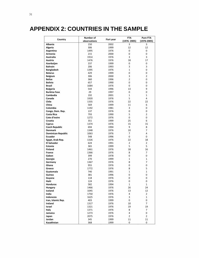
31

8BAPPENDIX 2: COUNTRIES IN THE SAMPLE

Country Number of observations 

Fisrt year FTA  

(1976‐ 2005) Pure FTA 

(1976‐2005) Albania  150 2002 3 3 Algeria  306 1999 12 12 Argentina  1495 1976 0 0 Armenia  215 2000 0 0 Australia  1914 1976 3 3 Austria  1476 1976 18 17 Azerbaijan  237 1999 0 0 Bahrain  206 1993 3 3 Bangladesh  1395 1976 1 0 Belarus  429 1999 0 0 Belgium  306 2000 3 2 Belize  360 1996 2 0 Bolivia  657 1990 0 0 Brazil  1684 1976 0 0 Bulgaria  544 1996 13 9 Burkina Faso 29 1997 0 0 Cambodia  192 2001 1 1 Canada  1920 1976 5 4 Chile  1335 1976 22 22 China  569 1999 11 6 Colombia  1192 1981 3 0 Congo, Dem. Rep.  137 1976 0 0 Costa Rica  793 1990 5 2 Cote d'Ivoire 1272 1976 0 0 Croatia  351 1999 25 6 Cyprus  1374 1976 15 15 Czech Republic  694 1994 9 8 Denmark  1348 1976 10 7 Dominican Republic  1063 1976 7 4 Ecuador  548 1996 0 0 Egypt, Arab Rep.  1326 1976 22 18 El Salvador  624 1991 2 2 Estonia  365 1999 5 5 Finland  1461 1976 18 16 France  1366 1976 8 7 Gabon  399 1978 0 0 Georgia  270 1999 1 1 Germany  1367 1976 8 7 Ghana  955 1976 0 0 Greece  1772 1976 8 5 Guatemala  740 1991 1 1 Guinea  381 1996 0 0 Guyana  118 1976 0 0 Haiti  124 1976 0 0 Honduras  582 1994 1 1 Hungary  1466 1976 26 24 Iceland  1045 1976 13 12 India  1750 1976 4 2 Indonesia  1625 1976 3 1 Iran, Islamic Rep.  403 1999 0 0 Ireland  1317 1976 10 7 Israel  1321 1976 19 19 Italy  1371 1976 8 7 Jamaica  1273 1976 4 0 Japan  2075 1976 2 2 Jordan  345 1999 11 11 Kazakhstan  368 1999 0 0 

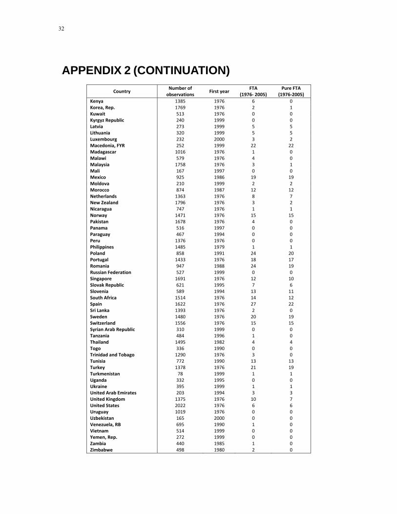
32

9BAPPENDIX 2 (CONTINUATION) Country 

Number of observations 

First year FTA  

(1976‐ 2005) Pure FTA 

(1976‐2005) Kenya  1385 1976 6 0 Korea, Rep.  1769 1976 2 1 Kuwait  513 1976 0 0 Kyrgyz Republic  240 1999 0 0 Latvia  273 1999 5 5 Lithuania  320 1999 5 5 Luxembourg  232 2000 3 2 Macedonia, FYR  252 1999 22 22 Madagascar  1016 1976 1 0 Malawi  579 1976 4 0 Malaysia  1758 1976 3 1 Mali  167 1997 0 0 Mexico  925 1986 19 19 Moldova  210 1999 2 2 Morocco  874 1987 12 12 Netherlands  1363 1976 8 7 New Zealand  1796 1976 3 2 Nicaragua  747 1976 1 1 Norway  1471 1976 15 15 Pakistan  1678 1976 4 0 Panama  516 1997 0 0 Paraguay  467 1994 0 0 Peru  1376 1976 0 0 Philippines  1485 1979 1 1 Poland  858 1991 24 20 Portugal  1433 1976 18 17 Romania  947 1988 24 19 Russian Federation  527 1999 0 0 Singapore  1691 1976 12 10 Slovak Republic  621 1995 7 6 Slovenia  589 1994 13 11 South Africa  1514 1976 14 12 Spain  1622 1976 27 22 Sri Lanka  1393 1976 2 0 Sweden  1480 1976 20 19 Switzerland  1556 1976 15 15 Syrian Arab Republic  310 1999 0 0 Tanzania  484 1996 1 0 Thailand  1495 1982 4 4 Togo  336 1990 0 0 Trinidad and Tobago  1290 1976 3 0 Tunisia  772 1990 13 13 Turkey  1378 1976 21 19 Turkmenistan  78 1999 1 1 Uganda  332 1995 0 0 Ukraine  395 1999 1 1 United Arab Emirates  203 1994 3 3 United Kingdom  1375 1976 10 7 United States 2022 1976 6 6 Uruguay  1019 1976 0 0 Uzbekistan  165 2000 0 0 Venezuela, RB  695 1990 1 0 Vietnam  514 1999 0 0 Yemen, Rep.  272 1999 0 0 Zambia  440 1985 1 0 Zimbabwe  498 1980 2 0 

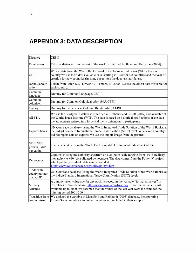
33

10BAPPENDIX 3: DATA DESCRIPTION

Distance CEPII

Remoteness Relative distance from the rest of the world, as defined by Baier and Bergstran (2004) :

GDP We use data from the World Bank's World Development Indicators (WDI). For each country we use the oldest available data, starting in 1960 for old countries and the year of creation for new countries (in some exceptions the data just start later).

capital/labour ratio

Taken from Baier, S.L., Dwyer, G., Tamura, R., 2000. We use the oldest data available for each country.

Common language Dummy for Common Language, CEPII.

Common colonizer Dummy for Common Colonizer after 1945, CEPII.

Colony Dummy for pairs ever in Colonial Relationship, CEPII.

All FTA We use the newly built database described in Hufbauer and Schott (2009) and available at the World Trade Institute (WTI). The data is based on historical notifications of the date the agreements entered into force and their contemporary participants.

Export Shares UN Comtrade database (using the World Integrated Trade Solution of the World Bank), at the 1-digit Standard International Trade Classification (SITC) level. Whenever a country did not report data on exports, we use the import image from the partner.

GDP, GDP growth, GDP per capita

The data is taken from the World Bank's World Development Indicators (WDI).

Democracy

Captures this regime authority spectrum on a 21-point scale ranging from -10 (hereditary monarchy) to +10 (consolidated democracy). The data comes from the Polity IV project, which publicly available data can be found at Hhttp://www.systemicpeace.org/polity/polity4.htmH

Trade with county partner over GDP

UN Comtrade database (using the World Integrated Trade Solution of the World Bank), at the 1-digit Standard International Trade Classification (SITC) level.

Military Alliance

A dummy taken value one for any positive record in the variable “formal alliances” in Correlates of War database: Hhttp://www.correlatesofwar.orgH Since the variable is just available up to 2000, we assumed that the values of the last year were the same for the missing period 2001-2004.

Transition from communism

We updated the variable in Mansfield and Reinhardt (2003) database, incorporating former Soviet republics and other countries not included in their sample.