1

Are Consumers in Developing Countries Willing-to-Pay More for Micronutrient-Dense Biofortified Foods? Evidence from a Field Experiment in Uganda1

Shyamal Chowdhury, University of Sydney2 J V Meenakshi, Delhi School of Economics

Keith Tomlins, University of Greenwich Constance Owori, Kawanda Agricultural Research Institute

Contributed Paper prepared for presentation at the International Association of Agricultural Economists Conference, Beijing, China, August 16-22, 2009

Copyright 2009 by S Chowdhury, JV Meenakshi, K Tomlins, C Owori. All rights reserved. Readers may make verbatim copies of this document for non-commercial purposes by any means, provided that this copyright notice appears on all such copies.

Abstract: Vitamin A deficiency is a major health problem in Africa and in many other developing countries. Biofortified staple crops that are high in pro vitamins A and adapted to local growing environment have the potential to reduce the prevalence of vitamin A deficiency. One such example is the orange-fleshed sweetpotato. However because of its distinctive orange color, which is in contrast to the white varieties that are typically consumed in Africa, it is important to assess whether consumers will accept it. It is this question that this paper attempts to address, using a choice experiment with the real product to quantify the magnitude of the premium or discount in consumers’ willingness to pay that may be associated with it. In addition, it also considers the extent to which the provision of nutrition information affects valuations. Finally, it addresses whether the use of hypothetical scenarios, both with and without a cheap talk script is justified in a developing country context, and quantifies the magnitude of hypothetical bias that results as a consequence. The experiment was conducted in Uganda, which is a key target country for the dissemination of orange-fleshed sweetpotato. Our results suggest that in the absence of nutrition information, there is no difference in the willingness to pay between white and orange varieties, but there is a discount for yellow sweetpotato (which does not have any beta-carotene). The provision of nutrition information does translate into substantial premia for the orange varieties, indicating that an information campaign may be key to drive market acceptance of the new product. Finally, there is a substantial hypothetical bias in both the WTP and the marginal WTP for the new varieties, and while cheap talk mitigates this bias, it does not eliminate it. Keywords: Cheap talk, Field experiments, Hypothetical bias, Conjoint analysis, Universal logit JEL classifications: C35, C93, D 83, Q18

1 This project was funded by HarvestPlus 2 Corresponding author: Shyamal Chowdhury, Agricultural and Resource Economics, A04 RD Watt Building, Science Road, University of Sydney, NSW 2006, Australia. Tel: +61-2-93512786, Fax: +61-2-93514953, Email: s.chowdhury@usyd.edu.au

2

Millions of people in developing countries suffer from micronutrient malnutrition. Vitamin A

deficiency (VAD) for example, is a major public health problem, leading to vision problems and

impaired immune systems; it is estimated that nearly 127 million pre-school children worldwide suffer

from Vitamin A deficiency. Between 250,000 and 500,000 children go blind every year and over

600,000 deaths of children annually may be attributed to VAD (West Jr. and Darnton-Hill, 2001; Black

et al, 2008). A major cause of micronutrient malnutrition is the poor quality of diets in developing

countries. Good sources of vitamin A include fruits and vegetables, and animal and fish products;

however, these foods are typically out of the reach of most poor people.

While there is no single strategy to eliminate micronutrient malnutrition, biofortification is emerging as

a new intervention that can have significant impact, through the introduction of locally-adapted staple

foods that are bred to be high in micronutrients (Bouis, 1999). One example is the orange-fleshed

sweetpotato, which is high in beta-carotene, a precursor to vitamin A; the consumption of as little as 50

grams of OFSP a day may provide a child’s recommended dietary allowance. Nutritionists have

determined that the regular consumption of relatively modest amounts of boiled orange-fleshed

sweetpotato (OFSP) by young school children in South Africa significantly improved their vitamin A

status (Van Jaarsveld et al, 2005); and a similar result was obtained in a community setting by Low et

al (2007).

As the name suggests, the biofortified sweetpotato is orange in color (because of the beta-carotene), in

sharp contrast to the white and cream varieties that are commonly consumed. This unfamiliar

appearance can be a major barrier to consumer acceptance and hence limit its potential impact on

improving nutritional outcomes. This was the context for this study, whose primary objective was to

elicit consumers’ valuation of the orange fleshed (high beta-carotene) sweetpotato (OFSP).

Since biofortification is a public health intervention, the paper also attempted to assess the extent to

which information on the nutritional value of the new biofortified foods influences consumers’

willingness to pay. The literature—which pertains mostly to a developed country context—suggests

3

that the impact of health information on food demand has been mixed. While McGuirk et al. (1995) and

Kinnucan et al. (1997) found evidence of significant impact in the US context,3 Robenstein and

Thruman (1996) found no discernible impact on future prices from negative health information. In this

paper, we examined the degree to which the provision of nutritional information influences the

magnitudes of premia or discounts for OFSP relative to the more common white varieties.

A final objective of the paper was to assess the validity of hypothetical elicitation mechanisms in

developing country settings. There is an extensive literature on the presence and extent of bias involved

in valuations elicited from hypothetical scenarios, especially, in the natural resources literature (see

Frykblom, 1997 for an early example). However, to our knowledge, these questions have not been

systematically addressed in a developing country setting, as we have attempted in this paper. While

valuations in absolute terms are likely to be overstated in a hypothetical scenario, it is possible that

estimates of the marginal willingness to pay (for OFSP relative to white sweetpotato, for example) are

not subject to the same degree of bias. In developed country settings, there is some evidence that

marginal valuations are not as subject to hypothetical bias, as noted in List, Sinha and Taylor (2006)

and Lusk and Schroeder (2004). However, Carlsson, Frykblom and Lagerkvist (2005) found evidence

to the contrary.

One way to mitigate hypothetical bias is to use ‘cheap talk’ scripts proposed by Cummings and Taylor

(1999) and subsequently used by List (2001) among others. We have attempted to test the validity of

such an approach in reducing hypothetical bias in an African context. To the extent that there are

relatively long time lags and substantial costs involved in producing sufficient quantities to test market

a new staple food—the ability to use carefully-designed hypothetical scenarios with the inclusion of a

‘cheap talk’ script to mitigate any biases—can have significant programmatic implications.

This paper thus addresses three principal sets of questions: first, how much are consumers willing to

pay for biofortified sweetpotato? Does the distinct color and perhaps taste of OFSP imply a price

3 In fact the impact of health information in these studies found to be larger in magnitudes than the own-price effects.

4

discount/premium relative to the more familiar white sweetpotato varieties? Second, does information

on the nutritional value of biofortified foods affect consumers’ valuations? If so, by how much? Third,

to what extent is it possible to elicit marginal willingness to pay using a hypothetical scenario? Does

‘cheap talk’, commonly used to mitigate hypothetical bias, result in magnitudes of premia or discounts

that are comparable to those obtained from ‘real’ scenarios?

We attempted to answer these questions from a field experiment involving rural and urban consumers

in Uganda. Sweetpotato is a major staple food in Uganda, especially among rural populations, and is

the target for OFSP deployment efforts. Our sample was randomly assigned to one of four treatments:

(1) those that received no information on the nutritional value of OFSP and were asked to make real

choices with real commitments, (2) those that were told about the nutritional value of the OFSP and

dealt with real choices and real commitments, (3) those who received nutrition information but were

asked to make hypothetical assessments, and (4) those who received nutrition information and a cheap

talk script, and then asked to make hypothetical choices.

We used a choice experiment (CE) to elicit valuations, which, in addition to possessing desirable

theoretical properties, is also easy to implement in poor agrarian settings. CEs are consistent with

random utility theory (McFadden, 1974) and Lancaster’s theory of consumer demand (Lancaster, 1966,

1974). In addition, CEs can be designed to resemble actual purchasing scenarios where more than one

product attributes can be simultaneously evaluated (Lusk and Schroeder, 2004). The experiment

conducted here was a between-subject design where similar samples of respondents participated as

subjects. While the experimental procedure is detailed in Section 2, we note that this is perhaps one of

the few studies that attempted to examine these questions in a developing country setting, where real

consumers in the field made purchase decisions.

Another notable feature of this study is the use of food science techniques to elicit taste preferences, in

conjunction with the choice experiment. In the literature on the valuation of private goods, it is

customary to estimate demand equations only over prices and quantities, and to attribute any significant

5

unexplained part of data to ‘taste’. This is primarily due to the assumption that individual preferences

are constant and stable (see for example Stigler and Becker, 1977). In contrast, accounting for taste in

valuation requires the incorporation of its determinants directly in estimation (Chalfant and Alston,

1988). This is rarely done in the valuations literature because of the lack of data on taste or the

availability of adequate proxies for it. In this paper, we have used scales to measure sensory attributes

and consumer acceptance (Tomlins et al., 2005, Tomlins et al., 2007).

The remainder of this paper is arranged as follows: Section 2 describes the general theory underlying

the CE mechanism and the experimental design utilized in this study; Section 3 describes the estimation

methods and presents the results; and Section 4 concludes and draws implications for further research.

Experimental Design

We used a discrete choice experiment (henceforth DCE) to elicit consumers’ preferences for nutrition-

dense biofortified sweetpotatoes (henceforth OFSP) in Uganda. Since OFSP was relatively new to

consumers there, there was no market or revealed preference (RP) data available for analysis and some

form of stated preference (SP) data need to be generated.4

The limitations of SP data, usually generated through various contingent valuation approaches where

respondents do not face any real budget constraint, are well-known: they may not represent actual

behavior and may not reveal the underlying preferences of consumers. Based on a meta-analysis, List

and Gallet (2001) report that, in hypothetical settings, on average, subjects overstate their preferences

by a factor of about three. The SP data generated for this study addresses this issue by ensuring that

participants evaluate real products and face real budget constraints (although we also included

hypothetical treatment arms for comparison).

4 We have collected limited data from the market as a part of our post-experimental inquiry which is discussed in the Conclusions Section.

6

Among the various ways of eliciting SP, there has been growing interest in the use of DCE.5 DCEs

have a theoretical base in Lancaster’s theory of consumer choice (Lancaster, 1966) which states that

commodities can be described in terms of underlying attributes or characteristics, and that consumers

value these attributes rather than the commodities per se. Choice experiments are also econometrically

tractable as they are based on the random utility model (RUM) of behavior (McFadden, 1974).

DCEs not only enable a quantification of the premium or discount that biofortified staples may

command, they also enable a disaggregation of the various attributes embodied in a new product. For

example, subjects are able to make tradeoffs between a higher price, higher vitamin A content and a

lower price but lower vitamin A content. Furthermore, when a DCE involves real money and real

products, as in the current case, the common problems of hypothetical bias encountered in SP data can

be avoided too.6

In the DCE, the consumer is assumed to make a choice from j alternatives. The utility that the ith

consumer derives from choosing the alternative j consists of two components, a systematic component

and a random component, and can be expressed as:

(1) ijijij VU ε+=

Here Vij is the systematic portion of the utility function determined by the product attributes and the

rest is a stochastic element.

Assuming that consumers maximize their utility, the choice problem involves a comparison of utilities

associated with each of the j alternatives, and a rational consumer makes choices among different

alternatives that yield the maximum utility. Let Yi be a random variable that denotes the choice

outcome, then the probability that individual i chooses j is given by:

5 See the special issue of Environmental & Resource Economics (2006) vol. 34. 6 However, if subjects are unfamiliar with the goods being valued, they might be influenced even in real settings. Goods used in the valuation in the current case were familiar to the subjects.

7

(2) ( ) ( )i ij ij ik ikP Y j P V Vε ε= = + > + for all k=1, …j; k�j

The mapping from a probabilistic choice model to an econometric model of choice is conceptually

straightforward and discussed in the Econometric Model Section.

The Field Design

In line with the questions set out in Section 1, there were four treatment arms to the study, each with

approximately the same number of subjects. The first was what we term, ‘real, without information’. It

had 121 subjects. These subjects were asked to make purchase decisions on the prototype OFSP

varieties, but were provided no information on their nutritional value. This was designed to mimic a

strategy where the product would be supply driven, and can be construed as constituting a control

group. In the second treatment arm, ‘real with information’ had 115 subjects, where subjects were told

about the nutritional value of OFSP, because a consumer’s decision may vary depending on the amount

of information s/he has about a product, and was designed to examine the impact of a demand pull

strategy on WTP. Since valuations may also differ depending on whether the transaction is

hypothetical, as in a contingent valuation study, the third arm was implemented in a hypothetical

setting, with information where we had 118 subjects, and in the fourth arm, the hypothetical setting was

replicated using a cheap talk script where we had 113 subjects. The design is summarized in Figure 1

below, where the shaded cells represent the four treatments

[Insert Figure 1 here]

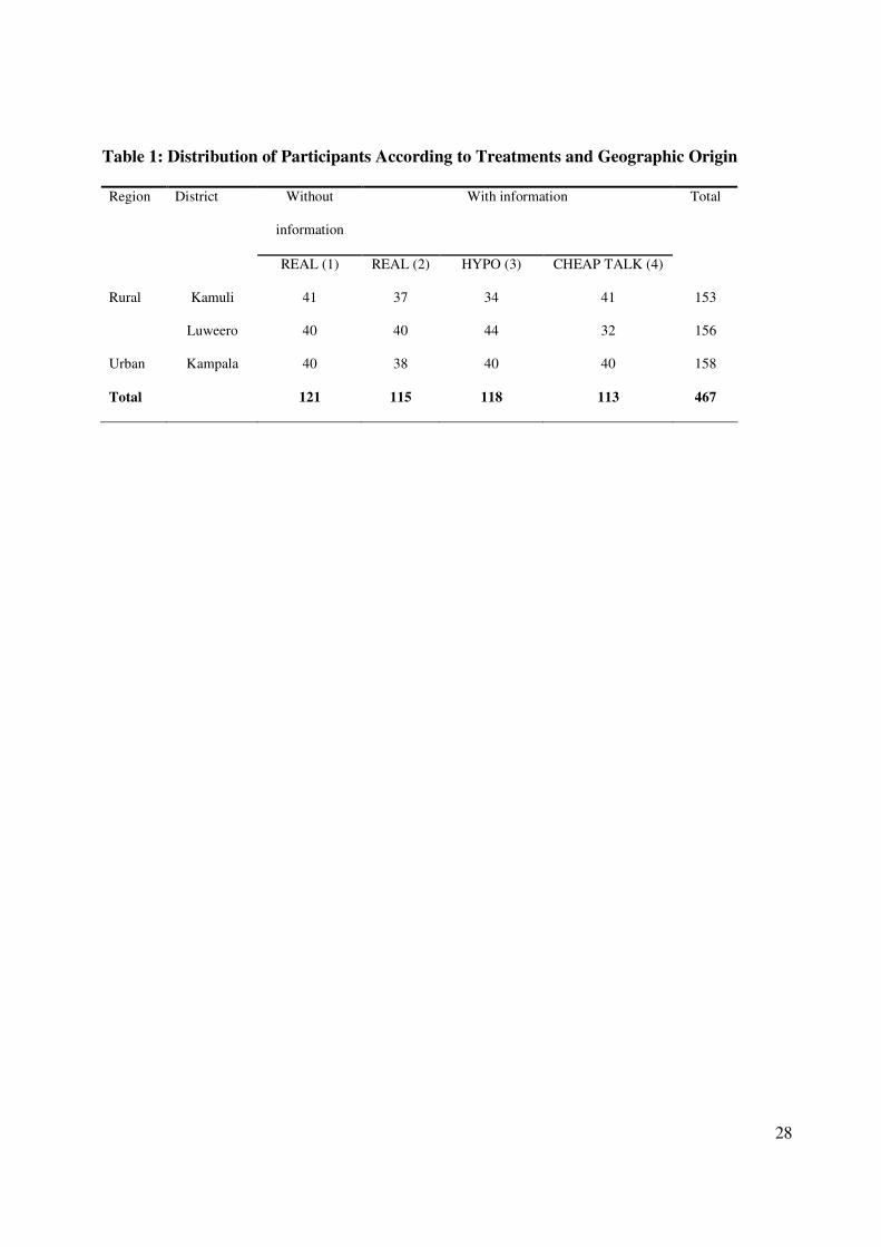
An almost equal number of participants were drawn from the rural areas of two districts (Kamuli and

Luweero) and one urban district (Kampala). Table 1 shows the distribution of participants across

treatments and their geographic origin.

[Insert Table 1 here]

8

In rural areas, participants were drawn from two districts where OFSP is new to the population. Four

villages were selected from each district based on ethnicity and distance from the district headquarters.

Once selected, a systematic random sample of 40 households was drawn from each village, and the

heads or the spouse of the head of the selected households were invited to take part in the experiment.

For Kampla, the urban district, two market places were selected where low- and middle-income urban

consumers buy their sweetpotatoes for consumption. Consumers were selected randomly in cooperation

with the market management committee. Among the participants, around 69% were head of the

households and 31% were spouses of the head of the household. About 61% of the household heads

make the sweetpotato buying decision while about 23% of the spouses take the buying decision. The

rest of the time, the decision is taken by their children.

The Varieties

For each treatment, consumers were exposed to the traditional white variety and two OFSP varieties,

one of which was deeper orange in color than the other. These were grown out for use in the study by

the National Agricultural Research Organization of Uganda. Those who received nutrition information

were told that there was a positive association between the color of the sweetpotato and its beta-

carotene content. A fourth variety that is yellow in color was also included, although the yellow

varieties are not nutritionally enhanced. Thus, there were four varieties of sweetpotato cultivars in all:

i) WHITE (Nakakande variety); ii) YELLOW (Tanzania variety); iii) ORANGE (SPK004/1/1 variety);

and iv) DEEP ORANGE (Ejumula variety). Each participant valued all four varieties, and the varieties

remained constant across treatments. As noted earlier, each individual participated in only one

treatment where the selection to a treatment was randomly assigned.

Experimental Procedure

The experiment followed the following sequence of steps: step-1: sensory acceptability; step-2:

provision of nutritional information to appropriate treatment arms; step-3: choice experiment (CE);

step-4: demographic module. Participants were organized in groups of four and were randomly

assigned among four treatments. Each participant was given UGS500 (about the equivalent of 30 US

9

cents) at the beginning of the experiment for participation, which s/he could keep or spend during the

experiment depending on the treatments assigned and choices made. Participants who were assigned in

hypothetical and real treatments went through all four steps. Participants who were assigned in real

without information went through step-1, step-3, and step-4.

Sensory acceptability

Each participant tasted a portion (30g to 50g) of each cooked sweetpotato variety (simultaneously

presented in random order and coded with three figure random numbers on white paper plates). The

samples were prepared in a way similar to that normally used by Ugandan households for their own

consumption. Fresh sweetpotato roots were sorted to remove diseased and insect damaged ones, peeled

and cut into roughly equal sized portions (5 to 10 cm) and boiled until the texture, assessed by a fork,

was considered correct for eating. During testing fresh samples of cooked sweetpotato were frequently

prepared. The four varieties were scored for a) taste; b) appearance; and c) overall acceptability, using a

nine point hedonic scale. The administrator explained the score sheet to participants on a one-to-one

basis. The process followed here is similar to that is usually followed in food science for collecting

information on consumer acceptance of products (Tomlins et al., 2005, Tomlins et al., 2007). The score

sheet used in the experiment is given in Appendix 1.

Nutritional Information

Participants selected for the three treatments with information (treatments 2, 3 and 4) were given

nutritional information on OFSP by one administrator. The nutritional message that was given to

participants is similar to the one that implementing NGOs were planning to us in OFSP promotion in

Uganda. The message is attached in Appendix 2.7 Respondents who took part in the real treatment

without information (treatment 1) did not receive any information. These subjects were asked about

whether they had any prior information on OFSP; this information is used as a control variable in the

empirical estimation.

7 We are grateful to Anna-Marie Ball for providing us with this information.

10

Choice Experiment

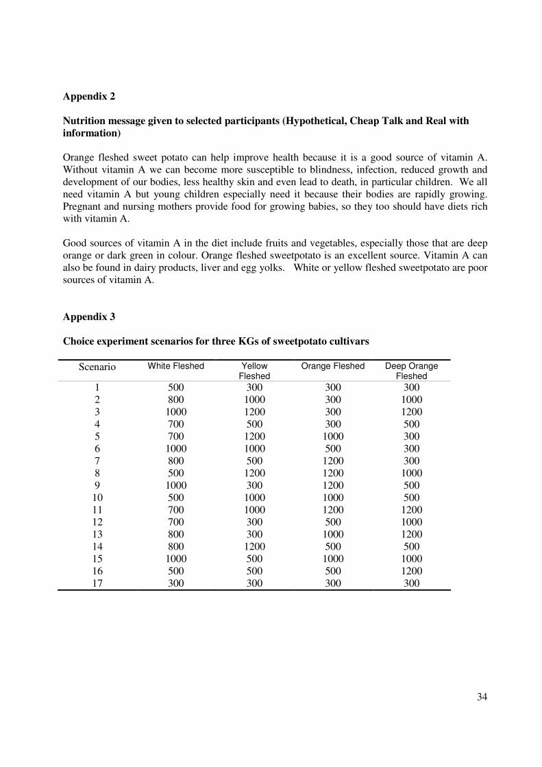
All participants then proceeded to the choice experiment and were given a choice sheet that contained

seventeen repeated CE questions (see the Appendix 3 for CE scenarios). The administrators worked on

a one-on-one basis, and explained instructions to the subjects. In the instructions, we followed

Cummings and Taylor (1999), List (2001), and List et al (2006), with necessary changes due to

differences in goods and allocation mechanism (see the Appendix 4 for subject instructions).

Participants responded to a series of 17 CE questions. Subjects taking part in hypothetical treatments

were instructed that “… choices that you will make are hypothetical and no purchase will take place.”

Subjects assigned to the two real treatments were informed that after completing all CE questions, one

number out of 17 would be randomly selected as binding for which actual payment would occur.

Prices of traditional varieties of sweet potatoes were collected from the local market places

immediately prior to the experiment. Sweet potatoes in Uganda are usually sold in heaps (supermarkets

in Kampala are the exceptions that sell in KGs) where each heap varies from three to five KGs

depending on the seasons. In our experiment, we kept the weight of heaps constant at three KGs for all

varieties across treatments. The prices of the WHITE variety were varied between UGS500, UGS700,

UGS800, and UGS1000. These encompassed the minimum and the maximum prices of traditional

sweet potatoes observed in Uganda (again, with the exception of supermarkets in Kampala). For the

OFSP for which market price did not exist, we had focus group discussions and local experts’ opinions;

and prices were varied between UGS300, UGS500, UGS1000, and UGS1200. These were constructed

as ±one standard deviation from the minimum and maximum price of the traditional variety.8 A ‘none

of these’ option, in addition to four products, was also included that acts as a base from which other

alternatives are compared (Louviere, 1988).

Ideally, a consumer’s valuation of a product depends on various attributes such as taste, appearance,

nutritional value etc. However, consideration of all the dimensions simultaneously makes a choice set

too large to be manageable. The choice set given to the respondents was prepared by using a fractional 8 The standard deviation is 208.177. However, in Uganda, the minimum denomination of exchange usually used is UGS50. As a result, the prices were kept in-line with the common denomination of exchange.

11

factorial design. It is similar to the one used in Lusk and Schroeder (2004), which represents a suitable

fraction of all possible combinations of factor levels, and captures the main effects for each factor level.

It, in addition, also avoids multicollinearity and ensures that prices of each product are totally

uncorrelated with the prices of each of the other three products.

Demographic Module

The experiment was followed by a survey that collected information on income, demography,

nutritional information and awareness, consumption, production, buying and selling behavior. These

variables were then used to provide additional controls in the estimation of their willingness to pay.

The Econometric Model

To estimate consumers’ valuation for different varieties of sweetpotato, a universal logit model that

estimates the impact of prices on four different varieties – WHITE, YELLOW, ORANGE, and DEEP

ORANGE sweet potatoes has been estimated. The reference alternative consists of “none of these”- that

means, not choosing any of the four varieties.

In the universal logit model, the ith subject’s utility, if s/he chooses j variety of sweetpotato, is given by

(3) ijiik

ikjkjij XcPabV ε+′++= �=

5

1

Here j=1…5, k=1…5, bj is variety specific constant, ajk is the effect of kth variety’s price on the utility

of the jth variety, Pik is the kth variety price for the subject i, Xi is a vector of observed subject specific

characteristics including variables such as subject’s age, schooling, income and other household

characteristics. Note that unlike multinomial logit, both the subject specific characteristics and choice

specific characteristics are allowed here to affect the utility of all choices. A subject chooses Vij if

Vij>Vik for all other k possible choices. It is assumed that ijε is independent and follows a type 1

extreme value distribution given by exp[-exp(- ijε )] which assumes that the omission of an irrelevant

choice set should not change the parameter estimates.

12

Unlike multinomial logit (MNL), the universal logit model specified above relaxes the MNL cross

elasticity properties by including attributes of competing alternatives in the utility function for all

alternatives in the choice set (McFadden, Train and Tye, 1978). To test the independence of irrelevant

alternatives (IIA) assumption, the appearance of significant cross-effects for the effect of alternative k

would imply that the utility of an alternative depends on the attributes of other alternative(s), and

therefore IIA assumption no longer holds. Though not the central focus, an examination of the results

shows that cross-effects of some of the attributes of interest, such as price and taste, are different from

zero, and therefore, the selection of universal logit over MNL is justified9.

Since the IIA property is violated, we have estimated a multinomial probit (MNP) model that does not

assume errors are independently distributed across alternatives. The probability that subject i chooses

alternative j is given by:

(4) 1... ... ( ) ...j j k j j JV V V V

ij jP f d dε ε

ε ε ε+ − ∞ + −

−∞ −∞ −∞= � � �

where J are the alternatives and ( )f ⋅ is a J-variate normal density function with mean zero and

J J× covariance matrix Σ (Louviere et al 2000, Lusk and Schroeder 2004). As we will see in the

next section, the estimated WTP and marginal WTP based on MNP model are not statistically different

from those obtained from the universal logit model.

As described in the Experimental Design Section, we have repeated observations, seventeen to be

precise, per subject. It is likely that errors are correlated over repeated observations for a given subject

and within-subject clustering is needed. In the universal logit estimation, we therefore treated each

9 Models that relax the IIA assumption are discussed in Results Section.

13

subject as a cluster.10 In addition, we have estimated fixed-effects logit model for panel data

(Chamberlain 1980) in which the probability that alternative j is chosen by subject i is give by:

(5)

1

exp( )

exp( )

ijij J

i ijj

VP

V

µ

µ=

=�

where � is a positive scale parameter.

In estimating WTP and marginal WTP, we are also concerned with the probable heteroskedasticity

since error variance may not be constant across subjects or alternatives. To account for possible

heteroskedasticity correction, we have estimated a heteroscedastic conditional logit model11 in which

the probability that alternative j is chosen by subject i is give by (Hole 2006):

(6)

1

exp( )

exp( )

i ijij J

i ijj

VP

V

µ

µ=

=�

Where �i is scale parameter. It is a function of individual characteristics that influence the magnitude of

the scale parameter and therefore the error variance. Here �i is parametrised as exp(Xi�) where Xi is a

vector of observed subject specific characteristics as described above. A test for �=0 is a test for the

error variance being constant across subjects. As we will see in the result section, Lagrange multiplier

test for heteroscedasticity reveals that the presence of heteroscedasticity cannot be rejected.

Finally we estimate a mixed logit model12 which is free of any restrictive assumptions such as IIA and

allows taste parameters to vary in the population. We modify equation (1) to express the utility that

subject i gets from choosing alternative j is given by:

10 However, controlling for clustering increases standard errors, especially for regressors that are highly correlated with the cluster (Cameron and Trivedi 2009, pp.306-307). 11 This model is also referred to as the parametrised heteroscedastic multinomial logit model (Hensher et at., 1999). 12 This model is also referred to as the random parameter logit model (Lusk and Schroeder 2004).

14

(1’) 'ij ij i ijU β ε= +x

(7) i i iβ β η= + +z

where xij is the full vector of observed characteristics including the attributes of alternatives described

above, ijε are iid extreme value, zi is observed data and iη is an additional error term. The

unconditional probability that subject i chooses alternative j is given by (Hensher et al 2005):

(8) ( , ) ( , )i

ij ij i i i i i iP L f dβ

β η η η= � x z �

In estimating the mixed logit model, the alternative-specific constants are assumed to be independently

normally distributed in the population while other coefficients including price are assumed fixed. The

model has been estimated by using maximum simulated likelihood (Train 2003, Hole 2006).

Demographic variables such as family size, number of children under the age of five years, and the

presence of pregnant women and breastfeeding mothers can have significant influence on household

consumption decision (Pollak and Wales 1981). Such variables have been included in the WTP analysis

to see the conditional preferences for OFSP.

[Insert Table 2 here]

Table 2 provides summary statistics on the demographic characteristics of the respondents in the four

different treatment arms, as well as information on their incomes and any prior information on OFSP. It

is clear that there is no significant difference among four different treatments in respect of individual

characteristics. This ensures that there was no systematic bias in subject selection among treatments,

and that the random assignment of subjects on four different treatments was properly done.

15

Results

Table 3 reports parameter estimates of full sample and all four treatments estimated by the universal

logit model. Only the variety specific constants (bj of equation 3) and own-price effects (aj of equation

3) are reported in Table 3.

[Insert Table 3 here]

We have repeated observations, seventeen to be precise, per subject, which we treated as a cluster. It is

likely that errors are correlated over repeated observations for a given individual and within-individual

clustering is needed. However, controlling for clustering increases standard errors, especially for

regressors that are highly correlated with the cluster (Cameron and Trivedi 2009, pp.306-307).

The test for parameter equality across treatments, (given by )(2 �−− ij LLLL , which is distributed

as 2χ with K(M-1) degrees of freedom, where LLj is the log likelihood value for the full sample, and

LLi is the log likelihood value for each of the treatments, K is the number of restrictions, 17, and M is

the number of treatments, 4 (Lusk and Schroeder 2004, Louviere, Hensher and Swait 2000) is strongly

rejected ( 2χ =1959.9; p<0.01). Hence, in the rest of the paper, we report results based on the four

separate treatments, and not those for the pooled full sample.

Second, to test the validity of IIA assumption, we implement Hausman’s specification test, which

suggests that the omission of an irrelevant choice set should not change the parameter estimates

(Hausman and McFadden, 1984). The test rejects the assumption of IIA.13

How much consumers value a particular variety of sweetpotato j is obtained as the ratio of variety

specific constant to the price coefficient ( jj ab /− ). Table 4 reports the willingness-to-pay (WTP) for

13 For the full sample, the chi2 (37)=(b-B)'[(V_b-V_B)^(-1)](b-B)=65.47, prob>chi2=0.0027. The test statistics for others are available upon request.

16

each variety calculated from the parameters (reported in Table 3) estimated by the universal logit model

(Equation 3). The reported WTPs are for one KG of sweetpotato (Table 4). Standard errors of WTP are

generated through parametric boot strapping method and reported in Table A1 in Appendix 5.

The marginal willingness-to-pay for a particular OFSP j versus traditional white variety k is calculated

as the difference in willingness-to-pay between j and k ( kkjj abab // +− ). Table 4 also reports these

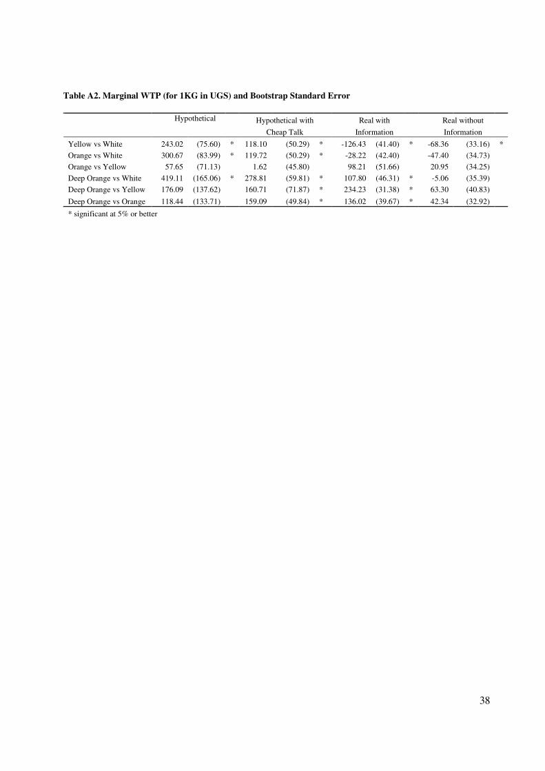
marginal WTP estimates, while the corresponding boot-strapped standard errors are in Table A2.

[Insert Table 4 here]

Willingness to pay (WTP) for OFSP in the absence of nutrition information

The WTP estimates obtained in the treatment “real without information” suggest that relative to the

familiar white varieties, there is no difference in the willingness to pay for deep orange sweet potato.

This is however not true for the other orange variety, for which consumers appear to be willing to pay

less than they would for the white variety; suggesting that it’s sensory characteristics may adversely

affect consumers’ valuation. In addition, the yellow variety commands a statistically significant and

substantial discount of nearly 30%.. These results suggest that in the absence of an information

campaign, new varieties including OFSPs, if accepted by farmers, may suffer a price disadvantage in

the market, and there is clearly no premium for the orange taste either.

The impact of nutrition information

The provision of nutrition information translates into a premium for the orange varieties between

treatments. The difference in WTP between the two real treatments—with and without information—

indicates an increase of UGS 32 per kg and UGS 126 per kg, respectively, both of which are

statistically significant. With knowledge of the nutritional value, there is a substantial premium for the

deep orange varieties relative to white, which is also significant, unlike the case when no information

was provided. The WTP for deep orange varieties is nearly 40% higher than that for the white.

17

These premia are in line with the findings of McGuirk et al. (1995) and Kinnucan et al. (1997), who

find a significant impact of health information on food demand in the United States.14 The magnitude of

the premium for deep orange varieties when nutrition information is provided is line with those found

in other studies: a 25-50% premium for non-GMO foods are reported in Europe and Japan, although the

magnitudes are far more modest in the United States (see for example Li, McCluskey and Wahl, 2004).

Nevertheless, given the developing country setting of the study, the premia for nutrition information

appear high, given the relatively limited purchasing power of most study participants, and the salience

of a staple food in average budgets in countries such as Uganda. One explanation may be that the

nutritional information was given in a one-to-one setting; making it the most effective and perhaps the

most costly form of communication. This might have biased upward the size of the impact due to

nutritional information and may well have been lower had other forms of communication been used.

Has one-to-one interaction between subjects and experimenter resulted in upward bias? Our assumption

was that the subjects’ expected experiment objectives are orthogonal to the true objectives and

predictions, and they do not plausibly imply actions on behalf of subjects. However, looking at the

results, the experimenter demand effects cannot be entirely ruled out. However, we needed to weigh

between the experimental objectives and possible limitations. Eliciting valuation in rural communities

in developing countries through choice experiment or similar mechanisms requires one-to-one

interaction between experimenter and subjects. The low level of formal schooling (less than seven years

in our sample, see Table 2) makes it extremely difficult to minimize experimenter’s presence. This does

not necessary mean that the experimental results are confounded. The nutritional information campaign

designed by NGOs to promote OFSP involves face-to-face communication. Therefore, the experimental

setting mimics the actual strategy that will be followed in the future.

����������� ����� � ������ ����������������� �������������������� ��� �������������������� �����������������

������ ������������� ��

18

However, the impact of prior information is negative and significant (see Table 5), which is puzzling.

Since our data does not have any further details on the sources and nature of prior information received

by subjects, the issue remains underexplored. However, a simple comparison of the mean WTP

between two groups, those who received prior information and those who did not in treatment 3 shows

that the latter group is willing to pay more than 7% higher for the deep orange variety of OFSP.

The magnitude of hypothetical bias

The extent to which WTP for new products, and the marginal WTP for nutrition information, can be

accurately assessed in a hypothetical setting can be seen by comparing the magnitudes of WTP in

treatments (2) and (3) in Table 4. It is evident that in the absence of a cheap-talk script, hypothetical

bias is large: on average, participants overstated their WTP by a factor of above 2 in hypothetical

scenarios compared to real scenarios. This supports the findings reported in List and Gallet (2001). In

addition, the marginal WTP estimates from the hypothetical choices are also overstated. As might be

expected, the degree of hypothetical bias for white varieties is minimal, since this is the product with

which consumers are familiar. Note that unlike the case in most hypothetical elicitation experiments,

consumers in Uganda had an opportunity to taste the three products that they were being asked to

assess. So the difference in the ‘real’ and ‘hypothetical’ arms cannot be attributed to their exposure to

the product, but entirely to the fact that in the real treatment, respondents had to make a purchase, but in

the hypothetical arm, they did not have to do so.

The mitigation of hypothetical bias through cheap talk

Turning to the effectiveness of cheap talk in mitigating hypothetical bias, the results suggest that

although the use of a cheap talk script does result in a reduction in the magnitude of the willingness to

pay, the bias remains substantial. This finding is of interest because unlike most other cheap talk

scripts, such as those used by Cummings and Taylor (1999) and List (2001) which explicitly indicate

the direction of bias, the cheap talk script used in this study was deliberately neutral in its wording.

Nonetheless the cheap talk had the desired effect of lowering hypothetical bias, although it did not

eliminate it. For example, while the WTP for deep orange in the hypothetical arm was 750 UGS/kilo,

19

more than double the UGS 357 in the real arm, with cheap talk the WTP estimates drop to UGS

553/kilo, considerably lower than 750, but still much higher than the 357. Upward biases are also seen

in the estimated marginal willingness to pay for orange and deep orange varieties as well, although

once again these biases are lower than was the case in the hypothetical scenario without using a cheap

talk script.

The correlates of willingness to pay

To examine how the taste, income and demographic factors influence WTP, Table 5 presents the

estimated coefficients of the universal logit model for the real treatment with information.15

[Insert Table 5 here]

Though the income coefficient is positive, it is not significant. Since sweetpotato is one of the prime

staple foods for the participants in this study, this is not an unexpected result.16 Taste factors are also

important: all own-taste and most cross-tastes coefficients are significant (Table 5). These also

provide a justification for the inclusion of a consumer acceptance taste test prior to the CE, although

collinearity problems precluded the inclusion of all the sensory variables17. Urban/rural differences in

WTP and marginal WTP are captured in two rural district dummies. Rural households have a lower

WTP for the traditional variety of sweetpotato but have a higher WTP for varieties with higher �-

carotene content sweetpotatoes (based on real treatment with information).

Results obtained from alternative models

Parameter estimates (variety specific constant and own-price effects) and the associated WTP and

MWTP obtained from alternative models that do not put IIA restrictions (multinomial probit model,

15 We present the parameter estimates only of one of the treatments; the coefficients in the other treatments have by and large the same sign. The full set of estimates is available from the authors on request. 16 To see if alternative measure of income such as land ownership has any impact, we replaced income with land. The results are reported in Table A3 in Appendix. For two orange varieties, land-ownership has positive and significant effect. 17 The pair-wise correlation coefficient between taste and overall acceptability for each of the four samples is a high 0.9.

20

and mixed logit model), that takes the repeated nature of the data into account (fixed-effects logit

model), that corrects for possible heteroscedasticity (heteroscedastic conditional logit model), and that

allows taste parameters to vary across varieties are presented in Table A4 in Appendix. The results

show that WTP and marginal WTP obtained from alternative models are not statistically different from

those obtained from the universal logit model. However, the maximum likelihood test conducted after

the estimation of heterscedastic conditional logit model rejects the assumption that error variances are

constant across subjects. Turning to the mixed logit results, except for the deep-orange, the variety-

specific random parameter estimates are not statistically significant. However, for the deep-orange

variety, the random parameter estimate suggests the existence of heterogeneity over the sampled

population.

Preference consistency

In its simplest form, a WARP violation occurs if a subject chooses a particular variety of sweetpotato

(e.g., WHITE) in one scenario when another variety of sweetpotato (e.g., ORANGE) is less expensive,

but chooses ORANGE in a different scenario when WHITE was less expensive. We had 17 choice

scenarios; each subject went through all the 17 choice scenarios and made her/his choice in each of the

scenarios. Around 30% of the subjects violated the WARP at least in one circumstance. This is similar

to what reported in List et al (2006).

To see if WARP violation tends to increase with the increasing number of scenarios, we looked at the

correlation between choice scenarios and WARP violation, which is 0.18. This indicates the presence of

survey fatigue from the survey administrators or subjects’ part. To see if violation has any systematic

link with the administrators’ characteristics, we looked at the number of violations occurred with each

of the six administrators. We had six administrators who were locally recruited and trained by us.

However, we have not found any systematic relationship between administrators’ observed

characteristics such as gender (we had three male and three female experimenters), age or education (all

of them were recent graduates from local universities in economics or computer sciences). To explore

further, we estimated a probit model of WARP violation on subjects observed characteristics that

21

included gender, education and income and other demographic characteristics. Again, we did not find

any systematic relationship between subjects’ observed characteristics and WARP violations.

In terms of the violations by treatments, the highest number WARP violation occurred in the

hypothetical treatment with cheap talk (29.24%) and the lowest number of WARP violation occurred in

real treatments (13.08%). List et al (2006) reports a similar result from a choice experiment that they

conducted in the USA. In their experiment, the proportions of subject with inconsistent preference were

24.5% and violations increased in hypothetical treatment with cheap talk (33.9%), which is slightly

higher than the number of violations occurred in the current experiment. Again, this might add further

question to the validity of cheap talk, which may reduce hypothetical bias but introduces a new bias

into subject’s decision making.

This may suggest that using as many as 17 choice sets and “cheap talk” may be problematic; this is an

area for further research.

Conclusions

We used real money and real products to compare the willingness to pay for sweetpotatoes that are both

traditional (white and yellow) and that are biofortified (orange and deep orange), and compared these

with results constructed from hypothetical scenarios. We also relied on methods from food science to

enable consumers to taste the products that they would be asked to value.

Our results confirm the presence of hypothetical bias reported in literature. It is therefore important to

introduce and work with the real product in order to elicit accurate estimates of the WTP and marginal

WTP for biofortified crops in developing country settings.

The introduction of a cheap talk script does result in a significant reduction in valuations, even when

the script does not mention the direction of possible bias. However, the estimated WTP and marginal

22

WTP are higher than those obtained in the real treatment, suggesting that while the bias is reduced it is

not eliminated. The additional expense of working with real incentives and products appears justified.

Turning to the scenarios using the real product, our results for Uganda, a key target country for the

orange-fleshed sweetpotato suggest that in the absence of a promotional campaign, OFSP varieties, on

an average, are likely to compete on par with the traditional white varieties in the market. To the extent

that sweetpotato is produced and consumed on-farm, provided the agronomic properties are acceptable

to farmers, there may not be any significant discount in the market. Our post-experimental inquiry

reveals that OFSP that are currently sold in the market are sold at a price similar to the traditional white

varieties. However, the supply of OFSPs remains very limited at this stage and they are often not sold

separately- rather mixed with traditional varieties.

The impact of nutrition information is substantial. When informed about the nutritional value of the

OFSP, consumers are willing-to-pay a premium, and the size of the premium is higher for the deep

orange than for the orange; the deep orange has more beta-carotene than the orange. However, given

the one-to-one communication, the possibility of the experimenter demand effect on the subjects cannot

be entirely ruled out.

This paper represents perhaps one of the few examples where choice experiments have been conducted

in a developing country setting, using rural and urban consumers. Our results provide a validation of

the use of choice experiments in developing country settings, although the percentage of respondents

who exhibited inconsistent switches in preferences is somewhat high, especially in hypothetical

treatment with cheap talk.

23

References

Black, R.E., L.H. Allen, Z.A. Bhutta, L.E. Caulfield, M.de Onis, M. Ezzati, C. Mathers, and J. Rivera.

2008. “Maternal and Child Undernutrition: global and regional exposures and health

consequences.” Lancet 371 (9608): 243-260.

Bouis, H.E. 1999. “Economics of Enhanced Nutrition Density in Food Staples.” Field Crops Research

60 (1-2): 165-173.

Cameron, C., and P. Trivedi. 2009. Microeconometrics Using Stata. Texas: Stata Press.

Carlsson, F., P. Frykblom and C.J. Lagerkvist. 2005. “Using Cheap Talk as a Test of Validity in

Choice Experiments.” Economics Letters 89:147-152.

Chalfant, J.A., and J.M. Alston. 1988. “Accounting for Tastes.” Journal of Political Economy 96(2):

391-410.

Chamberlain, G. 1980. Analysis of covariance with qualitative data. Review of Economic Studies 47:

225-238.

Cummings, R. and L. Taylor. 1999. “Unbiased Value Estimates for Environmental Goods: A Cheap

Talk Design for the Contingent Valuation Method.” American Economic Review.89(3): 649-65.

Frykblom, P. 1997. “Hypothetical Question Modes and Real Willingness to Pay.” Journal of

Environmental Economics and Management 34 (1): 275-287.

Hasuman, J. and D. McFadden. 1984. “Specification Tests for the Mulitnomial Logit Model.”

Econometrica 52(4): 1219-40.

Hensher, D., J. Louviere, J. Swait. 1999. Combining Sources of Preference Data. Journal of

Econometrics 89, 197-221.

Hensher, D., J. Rose, W. Greene. 2005. Applied Choice Analysis A Primer. Cambridge: Cambridge

University Press

Hole, A.R. 2006. Small-sample properties of tests for heteroscedasticity in the conditional logit model.

Economics Bulletin 3: 1-14.

Hole, A.R. 2007. Fitting mixed logit models by using maximum simulated likelihood, Stata Journal,

StataCorp LP, 7(3):388-401.

24

Kinnucan, H.W., H. Xiao, C.J. Hsia, and J.D. Jackson. 1997. “Effects of Health Information and

Generic Advertising on US Meat Demand.” American Journal of Agricultural Economics 79(1):

13-23.

Lancaster, K. 1974. “A New Approach to Consumer Theory.” Journal of Political Economy, 74(1):

132-157.

Li, Q., J.J. McCluskey, and T.I. Wahl. 2004. “Effect of Information on Consumers’ Willingness to Pay

for GM-Corn-Fed Beef.” Journal of Agricultural and Food Industrial Organization 2: Article 2.

List, J.A. 2001. “Do Explicit Warnings Eliminate the Hypothetical Bias in Elicitation Procedures?

Evidence from Field Auctions for Sportscards.” American Economic Review 91(5): 1498-1507.

List, JA., and C. Gallet. 2001. “What Experimental Protocol Influence Disparities Between Actual and

Hypothetical Stated Values? Evidence from a Meta-Analysis,” Environmental and Resource

Economics 20(3): 241-254

List, JA., P. Sinha, and M.Taylor. 2006. “Using Choice Experiments to Value Non-Market Goods and

Services: Evidence from Field Experiments.” Advances in Economic Analysis and Policy 6(2),

Article 2.

Louviere, J.J. 1988. “Conjoint Analysis Modeling of Stated Preferences: A Review of Theory,

Methods, and Recent Developments and External Validity.” Journal of Transport Economics and

Policy 10: 93-119.

Louviere, J.J., D.A. Hensher, and J.D. Swait. 2000. Stated Choice Methods: Analysis and Application:

Cambridge University Press.

Low, J.W., M. Arimond, N. Osman, B. Cunguara, F. Zano and D. Tschirley. 2007. “A Food-Based

Approach Introducing Orange-Fleshed Sweet Potatoes Increased Vitamin A Intake and Serum

Retinol Concentrations in Young Children in Rural Mozambique”. Journal of Nutrition

137:1320-1327.

Lusk, J.L., and T.C. Schroeder. 2004. “Are Choice Experiments Incentive Compatible? A Test with

Quality Differentiated Beef Steaks.” American Journal of Agricultural Economics 86(2): 467-

482.

25

McFadden, D., K. Train, and W.B. Tye. 1978. “An Application of Diagnostic Tests for the

Independence From Irrelevance Alternatives Property of the Multinomial Logit Model.”

Transportation Research Record: Journal of the Transportation Research Board 637: 39-46.

McFadden, D. 1974. “Conditional Logit Analysis of Qualitative Choice Behavior,” in Frontiers in

Econometrics, P. Zarembka, ed., New York: Academic Press.

McGuirk, A., P. Driscoll, J. Alwang, and H. Huang. 1995. “System Misspecification Testing and

Structural Change in Demand for Meats.” Journal of Agricultural and Resource Economics 20: 1-

21.

Pollak R.A., and T.J. Wales. 1981. “Demographic Variables in Demand Analysis.” Econometrica 49:

1533-51.

Robenstein, R.G. and W.N. Thruman 1996. “Health Risk and the Demand for Red Meat: Evidence

from Futures Markets.” Review of Agricultural Economics 18: 629-41.

Sommer, A., K.P. West, J.A. Olson, A.C. Ross. 1996. Vitamin A Deficiency: Health, Survival, and

Vision. New York, Oxford University Press.

Stigler, G. and G. Becker. 1997. “De Gustibus Non Est Disputandum.” American Economic Review 67:

76–90.

Tomlins, K. I., J.T. Manful, P. Larwer. and L. Hammond. 2005. “Urban consumer acceptability and

sensory evaluation of locally produced and imported parboiled and raw rice in West Africa.”

Food Quality and Preference 16, 79-89.

Tomlins, K.I., J. Manful, J. Gayin, B. Kudjawu and I. Tamakloe. 2007. “Study of sensory evaluation,

consumer acceptability, affordability and market price of rice.” Journal of the Science of Food

and Agriculture, 87, 1564 - 1575.

Train, K. E. 2003. Discrete Choice Methods with Simulation. Cambridge: Cambridge University Press.

van Jaarsveld, P.J., F. Mieke, S.A. Tanumihardjo, P. Nestel , C.J. Lombard, and A.J.S. Benade, 2005.

“�-carotene-rich Orange-fleshed Sweetpotato Improves the Vitamin A Status of Primary School

Children Assessed with Modified-relative-dose-response Test.” American Journal of Clinical

Nutrition 81:1080-1087.

26

West Jr., K. and I. Darnton-Hill. 2001. “Vitamin A Deficiency. Nutrition and Health in Developing

Countries” In: Richard D. Semba and Martin W. Bloem (eds.), Nutrition and Health in

Developing Countries, NJ: Humana Press, 267-306.

27

Tables and Figures

Figure 1: The Field Design

Without Nutrition

Information

With Nutrition

Information

Real (1) (2)

Hypothetical, no cheap talk (3)

Hypothetical, with cheap talk (4)

28

Table 1: Distribution of Participants According to Treatments and Geographic Origin

Region District Without

information

With information Total

REAL (1) REAL (2) HYPO (3) CHEAP TALK (4)

Kamuli 41 37 34 41 153 Rural

Luweero 40 40 44 32 156

Urban Kampala 40 38 40 40 158

Total 121 115 118 113 467

29

Table 2: Variable Definitions and Summary Statistics

Variable Definition Full Sample Real, without information

Real Hypothetical Cheap Talk

With information Taste Participants' relative preference

among the four varieties

White % of participants who preferred the white variety most 9.24 12.61 10.68 7.96 5.66

Yellow % of participants who preferred the yellow variety most 26.10 22.52 22.33 23.89 35.85

Orange % of participants who preferred the orange variety most 13.16 14.41 11.65 13.27 13.21

Deep orange % of participants who preferred the deep orange variety most 51.50 50.45 55.34 54.87 45.28

Demography and Income

Gender % of male 0.455 0.423 0.505 0.460 0.434

(0.006) (0.011) (0.012) (0.011) (0.012)

Education Years of schooling 6.393 5.973 6.735 6.463 6.444

(0.041) (0.074) (0.090) (0.161) (0.082)

Family Size Number of members in the household 6.136 5.865 6.282 6.354 6.047

(0.056) (0.089) (0.087) (0.011) (0.077)

Children under 5 Number of children under the age of five 1.388 1.351 1.485 1.274 1.453

(0.015) (0.035) (0.029) (2844.921) (0.027) Pregnant/Brest feeding

Number of pregnant/ breast-feeding women in the household 0.402 0.441 0.359 0.310 0.500

(0.007) (0.015) (0.012) (0.011) (0.014)

Income Household income in UGS/year 83282 81685 94073 80333 93320

(81281) (135195) (87667) (83453) (77942) Prior Information on OFSP

% of participants who received information on OFSP 0.383 0.288 0.272 0.416 0.557

prior to the experiment (0.006) (0.010) (0.011) (0.011) (0.012)

Kampala # of observations from Kampala 2686 680 646 680 680

Kamuli # of observations from Kamuli 1,955 527 425 493 510

Luweero # of observations from Luweero 2,720 680 680 748 612 Standard errors are in parentheses.

30

Table 3: Parameter Estimates – Universal Logit Model Variety specific constant Full sample

Real without Information (1)

Real with Information (2)

Hypothetical, no cheap talk (3)

Hypothetical, with Cheap Talk (4)

White 9.344 (0.616) 16.786 (1.625) 5.660 (1.411) 5.825 (1.801) 15.904 (1.965)

Yellow 6.854 (0.516) 5.500 (1.064) 3.435 (1.207) 9.994 (1.628) 11.548 (1.370)

Orange 7.196 (0.493) 5.001 (1.061) 5.547 (0.987) 10.283 (1.582) 11.662 (1.339)

Deep orange 7.298 (0.466) 6.421 (1.114) 7.110 (0.856) 9.021 (1.550) 11.901 (1.234)

Own-price effects

White -0.010 (0.001) -0.024 (0.002) -0.008 (0.001) -0.006 (0.001) -0.019 (0.002)

Yellow -0.007 (0.000) -0.011 (0.001) -0.009 (0.001) -0.006 (0.001) -0.010 (0.001)

Orange -0.006 (0.000) -0.009 (0.001) -0.008 (0.001) -0.005 (0.001) -0.010 (0.001)

Deep orange -0.005 (0.000) -0.009 (0.001) -0.007 (0.000) -0.004 (0.000) -0.007 (0.001)

Log Likelihood -5124 -872 -985 -1368 -919

No. of observations 6640 1760 1568 1728 1584 Numbers in the parentheses are standard errors

31

Table 4: Willingness-To-Pay (WTP) and Marginal Willingness-To-Pay (WTP) for OFSP (UGS/Kg) Real without Real with Hypothetical Hypothetical with

Information

(1) Information

(2)

(3) Cheap Talk

(4) Total WTP

White 237 250 331 274 Yellow 168 123 574 392 Orange 189 221 631 394 Deep Orange 232 357 750 553

Marginal WTP Yellow vs White -68 (29%) -126 (50%) 243 (73%) 118 (43%) Orange vs White -47 (20%) -28 (11%) 301 (91%) 120 (44%) Orange vs Yellow 21 (11%) 98 (44%) 58 (9%) 2 (1%) Deep Orange vs White -5 (2%) 108 (43%) 419 (127%) 279 (102%) Deep Orange vs Yellow 63 (27%) 234 (66%) 176 (23%) 161 (29%) Deep Orange vs Orange 42 (18%) 136 (38%) 118 (16%) 159 (29%)

WTP values for 1 KG of sweetpotato

32

Table 5: Universal Logit Estimates – Real Treatment with Information White Yellow Orange Deep Orange

Coefficient Variety Variety Variety Variety

Price of white sweetpotato -0.00756*** -0.00142 0.000183 0.0000686

(0.0014) (0.0012) (0.0009) (0.0006)

Price of yellow sweetpotato 0.000198 -0.00929*** -0.00165*** -0.000227

(0.0007) (0.0009) (0.0005) (0.0003)

Price of orange sweetpotato -0.000187 0.00106 -0.00835*** -0.00133***

(0.0007) (0.0007) (0.0008) (0.0003)

Price of deep orange sweetpotato -0.000825 -0.000432 -0.000668 -0.00663***

(0.0007) (0.0006) (0.0005) (0.0004)

Gender 1.188*** -0.312 0.198 0.174

(0.4400) (0.2700) (0.2500) (0.2100)

Education 0.0879 0.126*** -0.0122 0.0666**

(0.0600) (0.0410) (0.0380) (0.0330)

Family size -0.0485 -0.0205 -0.133*** -0.0256

(0.0750) (0.0520) (0.0500) (0.0410)

Children under five 0.356 0.139 0.409*** 0.338***

(0.2700) (0.1500) (0.1300) (0.1100)

Pregnant/Breast feeding mother -0.127 -1.191*** -1.024*** -1.271***

(0.4500) (0.2800) (0.2500) (0.2100)

IncomeX10^5 0.0109 0.00954 0.0212 0.00723

(0.0190) (0.0180) (0.0180) (0.0160)

Prefer yellow variety -1.395** 2.681*** 2.867*** 1.075***

(0.5400) (0.4900) (0.4900) (0.4100)

Prefer orange variety -1.717** -0.326 2.091*** -0.635

(0.7100) (0.5400) (0.5100) (0.4400)

Prefer deep orange variety -4.690*** -0.373 1.001** 1.487***

(0.7300) (0.4300) (0.4100) (0.3500)

Prior information on OFSP -2.257*** -1.468*** -0.989*** -0.936***

(0.6900) (0.3500) (0.3100) (0.2700)

Kamuli district -1.827** 2.138*** 0.895** -0.0143

(0.8600) (0.4700) (0.4100) (0.3500)

Luweero district -0.249 1.675*** 0.773** -0.273

(0.5400) (0.4100) (0.3800) (0.3200)

Constant 5.660*** 3.435*** 5.547*** 7.110***

(1.4100) (1.2100) (0.9900) (0.8600)

Observations 1568

Log Likelihood -984.567

Standard errors in parentheses *** p<0.01, ** <0.05, * p<0.1

33

Appendix 1 Hedonic scale used by consumers for the acceptability (appearance, taste and overall) for cooked sweetpotato

Participant Number

Sample Code

Please taste the four samples on the plate in front of you. Each sample is identified by a code. Please tick each box according to how acceptable you find each sample for appearance, taste and overall acceptability

Appearance Taste Overall

acceptability

Like extremely

Like very much

Like moderately

Like slightly

Neither like nor dislike

Dislike slightly

Dislike moderately

Dislike very much

Dislike extremely

Comments

34

Appendix 2 Nutrition message given to selected participants (Hypothetical, Cheap Talk and Real with information) Orange fleshed sweet potato can help improve health because it is a good source of vitamin A. Without vitamin A we can become more susceptible to blindness, infection, reduced growth and development of our bodies, less healthy skin and even lead to death, in particular children. We all need vitamin A but young children especially need it because their bodies are rapidly growing. Pregnant and nursing mothers provide food for growing babies, so they too should have diets rich with vitamin A. Good sources of vitamin A in the diet include fruits and vegetables, especially those that are deep orange or dark green in colour. Orange fleshed sweetpotato is an excellent source. Vitamin A can also be found in dairy products, liver and egg yolks. White or yellow fleshed sweetpotato are poor sources of vitamin A. Appendix 3 Choice experiment scenarios for three KGs of sweetpotato cultivars

Scenario White Fleshed Yellow Fleshed

Orange Fleshed Deep Orange Fleshed

1 500 300 300 300 2 800 1000 300 1000 3 1000 1200 300 1200 4 700 500 300 500 5 700 1200 1000 300 6 1000 1000 500 300 7 800 500 1200 300 8 500 1200 1200 1000 9 1000 300 1200 500 10 500 1000 1000 500 11 700 1000 1200 1200 12 700 300 500 1000 13 800 300 1000 1200 14 800 1200 500 500 15 1000 500 1000 1000 16 500 500 500 1200 17 300 300 300 300

35

Appendix 4: Subject instructions Subject Instructions for the “Real” Treatment Now you have the opportunity to buy one of the four products that you just tested. They are arranged in 17 different scenarios. We would like you to make a choice in each scenario described below. In each scenario, there are four products that you just tested, and you may choose any of them. Alternatively, you may choose none of them. Once you have made your choice for each scenario, I will pick a number from the box that contains all scenario numbers (show them the box and the numbers inside). Each number has an equal chance to be picked. The number that I will pick will be the binding scenario. Only one of your choices will be binding. For example, if I pick 17, then the scenario number 17 will be binding. Depending on the choice that you have made, you will purchase the product or no purchase will be required if you have made “none of these” option in the binding scenario. Do you have any questions? Subject instructions for the “Hypothetical” Treatment Now imagine that you have the opportunity to buy one of the four products that you just tested. They are presented in 17 different scenarios. We would like you to make a choice in each scenario as if you were actually facing them in real life. In each scenario, there are four products that you just tested, and you may choose any of them. Alternatively, you may choose none of them. Note that all these choices that you will make are hypothetical and no purchase will take place. Cheap talk script (CT 1999, List 2001, List et al 2006) Before you make your choices, I want to talk to you about a problem that we have in studies like this one. As I told you a minute ago, this is a hypothetical choice – not a real one. No one will actually pay money at the end. But, I also asked you to choose as though the result would involve a real cash payment. And that’s the problem. In most studies of this kind, folks seem to have hard time doing this. They act differently in a hypothetical setting, where they don’t really have to pay money, than they do in a real purchase, where they really could have to pay money. For example, in a recent study, several different groups of people bid in an auction. Payment was hypothetical for these groups, as it will be for you. No one had to pay money if they won the auction. The results of these studies showed that consumers’ were stating their willingness to pay very differently in hypothetical setting than in real situations where payments need to be made. We call this a “hypothetical bias.” “Hypothetical bias” is the difference that we continually see in the way people respond to hypothetical scenarios as compared to real scenarios – just like the example presented above. In the real auction, where people knew they would have to pay money if they actually own, people put their bid differently. How can we get people to think about their choices in a hypothetical situation like they think in a real situation, where a person will really have to pay money? How do we get them to think about what it means to really dig into their pocket and pay money, if they are not going to have to do it?

36

Let me tell you why I think that we continually see this hypothetical bias, why people behave differently in a hypothetical situation than they do when in a real situation. I think that when we behave in a hypothetical situation we place our best guess of what we really like to do. But, when the choice is real, and we would actually have to spend our money if we win, we think a different way: if I spend money on this, that’s money I don’t have to spend on other things…we act in a way that takes into account the limited amount of money we have… This is just my opinion, of course, but it’s what I think may be going on in hypothetical situations. So, if I were in your shoes, and I was asked to make several choices, I would think about how I feel about spending my money this way. When I got ready to choose, I would ask myself: if this were a real situation, and I had to pay $X if I win, do I really want to spend my money this way? Please keep this in your mind when making your choices.

37

Table A1. Mean WTP (for 1KG in UGS) and Bootstrap Standard Error Observed Bootstrap z P>z 95% Confidence Interval WTP Std. Err. Full Sample

White 314.71 17.228 18.27 0.00 280.943 348.478 Yellow 336.15 22.602 14.87 0.00 291.853 380.455 Orange 369.31 24.284 15.21 0.00 321.716 416.909 Deep Orange 466.24 35.742 13.04 0.00 396.186 536.295

Real without information White 236.78 15.025 15.76 0.00 207.333 266.232 Yellow 168.43 32.221 5.23 0.00 105.273 231.578 Orange 189.38 32.847 5.77 0.00 124.998 253.757 Deep Orange 231.72 40.317 5.75 0.00 152.701 310.744

Real with information White 249.69 69.480 3.59 0.00 113.505 385.868 Yellow 123.26 44.909 2.74 0.00 35.235 211.277 Orange 221.47 38.824 5.70 0.00 145.372 297.564 Deep Orange 357.33 34.837 10.26 0.00 289.052 425.615

Hypothetical White 330.79 72.416 4.57 0.12 188.859 472.729 Yellow 573.81 67.237 8.53 0.00 442.025 705.594 Orange 631.47 85.860 7.35 0.00 463.182 799.753 Deep Orange 749.91 152.578 4.91 0.00 450.854 1048.961

Cheap Talk White 273.85 28.324 9.67 0.00 218.335 329.365 Yellow 391.95 59.475 6.59 0.00 275.382 508.522 Orange 393.57 50.360 7.82 0.00 294.864 492.275 Deep Orange 552.66 52.095 10.61 0.00 450.553 654.766

Results are based on 100 replications

38

Table A2. Marginal WTP (for 1KG in UGS) and Bootstrap Standard Error

Hypothetical with Real with Real without

Hypothetical

Cheap Talk Information Information Yellow vs White 243.02 (75.60) * 118.10 (50.29) * -126.43 (41.40) * -68.36 (33.16) * Orange vs White 300.67 (83.99) * 119.72 (50.29) * -28.22 (42.40) -47.40 (34.73) Orange vs Yellow 57.65 (71.13) 1.62 (45.80) 98.21 (51.66) 20.95 (34.25) Deep Orange vs White 419.11 (165.06) * 278.81 (59.81) * 107.80 (46.31) * -5.06 (35.39) Deep Orange vs Yellow 176.09 (137.62) 160.71 (71.87) * 234.23 (31.38) * 63.30 (40.83) Deep Orange vs Orange 118.44 (133.71) 159.09 (49.84) * 136.02 (39.67) * 42.34 (32.92)

* significant at 5% or better

39

Table A3: Universal Logit Estimates – Real Treatment with Information, land ownership instead of income�� ! ���� "���� � � ������ #����� ������

$���������� %����&� %����&� %����&� %����&�

��������� ����� ������� �' ''()�***� �' ''��+� ' '''�(,� ' ''''(--�

� .' ''��/� .' ''�-/� .' '''0�/� .' '''+�/�

���������&���� �� ������� ' '''-�)� �' '',1-***� �' ''�)�***� �' '''--)�

� .' '''+0/� .' '''()/� .' '''+1/� .' '''1�/�

����������������� ������� �' '''�0�� ' ''�')� �' ''01)***� �' ''�1)***�

� .' ''')'/� .' ''')(/� .' '''),/� .' '''1-/�

���������������������� ������� �' '''(,0� �' '''��+� �' '''(�-� �' ''))(***�

� .' '''))/� .' '''+)/� .' '''+-/� .' '''�1/�

2������ � -,'***� �' 1+)� ' '0��� ' '1,0�

� .' +'/� .' -0/� .' -+/� .' -�/�

3�������� ' ��1**� ' �1'***� �' '''+�)� ' ')+)**�

� .' '�(/� .' '1(/� .' '1+/� .' '-0/�

��� ��&���4�� �' '-�-� �' '-(�� �' �+)***� �' '1,'�

� .' '0�/� .' '+-/� .' '�(/� .' '�+/�

$������������������� ' 1'(� ' �--� ' 1,'***� ' 1')***�

� .' -)/� .' �)/� .' �1/� .' �-/�

�������56�������������� ����� �' 1-1� �� ���***� �' ,�,***� �� �+(***�

� .' �0/� .' -0/� .' -+/� .' -'/�

7����� �������� �' '�+-� ' '-(1� ' '),-**� ' ')-+**�

� .' '��/� .' '-,/� .' '-0/� .' '-+/�

�������&���� ������&� �� 10,**� - )(0***� - 0�0***� � '1�**�

� .' +)/� .' �,/� .' �0/� .' �-/�

�������������������&� �� )00***� �' 1++� - '�'***� �' (�-*�

� .' +(/� .' ++/� .' +�/� .' ��/�

������������������������&� �� ()+***� �' �-�� ' ,�+**� � �+�***�

� .' 0-/� .' �1/� .' �-/� .' 1,/�

������������ ��������� ���� �- �--***� �� +'�***� �' ,0'***� �' 00,***�

� .' +(/� .' 1)/� .' 1-/� .' -(/�

8�� ����������� �� ),�*� - �(1***� ' ,(+**� �' '��,�

� .' ,1/� .' �(/� .' �'/� .' 11/�

7� ������������ �' '0((� � )),***� ' (1�**� �' 1-1�

� .' +�/� .' �'/� .' 1+/� .' -,/�

$������ + ��'***� 1 �00***� + +(0***� ( �01***�

� .� 1)/� .� -0/� .' ,'/� .' 0-/�

� ���������� �+)0� �+)0� �+)0� �+)0�

7���7�9��������� �,+( +)-� � � �

40

�������������� ����� ��� ���������� ���� ����������������� ��� ��� �� � ��������� ����

� : ������ ����

7����

��;���

�������

7����

$����������

<�������������

7����

: ������ ����

��� ��

: �;���

7����

=������������������

��������

� � � � �

! ���� + ))'� + ))'� ( ',�� 1 ,�+� ) +-,�

� .� ���/� .� ���/� .� (--/� .' �-�/� .� )1+/�

"���� � 1 �1+� 1 �1+� � -�0� - 10)� 1 (0+�

� .� -'(/� .� -'(/� .� �+'/� .' 1)+/� .� 1(0/�

� ������ + +�(� + +�(� + (((� 1 ++-� + �00�

� .' ,0(/� .' ,0(/� .� -,1/� .' 1'+/� .� �)�/�

#����� ������ ( ��'� ( ��'� 0 ��1� + '�1� �' +)��

� .' 0+)/� .' 0+)/� .� 1��/� .' -)+/� .- ',1/�

� ��������������� � � � � �

! ���� �' ''0� �' ''0� �' ''0� �' ''+� �' '',�

� .' ''�/� .' ''�/� .' ''-/� .' '''�/� .' ''-/�

"���� � �' '',� �' '',� �' '��� �' ''(� �' '���

� .' ''�/� .' ''�/� .' ''-/� .' '''1/� .' ''�/�

� ������� �' ''0� �' ''0� �' '�'� �' '')� �' '�'�

� .' ''�/� .' ''�/� .' ''�/� .' '''-/� .' ''�/�

#����� ������ �' ''(� �' ''(� �' ''0� �' ''+� �' '�'�

� .' '''/� .' '''/� .' ''�/� .' '''�/� .' ''1/�

�����������������

����� �����

� � � � �

! ���� � � � � ' ��1�

� � � � � .� -)0/�

"���� � � � � � �' -+'�

� � � � � .' ,�0/�

� ������� � � � � ' �0,�

� � � � � .' (00/�

#����� ������ � � � � 1 �-)�

� � � � � .� '(0/�

> ���� � � � � �

7���7�9�������� ��(, )0�� �,+, 1('� ��'�� +(0� ��(+ (+-� ,�( ,+'�

> �� ������� ���������� � � � � �

41

������ ��� � ����������������� �� ��� ���� ��������� � ����������������� �� ��� ���� !"� �# $"%&��������

��� ��� �� � ��������� ��� � ��������

! ���������������&�

? ���������

7����

��;���

�������7����

$����������

<�������������

7����

: ������ ����

��� ��

: �;���

7����

! ���� -+'� -+'� -01� -)'� -�0�

"���� � �-1� �-1� �11� ��0� ��'�

� ������� --�� --�� �,0� -�-� �0(�

#����� ������ 1+(� 1+(� 1+,� 1+'� 1+1�

���������� �� � � � � �

"���� ����! ���� ��-)� ��-)� ���,� ���-� ��10�

� ���������! ���� �-0� �-0� �0�� ��0� �)��

� ���������"���� � ,0� ,0� )+� ,�� ((�

#����� ���������! ���� �'0� �'0� ()� ,'� �'+�

#����� ���������"���� � -1�� -1�� --)� -1-� -�1�

#����� ���������

� ������

�1)� �1)� �)�� �10� �))�

! @���������������82 ����� �������