
Architectures for e-Textiles · Architectures for e-Textiles Zahi S. Nakad (ABSTRACT) The huge...
132
Architectures for e-Textiles Zahi S. Nakad Dissertation submitted to the Faculty of the Virginia Polytechnic Institute and State University in partial fulfillment of the requirements for the degree of Doctor of Philosophy in Computer Engineering Dr. Mark T. Jones, co-Chair Dr. Thomas L. Martin, co-Chair Dr. Peter M. Athanas Dr. Scott F. Midkiff Dr. William T. Baumann Dr. Imadeddin L. Al-Qadi December 10, 2003 Blacksburg, Virginia Keywords: Computational fabrics, e-textiles, acoustic array, beamforming, embedded systems Copyright c 2003, Zahi S. Nakad
Transcript of Architectures for e-Textiles · Architectures for e-Textiles Zahi S. Nakad (ABSTRACT) The huge...
Architectures for e-Textiles
Zahi S. Nakad
Dissertation submitted to the Faculty of the
Virginia Polytechnic Institute and State University
in partial fulfillment of the requirements for the degree of
Doctor of Philosophy
in
Computer Engineering
Dr. Mark T. Jones, co-Chair
Dr. Thomas L. Martin, co-Chair
Dr. Peter M. Athanas
Dr. Scott F. Midkiff
Dr. William T. Baumann
Dr. Imadeddin L. Al-Qadi
December 10, 2003
Blacksburg, Virginia
Keywords: Computational fabrics, e-textiles, acoustic array, beamforming, embedded
systems
Copyright c© 2003, Zahi S. Nakad
Architectures for e-Textiles
Zahi S. Nakad
(ABSTRACT)
The huge advancement in the textiles industry and the accurate control on the mechaniza-
tion process coupled with cost-effective manufacturing offer an innovative environment for
new electronic systems, namely electronic textiles. The abundance of fabrics in our regular
life offers immense possibilities for electronic integration both in wearable and large-scale
applications. Augmenting this technology with a set of precepts and a simulation environ-
ment creates a new software/hardware architecture with widely useful implementations in
wearable and large-area computational systems. The software environment acts as a func-
tional modeling and testing platform, providing estimates of design metrics such as power
consumption. The construction of an electronic textile (e-textile) hardware prototype, a
large-scale acoustic beamformer, provides a basis for the simulator and offers experience in
building these systems. The contributions of this research focus on defining the electronic
textile architecture, creating a simulation environment, defining a networking scheme, and
implementing hardware prototypes.

Dedication
To (Samir, Layla, Youssef, Wassim) Nakad
iii

Acknowledgments
This dissertation work would have never been accomplished without the valuable guidance
and support of Dr Mark Jones and Dr Thomas Martin.
I have worked for Dr Mark Jones for five years that have proved to be extremely enlight-
ening. I am thankful for his guidance throughout my Master’s and PhD work.
I have met Dr Thomas Martin relatively recently and I am extremely thankful for him in
joining the committee members of my dissertation and later as a co-chair. I am thankful for
his guidance and comradeship.
My gratitude goes to Dr Peter Athanas in serving on both my Master’s and Ph.D. com-
mittees and on his guidance and help through my career at the Configurable Computing
Lab.
My thanks go out to Dr Scott Midkiff, Dr William Baumann, and Dr Imad Al-Qadi for
serving on my committee, reading my dissertation, and providing me with help and guidance.
I would like to also thank all the people in the Configurable Computing Lab and especially
in the VT e-Textiles Group for their support and friendship. My thanks go out to: Josh
Edmison, Madhup Chandra, David Lehn, Tanwir Sheikh, and Ravi Shenoy. My thanks also
extend to Jason Zimmerman for help in the board design process.
Last and not least, I want to thank my parents for the great support they provided me
in my long academic career. Their love helped me push through many obstacles but living
iv

far from them proved extremely hard. I also want to thank Khalto Vanda for her insight
and inspiring comments, the Kadi’s for being my family in Montreal, and the Melki’s and
my friends in Blacksburg for being my family away from home.
v

Contents
1 Introduction 1
2 Literature Review 5
2.1 E-Textile Component Communication . . . . . . . . . . . . . . . . . . . . . . 5
2.1.1 Processing Node - Sensor Communication . . . . . . . . . . . . . . . 6
2.1.2 Processing Node - Processing Node Communication, Token Grid Network 6
2.2 System Simulation . . . . . . . . . . . . . . . . . . . . . . . . . . . . . . . . 9
2.2.1 Simulation Using Ptolemy . . . . . . . . . . . . . . . . . . . . . . . . 10
2.3 Acoustic Beamforming . . . . . . . . . . . . . . . . . . . . . . . . . . . . . . 11
2.4 Computational Fabric Research . . . . . . . . . . . . . . . . . . . . . . . . . 12
2.4.1 Pressure Sensing Fabric . . . . . . . . . . . . . . . . . . . . . . . . . 13
2.4.2 Conductive Fiber . . . . . . . . . . . . . . . . . . . . . . . . . . . . . 13
2.4.3 Wearable Computing and Computational Fabrics . . . . . . . . . . . 15
2.5 Manufacturing Textiles . . . . . . . . . . . . . . . . . . . . . . . . . . . . . . 19
3 Exploring the e-Textile Architecture 20
vi
3.1 Motivations for e-Textiles? . . . . . . . . . . . . . . . . . . . . . . . . . . . . 20
3.1.1 Cheap and Large-Area Backplane . . . . . . . . . . . . . . . . . . . . 21
3.1.2 Ease of Deployment . . . . . . . . . . . . . . . . . . . . . . . . . . . . 21
3.1.3 Concealment and Comfort . . . . . . . . . . . . . . . . . . . . . . . . 21
3.1.4 Fault-Tolerance . . . . . . . . . . . . . . . . . . . . . . . . . . . . . . 22
3.1.5 Power Consumption . . . . . . . . . . . . . . . . . . . . . . . . . . . 22
3.2 Implementation Issues . . . . . . . . . . . . . . . . . . . . . . . . . . . . . . 23
3.2.1 Embroidery or Weaving . . . . . . . . . . . . . . . . . . . . . . . . . 23
3.2.2 Connections and Attachments . . . . . . . . . . . . . . . . . . . . . . 24
3.3 How to Explore? . . . . . . . . . . . . . . . . . . . . . . . . . . . . . . . . . 25
3.3.1 Prototypes Under Construction . . . . . . . . . . . . . . . . . . . . . 26
3.3.2 Simulation Based on Experience in Prototyping . . . . . . . . . . . . 27
3.4 Acoustic Beamformer Prototype . . . . . . . . . . . . . . . . . . . . . . . . . 29
3.4.1 Acoustic Beamforming Array . . . . . . . . . . . . . . . . . . . . . . 29
3.4.2 Hardware and Software of the Processing Node . . . . . . . . . . . . 31
4 Electronic Textile Architecture 35
4.1 Embedding of Conductive Channels . . . . . . . . . . . . . . . . . . . . . . . 35
4.1.1 Embroidery vs. Weaving . . . . . . . . . . . . . . . . . . . . . . . . . 36
4.1.2 Uninsulated vs Insulated Conductors . . . . . . . . . . . . . . . . . . 36
4.1.3 Conductive Material . . . . . . . . . . . . . . . . . . . . . . . . . . . 37
4.1.4 Analog vs Digital Signals . . . . . . . . . . . . . . . . . . . . . . . . . 37
vii

4.1.5 Communication Busses . . . . . . . . . . . . . . . . . . . . . . . . . . 38
4.2 Manufacturability . . . . . . . . . . . . . . . . . . . . . . . . . . . . . . . . . 40
4.2.1 Fabric/Component Connectors . . . . . . . . . . . . . . . . . . . . . 40
4.2.2 Repeatable Fabric Swatches . . . . . . . . . . . . . . . . . . . . . . . 41
4.2.3 Smaller More General Nodes (Beamformer vs e-TAGS) . . . . . . . . 42
4.2.4 Classes of Nodes . . . . . . . . . . . . . . . . . . . . . . . . . . . . . 42
4.3 Software . . . . . . . . . . . . . . . . . . . . . . . . . . . . . . . . . . . . . . 43
4.3.1 Interrupt Driven Processing . . . . . . . . . . . . . . . . . . . . . . . 43
4.3.2 Fault-Tolerant Communication Scheme . . . . . . . . . . . . . . . . . 43
4.3.3 Human Motion Databases for Prototyping . . . . . . . . . . . . . . . 44
4.3.4 Component Distance Finding . . . . . . . . . . . . . . . . . . . . . . 44
5 Simulation 46
5.1 Simulator Architecture . . . . . . . . . . . . . . . . . . . . . . . . . . . . . . 47
5.2 Physical World . . . . . . . . . . . . . . . . . . . . . . . . . . . . . . . . . . 48
5.3 Interrupt Handling Core . . . . . . . . . . . . . . . . . . . . . . . . . . . . . 48
5.4 Power Simulation . . . . . . . . . . . . . . . . . . . . . . . . . . . . . . . . . 51
5.5 Communication Simulation . . . . . . . . . . . . . . . . . . . . . . . . . . . . 53
5.6 Integrating the Fault Simulation and the Communication Scheme . . . . . . 53
5.7 Hybrid Mode . . . . . . . . . . . . . . . . . . . . . . . . . . . . . . . . . . . 55
5.8 Fine-Tuning the Beamformer . . . . . . . . . . . . . . . . . . . . . . . . . . . 57
viii

6 Networking 59
6.1 Transverse Dimension . . . . . . . . . . . . . . . . . . . . . . . . . . . . . . . 60
6.1.1 Size of the Grid . . . . . . . . . . . . . . . . . . . . . . . . . . . . . . 63
6.2 Fault Tolerant Implementation . . . . . . . . . . . . . . . . . . . . . . . . . . 64
6.2.1 Creation of Error packets . . . . . . . . . . . . . . . . . . . . . . . . . 65
6.2.2 The Fault Tolerant Scheme . . . . . . . . . . . . . . . . . . . . . . . 67
6.2.3 The Fault Tolerant Scheme on the Transverse Link . . . . . . . . . . 72
6.3 Sleeping Nodes . . . . . . . . . . . . . . . . . . . . . . . . . . . . . . . . . . 75
6.4 Enumeration of Transmission Costs . . . . . . . . . . . . . . . . . . . . . . . 77
6.4.1 Transmission Costs in the Presence of Errors . . . . . . . . . . . . . . 83
6.5 Results . . . . . . . . . . . . . . . . . . . . . . . . . . . . . . . . . . . . . . . 83
6.5.1 General Communication Setup . . . . . . . . . . . . . . . . . . . . . . 84
6.5.2 Conclusion . . . . . . . . . . . . . . . . . . . . . . . . . . . . . . . . . 99
7 Conclusion 102
Bibliography 105
A Pseudo Code 111
ix

List of Figures
2.1 A Token Grid with four rows and four columns; a circle depicts a communicating node and
an arrow a unidirectional communication link (based on information from [12]). . . . . . 7
2.2 Communication through a node can be configured as a Double Ring or a Single Ring (based
on information from [12]). . . . . . . . . . . . . . . . . . . . . . . . . . . . . . . 8
2.3 Row 1 and Column 2 of this Token Grid are merged at node (1,2) (based on information
from [12]). . . . . . . . . . . . . . . . . . . . . . . . . . . . . . . . . . . . . . . 9
2.4 Column 0 is the “failure backbone,” Nodes (0,0) and (3,3) have failed and are fused into
the SR and DR configurations respectively. Node (3,0) forces itself into an SR state (based
on information from [13]). . . . . . . . . . . . . . . . . . . . . . . . . . . . . . . 10
2.5 Acoustic beamforming is used to determine the Line of Bearing of a noise source. . . . . 11
2.6 The multiple flexible strands in the tinsel wire provides the malleability needed to weave
this wire into fabric. . . . . . . . . . . . . . . . . . . . . . . . . . . . . . . . . . 14
2.7 The basic loom used in creating the prototypes for this research. . . . . . . . . . . . . 18
3.1 2mm header pin used to connect the board to the prototype fabric . . . . . . . . . . . 25
3.2 The Vest Beamformer is able to locate and distinguish between different audio sources. . 28
3.3 The relationship between the theoretical concept, simulation, and prototyping follows the
cycle shown in both directions and at any starting point. . . . . . . . . . . . . . . . . 29
x
3.4 A conceptual rendering of a computational fabric with two acoustic array clusters. . . . . 30
3.5 The implemented Acoustic Beamforming Array (one cluster) shown on a multi-layer fabric. 31
3.6 The textile schematic of the Acoustic Beamformer shown with one node and seven micro-
phones along with the conductive threads in the fabric. . . . . . . . . . . . . . . . . . 32
3.7 The block diagram of a node shows the interface with the fabric along with the inner
connections . . . . . . . . . . . . . . . . . . . . . . . . . . . . . . . . . . . . . 33
3.8 The software block diagram shows the interaction between the interrupts handling routines
and the other functions in the node software. . . . . . . . . . . . . . . . . . . . . . 33
4.1 Schematic of a unit of fabric of the textile used in creating the shape sensing pants [56]. . 39
4.2 The wires will float at multiple intervals to provide for easier placement of the connectors. 41
5.1 The abstract implementation of the simulator includes C code from the hardware implemen-
tation, JAVA code from the Ptolemy environment, and the JNI (Java Native Interface) [58]
in between (Interrupt Handler). The thick lines highlight the advancement through the
code following the description in Table 5.1 . . . . . . . . . . . . . . . . . . . . . . . 49
5.2 The node simulator in Ptolemy, this node connects using ports to other nodes in the network
and interacts with the acoustic data simulator (truck). . . . . . . . . . . . . . . . . . 50
5.3 Simulation of 32 nodes on two separate grids joined with transverse links. . . . . . . . . 54
5.4 The processing node and the Fabric Model simulate the presence of faults on the fabric. . 55
5.5 Multiplexors controlled by signals from the Fabric Model create the errors in the commu-
nication links. . . . . . . . . . . . . . . . . . . . . . . . . . . . . . . . . . . . . 56
5.6 Extra connections to the new node, Figure 5.4, are required to represent the connections. 56
5.7 Using an X terminal, the simulation can be run on a server that connects through TCP to
host computers controlling hardware nodes to be used in a “Hybrid Mode” simulation. . . 57
xi

5.8 A general concept of an e-textile including the nodes, sensors, and communication channels. 58
6.1 The new grid architecture has an added “transverse” ring. . . . . . . . . . . . . . . . 60
6.2 The transverse dimension can be used to join processing nodes on different fabric swatches. 61
6.3 The transverse and the row links are used to send packets between Node 0 (Grid 1) and
Node 3 (Grid 0). . . . . . . . . . . . . . . . . . . . . . . . . . . . . . . . . . . . 62
6.4 The data packet is treated as a new packet inside the receiving grid. Node 0 Grid 1 uses
the transverse ring to reach Node 2 Grid 0, at Node 2 the packet is re-processed for routing
and it is sent through a merge to Node 7 Grid 0. . . . . . . . . . . . . . . . . . . . . 63
6.5 Node 2 of Grid 1 uses its row ring to forward the data packet to another transverse ring to
reach Grid 0. . . . . . . . . . . . . . . . . . . . . . . . . . . . . . . . . . . . . 64
6.6 Node 1 has an error at the link directly to its “left.” . . . . . . . . . . . . . . . . . . 65
6.7 Node 1 and Node 3 have errors at the links directly to their “left.” . . . . . . . . . . . 66
6.8 The Node 5 error is equivalent to two link errors, Row 1 and Column 1. . . . . . . . . . 67
6.9 A 16 node network displaying the node IDs to ease the discussion of the networking algorithm. 68
6.10 The operation of the algorithm is controlled by these separate processes. . . . . . . . . 69
6.11 A link error on the destination row or on the same row in the transmission from Node 0 to
Node 5 limits the merge options in each transmission. . . . . . . . . . . . . . . . . . 70
6.12 Link errors on Row 0 and Row 1 prevent a regular merging scheme and force a “Wrong
Route.” Two link errors on Row 1 affect the operation in the same manner as a single error. 71
6.13 The path of a data packet from Node 6 to Node 5 with an error on Row 1. . . . . . . . 72
6.14 The Data Packet Arrival pseudo codes with and without fault tolerance implemented. . . 73
6.15 The data packet path from Node 0 Grid 1 to Node 7 Grid 0 with an error on Transverse 0. 74
xii

6.16 The Data Packet path from Node 2 Grid 1 to Node 7 Grid 0 with an error on Row 0. . . 74
6.17 Forwarding the wake-up packet depends on the type of the wake-up required. The lack of
links denotes the rings affected by the sleeping nodes. . . . . . . . . . . . . . . . . . 77
6.18 The time to wait for the token depends on the location of the token in the ring. The average
case is (N/2)(TStoken). . . . . . . . . . . . . . . . . . . . . . . . . . . . . . . . . 78
6.19 Communication costs (number of hops) varies greatly when the data packet transverses two
grids. . . . . . . . . . . . . . . . . . . . . . . . . . . . . . . . . . . . . . . . . 83
6.20 The Basic 16 Node network used to report the communication metrics. . . . . . . . . . 85
6.21 The general cases for communication with one link errors are shown in b) and c). The link
error in c) belongs to the same ring as Node 0. . . . . . . . . . . . . . . . . . . . . . 87
6.22 Five trials of one link failures and their respective cost of communication. . . . . . . . . 88
6.23 Five trials of two link failures and their respective cost of communication. . . . . . . . . 89
6.24 Five trials of three link failures and their respective cost of communication. . . . . . . . 90
6.25 The two cases with a fabric tear with one surviving link in the tear path. . . . . . . . . 91
6.26 The two cases with a fabric tear with one surviving link in the tear path. . . . . . . . . 93
6.27 The communication cost of the general communication scheme increases significantly while
increasing the number of requesting nodes. . . . . . . . . . . . . . . . . . . . . . . 94
6.28 The Transverse Links are used to connect both networks on the front and the back of the
vest. . . . . . . . . . . . . . . . . . . . . . . . . . . . . . . . . . . . . . . . . . 96
6.29 The two cases provide means to study the effect of an error on the used Transverse links. 96
6.30 The 16-Node Beamformer with the insignificant nodes in a dormant state. . . . . . . . . 98
6.31 The 16-Node Beamformer with the insignificant nodes in a dormant state. . . . . . . . . 100
xiii

6.32 There is a general trend of increase in difference between the simulation and the calculated
analytical results as the value of the counter increases. . . . . . . . . . . . . . . . . . 101
xiv

List of Tables
5.1 Acoustic Data Collection . . . . . . . . . . . . . . . . . . . . . . . . . . . . . 52
6.1 Nomenclatures and Variables used in the discussion. . . . . . . . . . . . . . . 79
6.2 Enumerated Communication Timing Costs (to the sending node) . . . . . . 80
6.3 Enumerated Number of Hops (cost to the network) . . . . . . . . . . . . . . 82
6.4 Node 0 - Node 5, Cost of Communication w/ and w/o faults . . . . . . . . . 84
6.5 Summary of Simulation Values (in Counter Increments) . . . . . . . . . . . . 92
xv

Chapter 1
Introduction
The textile industry has reached a highly advanced stage with the different types and quali-
ties of fabrics that can be manufactured. This industry provides a low-cost fully automated
and minutely controlled (down to the crossing of each fabric thread) means of manufactur-
ing textiles [1]. This automation and control offer a cost-effective means of manufacturing
fabrics that can be used in conjunction with electronics to create computational fabrics
called electronic textiles (e-textiles), creating novel processing systems with many practical
applications.
Inexpensive, flexible, large-area systems that can be draped over a vehicle or a tent are
examples of applications that are difficult to achieve with conventional technologies but pos-
sible through electronic textiles. The use of fabrics as a platform to deploy electronics has
great possibilities in applications in the wearable computing area; components are integrated
into the system and thus are less likely to hinder the user or become snagged by the user’s
surroundings. Another advantage of such a system is the ability of the fabric to dynami-
cally conform to new requirements of the application; the components (sensors, actuators,
processing elements, etc.) can be changed and their relative position altered [2], [3]. Sev-
eral examples of such systems were introduced and discussed in [4], [5], [6]. Emerging fiber
technologies will greatly improve such systems. Fiber or thin film components can be in-
1

Zahi S. Nakad Chapter 1. Introduction 2
corporated directly into the textile, adding to the concealment factor in hostile territories
and the comfort factor in wearable systems. Examples of such components are battery and
acoustic sensor elements [7], [8].
Future research and advances in the area of electronic textiles will enable a plethora of
applications ranging from accomplishing the simplest of everyday chores to mapping a fire-
fighter’s location in a smoke-filled building. Embedded system [9] technologies alongside
smart materials [10] can be integrated and interfaced to create new possibilities. Advanced
e-textile systems will require simultaneous hardware and software design operations; similar
situations have surfaced in the embedded systems area and given rise to hardware/software
co-design [9]. The hardware and software are closely knit in e-textile systems; the level of
complexity and intelligence of one modifies the requirements and operations of the other.
Careful consideration should be made at the outset of the design process to determine which
part of the system (hardware or software) controls each task. These decisions will affect the
complexity, cost, and effectiveness of the whole system [9].
Developing an e-textile architecture to serve as a software/hardware architecture for a
specific class of applications will require the establishment of a set of precepts. The precepts
will help the user make decisions governing the application being created. These precepts
will be based on past experience and developing concepts. A software backplane derived from
these precepts and offered as a chassis to build upon would facilitate the work to be done in
future research. The use of this backplane in developing a prototype will implement these
precepts thus utilizing the offered experience. This backplane will be augmented by a general
simulation environment that can govern emerging e-textile applications. The importance of
creating this software/hardware architecture lies in providing an easier way of creating e-
textile systems by:
1. offering our gained experience in a testing environment to be used before and through-
out physical implementation,
2. creating the design precepts to minimize re-invention, and

Zahi S. Nakad Chapter 1. Introduction 3
3. detailing the techniques used in combining electronic components and fabrics.
This architecture will be offered as a tool to ease the creation and progress of future research
projects. Current research within the Virginia Tech e-textiles group is using a preliminary
version of this architecture in developing new prototypes for different e-textile applications.
The first step in this research was the construction of a hardware prototype to support the
theories and test the implementation, in addition to gaining a better understanding of fabrics,
the connections between electronics and fabrics, and the embedded conductive threads. The
implemented system is a large scale acoustic beamformer that senses the presence of a large
vehicle and reports the position and direction of motion of this vehicle. The system receives
acoustic data from several microphones, processes this data, determines the direction with
acoustic beamforming [11], and communicates the computed result to peer systems or the
outside world. Long running times in potentially hostile territory require the implementation
of a low-power, fault-tolerant scheme. This prototype is the first e-textile that includes both
processing and communication in the fabric.
A simulation environment has been created for this architecture. This environment will
cover the functioning of the processing nodes, their communications, and the power con-
sumption in the system. Faults and operation under differing situations are also supported.
The implemented communication protocols can be tested with faults and in more complex
prototypes.
Work on this dissertation contributed:
- The definition of an Electronic Textile Architecture as a set of precepts. The creation
of these precepts was based on experience attained from several e-textile projects in
the Configurable Computing Lab and the Wearable Computing Lab at Virginia Tech.
- The creation of a modeling and simulation environment that provides a platform to
test new concepts and improve extant prototypes. This environment encompasses the
mentioned precepts.
Zahi S. Nakad Chapter 1. Introduction 4
- The development of a networking scheme that provides communication between the
nodes in the system while routing around faults and sleeping nodes.
- The implementation of a hardware prototype, the Acoustic Beamforming Array, which
helped in the creation, implementation, and testing of the previously mentioned con-
tributions.
The dissertation is organized as follows: Chapter 2 discusses related research. Chapter
3 cites the advantages of e-textiles along with implementation issues and exploring proce-
dures and Chapter 4 details the Electronic Textile Architecture. The simulation and testing
environment are examined in Chapter 5. The networking scheme is detailed in Chapter 6.
Chapter 7 will provide conclusions and comment on future advancements.

Chapter 2
Literature Review
Creating an e-textile system consisting of many communicating nodes requires in-depth
knowledge of the underlying networking scheme, the location of the computational nodes
and the sensors they use, the types of the sensors used, and a system simulation to assist in
exploring aspects of the system.
This chapter will discuss a network architecture and algorithm derived from the multiac-
cess mesh networks [12], [13], [14], [15]. The Ptolemy simulation environment for this project
will be described. Acoustic beamforming algorithms related to the demonstration prototype
will be examined. E-Textile research done in both academia and industry will be reported.
2.1 E-Textile Component Communication
The communication between the different components of an e-textile depends on the level
of complexity of these components. Different components can exist in such a system, for
example, sensors, actuators, and processing nodes. The fabric implementation offers a set of
novel issues that are different from regular systems. The relative distance between sensors
and processing nodes is variable and this variation can render a sensor useless to a specific
5

Zahi S. Nakad Chapter 2. Literature Review 6
node at a given time or extremely useful at another (line of sight detection, for example).
2.1.1 Processing Node - Sensor Communication
Node to sensor communication depends on the level of sophistication of the sensor. As an
example a passive microphone sends its values at all times. A smarter sensor would provide
its data when queried and go into a sleeping mode between requests. On the other hand,
a component can be in range to sense or communicate, or far enough to be dormant. The
distance between sensor and processor is also affected by the physical flexibility of the fabric,
for example, a sensor that is 10 cm away from a processing node at a specific point in time
is not guaranteed to be there if the textile changes shape.
2.1.2 Processing Node - Processing Node Communication, Token
Grid Network
The communication network needed in an e-textile system should be easily implemented in
a fabric backplane, communicate inner network information, provide scalability, and offer
fault-tolerance. In an e-textile system, the number of the nodes to be connected would
not be known a priori and that number is expected to change throughout the lifetime of the
system. Several network schemes can be applied such as hypercube or tree-type architectures.
The node degree, number of connections at the node, increases linearly with an increase
in the dimension of a hypercube [16]. Given the fixed node degree in fabric, this renders
architectures similar to the hypercube unsuitable for e-textiles. A tree-type architecture relies
heavily on specific nodes for connections between different branches, which does not map
well to the faulty environments of e-textile applications. The fixed degree, fault-tolerance,
and reasonable scalability of the token grid are the primary attractive features. A token
traversing the network can be used to keep information about the topology and the state of
the nodes, another benefit of the token grid shown in 2.1. This network matches the inherent
Zahi S. Nakad Chapter 2. Literature Review 7
X Y layout of a fabric facilitating its implementation on a fabric backplane.
According to Terence Todd, communication networks used for LAN (Local Areal Net-
works) are usually based on linear technologies, buses or rings for example [12], [15]. These
networks offer an easy and economical solution to the networking problem. The downside
is the throughput limit imposed by the speed of communication in the physical media. The
performance of these networks does not scale with the number of nodes [12], [15]. The to-
ken grid network introduced in [12] and [15] offers a solution to these problems including a
fault-tolerant scheme for node failures [13]. In addition, the token can be used to transport
information about each node in the ring. The bisection bandwidth of a unidirectional ring
is BW (BW: bandwidth of the communication link). The bisection bandwidth of the token
grid is N*BW (N is the number of rings across the bisection).
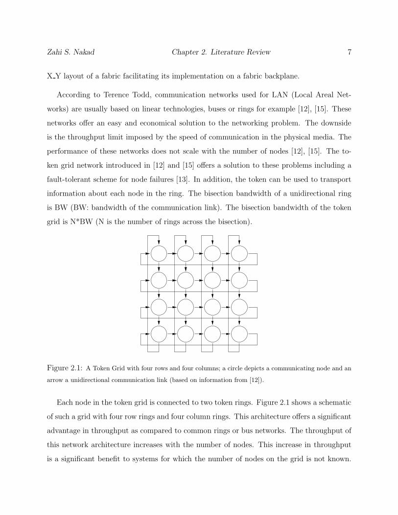
Figure 2.1: A Token Grid with four rows and four columns; a circle depicts a communicating node and an
arrow a unidirectional communication link (based on information from [12]).
Each node in the token grid is connected to two token rings. Figure 2.1 shows a schematic
of such a grid with four row rings and four column rings. This architecture offers a significant
advantage in throughput as compared to common rings or bus networks. The throughput of
this network architecture increases with the number of nodes. This increase in throughput
is a significant benefit to systems for which the number of nodes on the grid is not known.

Zahi S. Nakad Chapter 2. Literature Review 8
The physical aspect of this architecture maps well to the inherent X-Y nature of a fabric
weave.
The network interface of each node on this network has two configurations as shown in
Figure 2.2. In the DR (Double Ring) configuration (see Figure 2.2 (a)), the rings converging
at this node are separate. The second configuration is the SR (Single Ring) configuration,
shown in Figure 2.2 (b), in which the rings converging at this node are merged and operate
as a single ring. Special tokens are released in such a situation; Figure 2.3 shows the same
network with two rings merged at Node (1,2).
Full connectivity can be maintained in this network when faults occur. The condition to
establish this connectivity is that the network interface of each node can be configured to
remain in either the DR or SR state upon failure. The state to be mapped upon failure is
determined based on a failure-backbone; a specific node is configured to the SR state upon
failure if it belongs to the failure-backbone or to the DR state otherwise. If a node of the
failure-backbone detects a failure on its row, it forces itself into an SR state. This scheme
offers a slowly degrading performance upon failure while keeping full connectivity in the
network [13], [14]. This strategy only deals with failures of the node, not the link. The other
assumption is that the network interface of the failed node still forwards the packets in its
permanent DR or SR state. The following example shown in Figure 2.4, derived from [13],
will illustrate this feature:
b) Single Ringa) Double Ring
Figure 2.2: Communication through a node can be configured as a Double Ring or a Single Ring (based
on information from [12]).

Zahi S. Nakad Chapter 2. Literature Review 9
(0,0) (0,1) (0,2) (0,3)
(1,0) (1,1) (1,2)
Figure 2.3: Row 1 and Column 2 of this Token Grid are merged at node (1,2) (based on information
from [12]).
1. Column 0 is assumed to be the failure backbone.
2. Node 0,0 fails and is “fused” into the SR state.
3. Node 3,3 fails and is “fused” into the DR state.
4. The failure on node (3,3) forces node (3,0) into the SR state.
5. The result is a permanent ring spanning row 0, column 0, and row 3.
2.2 System Simulation
Building a separate prototype to conform to every decision point or aspect of the project is
extremely time consuming, raising the need to simulate the system, test several options, and
only implement the best result.
Creating a simulation environment is a complex and large undertaking, thus the decision
to use already existing simulation environments. Opnet [17] and Ptolemy [18], [19] will serve
as the simulation environments. The communication scheme between processing nodes on

Zahi S. Nakad Chapter 2. Literature Review 10
(0,0)
(3,3)(3,0)
Figure 2.4: Column 0 is the “failure backbone,” Nodes (0,0) and (3,3) have failed and are fused into the
SR and DR configurations respectively. Node (3,0) forces itself into an SR state (based on information
from [13]).
a computational fabric can be simulated in both environments. The entire operation of the
system, from the sensor behavior to the processing done on the nodes, can be simulated with
Ptolemy, thus covering all the significant aspects of the system.
2.2.1 Simulation Using Ptolemy
Ptolemy provides a heterogeneous simulation environment targeted to the simulation of
embedded systems; Ptolemy can represent systems that mix different technologies and de-
vices [19]. Ptolemy imposes some structure on the simulated systems. The components
simulated have to be encapsulated in Ptolemy actors. The interactions of components are
controlled by a “model of computation,” with several models provided. The best suited for
the system at hand has to be picked before the simulation is created. The different models
deal differently with time and concurrency. A list of nine different models of computations
are provided in [19] with a description of each model. These models are: Communication
Sequential Processes (CSP), Continuous Time (CT), Discrete Events (DE), Distributed Dis-
crete Events (DDE), Discrete Time (DT), Finite-State Machines (FSM), Process Networks

Zahi S. Nakad Chapter 2. Literature Review 11
angle
Line of bearing
Figure 2.5: Acoustic beamforming is used to determine the Line of Bearing of a noise source.
(PN), Synchronous Dataflow(SDF), Synchronous/Reactive (SR).
An e-textile system is constituted from different interacting components ranging from
complex processing nodes to simple acoustic sensors. The high-level simulation and the
inclusion of multiple interacting systems in the Ptolemy simulation environment map directly
to such a computational system. All of the components placed on the fabric can be simulated
as actors and their interactions as one of the models of computation. Significant aspects of
the physical world can be added to the simulation; for example, the sound of a passing large
vehicle.
2.3 Acoustic Beamforming
The e-textile prototype reports the line of bearing of large vehicles. To accomplish this,
acoustic beamforming is used to determine the direction of an incoming noise source as
shown in Figure 2.5.
Acoustic beamforming has been used in [20] to locate the source of the speaker for hands-
free telephony, and in [21] in a wearable computer system to determine if the speaker is the

Zahi S. Nakad Chapter 2. Literature Review 12
user or a person in conversation, differentiating between commands and regular speech. The
same principle was used in [22] for sound pickup in teleconference systems.
A low power beamforming algorithm compatible with integer mathematics has been re-
ported in [11]. This algorithm allows changing several variables to vary the accuracy and the
power consumption of the implementation. This variation permits different running options
and enables testing the trade-off between power and accuracy. The variables are: the number
of microphones used to collect the acoustic data, the number of acoustic samples collected,
and the number of search angles tested to decide the L.O.B. (Line Of Bearing) of the noise
source.
The process used in obtaining the L.O.B. is the following: the signals received at the
microphones are time shifted to account for an assumed location of the sound source, these
signals are then added and the values recorded; this process is repeated for a predefined
number of search angles. The power of the summed signals will increase as the assumed
search angle is closer to the L.O.B. and thus the search angle with the most resultant power
will be reported as the L.O.B. [11].
The principle of acoustic beamforming can be used to determine the distance between
two separate acoustic receivers. The maximum distance between the receivers allowed is the
wavelength of the sensed signal. The amount needed to shift one of the signals to get both
signals in phase is equivalent to the distance between them. This process is used to find the
distance between separate components.
2.4 Computational Fabric Research
The increasing attention paid to computational fabrics is boosting the research done in
this area. Emerging practical and useful implementations are helping in this advancement.
Industrial and academic research will be discussed in the following subsection.
Zahi S. Nakad Chapter 2. Literature Review 13
2.4.1 Pressure Sensing Fabric
ElekSen has developed a soft sensing fabric capable of interfacing to a multitude of devices.
ElekTex, the technology released by ElekSen, is a “soft sensing and switching system” that
provides digital signals to different devices based on impulses sensed by the fabric [23].
ElekTex thus acts as a smart and durable interface to already extant technology. Some of
the off-the-shelf items utilizing this technology reported by ElekSen are the ElekTex keyboard
and the Soft cell phone. The fabric in the phone acts as both the input interface and the
case.
The fabric can be designed to interact with different components to form a system with
a soft interface. The fabric is formed from regular and conductive fiber; the conductive fiber
can be made to detect separate areas on the fabric, buttons for example, of “about any
size [24],” other than sensing the X-Y position with a possible resolution of up to 1mm2.
A Z dimension sensing can also be accomplished where the third dimension is the strength
of the pressure exerted. Durability testing on the fabric simulated high pressures, folding,
tumbling, and tugging, after which the fabric (keyboard in this case) emerged with no faults.
The details of the test are available in [23].
2.4.2 Conductive Fiber
Electrical connections in any computational system are a must. With e-textiles, single strand
wires can be woven into the fabric, but such wires are not as malleable as natural fiber
or as discreet. Conductive fiber available in the market is mostly based on electro-static
dissipation needs; the conductivity of this fiber is not great enough to replace regular wire.
Conductrol [25] and Guilford Technical Textiles [26] are two examples of companies providing
such fibers.
Some research projects have been successful with the use of conductive fibers in their
systems. Metallic organza has been used in both the row and column fabric keyboard [4]
Zahi S. Nakad Chapter 2. Literature Review 14
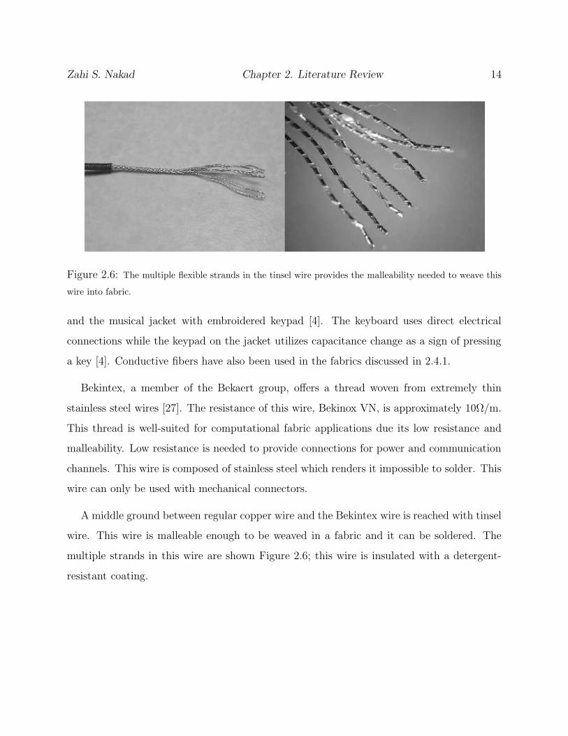
Figure 2.6: The multiple flexible strands in the tinsel wire provides the malleability needed to weave this
wire into fabric.
and the musical jacket with embroidered keypad [4]. The keyboard uses direct electrical
connections while the keypad on the jacket utilizes capacitance change as a sign of pressing
a key [4]. Conductive fibers have also been used in the fabrics discussed in 2.4.1.
Bekintex, a member of the Bekaert group, offers a thread woven from extremely thin
stainless steel wires [27]. The resistance of this wire, Bekinox VN, is approximately 10Ω/m.
This thread is well-suited for computational fabric applications due its low resistance and
malleability. Low resistance is needed to provide connections for power and communication
channels. This wire is composed of stainless steel which renders it impossible to solder. This
wire can only be used with mechanical connectors.
A middle ground between regular copper wire and the Bekintex wire is reached with tinsel
wire. This wire is malleable enough to be weaved in a fabric and it can be soldered. The
multiple strands in this wire are shown Figure 2.6; this wire is insulated with a detergent-
resistant coating.

Zahi S. Nakad Chapter 2. Literature Review 15
2.4.3 Wearable Computing and Computational Fabrics
Wearable computers promise to provide unobtrusive computing to the user, but to date
most wearable computers are bulky and cumbersome. Most users would not appreciate the
need to carry a backpack or components with significant bulk. Recent research has been
addressing these needs [28], [29], [30], [31], [32].
In the following sections, the computer system is separated into the areas of, input, output,
processing, power, and sensing devices, to allow for examination of e-textile progress in each
area.
2.4.3.1 Direct Input Devices
Many research efforts have been directed at making the direct input from the user less obtru-
sive and more conformant to regular life activities. Some of the efforts focus on discarding
the need for the input device to be held. Sensing the movement of the fingers is one promising
research direction; examples of such research projects are:
- Lightglove: this system detects the motion of the fingers by sensing reflectance off
the fingers of optical beams sent and received by photosensitive elements located in a
wristband [28].
- The active dressware research utilizes conductive polymers made to sense the hand
and finger movements when worn as a glove [29].
- Combining two mice (track-balls); each trackball controls a pie-shaped input and the
combination of the inputs of both trackballs operates as an input device [30].
- A glove input device was created in the Configurable Computing Lab at Virginia
Tech with the use of piezoelectric material. The study of the use of the piezoelectric
sensors in combination with fabrics in this device is closely related to this dissertation’s
research [32].
Zahi S. Nakad Chapter 2. Literature Review 16
These examples show the direction of research in making wearable computers less obtru-
sive. The use of computational fabrics in incorporating the sensors needed to sense such
inputs and the wires needed to send the signals to the processing node can be of great help
in increasing the wearability of the system and making it less obtrusive.
The keyboard approach as an input interface can also benefit from e-textiles. The ElekTex
keyboard is an example along with the GesturePad [31]. These keyboards can be hidden
inside the fabric with conductive thread sending the output to the processing node.
2.4.3.2 Interconnections Between the Separate Components
Computational fabrics can offer a communication medium using conductive fiber in the
textile of the garment. This type of connection will be invisible to the outside world and
more comfortable to the user. This will replace the use of regular wire as used in the
MIThril [33].
The Georgia Tech Wearable Motherboard (GTWM) [34] is an example of a system in
which the interconnections are inherent in the fabric. This system is to be used in a combat
situation to assess the seriousness of a soldier’s wound and communicate this data. The
interconnections in this fabric will detect if a bullet hit the user and determine the location
of the penetration. The system offers connections to other discreet components that can
monitor vital signs including heart rate and blood pressure. This system is to be worn as an
undergarment to offer minimal interference with the soldier’s operation.
The GTWM can be used as a PAN (Personal Area Network) where the devices carried
by the user can interact and share data [6]. The closeness of the devices to the user in such
a system allows the use of sensors in the fabric to learn “habits” of the user and thus to
react in different ways to different user situations, which is discussed in further detail in
Section 2.4.3.5.

Zahi S. Nakad Chapter 2. Literature Review 17
2.4.3.3 Processing Device
The use of computational fabrics with the processing elements is limited to providing connec-
tions to the other devices in the system. The creation of switching elements in the distant
future in fiber format can provide the basis of creating fabric processing elements. The
Macroelectronics Group at Princeton University is working on creating macroelectronics,
integrated circuits made by thin film techniques. Macroelectronics are larger than semicon-
ductor wafers but they will be flexible and rugged [35].
2.4.3.4 Power Device
Wearable computing can be considered a direct application of e-textiles. Bulky battery
packs will not fit the e-textiles objectives in creating a ubiquitous system. The following
section will provide an overview of some power cell products provided in a thin package.
Ultralife [36] 1mm battery packs; Infinite Power Solutions provide a film form battery, the
LiTE*STAR. The LiTE*STAR is an extremely thin battery with a great cycle life and an
all solid-state construction [37].
The development of fiber-form batteries would be extremely helpful in decreasing the
bulk in a wearable system. This fabric would be incorporated seamlessly in the e-textile.
Textile batteries are being studied at NCSU [38]. The electrochemical synthesis of conductive
polymers is reported in [8]. Currently off-the-shelf products are offered as thin batteries from
Ultralife [36] for example or film solar cells from Iowa Thin Films [39].
2.4.3.5 Context Awareness
The operation and application of a wearable computer should vary based upon its surround-
ings. The response to certain actions of the user, gestures for example, should be different
depending on the present location/setting of the user [40]. Context awareness depends
greatly on the ability of the computer system to sense the surrounding environment. In

Zahi S. Nakad Chapter 2. Literature Review 18
Warp
Weft
Reed
Batten
Shed Rod
Figure 2.7: The basic loom used in creating the prototypes for this research.
an e-textile application, the sensors (acoustic, motion, video, etc.) will be attached to the
fabric and the communication will be provided through the fabric to the processing node.
The e-textile can offer the routing capabilities required; the relevant sensors will be queried
when the processing node requires data from all the sensors “facing forward,” for example.
Computational fabrics will enhance this research area in wearable computing by offering
the ability to distribute sensors over the fabric. Different types of sensors can be incorpo-
rated at the same time. The system will be able to adapt to different situations with added
fault-tolerance. A Sensor Jacket is reported in [41]; this jacket can detect the posture and
movement of the wearer with the use of knitted stretch sensors. Machine-learning techniques
were used to achieve 2% error in an in-door navigation application with the use of cheap
wearable sensors [42].

Zahi S. Nakad Chapter 2. Literature Review 19
2.5 Manufacturing Textiles
Hand looms for weaving textiles have existed for at least eight thousand years [43]. The
study of the ancient hand looms offers an understanding of the weaving process of fabrics.
The following description follows that of [43]. The first set of yarns used are stretched with
the use of hanging weights, the weight of the weaver, or between the ends of a fixed frame.
These yarns are called the warp yarns and after being stretched they are interlaced by the
weft or filling yarns. The filling yarns are pushed over and under the warp yarns, the sim-
plest scheme is going on top and below each stretched warp yarn. Figure 2.7 shows the basic
parts of a loom.The filling yarns can be fed with the use of a shuttle carrying a bobbin that
provides the yarn that needs to be interlaced. Some modern looms use shuttles but faster
looms use other mechanisms that shoot the yarn through separated warp yarns [43]. To pack
in the newly added weft yarn, a comb-like structure, the reed, is used to push the filling yarn
in place. The reed is mounted on a frame, the batten, that helps in pushing the reed and
keeping it steady; the batten is used in the automated looms. Moving the shuttle through a
separated set of yarns is easier and faster than going over and under each individual warp
thread. The shed rod or heddles are used to lift specific warp yarns from the level of their
neighbors and ease the introduction of the filling yarn. This is a simplified description of the
process of weaving which has advanced to increasingly complex looms and techniques but is
sufficient for understanding the shape and creation of fabrics for our purpose. Visualizing
the process of weaving can help in understanding some of the design decisions we took. The
preceding was a short summary of the information provided in [43]. In the designing process,
the wires in the warp, as the weaving starts, are permanent, while changes in the weft wires
can be made during the weaving.
Chapter 3
Exploring the e-Textile Architecture
The advancement of the textile industry has resulted in a high level of automation along
with relatively cheap process of manufacturing. Textiles offer a useful form factor for new
electronic technology applications. The formation of a platform for deploying the sensing
and processing elements required in a wearable computing system without the use of external
wires is much needed. The fabrication of large textiles offers the environment needed for
deploying the components for large scale systems. Research initiatives in using electronic
textiles as a platform for pervasive computing is presented in [44].
This chapter explores the e-textiles domain. The issues faced will be described along with
the temporary or permanent solutions used. Several projects under study will be introduced.
3.1 Motivations for e-Textiles?
The first question asked is, why e-textiles? The following section describes the benefits
expected from the e-textile architecture.
20

Zahi S. Nakad Chapter 3. Exploring the e-Textile Architecture 21
3.1.1 Cheap and Large-Area Backplane
Fully automated and large-scale industrial looms make it affordable and easy to create large-
area textiles [1]. The textiles are fabricated economically and with precise control. This
technology acts as a basis for the e-textile architecture.
Applications requiring large-area systems will benefit greatly from the combination of
electronic components and these textiles. This combination will create a backplane to be
tailored to economically fit the requirements of each specific application. Other textile prop-
erties, flexibility for example, can add to the benefits of such a new architecture. Surrounding
a solid object, vehicle, or building, with sensors is easily done by draping the object with a
textile “sprinkled” with the required sensors.
3.1.2 Ease of Deployment
E-textile systems are easily deployable, especially for large scale applications. The system
can be rolled up into bundles and spread out in the field. In military applications, an enemy-
monitoring system can be deployed in a parachute; the fabric of the parachute would be the
active element of the system, while the object attached can be just a decoy. User operation
in confined areas, e.g., maintenance work on an airplane, can be made easier by the use of
wearable e-textile systems to incorporate the equipment and plans needed.
3.1.3 Concealment and Comfort
Integrating the components and their connections into the fabric that constitutes the back-
plane of the system can be extremely beneficial. In wearable computing systems, unobtru-
siveness is highly appreciated along with concealment from the outside world. Concealment
is also needed in large area systems, particularly for military and ubiquitous computing ap-
plications. With more advanced fiber [23], [27], [38], [8] and packaging technologies [45],
Zahi S. Nakad Chapter 3. Exploring the e-Textile Architecture 22
e-textile systems can be made invisible to the outside world.
3.1.4 Fault-Tolerance
Any tear in the fabric can result in severing connection lines, thus the need for implement-
ing alternative communication routes. The manufacturing process and operation in hostile
territories can introduce tears in the fabric (communication and power disruption). Destruc-
tion of computational nodes and sensors are other faults that can occur during operation.
The fabric does offer a less fragile environment than just spreading wires between different
components, but is perhaps not as robust to physical faults as a wireless network.
The low cost and the form factor of e-textile systems make it easy to incorporate re-
dundancy into the system. Attaching redundant components does not use up expensive
real-estate and extra communication routes can be easily added by exchanging a regular
thread with a conducting one.
3.1.5 Power Consumption
E-Textiles can act as an alternative to wireless personal area networks. In such applications,
e-textiles offer a reduction in component cost and in power consumption. The savings are
derived from a reduction in the number of communicating modules and in the inherently
cheaper wired communication. A methodology for quantifying such savings was presented
in [46], which showed at least a factor of 14 savings in energy consumption by using an
e-textile implementation rather than a full wireless one.

Zahi S. Nakad Chapter 3. Exploring the e-Textile Architecture 23
3.2 Implementation Issues
E-Textiles are relatively new and thus lack the support of off-the-shelf products or reliable
processes. The following section will discuss some of the issues encountered in implementing
applications on e-textile architectures.
3.2.1 Embroidery or Weaving
E-Textiles offer inherent electrical connections for power and data in the fabric, but the
issue of how to integrate conductive fibers must be addressed. The first idea explored was
embroidery machines. The use of embroidery machines would follow directly from PCB
(Printed Circuit Board) design; the circuit for the interconnections would be drawn and
a direct mapping done to create the system. Embroidery machines from Bernina [47] and
Brother [48] are controlled by computers, with the user providing a digital image of the
embroidery. With the use of conducting thread or wire, this process becomes the direct
translation of the PCB design in the e-textiles world.
The researchers in [4] were able to embroider successfully for their needs using silk-organza.
The high resistance of silk-organza, however, makes data and power transmission difficult.
The trials at the Virginia Tech Configurable Computing Lab on standard wires fouled the
embroidery equipment. In addition, embroidery is considered to be a fairly expensive process
in the textile business.
Another option for integrating the wires is weaving. The first advantage of weaving is the
seamless integration of the process in large looms, by replacing some threads with conductive
wires. Stainless steel wire from Bekintex [27] or tinsel wire can easily replace thread in the
loom; both wires were integrated in e-textile prototypes in the lab. Unlike embroidery, the
insertion of the wires is done at the time of weaving the textile and is not nearly as flexible
in terms of thread positioning.
Zahi S. Nakad Chapter 3. Exploring the e-Textile Architecture 24
With the weaving option, two types of implementations have been explored. The first is a
multiple layer textile that uses an insulating layer, allowing uninsulated conductive threads
to be used in different layers with the connections between different layers done mechanically
by crossing through the insulating layer. The other option is a one layer solution, where at
least one of the directions of the wires, warp or weft, has to insulated. Electric connections
are more difficult because the insulation at the connection point has to be removed. On the
other hand, the one layer option is less bulky, less expensive to make, and avoids possible
inadvertent shorts.
3.2.2 Connections and Attachments
The integration of components into the fabric is a driving force behind the e-textile archi-
tecture. The components to be integrated vary greatly depending on the application. The
perfect situation for e-textiles would be to have all the components in fiber form: fiber micro-
phones, batteries, etc. The fiber form components are integrated into the system in the same
manner as the conductive threads. The electrical connection needed for these components
can be made using solder. Other techniques, utilizing mechanical connectors for example,
are under investigation.
Other components will be attached to the fabric in their discrete, off-the-shelf form. The
number of pins to be attached is important and affects the decision on the type of attachment.
Some components, e.g. microphones, require minimal connections. These components can
be attached directly to the conductive threads with solder or a mechanical connector.
Higher-density components, primarily ICs, require a very tight connecting mesh of lines
made possible by PCB boards. Connecting all of these pins directly to the fabric is impossible
at the present time. Thus an interface-pin-reducer is needed; for example, a regular PCB
board that takes care of connecting the needed ICs for a specific application. The ICs on this
board will create a node with minimal connections to the fabric. The node in the acoustic
beamformer is a perfect example and it was attached with mechanical means, 2-mm pin

Zahi S. Nakad Chapter 3. Exploring the e-Textile Architecture 25
Figure 3.1: 2mm header pin used to connect the board to the prototype fabric
header connectors (Figure 3.1), and solder. Recent technology [45] allows for the packaging
of this type of node into foldable layers, reducing their size significantly. This reduction in
size helps in meeting the promise of unobtrusive e-textiles.
The use of solder in our prototype with the 2-mm pin headers proved to be time consum-
ing and fragile. This type of connection does not render itself easy for mechanization, and
thus the process will be hard to automate to reach a production phase with e-textiles. The
proposed connecters will use mechanical means for connections, such as insulation displace-
ment. These connectors are generally formed of two clamping pieces that are easily aligned
and clamped in a mechanized fashion. The 3MTM ScotchLokTM Insulation Displacement
Connectors (IDCs) are examples of such connectors.
3.3 How to Explore?
Fully exploring a new and undeveloped architecture requires experimentation. Novel appli-
cations have been created to serve as an input to further the development of the architecture
Zahi S. Nakad Chapter 3. Exploring the e-Textile Architecture 26
and help in creating a set of guidelines to serve as the basis for future research in the area.
These guidelines and experiences helped in creating the simulation environment that serves
as an enhancer for the current projects and a drawing-board for new ideas.
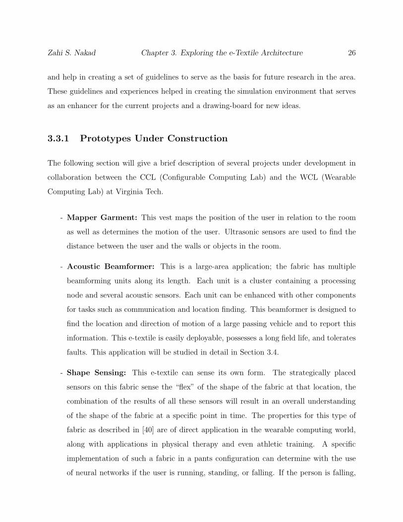
3.3.1 Prototypes Under Construction
The following section will give a brief description of several projects under development in
collaboration between the CCL (Configurable Computing Lab) and the WCL (Wearable
Computing Lab) at Virginia Tech.
- Mapper Garment: This vest maps the position of the user in relation to the room
as well as determines the motion of the user. Ultrasonic sensors are used to find the
distance between the user and the walls or objects in the room.
- Acoustic Beamformer: This is a large-area application; the fabric has multiple
beamforming units along its length. Each unit is a cluster containing a processing
node and several acoustic sensors. Each unit can be enhanced with other components
for tasks such as communication and location finding. This beamformer is designed to
find the location and direction of motion of a large passing vehicle and to report this
information. This e-textile is easily deployable, possesses a long field life, and tolerates
faults. This application will be studied in detail in Section 3.4.
- Shape Sensing: This e-textile can sense its own form. The strategically placed
sensors on this fabric sense the “flex” of the shape of the fabric at that location, the
combination of the results of all these sensors will result in an overall understanding
of the shape of the fabric at a specific point in time. The properties for this type of
fabric as described in [40] are of direct application in the wearable computing world,
along with applications in physical therapy and even athletic training. A specific
implementation of such a fabric in a pants configuration can determine with the use
of neural networks if the user is running, standing, or falling. If the person is falling,
Zahi S. Nakad Chapter 3. Exploring the e-Textile Architecture 27
the pants could order the deployment of an airbag. Examples of the sensors used are
accelerometers and piezo-electric sensors.
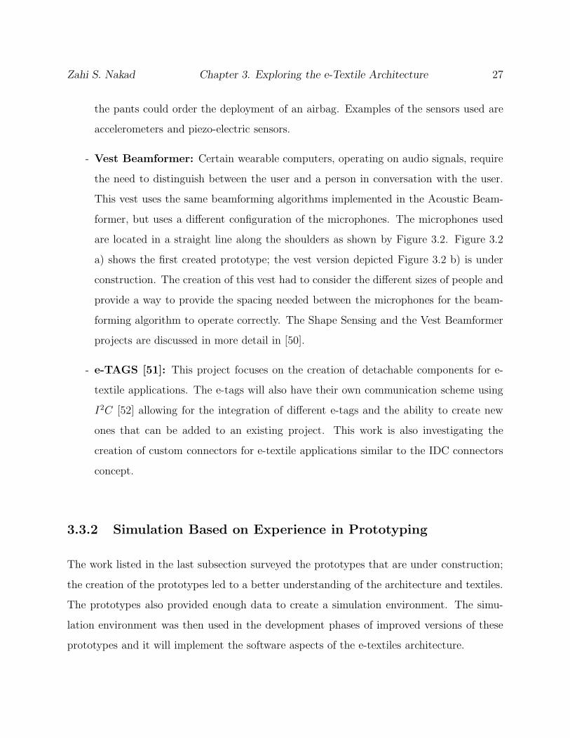
- Vest Beamformer: Certain wearable computers, operating on audio signals, require
the need to distinguish between the user and a person in conversation with the user.
This vest uses the same beamforming algorithms implemented in the Acoustic Beam-
former, but uses a different configuration of the microphones. The microphones used
are located in a straight line along the shoulders as shown by Figure 3.2. Figure 3.2
a) shows the first created prototype; the vest version depicted Figure 3.2 b) is under
construction. The creation of this vest had to consider the different sizes of people and
provide a way to provide the spacing needed between the microphones for the beam-
forming algorithm to operate correctly. The Shape Sensing and the Vest Beamformer
projects are discussed in more detail in [50].
- e-TAGS [51]: This project focuses on the creation of detachable components for e-
textile applications. The e-tags will also have their own communication scheme using
I2C [52] allowing for the integration of different e-tags and the ability to create new
ones that can be added to an existing project. This work is also investigating the
creation of custom connectors for e-textile applications similar to the IDC connectors
concept.
3.3.2 Simulation Based on Experience in Prototyping
The work listed in the last subsection surveyed the prototypes that are under construction;
the creation of the prototypes led to a better understanding of the architecture and textiles.
The prototypes also provided enough data to create a simulation environment. The simu-
lation environment was then used in the development phases of improved versions of these
prototypes and it will implement the software aspects of the e-textiles architecture.
Zahi S. Nakad Chapter 3. Exploring the e-Textile Architecture 28
Mics
(a) (b)
Figure 3.2: The Vest Beamformer is able to locate and distinguish between different audio sources.
The simulation environment provides designers with the means to explore the e-textiles
architecture space without resorting to the creation of physical prototypes. This environment
also helps in fine-tuning current designs to, for example, reach a better configuration in
terms of power consumption or accuracy of results [53], [54]. The design of the simulation
environment will be discussed in further detail in Chapter 5.
The process of the development of the e-textiles architecture based on the cycle presented
in Figure 3.3 can start at any node in the cycle. Staring with the creation of a concept,
depending on the complexity or ease of implementation we can move to either simulation or
physical testing and use the remaining step as verification. In the first developments, the
concept of the beamformer was the starting point, the hardware was then created for lack of
any other means, and last moved to creating the simulation environment. This environment
was then used to fine-tune the hardware. A new project would be started by the creation of
the concept, simulating the process, and finally physical implementation. In the same way,
during simulation, a new concept can be conceived, designed, and implemented in hardware.

Zahi S. Nakad Chapter 3. Exploring the e-Textile Architecture 29
Figure 3.3: The relationship between the theoretical concept, simulation, and prototyping follows the cycle
shown in both directions and at any starting point.
The same applies in a physical testing ⇒ concept design ⇒ simulation ⇒ physical testing
cycle.
3.4 Acoustic Beamformer Prototype
The following section discusses the implementation of the beamforming array. The architec-
tural nomenclature, node creation, component connection, and the prototype construction
will be presented. The software running in the processing nodes will be introduced.
3.4.1 Acoustic Beamforming Array
The implemented system collects acoustic data from several microphones, converts the analog
data to digital format, and runs a beamforming algorithm to determine the line of bearing of
a large vehicle. The computed value is communicated to peer systems or the outside world.
Operation in hostile territories requires the implementation of fault-tolerant schemes; for
example, this system is augmented with seven sensors when only three sensors are absolutely

Zahi S. Nakad Chapter 3. Exploring the e-Textile Architecture 30
of a commercially sold software package is permitted. © 2001, Carlo Kopp
Distribution of this artwork as part of the xfig package, where xfig is part
e−textileCluster 1 Cluster 2
Microphone
Node
Cluster
Target
Speaker
of a commercially sold software package is permitted. © 2001, Carlo KoppDistribution of this artwork as part of the xfig package, where xfig is part
Figure 3.4: A conceptual rendering of a computational fabric with two acoustic array clusters.
needed to provide the information needed for the beamformer [3]. The following definitions
will be used throughout the discussion. A node is the processing component, it is able
to gather information from the acoustic sensors, convert it to digital format, compute the
direction of the vehicle and communicate the result. A cluster includes the node and the
sensors directly connected to it. A cluster can operate as a stand-alone system and provide
useful information independently. An acoustic beamformer includes one or more clusters.
Such a system will benefit from the redundancy in fault-tolerant schemes and in improving
the computed result. The angle result computed at every cluster can be combined to provide
position data via triangulation. Figure 3.4 shows an abstract view of the introduced terms.
The fabric is the platform where the components of the system are deployed as shown in
Figure 3.5. The placement of the several components on the fabric initially deals with the
textiles as a planar structure. Figure 3.6 shows the plan used to implement the conductive
wires along with the positions of the components when the fabric is held in a plane. This

Zahi S. Nakad Chapter 3. Exploring the e-Textile Architecture 31
Figure 3.5: The implemented Acoustic Beamforming Array (one cluster) shown on a multi-layer fabric.
diagram was used to help the weaver in creating our fabric prototypes that resulted in the
acoustic beamformer.
In any stand-alone system, power is a major issue. Battery replacement is an impossibility
or a highly improbable luxury; thus, sensing operations on battlefields necessitates power
efficiency. The tasks implemented and the hardware operation should be power-aware; using
approximations and pushing the processors into dormant states. The software running on
the nodes in the implemented 30-foot fabric can force the hardware to a dormant state, the
node will wake up only when there is a significant acoustic signal. A node in this system
can also be awakened by another node in the system by sending a data packet.
3.4.2 Hardware and Software of the Processing Node
The hardware processing node in the acoustic beamformer was designed for this specific
project. The experience gained from its creation had a more general effect. The implemented
interrupt-driven software guided the simulation effort as will be discussed in Chapter 5. The

Zahi S. Nakad Chapter 3. Exploring the e-Textile Architecture 32
Figure 3.6: The textile schematic of the Acoustic Beamformer shown with one node and seven microphones
along with the conductive threads in the fabric.
hardware design provided significant experience in printed circuit board design, and mixed-
signal circuit design.
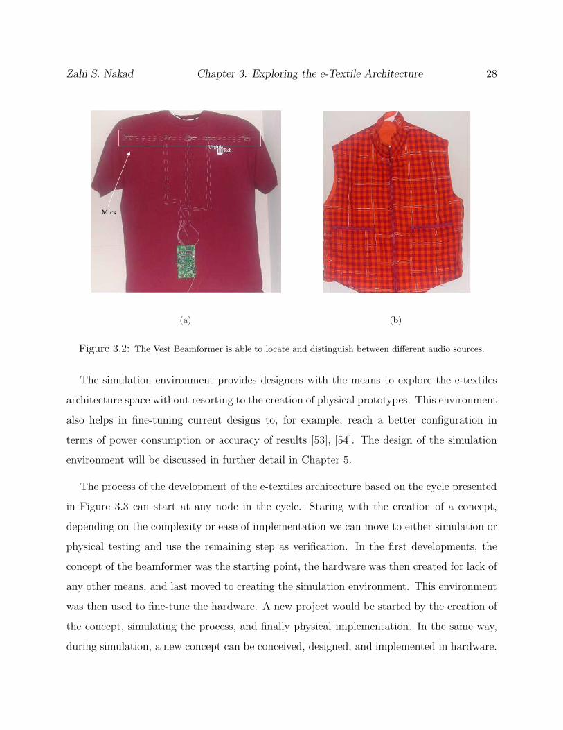
Figure 3.7 shows the block diagram of this node. The ADSP-2188 [55] is a low-power
fixed-point processor with enough memory space and interrupt handling capability to deal
with the acoustic data collection and the L.O.B formation. The board is also equipped with
a hardware wake-up scheme that sums the acoustic data and sends a wake-up signal to the
processor if a certain “loudness” threshold is crossed. The software running on the DSP
(Digital Signal Processor) is downloaded with the use of the flash memory, and the output
of the beamforming is communicated through a serial port.
The whole process on the board is controlled by a timer interrupt that acts as the lowest
granularity of events that can occur. This timer interrupt signals the A/D to acquire data and
this data is communicated to the DSP. Data transmission and reception from the A/D are
controlled by interrupts as all the other aspects of this software. Data acquisition continues
until a pre-determined buffer size is filled and the beamforming code is instantiated; the
results are then computed and communicated.
Zahi S. Nakad Chapter 3. Exploring the e-Textile Architecture 33
Ring 1
Op Amp
Op Amp
A/DDSP
2188M
Flash
Mic 1
Mic 2
Mic 3
Mic 4
Mic 5
Mic 6
Mic 7
2 3 GPS
Figure 3.7: The block diagram of a node shows the interface with the fabric along with the inner connections
Active_Message
SIGTIMER
SIGSPORT0RECV
SIGSPORT0XMIT
SIGSPORT1XMIT
SIGSPORT1RECV
SIGPWRDWN
SIGIRQE
Interrupt
Handler
Timer_Subroutine
Transmission_Subroutine
Serial_Port_Transmission_Subroutine
Serial_Port_Reception_Subroutine
PowerDown
Node_Reception_Subroutine
Timer_Mic_Sampling
Timer_Milli_Second
Timer_Send_To_Node
Timer_Receive_From_Node
Reception_Subroutine
Queue_Get_Message
Transmit
Send_To_Node
Receive_From_Node
Transmit_Result
Queue_Add_Message
Transmit_Request
Transmit_Result_Serial_Only
Data_Manipulation
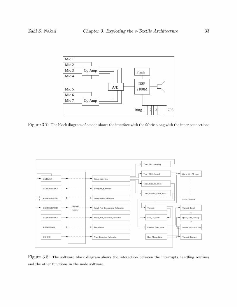
Figure 3.8: The software block diagram shows the interaction between the interrupts handling routines
and the other functions in the node software.

Zahi S. Nakad Chapter 3. Exploring the e-Textile Architecture 34
The DSP has two generic serial ports, one is used to communicate with the A/D and the
other with a host machine. Sending data between nodes is done with the help of flag pins;
every character to be sent is encoded in a fashion similar to RS-232. The flags send out their
values using the timer interrupt as a synchronization. The reception side is more complex.
Each incoming data line is tied to an interrupt and a data pin (RAM data pin). At the
reception of the first bit (forced to be a 1), the interrupt signals the reception of data and
is disabled until the end of the reception, and the DSP reads the data as if reading from its
memory. The memory reads are also synchronized with the timer interrupt. All nodes have
to run the timer interrupt at the same frequency. A more advanced node would use a DSP
with more communication ports to enable the use of I2C for example. Data packets are
controlled with the use of a general message queue. This queue stores all the packets that
need to be communicated and controls transmission in a FIFO (first-in first-out) fashion.
Figure 3.8 depicts all the interacting parts of the software including the interrupt handlers. A
specific path in this diagram will be scrutinized in detail in Chapter 5 to show the operation
of the simulator alongside the operation of the hardware.
Chapter 4
Electronic Textile Architecture
The work described in Chapter 3 provided the input to create the basis of the Electronic
Textile Architecture. This architecture will derive its precepts from the previous experiences
and show possibilities for future directions. These directions will later be either positively
proved as precepts or negatively dismissed as were previous attempts. This section will
provide an overview of the created precepts and the discarded attempts in relation to tasks
in the creation and implementation of an electronic textile system.
4.1 Embedding of Conductive Channels
An electronic textile is defined as a set of sensors, processors, and actuators embedded in a
fabric backplane interacting to serve a specific goal, with all communication and power lines
integrated in the fabric. The integration of the communication and power lines is integral to
the architecture. This section will discuss the discarded attempts, precepts, and open issues
of the architecture.
35
Zahi S. Nakad Chapter 4. Electronic Textile Architecture 36
4.1.1 Embroidery vs. Weaving
Using weaving as the method for incorporating conductive channels in an electronic textile
was discussed in detail in Section 3.2.1. The conclusions from our experience are:
- Precept: Weaving will be used to incorporate conductive channels. The locations
of these channels will be determined at the outset of the weaving process. Weaving
dictates an X-Y structure in the network.
- Attempt: Embroidery did not prove successful for the type of conductive elements
we are using in this architecture. The embroidery machines were jammed by the used
conductive channels.
4.1.2 Uninsulated vs Insulated Conductors
The choice between insulated and uninsulated wire or conductive channel (will be referred
to as wires until the end of the section) has a great impact on the direction and the design
decisions to be taken. Uninsulated wires provide ease of connection but at a cost. In our
implementation of a beamforming cluster using uninsulated wires we implemented the fabric
in multiple layers; two layers carrying wires either along the length or width of the fabric
and an insulation layer between them. The connection between wires on separate layers goes
through the insulation layer and is fixed mechanically. This type of connection proved to
be unstable. The uninsulated wires provided short circuit risks if the fabric is subjected to
crumpling. Another problem with uninsulated stranded wire is the “fraying” of the strands
as these wires undergo the weaving process in a loom, creating the potential for short circuits.
The use of insulated wires provides the ability to use single layer fabrics, much simpler to
manufacture, but there is the issue of removing the insulation when a connection is needed.
The method of connecting to these wires will be discussed in Section 4.2.1.
- Precept: Use insulated wires to simplify the manufacturing of the fabric while devising
Zahi S. Nakad Chapter 4. Electronic Textile Architecture 37
better wire connection techniques.
- Attempt: Use of uninsulated wires was not successful for the above mentioned reasons.
4.1.3 Conductive Material
The different types of wires in an electronic textile has been discussed in detail in Sec-
tion 3.2.1. The conclusions are as follows:
- Precept: The properties of the tinsel wire combines flexibility, conductivity, and sol-
derability. The insulation on these wires is detergent resistant and thus can withstand
cleaning the fabric.
- Attempt: Single strand wire did not provide the needed flexibility and at high gauges
it was susceptible to breakages. The Bekintex wire has a tendency to “fray” which can
introduce short circuits.
- Open Issues: More research and experimentation is required on the use of conductive
polymers to determine their utility in carrying power, analog data, and digital data.
4.1.4 Analog vs Digital Signals
The question of sending analog or digital signals on the wires is application dependent, but
there are aspects that can be generalized. Analog transmission is more prone to noise and
interference, but we were successful with the acoustic beamformer due to the low sampling
rates and the low communication speeds on other lines in the fabric. Interference will have
a higher impact in a motion sensing vest, for example, that incorporates cameras and/or
antennas.
Using digital communication for all the signals on an electronic textile will provide a more
stable system, along with pushing analog processing of the data closer to the sensors. The
Zahi S. Nakad Chapter 4. Electronic Textile Architecture 38
processing nodes will only receive digital signals in this setup. Using I2C, for example, for
all signal communications eases the general design of the system. When a specific standard
is tested and then used for all consequent applications, the number of variables in a system
is reduced. For example I2C forces the use of four wires for any communication channel,
thus any channel in the fabric should consist of four wires throughout. Digital transmission,
on the other hand, adds the cost of analog/digital conversion and communication hardware
to each sensor.
- Precept: Digital transmission should be used for all of the signals on such a system.
- Attempt: Analog transmission can also be used, but is not recommended.
4.1.5 Communication Busses
Following the previous discussion, digital signals will be used throughout an electronic textile
system. The use of I2C busses throughout helps in standardizing the layout of the fabric as
can be seen in Figure 4.1 which represents a unit of the fabric used in creating the textile
component of the Shape Sensing project [50]. The wires are implemented in sets of four
to carry all the signals of the busses, and these busses are repeated to generalize the fabric
created and to provide support for future endevours using the same fabric. The fabric used in
the Acoustic Beamformer was specifically designed for that project and cannot be configured
for other implementations.
- Precept: Use a standard bus communication method for all signals in the fabric to
help in generalizing the fabric design.
- Attempt: Design the fabric for the specific application results in a loss of re-usability.

Zahi S. Nakad Chapter 4. Electronic Textile Architecture 39
Figure 4.1: Schematic of a unit of fabric of the textile used in creating the shape sensing pants [56].
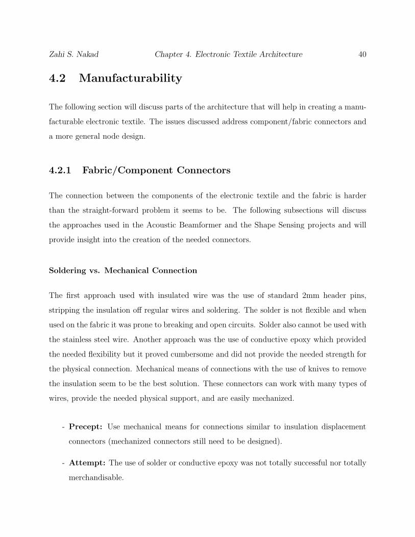
Zahi S. Nakad Chapter 4. Electronic Textile Architecture 40
4.2 Manufacturability
The following section will discuss parts of the architecture that will help in creating a manu-
facturable electronic textile. The issues discussed address component/fabric connectors and
a more general node design.
4.2.1 Fabric/Component Connectors
The connection between the components of the electronic textile and the fabric is harder
than the straight-forward problem it seems to be. The following subsections will discuss
the approaches used in the Acoustic Beamformer and the Shape Sensing projects and will
provide insight into the creation of the needed connectors.
Soldering vs. Mechanical Connection
The first approach used with insulated wire was the use of standard 2mm header pins,
stripping the insulation off regular wires and soldering. The solder is not flexible and when
used on the fabric it was prone to breaking and open circuits. Solder also cannot be used with
the stainless steel wire. Another approach was the use of conductive epoxy which provided
the needed flexibility but it proved cumbersome and did not provide the needed strength for
the physical connection. Mechanical means of connections with the use of knives to remove
the insulation seem to be the best solution. These connectors can work with many types of
wires, provide the needed physical support, and are easily mechanized.
- Precept: Use mechanical means for connections similar to insulation displacement
connectors (mechanized connectors still need to be designed).
- Attempt: The use of solder or conductive epoxy was not totally successful nor totally
merchandisable.
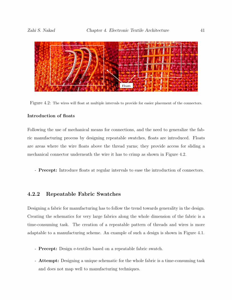
Zahi S. Nakad Chapter 4. Electronic Textile Architecture 41
Floats
Figure 4.2: The wires will float at multiple intervals to provide for easier placement of the connectors.
Introduction of floats
Following the use of mechanical means for connections, and the need to generalize the fab-
ric manufacturing process by designing repeatable swatches, floats are introduced. Floats
are areas where the wire floats above the thread yarns; they provide access for sliding a
mechanical connector underneath the wire it has to crimp as shown in Figure 4.2.
- Precept: Introduce floats at regular intervals to ease the introduction of connectors.
4.2.2 Repeatable Fabric Swatches
Designing a fabric for manufacturing has to follow the trend towards generality in the design.
Creating the schematics for very large fabrics along the whole dimension of the fabric is a
time-consuming task. The creation of a repeatable pattern of threads and wires is more
adaptable to a manufacturing scheme. An example of such a design is shown in Figure 4.1.
- Precept: Design e-textiles based on a repeatable fabric swatch.
- Attempt: Designing a unique schematic for the whole fabric is a time-consuming task
and does not map well to manufacturing techniques.

Zahi S. Nakad Chapter 4. Electronic Textile Architecture 42
4.2.3 Smaller More General Nodes (Beamformer vs e-TAGS)
The design direction of sending all signals on digital busses spread in a regular pattern over
the textile pushes the design space into the creation of more general processing nodes. There
will be a need for sensor data processors that will convert the analog data and provide the
communication interface. The generalization of these nodes will lead to the manufacturing
of “sensor nodes” that can be tuned to the specific sensor. This path diverts from the
first approach of designing a specific node for a specific job as was done with the Acoustic
Beamformer. The same concept can be applied to the processing nodes. The creation of
the more general nodes will decrease the price of manufacturing and designing by using a
mass production approach, and will map better to the approach of standardizing all signal
transmissions on these systems. This approach is under research in the e-TAGS project [51].
- Precept: Move to generalizing the nodes in the electronic textile.
- Attempt: The creation of specific nodes for specific jobs is too expensive.
4.2.4 Classes of Nodes
With the development of the electronic textile architecture and technology, two classes of
nodes will arise. Sensor nodes that use simple microcontrollers will become smaller and will
ultimately be integrated in the fabric. Communication hubs and processing nodes will get
more powerful with technology advances.
- Precept: The architecture can be used to develop applications that will map to pre-
dicted technology advances and to the different classes of nodes.
Zahi S. Nakad Chapter 4. Electronic Textile Architecture 43
4.3 Software
This section will provide the aspects of the software part of the the architecture. These
aspects are provided in the simulation environment. The implementation in the software
environment forces the simulated processes to follow these precepts by using the provided
services.
4.3.1 Interrupt Driven Processing
An electronic textile system will most probably deal with sensing certain physical phenomena
and react according to pre-determined procedures. Interrupt driven processing maps directly
to such a situation; a processor will not process unless it receives data (interrupt event),
sensor nodes will not report unless there is a significant action (interrupt event) and so
forth. The simulator provides a core simulator of a processor that is able to process interrupts
and respond accordingly. The simulated operation of the system can easily be moved to a
hardware installation with an interrupt driven processor. This applies to the ADSP-2188
used in the Acoustic Beamformer and the microcontrollers used in the e-TAGS.
- Precept: Interrupt driven processing maps to the hardware process and the sensed
phenomena and thus will be the processing model used in the architecture.
4.3.2 Fault-Tolerant Communication Scheme
The use of electronic textile systems in harsh environments will introduce faults in the system.
Such a stand-alone system should be able to withstand such faults and continue operation
perhaps with decreased functionality. The electronic textile architecture will provide a fault-
tolerant communication scheme that will route around faults. The network will be discussed
in great detail in Chapter 6. The provided network will also map to the X-Y topology of a
weave and provide the support for “sleeping” nodes.
Zahi S. Nakad Chapter 4. Electronic Textile Architecture 44
- Precept: Provide a communication scheme that maps to the geometry of the weave
and provides a fault-tolerant scheme.
4.3.3 Human Motion Databases for Prototyping
The electronic textile architecture provides the ability to simulate a textile. For wearable
systems, this architecture will provide the ability to test the design on a large number of
people through the use of human motion databases available from [57], for example. An
operational testing phase follows the creation of a prototype. The results of these tests
are more credible because of the large number of test subjects. This architecture provides
means for testing an e-textile prototype by using these human motion databases and thus
providing access to a large number of test subjects to verify the operation of the prototype
or its concept.
- Precept: Use a larger number of subjects to better test the prototype during both
the conception and development stages.
- Attempt: The lack of ability to test a system before it is created in hardware can
prove to be expensive, and testing on a small population can present misleading or
biased results.
4.3.4 Component Distance Finding
The shape of an electronic textile system can change during its operation, thus causing the
distances between the components in the system to vary. The importance of this variation
is application dependent. The hardware implementation of the distance finding process was
achieved. The full integration into the architecture will be accomplished at a later stage for
the specific applications.

Zahi S. Nakad Chapter 4. Electronic Textile Architecture 45
- Precept: Integration of distance finding capabilities into the electronic textile ar-
chitecture will be done for applications where it is crucially required. The current
prototypes have not required these capabilities.
The electronic textile architecture provides a structure and a path to be followed by
new prototype endeavors. This architecture also provides a simulation environment to test
concepts and improve extant hardware applications. A direction towards generality in the
design to reach a more manufacturable technology is also conveyed; the weave design should
allow for the creation of multiple sizes and types for different applications. Using a standard
communication scheme, for example, will help in simplifying the hardware nodes and the
communication portion of the design.

Chapter 5
Simulation
Our goal is to create an e-textile architecture that is accessible to future researchers. At
the outset of a project, implementing every aspect of an e-textile system in hardware can
be expensive and time consuming. Creating a software environment that simulates the
operation of e-textile systems can be extremely beneficial by allowing the design space to be
explored without having to build a prototype. Such a simulation environment can be used
to enhance the performance of extant systems as well.
Writing a simulation package from scratch is a major task and thus we decided to use
an available one. Ptolemy [19] was chosen because it is designed to simulate heterogeneous
and embedded systems. The created environment will be discussed by showing its operation
in regards to the system described in Section 3.4. This chapter will describe the different
aspects of the simulator and will demonstrate its general usability, Section 5.1. With Ptolemy
we are able to simulate the interaction with the outside world and the response created
from the e-textile system. This chapter will discuss the simulation of the acoustic signals
created by a large vehicle at a specific location with respect to each microphone, Section 5.2.
The discussion will also cover the simulation of computing the result of the beamformer
code, Section 5.3 along with the operation of this code while communicating with other
nodes in the system Section 5.5. Power consumption is another aspect that the environment
46

Zahi S. Nakad Chapter 5. Simulation 47
reports to help in evaluating e-textile stand-alone systems, Section 5.4. The disucssion of the
communicatgion simulation is provided in Section 5.5. The integration of the fault simulation
and the communication scheme is discussed in Section 5.6 The creation of a hybrid mode of
simulation will also be discussed, Section 5.7; this mode allows the simulation environment
to interact with the actual hardware of the simulated system in a full or partial manner.
This mode helps in grounding the results obtained. Finally, Section 5.8 discusses fine-tuning
the Acoustic Beamformer using the simulator.
5.1 Simulator Architecture
The simulation environment simulates different aspects of an e-textile system and the phys-
ical world it interacts with. The following is a listing of the simulator parts that deal with
these aspects:
- Physical World: This represents the simulation of the physical world that is sensed or
interacted with by the simulated e-textile prototype. Simulations of the physical world
are usually done in the CT domain (Continuous Time). This simulator interacts with
the interrupt handling core to mimic the operation of a hardware system. Simulation
of the physical world also includes simulating the faults that occur on the fabric and
provide the disruptions in power or communication caused by these faults. The faults
simulation is controlled by the DE domain (Discrete Event).
- Interrupt Handling Core: According to the developed precepts on software, the
core of an e-textile prototype operates using interrupt driven processing. This model
of operation is provided in the simulator along with interacting with the physical world
simulator. This simulator is managed by the DE domain (Discrete Event) and provides
its operational states to the power simulator to create power consumption values.

Zahi S. Nakad Chapter 5. Simulation 48
- Power Simulation: The power simulator collects the power state information from
the core simulator. By tracking the states of operation the power simulator provides
power consumption values in the whole system. This simulator is controlled by the DE
domain (Discrete Event).
5.2 Physical World
The discussion of the physical world simulator will follow the simulation process of the
Acoustic Beamforming Array. Every node on the array processes acoustic data received by
its microphones. The first step in the simulation is creating these acoustic signals according
to the simulated position of the vehicle. The acoustic signals are attenuated and phase
shifted according to the location of the microphones on the fabric. The details of creating
these simulated signals are provided in [53]. The Continuous Time (CT) domain was used
to simulate the position of the vehicle and the created acoustic response at each microphone.
This data is passed to the interrupt handling core at the request of the simulated node.
The operation of the node is controlled by the Discrete Event (DE) domain as discussed in
Section 5.3. Ptolemy provides the ability to combine simulators running in different domains;
a list of these domains was provided in Section 2.2.1. The simulation of the physical world
includes information about faults (fabric tears) that can be induced in the fabric; that aspect
of the simulation will be discussed in Section 5.6.
5.3 Interrupt Handling Core
The interrupt handling core was used to simulate the operation of the DSP part of the
Acoustic Beamforming Array. The current hardware acoustic beamformer includes four
independent clusters that can provide a line of bearing for a moving vehicle. Each cluster
depends on the processing node for the computation of the line of sight. The implementation
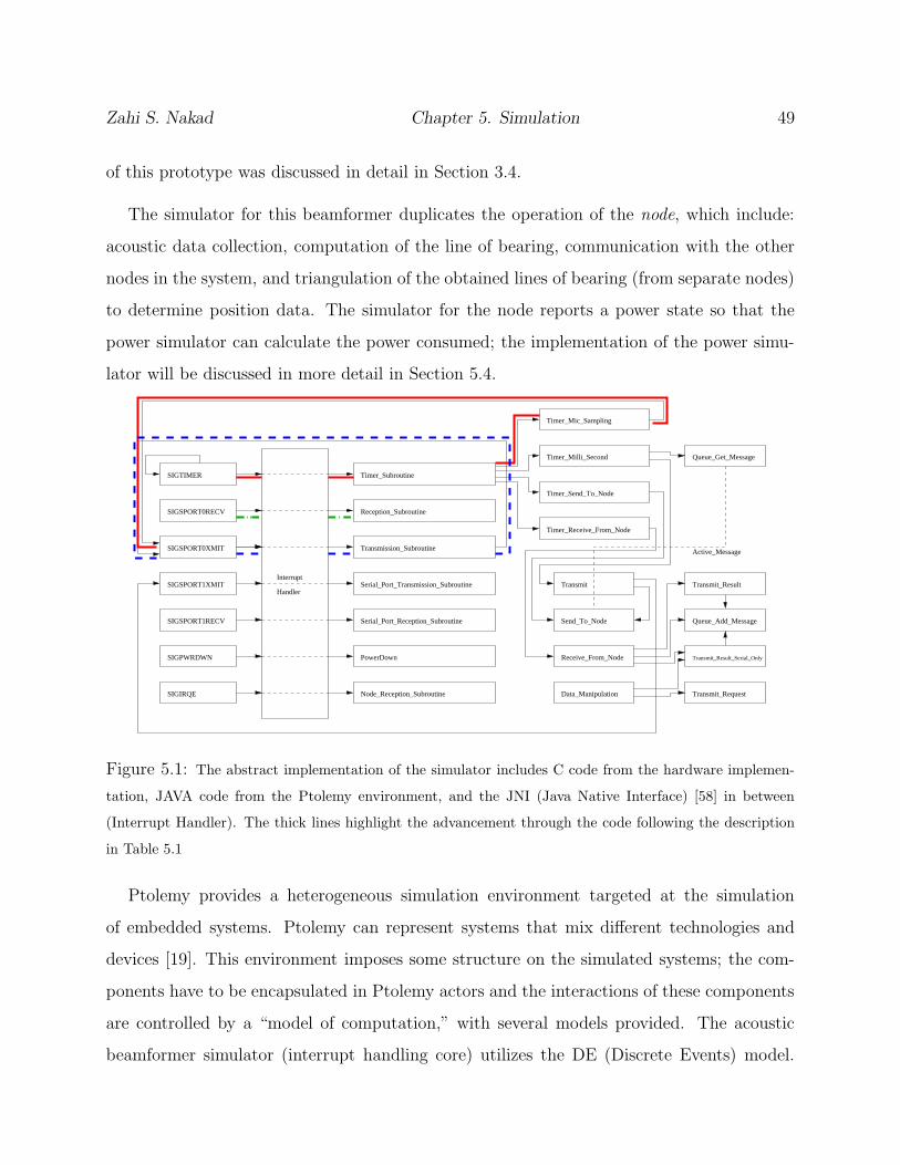
Zahi S. Nakad Chapter 5. Simulation 49
of this prototype was discussed in detail in Section 3.4.
The simulator for this beamformer duplicates the operation of the node, which include:
acoustic data collection, computation of the line of bearing, communication with the other
nodes in the system, and triangulation of the obtained lines of bearing (from separate nodes)
to determine position data. The simulator for the node reports a power state so that the
power simulator can calculate the power consumed; the implementation of the power simu-
lator will be discussed in more detail in Section 5.4.
SIGTIMER
SIGSPORT0RECV
SIGSPORT0XMIT
SIGSPORT1XMIT
SIGSPORT1RECV
SIGPWRDWN
SIGIRQE
Interrupt
Handler
Timer_Subroutine
Transmission_Subroutine
Serial_Port_Transmission_Subroutine
Serial_Port_Reception_Subroutine
PowerDown
Node_Reception_Subroutine
Timer_Mic_Sampling
Timer_Milli_Second
Timer_Send_To_Node
Timer_Receive_From_Node
Reception_Subroutine
Queue_Get_Message
Transmit
Send_To_Node
Receive_From_Node
Transmit_Result
Queue_Add_Message
Transmit_Request
Transmit_Result_Serial_Only
Data_Manipulation
Active_Message
Figure 5.1: The abstract implementation of the simulator includes C code from the hardware implemen-
tation, JAVA code from the Ptolemy environment, and the JNI (Java Native Interface) [58] in between
(Interrupt Handler). The thick lines highlight the advancement through the code following the description
in Table 5.1
Ptolemy provides a heterogeneous simulation environment targeted at the simulation
of embedded systems. Ptolemy can represent systems that mix different technologies and
devices [19]. This environment imposes some structure on the simulated systems; the com-
ponents have to be encapsulated in Ptolemy actors and the interactions of these components
are controlled by a “model of computation,” with several models provided. The acoustic
beamformer simulator (interrupt handling core) utilizes the DE (Discrete Events) model.
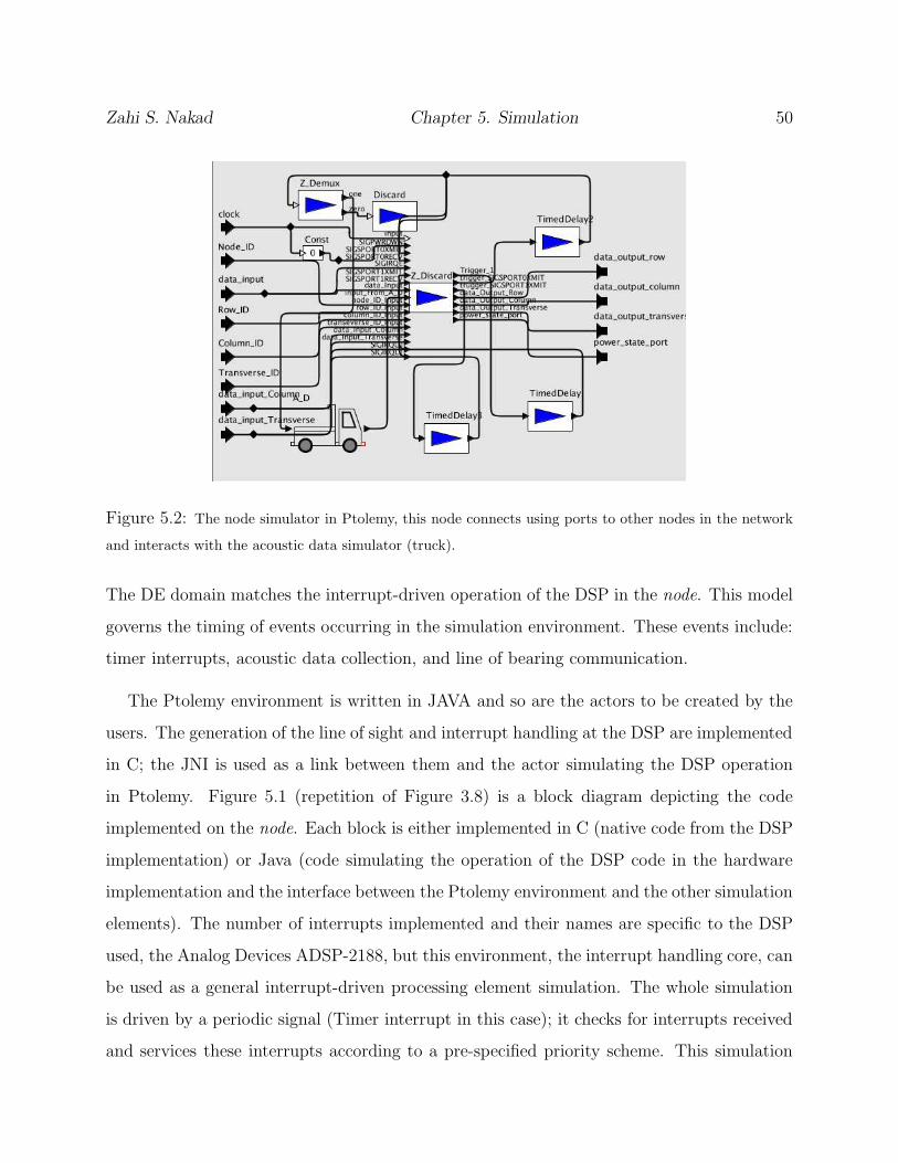
Zahi S. Nakad Chapter 5. Simulation 50
Figure 5.2: The node simulator in Ptolemy, this node connects using ports to other nodes in the network
and interacts with the acoustic data simulator (truck).
The DE domain matches the interrupt-driven operation of the DSP in the node. This model
governs the timing of events occurring in the simulation environment. These events include:
timer interrupts, acoustic data collection, and line of bearing communication.
The Ptolemy environment is written in JAVA and so are the actors to be created by the
users. The generation of the line of sight and interrupt handling at the DSP are implemented
in C; the JNI is used as a link between them and the actor simulating the DSP operation
in Ptolemy. Figure 5.1 (repetition of Figure 3.8) is a block diagram depicting the code
implemented on the node. Each block is either implemented in C (native code from the DSP
implementation) or Java (code simulating the operation of the DSP code in the hardware
implementation and the interface between the Ptolemy environment and the other simulation
elements). The number of interrupts implemented and their names are specific to the DSP
used, the Analog Devices ADSP-2188, but this environment, the interrupt handling core, can
be used as a general interrupt-driven processing element simulation. The whole simulation
is driven by a periodic signal (Timer interrupt in this case); it checks for interrupts received
and services these interrupts according to a pre-specified priority scheme. This simulation

Zahi S. Nakad Chapter 5. Simulation 51
aims at proving functionality and providing a power consumption estimate for the prototype.
The node simultor in Ptolemy is shown in Figure 5.2.
The operation of the simulation will be explained by focusing on a small but representative
part of the code and discussing it in detail. The acoustic data collection shown in Table 5.1
will be used as this representative part because it uses most of the aspects of the simulator
implementation.
5.4 Power Simulation
Rate of power consumption is a crucial measure in stand-alone applications. Simulating
power consumption provides a useful means of varying the operation of an application to
reach a more efficient performance in terms of consumed power. Each processing node can
be operating in one of a set of operation phases. The interrupt handling core reports these
states to the power simulator.
In the Acoustic Beamforming Array, the processing node can be collecting data from the
microphones, performing the beamforming operation, communicating with other nodes in
the fabric, or waiting in the idle state. Physical measurements were performed to collect the
power consumed in these phases. Using these basic values, the parameters of the system can
be changed such as number of microphones and the power consumption values simulated.
Each node in the simulation provides information about its processing states, a power tracker
tracks these changes and based on the measured values computes the power consumption of
the system. Multiple tables in [54] document this simulated data. These tables provide in-
formation about the operation of the prototypes under varying circumstances. The Acoustic
Beamforming Array was the prototype in [54].
This simulation environment was used in [46] to provide energy consumption values while
varying system parameters.The large increase in power consumption values when using wire-
less communication, reported in [46], shows the advantage of using e-textiles in large-area
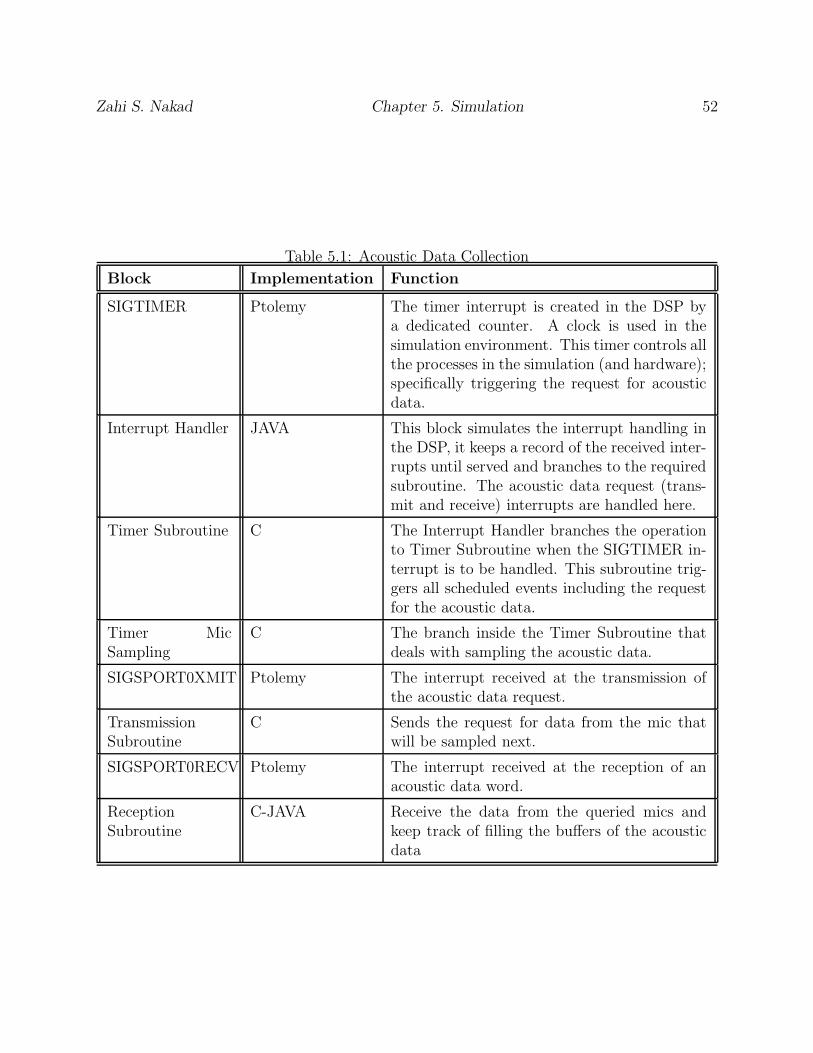
Zahi S. Nakad Chapter 5. Simulation 52
Table 5.1: Acoustic Data Collection
Block Implementation Function
SIGTIMER Ptolemy The timer interrupt is created in the DSP bya dedicated counter. A clock is used in thesimulation environment. This timer controls allthe processes in the simulation (and hardware);specifically triggering the request for acousticdata.
Interrupt Handler JAVA This block simulates the interrupt handling inthe DSP, it keeps a record of the received inter-rupts until served and branches to the requiredsubroutine. The acoustic data request (trans-mit and receive) interrupts are handled here.
Timer Subroutine C The Interrupt Handler branches the operationto Timer Subroutine when the SIGTIMER in-terrupt is to be handled. This subroutine trig-gers all scheduled events including the requestfor the acoustic data.
Timer MicSampling
C The branch inside the Timer Subroutine thatdeals with sampling the acoustic data.
SIGSPORT0XMIT Ptolemy The interrupt received at the transmission ofthe acoustic data request.
TransmissionSubroutine
C Sends the request for data from the mic thatwill be sampled next.
SIGSPORT0RECV Ptolemy The interrupt received at the reception of anacoustic data word.
ReceptionSubroutine
C-JAVA Receive the data from the queried mics andkeep track of filling the buffers of the acousticdata
Zahi S. Nakad Chapter 5. Simulation 53
sensing applications. A study of prolonging the operation of the Acoustic Beamforming
Array by changing the number of power sources and dealing with faults in the power lines
and the processing nodes was presented in [54] using this power simulator. The simula-
tor descibed in Section 5.3 was used in conjuction an actor providing the fault information
(Physical Model) and another actor tracking the power consumption (Power Tracker) to
provide needed simulation [54].
5.5 Communication Simulation
Testing the implemented communication scheme through prototyping will require building
enough hardware prototypes to significantly explore its operation. Simulation of multiple
communicating nodes is more feasible and is viable with the use of the developed simulator.
Figure 5.3 depicts a basic setup of two grids of 16 nodes each connected with a set of trans-
verse links (these links are discussed in detail in Chapter 6). Creating all the connections
by hand for each of the present ports is labor intensive. The representation of the connec-
tions in Ptolemy is done with XML (Extensible Markup Language) [60]. With the use of
XML, large networks and the links between them can be created automatically. Automatic
code generation provides a useful medium for testing different applications and computing
performance metrics, as will be done in Section 6.5.
5.6 Integrating the Fault Simulation and the Commu-
nication Scheme
The communication scheme used in the system will be described in Chapter 6. This scheme
can route around faults and sleeping nodes. The physical world simulator provides support
to test this implementation by attaching a Fabric actor to the actor simulating a node in
the Acoustic Beamforming Array. The Fabric actor shown in Figure 5.4 creates the error

Zahi S. Nakad Chapter 5. Simulation 54
Figure 5.3: Simulation of 32 nodes on two separate grids joined with transverse links.
information that blocks data from crossing the communication channels that exist on the
fabric. This is done by controlling multiplexors through the control signal provided. The
Fabric actor also recognizes that an error in the communication channel can be to the “left”
or the “right” of a node, or on the channel providing the link between the nodes at the ends
of the ring. These channels are depicted in a block diagram in Figure 5.5. When a channel
is disconnected a node detects this error and the fault tolerant process in the networking
scheme deals with the error as discussed in Chapter 6. Figure 5.6 presents the simulator
for the Acoustic Beamforming Array while using these nodes. More communication links
are used in this case to account for the links traversing the ring between the edges. The
physical world simulator was also used in [54] to test for power line disruptions caused by
the introduced faults.
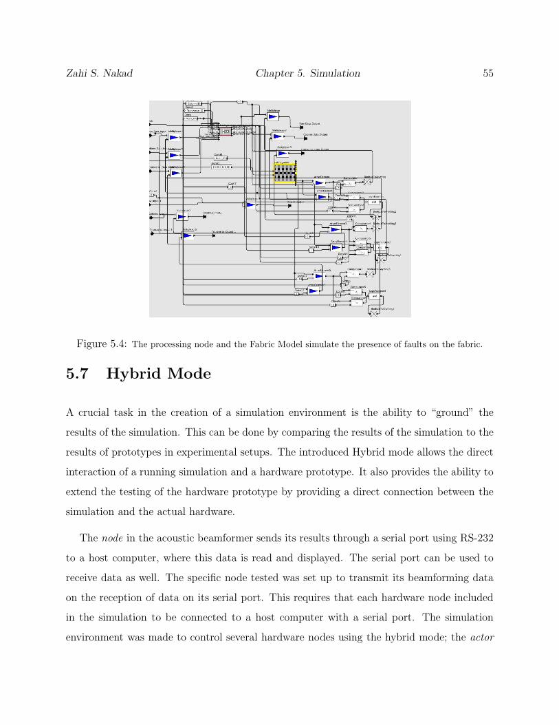
Zahi S. Nakad Chapter 5. Simulation 55
Figure 5.4: The processing node and the Fabric Model simulate the presence of faults on the fabric.
5.7 Hybrid Mode
A crucial task in the creation of a simulation environment is the ability to “ground” the
results of the simulation. This can be done by comparing the results of the simulation to the
results of prototypes in experimental setups. The introduced Hybrid mode allows the direct
interaction of a running simulation and a hardware prototype. It also provides the ability to
extend the testing of the hardware prototype by providing a direct connection between the
simulation and the actual hardware.
The node in the acoustic beamformer sends its results through a serial port using RS-232
to a host computer, where this data is read and displayed. The serial port can be used to
receive data as well. The specific node tested was set up to transmit its beamforming data
on the reception of data on its serial port. This requires that each hardware node included
in the simulation to be connected to a host computer with a serial port. The simulation
environment was made to control several hardware nodes using the hybrid mode; the actor

Zahi S. Nakad Chapter 5. Simulation 56
0
0
0
0
0
0
0
0
0
Processing
Node
Fabric
Model
ROW
ROW
ROW
COLUMN
COLUMN
COLUMN
TRANSVERSETRANSVERSE
TRANSVERSE
Figure 5.5: Multiplexors controlled by signals from the Fabric Model create the errors in the communication
links.
Figure 5.6: Extra connections to the new node, Figure 5.4, are required to represent the connections.
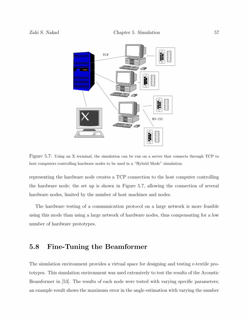
Zahi S. Nakad Chapter 5. Simulation 57
RS−232
TCP
Figure 5.7: Using an X terminal, the simulation can be run on a server that connects through TCP to
host computers controlling hardware nodes to be used in a “Hybrid Mode” simulation.
representing the hardware node creates a TCP connection to the host computer controlling
the hardware node; the set up is shown in Figure 5.7, allowing the connection of several
hardware nodes, limited by the number of host machines and nodes.
The hardware testing of a communication protocol on a large network is more feasible
using this mode than using a large network of hardware nodes, thus compensating for a low
number of hardware prototypes.
5.8 Fine-Tuning the Beamformer
The simulation environment provides a virtual space for designing and testing e-textile pro-
totypes. This simulation environment was used extensively to test the results of the Acoustic
Beamformer in [53]. The results of each node were tested with varying specific parameters;
an example result shows the maximum error in the angle estimation with varying the number

Zahi S. Nakad Chapter 5. Simulation 58
Processing Node
Sensing Element
Node to Node Link
Sensor to Node Link
Figure 5.8: A general concept of an e-textile including the nodes, sensors, and communication channels.
of microphones used and the sampling rate (radius of cluster was fixed to 3 feet, and the SNR
(Signal to Noise Ratio) to 5dB). The simulator was also used to test the operation of the
Acoustic Beamforming Array in providing the location of the vehicle while using different
numbers of clusters at specific distances.
The simulator helped us in fine-tuning the acoustic beamformer, by changing specific
variables and recording the changes in accuracies and power consumption, before deciding
on a major change in the implementation. A general concept of e-textile systems based on
the acoustic array is shown in Fig. 5.8. This concept will help us in specifying the variables
that would be changed in a simulation environment. The significant variables that affect
the operation and power consumption of such a system are the number of clusters in the
system, the number of sensors associated with each node, the format of the data transmitted
between sensor and node (analog or digital), sampling rate, communication bandwidth and
size of data chunks (sensor-node and node-node communication), to name a few [59].

Chapter 6
Networking
A networking scheme designed for e-textile applications will be discussed in this chapter.
The scheme is based on the Token Grid described in Section 2.1.2. The modifications to this
network are based upon the precepts stated in the electronic textile architecture detailed in
Chapter 4.
The number of hops a token has to traverse is directly related to the number of nodes
on the ring. In the case of large area e-textiles, a large number of nodes in a ring can slow
the communication on the ring. Fabric swatches will be connected to form large or wearable
fabrics (precept of the electronic textile architecture); the networks on these different fabrics
must be connected. The addition of a third dimension to the networking scheme to address
both of these issues will be discussed in Section 6.1.
Fault tolerance was integrated in the design of the networking scheme in accordance with
the fault-tolerant communication scheme precept. The new fault-tolerance scheme differs
from the Token Grid scheme for two main reasons. First, the Token Grid scheme assumes
no faults on the communication links. Second, the Token Grid scheme assumes that the
processing nodes will have the ability to forward data in the case of a failure. Both of these
assumptions do not apply to e-textiles and thus a new scheme, presented in Section 6.2,
59
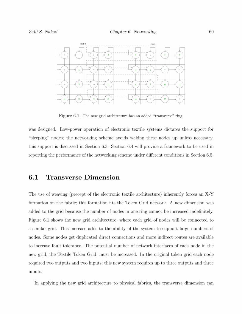
Zahi S. Nakad Chapter 6. Networking 60
0 1 2 3
5 6 7
10 11
13 14 15
8
4
9
12
0 1 2 3
5 6 7
10 11
13 14 15
8
4
9
12
GRID 0 GRID 1
Figure 6.1: The new grid architecture has an added “transverse” ring.
was designed. Low-power operation of electronic textile systems dictates the support for
“sleeping” nodes; the networking scheme avoids waking these nodes up unless necessary,
this support is discussed in Section 6.3. Section 6.4 will provide a framework to be used in
reporting the performance of the networking scheme under different conditions in Section 6.5.
6.1 Transverse Dimension
The use of weaving (precept of the electronic textile architecture) inherently forces an X-Y
formation on the fabric; this formation fits the Token Grid network. A new dimension was
added to the grid because the number of nodes in one ring cannot be increased indefinitely.
Figure 6.1 shows the new grid architecture, where each grid of nodes will be connected to
a similar grid. This increase adds to the ability of the system to support large numbers of
nodes. Some nodes get duplicated direct connections and more indirect routes are available
to increase fault tolerance. The potential number of network interfaces of each node in the
new grid, the Textile Token Grid, must be increased. In the original token grid each node
required two outputs and two inputs; this new system requires up to three outputs and three
inputs.
In applying the new grid architecture to physical fabrics, the transverse dimension can
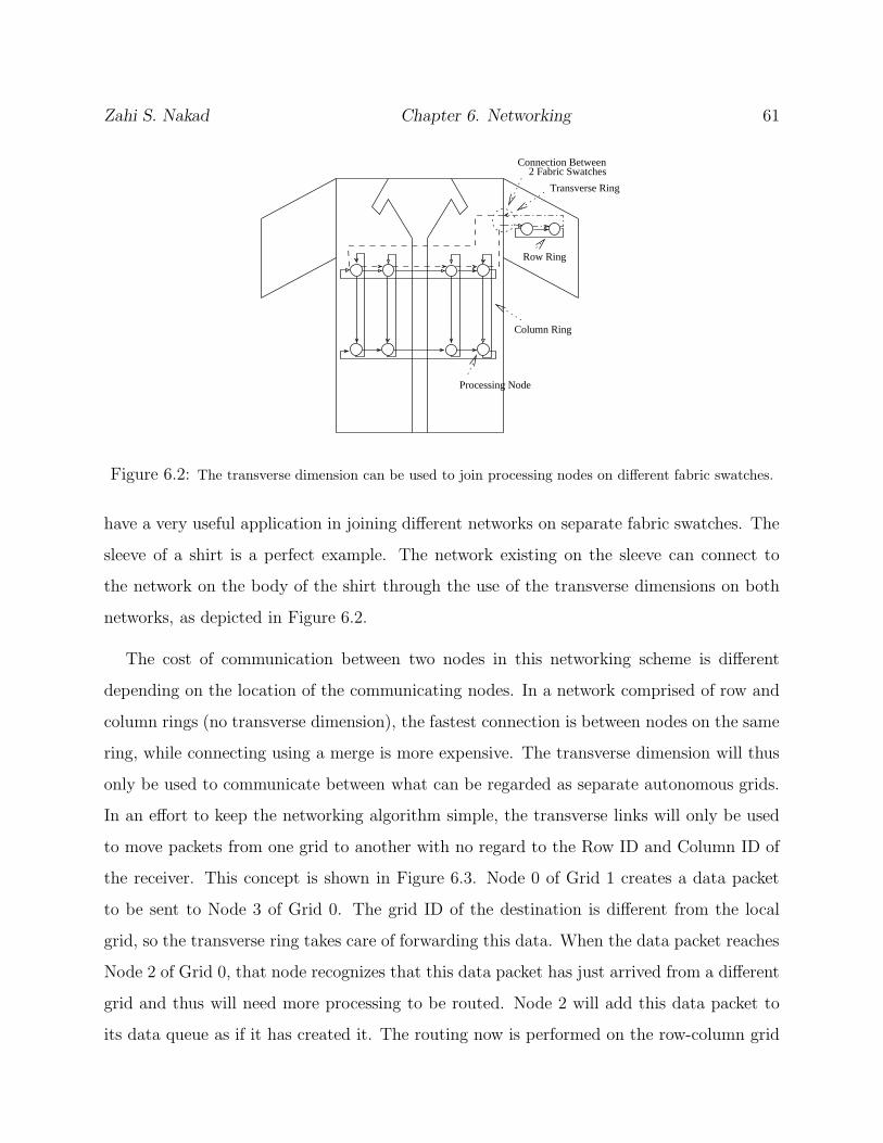
Zahi S. Nakad Chapter 6. Networking 61
Transverse Ring
Processing Node
Row Ring
Column Ring
Connection Between2 Fabric Swatches
Figure 6.2: The transverse dimension can be used to join processing nodes on different fabric swatches.
have a very useful application in joining different networks on separate fabric swatches. The
sleeve of a shirt is a perfect example. The network existing on the sleeve can connect to
the network on the body of the shirt through the use of the transverse dimensions on both
networks, as depicted in Figure 6.2.
The cost of communication between two nodes in this networking scheme is different
depending on the location of the communicating nodes. In a network comprised of row and
column rings (no transverse dimension), the fastest connection is between nodes on the same
ring, while connecting using a merge is more expensive. The transverse dimension will thus
only be used to communicate between what can be regarded as separate autonomous grids.
In an effort to keep the networking algorithm simple, the transverse links will only be used
to move packets from one grid to another with no regard to the Row ID and Column ID of
the receiver. This concept is shown in Figure 6.3. Node 0 of Grid 1 creates a data packet
to be sent to Node 3 of Grid 0. The grid ID of the destination is different from the local
grid, so the transverse ring takes care of forwarding this data. When the data packet reaches
Node 2 of Grid 0, that node recognizes that this data packet has just arrived from a different
grid and thus will need more processing to be routed. Node 2 will add this data packet to
its data queue as if it has created it. The routing now is performed on the row-column grid
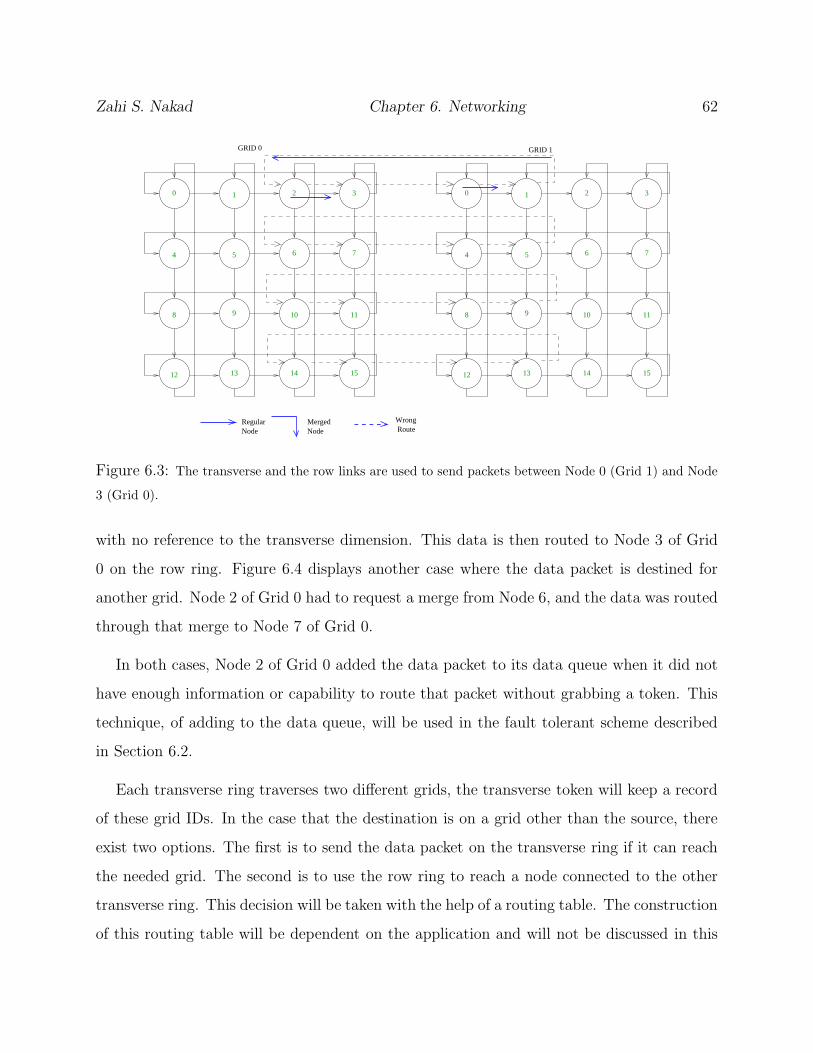
Zahi S. Nakad Chapter 6. Networking 62
0 1 2 3
5 6 7
10 11
13 14 15
8
4
9
12
RegularNode
Merged Node Route
Wrong
0 1 2 3
5 6 7
10 11
13 14 15
8
4
9
12
GRID 0 GRID 1
Figure 6.3: The transverse and the row links are used to send packets between Node 0 (Grid 1) and Node
3 (Grid 0).
with no reference to the transverse dimension. This data is then routed to Node 3 of Grid
0 on the row ring. Figure 6.4 displays another case where the data packet is destined for
another grid. Node 2 of Grid 0 had to request a merge from Node 6, and the data was routed
through that merge to Node 7 of Grid 0.
In both cases, Node 2 of Grid 0 added the data packet to its data queue when it did not
have enough information or capability to route that packet without grabbing a token. This
technique, of adding to the data queue, will be used in the fault tolerant scheme described
in Section 6.2.
Each transverse ring traverses two different grids, the transverse token will keep a record
of these grid IDs. In the case that the destination is on a grid other than the source, there
exist two options. The first is to send the data packet on the transverse ring if it can reach
the needed grid. The second is to use the row ring to reach a node connected to the other
transverse ring. This decision will be taken with the help of a routing table. The construction
of this routing table will be dependent on the application and will not be discussed in this

Zahi S. Nakad Chapter 6. Networking 63
0 1 2 3
5 6 7
10 11
13 14 15
8
4
9
12
RegularNode
Merged Node Route
Wrong
0 1 2 3
5 6 7
10 11
13 14 15
8
4
9
12
GRID 0 GRID 1
Figure 6.4: The data packet is treated as a new packet inside the receiving grid. Node 0 Grid 1 uses the
transverse ring to reach Node 2 Grid 0, at Node 2 the packet is re-processed for routing and it is sent through
a merge to Node 7 Grid 0.
dissertation. Figure 6.5 depicts a case where the row ring is needed before the data packet
can reach the destination grid.
6.1.1 Size of the Grid
The size of the grid dictates the number of nodes in the rings. This is a decision metric that
can affect the operation of the network. The values in Table 6.2 and Table 6.3, Section 6.4,
show that communication inside the same ring is the fastest. The number of nodes in a ring
directly affects TWtoken (time to wait for a token) and thus controls the total waiting time
and the number of hops each communication has to experience. The number of nodes in each
ring also dictates the number of grids. Communication on transverse links (between grids)
is more expensive and thus should be minimized. The boundaries between grids should be
chosen considering the communication needs of the application.
In the presence of faults, a tear across the width of a fabric will totally sever the connection

Zahi S. Nakad Chapter 6. Networking 64
0 1 2 3
5 6 7
10 11
13 14 15
8
4
9
12
RegularNode
Merged Node Route
Wrong
0 1 2 3
5 6 7
10 11
13 14 15
8
4
9
12
GRID 0 GRID 1
Figure 6.5: Node 2 of Grid 1 uses its row ring to forward the data packet to another transverse ring to
reach Grid 0.
between the two parts, thus creating an almost useless grid. The larger the number of nodes
in this grid the more significant the loss of nodes in the overall prototype. As a qualitative
view, the number of nodes in a ring should be small enough to keep the communication
speed-up and reduce the losses when a large tear occurs. The increase in communication
cost across transverse links requires the use of enough nodes inside rings to span enough
area to minimize the need for transverse connections. These views provide guidelines into
deciding the sizes of separate grids. In wearable systems, the flexibility of choosing the grid
size is constrained by the fabric swatches determined by the design of the garment.
6.2 Fault Tolerant Implementation
The implementation of a fault tolerant communication scheme is a must for electronic textiles
systems. The following section discusses the fault tolerant scheme used in this architecture.
Detection of errors and propagating information about the faults are the first aspects pre-

Zahi S. Nakad Chapter 6. Networking 65
0 1 2 3
Figure 6.6: Node 1 has an error at the link directly to its “left.”
sented. Utilization of this information in routing data is then discussed.
6.2.1 Creation of Error packets
The implemented fault tolerant scheme, discussed in detail in Section 6.2.2, requires that the
nodes in the system update error information about the network. The detection of errors
and the transmission of this information will be detailed in this section.
Error detection
Each node is connected to three different rings (row, column, and transverse). There are
three possibilities for link errors. In the case that there are no data packets to be sent on any
link, the nodes will forward the tokens. Each node will keep three separate Timeout Counters
pertaining to each link it is connected to. These counters are reset to zero at the reception
of any data (tokens, data packets, and error packets). If any of these counters reaches a
pre-specified value an error is declared. This value will be dependent on the application and
the specific topology; in this research it is set empirically. When an error is detected in this
manner it means that there is an error to the “left” of the node. Figure 6.6 shows a specific
example, Node 1 does not receive anything from its ring and after the timeout period it
creates an error packet and sends it down the ring. Node 1 will also update a flag that states
that the row it belongs to is in error. When a node receives an error packet it forwards that
packet down the same ring and updates the flag stating that the ring is in error.
A situation may arise where Node 2 will reach its timeout value before it receives the error
packet from Node 1. To determine which node is actually on the broken link, a temporary

Zahi S. Nakad Chapter 6. Networking 66
0 1 2 3
Figure 6.7: Node 1 and Node 3 have errors at the links directly to their “left.”
error flag is used. When a node first reaches its timeout counter it sends the error packet
and sets the temporary error flag. The error flag is not set unless the timeout period is
reached while the temporary error flag is asserted. Following Figure 6.6, Node 2 will receive
an error packet from Node 1 after it sends its own. This reception will reset the temporary
error flag and thus Node 2 knows that there is an error on the ring and that error is on the
link directly to the left of Node 1, the source of the error packet. Figure 6.7 depicts a case
where there are two different errors on the same ring. The nodes on the ring will all have
the information that there is an error on the ring. Following the scheme mentioned above
Node 0 will have the information that Node 3 has an immediate error and Node 2 will have
the same information about Node 1.
Error information propagation
Using the process discussed above, each node on a ring with an error has a flag that reflects
that information. This information is to be propagated to other nodes in the network. If the
error is on the row ring, then the column token that passes through each of these nodes will
be updated to reflect that the specific row ring has an error. This has no propagation costs
because the token is already traversing the whole column ring. Each node will have to keep
another variable that pertains to errors. This variable will carry the information of errors on
other rings in the network; three variables will be needed reflecting the information about
the other rows, columns, and transverses in the network.
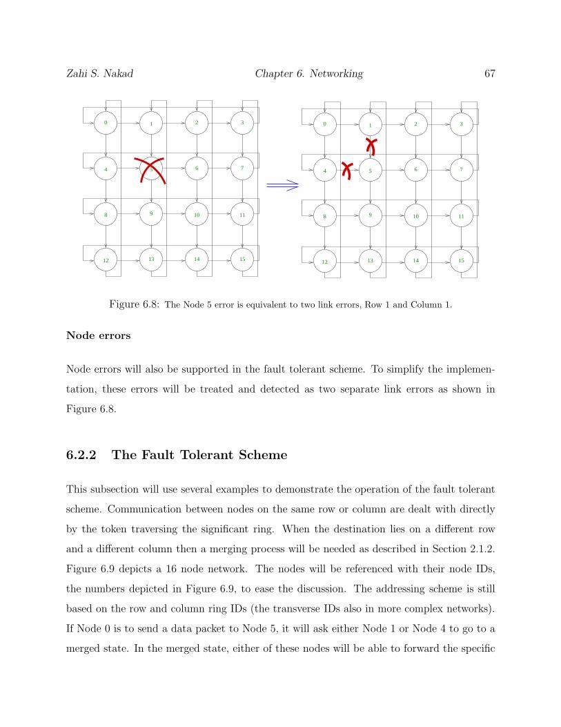
Zahi S. Nakad Chapter 6. Networking 67
0 1 2 3
5 6 7
10 11
13 14 15
8
4
9
12
0 1 2 3
5 6 7
10 11
13 14 15
8
4
9
12
Figure 6.8: The Node 5 error is equivalent to two link errors, Row 1 and Column 1.
Node errors
Node errors will also be supported in the fault tolerant scheme. To simplify the implemen-
tation, these errors will be treated and detected as two separate link errors as shown in
Figure 6.8.
6.2.2 The Fault Tolerant Scheme
This subsection will use several examples to demonstrate the operation of the fault tolerant
scheme. Communication between nodes on the same row or column are dealt with directly
by the token traversing the significant ring. When the destination lies on a different row
and a different column then a merging process will be needed as described in Section 2.1.2.
Figure 6.9 depicts a 16 node network. The nodes will be referenced with their node IDs,
the numbers depicted in Figure 6.9, to ease the discussion. The addressing scheme is still
based on the row and column ring IDs (the transverse IDs also in more complex networks).
If Node 0 is to send a data packet to Node 5, it will ask either Node 1 or Node 4 to go to a
merged state. In the merged state, either of these nodes will be able to forward the specific
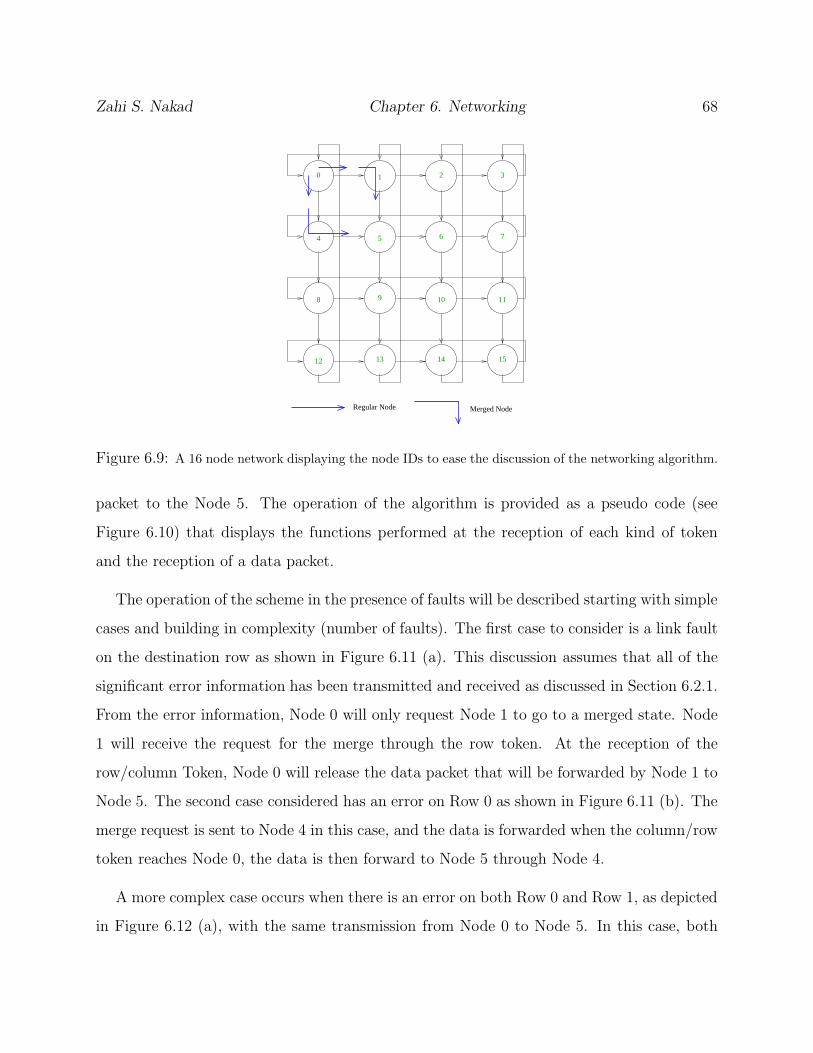
Zahi S. Nakad Chapter 6. Networking 68
0 1 2 3
5 6 7
10 11
13 14 15
8
4
9
12
Regular Node Merged Node
Figure 6.9: A 16 node network displaying the node IDs to ease the discussion of the networking algorithm.
packet to the Node 5. The operation of the algorithm is provided as a pseudo code (see
Figure 6.10) that displays the functions performed at the reception of each kind of token
and the reception of a data packet.
The operation of the scheme in the presence of faults will be described starting with simple
cases and building in complexity (number of faults). The first case to consider is a link fault
on the destination row as shown in Figure 6.11 (a). This discussion assumes that all of the
significant error information has been transmitted and received as discussed in Section 6.2.1.
From the error information, Node 0 will only request Node 1 to go to a merged state. Node
1 will receive the request for the merge through the row token. At the reception of the
row/column Token, Node 0 will release the data packet that will be forwarded by Node 1 to
Node 5. The second case considered has an error on Row 0 as shown in Figure 6.11 (b). The
merge request is sent to Node 4 in this case, and the data is forwarded when the column/row
token reaches Node 0, the data is then forward to Node 5 through Node 4.
A more complex case occurs when there is an error on both Row 0 and Row 1, as depicted
in Figure 6.12 (a), with the same transmission from Node 0 to Node 5. In this case, both

Zahi S. Nakad Chapter 6. Networking 69
- Row Token Arrival:
- if(Data Packet ready for sending):
- If(Destination on same Grid):
- If(Destination on same row): Send data directlyon Row ring.
- else:
- If(Destination on same Column):Column Token will take care of it, no action.
- else: Need a Merger, request onefrom node on the same row as this, and samecolumn as destination. This information is addedto the token that is later released.
- else: Transverse Token will take care of it, no action.
- else: No Action
- If(Waiting For Row Token == 1):
- //Column Token has been captured
- Create a Row Column Token
- Merged Status = 1;
- Waiting For Row Token = 0;
- Send Token on Row ring.
- If(Merged Status == 0):
- If this node was asked to go to a merged state:
- Grab the token
- Waiting For Column Token = 1;
- else: Release the Row Token on the Row ring.
(a)
- Column Token Arrival:
- if(Data Packet ready for sending):
- If(Destination on same Grid):
- If(Destination on same column:) Send data directlyon Column ring.
- else:
- If(Destination on same Row):Row Token will take care of it, no action.
- else: Need a Merger, request onefrom node on the same column as this, and same rowas destination. This information is added to thetoken that is later released.
- else: Transverse Token will take care of it, no action.
- else: No Action
- If(Waiting For Column Token == 1):
- //Row Token has been captured
- Create a Row Column Token
- Merged Status = 1;
- Waiting For Column Token = 0;
- Send Token on Row ring.
- If(Merged Status == 0):
- If this node was asked to go to a merged state:
- Grab the token
- Waiting For Row Token = 1;
- else: Release the Column Token on the Column ring.
(b)
- Row Column Token Arrival:
- if(Data Packet ready for sending):
- If(Destination on same Grid):
- if(Destination Column == Column of Master of Token)&& (This node on a different Row than Destination)
- if this is the master node:
Send data on Column ring.
- else: Send data on Row ring.
- else: Transverse Token will take care of it, no action.
- else: No Action
- if(This is the node that created the Row Column Token)
- Create Column Row Token
- Send Token on Column ring.
- else: Release the Row Column on Row ring.
(c)
- Column Row Token Arrival:
- if(Data Packet ready for sending):
If(Destination on same Grid):
- if(Destination Row == Row of Master of Token)&& (This node on a different Column than Destination)
- if this is the master node:Send data on Row ring.
- else: Send data on Column ring.
else: Transverse Token will take care of it, no action.
- else: No Action
- if(This is the node that created the Column Row Token)
- //The Merged tokens have finished traversing the merged ring.
- Create Row Token and send it on Row ring.
- Create Column Token and send it on Column ring.
- else: Release the Column Row on Column ring.
(d)
- Data Packet Arrival:
- if(Data Packet is meant for this node): DONE
- else:
- if(Destination on same Grid):
- switch(Channel data recieved on)
- case(Row): if(Merged Status == 0): Forward on Row. Else: Forward on Column.
- case(Column): if(Merged Status == 0): Forward Column. Else: Forward Row.
- case(Transverse): Data just arrived from another grid, add it to then Data Queueto be processed later for forwarding.
- else:
- if Data received on Transverse ring: Forward Data on Transverse
- else: Let the Transverse Token deal with forwarding this packet.
(e)
Figure 6.10: The operation of the algorithm is controlled by these separate processes.
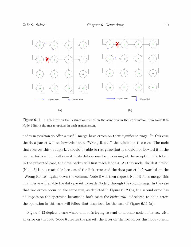
Zahi S. Nakad Chapter 6. Networking 70
0 1 2 3
5 6 7
10 11
13 14 15
8
4
9
12
Regular Node Merged Node
(a)
0 1 2 3
5 6 7
10 11
13 14 15
8
4
9
12
Regular Node Merged Node
(b)
Figure 6.11: A link error on the destination row or on the same row in the transmission from Node 0 to
Node 5 limits the merge options in each transmission.
nodes in position to offer a useful merge have errors on their significant rings. In this case
the data packet will be forwarded on a “Wrong Route,” the column in this case. The node
that receives this data packet should be able to recognize that it should not forward it in the
regular fashion, but will save it in its data queue for processing at the reception of a token.
In the presented case, the data packet will first reach Node 4. At that node, the destination
(Node 5) is not reachable because of the link error and the data packet is forwarded on the
“Wrong Route” again, down the column. Node 8 will then request Node 9 for a merge; this
final merge will enable the data packet to reach Node 5 through the column ring. In the case
that two errors occur on the same row, as depicted in Figure 6.12 (b), the second error has
no impact on the operation because in both cases the entire row is declared to be in error;
the operation in this case will follow that described for the case of Figure 6.11 (a).
Figure 6.13 depicts a case where a node is trying to send to another node on its row with
an error on the row. Node 6 creates the packet, the error on the row forces this node to send

Zahi S. Nakad Chapter 6. Networking 71
0 1 2 3
5 6 7
10 11
13 14 15
8
4
9
12
RegularNode
Merged Node Route
Wrong
(a)
0 1 2 3
5 6 7
10 11
13 14 15
8
4
9
12
Regular Node Merged Node
(b)
Figure 6.12: Link errors on Row 0 and Row 1 prevent a regular merging scheme and force a “Wrong
Route.” Two link errors on Row 1 affect the operation in the same manner as a single error.
the packet on a “Wrong Route” down the column to Node 10. Node 10 requests Node 9 to
merge. When the merging process is finished the data packet will be routed from Node 10
through Row 2 to Node 9 that routes the packet through Column 1 to Node 5.
Figure 6.14 presents the pseudo code that responds to a data packet reception. The
pseudo code is presented in two forms: the first assumes no faults in the network, the second
utilizes the received error information to correctly route the data packet or push it on its data
queue for later processing at the reception of a token. The operation of the fault tolerant
pseudo code follows closely the simpler version, but it detects the case of a “Wrong Route”
and uses the same method of re-processing this data as when a data packet is received from
another grid. The fault tolerant pseudo codes for the other events are more complex and are
provided in Appendix A.

Zahi S. Nakad Chapter 6. Networking 72
0 1 2 3
5 6 7
10 11
13 14 15
8
4
9
12
RegularNode
Merged Node Route
Wrong
Figure 6.13: The path of a data packet from Node 6 to Node 5 with an error on Row 1.
6.2.3 The Fault Tolerant Scheme on the Transverse Link
The transverse links in the network carry packets destined to a grid different from their
source. The forwarding of these packets on the transverse links is done in a manner unrelated
to their specific destination. Any node that receives a packet on its transverse link whose
destination is on the same grid adds this packet to its data queue and processes it later
for forwarding on the grid. This simplistic approach to grid-to-grid forwarding supports a
simple fault-tolerant scheme on the transverse links. When a node needs to forward a packet
on its transverse link and there is an error on that link, a “Wrong Route” is forced down
the column. This also applies when the data is destined for another grid but is forwarded
on the row ring to reach the appropriate transverse ring. These two cases are depicted in
Figure 6.15 and Figure 6.16. In Figure 6.15 Node 0 uses the “Wrong Route” to reach Node
3, and Node 3 then uses its transverse ring to forward the packet to Grid 0. In Figure 6.16,
Node 2 must forward the packet on its row ring to reach the correct transverse ring. The
row error forced Node 2 to use the “Wrong Route” to reach Node 6. Node 6 uses its row
ring to forward the packet to the correct transverse ring and from there to Grid 0.

Zahi S. Nakad Chapter 6. Networking 73
- Data Packet Arrival:
- if(Data Packet is meant for this node): DONE
- else:
- if(Destination on same Grid):
- switch(Channel data recieved on)
- case(Row): if(Merged Status == 0): Forward on Row. Else: Forward on Column.
- case(Column): if(Merged Status == 0): Forward Column. Else: Forward Row.
- case(Transverse): Data just arrived from another grid, add it to then Data Queueto be processed later for forwarding.
- else:
- if Data received on Transverse ring: Forward Data on Transverse
- else: Let the Transverse Token deal with forwarding this packet.
(a)
- Data Packet Arrival:
- if(This is the source of the Data Packet): DISCARD
- if(Data Packet is meant for this node): DONE
- else:
- if(Destination on same Grid):
- switch(Channel data recieved on)
- case(Row):
- if((Destination Row != Row ID)&&(Destination Column != Column ID)):can be a “Wrong Route” or Merged Ring
- if(there is a column error on column before): re-process the packet.
- else:
- if(Merged Status == 0): Forward on Row ring.
- else: Forward on Column ring.
- case(Column):
- if((Destination Row != Row ID)&&(Destination Column != Column ID)):can be a “Wrong Route” or Merged Ring
- if(there is a row error on row before): re-process the packet.
- else:
- if(Merged Status == 0): Forward on Column ring.
- else: Forward on Row ring.
- case(Transverse):
- Data just arrived from another grid, add it to the Data Queue to be processed later
for forwarding.
- else:
- if Data received on Transverse ring: Forward Data on Transverse
- else: Let the Transverse Token deal with forwarding this packet.
(b)
Figure 6.14: The Data Packet Arrival pseudo codes with and without fault tolerance implemented.
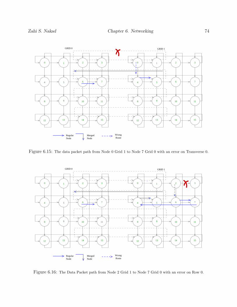
Zahi S. Nakad Chapter 6. Networking 74
RegularNode
Merged Node Route
Wrong
0 1 2 3
5 6 7
10 11
13 14 15
8
4
9
12
GRID 0 GRID 1
0 1 2 3
5 6 7
10 11
13 14 15
8
4
9
12
Figure 6.15: The data packet path from Node 0 Grid 1 to Node 7 Grid 0 with an error on Transverse 0.
RegularNode
Merged Node Route
Wrong
0 1 2 3
5 6 7
10 11
13 14 15
8
4
9
12
GRID 0 GRID 1
0 1 2 3
5 6 7
10 11
13 14 15
8
4
9
12
Figure 6.16: The Data Packet path from Node 2 Grid 1 to Node 7 Grid 0 with an error on Row 0.

Zahi S. Nakad Chapter 6. Networking 75
6.3 Sleeping Nodes
The network has to operate in the presence of faults and sleeping nodes. When a node enters
a sleeping mode it creates the same effect a node failure has on the network as shown in
Figure 6.8. The network has to support sleeping nodes in the same manner a failure is dealt
with; the only difference is that a sleeping node can be re-activated. The network also avoids
waking sleeping nodes unless necessary.
Before a node enters a sleep mode, it sends a sleep packet on its rings in the same manner
an error packet was sent. The information is propagated through the network in the same
manner as the error information. There are two ways a node can be re-activated: the first
is through its own hardware, and the second is through reception from another node in the
network.
In the Acoustic Beamforming Array when a node receives a strong audio signal it is re-
activated. When a node is re-activated it declares itself master of the rings it is connected
to. These rings are not functional since the tokens are not circulating. The nodes that
receive the new tokens update their information pertaining to the sleeping node and this
same information is propagated through the network.
A sleeping node can be awakened by another node in the network. If a node needs to
communicate with a sleeping node (the row and column of the destination node are asleep)
it creates a special data packet and sends it on its row and column. In regular operation of
forwarding data packets, a packet is discarded if its destination row and column are in error.
In this case that packet will be forwarded based on the following scheme. If this packet is
received on the row and the node belongs to the row of the source, then it forwards the
wake-up packet on the row and column. If the data is received on the row and the node
belongs to the source column, then discard the packet. If the node does not belong to any
source rings, then forward on the row. The same process is repeated when receiving from the
column. If the source receives a wake-up packet, it is discarded. The following is a pseudo
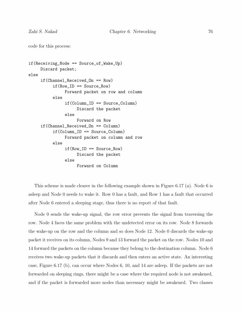
Zahi S. Nakad Chapter 6. Networking 76
code for this process:
if(Receiving_Node == Source_of_Wake_Up)
Discard packet;
else
if(Channel_Received_On == Row)
if(Row_ID == Source_Row)
Forward packet on row and column
else
if(Column_ID == Source_Column)
Discard the packet
else
Forward on Row
if(Channel_Received_On == Column)
if(Column_ID == Source_Column)
Forward packet on column and row
else
if(Row_ID == Source_Row)
Discard the packet
else
Forward on Column
This scheme is made clearer in the following example shown in Figure 6.17 (a). Node 6 is
asleep and Node 0 needs to wake it. Row 0 has a fault, and Row 1 has a fault that occurred
after Node 6 entered a sleeping stage, thus there is no report of that fault.
Node 0 sends the wake-up signal, the row error prevents the signal from traversing the
row. Node 4 faces the same problem with the undetected error on its row. Node 8 forwards
the wake-up on the row and the column and so does Node 12. Node 0 discards the wake-up
packet it receives on its column, Nodes 9 and 13 forward the packet on the row. Nodes 10 and
14 forward the packets on the column because they belong to the destination column. Node 6
receives two wake-up packets that it discards and then enters an active state. An interesting
case, Figure 6.17 (b), can occur where Nodes 6, 10, and 14 are asleep. If the packets are not
forwarded on sleeping rings, there might be a case where the required node is not awakened,
and if the packet is forwarded more nodes than necessary might be awakened. Two classes

Zahi S. Nakad Chapter 6. Networking 77
0 1 2 3
5 6 7
10 11
13 14 15
8
4
9
12
RegularNode
Merged Node
(a)
0 1 2 3
5 6 7
10 11
13 14 15
8
4
9
12
RegularNode
Merged Node
(b)
Figure 6.17: Forwarding the wake-up packet depends on the type of the wake-up required. The lack of
links denotes the rings affected by the sleeping nodes.
of wake-up signals are created to solve this problem. If a node is not awake after the first
trial, another class of wake-up signal is used.
6.4 Enumeration of Transmission Costs
An enumeration of the cost to send a packet from a source to a destination is needed to
provide any study on the performance of the network under varying fault schemes. Given
the networking scheme used, the location of the destination has a direct effect on the amount
of processing and forwarding required from the network and the nodes in question. The
following section will study the different costs attributed to sending a data packet from a
fixed node to a set of different destinations. Two costs will be presented, the first represents
the cost of transmission for the source node, the second represents the number of hops in

Zahi S. Nakad Chapter 6. Networking 78
the network to reach the destination.
The simplest case is sending to a node on the same ring (a ring can be a row, column, or
transverse). The first step is to wait for the token TWtoken. After the token is captured, the
node can send the data packet. The time needed to send this packet is TSdata. After that
the node can release the token. The operation of the network requires that a token is always
rotated around the ring; thus, the extra cost of sending the data packet is the parameter,
TSdata. Table 6.1 presents a set of variables that will be used throughout this in reporting
measures of network performance.
To clarify the presented values in Table 6.1, a more in-depth discussion of some terms
is presented. TWtoken is the waiting time experienced by a node that needs to send a
data packet. The first assumption is that the token is not held in the current node and
that it has been released to the ring earlier. This assumption simplifies the discussion by
not considering cases where the node is actively releasing the token to the ring, thus the
time needed to finish sending the remaining part of the token will have to be considered in
TWtoken. Another simplifying assumption is that the processing time inside a node and the
link latencies are negligible. Using these two assumptions, TWtoken becomes the number of
hops the token needs to reach the sending node multiplied by the time needed to send the
token (TStoken). If node 0 in Figure 6.18 is the sending node, then TWtoken has a minimum
value of TStoken when the token is in Node 3 and a maximum value of (N - 1)TStoken =
3(TStoken) when the token is in Node 1. There are three different cases for this ring with
wait values of 1, 2, or 3 multiples of TStoken; the average is then 2(TStoken) = (N/2)(TStoken).
TS ttokenCost: 3( ) TS ttoken )Cost: (
0 1 2 3
Sending Node
Figure 6.18: The time to wait for the token depends on the location of the token in the ring. The average
case is (N/2)(TStoken).
The operation of the networking scheme is that it sends a row/column token when a node

Zahi S. Nakad Chapter 6. Networking 79
Table 6.1: Nomenclatures and Variables used in the discussion.
Variable Name Value Explanation
Grid - A set of connected Rows and Columns
Ring - Row, Column, or Transverse
N - Number of nodes in a ring.
N2 - Number of nodes in a Grid (NRow = NColumn).
BW - Bandwidth of the communication links.
TStoken Sizetoken/BW Time required to transmit a token.
TWtoken min1 TStoken Time required to wait for reception of token
max2 (N - 1)TStoken (min) Preceding node is sending the token
average (N/2)TStoken (max) Following node is sending the token
TSdata Sizedata/BW Time required to transmit a data packet
TWrc−token min3 TStoken Time required to wait for reception of token
max (N - 1)TStoken (min) Preceding node is sending the token
average (N/2)TStoken (max) Farthest node is sending the token
TWcr−token TWrc−token
TWmerged−token TWtoken+ Token carrying request to reach merging node
(sending with TWtoken+ Time required to capture the other token
row column) TWrc−token+ Time required to wait for row column token.
TWmerged−token TWtoken+ Token carrying request to reach merging node
(sending with TWtoken+ Time required to capture the other token
column row) TWrc−token+ Time required to wait for row column token.
TWcr−token Time required to wait for column row token.
TWmerged−token 2(TWtoken) + Assuming equal distribution between
(average) 1.5(TWtoken) rc and cr merged tokens1The Node processing times and the link latencies are considered negligible to simplify the discussion.
2Considering there are no other data packet transmissions (light load).3rc-token : row column token, cr-token: column row token.
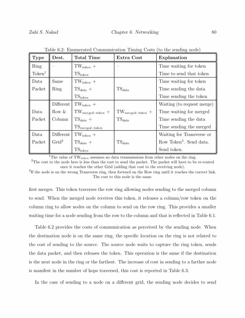
Zahi S. Nakad Chapter 6. Networking 80
Table 6.2: Enumerated Communication Timing Costs (to the sending node)
Type Dest. Total Time Extra Cost Explanation
Ring – TWtoken + – Time waiting for token
Token1 TStoken Time to send that token
Data Same TWtoken + Time waiting for token
Packet Ring TSdata + TSdata Time sending the data
TStoken Time sending the token
Different TWtoken + Waiting (to request merge)
Data Row & TWmerged−token + TWmerged−token + Time waiting for merged
Packet Column TSdata + TSdata Time sending the data
TSmerged−token Time sending the merged
Data Different TWtoken + Waiting for Transverse or
Packet Grid2 TSdata + TSdata Row Token3. Send data.
TStoken Send token.1The value of TWtoken assumes no data transmissions from other nodes on the ring.
2The cost to the node here is less than the cost to send the packet. The packet will have to be re-routedonce it reaches the other Grid (adding that cost to the receiving node).
3If the node is on the wrong Transverse ring, then forward on the Row ring until it reaches the correct link.The cost to this node is the same.
first merges. This token traverses the row ring allowing nodes sending to the merged column
to send. When the merged node receives this token, it releases a column/row token on the
column ring to allow nodes on the column to send on the row ring. This provides a smaller
waiting time for a node sending from the row to the column and that is reflected in Table 6.1.
Table 6.2 provides the costs of communication as perceived by the sending node. When
the destination node is on the same ring, the specific location on the ring is not related to
the cost of sending to the source. The source node waits to capture the ring token, sends
the data packet, and then releases the token. This operation is the same if the destination
is the next node in the ring or the farthest. The increase of cost in sending to a farther node
is manifest in the number of hops traversed, this cost is reported in Table 6.3.
In the case of sending to a node on a different grid, the sending node decides to send

Zahi S. Nakad Chapter 6. Networking 81
on either the transverse ring or the row ring. This decision is based on the grids that a
certain transverse ring traverses. If this ring reaches the grid in question, then the data is
forwarded on it, or the data is forwarded on the row ring to reach the other transverse ring.
The assumption here is that the other Transverse Ring will be able to reach the requested
grid. The cost in both cases is the same to the transmitting node, waiting for the needed
token and then sending the data and the token.
This case is totally different when the significant cost is the number of hops in the network.
Assume the node is on the transverse ring that reaches the destination grid. The node has
to capture the transverse token first, and the data is then released on that ring. To reach the
destination grid, the packet has to be forwarded by a node whose transverse link reaches the
other grid. That node is Node 1 on Grid 1 as shown in Figure 6.19, when the communication
is from Grid 1 to Grid 0. If Node 1 is the source of the data, the packet needs to jump one
hop before reaching the other grid, which is the minimum case. If Node 0 is the source, the
first step is 2 jumps or (N/2) jumps. When the packed reaches the new grid, the data is
re-processed for forwarding. The number of hops will then depend on the location of the
final destination.
A last point to investigate is the operation of this networking scheme in a large network,
or the deterioration of the networking performance with an increasing number of nodes in
the network. As mentioned earlier the connection cost includes two costs, the cost to the
sending node and the cost in number of hops to reach the destination. The cost to the
sending node as shown in Table 6.2 depends on TWtoken or TWmerged−token. According to
Table 6.1 TWmerged−token is a function of TWtoken which is dependent on N (the number of
nodes in a ring). The cost to the sending node increases with increasing the number of nodes
in the ring and not the number of nodes in the network. In a square network, this increase
is dependant on√
N2 = N where N 2 is the number of nodes in the network. The cost on
the sending node is not affected in the presence of a transverse connection because in both
cases the node waits for TWtoken before sending.

Zahi S. Nakad Chapter 6. Networking 82
Table 6.3: Enumerated Number of Hops (cost to the network)
Type Destination Total Cost Explanation
Ring Token – 1 One hop source to destination
1 (min) Destination is next node
Data Packet Same Ring N - 1 (max) Destination is previous node
N/2 (average)
Different 2 (min) One Row and one Column off.
Data Packet Row & N (average)
Column 2(N-1) (max) (N-1)Rows and (N-1)Columns off.
Data Packet Different 1(min),(N/2)(max) To reach the other grid
Grid + Cost of Routed as a regular
(correct Tran.) Data Packet Packet
Data Packet Different 1(min),(N/2)(max)+ To reach the other Tran
Grid 1(min),(N/2)(max)+ To reach the other grid
(wrong Tran.) Cost Data Packet Regular Data Packet
The cost in terms of hop count is different. If there are no transverse connections, the
connection cost is an average of N/2 for same ring connections and N for a different row
and column connections. The communication cost also grows in order of N, the number of
nodes in the ring. In the case of transverse connections, the connection to another grid is
a constant factor increase over a regular connection inside the grid and thus is dependant
on N. For a network with multiple grids, the maximum communication cost will be that of
traversing all of the transverse connections. Let M be the number of nodes in the network
and N the number of nodes on a ring. Assume all of the grids are square and of the same
size. The number of grids in the network is MN2 , therefore the maximum connection cost is
O( MN2 ∗ N) (N represents the order of increase for a tranverse connection).
There are two cases where the network scales, one in which the physical size stays fixed
and the density increases, and one in which the physical size increases. In the case of a
wearable fabric, the number of grids cannot be increased indefinitely as the number of nodes
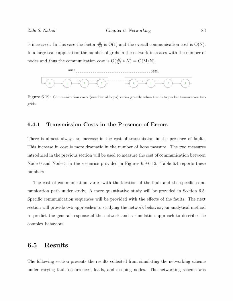
Zahi S. Nakad Chapter 6. Networking 83
is increased. In this case the factor MN2 is O(1) and the overall communication cost is O(N).
In a large-scale application the number of grids in the network increases with the number of
nodes and thus the communication cost is O( MN2 ∗ N) = O(M/N).
0 1 2 3
GRID 0 GRID 1
0 1 2 3
Figure 6.19: Communication costs (number of hops) varies greatly when the data packet transverses two
grids.
6.4.1 Transmission Costs in the Presence of Errors
There is almost always an increase in the cost of transmission in the presence of faults.
This increase in cost is more dramatic in the number of hops measure. The two measures
introduced in the previous section will be used to measure the cost of communication between
Node 0 and Node 5 in the scenarios provided in Figures 6.9-6.12. Table 6.4 reports these
numbers.
The cost of communication varies with the location of the fault and the specific com-
munication path under study. A more quantitative study will be provided in Section 6.5.
Specific communication sequences will be provided with the effects of the faults. The next
section will provide two approaches to studying the network behavior, an analytical method
to predict the general response of the network and a simulation approach to describe the
complex behaviors.
6.5 Results
The following section presents the results collected from simulating the networking scheme
under varying fault occurrences, loads, and sleeping nodes. The networking scheme was
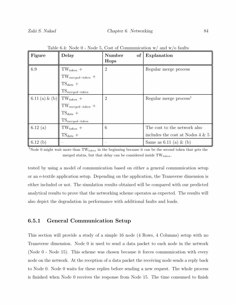
Zahi S. Nakad Chapter 6. Networking 84
Table 6.4: Node 0 - Node 5, Cost of Communication w/ and w/o faults
Figure Delay Number ofHops
Explanation
6.9 TWtoken + 2 Regular merge process
TWmerged−token +
TSdata +
TSmerged−token
6.11 (a) & (b) TWtoken + 2 Regular merge process1
TWmerged−token +
TSdata +
TSmerged−token
6.12 (a) TWtoken + 6 The cost to the network also
TSdata + includes the cost at Nodes 4 & 5
6.12 (b) – – Same as 6.11 (a) & (b)1Node 0 might wait more than TWtoken in the beginning because it can be the second token that gets the
merged status, but that delay can be considered inside TWtoken.
tested by using a model of communication based on either a general communication setup
or an e-textile application setup. Depending on the application, the Transverse dimension is
either included or not. The simulation results obtained will be compared with our predicted
analytical results to prove that the networking scheme operates as expected. The results will
also depict the degradation in performance with additional faults and loads.
6.5.1 General Communication Setup
This section will provide a study of a simple 16 node (4 Rows, 4 Columns) setup with no
Transverse dimension. Node 0 is used to send a data packet to each node in the network
(Node 0 - Node 15). This scheme was chosen because it forces communication with every
node on the network. At the reception of a data packet the receiving node sends a reply back
to Node 0. Node 0 waits for these replies before sending a new request. The whole process
is finished when Node 0 receives the response from Node 15. The time consumed to finish
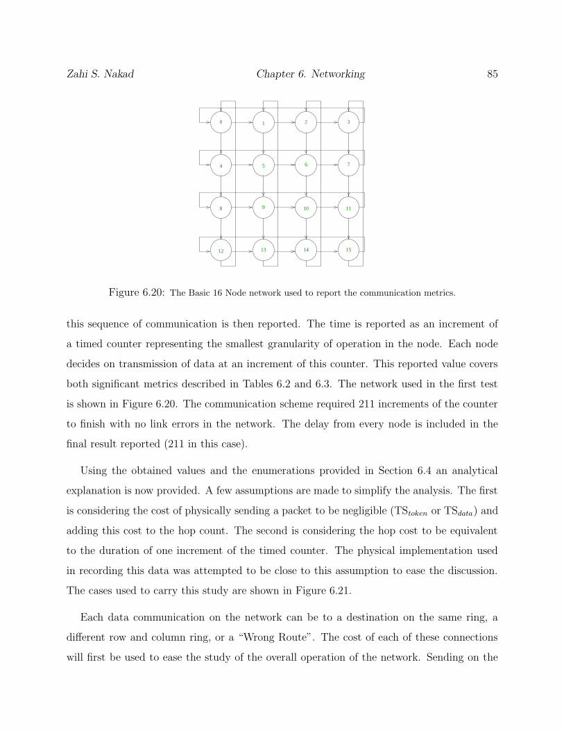
Zahi S. Nakad Chapter 6. Networking 85
0 1 2 3
5 6 7
10 11
13 14 15
8
4
9
12
Figure 6.20: The Basic 16 Node network used to report the communication metrics.
this sequence of communication is then reported. The time is reported as an increment of
a timed counter representing the smallest granularity of operation in the node. Each node
decides on transmission of data at an increment of this counter. This reported value covers
both significant metrics described in Tables 6.2 and 6.3. The network used in the first test
is shown in Figure 6.20. The communication scheme required 211 increments of the counter
to finish with no link errors in the network. The delay from every node is included in the
final result reported (211 in this case).
Using the obtained values and the enumerations provided in Section 6.4 an analytical
explanation is now provided. A few assumptions are made to simplify the analysis. The first
is considering the cost of physically sending a packet to be negligible (TStoken or TSdata) and
adding this cost to the hop count. The second is considering the hop cost to be equivalent
to the duration of one increment of the timed counter. The physical implementation used
in recording this data was attempted to be close to this assumption to ease the discussion.
The cases used to carry this study are shown in Figure 6.21.
Each data communication on the network can be to a destination on the same ring, a
different row and column ring, or a “Wrong Route”. The cost of each of these connections
will first be used to ease the study of the overall operation of the network. Sending on the
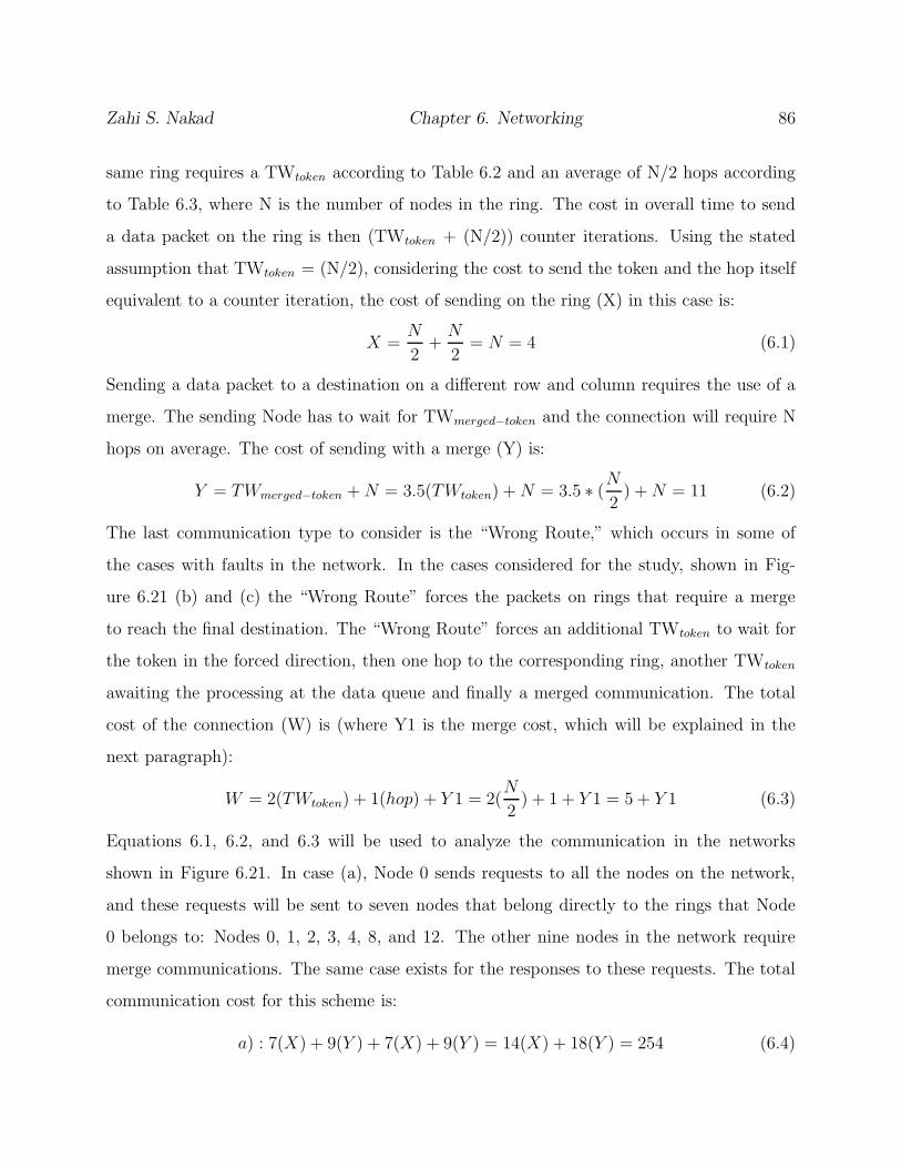
Zahi S. Nakad Chapter 6. Networking 86
same ring requires a TWtoken according to Table 6.2 and an average of N/2 hops according
to Table 6.3, where N is the number of nodes in the ring. The cost in overall time to send
a data packet on the ring is then (TWtoken + (N/2)) counter iterations. Using the stated
assumption that TWtoken = (N/2), considering the cost to send the token and the hop itself
equivalent to a counter iteration, the cost of sending on the ring (X) in this case is:
X =N
2+
N
2= N = 4 (6.1)
Sending a data packet to a destination on a different row and column requires the use of a
merge. The sending Node has to wait for TWmerged−token and the connection will require N
hops on average. The cost of sending with a merge (Y) is:
Y = TWmerged−token + N = 3.5(TWtoken) + N = 3.5 ∗ (N
2) + N = 11 (6.2)
The last communication type to consider is the “Wrong Route,” which occurs in some of
the cases with faults in the network. In the cases considered for the study, shown in Fig-
ure 6.21 (b) and (c) the “Wrong Route” forces the packets on rings that require a merge
to reach the final destination. The “Wrong Route” forces an additional TWtoken to wait for
the token in the forced direction, then one hop to the corresponding ring, another TWtoken
awaiting the processing at the data queue and finally a merged communication. The total
cost of the connection (W) is (where Y1 is the merge cost, which will be explained in the
next paragraph):
W = 2(TWtoken) + 1(hop) + Y 1 = 2(N
2) + 1 + Y 1 = 5 + Y 1 (6.3)
Equations 6.1, 6.2, and 6.3 will be used to analyze the communication in the networks
shown in Figure 6.21. In case (a), Node 0 sends requests to all the nodes on the network,
and these requests will be sent to seven nodes that belong directly to the rings that Node
0 belongs to: Nodes 0, 1, 2, 3, 4, 8, and 12. The other nine nodes in the network require
merge communications. The same case exists for the responses to these requests. The total
communication cost for this scheme is:
a) : 7(X) + 9(Y ) + 7(X) + 9(Y ) = 14(X) + 18(Y ) = 254 (6.4)

Zahi S. Nakad Chapter 6. Networking 87
0 1 2 3
5 6 7
10 11
13 14 15
8
4
9
12
0 1 2 3
5 6 7
10 11
13 14 15
8
4
9
12
0 1 2 3
5 6 7
10 11
13 14 15
8
4
9
12
a) b) c)
Figure 6.21: The general cases for communication with one link errors are shown in b) and c). The link
error in c) belongs to the same ring as Node 0.
6.5.1 Fault Introduction
The following section introduces faults and reports the delay value. The operation of the
whole network with faults is thus scrutinized. The fault tolerant scheme declares a node
unreachable when both its row and column ring are in error. This is a simplistic approach
that only utilizes local error information. This information reports what rings are in error
and not the specific links. The graceful degradation in the performance of the network with
increasing the number of faults will be represented in both the predicted and the simulated
results. This same scheme was tested with one link failure chosen at random for several
different trials. The communication scheme responds differently based on the location of
the faulty link. This difference is attributed to the operation of the networking scheme.
Figure 6.22 shows five trials and the simulated counter value. The two cases presented in
Figure 6.21 (b) and (c) will be used to predict the performance of the networking scheme.
The incremental delays between the one fault cases and the no faults case are the following:
Trial 1: 106, Trial 2: 27, Trial 3: 16, Trial 4: 28, Trial 5: 130. Trial 1 and 5 have a significantly
more severe impact on the operation of the network. Both of these cases have the link error
on a ring that Node 0 (the source of all requests and the destination of all replies in the

Zahi S. Nakad Chapter 6. Networking 88
communication scheme) belongs to. There are two effects to that situation. Node 0 is
creating all the requests and thus all requests destined to a node on the ring with the error
will require a “Wrong Route,” which is usually an expensive operation. When Node 0 is
the destination of all the responses, because this node is on a ring with a link error, every
response has to be dealt with using the fault tolerant scheme (almost always more expensive
than regular operation or at the same cost). When the error is on a ring that Node 0 does
not belong to, such as Trials 2, 3, and 4, the fault tolerant scheme is used in a substantially
smaller portion of the communication and thus the cost is less.
For case (b) in Figure 6.21, Node 0 sends to the same seven nodes directly on the rings.
The six nodes 9, 10, 11, 13, 14, and 15 are again reached using a merged connection. Nodes
5, 6, 7 are also reached through merged connections, but Node 0 has to wait for its row
token to send the merging request; in the other cases it can send either using the row token
or the column token. This increases the initial waiting period. In a regular case the sending
node waits for the token and creates the request; in this case there is probability of 0.5 that
it gets the wrong token first and thus has to wait for another TWtoken. Thus Nodes 5, 6,
7 will have an increment of 0.5(TWtoken), the merge cost Y will be represented by Y1 in
this case where Y1 = Y + 0.5(TWtoken). The seven nodes on the direct rings send back on
those rings. Nodes 9, 10, 11, 13, 14, 15 communicate using regular merging, while Nodes
5, 6, 7 require a “Wrong Route” to reach Row 2 and then a merge to reach Node 0. The
0 1 2 3
5 6 7
10 11
13 14 15
8
4
9
12
0 1 2 3
5 6 7
10 11
13 14 15
8
4
9
12
0 1 2 3
5 6 7
10 11
13 14 15
8
4
9
12
0 1 2 3
5 6 7
10 11
13 14 15
8
4
9
12
0 1 2 3
5 6 7
10 11
13 14 15
8
4
9
12
Counter: 312 Counter: 233 Counter: 222 Counter: 234 Counter: 336Trial: 1 Trial: 2 Trial: 3 Trial: 4 Trial: 5
Figure 6.22: Five trials of one link failures and their respective cost of communication.

Zahi S. Nakad Chapter 6. Networking 89
0 1 2 3
5 6 7
10 11
13 14 15
8
4
9
12
0 1 2 3
5 6 7
10 11
13 14 15
8
4
9
12
0 1 2 3
5 6 7
10 11
13 14 15
8
4
9
12
0 1 2 3
5 6 7
10 11
13 14 15
8
4
9
12
0 1 2 3
5 6 7
10 11
13 14 15
8
4
9
12
Counter: 214 Counter: 336Counter: − Counter: 223Counter: 372Trial: 1 Trial: 2 Trial: 3 Trial: 4 Trial: 5
Figure 6.23: Five trials of two link failures and their respective cost of communication.
communication cost for this case is:
b) : 14(X)+12(Y )+3(Y 1)+3(W ) = 14(X)+15(Y )+3(TWtoken
2)+3(5+Y +1) = 275 (6.5)
For case c), Node 0 sends to Nodes 0, 4, 8, 12 directly on the ring, and to the nine merging
nodes using regular merges with the addition of the extra waiting period because there is
only one merge that is possible. For Nodes 1, 2, and 3, a “Wrong Route” is used; this route
reaches Node 4 and merges are instantiated from there. The responses in this case follow
the same communication routes as the requests and thus the total cost for this case is:
c) : 2(4(X) + 9(Y 1) + 3(W )) = 2(4(X) + 12(Y 1) + 15) = 350 (6.6)
The values calculated using 6.4, 6.5, and 6.6 are representative of the values collected from the
simulator and reported in Figure 6.22. These calculations offer a way to estimate the cost of
communications and to understand the differences in the simulated data. The discrepancies
in the values are attributed to the assumptions taken and probabilities inherent in creating
these enumerations. From the calculated and recorded results, it can be seen that schemes
requiring “Wrong Routes” can increase the cost of communication significantly.
The same general communication scheme was tested with two link errors in the network.
Figure 6.23 presents a portion of the trials tested and the cost values for each case. The
implemented fault tolerant scheme assumes that if a node has an error on its row and column
then that node is unreachable, which is why there is no result for case 3 in Figure 6.23. The
same discussion that applied to the location of the errors in the one fault case applies here.

Zahi S. Nakad Chapter 6. Networking 90
When the fault is on one of the rings of Node 0, the cost increases by a large amount, as
shown by Trials 2 and 4. Since both faults in Trial 4 belong to one ring, then the effect is
the same as that of one link error on that ring. Another point to be added in this discussion
is that the sender will discard any request for a node with an error on its row and column,
Node 4 in Trial 5, for example. This saves on the overall time needed because that request
is never sent. In the case that one error is on a ring connected to Node 0, for example, Row
0 in Trial 2, Node 0 will not learn of the column error on Column 2, and thus will try to
send to Node 2 without discarding the data packet. Node 0 in this case sends to Node 4
using a “Wrong Route”; Node 4 discards the data packet, but Node 0 waits for a timeout
period before it realizes that the connection does not exist. In our case that timeout was set
to 50 counter cycles. Following this analytically, Node 0 requests 0, 4, 8, 12 through ring
connections with cost 4(X), 5, 6, 7, 9, 10, 11, 13, 14, 15 through merges with cost 9(Y1),
and 1, 3 through “Wrong Routes” with cost 2(W), Node 2 costs 50 from the timeout. On
the response a cost of 4(X) from 0, 4, 8, 12; 7(W) from 6, 10, 14, 1, 3 and 6(Y1) from the
remaining nodes. The total cost is (which compares favorably to the cost of 372 obtained
by simulation):
8(X) + 15(Y 1) + 7(W ) + 50 = 381 (6.7)
0 1 2 3
5 6 7
10 11
13 14 15
8
4
9
12
0 1 2 3
5 6 7
10 11
13 14 15
8
4
9
12
0 1 2 3
5 6 7
10 11
13 14 15
8
4
9
12
0 1 2 3
5 6 7
10 11
13 14 15
8
4
9
12
0 1 2 3
5 6 7
10 11
13 14 15
8
4
9
12
Counter: 202 Counter: 233 Counter: 339 Counter: 408 Counter: 402Trial: 1 Trial: 2 Trial: 3 Trial: 4 Trial: 5
Figure 6.24: Five trials of three link failures and their respective cost of communication.
Three fault links in the network have the same effect as previously stated. The effect of the
errors are much larger when on the same ring as Node 0, and there is a larger probability for
timeout cases, for example, Trial 4 and Trial 5 had 2 timeouts each, as shown in Figure 6.24.
The result of Trial 1 is the lowest recorded even though the network has three link errors.

Zahi S. Nakad Chapter 6. Networking 91
0 1 2 3
5 6 7
10 11
13 14 15
8
4
9
12
0 1 2 3
5 6 7
10 11
13 14 15
8
4
9
12
a) b)
Figure 6.25: The two cases with a fabric tear with one surviving link in the tear path.
This is attributed to discarding two request/result pairs at Node 0 (for Nodes 9 and 11).
Table 6.5 provides a summary of the simulation values collected for different fault numbers.
The trials were repeated until clear confidence intervals were reached for the different cases.
For each fault number tested, there are two cases one with a fault occurring on Row 0 or
Column 0 and the other where these rings do not have faults. A few assumptions were used
in representing this data, if more than one fault occur on the same ring, the effect on the
operation of the networking scheme is the same and thus this is considered as one fault and
reported as thus. If Node 0 recognizes that a node has a row and column error and thus does
not send to it, the value 50 (timeout value) was added to the cumulative cost to represent
this loss in connectivity. The reported 95% confidence interval was calculated using [61]:
Mean ± (Standard Deviation)(2.776)√Number of Samples
(6.8)
The reported values manifest the graceful degradation of the networking performance with
the addition of faults.
Tears across the fabric are expected during the operation of an e-textile. The largest
tolerable tear error is one that leaves at least one link in operation as shown in Figure 6.25.
As observed earlier, when the error is on the same ring as Node 0 the communication cost

Zahi S. Nakad Chapter 6. Networking 92
Table 6.5: Summary of Simulation Values (in Counter Increments)
95% Confidence Interval
Case Mean Standard Deviation Lower Bound Upper Bound
1 fault not
on ring1 228.40 5.941 221.04 235.77
1 fault
on ring 321.80 14.37 303.95 339.64
2 faults not
on ring 267 5.29 258.51 275.48
2 faults
on ring 392.5 26.85 355.23 429.76
3 faults not
on ring 302 1 300.39 303.60
3 faults
on ring 459 8.36 447.38 470.611Ring denotes a ring directly attached to Node 0 in this example (Row 0 or Column 0).
is much larger. In this case this increase is more significant because all the communications
outside Column 0 have to use a “Wrong Route”, as shown in Figure 6.25, and this route
has to be pushed down the column three times before it is forwarded, adding a TWtoken at
nodes 4, 8, 12, along with the hop cost.
The costs for the networks shown in Figure 6.26 are 489 for (a) and 225 for (b). This
significant increase is due to Node 0 having to use “Wrong Routes” to reach all the nodes
that are not on Column 0. For case a) Node 0 uses ring connections to send requests to 0,
4, 8, 12. To connect to 13, 14, 15 a “Wrong Route” is used three times to reach Node 12
and then a ring connection. Each “Wrong Route” uses 2 TWtoken and one hop. The cost for
each these connections is 3*2(N/2) + 3 + X. For all other nodes the ring connection from
12 is replaced with a merge of cost Y1. The total cost for requesting is: 4(X) + 3(15 + X)
+ 9(15 + Y1). On the reply side, 1, 4, 8, 12 use a ring connection, thus having a cost of
4(X). 13, 14, 15 use a merge connection 3(Y1). 9, 10, 11 use a “Wrong Route” with one

Zahi S. Nakad Chapter 6. Networking 93
0 1 2 3
5 6 7
10 11
13 14 15
8
4
9
12
0 1 2 3
5 6 7
10 11
13 14 15
8
4
9
12
Figure 6.26: The two cases with a fabric tear with one surviving link in the tear path.
hop and then a merge (Y1), thus having a cost of 3(5 + Y1). 5, 6, 7 use a two hop “Wrong
Route” with a cost of 3(10 + Y1). 1, 2, 3 use the three hop one at a cost of 3(15 + Y1).
The analytical total cost of the network is:
11(X) + 21(Y 1) + 15(15) + 15 + 30 = 566. (6.9)
6.5.2 Increasing the Load
Increasing the load in the network is another important metric. To deal with heavy loads
the work in [15] forced all the nodes to go to merged states when the respective tokens are
captured, and to send on the row-column and column-row rings only. This implementation
of the network deals with light loads, and thus merges will only be asked for when they
are necessary. The topology of this network allows for simultaneous transmissions to take
place at different rings with no effect to the total cost if there is no need for merges. Thus
increasing the load will have no effect on the communication cost of certain communication
schemes (if the communication is restricted inside the rings). The scheme used to test for
communication costs will use the same protocol presented earlier, using a single node to send
requests and wait for replies from all the nodes in the network in a round-robin fashion. To
show the increase in the cost, the method uses multiple nodes to send the same requests
Zahi S. Nakad Chapter 6. Networking 94
Communication Costs with Varying Loads
0
100
200
300
400
500
600
700
1 2 3 4
Number of Requesting Nodes
Counter Iterations
Figure 6.27: The communication cost of the general communication scheme increases significantly while
increasing the number of requesting nodes.
in the same fashion starting with Node 0 and ending in Node 15. For the one sender case,
the value is already reported at 211, where Node 0 was the sender. Three more cases are
presented: two sending nodes (Node 0 and Node 15), three sending nodes (Node 0, Node 15,
and Node 12), and four sending nodes (Node 0, Node 15, Node 12, and Node 3). The reported
cost was as follows: one requesting Node: 211, two requesting Nodes: 260, three requesting
Nodes: 394, four requesting Nodes: 588. These values are plotted in Figure 6.27. This
specific method of increasing the requesting nodes and using these nodes to communicate
with the same destinations was chosen to increase contention and show the degradation in
the response of the networking scheme.
This increase in the cost can be attributed to multiple factors. The first is that when a
node has more than one data packet in its data queue, it only sends one out and thus the
waiting period for the second packet is doubled. Another situation arises when a node (a)
needs to send a data packet on the row, but a merge is already in place and the master of
that merge is circling the row-column token. If node (a) misses sending with this token, the
waiting period is extended (waiting for the column-row to finish circulating and then waiting
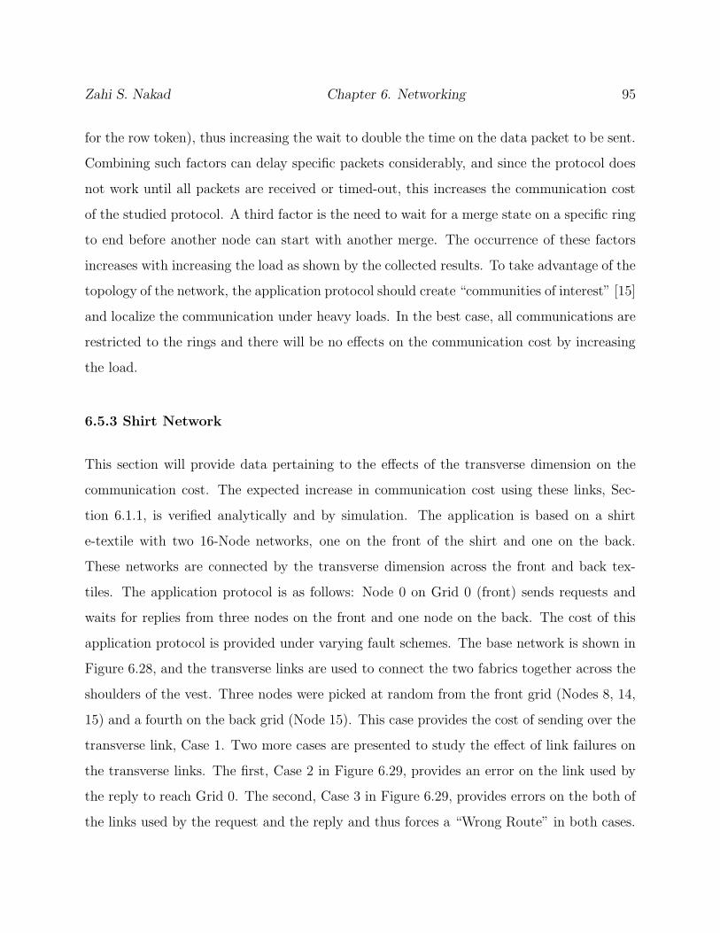
Zahi S. Nakad Chapter 6. Networking 95
for the row token), thus increasing the wait to double the time on the data packet to be sent.
Combining such factors can delay specific packets considerably, and since the protocol does
not work until all packets are received or timed-out, this increases the communication cost
of the studied protocol. A third factor is the need to wait for a merge state on a specific ring
to end before another node can start with another merge. The occurrence of these factors
increases with increasing the load as shown by the collected results. To take advantage of the
topology of the network, the application protocol should create “communities of interest” [15]
and localize the communication under heavy loads. In the best case, all communications are
restricted to the rings and there will be no effects on the communication cost by increasing
the load.
6.5.3 Shirt Network
This section will provide data pertaining to the effects of the transverse dimension on the
communication cost. The expected increase in communication cost using these links, Sec-
tion 6.1.1, is verified analytically and by simulation. The application is based on a shirt
e-textile with two 16-Node networks, one on the front of the shirt and one on the back.
These networks are connected by the transverse dimension across the front and back tex-
tiles. The application protocol is as follows: Node 0 on Grid 0 (front) sends requests and
waits for replies from three nodes on the front and one node on the back. The cost of this
application protocol is provided under varying fault schemes. The base network is shown in
Figure 6.28, and the transverse links are used to connect the two fabrics together across the
shoulders of the vest. Three nodes were picked at random from the front grid (Nodes 8, 14,
15) and a fourth on the back grid (Node 15). This case provides the cost of sending over the
transverse link, Case 1. Two more cases are presented to study the effect of link failures on
the transverse links. The first, Case 2 in Figure 6.29, provides an error on the link used by
the reply to reach Grid 0. The second, Case 3 in Figure 6.29, provides errors on the both of
the links used by the request and the reply and thus forces a “Wrong Route” in both cases.
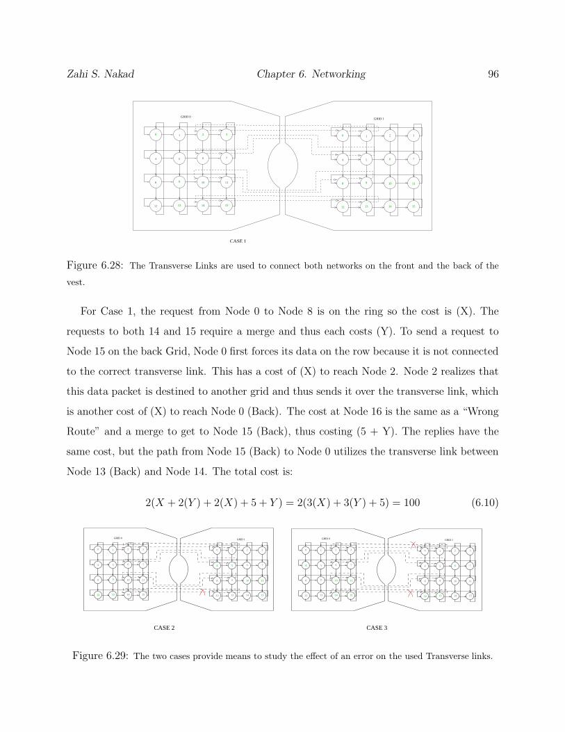
Zahi S. Nakad Chapter 6. Networking 96
0 1 2 3
5 6 7
10 11
13 14 15
8
4
9
12
0 1 2 3
5 6 7
10 11
13 14 15
8
4
9
12
GRID 0GRID 1
CASE 1
Figure 6.28: The Transverse Links are used to connect both networks on the front and the back of the
vest.
For Case 1, the request from Node 0 to Node 8 is on the ring so the cost is (X). The
requests to both 14 and 15 require a merge and thus each costs (Y). To send a request to
Node 15 on the back Grid, Node 0 first forces its data on the row because it is not connected
to the correct transverse link. This has a cost of (X) to reach Node 2. Node 2 realizes that
this data packet is destined to another grid and thus sends it over the transverse link, which
is another cost of (X) to reach Node 0 (Back). The cost at Node 16 is the same as a “Wrong
Route” and a merge to get to Node 15 (Back), thus costing (5 + Y). The replies have the
same cost, but the path from Node 15 (Back) to Node 0 utilizes the transverse link between
Node 13 (Back) and Node 14. The total cost is:
2(X + 2(Y ) + 2(X) + 5 + Y ) = 2(3(X) + 3(Y ) + 5) = 100 (6.10)
0 1 2 3
5 6 7
10 11
13 14 15
8
4
9
12
0 1 2 3
5 6 7
10 11
13 14 15
8
4
9
12
GRID 0 GRID 1
0 1 2 3
5 6 7
10 11
13 14 15
8
4
9
12
0 1 2 3
5 6 7
10 11
13 14 15
8
4
9
12
GRID 0 GRID 1
CASE 2 CASE 3
Figure 6.29: The two cases provide means to study the effect of an error on the used Transverse links.

Zahi S. Nakad Chapter 6. Networking 97
In Case 2, Node 12 (Back) realizes that it cannot use its transverse link and thus forces a
“Wrong Route” on the column, then Node 0 (Back) will route the data to Node 2, at a cost
of X and a W = (4 + 5) = 9. The increase on Case 1 is waiting and one hop = 3. There is
a decrease from the merge to a ring connection (Y - X - W). Then the cost should be 98.
In Case 3, there is one extra hop for the reply since Node 0 (Back) cannot reach the Front
Grid. That is an extra cost of 3 and now the cost is that of a merge plus “Wrong Route”,
thus a total increase of 8. The request in this case too is forced on a “Wrong Route” at Node
3 to Node 7 adding a cost of 3 (waiting and one hop) and the cost of 5 for the “Wrong Route”
processing at Node 4 (Back); thus the total cost should be 108. The simulated values are:
Case 1: 92, Case 2: 81, Case 3: 94. This test presented the increase in the communication
cost by the introduction of Transverse connections.
6.5.4 Sleeping Nodes on a 16-Node Acoustic Beamformer
Inactive nodes in a network can move to a dormant state to lower the power consumption
of the whole network. These sleeping nodes can affect the communication cost since their
effect is the same as two link failures as shown in Figure 6.8. There is no difference between
a sleeping node and a failed node to the routing scheme. The application protocol can be
chosen in a way not to be affected by the sleeping nodes in the system, thus utilizing the
ability to lower the power in the network without the communication costs.
The application protocol provided in this case is the following, where every ring in the
16-Node system represents an Acoustic Array Beamformer. The “master” on each ring will
ask for data from the other nodes and compute a location for the vehicle. The location data
can be verified by checking the data from another ring; in this case the scheme uses a ring
at a perpendicular to the original ring. The communication can thus be constricted to a row
and a column in the system. For specific cases it is assumed that the data is redundant and
only the specific two rings need to be awake in the system. If Node 1 is the node in common
between the two specific rings, the network will be as shown in Figure 6.30.
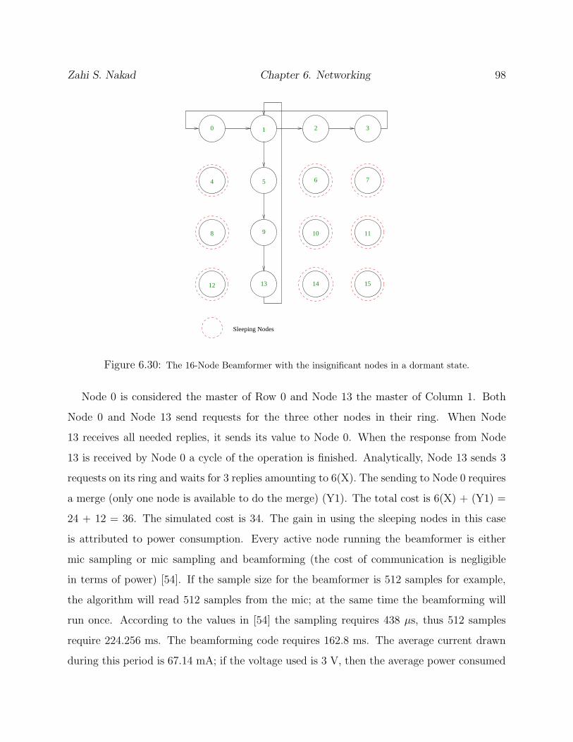
Zahi S. Nakad Chapter 6. Networking 98
0 1 2 3
5 6 7
10 11
13 14 15
8
4
9
12
Sleeping Nodes
Figure 6.30: The 16-Node Beamformer with the insignificant nodes in a dormant state.
Node 0 is considered the master of Row 0 and Node 13 the master of Column 1. Both
Node 0 and Node 13 send requests for the three other nodes in their ring. When Node
13 receives all needed replies, it sends its value to Node 0. When the response from Node
13 is received by Node 0 a cycle of the operation is finished. Analytically, Node 13 sends 3
requests on its ring and waits for 3 replies amounting to 6(X). The sending to Node 0 requires
a merge (only one node is available to do the merge) (Y1). The total cost is 6(X) + (Y1) =
24 + 12 = 36. The simulated cost is 34. The gain in using the sleeping nodes in this case
is attributed to power consumption. Every active node running the beamformer is either
mic sampling or mic sampling and beamforming (the cost of communication is negligible
in terms of power) [54]. If the sample size for the beamformer is 512 samples for example,
the algorithm will read 512 samples from the mic; at the same time the beamforming will
run once. According to the values in [54] the sampling requires 438 µs, thus 512 samples
require 224.256 ms. The beamforming code requires 162.8 ms. The average current drawn
during this period is 67.14 mA; if the voltage used is 3 V, then the average power consumed

Zahi S. Nakad Chapter 6. Networking 99
is 201.42 mW. The power consumption of node in a sleeping mode is negligible and thus the
savings to the system is 201.42 mW x (number of nodes asleep). In this specific example, 9
nodes were asleep and the power consumption is decreased by 1812.78 mW.
Another application scheme is provided in Figure 6.31, Node 0 is the master of Column
0, Node 13 is master of Row 3, and Node 3 of Column 3. The application proceeds as
mentioned earlier with Node 13 and Node 3 sending their information to Node 0. This
application is processed under two routing circumstances, the first considers the sleeping
nodes when communicating between Node 3 and Node 0 and thus routes around the sleeping
nodes (Node 1 & 2) using “Wrong Routes” and a merge. The second wakes up Node 1 and
Node 2 with a token and sends its value directly to Node 0. This application will show the
effects of using the fault tolerance routing on time and power consumption.
In the first case, Node 13 sends its result to Node 0 with a merge at Node 12. Node 3,
sends its result to Node 7, Node 11 and then to Node 15 using “Wrong Routes” after that
a merge at Node 12 relays the message to Node 0. Sending from Node 3 requires more time
and thus it dictates the time required for the application scheme. In the second case, Node
3 wakes Row 0 and sends its data directly to Node 0. In this case the communication from
Node 13 takes more time and dictates the time for the application scheme. The simulation
values collected were 63 for the first case and 58 for the second case. There is a decrease
in time consumed when the sleeping nodes are woken up but at an increase in the power
consumption. Node 1 is awoken at counter increment 28 and Node 2 at 29, this increases the
power consumption by 2 * 201.42mW. Following from the results of this example, there is
a trade-off between power and time consumption that has to be considered for each specific
application.
6.5.2 Conclusion
The implemented networking scheme was discussed in the previous section. This networking
scheme provides connections while dealing with faults and sleeping nodes while degrading

Zahi S. Nakad Chapter 6. Networking 100
Sleeping Nodes
0 1 2 3
5 6 7
10 11
13 14 15
8
4
9
12
Figure 6.31: The 16-Node Beamformer with the insignificant nodes in a dormant state.
gracefully in performance. The simulation results displayed the effects of different situations
on the networking scheme. An analytical method was provided to estimate the communi-
cation cost for specific application protocols. The comparison between the simulated and
the analytical results provide insight into the expected behavior of the networking scheme.
This analytical method introduces more errors as it analyzes a longer time as can be seen
in Figure 6.32 representing the simulation times versus the analytical times predicted. As
a general statement, faults in the network increase the communication cost by changing a
route to a more expensive one, a ring connection to a merge or “Wrong Route” (X → Y or
W), or a merge connection to a “Wrong Route” (Y → W), for example.
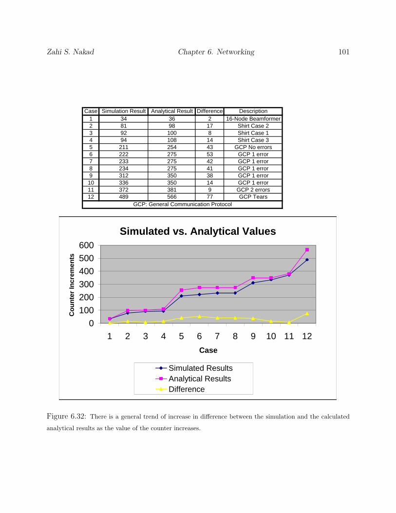
Zahi S. Nakad Chapter 6. Networking 101
Case Simulation Result Analytical Result Difference Description1 34 36 2 16-Node Beamformer2 81 98 17 Shirt Case 23 92 100 8 Shirt Case 14 94 108 14 Shirt Case 35 211 254 43 GCP No errors6 222 275 53 GCP 1 error7 233 275 42 GCP 1 error8 234 275 41 GCP 1 error9 312 350 38 GCP 1 error10 336 350 14 GCP 1 error11 372 381 9 GCP 2 errors12 489 566 77 GCP Tears
GCP: General Communication Protocol
Simulated vs. Analytical Values
0
100
200
300
400
500
600
1 2 3 4 5 6 7 8 9 10 11 12
Case
Co
un
ter
Incr
emen
ts
Simulated ResultsAnalytical ResultsDifference
Figure 6.32: There is a general trend of increase in difference between the simulation and the calculated
analytical results as the value of the counter increases.

Chapter 7
Conclusion
The major goal of this research was to create an electronic textile architecture that embodies
the experience gained from constructing hardware prototypes, provides the framework for
a simulation environment for e-textile systems, and maps future directions for the e-textile
architecture. This goal was reached by developing a set of precepts to govern future endeavors
and to guide the process of creating e-textile applications.
Three main areas of precepts, embedding of conductive channels, manufacturing, and
software, were presented in Chapter 4. The listed precepts provide the basis of an evolv-
ing electronic textiles architecture. The precept discussions provided details on previous
attempts and failures along with foreseen future directions. As an example, the developed
precepts recommend the use of digital communication through insulated wires governed by a
fault-tolerant low-power communication scheme. More experience and experimentation will
develop these precepts from open-ended guidelines to a more established set of precise rules.
The process of formulating the precepts based upon acquired experience helped in the
creation of the software environment that acts as a simulation and evaluation toolkit for
hardware prototypes. This environment can be used at the outset of a project to test the
feasibility and make design decisions. The simulation process will later help in fine-tuning
102

Zahi S. Nakad Chapter 7. Conclusion 103
the created hardware by varying system parameters, which is easier in the virtual world.
The research done in [54] augmented this simulator with a power consumption and fabric
fault simulator, while the work in [53] dealt with creating an acoustic data and beamformer
algorithm simulator; the simulator was discussed in Chapter 5. This simulation also aids in
exploring the design space of e-textiles. This design space is too large to be explored with
only hardware prototypes. The simulation environment provides the ability to simulate both
the sensed environment and the response of the e-textile system.
Providing low-power fault-tolerant communication between separate nodes on an e-textile
is a must. The creation and testing of such a networking scheme was made possible using
the simulation environment. Testing and developing this networking scheme was only possi-
ble in the simulation environment due to the limited number of hardware prototype nodes.
Chapter 6 presented the theory, operation, analysis, and simulation results of this networking
scheme. The presented networking scheme provides connectivity in the presence of faults.
Faults are expected on an e-textile during manufacturing and deployment. Low-power op-
eration requires the use of sleeping modes in the processing nodes on an e-textile to save on
power. The networking scheme provides support to these sleeping nodes by offering alternate
routes to keep these nodes in the sleeping mode. The performance of this network can be
accurately predicted using the analytical method discussed in Chapter 6.
Finally, a 30-foot Acoustic Beamforming Array was created to test the theories and the
precepts. This e-textile detects the presence and the line of bearing of a large vehicle using
acoustic beamforming. The triangulation of the computed line of bearing from four au-
tonomous clusters provides location data for the sensed vehicle. This is the first e-textile to
include computing and networking on the fabric. This work helped in moving forward the
evolution of the electronic textiles architecture.
The contributions of this dissertation work are summarized in the following list:
- Definition of an electronic textile architecture by creating architectural precepts based
on experience and on-going research (Chapter 4)

Zahi S. Nakad Chapter 7. Conclusion 104
- Creation of a simulation environment to test new concepts and improve extant proto-
types using the Ptolemy environment (Chapter 5)
- Development of a networking scheme that routes around faults and sleeping nodes with
predictable performance (Chapter 6)
- Implementation of the acoustic beamforming array as the first e-textile hardware pro-
totype that combines sensing and processing on the fabric (Section 3.4)
The future directions foreseen for this architecture can be divided into immediate issues
and general paths. The immediate issues include creating fabric/electronics connections to
provide for easier and more stable connections of components, integration of fiber and thin-
film form components in the prototypes, and experimentation with different weave patterns
and conductive channels.
The general paths encompass the creation of a more thorough electronic textiles archi-
tecture. The general open-ended precepts reported in Chapter 4 should be developed after
thorough research into a set of specific rules to manage all the details of creating elec-
tronic textile systems. Design paths should focus on creating more general nodes and fabric
swatches to take advantage of mass producing the electronic components and the fabric
backplanes to lower the cost of these systems and minimize re-invention. To fully exploit the
low cost manufacturing of textiles, the design of e-textile systems should correspond to the
extant fabric manufacturing techniques. The generality in design should cover all aspects
of e-textile research and conform to the created precepts. Future research endeavors should
focus towards the deeper establishment of the general electronic textile architecture.
The presentation of the software architecture should be in a more user-oriented fashion.
The software should provide services based on the precepts and algorithms given in this dis-
sertation. The use of these services will inherently force the implementation of the developed
rules, facilitating the design process and minimizing re-invention.

Bibliography
[1] Promatech web site, http://www.promatech.it.
[2] R. Parker, R. Riley, M. Jones, D. Leo, L. Beex, and T. Milson, “STRETCH - An E-
Textile for Large-Scale Sensor Systems,” International Interactive Textiles for the Warrior
Conference, July 2002, Abstract for poster presentation, pp. 59.
[3] M. Jones, T. Martin, and Z. Nakad, “A Service Backplane for E-Textile Applica-
tions,” Workshop on Modeling, Analysis, and Middleware Support for Electronic Textiles
(MAMSET), October 2002.
[4] E.R. Post, M. Orth, P.R. Russo, and N. Gershenfeld, “E-broidery Design and fabrication
of textile-based computing,” IBM Systems Journal, Vol. 39, Nos. 3&4, 2000.
[5] D. Marculescu, R. Marculescu, and P.K. Khosla, “Challenges and Opportunities in elec-
tronic textiles modeling and optimization,” Proceedings of the 39th Design Automation
Conference, pp. 175-180, 2002.
[6] B. Firoozbakhsh, N. Jayant, S. Park, and S. Jayaraman, “Wireless Communication of
Vital Signs Using the Georgia Tech Wearable Motherboard,” 2000 IEEE Conference on
Multimedia and Expo (ICME 200), pp. 1253 - 1256, vol. 3, 30 July - 2 Aug 2000.
[7] Measurement Specialties Inc. website, http://www.msiusa.com.
[8] B.C. Kim, G.M. Spinks, G.G. Wallace, and R. John, “Electroformation of conductive
polymers in a hydrogel support matrix,” Polymer 2000.
105
Zahi S. Nakad Bibliography 106
[9] W. Wolf, “A Decade of Hardware/Software Codesign,” Computer, Vol. 36, No. 4, pp.
38-43, April 2003.
[10] B. Akle and D. Leo, “Multilayer ionic transducers,” Proceedings of the 2003 SPIE annual
conference,”
[11] R.A. Riley,Jr., S.B. Thakkar, J.P. Czarnaski, and B. Schott, “Power-Aware Acoustic
Beamforming,” Proceedings of the Fifth International Military Sensing Symposium, De-
cember 2002.
[12] T.D. Todd, “The Token Grid: Multidimensional Media Access For Local and Metropoli-
tan Networks,” Eleventh Annual Joint Conference of the IEEE Computer and Commu-
nications Societies, INFOCOM ‘92.
[13] E.L. Hahne and T.D. Todd, “Fault-Tolerant Multimesh Networks,” Global Telecommu-
nications Conference, GLOBECOM ‘92.
[14] T.D. Todd and E.L. Hahne, “Multiaccess Mesh (Multimesh) Networks,” IEEE/ACM
Transactions on Networking, April 1997.
[15] T.D. Todd, “The Token Grid Network,” IEEE/ACM Transactions on Networking, June
1994.
[16] K. Hwang, Advanced Computer Architecture: Parallelism, Scalability, Programmability.
McGraw-Hill Series in Computer Science, 1993.
[17] OPNET Technologies, Inc. Software That Understands Networks. OPNET Optimum
Network Performance. http://www.opnet.com.
[18] Ptolemy Project, Heterogeneous Modeling and Design. UC Berkeley, EECS. http:
ptolemy.eecs.berkeley.edu.
[19] Edward E. Lee, “Overview of the Ptolemy Project,” Technical Memorandum UCB/ERL
M01/11, March 2001.

Zahi S. Nakad Bibliography 107
[20] David K. Cambell, Adaptive Beamforming Using a Microphone Array for Hands-Free
Telephony. Master’s Thesis, Virginia Polytechnic Institute and State University, 1999.
[21] S. Basu, S. Schwarz, and A. Pentland, “Wearable Phased Arrays for Sound Localization
and Enhancement,” The Fourth International Symposium on Wearable Computers, 2000.
[22] F. Khalil, J. Jullien, and A. Gilloire, “Microphone Array for Sound Pickup in Telecon-
ference Systems,” J. Audio Eng. Soc., Vol. 42, No. 9, 1994 September.
[23] ElekSen Ltd., http://www.electrotextiles.com.
[24] Technology Backgrounder, Press Information ElekTexTM Switching and Sending Fab-
ric, http://www.electrotextiles.com/flash/tech spec.shtml.
[25] Sterling Performance Fibers, Conductrol. http://www.sterlingfibers.com.
[26] Guilford Technical Textiles, STAT STAR. http://www.guilfordmills.com.
[27] Bekintex, A Member Of The Bekaert Group, http://www.bekintex.com.
[28] B. Howard and S. Howard, “Lightglove: Wrist-Worn Virtual Typing and Pointing,”
Fifth International Symposium on Wearable Computers, 2001.
[29] D.D. Rossi, F. Lorussi, A. Mazzoldi, and E.P. Scilingo, “Active Dressware: Wearable
Proprioceptive Systems Based on Electroactive Polymers,” Fifth International Sympo-
sium on Wearable Computers, 2001.
[30] S. Nakamura, M. Tsukamoto, and S. Nishio, “A Method of Key Input with Two Mice,”
Fifth International Symposium on Wearable Computers, 2001.
[31] J. Rekimoto, “GestureWrist and GesturePad: Unobtrusive Wearable Interaction De-
vices,” Fifth International Symposium on Wearable Computers, 2001.
[32] J. Edmison, M. Jones, Z. Nakad, and T. Martin, “Using Piezoelectric Materials for
Wearable Electronic Textiles,” Proceedings of the Sixth International Symposium on
Wearable Computers, 2002.

Zahi S. Nakad Bibliography 108
[33] MIThril: MIThril, the next generation research platform for context aware wearable
computing. http://www.media.mit.edu/wearables/mithril.
[34] E.J. Lind, S. Jayaraman, R. Eisler, and T. McKee, “A Sensate Liner for Personnel
Monitoring Applications,” First International Symposium on Wearable Computers, 1997.
[35] Princeton University, Macroelectronics Group. http://www.ee.princeton.edu/∼asg.
[36] Ultralife Batteries INC, The New Power Generation. http://www.ulbi.com.
[37] InfinitePowerSolutions, About LiTE*STAR, http://www.infinitepowersolutions.com/
technology/about-lite-star.htm.
[38] NC State University, College of Textiles for Research.
http://www.tx.ncsu.edu/research list/sponsor search.cfm?sponsor=MCNC.
[39] Iowa Thin Film Technologies. http://www.iowathinfilm.com.
[40] K.V. Laerhoven and O. Cakmakci, “What Shall We Teach Our Pants,” Fourth Inter-
national Symposium on Wearable Computers, 2000.
[41] Jonny Farringdon, Andrew J. Moore, Nancy Tilbury, James Church, and
Pieter D. Biemond, “Wearble Sensor Badge and Sensor Jacket for Context Awarness,”
Third International Sysmposium on Wearable Computers (ISWC 1999), pp. 107 - 113,
Oct. 1999.
[42] Andrew R. Golding and Neal Lesh, “Indoor navigations using a diverse set of cheap,
wearable sensors,” Proceedings of the Third International Symposium on Wearable Com-
puting (ISWC 1999), pp. 29 - 36, Oct. 1999.
[43] P.G. Tortora, B.J. Collier, Understanding Textiles. Prentice Hall, 1997.
[44] Diana Marculescu, Radu Marculescu, Nicholas H. Zamora, Phillip Stanley-Marbell,
Pradeep K. Kholsa, Sungmee Park, Sundaresan Jayaraman, Stefan Jung, Christl Lauter-
bach, Werner Weber, Tunde Kirstein, Didier Cottet, Janusz Grzyb, Gerhard Troster,
Zahi S. Nakad Bibliography 109
Mark Jones, Tom Martin, and Zahi Nakad, “Electronic Textiles: A Platform for Perva-
sive Computing,” Proceedings of the IEEE, Vol. 91, No. 12, 2003.
[45] Tessera website, http://www.tessera.com.
[46] M. Jones, T. Martin, Z. Nakad, R. Shenoy, T. Sheikh, D. Lehn, and J. Edmison, “Ana-
lyzing the Use of E-textiles to Improve Application Performance,” IEEE Vehicular Tech-
nology Conference 2003, Symposium on Wireless Adhoc, Sensor, and Wearable Networks
(VTC 2003), Oct. 2003.
[47] Bernina website, http://www.berninausa.com.
[48] Brother webiste, http://www.brother.com.
[49] 3M website, 3M Worldwide, Innovative and Practical Solutions from a Diversified Tech-
nology Company, http://www.3m.com.
[50] T. Marin, M. Jones, J. Edmison, and R. Shenoy, “Towards a design framework for
wearable electronic textiles,” Seventh International Symposium on Wearable Computers
(ISWC 2003), Oct. 2003.
[51] D. Lehn, C. Neely, K. Schoonover, T. Martin, and M. Jones, “e-TAGS: e-Textile At-
tachment Gadgets,” Second IEEE International Conference on Pervasive Computing and
Communications (PerCom 2004), March 2004 (submitted).
[52] Phillips Semiconductors, “The I2C-BUS Specification, Version 2.1, January 2000,”
http://www.semiconductors.philips.com/acrobat/literature/9398/39340011.pdf.
[53] Ravi R. Shenoy, “Design of e-textiles for acoustic applications,” Master’s Thesis, Vir-
ginia Polytechnic Institute and State University, 2003.
[54] Tanwir Sheikh, “Modeling of Power Consumption and Fault Tolerance for Electronic
Textiles,” Master’s Thesis, Virginia Polytechnic Institute and State University, 2003.
Zahi S. Nakad Bibliography 110
[55] Analog Devices, “DSP Microcomputer, ADSP-2188M,”
http://www.analog.com/productSelection/pdf/ADSP-2188M 0.pdf.
[56] Internal Lab Communication with David I. Lehn.
[57] CMU Graphics Lab Motion Capture Database, http://mocap.cs.cmu.edu/search.html.
[58] Sun Microsystems, Java Native Interface, http://java.sun.com/j2se/1.3/docs/guide/jni/.
[59] Z. Nakad, M. Jones, and T. Martin, “Communications in Electronic Textile Systems,”
The 2003 International Conference on Communications in Computing (CIC 2003), June
2003.
[60] World Wide Web Consortium, Extensible Markup Language (XML),
http://www.w3.org/XML/.
[61] Raj Jain, The Art Of Computer Systems Performance Analysis: Techniques for Ex-
perimental Design, Measurement, Simulation, and Modeling. John Wiley & Sons, Inc.
1991.
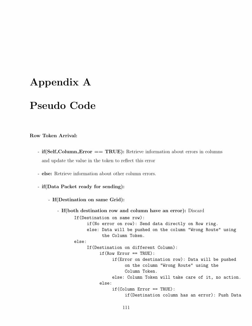
Appendix A
Pseudo Code
Row Token Arrival:
- if(Self Column Error == TRUE): Retrieve information about errors in columns
and update the value in the token to reflect this error
- else: Retrieve information about other column errors.
- if(Data Packet ready for sending):
- If(Destination on same Grid):
- If(both destination row and column have an error): Discard
If(Destination on same row):
if(No error on row): Send data directly on Row ring.
else: Data will be pushed on the column "Wrong Route" using
the Column Token.
else:
If(Destination on different Column):
if(Row Error == TRUE):
if(Error on destination row): Data will be pushed
on the column "Wrong Route" using the
Column Token.
else: Column Token will take care of it, no action.
else:
if(Column Error == TRUE):
if(Destination column has an error): Push Data
111

Zahi S. Nakad Appendix A 112
down the row "Wrong Route".
else: Ask for a merger with this Row and
Destination Column.
else:
if(Destination column has an error):
if((Error on this Column)||
(Error on Destination Row)):
Push Data down the row "Wrong Route".
else: Return to Data Queue for
later processing.
else: (all good): Ask for a merger with this
Row and Destination Column.
else:
if(Column Error == TRUE): Push Data down the row
"Wrong Route".
else: Column Token will take care of it.
- else: Transverse Token will take care of it, no action.
- else: No Action
- If(Waiting For Row Token == 1):
- //Column Token has been captured
- Create a Row Column Token
- Merged Status = 1;
- Waiting For Row Token = 0;
- Send Token on Row ring.
- If(Merged Status == 0):
- If this node was asked to go to a merged state:
- Grab the token
- Waiting For Column Token = 1;
- else: Release the Row Token on the Row ring.
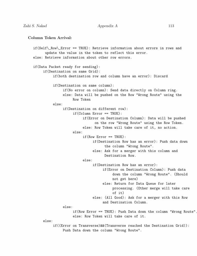
Zahi S. Nakad Appendix A 113
Column Token Arrival:
if(Self\_Row\_Error == TRUE): Retrieve information about errors in rows and
update the value in the token to reflect this error.
else: Retrieve information about other row errors.
if(Data Packet ready for sending):
if(Destination on same Grid):
if(both destination row and column have an error): Discard
if(Destination on same column):
if(No error on column): Send data directly on Column ring.
else: Data will be pushed on the Row "Wrong Route" using the
Row Token
else:
if(Destination on different row):
if(Column Error == TRUE):
if(Error on Destination Column): Data will be pushed
on the row "Wrong Route" using the Row Token.
else: Row Token will take care of it, no action.
else:
if(Row Error == TRUE):
if(Destination Row has an error): Push data down
the column "Wrong Route".
else: Ask for a merger with this column and
Destination Row.
else:
if(Destination Row has an error):
if(Error on Destination Column): Push data
down the column "Wrong Route". (Should
not get here)
else: Return for Data Queue for later
processing. (Other merge will take care
of it)
else: (All Good): Ask for a merger with this Row
and Destination Column.
else:
if(Row Error == TRUE): Push Data down the column "Wrong Route".
else: Row Token will take care of it.
else:
if((Error on Transverse)&&(Transverse reached the Destination Grid)):
Push Data down the column "Wrong Route".

Zahi S. Nakad Appendix A 114
else:
if((Error on Row)&&(Transverse cannot reach the Destination Grid)):
Push data down the column "Wrong Route".
else: keep the data for later processing by other tokens.
- If(Waiting For Column Token == 1):
- //Row Token has been captured
- Create a Row Column Token
- Merged Status = 1;
- Waiting For Column Token = 0;
- Send Token on Row ring.
- If(Merged Status == 0):
- If this node was asked to go to a merged state:
- Grab the token
- Waiting For Row Token = 1;
- else: Release the Column Token on the Column ring.
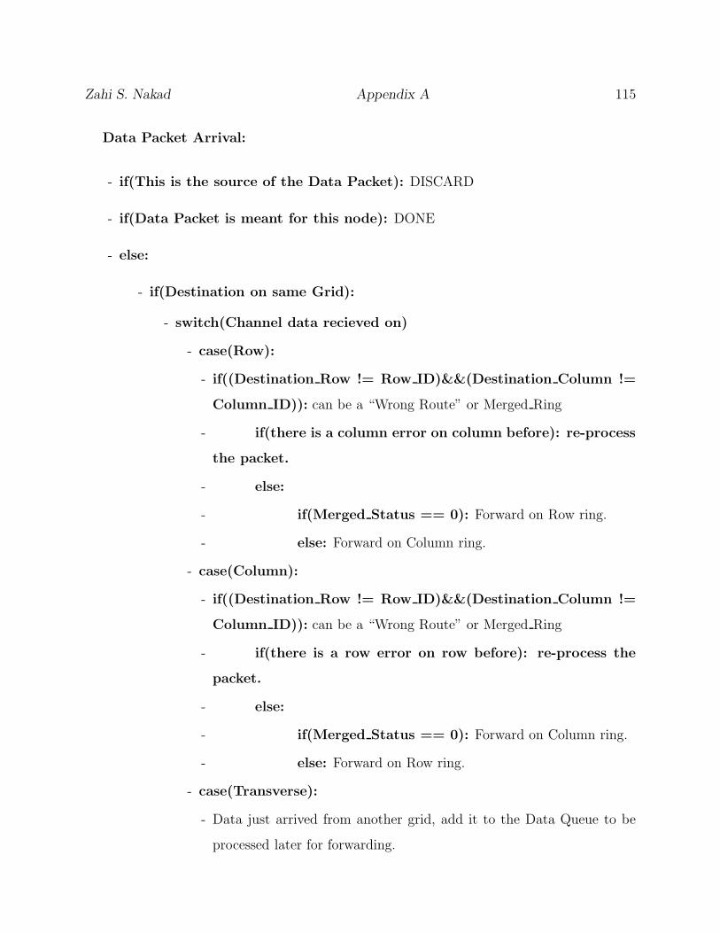
Zahi S. Nakad Appendix A 115
Data Packet Arrival:
- if(This is the source of the Data Packet): DISCARD
- if(Data Packet is meant for this node): DONE
- else:
- if(Destination on same Grid):
- switch(Channel data recieved on)
- case(Row):
- if((Destination Row != Row ID)&&(Destination Column !=
Column ID)): can be a “Wrong Route” or Merged Ring
- if(there is a column error on column before): re-process
the packet.
- else:
- if(Merged Status == 0): Forward on Row ring.
- else: Forward on Column ring.
- case(Column):
- if((Destination Row != Row ID)&&(Destination Column !=
Column ID)): can be a “Wrong Route” or Merged Ring
- if(there is a row error on row before): re-process the
packet.
- else:
- if(Merged Status == 0): Forward on Column ring.
- else: Forward on Row ring.
- case(Transverse):
- Data just arrived from another grid, add it to the Data Queue to be
processed later for forwarding.

Zahi S. Nakad Appendix A 116
- else:
- if Data received on Transverse ring: Forward Data on Transverse
- else: Let the Transverse Token deal with forwarding this packet.

Vita
Zahi Nakad was born in the winter of 1976 in a small town called Jdita in the Bekaa Valley,
Lebanon. After graduating from his high school, he was accepted to the Computer and
Communication Engineering program at the American University of Beirut. After graduating
with distinction in 1998, Zahi joined the Computer Engineering program in the Bradley
Department of Electrical and Computer Engineering at Virginia Tech as a graduate student.
In the spring of 1999, Zahi joined the Configurable Computing Lab and received his Master’s
degree in 2000 under the guidance of Dr. Mark Jones. Zahi’s work then focused on e-
textiles and creating the VT e-Textiles Group in the Configurable Computing Lab under
the guidance of Dr. Mark Jones and Dr. Thomas Martin. He received his Ph.D. degree in
Computer Engineering in 2003.
117