
Architectures and Algorithms for Resource Allocation Mounire El Houmaidi *, Mostafa A. Bassiouni *,...
20
Architectures and Architectures and Algorithms for Resource Algorithms for Resource Allocation Allocation Mounire El Houmaidi Mounire El Houmaidi * , Mostafa A. Bassiouni , Mostafa A. Bassiouni * , and Guifang Li , and Guifang Li # * School of Electrical Engineering and Computer Science School of Electrical Engineering and Computer Science # School of Optics/CREOL School of Optics/CREOL University of Central Florida University of Central Florida
-
date post
21-Dec-2015 -
Category
Documents
-
view
218 -
download
0
Transcript of Architectures and Algorithms for Resource Allocation Mounire El Houmaidi *, Mostafa A. Bassiouni *,...

Architectures and Algorithms for Architectures and Algorithms for Resource AllocationResource Allocation
Mounire El HoumaidiMounire El Houmaidi**, Mostafa A. Bassiouni, Mostafa A. Bassiouni**, and Guifang Li, and Guifang Li##
**School of Electrical Engineering and Computer ScienceSchool of Electrical Engineering and Computer Science##School of Optics/CREOLSchool of Optics/CREOL
University of Central FloridaUniversity of Central Florida
OutlineOutline Motivation What is a Minimum Dominating Set (MDS) How to find k-MDS
– Algorithm– Example– What is Weighted MDS
Applications of k-MDS– Sparse placement of wavelength conversion
• k-LOSS(k-BLK) and F-SEARCH• Weighted k-MDS for non-uniform traffic• Limited wavelength conversion
– Placement of G-nodes for traffic grooming– Placement of FDLs
Conclusions

Motivation- Resource placementMotivation- Resource placement
Optimize overall network performance by using dominating nodes [1-4]
1. M. El Houmaidi et. al., J. Opt. Net., 2:6, (OSA, 2003)2. M. El Houmaidi et. al., Proc. MASCOTS, (IEEE/ACM, 2003)3. M. El Houmaidi et. al., J. Opt. Eng., 43:1, (SPIE, 2004) 4. M. El Houmaidi et. al., Proc. OFC, (IEEE, 2004)
1
0
2
3
4
5
6
7
8
10
9
11
13
12
14
15
16
17
18
19
20
21
22
23
24
25
26
27
(U.S Long Haul Net.)
What is What is MDSMDS Given a graph G(V,E), determine a set with minimum
number of vertices D V such that every vertex in the graph is either in D or is at distance k or less from at least one member in D.
NP-Complete problem [1,2] .
Heuristic algorithms for sub-optimal solution.
Highly connected nodes dominate the entire topology.
1. Karp, Pl. Press, 19722. Lund, et. al., J. ACM, 1994
DefinitionsDefinitions
Neighbor (v): is the set of nodes sharing a link with v.
k-Neighbor (v): is the set of nodes that are at most within k hops away from a node v.
For k equals 0, 0-Neighbor(v) contains the node v only.

Definitions (Cont.)Definitions (Cont.) k-Connect(v): the connectivity index based on nodes within k hops of v is :
k-Master (v): represents the node p, member of k-Neighbor(v), with the highest k-Connect value over all nodes m that are at most k hops away from node v (i.e., all nodes mk-Neighbor(v))
)Neighbor(v m
(m) Connect-1)-(k + (v) Connect-1)-(k = (v) Connect-k
:as (v) Connect-k define y weRecursivel
)Neighbor(v m(m) Connect-0 + (v) Connect-0 = (v) Connect-1
(v)) (Neighbory Cardinalit = (v) Degree = (v) Connect-0
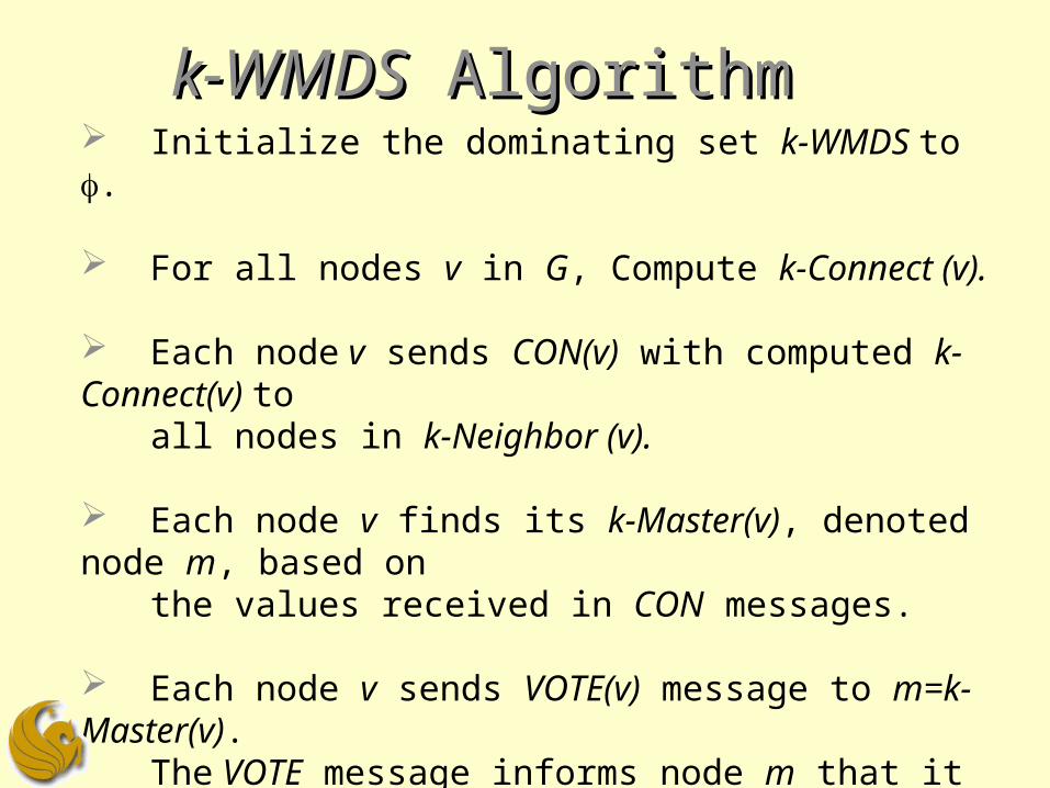
k-WMDSk-WMDS Algorithm Algorithm Initialize the dominating set k-WMDS to .
For all nodes v in G, Compute k-Connect (v).
Each node v sends CON(v) with computed k-Connect(v) to all nodes in k-Neighbor (v).
Each node v finds its k-Master(v), denoted node m, based on the values received in CON messages.
Each node v sends VOTE(v) message to m=k-Master(v). The VOTE message informs node m that it is a master node .
Each node that receives VOTE(v) adds itself to k-WMDS.
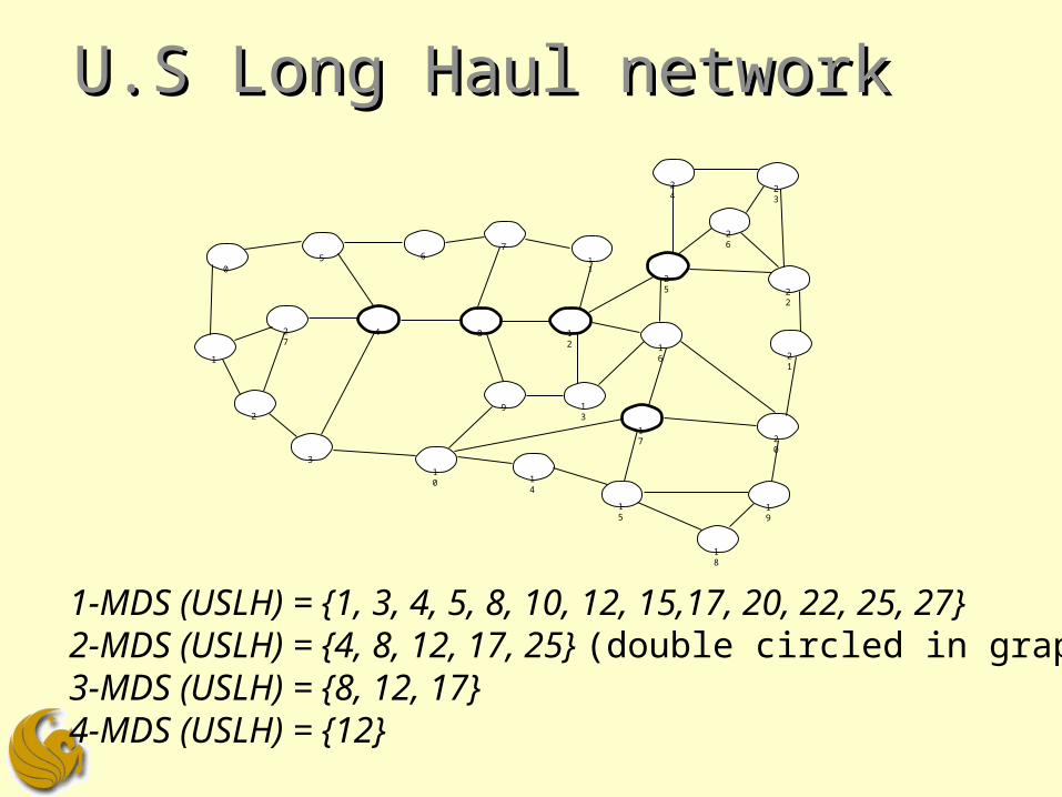
U.S Long Haul networkU.S Long Haul network
1-MDS (USLH) = {1, 3, 4, 5, 8, 10, 12, 15,17, 20, 22, 25, 27} 2-MDS (USLH) = {4, 8, 12, 17, 25} (double circled in graph)3-MDS (USLH) = {8, 12, 17}4-MDS (USLH) = {12}
1
0
2
3
4
5
6
7
8
10
9
11
13
12
14
15
16
17
18
19
20
21
22
23
24
25
26
27
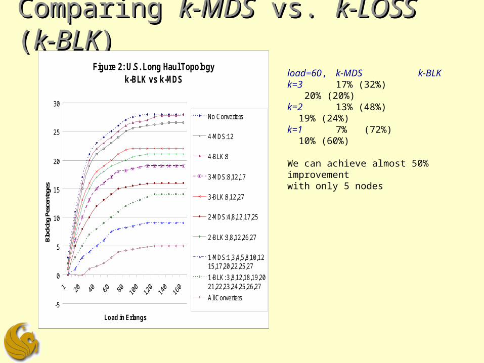
Comparing Comparing k-MDSk-MDS vs. vs. k-LOSS k-LOSS ((k-BLKk-BLK))Figure 2: U.S. Long Haul Topology
k-BLK vs k-MDS
-5
0
5
10
15
20
25
30
Load in Erlangs
Blo
ckin
g Pe
rcen
tage
s
No Converters
4-MDS:12
4-BLK:8
3-MDS:8,12,17
3-BLK:8,12,27
2-MDS:4,8,12,17,25
2-BLK:3,8,12,26,27
1-MDS:1,3,4,5,8,10,1215,17,20,22,25,27
1-BLK: 3,8,12,18,19,2021,22,23,24,25,26,27
All Converters
load=60, k-MDS k-BLKk=3 17% (32%) 20% (20%)k=2 13% (48%) 19% (24%) k=1 7% (72%) 10% (60%)
We can achieve almost 50% improvement with only 5 nodes

Weighted Weighted MDSMDS ( (k-WMDSk-WMDS))
1-WMDS (NSF) = {1, 4, 5, 6, 9, 11, 14}2-WMDS (NSF) = {1, 4, 9, 14}
3-WMDS (NSF) = {14}
1
0
2
3
4
5
6
7
8
10
9
11
13
12
14
15
NSFNET: nationwide backbone network
0-Connect (v) = Cardinality (Neighbor (v)) * Weight(v)

k-LOSS (k-BLK) k-LOSS (k-BLK) vsvs. k-WMDS. k-WMDS Figure 6: NSFNET topology
k-BLK vs k-WMDS
0
5
10
15
20
25
30
35
40
1 10 20 30 40 50 60 70 80 90 100
Load in Erlangs
Bloc
king
Per
cent
ages
No Converters
3-WMDS:14
3-BLK:5
2-WMDS:1,4,9,14
2-BLK:5,4,15,14
1-WMDS:1,4,5,6,9,11,14
1-BLK:5,4,15,14,13,12,11
All Converters
Under a load of 70, we simulated non-uniform traffic pattern between node pairs:
Node Weight0 61 122 73 124 55 86 17 118 79 210 711 1512 313 1514 915 2

Placement of Limited OWCPlacement of Limited OWC
Figure 6: U.S Long Haul LIMITED vs F-SEARCH (50 Erlang, W=8)
0
5
10
15
20
25
Number of wavelength Converters
Bloc
king
Per
cent
age
F-S:Flexible Node-Sharing
LIM:Flexible Node-Sharing
Figure 8: U.S Long Haul LIMITED vs F-SEARCH (50 Erlang, W=8)
0
5
10
15
20
25
30
Number of wavelength ConvertersBl
ocki
ng P
erce
ntag
e
F-S:Static Mapping
LIM:Static Mapping
LIMITED has better performance than F-SEARCH for Flexible node-sharing and Static mapping optical switch designs.

G-nodes placement: T-G-nodes placement: T-GroomingGrooming
NSF Network (W=8)
0
10
20
30
40
50
60
70
80
Load in Erlangs
Net
wo
rk T
hro
ug
hp
ut
Full Grooming
1-WMDS
1-BLK
2-WMDS
2-BLK
3-WMDS
3-BLK
No Grooming
NSFNET topology (W=8)
0
10
20
30
40
50
60
70
80
Load in Erlangs
Net
wo
rk T
hro
ug
hp
ut
2-WMDS: r=16
2-BLK: r=16
2-WMDS: r=8
2-BLK: r=8
We can achieve with 2-WMDS members as G-nodes (r=16) the same throughput as if all nodes in the network had the grooming capability (r is the grooming ratio)

OBS switch design with FDLs/OWCsOBS switch design with FDLs/OWCs
Input Link 2
DMX
MUX
MAIN CONTROL
DMX: De-multiplexor
MUX: Multiplexor
OWC: any-to- Converter
FDL: Fiber Delay Line
DMX
MUX
1
W
F.W
1
W
i O X C
Output Link 1
Output Link 2
Input Link 1
OWC
OWCW
.
.
.
Converter Bank
1
FDL
F.W + 2 F.W + 2
2
FDL1
F.W + 1F.W + 1
FDL Bank
OWC
OWCW
.
.
.
Converter Bank
1A 1
B 1
C 1 C 1
A 1
B 1
A 2
A 2
B 2
C 2
C 2
B 2
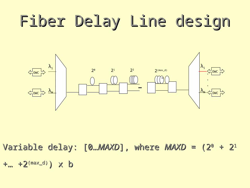
Fiber Delay Line designFiber Delay Line design
Variable delay: [0…Variable delay: [0…MAXDMAXD], where ], where MAXDMAXD = (2 = (200 + 2 + 211 +… +2 +… +2(max_d)(max_d)) x b) x b
λ1
. . .λW
λ1
. . .λW
…
20 21 22
…
2(max_d)OWC
OWC OWC
OWC

Benefits of FDLs and OWCsBenefits of FDLs and OWCsSwitch design benefits with NSFNET Topology
FDLs vs. OWCs in 2-WM DS nodes (W=16)
0
0.05
0.1
0.15
0.2
0.25
0.3
0.1 0.2 0.3 0.4 0.5 0.6 0.7 0.8 0.9 1
Load intensity
Bu
rst
los
s p
rob
ab
ilit
y
No FDLs-No OWCs
OWCs only
FDLS only
FDLs and OWCs
FDLs vs. OWCs with JET signaling and W=16

In a fully connected network (all nodes are connected), OWC has no effect on the blocking performance but FDLs do.
FDLs and OWCs capabilities must be used judiciously and placed in nodes that maximize the performance.
k-LOSS heuristic [JIM99, MSS02]: Via simulation, Place OWC in nodes experiencing the highest blocking rates.
Efficient FDLs/OWCs placementEfficient FDLs/OWCs placement
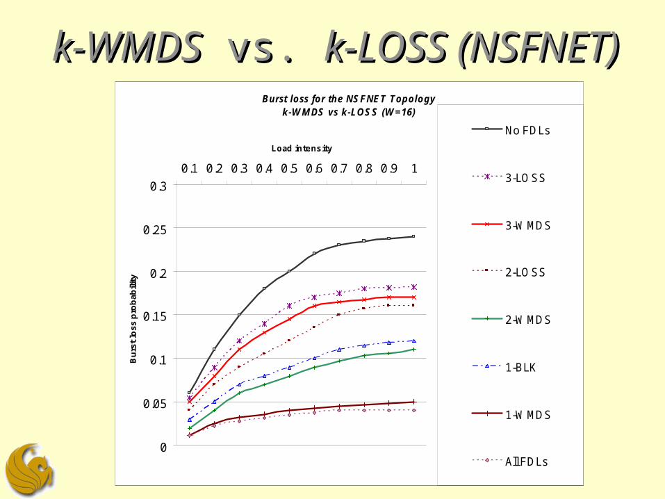
k-WMDSk-WMDS vs. vs. k-LOSS (NSFNET)k-LOSS (NSFNET)Burst loss for the NSFNET Topology
k-WM DS vs k-LOSS (W=16)
0
0.05
0.1
0.15
0.2
0.25
0.3
0.1 0.2 0.3 0.4 0.5 0.6 0.7 0.8 0.9 1
Load intensity
Bu
rst
loss
pro
bab
ility
No FDLs
3-LOSS
3-WMDS
2-LOSS
2-WMDS
1-BLK
1-WMDS
All FDLs
ConclusionConclusion
k-MDS provides an efficient sparse OWC placement.
k-WMDS models non-uniform traffic patterns.
k-MDS allows efficient placement of limited OWC.
It applies to G-nodes selection for traffic grooming.
k-WMDS efficiently place FDLs.

Discussion Discussion
and and
QuestionsQuestions