Architecture-AwareApproximateComputingxzt102.github.io/publications/2019_SIGMETRICS_3_Xulong.pdf ·...

38

Architecture-Aware Approximate Computing

MUSTAFA KARAKOY, TOBB University of Economics and Technology, TURKEY

ORHAN KISLAL, Pennsylvania State University, USAXULONG TANG, Pennsylvania State University, USAMAHMUT TAYLAN KANDEMIR, Pennsylvania State University, USAMEENAKSHI ARUNACHALAM, Intel, USA

Deliberate use of approximate computing has been an active research area recently. Observing that many

application programs from diferent domains can live with less-than-perfect accuracy, existing techniques try

to trade of program output accuracy with performance-energy savings. While these works provide point

solutions, they leave three critical questions regarding approximate computing unanswered, especially in the

context of dropping/skipping costly data accesses: (i) what is the maximum potential of skipping (i.e., not

performing) data accesses under a given inaccuracy bound?; (ii) can we identify the data accesses to drop

randomly, or is being architecture aware (i.e., identifying the costliest data accesses in a given architecture)

critical?; and (iii) do two executions that skip the same number of data accesses always result in the same

output quality (error)? This paper irst provides answers to these questions using ten multithreaded workloads,

and then, motivated by the negative answer to the third question, presents a program slicing-based approach

that identiies the set of data accesses to drop such that (i) the resulting performance/energy beneits are

maximized and (ii) the execution remains within the error (inaccuracy) bound speciied by the user. Our

slicing-based approach irst uses backward slicing and then forward slicing to decide the set of data accesses

to drop. Our experimental evaluations using ten multithreaded workloads show that, when averaged over all

benchmark programs we have, 8.8% performance improvement and 13.7% energy saving are possible when

we set the error bound to 2%, and the corresponding improvements jump to 15% and 25%, respectively, when

the error bound is raised to 4%.

CCS Concepts: · Computer systems organization→ Multicore architectures;

Additional Key Words and Phrases: Approximate computing, compiler, manycore system

ACM Reference Format:

℧ustafa Karakoy, Orhan Kislal, Xulong Tang, ℧ahmut Taylan Kandemir, and ℧eenakshi Arunachalam. 2019.

Architecture-Aware Approximate Computing. Proc. ACM Meas. Anal. Comput. Syst. 3, 2, Article 38 (June 2019),

24 pages. https://doi.org/10.1145/3326153

1 INTRODUCTION

Constraints imposed by hardware scaling and data and control dependencies across computationscombined by compilers' inability to maximize computation parallelism limit the performancepotential of multithreaded workloads running on emerging manycore systems. State-of-the-art

Authors' addresses: ℧ustafa Karakoy, TOBB University of Economics and Technology, Ankara, TURKEY, m.karakoy@yahoo.

co.uk; Orhan Kislal, Pennsylvania State University, State College, PA, 16801, USA, [email protected]; Xulong Tang,

Pennsylvania State University, State College, PA, 16801, USA, [email protected]; ℧ahmut Taylan Kandemir, Pennsylvania

State University, State College, PA, 16801, USA, [email protected]; ℧eenakshi Arunachalam, Intel, Hillsboro, Oregon, 97124,

USA, [email protected].

Permission to make digital or hard copies of all or part of this work for personal or classroom use is granted without fee

provided that copies are not made or distributed for proit or commercial advantage and that copies bear this notice and

the full citation on the irst page. Copyrights for components of this work owned by others than AC℧ must be honored.

Abstracting with credit is permitted. To copy otherwise, or republish, to post on servers or to redistribute to lists, requires

prior speciic permission and/or a fee. Request permissions from [email protected].

© 2019 Association for Computing ℧achinery.

2476-1249/2019/6-ART38 $15.00

https://doi.org/10.1145/3326153

Proc. AC℧ ℧eas. Anal. Comput. Syst., Vol. 3, No. 2, Article 38. Publication date: June 2019.

https://doi.org/10.1145/3326153

https://doi.org/10.1145/3326153

38:2 M.Karakoy et al.

research on computer architecture [14, 28, 29, 37], optimizing/parallelizing compilers [6, 17, 44,45, 47] and runtime systems/OS [34, 35, 46] helps us extract increasingly more performance frommodern architectures, but their impact is hampered by ever-growing application and hardwarecomplexities. In particular, data accesses in modern architectures pose a signiicant bottleneck (fromboth performance and energy consumption angles) as they go through multiple layers in hardware,each with its own management strategy. Indeed, there is a growing concern that łmemory wallž[55] can be the main factor preventing many important applications from achieving their fullpotential, even if we employ sophisticated code parallelization and data optimization techniques.Thus, there is a motivation for exploring revolutionary approaches instead of evolutionary ones.

℧any workloads in diferent application domains can live with a łless-than-perfectž outputquality. The application programmers are usually provided with metrics to evaluate the outputquality of a particular application. For instance, in video encoding/decoding applications, PeakSignal to Noise Ratio (PSNR) is a metric that is widely used to measure the quality of lossy videocompression. In this paper, we target the application domains where the programmers have thecapability to determine the error bound of application outputs. Observing this, performance andenergy beneits that arise from deliberate use of so-called łapproximate computingž has recentlybeen explored across software and hardware stacks [1, 8, 11, 15, 24, 38, 42, 50]. Approximatecomputing can be a promising solution in overcoming the inherent performance and energyscalability issues faced by current parallel hardware and software systems due to data accesses. Forexample, skipping some computations can save both computation cycles/energy and cache/memorycycles/energy, which could not be achieved by employing conventional code/data restructuringor hardware enhancements alone. In fact, dropping computations/data accesses can be one of theways to take the performance/energy scalability of parallel workloads to levels that are not possiblethrough evolutionary approaches.

While prior art [34, 36, 51] in approximate computing focused on point solutions that typicallytrade of accuracy (output quality) with performance and energy beneits, existing works do nottarget evaluating the maximum potential of approximate computing or proposing practical schemesthat can come close to this potential. In particular, we believe that the prior research leaves threecritical questions regarding approximate computing unanswered, especially in the context ofdropping/skipping costly data (cache/memory) accesses in data intensive applications:

•What is the maximum potential of skipping (i.e., not performing) data accesses under a giveninaccuracy (output quality) bound?• Can we simply identify the data accesses to drop randomly, or is being architecture aware (i.e.,identifying the łcostliestž data accesses with respect to a given architecture) critical?•Do two executions that skip the same number of data accesses always result in the same outputquality (error)?

℧otivated by these questions, we make two main contributions in this work:

• First, we explore the potential beneits of a form of approximate computing that drops selectdata accesses during the execution of parallel workloads on emerging network-on-chip (NoC)based manycore systems. The unique aspect of this evaluation is its łarchitecture awarenessž.That is, given a bound on inaccuracy (the minimum level of program output quality that can betolerated by user/execution environment), we quantify the beneits of dropping the łcostliestž dataaccesses (in our manycore architecture), as opposed to dropping data accesses łrandomlyž. Ourexperiments with ten diferent multithreaded workloads indicate that being architecture awarein dropping data accesses pays of, resulting in 27% additional performance improvement, overrandomly dropping the same number of data accesses. Unfortunately, our results also indicatethat two diferent executions of a given application that drop the same number of data accesses


Architecture-Aware Approximate Computing 38:3

can result in quite diferent output quality values (errors), which makes it diicult to maximizeperformance under a given error bound.• Second, motivated by this last observation above, we propose a łprogram slicingž based approachthat identiies the set of data accesses to drop such that we (i) maximize the resulting perfor-mance/energy beneits and (ii) remain within the error (inaccuracy) bound speciied by the user.Our slicing based approach irst uses backward slicing and then forward slicing to decide theset of data accesses to drop. Our experimental evaluations of this slicing-based approach undermultithreaded workloads and a cycle-accurate manycore simulator show that, when averagedover all ten benchmark programs we have, 8.8% performance improvement and 13.7% energysaving are possible when we set the error bound to 2%, and the corresponding improvementsjump to 15% and 25%, respectively, when the error bound is set to 4%. We also tested a restrictedversion of our approach on a commercial manycore system, and observed 6.8% and 11.2% averageperformance improvements with error bounds of 2% and 4%, respectively.

The remainder of this paper is structured as follows. The next section presents our targetmanycore architecture, and discusses diferent types of potential łdata localitiesž in this architecture.Section 3 explains the idea of łdropping data accessesž at a high level, and Section 4 presents ourexperimental setup and benchmark programs. Section 5 gives a quantitative analysis of the outputqualityś performance/energy saving tradeof by varying the number and locality category of thedata accesses to be dropped. Section 6 discusses our program slicing-based approach to approximatecomputing, and provides experimental evidence that shows its efectiveness in practice. Section 7discusses the related work, and inally, Section 8 concludes the paper.

2 TARGET MANYCORE ARCHITECTURE, DATA ACCESS, AND DIFFERENT

LOCALITIES

MC MC

MC MC

L1

L2 Router!

Core

L1

L2 Bank

Fig. 1. Representation of a 4 × 8 NoC system with and SNUCA based memory access flow.

Since one of the goals of this work is to measure the limits of architecture-aware approximatecomputing, we need to explain the łcost of a data accessž from an architecture viewpoint. Figure 1shows the architecture of a state-of-the-art network-on-chip (NoC) based manycore system (similarto Intel KNL [40] and many emerging commercial manycore systems) and the low of a data accessin it under the SNUCA last-level cache (LLC) management policy1. First, the local L1 cache islooked up ( 1 ), and if a miss occurs, an L2 bank (which is determined based on the physical addressof the data being requested) is accessed ( 2 ). If we hit in the target L2 bank, the data is read andtransferred to the local L1 of the requesting core ( 6 ). If not, an of-chip memory access needsto be performed. For this, irst, a target memory controller (℧C) is determined (again, based onthe physical address of the data being requested) and we access the target bank governed by that

1In SNUCA [13], each data block is statically mapped to an L2 cache bank (called its łhome bankž) based on its physical

address. A core/node that requires a speciic data item brings it from its home bank if it is in the cache. If not, the main

memory is accessed, again using the physical address of the data. Note that although our target system has two levels of

cache hierarchy (L2 being the last-level cache), our approach can work with cache hierarchies of any depth.



MC MC

MC MC

L1

L2

(a) L2 hit (SQ).

MC MC

MC MC

L2

(b) row-bufer hit/miss(SQ).

MC MC

MC MC

L1

L2

(c) L2 hit (DQ).

MC MC

MC MC

L2

(d) row-bufer hit/miss(DQ).

Fig. 2. Various data localities in an on-chip network based manycore. Note that the diference between arow-bufer hit and a row-bufer miss manifests itself in the of-chip memory.

controller via the on-chip network ( 3 ). Each bank is equipped with a row-bufer that holds themost recently accessed memory row (also called page); typically, a row-bufer hit takes much lesstime than a row-bufer miss, as the latter requires an access to the memory array itself. After thedata is read ( 4 ), it is returned to L2 ( 5 ), the home bank for the requested data, and then to L1 ( 6 ).In this architecture, at a high level, one can distinguish among at least four diferent types of

data localities, depending on where the data being sought is found: L1 hit, L2 hit, row-bufer hit,and row-bufer miss. The actual latency numbers for these diferent localities may change fromone architecture to another. ℧ore interestingly, the latency to be incurred in the last three casesmay not be uniform, as the distance to target L2 bank and target ℧C may vary (on the network),depending on the relative locations of the requesting node/core and target L2 bank/℧C. Therefore,not all L2 accesses (and similarly not all ℧C accesses) have the same latency, and consequently,one can have a spectrum of L2 and ℧C latencies from a given core's perspective. For the purposesof this work however, we consider seven diferent types of localities: L1 hit, L2 hit (SQ), L2 hit (DQ),row-bufer hit (SQ), row-bufer hit (DQ), row-bufer miss (SQ), and row-bufer miss (DQ). In thisnaming, SQ denotes the łsame quadrantž, i.e., when the requesting core and the target L2 are inthe same quadrant of the network (in the case of an L2 hit) and when the requesting L2 and thetarget ℧C are in the same quadrant (in the case of an L2 miss). DQ on the other hand capturesthe case when the core (resp. L2) and target L2 (resp. ℧C) are in diferent quadrants. These casesare captured in Figure 2. In the rest of this paper, for brevity, these seven types of data localities(also called łcategoriesž, or łgroupsž in this work) are denoted using C1 (for L1 hit), C2, C3, C4, C5,C6, and C7 (for row-bufer miss (DQ)). Clearly, everything else being equal, for a given data accessin our manycore architecture, we would prefer to have Ci instead of Ci+1 (1 ≤ i ≤ 6) from a datalocality viewpoint. In fact, many previously-published software and hardware works targeting”data locality” (in the context of both single-core and manycore systems), try to move as many dataaccesses as possible, from Cj to Ci where 1 ≤ i < j ≤ 7.

3 DROPPING DATA ACCESSES

While there exist diferent approaches [11] to approximate computing, each leading to a diferenttradeof between performance/energy beneits and program output accuracy, in this work we usełskipping/dropping data accessesž. Three other possible approaches are (i) dropping computations,(ii) dropping synchronizations, and (iii) reducing the number of bits used to implement individualdata elements. In loop perforation [39], computations (some loop iterations) are dropped in a system-atic fashion. While this computation skipping technique is quite efective in some applications, ingeneral dropping an iteration means dropping a considerable number of data accesses (especially inthe case of large loop bodies) along with the computations that operate on them, and consequently,its impact on the accuracy of the application can be very signiicant. As a result, one may prefer toemploy a iner granular technique, e.g., data access skipping that is used in this work. An alternate



approach to approximate computing is to reduce the number of synchronizations in the applicationcode. ℧any high-performance computing applications are implemented in a multithreaded fashionand execute using a very large number of threads (sometimes tens of thousands). In such cases,a barrier synchronization (which is meant to synchronize all threads) can be very costly latencywise. In [32], the barrier is opened right after a certain fraction of threads reach it, instead ofwaiting for all threads to reach it. One problem with this approach is that it may not be veryefective in applications where there are not lots of synchronizations. Even in applications withlots of synchronizations, it is hard to predict the impact of relaxing barriers on program accuracy.The third alternate technique, reducing the number of bits to represent values of individual dataelements [33], while can be efective in certain application domains, may not be the best it for otherapplications that need full bit width. ℧otivated by these observations, in this work, we use ”dataaccess skipping”, which is iner grain than heavy-handed computation skipping, and is applicableto programs with loating point (as well as integer) data and those with no/few synchronizations.We want to emphasize that, while dropping data accesses can lead to program crash in certain

cases, this is not expected to be the case in our target application domain. Basically, in this work,we focus on array and loop dominated programs from high performance computing and embeddedimage/video processing. These codes are generally written as a series of loop nests, and each nesthaving a large body of instructions. The speciic execution path taken by the program is mostly afunction of the input size but is not dependent on the actual values of the inputs. Thus, changes inthe values of the data elements (which is an efect of our approach, as we supply a łvaluež for eachdata access we drop) does not cause an otherwise correct program to crash.The goal behind data access dropping/skipping is to drop the right number of data accesses

to maximize the performance/energy beneits and at the same time remain within the limits ofłacceptable output inaccuracyž (output quality). Clearly, the latter is a function of the applica-tion/workload characteristics and can sometimes even change from one execution environment(e.g., user constraints, input) to another, for the same application program. This paper is based on asimple yet important observation:

If we are allowed to drop a certain amount of data accesses so that the program’s outputquality is still acceptable, to maximize performance/energy beneits, we may want to dropthe łcostliestž data accesses irst.

Considering our classiication of data locality in Section 2, we want to irst drop the accessesin the C7 category; if we can continue to drop more data accesses (and still remain within theuser-speciied error bound), they should be picked from the C6 category; and so on. That is, theobservation above tells us that, in dropping data accesses, we should be łcost/architecture awarež.However, there is no guarantee that, two executions that drop the same number of references withexactly the same cost would result in the same inaccuracy. In other words, just adopting, as ourquality metric, the number of the data accesses to be dropped or their associated costs may notguarantee that the resulting output accuracy of the application program would be acceptable froma user's perspective. This is because the inaccuracy resulting from dropping data accesses is notonly a function of the number of data accesses dropped but also a function of which speciic dataaccesses are dropped.℧otivated by this observation, the rest of the paper makes two major contributions. First, we

perform a quantitative analysis of the tradeof between performance/energy beneits and inaccuracy(QoS) under varying amounts of data access skipping. The goal of this analysis is to demonstratethe importance of dropping the costliest data accesses (as opposed to, say, łrandomlyž selectingthe data accesses to drop). We also investigate the variation in the program output qualities oftwo diferent executions of the same program, when in both the executions the same number of



Table 1. Target system configuration.

℧anycore Size, Frequency 32 (4 × 8), 1 GHzL1 Cache 16 KB; 8-way;

32 bytes/lineL2 Cache 512 KB/core; 16-way;

64 bytes/lineCoherence Protocol ℧OESIRouter Overhead 3 cyclesPage Size 2 KBOn-Chip Network Frequency 1 GHzRouting Strategy XY-routingDRA℧ DDR3-1333 (9-9-9);

250 request bufer entries;4 ℧Cs 1 rank/channel;16 banks/rank

Row-Bufer Size 2 KBAddress Distribution across LLCs 64 bytesAddress Distribution across banks 64 bytesEpoch Length 256 cycles

0

20

40

60

80

100

Bre

akd

ow

n o

f D

ata

Lo

cality

(%

)

C1 C2 C3 C4 C5 C6 C7

Fig. 3. Data locality breakdown of our multithreaded application programs.

(but diferent) data accesses are dropped. Our results show that this variation can be quite high.℧otivated by this, we then propose a łprogram slicingž based strategy that drops the right set ofdata accesses to guarantee the inaccuracy bound speciied by the user/programmer. Unless statedotherwise, when we say ła data access is droppedž, we mean that the corresponding access is notperformed and instead a value of ł0ž is assumed for that access. Later, we discuss an alternate strategy(based on application proiling) to supply the missing values.2

4 BENCHMARKS AND EXPERIMENTAL SETUP

The program slicing technique (and the required code analysis) used in this work is implementedwithin the LLV℧ framework [19]. ℧ost of our experiments are conducted using a cycle-accuratemanycore simulator. ℧ore speciically, in our experiments, we use the GE℧5+℧cPAT [3, 20]combination to collect performance and energy statistics. Note that the reported energy numbersinclude the energy consumed by all CPU components, caches, TLBs as well as main memory. Theimportant parameters of the modeled on-chip network based manycore system along with theirdefault values are listed in Table 1. Later in our experiments we modify the values of some of theseparameters to conduct various sensitivity experiments. We preferred a simulator-based analysis, asit is diicult in current architectures to be able to drop data accesses at a ine granularity (dynamicinstance based) and it is also diicult to isolate the performance of data accesses. Nevertheless, wealso tested a restricted version of our approach on a state-of-the-art manycore architecture [40],and report the collected results in Section 6.5.

2We want to emphasize that only the mentioned alternative strategy uses ”proiling”; our original approach that supplies ł0ž

for the dropped accesses does not need proiling.



Table 2. Our multithreaded workloads and their salient characteristics.

Benchmark Source Error (Quality) Input DatasetMetric Size (MB)

LU Splash-2 [54] Relative diference 565.8from standard output

Sparse℧at local Relative diference 521.2Vect℧ult from standard outputSwaptions Parsec [2] Relative diference 487.5

from standard outputBarnes-Hut Splash-2 [54] Relative diference 663.3

from standard outputx264 Parsec [2] PSNR 702.6ImgSmooth local PSNR 712.4Raytracer Splash-2 [54] Pixel Diference 762.5VolRend Splash-2 [54] Pixel Diference 522.9Ferret Parsec [2] Classiication accuracy 698.7SSI local Ranking accuracy 608.7

In this study, we used 10 multithreaded benchmark programs3. In our experiments, only onemultithreaded application is executed at a time (using all 32 cores). The second column in Table 2gives the sources of our benchmark programs and the third column gives the error (output quality)metric used for each benchmark. In this column, łRelative Diferencež is the root-mean-squareerror of the output. Note that, the same error metrics have also been used by prior research onapproximate computing [7]. For x264 and ImagSmooth, we used Peak Signal to Noise Ratio (PSNR)as error metric to measure the quality of output images. For Ferret, we used classiication accuracy(calculated by the average of similarity diferences). It can be observed from this column that ourworkloads employ a variety of error (quality) metrics. Finally, the last column of this table gives thetotal amount of input dataset in ℧Bs. We start by presenting the breakdown of data accesses foreach benchmark program we have into the seven locality categories (C1 · · ·C7) explained earlierin Section 2. The results plotted in Figure 3 indicate that our applications exhibit great variety interms of the data locality they exhibit. For example, locality behaviors of ImgSmooth and SSI arequite well, with very few data accesses fall in the C4 −C7 range. In comparison, applications suchas Barnes-Hut and x264 exhibit poor data locality, with nearly most of their data accesses falling inthe C4 −C7 range.

5 EVALUATION OF THE PERFORMANCE/ENERGY BENEFITS AND OUTPUT

INACCURACY TRADEOFF

In this section, we evaluate our benchmark programs in terms of four diferent metrics whilevarying the fraction of data accesses to be dropped: memory access latency improvement, overallperformance improvement, energy savings, and output error (inaccuracy). All these metrics are givenas relative (percentage) values with respect to the default execution where łnož data access isdropped (in this default case, the program output quality is assumed to be perfect). Recall that thethird column of Table 2 gives the error (quality) metric for each benchmark. In the x axes of thegraphs presented below, ł5% of C7ž refers to an execution where 5% of the data accesses in theC7 category (as deined in Section 2) are dropped. Similarly, ł100% of C7 + 5% of C6ž captures anexecution where all of the C7 type of data accesses as well as 5% of the C6 type of data accesses aredropped, and so on. Note that the percentage performance (energy) improvement values representthe percentage reduction/saving over the execution time (energy consumption) of the defaultexecution. Also, each result presented below in Figures 4, 5, 6, and 7 represents the łmedian valuesžcollected from 20 diferent executions. Finally, in an execution where we are to drop a certain

3These benchmarks have been fully optimized for parallelism and data locality using O3 compiler lag.



0

20

40

60

80

100

Imp

rove

me

nt

in D

ata

A

cc

ess

La

ten

cy (

%)

5% of C7 10% of C725% of C7 50% of C7100% of C7 100% of C7 + 5% of C6100% of C7 + 10% of C6 100% of C7 + 25% of C6100% of C7 + 50% of C6 100% of C7 + 100% of C6100% of C7 + 100% of C6 + 100% of C5 100% of C7 + 100% of C6 + 100% of C5 + 100% of C4

Fig. 4. Improvements in data access latencies.

0

20

40

60

80

100

Perf

orm

an

ce

Im

pro

ve

me

nt

(%)

Fig. 5. Performance improvements. The legend is the same as in Figure 4.

0

20

40

60

80

100

En

erg

y S

avin

gs (

%)

Fig. 6. Energy savings. The legend is the same as in Figure 4.

0

20

40

60

80

100

Pe

rfo

rma

nc

e I

mp

rov

em

en

t (%

)

Rnd1 Rnd2 Rnd3 Rnd4 Rnd5 Rnd6 Rnd7 Rnd8 Rnd9 Rnd10 Rnd11 Rnd12

Fig. 7. Performance improvements.

fraction of data accesses, those accesses are determined randomly. For example, if, say, we aredropping 10% of theC7 type of data accesses, that 10% accesses are selected randomly (from amongall C7 type of accesses).

In the discussion below, we try to answer three important questions: (i) how much performanceand energy can one save by dropping the łcostliestž memory accesses?; (ii) how do these beneits compareto an alternate strategy that simply drops the data accesses łrandomlyž, i.e., without considering which



locality category they belong to?; and (iii) is the magnitude of performance and energy savings obtainedvia data access skipping a function of only the amount of the data accesses to drop, or also of the dataaccesses themselves?The graph in Figure 4 gives the percentage improvement in the average łdata access latencyž

under diferent execution scenarios (the x-axis represents the fraction and category of the dataaccesses dropped). As expected, data access latencies drop, as we increase the number of dataaccesses to drop. However, improvement trends vary across diferent workloads. For example, SSIdoes not exhibit signiicant improvements except in the last two executions. In contrast, LU andVolRend show reasonable improvements in memory access latencies, even when the number of dataaccesses dropped is not too high. While data access latency is certainly an important metric, onewould ultimately be interested in overall application performance, which is plotted in Figure 5. Thisgraph gives the percentage reduction in the parallel execution time (over the default execution).Clearly, diferent applications get diferent beneits due to the diferent contributions of the memoryaccesses in them to their overall performance. Still, one can observe a common pattern where theperformance beneits are initially not very high but they show a signiicant jump beyond a certainpoint. For example, in VolRend, the performance beneits jump signiicantly as we move from ł50%of C7ž to ł100% of C7ž. A similar jump can be observed in x264 and Barnes-Hut as well.Figure 6 plots the energy beneits (given as percentage reduction in system-wide energy con-

sumption over the default execution) when dropping various number of data accesses (as speciiedon the x-axis). We see that these results are in general higher than the performance improvementresults presented in Figure 5. This is primarily because, in the default execution, a costly data accesscan overlap with other (ongoing) data accesses or computations. Consequently, dropping such anaccess may not return much beneits in practice. In contrast, while performance overhead of a dataaccess can be hidden in parallel execution, its energy overhead cannot be; and, as a result, droppinga data access gives more energy beneits than performance beneits, when compared to the defaultexecution. Overall, the results presented in Figures 5 and 6 clearly indicate that dropping costlymemory accesses can give signiicant performance and energy beneits.Let us now try to answer the second question raised above, namely, whether dropping the

costliest accesses (as opposed to other accesses) is really important, as far as the performance andenergy beneits are concerned. Figures 7 and 8 give, respectively, the performance and energybeneits (again with respect to the default execution), when we select the data accesses to droprandomly from all data accesses4. In these two charts, each point on the x-axis corresponds to anexecution that drops the łsame numberž of data accesses as the corresponding point in Figures 5and 6. For example, łRnd2ž in Figure 7 drops the same number of data accesses as ł10% of C7ž inFigure 5, and łRnd11ž drops the same number of data accesses as ł100% of C7 + 100% of C6ž inFigure 5. Comparing the results in Figures 7 and 8 with the corresponding results in Figures 5 and 6clearly indicates that one needs to be very careful in selecting the data accesses to drop, as can also beseen from the geometric mean results plotted in Figures 9 and 10. For example, the execution withł10% of C7ž drops generates about 27% additional performance improvement and 31% additionalenergy improvement compared to randomly dropping the same number of data accesses.We next focus on output quality of our application programs and quantify it when dropping

various number of costly data accesses. There can be diferent metrics to quantify the outputquality of an application, and in general two applications may have diferent metrics to quantifytheir output qualities. As stated earlier, in this work, we used the metrics listed under the third

4It is to be noted that, in the earlier case (Figures 5 and 6) where we dropped the costliest references, we use random

selection only from a given category. For example, when we talked about dropping 10% of the C7 category of data accesses,

that 10% is selected randomly (but only from the C7 category). In contrast, here, the data accesses to be dropped are selected

randomly from all data accesses.



0

20

40

60

80

100

En

erg

y S

av

ing

s (

%)


Fig. 8. Energy savings.

01020304050

Rnd1 Rnd2 Rnd3 Rnd4 Rnd5 Rnd6 Rnd7 Rnd8 Rnd9 Rnd10 Rnd11 Rnd12Pe

rfo

rma

nc

e

Imp

rove

me

nt

(%)

Architecture Aware Random

Fig. 9. Geometric mean of performance improvements across all applications. Note that, each point on thex-axis represent diferent entities for locality aware and random schemes. In the later, it represents randomselections of the data accesses to be dropped. In the former, it represents the corresponding point in Figure 5.

0

20

40

60

80


En

erg

y S

avin

gs

(%

)

Architecture Aware Random

Fig. 10. Geometric mean of energy savings across all applications. Note that, each point on the x-axis representdiferent entities for locality aware and random schemes. In the later, it represents random selections of thedata accesses to be dropped. In the former, it represents the corresponding point in Figure 6.

0

20

40

60

80

100

Err

or

(%)

5% of C7 10% of C725% of C7 50% of C7100% of C7 100% of C7 + 5% of C6100% of C7 + 10% of C6 100% of C7 + 25% of C6100% of C7 + 50% of C6 100% of C7 + 100% of C6100% of C7 + 100% of C6 + 100% of C5 100% of C7 + 100% of C6 + 100% of C5 + 100% of C4

Fig. 11. Error (program output inaccuracy) values.

column of Table 2. The y-axis in Figure 11 represents the percentage error experienced over thedefault execution (reduction in output quality). As in the case of performance behavior, in mostbenchmarks, the error jumps signiicantly beyond a point (which depends on the benchmark). Forinstance, in Ferret, the error moves from 8% to 28%, as we move from ł100% of C7 + 50% of C6ž toł100% of C7 + 100% of C6ž.

We now turn our attention to the third question raised above.When considering both performanceimprovements (Figure 5) and corresponding errors (Figure 11), one might think that, it could bepossible to decide the łideal number of data accessesž to skip in order to save as much performanceand energy as possible while staying within an acceptable error bound. As an example, in Swaptions,



Table 3. Distribution of output errors in LU.

5% 10% 25% 50% 100%100% of C7100% of C7100% of C7100% of C7 100% of C7 100% of C7+100% 100% of C7+100% of C6of C7of C7of C7of C7of C7 +5% of C6 +10% of C6+25% of C6+50% of C6+100% of C6of C6+100% of C5+100% of C5+100% of C4

minimum 0.02 0.06 0.09 0.14 0.2 1.13 2.26 3.87 8.28 19.68 28.06 89.2median 0.05 0.09 0.15 0.25 0.33 2.33 4.84 8.16 15.27 28 44.4 92.3maximum 1.9 3.34 5.87 8.11 11.14 14.72 16.67 18 24.45 41 62.22 98

Table 4. Distribution of output errors in VolRend.

5% 10% 25% 50% 100%100% of C7100% of C7100% of C7100% of C7 100% of C7 100% of C7+100% 100% of C7+100% of C6of C7of C7of C7of C7of C7 +5% of C6 +10% of C6+25% of C6+50% of C6+100% of C6of C6+100% of C5+100% of C5+100% of C4

minimum 0.13 0.25 0.77 4.31 12.05 18.27 28.45 45.04 56.12 68.56 78.16 94.02median 0.23 0.54 1.34 8.13 17.41 28.01 41.4 59 71.11 85.05 91 98.34maximum 2.22 3.16 4.49 12.68 24.24 37.78 53.7 72.67 84.21 96.16 97.71 99.12

if the maximum error that can be łtoleratedž is 10%, we can see that ł100% of C7ž is the right amountto drop, and this leads to about 46.7% improvement in overall application performance. A similaranalysis can be carried out for any application program and any given error bound. However, inpractice, this approach may not be easy to implement. This is because, as indicated earlier, theresults presented in Figure 6 represent the łmedian valuesž from 20 diferent executions. Table 3and Table 4 give the łdistributionž of the errors from our 20 diferent experiments for LU andVolRend, respectively. The error results are given in these tables as minimum, median and averageerror values. One important observation from these results is that, there are łsigniicant variationsžacross error values. To be more speciic, two diferent executions of an application that drop thesame number of data accesses from the same set of categories (localities) can lead to signiicantlydiferent errors in the output of an application. Consequently, it may not be possible to simply lookat the performance and error plots, and determine the right amount/type of data access(es) to drop.Furthermore, this result also means that, it is not trivial to put a bound on error when a certainnumber of data accesses are dropped. ℧otivated by these observations, the next section proposesand experimentally evaluates a łprogram slicingž based strategy to determine the data accesses todrop such that (i) performance beneits are maximized and (ii) we remain within a user-speciied errorbound.

6 PROGRAM SLICING-BASED DATA ACCESS REMOVAL

We now discuss our program slicing-based approach employed to decide the set of variables to dropsuch that the performance is maximized and the accuracy loss is within a speciied error bound.At a high level, our approach computes, using backward and forward slicing (explained below) aswell as target error metric, the performance gains when accuracy of output elements are relaxed.Among all possible relaxations, our approach then selects the one that generates the maximumperformance beneits while staying within the speciied error bound.

6.1 Program Slicing Basics

Program slicing is a source code analysis strategy that identiies code segments relevant to a givenprogram point in the target code base. The initial idea was proposed by Weiser for the purpose ofsimplifying debugging [53]. Slicing is also used in program diferencing, optimization, maintenance,and lowback analysis [48]. While the original concept ensures that a code slice is a syntacticallyvalid program, more recent algorithms relax this constraint to provide more accurate (smaller)slices. There are two main forms of program slicing. Static slicing, which is the one employed inthis work, uses only statically measurable information and it is applicable for any execution of the



05

10152025303540

Perf

orm

an

ce Im

pro

vem

en

t (%

)

error ≤ 1%

Random Slicing Based

05

1015202530354045

Perf

orm

an

ce Im

pro

vem

en

t (%

)

error ≤ 2%


05

1015202530354045

Perf

orm

an

ce Im

pro

vem

en

t (%

)

error ≤ 4%


05

1015202530354045

Pe

rfo

rma

nc

e Im

pro

ve

me

nt

(%)

error ≤ 6%


05

1015202530354045

Perf

orm

an

ce Im

pro

vem

en

t (%

)error ≤ 8%


0

10

20

30

40

50

60

Perf

orm

an

ce Im

pro

vem

en

t (%

)

error ≤ 10%


Fig. 12. Performance improvements.

program. On the other hand, dynamic slicing is tailored to a particular execution of the programwhich requires a ixed set of input values [18].

To explain how a code slice is obtained, it is important to deine the following dependencyconcepts. Let P1 and P2 be two program points. P2 has a ”data dependency” on P1 if there existsa variable v that satisies all of the following conditions: (i) P1 modiies the value of v; (ii) P2reads the value of v; and (iii) There is an execution path from P1 to P2 on which the value of vis not overwritten. Note that, slicing captures ”indirect dependencies” as well. For instance, incode sequence {S1 : u = v + 1; S2 : w = u − b; S3 : t = w ∗ w − 1; }, the indirect dependencebetween statement S1 and statement S3 is also captured (in addition to two direct dependencies,one between S1 and S2, and the other between S2 and S3). On the other hand, P2 is said to have a”control dependency” on P1 if at least one of the following conditions is true: (i) P1 is a conditionstatement, and reaching P2 depends on P1; (ii) P1 is a function call, and P2 is one of the parametersof the call; (iii) P1 is a function call, and P2 is the entry point of a function called by P1; and (iv) P1is a function entry point, and P2 is one of the formal parameters, one of the declarations, or one ofthe top-level statements in the body of the function.A program slice can be expressed as a set of data and control dependencies. There are two

”directions” a program slice can be extracted since a dependency requires two actors. BackwardSlice of a given point is the union of the points it depends on. Similarly, Forward Slice of a point isthe union of its dependent points. Since both of these are calculated are using the same dependencyrelations, our explanation below mostly focuses on backward slicing.

Figure 13(a) shows a sample code fragment, and Figure 13(b) shows a static backwards slice fromline 14, variable x (denoted as < 14,x >). < 14,x > has a data dependency on lines 6 and 8 as theymodify the value of x . These two lines are controlled by the if statement (lines 5 and 7) and thewhole block is controlled by the while statement (lines 4 and 13). Finally, the while condition isdata dependent on lines 1, 3, and 12. The remaining lines (2, 9, 10, 15, and 16) are safely omittedfrom the slice. A dynamic backward slice from the same point may or may not be the same as itsstatic counterpart. Assuming the value of n is 1; line 8 will not be included in the slice, since thecontrol never reaches that point in the irst place.



1. read(n);

2. read(m);

3. i = 0

4. while i < n do

5. if i mod 2 = 0 then

6. x = 1;

7. else

8. x = 2;

9. y = y + m;

10. read(m);

11. end if

12. i = i +1

13. end while

14. print(x)

15. print(y)

16. print(&x)

1. read(n);

2.

3. i = 0

4. while i < n do

5. if i mod 2 = 0 then

6. x = 1;

7. else

8. x = 2;

9.

10.

11. end if

12. i = i +1

13. end while

14. print(x)

15.

16.

(a) (b)

1. int x(n), y(n), t(n);

2. int k;

3. k = … 4. x(1) = …5. x(2) = …6. x(3) = …7. y(1) = …8. y(2) = …9. y(3) = …10. t(1) = … 11. t(2) = …12. t(3) = …13. … = …14. … = (x(1) + x(2)) / k; 15. … = … 16. z(1) = (x(1) + y(1) + t(1)) * k;

17. z(2) = (x(2) + y(2) + t(2)) * k;

18. z(3) = (x(3) + y(3) + t(3)) * k;

(c)

Fig. 13. (a) An example code fragment to illustrate program slicing. (b) Static backward slice from Figure 13afor line 14, variable x . (c) An example code segment.

Note that a backward slice may contain lines after that particular point (and vice versa for forwardslice). For example, a backward slice from < 9,m > will include line 10, as its result does efectline 9 in a diferent iteration of the while loop. In addition, it is important to note the distinctionbetween values and their addresses. As an example, < 16,&x > does not depend on lines 6 or 8 (orany other line) since the actual address of the variable does not change and the value is irrelevantfor this particular point in the program.

The calculation of a forward slice follows the data and control dependency chains in the reversedirection. For example, static forward slice of < 2,m > contains lines 9 and 15. Line 9 dependson the value ofm and, even thoughm it is overwritten at line 10, this dependency propagates toline 15 through the value of y. Forward slicing is a useful method to classify points based on theirpotential impact on the rest of the program. This classiication may lead to various optimizations,e.g, which variable should have less precision?, which calculation should be approximated?, etc.Program slicing has been extended to handle iteration spaces and multi-dimensional arrays by

Pugh and Rosser [30]. In our work, we closely follow their implementation of program slicing.Speciically, we generate, without completely unrolling the loop nests, an iteration space slice, if theloop bounds and array subscript expressions are aine functions of outer loop bounds and symbolicconstants. In more detail, the backward iteration space slicing takes, as input, the dependencyinformation (extracted by the compiler) and determines all statement instances (in loops) that needto be executed to produce the values of a given array access. Consequently, a slice obtained in thisway can be thought of as a łdependence chainž that can be used to reach all statement instanceswhich can afect the result. In the next section, we give the technical details of our slicing-basedcompiler algorithm.

6.2 Slicing for Approximate Computing

Algorithm 1 gives the pseudo-code of our slicing-based compiler algorithm. The complexity of thealgorithm is O(NM2) where N is the number of outputs andM is the number of statements involvedin backward slicing and forward slicing. At a high level, our algorithm irst extracts a backwardslice for each element of the output data structure (line 36). After that, for each left-hand-sidevariable involved in any statement in the backward slice, it determines the forward slice (line 37).If that forward slice includes any other statement other than the one we started the backwardslice from, we mark that variable as łnon-approximatablež. The remaining variables on the otherhand (i.e., the variables that can be approximated/skipped if we accept error in the output elementin question) constitute the łapproximation setž of that output data element (line 38). Then, foreach data element (access) in this set, we estimate its cost in terms of the number of cycles it



is expected to take in the target architecture (using the Cost_Evaluation function) (line 56), andsubsequently ind the total number of cycles that can potentially be saved if we accept error in thatoutput element. This process is then repeated for each output element, and after all the outputelements have been processed, we have the łapproximation setž of each output data element. Inthe next step, we go over all variables in łapproximation setž and identify the k most beneicialoutput data elements (accesses) to drop, where k is determined by the total number of output dataelements and the acceptable error value speciied by the user (err). We want to emphasize that ourapproach guarantees that the user-speciied error bound is satisied, i.e., among all options, we pickk elements (to drop) that satisfy the error bound and generate maximum savings. Therefore, ourprogram slicing based approach is also łcost (architecture) awarež in that it drops that data accessesthat return the most beneits. Note also that, since we carry out our compiler analysis at a dataelement granularity (actually, if desired, its granularity can be tuned), we catch the opportunities fordropping data accesses even if the same data element is accessed by diferent static load instructionsin the code.

In this work, we implemented theCost_Evaluation function by extending a cache miss estimationscheme called C℧E (cache miss equations [9]). C℧E is originally designed to give a detailedrepresentation of cache behavior, including conlict misses, in loop-oriented application programs.5

We extended the original C℧E implementation to capture coherence misses (in multithreadedexecution), misses in cache hierarchies of any depth, as well as row-bufer hits/misses, and as aresult, our approach can classify any given data access in the target application program into one ofthe seven data locality categories (C1 through C7), described earlier in Section 2. Our experimentswith this C℧E implementation indicated that its accuracy (in correctly classifying data accessesinto our seven categories) was about 89%, when averaged over all 10 benchmark programs in ourexperimental suite. That is, C℧E is highly accurate in identifying the category to which a dataaccess is mapped.

To illustrate how we employ program slicing in identifying the costly data accesses to drop, letus consider the sample code fragment shown in Figure 13(c). In this code fragment, x , y, and t

arrays as well as parameter k are assumed to be inputs, and array z is assumed to be output. Forillustration purposes, let us assume that we can aford only one of z(1), z(2) and z(3) to have awrong value (i.e., an error bound of 33%). If the accesses to be dropped are determined randomly,there is no guarantee that we will achieve our 33% error target (this holds true even if we dropthe costliest accesses). For example, if we happen to drop, say, – x(1) and y(2) ˝ or just k , both z(1)and z(2) will result in error (giving an overall error rate of 67%, which is not acceptable per theuser-speciication).

Our backward slicing-based approach, on the other hand, operates diferently. It starts with z(1),and extracts the backward slice for it, which includes statements 3, 4, 7, and 10. Then, starting witheach of these statements, we perform a separate forward slicing, and determine that x(1), x(2),and k are used in statement 14 as well. Consequently, we identify y(1) and t(1) are the only dataelements (accesses) that can be safely dropped (i.e., they constitute the łapproximation setž forz(1)), if we accept that z(1) is allowed to have an erroneous value (instead of its correct value). Notethat, dropping y(1) and t(1) will force z(1) to have an erroneous value, but it will not afect thecorrectness of either z(2) or z(3) (in this way, the speciied error target, 33%, would be satisied).Similarly, we do the backward slice and forward slice for z(2) and z(3) as well, and identify theirapproximation sets. At this point, we have, for each of the output data elements, the set of dataaccesses that can be dropped if that output element is allowed to have an erroneous value.

5C℧E uses reuse vectors across loop statements to generate linear Diophantine Equations. It then uses the solutions of the

resultant Diophantine Equations to predict the hit/miss status of the data references.



Algorithm 1 Slicing for Dropping Data Accesses

INPUT: Output variables (Oset); Error bound (err);OUTPUT: Variables that can be approximated1: function Backward_slicing(v , s )2: output ← �3: /** start from point s in the program */4: for each statement si do5: if s has read after write (RAW) dependence with si then6: output ∪ si7: else if si has control dependence with output or s then8: output ∪ si9: end if10: end for11: return output12: end function13:14: function Forward_slicing(Mset , s )15: output ← �16: /** start from modiication points Mset */17: for si from Mset do18: for each statement sj where j , i do19: if sj has read after write (RAW) dependence with si and sj , s then20: /** sj is an intermediate reuse of variable v*/21: output ∪ si22: end if23: end for24: end for25: return output26: end function27:28: /** Initialization */29: I set ← � /** Input variables set is initialized to empty */30: DropSet ← Oset31: while DropSet . � do32: oi f rom DropSet33: si = дet_statement (oi )34: I set ← дet_inputs(si )35: for Each vi in I set do36: modiication← Backward_slicing(vi , si )37: intermediate← Forward_slicing(modiication, si )38: approximate← modiication ∩ intermediate39: if approximate , � then40: remove oi from DropSet41: break42: end if43: for each sk in approximate do44: if vi is the output variable of sk then45: /** vi is added as approximatable */46: DropSet ∪ vi47: else48: remove vi from I set49: end if50: end for51: end for52: remove oi from DropSet53: end while54: /** select outputs to be dropped based on cost evaluation */55: while ErrorCalculate(Oset ) < Err and each oi f rom Oset do56: ℧ostCostlyOuput = Cost_Evaluation(approximate_oi )57: Drop ℧ostCostlyOutput58: end while

After all the output elements have been processed in this fashion, we next choose the outputelement that should actually be approximated (i.e., allowed to have a wrong value).6 We choosethis output element to be approximated as the one with the most potential savings. In our example

6We want to emphasize that, since in this example our error target is 33%, we are allowed to have a wrong value for only

one of the three output elements. If on the other hand our error bound was 67%, two output elements would be allowed to

have wrong values.



code, suppose that our Cost_Evaluation function indicates that z(1) and z(2) have a cost of 50% C1+ 50%C2, whereas z(3) has a cost of 25% C1 + 25% C3 + 50% C5. In this case, our approach decidesthat (only) z(3) should be approximated and consequently x(3), y(3) and t(3) should be dropped.To sum up, our approach, using backward and forward slicing, estimates, for each output data

element, what would be the total savings if we are allowed to error in that output element. It thenidentiies the k output elements (only 1 element in our example above) that collectively returnthe maximum savings. Once the corresponding set of data accesses to be skipped are determined,the compiler marks and passes them to hardware, which in turn simply drops them and return,instead, a value of ‘0' for each of them (our compiler also uses loop unrolling in cases where some(dynamic) instances of a given static load are to be dropped whereas some other instances of thesame static load are not to be dropped).It is important to note that, our slicing-based approach takes the error metric of the target

program explicitly into account. In fact, error metric is as input to our approach along withthe target architecture description and the application program to be optimized. As can be seenfrom Table 2, while our application programs have a variety of error metrics, they can be dividedinto three main groups: (i) metrics that are based on the diference between the correct outputand approximated output (e.g., pixel diference and relative diference from standard output), (ii)metrics that are based on some value derived from the diference between the correct output andapproximated output (e.g., PSNR), and (iii) metrics that cannot be straightforwardly correlate withthe diference between the correct output and approximated output (e.g., classiication accuracyand ranking accuracy). Note that (i) naturally translates to the number of output data elements (e.g.,number of pixels) approximated; that is, for each approximated output value, we can simply assumethat the resulting value is wrong. For (ii) on the other hand, our current implementation assumesthe worst case scenario. For example, if the error bound is speciied as PSNR (and since PSNR isa function of ℧SE (mean square error)), we assume that, for each output value approximated, itscontribution to ℧SE is the maximum possible value. That is, when we drop data accesses, ourapproach assumes the worst impact that doing so can cause in PSNR. The third type of errormetrics (iii) is more challenging to handle, as there is a no direct (easy) relationship between theapproximated value and classiication/ranking accuracy. In this case, our current implementationtrains a model that captures this correlation and uses it in deciding how many output elements toapproximate.

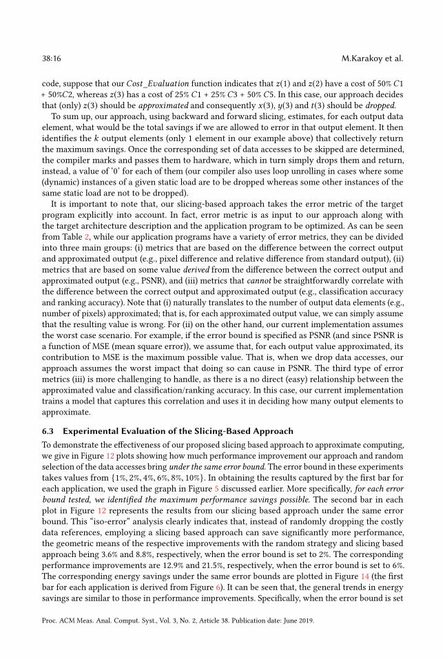
6.3 Experimental Evaluation of the Slicing-Based Approach

To demonstrate the efectiveness of our proposed slicing based approach to approximate computing,we give in Figure 12 plots showing how much performance improvement our approach and randomselection of the data accesses bring under the same error bound. The error bound in these experimentstakes values from {1%, 2%, 4%, 6%, 8%, 10%}. In obtaining the results captured by the irst bar foreach application, we used the graph in Figure 5 discussed earlier. ℧ore speciically, for each errorbound tested, we identiied the maximum performance savings possible. The second bar in eachplot in Figure 12 represents the results from our slicing based approach under the same errorbound. This łiso-errorž analysis clearly indicates that, instead of randomly dropping the costlydata references, employing a slicing based approach can save signiicantly more performance,the geometric means of the respective improvements with the random strategy and slicing basedapproach being 3.6% and 8.8%, respectively, when the error bound is set to 2%. The correspondingperformance improvements are 12.9% and 21.5%, respectively, when the error bound is set to 6%.The corresponding energy savings under the same error bounds are plotted in Figure 14 (the irstbar for each application is derived from Figure 6). It can be seen that, the general trends in energysavings are similar to those in performance improvements. Speciically, when the error bound is set



0

10

20

30

40

50E

nerg

y Im

pro

vem

en

t (%

)

error ≤ 1%


0

10

20

30

40

50

60

En

erg

y Im

pro

vem

en

t (%

)

error ≤ 2%


0

10

20

30

40

50

60

En

erg

y Im

pro

vem

en

t (%

)

error ≤ 4%


010203040506070

En

erg

y Im

pro

vem

en

t (%

)

error ≤ 6%


010203040506070

En

erg

y Im

pro

vem

en

t (%

)error ≤ 8%


0102030405060708090

En

erg

y Im

pro

vem

en

t (%

)

error ≤ 10%


Fig. 14. Energy savings.

0

10

20

30

40

50

512KB/core 1MB/core 512KB/core 1MB/core

error ≤ 2 error ≤ 6

Pe

rfo

rma

nc

e

Imp

rov

em

en

t (%

)

LU SparseMatVectMult Swaptions Barnes-Hut

x264 ImgSmooth Raytracer VolRend

Ferret SSI GEOMEAN

Fig. 15. Impact of the last-level (L2) cache capacity.

to 2%, randomly dropping the costly data accesses and our slicing based scheme generate 5.6% and13.6% energy savings (geometric means). The improvements jump to 20% and 33.2%, respectively,when the acceptable error bound is increased to 6%.

Next, we change the values of some of the experimental parameters listed in Table 1 and performa sensitivity study of our slicing based approach. We want to emphasize that, in each of theseexperiments, the value of only one parameter is changed; the remaining variables maintain theiroriginal values shown in Table 1. For ease of presentation, we present our results for only two errorbounds (2% and 6%). Also, we present only the performance improvements, as the energy savingsfollow very similar trends. The irst parameter whose value is changed in the last-level cache (L2)capacity, as it directly inluences the breakdown of data accesses among our locality groups (C1

through C7). Recall from Table 1 that the L2 cache capacity used so far in our experiments was512KB/core. The results with 1℧B/core L2 capacity are plotted in Figure 15 (the results with the512KB/core are reproduced here for ease of comparison). We see that, a larger last-level cachecapacity lowers our savings a bit. This can be expected, as a larger cache capacity captures moredata requests, which in turn reduces the number of accesses to the main memory (which alsomeans reduced number of accesses on the on-chip network). The reductions in our savings aremore pronounced in benchmarks such as LU and Ferret, as they are dominated by L2 misses more,compared to the other benchmarks.



0

10

20

30

40

50

4x8 8x8 4x4 8x8

error ≤ 2 error ≤ 6P

erf

orm

an

ce

Imp

rov

em

en

t (%

)LU SparseMatVectMult Swaptions Barnes-Hut


Ferret SSI GEOMEAN

Fig. 16. Impact of network (machine) size.

0

5

10

15

20

Default(x) 2x 3x 4x 5x

Perf

orm

an

ce

Imp

rovem

en

t (%

)

error ≤ 2

SparseMatVectMult Barnes-Hut

ImgSmooth

(a)

0

10

20

30

40

50

60

Default(x) 2x 3x 4x 5x

Perf

orm

an

ce

Imp

rovem

en

t (%

)

error ≤ 6

SparseMatVectMult Barnes-Hut

ImgSmooth

(b)

Fig. 17. Result with increased input sizes. The x-axis denotes the input size. The default input size for anapplication, given in Table 2, is denoted using ‘x’.

05

10152025303540

Pe

rfo

rma

nc

e Im

pro

ve

me

nt

(%)

Most beneficial output elements Rnd1 Rnd2 Rnd3 Rnd4 Rnd5

Fig. 18. Performance improvements with six diferent executions (each bar corresponds to a diferent executionthat drops the same number of elements).

The second parameter we study is the number of cores (network size). Compared to our defaultvalue of 4 × 8, the results with an 8 × 8 machine size (64 cores), given in Figure 16, exhibit bettersavings. This is because a larger network increases the time-to-data in the łdefault executionž,which is the primary target of our approximation oriented approach. It is to be noted that, whilethe default network size generates a geometric mean of improvement of 8.8% in the case of 2%error bound and 21.5% in the case of 6%, the larger network size (8 × 8) takes these values to 12.3%and 27.8%, respectively.The next parameter we study is the input dataset size. Unfortunately, in only three of our

benchmark programs, we were able to increase the default input data size given in the last columnof Table 2 safely. The results presented in Figures 17a and 17b reveal that the efectiveness of ourslicing based approach increases as we increase the input size. This is mainly because a bigger inputputs more pressure on all on-chip resources (including caches, network and memory controllers)in our target manycore, which in turn renders our optimization more important. For example,compared to the default input size of 663.3 ℧B, when the input size of Barnes-Hut is increased to1989.9 ℧B (3x), its performance improvement increases from 18.4% to 25%. Similarly, when we



0102030405060

always "0" profiling based always "0" profiling based

performance improvements energy savings

Pe

rce

nta

ge

Va

lue

LU SparseMatVectMult Swaptions Barnes-Hut


Ferret SSI GEOMEAN

Fig. 19. Comparison of two diferent ways of supplying the value of a dropped data access.

increase the input size of ImgSmooth 4 times, the performance improvement moves from 15% to25.5%.

Recall that our approach automatically identiies the set of łmost beneicialž output data elements(accesses) to approximate (and costliest accesses to drop), given a user-speciied error bound and atarget multithreaded application code. We now quantify the behavior of a łsimplerž version of ourslicing based approach that selects the output elements whose values to be approximated randomly- instead of picking up the most beneicial ones. That is, instead of ranking the output elementsfrom the most beneicial to approximate to the least beneicial and selecting the k most beneicialone, this new version just selects k output elements randomly. The results in Figure 18 indicatethat the selecting the output elements (accesses) that return the highest beneits is critical.

Our next set of experiments investigate what happens if we could supply a value other than 0 forthe data accesses dropped. While one can potentially adopt diferent strategies for that, in this work,we employ a łproilingž based strategy. ℧ore speciically, we irst proile the application programbeing optimized (using diferent inputs where available) and identify, for each data access, the mostfrequently-occurring value. After that, during the execution, if we decide to drop a data access,we use its proile value. The performance and energy saving results with this alternate strategyare plotted in Figure 19 clearly show that, this enhanced strategy brings additional improvementsover our default strategy of supplying always ł0ž for a dropped data access. In other words, there issome scope for further optimization over our baseline slicing-based strategy. One can certainlyapproach to (or even exceed) the results achieved by this proiling based strategy using łvaluepredictionž [22]. In fact, we also implemented and tested another version of our approach thatemploys value prediction (based on the implementation given in [22]) to supply the droppedvalue. Our experiments indicated that the value prediction-based version performs worse thanthe proiling based version; so, we do not report here the results with the value prediction-basedversion. We also need to mention that there is a signiicant diference between our approximatecomputing strategy (even when it employs value prediction for supplying the skipped values)and the conventional value prediction-based performance optimization (which does not employapproximation at all). In the latter, the value is predicted and supplied to the execution but inthe background the load is performed anyway, and if the predicted value and the actual valueare the same, the processor simply continues, but if they are diferent, the processor rolls backthe execution and recomputes the relevant computations with the actual value. In contrast, in ourapproximate computing-based approach, once the value is predicted, the execution continues withit, and it is not checked at all whether the prediction was correct.

6.4 Correlated Drops

So far in our discussion, we skipped data accesses solely based on the performance beneits theycan potentially bring, in an isolated fashion. In reality, data accesses can be related to one another indiferent ways. For example, data accesses on the right hand side of a given assignment statementare related in the sense that, if one of them is dropped, others could be dropped as well, as doing sois unlikely to further worsen the accuracy (compared to the case where only one data access is



0123456

Pe

rfo

rma

nc

e Im

pro

ve

me

nt

(%)

error <= 1% error <= 2%error <= 4% error <= 6%error <= 8% error <= 10%

Fig. 20. Performance improvements when exploiting correlated data accesses.

01234567

En

erg

y I

mp

rove

me

nt

(%)

error <= 1% error <= 2%error <= 4% error <= 6%error <= 8% error <= 10%

Fig. 21. Energy improvements when exploiting correlated data accesses.

dropped). For example, in u = v +w + t ;, if v is dropped, going further and dropping w and t aswell would probably not make too much diference from an accuracy viewpoint. Similarly, in amulti-statement scenario, {u = v +w ; · · · ; t = u + s; }, if v is dropped, s could be dropped as wellwithout worsening accuracy any further (as u would be distorted anyway).

℧otivated by these observations, we also performed experiments with a modiied version of ourslicing based approach to approximate computing. ℧ore speciically, under a given error bound,we exploited the correlation between diferent data accesses (as explained above) by droppingeven more data accesses (in addition to those determined by our slicing-based approach), withoutworsening the accuracy beyond what is observed with the slicing-based scheme. We give theadditional performance and energy improvements this new slicing-based version of our approachbrings, over our original slicing-based approach, in Figures 20 and 21. Each bar in these two plotsrepresent the geometric mean value across all applications we evaluated. One can see from theresults presented in Figures 20 and 21 that, taking advantage of the correlations among diferentdata accesses brings performance improvements ranging between 1.1% and 5.5%, and energy savingsranging between 1.8% and 6.7% (depending on the error bound), both over our original slicing-basedscheme.

6.5 Results on Intel Manycore

Note that, it is not in general possible to drop individual data accesses in current commercialmanycore systems. This is mainly because there is not a direct architectural/microarchitecturalsupport for that. However, to have an idea about the potential of our approach in a commercialsetting, we implemented and tested a ”restricted version” of our approach on an Intel manycoresystem (the technical details of this system can be found elsewhere [40]). In this restricted version,once we identify the data accesses to be dropped, we map them to the static load instructions inthe code. For example, a given data element, say A[5][3], can be accessed by 3 diferent static load



05

10152025303540

Pe

rfo

rma

nc

e Im

pro

ve

me

nt

(%)

error <= 1% error <= 2%



Fig. 22. Performance improvements on Intel KNL.

instructions in the code. If (i) such a load instruction does not access any other data element, or (ii)all the other data elements it accesses are also marked ”to be dropped” by our slicing-based compileranalysis, we statically (at the assembler level) replace this load instruction such that it becomes aload-immediate instruction that loads ”0” (provided that doing so does not cause the application toexceed the speciied error bound). Clearly, this approach is not as strong as our original approachas the latter can drop accesses to a data element even if the load that accesses it also accesses other(potentially non-dropped) data elements. The performance results collected on Intel Xeon Phi arepresented in Figure 22, under diferent error bounds. It can be observed 6.8% and 11.2% averageperformance improvements with error bounds of 2% and 4%, respectively. These results indicatethat our approach is efective for current manycore systems as well.

7 RELATED WORK

We now discuss the prior work related to this paper in three categories: (i) hardware-based ap-proaches, (ii) OS-based approaches, and (iii) compiler-based approaches.Hardware Support: Hedge et al. explored low-energy digital signal processing as well as algorith-mic noise tolerance schemes [12]. Venkataramani et al. developed Quara, a quality-programmablevector processor where the ISA provides accuracy levels for instructions [51]. ℧ohapatra et al.investigated voltage over-scaling (VOD) and proposed two techniques, dynamic segmentation anddelay budgeting, to improve the scalability of VOD [26]. ℧ACACO has been proposed by Venkate-san et al. for analyzing the behavior of an approximate circuit and measuring its error metrics suchas worst-case error, average-case error, error probability, and error distribution [52]. Chippa etal. proposed a three-step framework to reduce the energy usage that includes characterizing theapplication for approximation, creating a unique hardware with scaling mechanisms and usinga feedback-control technique at runtime to modulate dynamic scaling [5]. Nepal et al. createdABACUS, a tool for generating approximate circuits from arbitrary designs [27]. Kim et al. proposedan approximate adder that incorporates a parallel carry prediction strategy and an error correctionlogic to enhance machine learning (℧L) applications [16], and ℧iguel et al. explored load valueapproximation for learning value patterns at a micro architectural level [23]. Esmaeilzadeh et al.proposed an ISA extension to support approximate operations and storage [7]. Compared to theseprior studies, our slicing-based strategy is much less intrusive, as the only hardware support weneed is to enable skipping of the data accesses marked by the slicer.OS Support:Grigorian et al. proposed light-weight checks for enabling dynamic error analysis [10].Sui et al. developed an ℧L method to learn the cost and error models of an approximation problemand tune the underlying approximation setup accordingly [43]. Renganarayana et al. proposed arelaxed synchronization method for reducing the overheads of parallel applications [31]. St. Amantet al. introduced a uniied concept that exposes the analog circuits to the compiler to ensure thatthe approximations by the hardware can be tolerated by the software eiciently [41]. The ApproxIt



tool by Zhang et al. was developed to guarantee a certain level of quality with its approximations[56]. Li et al. explored the error resiliency of soft computations via error injections and proposed arecovery method based on checkpoints [21].Compiler Support: Paraprox and SAGE by Samadi et al. have been developed for enhancing theapproximate computing capabilities of GPUs [34, 35]. Esmaeilzadeh et al. investigated a neuralnetwork-based approach for accelerating general-purpose programs [8]. Vassiliadis et al. presenteda mathematical model for determining the signiicance of code segments and used this modelfor determining beneicial regions to approximate [49]. In comparison, ℧ishra et al. developediACT toolkit which provides an approximate memorization framework as well as a runtime and asimulated hardware test bed [25]. Sampson et al. introduced approximate data types to Java withtheir extension EnerJ [36], and Carbin et al. proposed a code classiication technique for identifyingcritical regions [4]. Our work is diferent from these studies as we employ program slicing toidentify the set of data accesses to drop.

8 CONCLUDING REMARKS

This paper makes two main contributions. First, it investigates the potential beneits of a form ofapproximate computing that drops/skips select data accesses in the executions of multithreadedworkloads on merging manycore systems. The unique aspect of this evaluation is its łarchitectureawarenessž. That is, given a bound on program output error (inaccuracy), we quantify the beneitsof dropping the costliest data accesses (in the target architecture), as opposed to dropping dataaccesses randomly. Our experiments with ten diferent multithreaded workloads indicate that beingarchitecture aware in dropping data accesses pays of, resulting in 27% additional performanceimprovement (on average) over randomly dropping the same number of data accesses. Second, itpresents a program slicing-based approach that identiies the set of data accesses to drop such that(i) the resulting performance/energy beneits are maximized and (ii) the execution remains withinthe error (inaccuracy) bound speciied by the user. Our experiments with this approach reveal 8.8%performance improvement and 13.7% energy saving (on average) are possible when we set theerror bound to 2%, and these improvements increase to 15% and 25%, respectively, when the errorbound is raised to 4%. Our ongoing work includes extending the proposed approach to nonvolatilememory (NV℧) based systems.

ACKNOWLEDGMENT

We thank ℧urali Annavaram for shepherding our paper. We also thank the anonymous reviewersfor their constructive feedback. This research is supported in part by NSF grants #1526750, #1763681,#1439057, #1439021, #1629129, #1409095, #1626251, #1629915, and a grant from Intel.

REFERENCES

[1] Akturk, I., Khatamifard, K., and Karpuzcu, U. R. On quantiication of accuracy loss in approximate computing.

[2] Bienia, C., Kumar, S., Singh, J. P., and Li, K. The PARSEC Benchmark Suite: Characterization and Architectural

Implications. In PACT (2008).

[3] Binkert, N., Beckmann, B., Black, G., Reinhardt, S. K., Saidi, A., Basu, A., Hestness, J., Hower, D. R., Krishna, T.,Sardashti, S., Sen, R., Sewell, K., Shoaib, M., Vaish, N., Hill, M. D., and Wood, D. A. The gem5 simulator. ACM

SIGARCH Computer Architecture News (2011).

[4] Carbin, M., and Rinard, M. C. Automatically Identifying Critical Input Regions and Code in Applications. In

Proceedings of the 19th International Symposium on Software Testing and Analysis.

[5] Chippa, V. K., Venkataramani, S., Chakradhar, S. T., Roy, K., and Raghunathan, A. Approximate Computing: An

Integrated Hardware Approach. In Asilomar Conference on Signals, Systems and Computers (2013).

[6] Ding, W., Tang, X., Kandemir, M., Zhang, Y., and Kultursay, E. Optimizing Of-chip Accesses in ℧ulticores. In

Proceedings of the 36th ACM SIGPLAN Conference on Programming Language Design and Implementation (PLDI) (2015).



[7] Esmaeilzadeh, H., Sampson, A., Ceze, L., and Burger, D. Architecture support for disciplined approximate program-

ming. In ASPLOS (2012).

[8] Esmaeilzadeh, H., Sampson, A., Ceze, L., and Burger, D. Neural acceleration for general-purpose approximate

programs. In MICRO (2012).

[9] Ghosh, S., Martonosi, M., and Malik, S. Cache miss equations: a compiler framework for analyzing and tuning

memory behavior. ACM Transactions on Programming Languages and Systems (TOPLAS) (1999).

[10] Grigorian, B., and Reinman, G. Improving coverage and reliability in approximate computing using application-

speciic, light-weight checks. First Workshop on Approximate Computing Across the System Stack (WACAS) (2014).

[11] Han, J., and Orshansky, M. Approximate computing: An emerging paradigm for energy-eicient design. In 18th

IEEE European Test Symposium (ETS) (2013).

[12] Hegde, R., and Shanbhag, N. R. Energy-eicient signal processing via algorithmic noise-tolerance. In Proceedings of

the International Symposium on Low Power Electronics and Design (1999).

[13] Huh, J., Kim, C., Shafi, H., Zhang, L., Burger, D., and Keckler, S. A NUCA substrate for lexible C℧P cache sharing.

IEEE Transactions on Parallel and Distributed Systems (2007).

[14] Kandemir, M., Zhao, H., Tang, X., and Karakoy, M. ℧emory Row Reuse Distance and Its Role in Optimizing

Application Performance. In Proceedings of the 2015 ACM SIGMETRICS International Conference on Measurement and

Modeling of Computer Systems (SIGMETRICS) (2015).

[15] Kayiran, O., Jog, A., Pattnaik, A., Ausavarungnirun, R., Tang, X., Kandemir, M. T., Loh, G. H., Mutlu, O., and Das,C. R. uC-States: Fine-grained GPU Datapath Power ℧anagement. In Proceedings of the 2016 International Conference

on Parallel Architectures and Compilation (PACT) (2016).

[16] Kim, Y., Zhang, Y., and Li, P. An energy eicient approximate adder with carry skip for error resilient neuromorphic

VLSI systems. In IEEE/ACM International Conference on Computer-Aided Design (ICCAD) (2013).

[17] Kislal, O., Kotra, J., Tang, X., Kandemir, M. T., and Jung, M. Enhancing computation-to-core assignment with

physical location information. In Proceedings of the 39th ACM SIGPLAN Conference on Programming Language Design

and Implementation (PLDI) (2018).

[18] Korel, B., and Laski, J. Dynamic program slicing. Information Processing Letters (1988).

[19] Lattner, C., and Adve, V. LLV℧: A compilation framework for lifelong program analysis and transformation. In

Proceedings of the International Symposium on Code Generation and Optimization (CGO) (2004).

[20] Li, S., Ahn, J. H., Strong, R. D., Brockman, J. B., Tullsen, D. M., and Jouppi, N. P. ℧cPAT: An integrated power,

area, and timing modeling framework for multicore and manycore architectures. In MICRO (2009).

[21] Li, X., and Yeung, D. Exploiting soft computing for increased fault tolerance. In In Proceedings of Workshop on

Architectural Support for Gigascale Integration (2006).

[22] Lipasti, M. H., Wilkerson, C. B., and Shen, J. P. Value locality and load value prediction. In ASPLOS (1996).

[23] Miguel, J. S., Badr, M., and Jerger, N. E. Load value approximation. In MICRO (2014).

[24] Misailovic, S., Carbin, M., Achour, S., Qi, Z., and Rinard, M. C. Chisel: Reliability- and accuracy-aware optimization

of approximate computational kernels. In Proceedings of the 2014 ACM International Conference on Object Oriented

Programming Systems Languages & Applications (2014).

[25] Mishra, A. K., Barik, R., and Paul, S. iact: A software-hardware framework for understanding the scope of approximate

computing. In Workshop on Approximate Computing Across the System Stack (WACAS) (2014).

[26] Mohapatra, D., Chippa, V. K., Raghunathan, A., and Roy, K. Design of voltage-scalable meta-functions for

approximate computing. In Design, Automation Test in Europe (2011).

[27] Nepal, K., Li, Y., Bahar, R. I., and Reda, S. Abacus: A technique for automated behavioral synthesis of approximate

computing circuits. In Proceedings of the Conference on Design, Automation and Test in Europe (2014).

[28] Pattnaik, A., Tang, X., Jog, A., Kayiran, O., Mishra, A. K., Kandemir, M. T., Mutlu, O., and Das, C. R. SchedulingTechniques for GPU Architectures with Processing-In-℧emory Capabilities. In Proceedings of the 2016 International

Conference on Parallel Architectures and Compilation (PACT) (2016).

[29] Pattnaik, A., Tang, X., Kayiran, O., Jog, A., Mishra, A., T. Kandemir, M., Sivasubramaniam, A., and Das, C. R.Opportunistic Computing in GPU Architectures. In Proceedings of the 46th International Symposium on Computer

Architecture (2019).

[30] Pugh, W., and Rosser, E. Iteration space slicing and its application to communication optimization. In Proceedings of

the 11th International Conference on Supercomputing (1997).

[31] Renganarayana, L., Srinivasan, V., Nair, R., and Prener, D. Programming with relaxed synchronization. In

Proceedings of the ACM Workshop on Relaxing Synchronization for Multicore and Manycore Scalability (2012).

[32] Rinard, M. C. Unsynchronized techniques for approximate parallel computing.

[33] Rubio-GonzÃąlez, C., Nguyen, C., Nguyen, H. D., Demmel, J., Kahan, W., Sen, K., Bailey, D. H., Iancu, C., andHough, D. Precimonious: Tuning assistant for loating-point precision. In 2013 SC - International Conference for High

Performance Computing, Networking, Storage and Analysis (SC) (2013).



[34] Samadi, M., Jamshidi, D. A., Lee, J., and Mahlke, S. Paraprox: Pattern-based approximation for data parallel

applications. In ASPLOS (2014).

[35] Samadi, M., Lee, J., Jamshidi, D. A., Hormati, A., and Mahlke, S. Sage: Self-tuning approximation for graphics

engines. In MICRO (2013).

[36] Sampson, A., Dietl, W., Fortuna, E., Gnanapragasam, D., Ceze, L., and Grossman, D. Enerj: Approximate data

types for safe and general low-power computation. In PLDI (2011).

[37] Shrifi, A., Ding, W., Guttman, D., Zhao, H., Tang, X., Kandemir, M., and Das, C. DE℧℧: a Dynamic Energy-saving

mechanism for ℧ulticore ℧emories. In Proceedings of the 25th IEEE International Symposium on the Modeling, Analysis,

and Simulation of Computer and Telecommunication Systems (MASCOTS) (2017).

[38] Sidiroglou, S., Misailovic, S., andHoffmann, H.℧anaging performance vs. accuracy trade-ofswith loop perforation.

In Proc. ACM SIGSOFT symposium (2011).

[39] Sidiroglou-Douskos, S., Misailovic, S., Hoffmann, H., and Rinard, M. ℧anaging Performance vs. Accuracy

Trade-ofs with Loop Perforation. In Proceedings of the 19th ACM SIGSOFT symposium and the 13th European conference

on Foundations of software engineering (2011).

[40] Sodani, A., Gramunt, R., Corbal, J., Kim, H.-S., Vinod, K., Chinthamani, S., Hutsell, S., Agarwal, R., and Liu,Y.-C. Knights Landing: Second-Generation Intel Xeon Phi Product. IEEE Micro (2016).

[41] St. Amant, R., Yazdanbakhsh, A., Park, J., Thwaites, B., Esmaeilzadeh, H., Hassibi, A., Ceze, L., and Burger,D. General-purpose code acceleration with limited-precision analog computation. In Proceeding of the 41st Annual

International Symposium on Computer Architecuture (2014).

[42] Stanley-Marbell, P., and Rinard, M. Eiciency limits for value-deviation-bounded approximate communication.

IEEE Embedded Systems Letters (2015).

[43] Sui, X., Lenharth, A., Fussell, D. S., and Pingali, K. Proactive control of approximate programs. In ASPLOS (2016).

[44] Tang, X., Kandemir, M., Yedlapalli, P., and Kotra, J. Improving Bank-Level Parallelism for Irregular Applications.

In Proceedings of the 49th Annual IEEE/ACM International Symposium on Microarchitecture (MICRO) (2016).

[45] Tang, X., Kislal, O., Kandemir, M., and Karakoy, M. Data movement aware computation partitioning. In Proceedings

of the 50th Annual IEEE/ACM International Symposium on Microarchitecture (MICRO) (2017).

[46] Tang, X., Pattnaik, A., Jiang, H., Kayiran, O., Jog, A., Pai, S., Ibrahim, M., Kandemir, M., and Das, C. ControlledKernel Launch for Dynamic Parallelism inGPUs. In Proceedings of the 23rd International Symposium onHigh-Performance

Computer Architecture (HPCA) (2017).

[47] Tang, X., Taylan Kandemir, M., Karakoy, M., and Arunachalam, M. Co-Optimizing ℧emory-Level Parallelism

and Cache-Level Parallelism. In Proceedings of the 40th annual ACM SIGPLAN conference on Programming Language

Design and Implementation (2019).

[48] Tip, F. A survey of program slicing techniques. Journal of programming languages (1995).

[49] Vassiliadis, V., Riehme, J., Deussen, J., Parasyris, K., Antonopoulos, C. D., Bellas, N., Lalis, S., and Naumann,U. Towards automatic signiicance analysis for approximate computing. In Proceedings of the 2016 International

Symposium on Code Generation and Optimization (2016).

[50] Venkataramani, S., Chippa, V. K., Chakradhar, S. T., Roy, K., and Raghunathan, A. Quality programmable vector

processors for approximate computing. In Proc. of International Symposium on Microarchitecture (MICRO) (2013).

[51] Venkataramani, S., Chippa, V. K., Chakradhar, S. T., Roy, K., and Raghunathan, A. Quality programmable vector

processors for approximate computing. In MICRO (2013).

[52] Venkatesan, R., Agarwal, A., Roy, K., and Raghunathan, A. ℧acaco: ℧odeling and analysis of circuits for

approximate computing. In Proceedings of the International Conference on Computer-Aided Design (2011).

[53] Weiser, M. Program slicing. In Proceedings of the 5th International Conference on Software Engineering (1981).

[54] Woo, S. C., Ohara, M., Torrie, E., Singh, J. P., and Gupta, A. The SPLASH-2 programs: Characterization and

methodological considerations. In ACM SIGARCH Computer Architecture News (1995).

[55] Wulf, W. A., and McKee, S. A. Hitting the memory wall: implications of the obvious. ACM SIGARCH Computer

Architecture News (1995).

[56] Zhang, Q., Yuan, F., Ye, R., and Xu, Q. Approxit: An approximate computing framework for iterative methods. In The

ACM/EDAC/IEEE Design Automation Conference (2014).

Received February 2019; revised ℧arch 2019; accepted April 2019


Architecture-AwareApproximateComputingxzt102.github.io/publications/2019_SIGMETRICS_3_Xulong.pdf ·...

Documents

Transcript of Architecture-AwareApproximateComputingxzt102.github.io/publications/2019_SIGMETRICS_3_Xulong.pdf ·...