Journal of lntrrnationaf ,Cloney and Finance (1988). 7, J29--1Jj

Arbitrage Boundaries, Treasury Bills, and Covered Interest Parity

GEOFFREY POITR.S*

Bank of Canada, Ottawa, Ontario, Canada K IA OG9

This paper uses the covered interest parity relationship to define upper and lower arbitrage boundaries on domestic Treasury bill (r-bill) rates. Adapting the methodology for estimating frontier functions, empirical tests are specified to determine whether the arbitrage boundaries provide a binding constraint on the behavior of the domestic t-bill rate. Empirical evidence is presented for the covered Canadian t-bill rate which indicates that at various times the US t-bill rate has been a binding lower boundary and the Euro-US dollar deposit rate has provided a binding upper boundary.

For non-Euromarket instruments, various studies have identified significant deviations of forward rates from their covered interest parity (CIP) levels (e.g., Frenkel and Levich, 1975,1977,1981; Otani and Tiwari, 1981; Bahmani-Oskooee and Das, 1985; Sharpe, 1985; Overturf, 1986). Past studies have attempted to explain these deviations in various ways: transactions costs, imperfect substitutability, announcement effects, political risk and so on. Most of these

studies have, implicitly or explicitly, been based on the assumption that the CIP arbitrage relationship holds as an equality. However, in the case of the Treasury bill (t-bill) market, covered interest arbitrage provides inequality restrictions because arbitrageurs are unable to borrow at the t-bill rate. If binding, these inequality restrictions can be used for various purposes such as formulating speculative trading strategies or as a guide for policymakers to setting a level for domestic interest rates compatible with external equilibrium.1

In the following, Section I provides an explanation of two covered interest arbitrage trades which affect the t-bill market. It is demonstrated that covered interest arbitrage can be used to provide both lower and upper arbitrage boundaries on domestic t-bill rates. Section II discusses the estimation procedures for equations subject to a one-sided boundary. Adapting the methodology for estimating frontier functions, it is demonstrated that if the arbitrage boundary is binding then the CIP regression residuals will exhibit non-normal skewness.

* The arbitrage discussed in this paper was first brought to the author’s attention by an anonymous

money market trader. Helpful comments were received by Robert LaFrance, Bob Hannah, F.

Caramazza, John AMurray, and the referees. Scott Colbourne provided able research assistance. The

views presented in this paper are solely the author’s and are not intended to represent the position of the Bank of Canada.

0261-5606!88/04/0429-17SO3.00 C 1988 Butterworth & Co (Publishers) Ltd

430 .Irbitragr Boundaries, Trrasur_v Bills, and Coverrd lntmst Parig

Section III provides regression evidence on the validit): of the boundary behavior hypothesis for the Canadian t-bill market. X number ot different specifications for the CIP deviations are examined together with a variety of distributional tests. Section IV provides a summary of the relevant results contained in the paper.

I. The Arbitrage Relationships

In markets where arbitrage is active and unrestricted, the net return offered on a hedged basis by an instrument denominated in foreign currency should approximately equal the rate offered by a similar instrument denominated in domestic currency. This is the basis of CIP. For arbitrage involving securities

identical in all respects except currency denomination, the simplified CIP

relationship is often stated in one of two equivalent annualized forms:

(1) F 1 +i -=- S 1 +i*’

OK

(2) F-S i-i*

S 1 +i*’

where F = the 1 -year forward exchange rate in domestic direct terms,* S = the spot exchange rate in domestic direct terms, i=the domestic interest rate (on a 365-day basis), i* =the foreign interest rate (on a 365-day basis).

Even though for institutional reasons (1) and (2) may not be exact, these formulations are conventional in academic studies of CIP.3 Further, it is usually assumed that iand i* refer to the same type ofasset. However, when these assets are t-bills issued by different sovereign entities, the two securities involved will not typically have the same risk characteristics.

For the t-bill market, many of the earlier studies of CIP (e.g., Grubel, 1966; Bransonl969; Prachowny, 1970; Frenkel and Levich, 1975,1977) assumed that the equality in (1) and (2) arises from a combination of investor (i.e., asset holder)

determination of CIP and perfect substitutability of foreign and domestic t-bills (e.g., Frenkel and Levich, 1977, p. 1211, n. 2). If there is perfect substitutability then deviations from CIP will lead to investors selling the lower yielding t-bill and purchasing the higher yielding t-bill, fully covering any currency exposure. Unfortunately, this explanation makes the unsupportable assumption of perfect substitutability between foreign and domestic t-bills. In the US-Canadian case, for example, US t-bills are perceived differently by the market than Canadian t-bills due to taxation, liquidity and other risk factors. 4 Hence, substitution between US and Canadian t-bills by asset holders would be based on covered parity plus an adjustment for the differential characteristics of the two instruments.

In addition to differential characteristics driving deviations from the covered parity equality, the reliance on asset holder substitutability to maintain covered arbi- trage ignores the important role that the ability to borrow plays in certain types of covered interest arbitrage trades. More recent treatments of CIP have recognized the key role of arbitrageurs in maintaining CIP (e.g., Deardorff, 1979; Kreicher,

1982; Clinton, 1988). In this case, for the equality in (1) and (2) to hold covered interest arbitrageurs must have the ability, excluding transactions costs, to lend and

GEOFFREY POrTRAs 431

borrow at both i and i*. However, in the r-bill market arbitrageurs can lend, but not borrow, at the t-bill rate. Hence, where either ior i* is a t-bill rate, it is difficult to support the assumption of equality in (1) or (2) on arbitrage gr0unds.s When

both i and i* are t-bill rates, ability to borrow cannot play a key role and covered parity relations are determined both directly by asset holder substitution and indirectly through activity in other money market instruments. For present purposes, a covered parity relationship not directly affected by the borrowing activities of arbitrageurs will be referred to as a ‘risk arbitrage’.

In practice, a ‘pure’ covered interest arbitrage trade involves borrowing in one market and simultaneously investing on a fully covered basis in another market. The bulk of participants engaged in this covered interest arbitrage activity are the large

international commercial and investment banks. These banks have ready access to borrowed funds through the inter-bank Euro-currency deposit market. As a result of the relative ease with which covered interest arbitrage trades can be done in the Euro-currency deposit market, Euro-deposit rates for currencies other than the US dollar are closely tied to Euro-US rates through CIP (e.g., Marston, 1976; Husted and Kitchen, 1985).6 Hence, a key borrowing rate available for arbitrageurs doing covered interest arbitrage trades is the Euro-US rate. This ready availability of arbitrage funds at the Euro-US rate defines an arbitrage relationship between Euro-US rate and other non-Euro-currency assets. i For example, in the case oft- bills, whenever the covered domestic t-bill rate rises above the Euro-US rate arbitrageurs will borrow funds at the Euro-US rate, convert the funds into domestic dollars and purchase domestic t-bills. At the same time, the amount of funds to be received upon maturity of the t-bill will be covered forward. If the maturity of the t-bill and the Euro-deposit are the same, i.e., the arbitrageur does not try to ‘ride the yield curve’ to pick up additional basis points, the trade will generate a relatively riskless profit. This arbitrage establishes an upper bound on the domestic t-bill rate-the covered Euro-US deposit rate.

For equality to hold in (1)and (2) h t e arbitrage must be ‘two-sided’. Khile the arbitrage trade when the domestic t-bill rate exceeds the Euro-US rate is apparent,

the arbitrage trade for the Euro-US rate esceeding the domestic t-bill rate is not so clear. In this case, when the t-bill rate falls below the covered Euro-US rate, the implied covered interest arbitrage trade would involve borrowing at the domestic t-bill rate, converting to US dollars and buying Euro-currency deposits- simultaneously covering forward the funds to be received at the maturity of the Euro-US deposit. This trade cannot be executed because only the domestic government has the ability to issue liabilities in the domestic t-bill market. Hence, covered interest arbitrage only provides an upper boundary on t-bill rates. Based

on this analysis, it follows that for the t-bill market (2) must be restated as:

(3) F-S > i-i* -,- S 1 +i*’

where, for present purposes, i is the domestic t-bill rate and i* is the Euro-US dollar rate. Manipulation gives the following expression in terms of domestic t-bill rates:

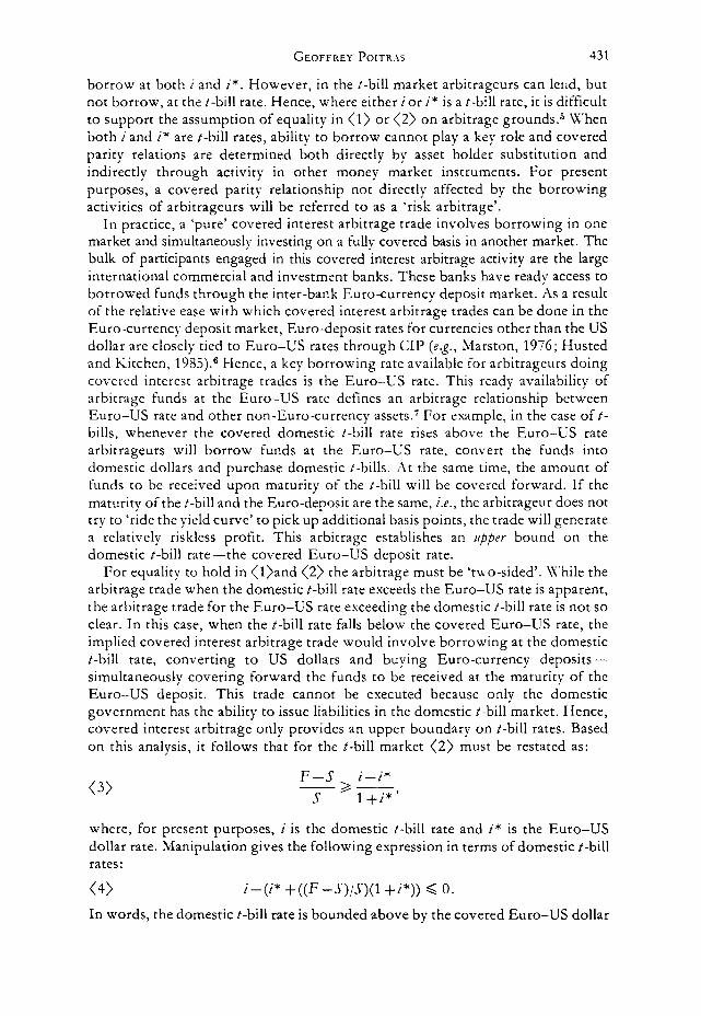
(4) i-(i* +((F-S)/S)(l +i*)) < 0.

In words, the domestic t-bill rate is bounded above by the covered Euro-US dollar

332

0.2

%

0.0

-0.2

-0.4

-0.6 I

-Arbitrage Boundaries, Treasury Bib, and Cocrrrd Intrrrst Parig

I J~II~~~~LL_ddII~II IIIIIIII~II ll~fl~ll~ll II~II~II~II II~II~II~II Il~lI~II~l 1980 1981 1982 1983 1984 1985 1986

L.

0.2

0.0

-0.2

-0.1

-0.6

CIPEUPO: I-(I.+((f-Q/S) ((+I-))

FIGURE 1.

rate. There is not strict equality because arbitrageurs are unable to borrow at the domestic t-bill rate. Figure 1 provides a plot of the deviations of the Canadian t-bill rate from the covered Euro rate for the 90-day maturity over the full sample examined in Section III.

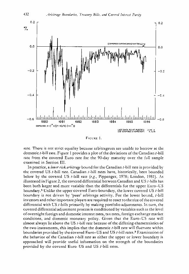
In practice, a lower risk arbitrage bound for the Canadian t-bill rate is provided by the covered US t-bill rate. Canadian t-bill rates have, historically, been bounded below by the covered US t-bill rate (e.g., Pippenger, 1978; London, 1981). As illustrated in Figure 2, the covered differential between Canadian and US t-bills has been both larger and more variable than the differentials for the upper Euro-US boundary.* Unlike the upper covered Euro-boundary, the lower covered US t-bill boundary is not driven by ‘pure’ arbitrage activity. For the lower bound, t-bill investors and other important players are required to react to the size of the covered differential with US t-bills primarily by making portfolio adjustments. In turn, the covered differential adjustment process is conditioned by variables such as the level of overnight foreign and domestic interest rates, tax rates, foreign exchange market conditions, and domestic monetary policy. Given that the Euro-US rate will almost always lie above the US t-bill rate because of the differing characteristics of the two instruments, this implies that the domestic t-bill rate will fluctuate within boundaries provided by the covered Euro-US and US t-bill rates.g Examination of the behavior of the Canadian t-bill rate as either the upper or lower boundary is approached will provide useful information on the strength of the boundaries provided by the covered Euro-US and US t-bill rates.

GEOFFREY Porr~.~s 433

1.0

70

0.8

0.6

0.4

0.2

0.0 LL ,,, r _

1980 1981 1982 1983 1984 1985 1986

1.0

0.8

0.6

CIPTB90: I-(l*+((F-S)/S)(l+l-))

II. Estimation Procedures

From an estimation standpoint, if a boundary is binding, then the CIP relationship is a special case of a ‘frontier’ function (Aigner et al., 1977; Forsund et al., 1980). Frontier function estimation occurs in a number of contexts in econometrics such as profit functions, production functions, and cost functions. In general, estimation of a frontier function is problematic because the functional relationship is bounded in one direction .l” As typically sp ecified, this results in equation residuals that are skewed (not symmetric) -violating conventional assumptions made for either ordinary least squares or Gaussian maximum likelihood estimation.

More formally, as in Olson et al. (1980) and others, the frontier estimation

problem starts with the general linear model specification:

(5) 4’ = Xb+e

where_y and e are T x 1 vectors of the endogenous variable and the residual, X is a T xk matrix of exogenous variables and b is the k x 1 parameter vector. Conventional OLS restrictions are imposed on X. Assuming the frontier restriction places an +per bound on (5), the residual in (5) is typically modelled as:

(6) e=v-_lt/j

where Y is i.i.d. N(0, c,‘) and tl is i.i.d. N(0, g), i.e., IHI is half-normal i.i.d. N(0, cri).

434 .-lrbitrage Bouudarits, Trrastlrr Biih. ami Cowrrd ln:<r<st Parit)

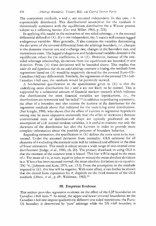
The component residuals, u and u, are assumed independent. In this case, e is exponentially distributed. This distributional assumption for the residuals is theoretically consistent with the equilibrium distribution for a Wiener process subject to a reflecting barrier (Cos and hliller, 1965, p. 225).

In applying this model to the estimation of one-sided arbitragey is the covered differential defined in (4). Ify is not independent, the Smatris will contain lagged

endogenous variables. hIore generally, X also contains the variables determining the deviation of the covered differential from the arbitrage boundary, i.e., changes

in the domestic interest rate and exchange rate, changes in the boundary rate, and transactions costs. The lagged endogenous and fundamental variables determine the equilibrium values for the coefficients, 6, in (5). However, because of the one- sided arbitrage relationship, deviations from the equilibrium are bounded in one direction. From (4) these deviations will be bounded above. This implies that nuder the null bypothens that the one-&led arbitrage constraint is bituhg, the residuals from regressions based on (4) would be negatively skewed for the covered Euro-US- Canadian t-bill rate differentials. Similarly, for regressions of the covered US t-bill- Canadian t-bill case, the residuals would be positively skewed.

A fundamental qualification to the specitication given in (6) is that the

underlying error distributions for v and tl are not likely to be normal. This is supported by a substantial amount of financial markets research which indicates that distributions for most financial variables are leptokurtotic, i.e., the distributions are symmetric and ‘fat-tailed’.” In addition to producing asymmetry, the effect of a boundary may also increase the kurtosis of the distribution for the regression residuals above that indicated for the underlying error distributions.

(See Knight, 1986, who shows that the effect of kurtosis in regression hypothesis

testing may be more important statistically than the effect of skewness.) Because

conventional tests of distributional shape are typically predicated on the assumption of i.i.d. normal random variables, it is useful to examine not only the

skewness of the distribution but also the kurtosis in order to provide more complete information about the possible presence of boundary behavior.

Regarding estimation, the specification in (6) defines the error term to be non- normal. Under the assumed deviation from normality, OLS estimates for all elements of b excluding the constant term will be unbiased and efficient in the class of linear estimators. This result is robust across a wide range of non-normal error distributions (Judge, et a/., 1985, ch. 20). The primary drawback to using OLS is that the estimate of the constant term is biased. This bias will be equal to the mean of e. The mean of e is, in turn, equal to (plus or minus) the mean absolute deviation in CI. When IA has been assumed normal, the mean absolute deviation in CI is equal to:

(27~)’ ‘G, (Johnson and Katz, 1970, sec. 13.3). From the assumption on the residuals imposed in (6), this bias will be negative. With some effort, it can further be shown that the closed form espression for G, depends on the third moment of the OLS residuals (Olsen, et al., p. 69; Waldman, 1982).”

III. Empirical Evidence

This section provides regression evidence on the effect of the CIP boundaries on Canadian t-bill rates.r3 As noted, the upper and lower covered boundaries on the Canadian t-bill rate impose qualitatively different one-sided restrictions: the Euro- US boundary is determined by ‘pure’ arbitrage while the US t-bill boundary is

GEOFFREY PorrR.~j 435

determined by risk arbitrage. In order to identify possible maturity effects, weekly data for 30- and 90-day maturities are examined over the 1980-86 period. All rates are adjusted to reflect actual returns over the holding period. Based on examination of Figures 1 and 2, the sample can be divided into three distinct parts: the 1980-82 period of high and volatile US and Canadian interest rates, the 1983-84 period of stable rates and the 1985-86 period of stable to declining interest rates. In the earlier subsample, volatility in the covered differential was two to three times larger than in the later subsamples. For the Euro-US case, covered differentials during this period varied between +8 to -54 basis points. 1-L Covered differentials during the

latter two periods varied between 0 and -22 basis points. To get a rough idea of the distributional properties of the covered differentials,

distributional statistics for both the Canadian t-bill-covered Euro (CDE) and the Canadian t-bill-covered US t-bill (CDT) cases were examined. For both the CDE and CDT cases, skewness was highly significant and of the expected sign for the full sample (as was kurtosis). More precisely, it was not possible to accept the null hypothesis of symmetric (or normally distributed) residuals for the full samples. Compared to the CDT case, the mean values for CDE were about one-half the value of CDT and of opposite sign. Regarding the subsample results, when both maturities for the 1985-86 subsample were excluded, non-normal skewness was observed for the CDT case. (For all cases, kurtosis was non-normal.) For CDE, with the exception of the 90-day maturity for the 1980-82 sample, the null hypothesis of symmetry and normality was rejected. Unfortunately, these theoretically favorable distributional results must be qualified due to presence of persistence in the residuals. Significant estimates for first- and higher-order autocorrelation coefficients were observed with the AR(l) coefficients varying between 0.5 and 0.8.

The presence of residual autocorrelation poses a number of estimation problems. Khile there is little theoretical or empirical work directly on the subject of testing distributional properties for dependent random variables, the distributional tests reported here will, theoretically, be biased against the null hypothesis of normally distributed residuals when the residuals are serially correlated.‘j This follows because the formulae for the standardized sample moments are based on the assumption of independence and are biased estimates when the random variables are dependent. For example, it is well known that the conventional estimate of the second moment of the OLS residuals is biased when the residuals are serially correlated. (Hence, the studentized range is biased.) Because the second moment is used in calculating the standardized sample moments, unless the bias in the numerator and the denominator cancels out the distributional tests reported here will be biased.

In order to correct for the residual persistence, it is useful to identify its source(s). Evidence that the time series process for the residuals is of higher (i.e., greater than 2) order indicates that a primary source of the persistence is due to the use of ‘overlapping’ data (e.g., Hansen and Hodrick, 1980; Stockman, 1978). In other words, the weekly sampling frequency is shorter than the length of the contracts (30 and 90 days) used to calculate the covered differentials. In this case, the implied error structure is a moving average process with order dependent on the extent of the overlap. This insight allows the problem of dependency in the covered differentials to be addresed in an OLS framework by fitting an AR model for the covered differentials.16 The resulting OLS residuals are then used in the

436 .-lrbitragr Boundaries, Treasury Bills, and Cowred Intrrrrt Parity

TABLE 1. CDE, = .-1(L)CDE,_,.

%? SR

Order of the

;\R model

Sample SO W2SS6W-73

30-day go-day

Sample 80 W-3%-82 WY2

30-day go-day

SampLe 53 W 1-H WY2

30-day go-day

Sample 8iWl-86W2J

30-day go-day

-0.47839' -0.3933*

-0.18852 - 0.04595

-0.59114* - 0.5534*

-0.48298* - 1.03*

2.7390* 1.95*

0.71408* 0.07612

2.80* 0.7283*

0.73245* 1.31’

107.68* 56.7*

3.5049 5.8932* 0.076552 5.8898*

40.03* 7.61*

4.5311* 18.25*

7.8262+ 7.988+

7.25* 5.57

5.6704* 5.41

2 2

2 2

2 2

2 2

iVote: An asterisk indicates significance at the 10 per cent level. b2 =0 under the null hypothesis.

distributional tests. Because these OLS residuals will be serially uncorrelated by construction, both the third and fourth standardized sample moments and the estimate of the residual variance will be unbiased.

The AR model to be estimated is defined to be:*’

(7) CD, = A(L)CD,_, +e,,

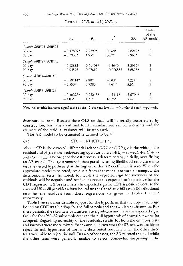
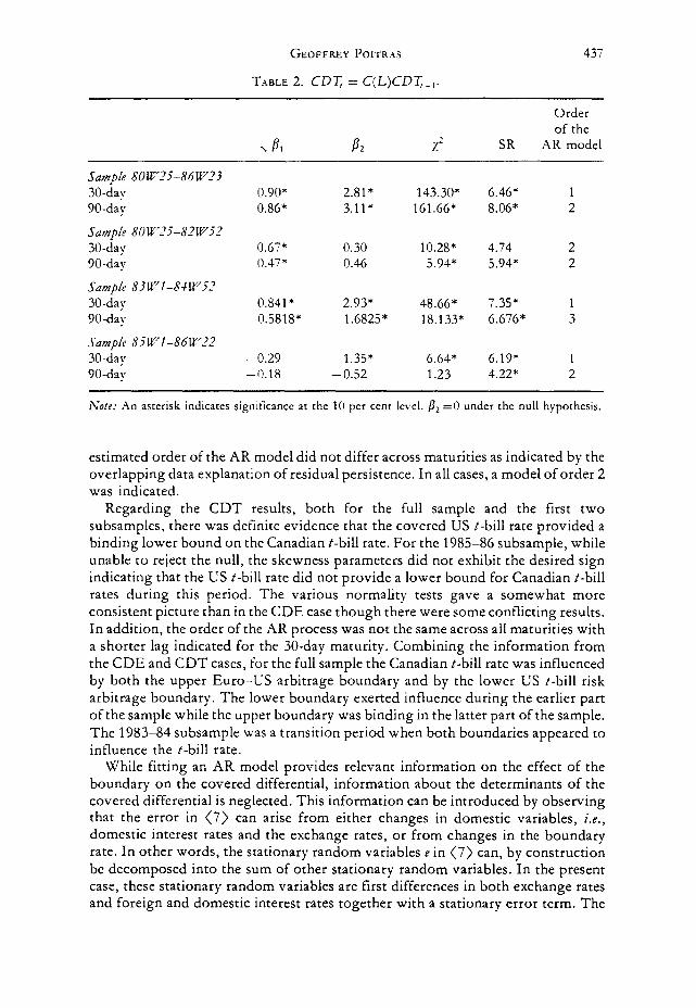
where: CD is the covered differential (either CDT or CDE), e is the white noise residual and A(L) is the backward lag operator where A(L) =a0 +a, L +a,.!_.’ +. . . and tin! =x,_, . The order of the AR process is determined by, initially, over-fitting an AR model. The lag structure is then pared by using likelihood ratio criteria to test the nested hypothesis that the highest order AR coefficient is zero. When the approriate model is selected, residuals from that model are used to compute the distributional tests. As noted, for CDE the expected sign for skewness of the residuals will be negative and residual skewness is expected to be positive for the CDT regressions. (For skewness, the expected sign for CDT is positive because the covered US t-bill provides a lower bound on the Canadian t-bill rate.) Distributional tests for the residuals from these regressions are given in Tables 1 and 2 respectively.

Table 1 reveals considerable support for the hypothesis that the upper arbitrage bound on CDE was binding for the full sample and the two later subsamples. For these periods, the skewness parameters are significant and have the expected sign. Only for the 1980-82 subsample case can the null hypothesis of normal skewness be accepted. Regarding normality of the residuals, results for both the omnibus tests and kurtosis were more mixed. For example, in two cases the SR test was unable to reject the null hypothesis of normally distributed residuals when the other three tests were able to reject the null. In two other cases, the SR rejected the null while the other tests were generally unable to reject. Somewhat surprisingly, the

GEOFFREY Porr~as 437

T.IBLE 2. CD?; = C(L)CD?;_,.

B, z2 SR

Order

of the

AR model

Sample 80 W-35-86 W23

30-day 90-day

Sample 80 W-77-82 WY-Z

30-day 90-day

Sample 83 W l-8-C Wi?

30-day 90-day

Sample 8iWl-86W22

30-day 90-day

0.90” 2.81*

0.86* 3.11*

0.67* 0.30 0.47* 0.46

0.841*

0.5818*

-0.29 1.35* -0.18 - 0.52

2.93*

1.6825*

143.30*

161.66*

10.28*

5.94*

48.66*

18.133*

6.64*

1.23

6.46*

8.06*

4.74 5.94*

7.35* 6.676*

6.19*

4.22*

1 2

2

2

1

3

I 2

iVote: An asterisk indicates significance at the 10 per cent level. bz =O under the null hypothesis.

estimated order of the AR model did not differ across maturities as indicated by the overlapping data explanation of residual persistence. In all cases, a model of order 2 was indicated.

Regarding the CDT results, both for the full sample and the first two subsamples, there was definite evidence that the covered US t-bill rate provided a binding lower bound on the Canadian t-bill rate. For the 1985-86 subsample, while unable to reject the null, the skewness parameters did not exhibit the desired sign indicating that the US t-bill rate did not provide a lower bound for Canadian t-bill rates during this period. The various normality tests gave a somewhat more consistent picture than in the CDE case though there were some conflicting results. In addition, the order of the AR process was not the same across all maturities with a shorter lag indicated for the 30-day maturity. Combining the information from the CDE and CDT cases, for the full sample the Canadian t-bill rate was influenced by both the upper Euro-US arbitrage boundary and by the lower US t-bill risk arbitrage boundary. The lower boundary exerted influence during the earlier part ofthe sample while the upper boundary was binding in the latter part of the sample.

The 1983-84 subsample was a transition period when both boundaries appeared to influence the t-bill rate.

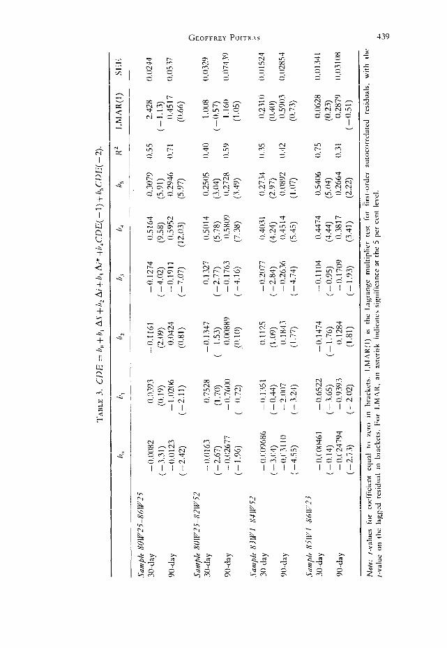
While fitting an AR model provides relevant information on the effect of the boundary on the covered differential, information about the determinants of the covered differential is neglected. This information can be introduced by observing that the error in (7) can arise from either changes in domestic variables, i.e., domestic interest rates and the eschange rates, or from changes in the boundary rate. In other words, the stationary random variables e in (7) can, by construction be decomposed into the sum of other stationary random variables. In the present case, these stationary random variables are first differences in both exchange rates and foreign and domestic interest rates together with a stationary error term. The

438 .Arbitragr Boundaries, Treasury Bills, and Corwrd lntrrrrt Parig

resulting regression equation is:*”

(8) CD = b,, +b,(S-S(-l))+b(i-i(-l))+bj(i*--*(-I))

+ G(L)CD( - 1) +J,

where: G(L) is a polynomial lag operator, J is the residual, i and i* have not been annualized, i.e., i and i* reflect the actual return on the trade and S is the spot eschange rate. Estimation of (8) aids in identifying the factors which ‘drive’ the

covered differential. However, the theoretical implications regarding the third and fourth moments of I are less clear. The presence of the boundary rate in the regression together with other variables which are known to be asymmetric over certain parts of the sample implies that a certain amount of skewness reduction can

be expected. Turning to the estimation results for (8) (reported in Tables 3 and 4), u-e see that

overall the most significant variable was the change in the boundary_ the ‘foreign’ interest rates. For both the Euro-US rate in the CDE regressions and the US t-bill rate for the CDT case the estimated coefficients for the change in foreign interest rates were highly significant and negative. These results indicate that changes in foreign interest rates have a much stronger influence on the size of the covered differential than do changes in domestic Canadian interest rates or the exchange rate. Evidence on the change in the spot exchange rate was mixed though the relevant coefficients were generally negative and significant in the later samples for both the CDE and CDT regressions. For both boundaries, the expected coefficient sign for exchange rate changes depends on the hypothesized reactions of market participants. If decreasing exchange rates induce traders to short the currency, then the forward-spot differential will fall, increasing the covered differential, and conversely for increasing eschange rates. This esplanation is consistent with the observed negative relationship between the covered differential and the change in

exchange rates. The other fundamental variable examined was the change in domestic interest

rates. For the CDT regressions, the Canadian t-bill rate was generally positive, as expected, though not usually significant. However, for the CDE regressions the change in the Canadian t-bill rate exhibited some unusual sign behavior. i.e., some negative, though generally insignificant, coefficients were observed for the 30-day case with all coefficients positive for the go-day case. Overall, these results for both the Canadian t-bill rate and the change in exchange rates may arise due to a feedback effect from policy intervention aimed at stabilizing conditions in the domestic money market or the foreign exchange market. Finally, for the CDE case, the order of the lagged endogenous variables carried over exactly from the previous AR estimations. For the CDT case, the order was much the same with a one-lag increase for the full sample and first subsample for the go-day maturity and the last subsample for the 30-day maturity.

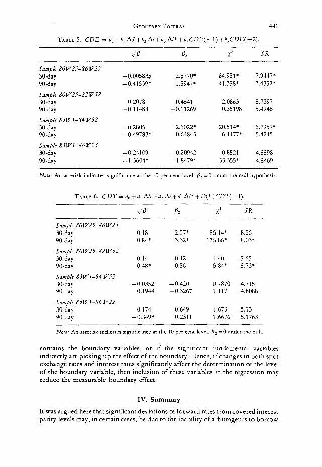
Turning to the distributional tests, the results reported in Tables 5 and 6 show that the addition of fundamental variables tends to reduce the estimated effect of the boundary on the covered differentials. This was particularly noticeable in the subsample estimates for CDT. For CDE, while there was a noticeable effect on skewness estimates for the 30-day case, the go-day results continued to support the boundary hypothesis, Although the theoretical implications are unknown, there are a number of possible interpretations for these results. For example, these results may not be incompatible with the boundary behavior hypothesis if the X matrix

GEOFFREY PorrR.ij

‘rnw

c 4.

C

/I7

=

c/,, +

</,

A.\

‘+,/,

A

i+d,

A

i* +

/~

(/~

)C/>

T(

- 1)

.

4,

4 4

4 O

rder

of

D

( I,

) R

2 L

MA

R(l

) Sl

ili

Sum

p/e

X0

WZ

5-X

(i

WZ

5

30.d

ay

90-d

ay

Sam

ple

X0

W25

-X2

W5-

7

30-d

ay

90-d

ay

0.01

4 0.

9694

0.

3210

(3

.28)

(2

.76)

(3

.40)

0.01

98

0.12

88

- 0.

076

1 (2

.53)

(0

.20)

(

- 0.

44)

0.02

79

2.39

66

0.28

05

(2.1

5)

(3.2

8)

(1.9

3)

0.06

78

0.80

7 0.

0954

(2

.78)

(0

.57)

(0

.337

)

Sam

ple

X3W

l-X

IW52

30

-day

90-d

ay

Sam

ple

X5

W l

-X6

W2J

30-d

ay

90.d

ay

0.02

1

(3.8

8)

0.03

456

(3.6

1)

0.00

2891

(0

.61)

-

0.02

565

( -

2.29

)

0.64

30

0.00

79

- 0.

7908

(1

.55)

(0

.05)

(

- 11

.34)

-2

.03x

0.

6181

-0

.408

6 (-

2.37

) (4

.32)

(

- 4.

75)

-0.3

583

0.02

650

-0.8

106

( -

1.38

) (0

.21)

(-

9.76

) -

1.22

9 0.

1278

-

0.05

706

(-2.

36)

(1.6

1)

( -

0.46

)

- 0.

6342

(

- 13

.80)

-0

.306

5 (

- 3.

89)

-0.6

122

( -

8.62

) -0

.344

5 (

- 2.

84)

1 0.

75

3 0.

80

2 0.

62

3 0.

71

1 0.

68

2 0.

75

2 0.

71

2 0.

51

1.00

9 (

- 1 .

OO

) 3.

059

(1.7

4)

3.21

1 (1

.76)

0.

512

(0.7

6)

1.90

1 (1

.36)

1.

1402

(-

0.10

)

1.67

3 (

- 1.

24)

0.53

62

(0.6

77)

0.04

24

0.07

68

0.05

60

0.10

70

See

Not

es

to T

able

3.

GEOFFREY POITRAS 441

TABLE 5. CDE = b,+b, AS+bz Ai+b, Ai*+b,CDE(-l)+bjCDE(-2).

V’P, 82 x2 SR

Sample 80 W25-86 W23 30-day 90-day

Sample 80 W25-82 W5.2 30-day 90-day

Sample 83 W l-84 W52 30-day 90-day

Sample 85Wl-86W23 30-day 90-day

-0.005835 2.5770* 84.951* 7.9447* -0.41539* 1.5947* 41.358* 7.4352*

0.2078 0.4641 2.0863 5.7397 -0.11488 -0.11269 0.35198 5.4946

-0.2805 2.1022* 20.514* 6.7957% - 0.49783+ 0.64843 6.1177* 5.4245

-0.24109 - 0.20942 0.8521 4.5598 -1.3604* 1.8479* 33.355* 4.8469

Note: An asterisk indicates significance at the 10 per cent level. & =0 under the null hypothesis.

TABLE 6. CDT = d,,+d, AS+d2 Ai+d,Ai*+D(L)CDT(-1).

\’ ‘PI I2 SR

Sample 80 W25-86 W-33 30-day 90-day

Sample 80 W25-82 WY2 30-day 90-day

Sample 83 WI-84 WJ-? 30-day 90-day

Sample 85W I-86W22 30-day 90-day

0.18 2.57” 86.14* 8.56 0.84* 3.32* 176.86* 8.03*

0.14 0.42 1.40 5.65 0.48* 0.56 6.84* 5.731

- 0.0352 - 0.420 0.7870 4.715 0.1944 -0.3267 1.117 4.8088

0.174 0.649 1.673 5.13 -0.349* 0.2311 1.6676 5.1763

Note: An asterisk indicates significance at the 10 per cent level. fi2 =O under the null.

contains the boundary variables, or if the significant fundamental variables indirectly are picking up the effect of the boundary. Hence, if changes in both spot exchange rates and interest rates significantly affect the determination of the level of the boundary variable, then inclusion of these variables in the regression may reduce the measurable boundary effect.

IV. Summary

It was argued here that significant deviations of forward rates from covered interest parity levels may, in certain cases, be due to the inability of arbitrageurs to borrow

442 .-lrbitrqgr Boundaries, Treasury Bills, and Cowrrd Intrrcst Parity

at one or both of the relevant interest rates. In the case of Canadian t-bills and Euro-US dollar deposits, arbitrageurs are able to borrow at the Euro-US rate but not at the Canadian t-bill rate. As a result, the covered Euro-US rate only provides an upper arbitrage boundary on Canadian t-bill rates. Similarly, for Canadian t-bills and US t-bills, arbitrageurs are not able to borrow at either rate. Hence, the lower boundary on Canadian t-bill rates provided by the covered US t-bill rate is only maintained through risk arbitrage based on the differential characteristics of US and Canadian t-bills. The covered differentials from the lower boundary were found to be larger and more volatile than for the upper boundary.

An adaptation of the methodology for estimating frontier functions was used to specify tests for the presence of boundary behavior. The resulting empirical work produced a number of useful conclusions. Examining the distributional properties

of regression residuals from an AR model for the covered differentials provided evidence that the covered Euro-US rate was an effective upper bound for the Canadian t-bill rate for the latter part of the sample. There was also evidence of a binding, lower bound provided by the covered US t-bill rate for the earlier part of the sample. VC’hen the set of regressors was espanded to include changes in foreign interest rates, domestic interest rates and eschange rates, changes in foreign interest rates were observed to have the most significant effect in determining the covered differentials.

1.

2.

3.

4.

5.

Notes

An example of how to design speculative trades based on boundary behaviour can be found in

Poitras (1987).

‘Domestic direct terms’ is defined as units of domestic currency to units of foreign currency, f.g.,

for Canadian investors this would be $C/$US. Regarding the use of forward contracrs in defining

CIP, much of the literature on CIP assumes that forward contracts are the relevant instrument for

evaluating CIP even though most ‘forward’ trading in currencies is done through su-ap trades. As

Clinton (1988) shows, this distinction has important implications for evaluating the transactions

cost boundaries for a CIP-based arbitrage. i\s a result, throughout the following the rerm

‘forward’ is used in the loose sense to include all methods of contracting for ‘future’ sale or

delivery of foreign exchange, i.e., forwards, swaps, options and futures.

.\mong the reasons why (l> and (2) may not be exact are clearing lags and holidays. Some care

should be taken to note that (1) and (2) e\ ress CIP on an unnualipd basis. When evaluating a :p

trade for a shorter period oftime it is necessary to correct the formulae to get the appropriate basis

points to be gained from doing the trade.

Specifically, for US investors US t-bills are exempt from stare and local tax while, depending on

the type of investor, Canadian t-bills may not be. In addition, the US t-bill market is substantially

more liquid than the Canadian t-bill market.

In the following, the occasional opportunities to use fixed to floating interest rate swaps to secure

sub-t-bill and/or sub-LIBOR financing are ignored. In addition, while it is implied that the

arbitrage is from Euros into t-bills, the arbitrage may actually be between Euros and other

domestic money market instruments, such as bankers acceptances or commercial paper.

However, insofar as the rates on other money market instruments are tied to rares on t-bills, funds

flows associated with arbitrages into other money market instruments will also affect t-bill rates.

6. Currently, about 70 per cent of available funds in the marker are denominated in US dollars.

Arguably, given the close connection between Euro-rates, the Euro-Canadian deposit rate could

be used as the upper boundary-allowing the boundary to be defined without reference to

currency of denomination. However, because the Euro-Canadian market is not deep, sizeable arbitrages would have to be done using the Euro-US market. In addition, Euro-Canadian

deposits made by Canadian residents with Canadian banks are subject to resen-e (and deposit

insurance) requirements while Euro-US deposits are not. Hence, use of the Euro-Canadian rate

would complicate the analysis because, not only would the arbitrage between the Euro-markets

GEOFFREY POITR.IS 443

and the Canadian t-bill market have to be esplained, fluctuations in the relationship between the

Euro-Canadian and Euro-US rate would have to be addressed.

7. Kreicher (1982) shows that institutional factors such as resetve requirements and deposit

insurance costs may affect the rate determination processes in the Euro and domestic markets. As

a result, appropriate adjustments have to be made to domestic rates before examining the

arbitrage relationship. These institutional factors are not as important in the Canadian case

because of the limited institutional restriction on Canadian banks operating in the Euro-US

markets (though foreign banks arbitraging the Euro-US/Canadian t-bill differential will be

subject to the requirements imposed by their country of origin).

8. To derive Figure 2, equation (4) is used with if being the US t-bill rate and the weak inequality

reversed.

9. This analysis assumes that the credit risk of the borrowing country is less than that of borrowers

issuing liabilities in the Euro-markets.

10. A number of different specifications of the frontier hypothesis are available (e.g., Forsund et al.,

1980). The most fundamental distinction is whether the frontier is stochastic or non-stochastic. If

the frontier is stochastic, then the estimated equation can, randomly, take values beyond the

frontier. If the frontier is non-stochastic, then the estimated equation is strictly bounded. This

puts a strong one-sided restriction on the residuals. For present purposes, the frontier is assumed

to be stochastic.

11. With some exceptions, previous empirical work provides support for null hypothesis of

symmetry in the underlying error distributions foor financial variables. This support increases as

the sampling frequency is increased, e.g., monthly data are generally mote symmetric than daily

data. For example, for first differences in rveeL~ foreign exchange rates, Westerfield (19--), Islam

(1982), and, to a lesser extent, Boothe and Glassman (1987) all present evidence in favour of

symmetry. Examining the distributions for the forward and spot eschange rates and Canadian

and US interest rate data used in this study, for the latter half of the sample the null hypothesis of

symmetry could not be rejected. However, the earlier parts of the sample exhibited a considerable

amount of skewness, arising primarily ftom a small number of outliers associated uith the

substantial moves in the market during that time period.

12. The estimations in Section III report results for a number of distributional tests: the standardized

sample moments of skewness (, K) and kurtosis (Pz) as well as two ‘omnibus’ tests: the

studentized range (SR) and an asymptotic chi-squared test combining the third and fourth sample

moments. The omnibus test is based on the asymptotic normality of the distributions for, BTand

P2. i.e., chi+quared(2)= T((b,)/6+(/$)‘;24), where T is the number of observations in the

sample. Because the small sample distributions for skewness and kurtosis are not independent,

corrected critical values provided by Bera and Alackenzie (1986) have been used.

To test for the autoregressive properties of the residuals, the Lagrange 5lultiplier (LSI) test for

(first-order) autocorrelated residuals has been calculated. The Lb1 test is based on the regression:

I;, = ,A%+nj,_, fl’,

where; is the regression residual, ,Y is the matrix of independent variables included in the original

regression, It is the coefficient vector associated with the A’ variables, t is the coefficient on the

lagged residual, and I is the equation error term. Also reported is the t-value on the coefficient of

the lagged residual -Durbin’s suggested alternative test when the Durbin h-test is inconclusive.

13. For 30- and 90-day t-bills, the data used are the weekly Wednesday Toronto/New York closing

quotes. Closing is defined as 4:30 EST/EDT. The actual maturity of the r-bills examined differs

slightly from the maturities stated because there is only one t-bill issued per week (in the case of

Canadian I-bills, usually maturing on a Friday), cd., on Wednesday the 90-day Canadian t-bill is

usually an 86day t-bill. For the Eurorates, London closing (noon EST/EDT) quotes are used.

Regarding exchange rate quotes, Toronto/New York forward and spot exchange rate closing

quotes are used 14. Based on the discussion in Section I, there should not be anv instances where the Euro-US rate

exceeds the covered Canadian rate. Those instances where Figure 1 indicates penetration of the

boundary resulted from two factors: different timing for the variables involved (i.e., the Euro quotes are taken at noon EST while all other quotes are 4:30) and policy intervention. Typically,

the difference in timing of the quotes will not significantly affect the covered differentials.

However, in the early part of the sample, there were a small number of instances when interest

rates and exchange rates moved substantially between the London close and the New York close.

444 Arbitrage Boundaries, Treasq Billr, and Covered Interest Parity

15.

16.

17.

18.

The one case where rates did not move coincided with central bank intervention ‘leaning against’

previous rate changes, actions which perpetuated the arbitrage opportunities.

There are central limit theorems relating to m-dependent random variables which apply here.

Subject to conventional regularity conditions, m-dependent random variables will be

asymptotically, normally distributed.

Because the theoretical moving average process for the errors implied by the overlapping data

problem is of high order, there is not much loss in precision from fitting a pure AR model to the

covered differentials. While it is possible to fit a more parsimonious ARMA model, the gains

from parsimony are offset by the considerable gain in expediency from fitting an AR model.

Switching to monthly and quarterly data to correct for the overlapping presents a degrees of

freedom problem, especially for the subsample estimates.

The relationship between A(L) and the MA error process can be derived by observing that in

MA form CD, =B*(L)e, =(I-B(L))e,. Inverting the polynomial operator gives

(I-B(L))-‘CD,=(I-A*(L))CD,=e,. Letting A*(L)=A(L)L and subtracting gives (7).

Hence, there is a (non-linear) relationship between the coefficients for the MA process and the AR

process.

Attempts to use more complicated forward and backward lag structures for the fundamental

variables in (8) were not successful. Among other things, this implies that CDE and CDT are not practical leading indicators of changes in i, i*, or S.

References

AIGNER, D., C. LOVELL, AND P. SCHMIDT, ‘Formulation and Estimation of Stochastic Frontier

Production Function Models,’ Journal of Econometrics, July 1977, 6: 21-37.

BAHMASI-OSKOOEE, M., AND S. DAS, ‘Transactions Costs and the Interest Parity Theorem,‘Journalof

Political Economy, August 1985, 93: 749-799. BELA, A., AND C. MCKENZIE, ‘Tests for Normality with Stable Alternatives,’ Journal of Statistical

Computation and Simulation, March 1986, 25: 37-52.

BOOTHE, P., AND D. GLASSMAN, ‘The Statistical Distribution of Exchange Rates: Empirical Evidence

and Economic Implications,’ Journaf of International Economics, May 1987, 22: 297-319.

BRANSON, W., ‘The Minimum Covered Differential Needed for International Arbitrage Activity,’

Journal of Politica/ Economy, November 1969, 77: 1028-1035.

CLINTON, K., ‘Transactions Costs and Covered Interest Parity,’ Journal of Pohical Economy, April

1988, 96: 358-370.

Cox, D., AND H. MILLER, The Theo9 of Stochastic Proterser, London: Chapman and Hall, 1965.

DEARDORFF, A., ‘One-Way Arbitrage and Its Implications for the Foreign Exchange Market,‘JournaI of Political Economy, April 1979, 87: 351-364.

DOOLEY, Xl., AND P. ISARD, ‘Capital Controls, Political Risk and Deviations From Interest-Rate Parity,’ Journaf of Political Economy, April 1980, 88: 370-384.

FORSUND, F., C. LOVELL, AND P. SCHMIDT, ‘A Survey of Frontier Production Functions,’ JournaI of Econometrics, May 1980, 13: 5-26.

FFZNKEL, J.. AND R. LEVICH, ‘Covered Interest Arbitrage: Unexploited Profits,’ Journal of Political Economy, April 1975, 83: 325-338.

FRENKEL, J., AND R. LEVICH, ‘Transactions Costs and Interest Arbitrage: Tranquil versus Turbulent

Periods,’ Jourmaf of Political Eronomy, December 1977, 85: 1209-1266.

FRENKEL, J., AND R. LEVICH, ‘Covered Interest Arbitrage in the 1970’s,’ Economic Letterr, March 1981, 8: 267-274.

GRUBEL, H., Forward Exchange, Speculation and the International Flow of Capital, Stanford: Stanford University Press, 1966.

HANSEN, L., AND R. HODRICK, ‘Forward Exchange Rates as Optimal Predictors of Future Spot

Exchange Rates,’ Journal of Politica/ Economy, October 1980, 88: 829-853.

HUSTED, S., AND J. KITCHEN, ‘Some Evidence of the International Transmission of US Xioney

Supply Announcements,’ Journal of Money, Credit and Banking, November 1985, 17: 456-466. ISLAM, S., ‘Statistical Distribution of Short-Term Exchange Rate Variations,’ Federal Reserve Bank

of New York, Research Paper No. 8215, April 1982.

JOHNSOS, N., AND Korz, S., Continuous Univariate Distributions--2, New York: Houghton Mifflin, 1970.

. GEOFFREY POITRAS 445

JUDGE, G., W. GRIFFITHS, R. HILL, H. LUTKEPOHL, &VD T.-C. LEE, The Theory and Practice of

Economics, New York: Wiley, 1985.

KNIGHT, J., ‘Non-Normal Errors and the Distribution of OLS and 2SLS Structural Estimators,’

Econometric Theory, April 1986, 2: 75-106.

KREICHER, L., ‘Eurodollar Arbitrage,’ Federal Reserve Bank of New YorkQuarter4 Rcvierv, Summer

1982: 10-21.

LONDON, A., ‘The Stability of the Interest Parity Relationship between Canada and the United States,’

Rev& of Economics and Statistics, November 1981, 63: 625-626.

MARSTON, R., ‘Interest Arbitrage in the Euro-Currency IMarkets, European Economic Review, January

1976, 7: 1-13.

OLSON, J., P. SCHMIDT, AND D. WALDSIAN, ‘A Monte Carlo Study of Estimators of Stochastic

Frontier Production Functions,’ JournaI of Econometrirs, May 1980, 13: 67-82.

OTANI, I., AND S. TIWARI, ‘Capital Controls and the Interest Parity Rate: The Japanese Experience,

1978-81,’ I.M.F. Staff Papers, December 1981, 28: 793-815.

OVERTURF, S., ‘Interest Rate Expectations and Interest Parity,’ Journal of International Money and Finance, March 1986, 5: 91-98.

PEARSON, E., R. D’AGOSTINO, AND K. BOWMAN, ‘Tests for Departures from Normality: Comparison

of Powers,’ Biometrika, 1977, 64: 231-246. PIPPENGER, J., ‘Interest Arbitrage Between Canada and the U.S.,’ Canadian Journalof Eronomirs, May

1978, 11: 183-193.

POITRAS, G., ‘Golden Turtle Tracks: In Search of Unexploited Profits in Gold Spreads,’ Journ& of

Futures Murkets, August 1987, 7: 397-412.

PRACHOWNY, M. F. J., ‘A Note on Interest Parity and the Supply of Arbitrage Funds,’ Journal of Political Economy, May/June 1970, 78: 540-545.

SHARE, I., ‘Interest Parity, Monetary Policy and the Volatility of Australian Short-Term Interest

Rates: 1978-82,’ Economic Rerotd, December 1985, 61: 436-444.

STOCKMAN, A., ‘Risk, Information and Foreign Exchange Rates, ’ in J. Frenkel and H. Johnson, eds,

The Economics of Exchange Rates, Reading, Mass.: Addison-Wesley, 1978, ch. 9.

WALDMAN, D.;‘A Stationary Point for the Stochastic Frontier Likelihood,’ Journal of Econometrics, February 1982, 18: 275-279.

WESTERFIELD, J., ‘An Examination of Foreign Exchange Risk Under Fixed and Floating Exchange

Rate Regimes,’ JonrnaL of Internation& Economics, May 1977, 7: 181-200.

WHITE, H., AND G. MACDONALD, ‘Some Large-Sample Tests for Nonnormalty in the Linear

Regression Model,’ Journal of the American Statistical Association, March 1980, 75: 16-27.