
Aquifer Test Cromwell - health.state.mn.us · Analysis of the Cromwell, Minnesota Well 4 (593593)...
75
Analysis of the Cromwell, Minnesota Well 4 (593593) Aquifer Test CONDUCTED ON MAY 24, 2017 CONFINED QUATERNARY GLACIAL-FLUVIAL SAND AQUIFER
Transcript of Aquifer Test Cromwell - health.state.mn.us · Analysis of the Cromwell, Minnesota Well 4 (593593)...

Analysis of the Cromwell, Minnesota Well 4 (593593) Aquifer Test CONDUCTED ON MAY 24, 2017 CONFINED QUATERNARY GLACIAL-FLUVIAL SAND AQUIFER
T E S T 2 6 1 2 , C R O M W E L L 4 ( 5 9 3 5 9 3 ) M A Y 2 4 , 2 0 1 7
2
Analysis of the Cromwell, Minnesota Well 4 (593593) Aquifer Test Conducted on May 24, 2017
Minnesota Department of Health, Source Water Protection Program PO Box 64975 St. Paul, MN 55164-0975 651-201-4700 [email protected] www.health.state.mn.us/divs/eh/water/swp
To obtain this information in a different format, call: 651-201-4700.
Upon request, this material will be made available in an alternative format such as large print, Braille or audio recording. Printed on recycled paper.

T E S T 2 6 1 2 , C R O M W E L L 4 ( 5 9 3 5 9 3 ) M A Y 2 4 , 2 0 1 7
3
Contents Analysis of the Cromwell, Minnesota–Well 4 (593593) Aquifer Test............................................. 1
..................................................................................................................................................... 1
Data Collection and Analysis ....................................................................................................... 7
Description .................................................................................................................................. 7
Purpose of Test ....................................................................................................................... 7
Well Inventory ......................................................................................................................... 7
Other Interfering Wells ........................................................................................................... 7
Test Setup ............................................................................................................................... 8
Weather Conditions ................................................................................................................ 8
Discharge Monitoring ............................................................................................................. 8
Data Collection ........................................................................................................................ 8
Qualitative Aquifer Hydraulic Response ..................................................................................... 9
Quantitative Analysis ................................................................................................................ 10
Transient-Horizontal Flow..................................................................................................... 11
Steady-State Horizontal Flow ............................................................................................... 11
Steady-State Vertical Flow .................................................................................................... 12
Steady-State Leakage Caused by Pumping ........................................................................... 12
Simultaneous Solution for Horizontal and Vertical Flow ...................................................... 13
Additional Analyses for Comparison to other Parts of the Dataset ..................................... 13
Conclusion ................................................................................................................................. 13
Acknowledgements ................................................................................................................... 14
References ................................................................................................................................ 14
Tables and Figures ........................................................................................................................ 16

T E S T 2 6 1 2 , C R O M W E L L 4 ( 5 9 3 5 9 3 ) M A Y 2 4 , 2 0 1 7
4
List of Tables Table 1. Summary of Results for Leaky Confined - Radial Porous Media Flow ............................ 16
Table 2. Aquifer Test Information ................................................................................................. 17
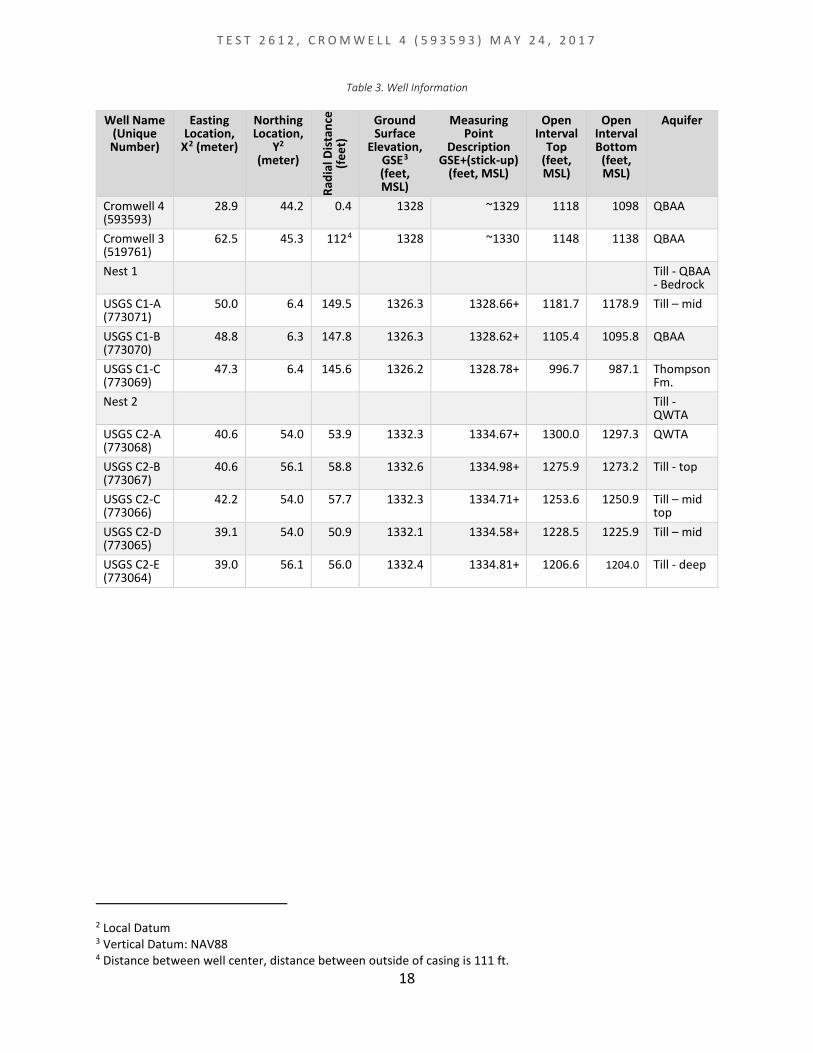
Table 3. Well Information ............................................................................................................. 18
Table 4. Data Collection ................................................................................................................ 19
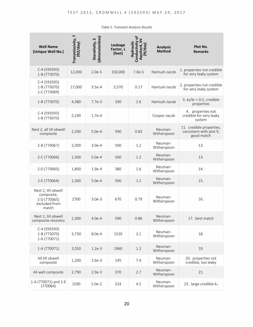
Table 5. Transient Analysis Results ............................................................................................... 20
Table 6. Steady-state Analysis Results .......................................................................................... 21
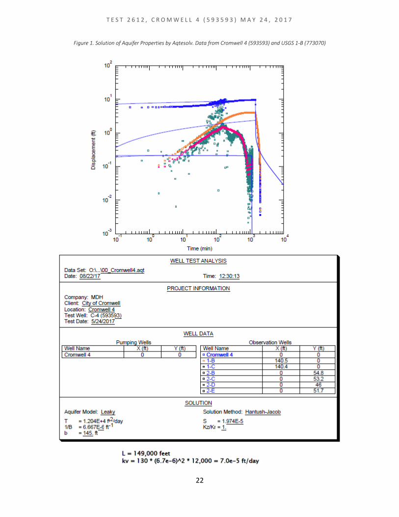
List of Figures Figure 1. Solution of Aquifer Properties by Aqtesolv. Data from Cromwell 4 (593593) and USGS 1-B (773070) .................................................................................................................................. 22
Figure 2. Solution of Aquifer Properties by Aqtesolv. Showing Data from Cromwell 4 (593593), USGS 1-B (773070) and USGS 1-C (773071) ................................................................................. 23
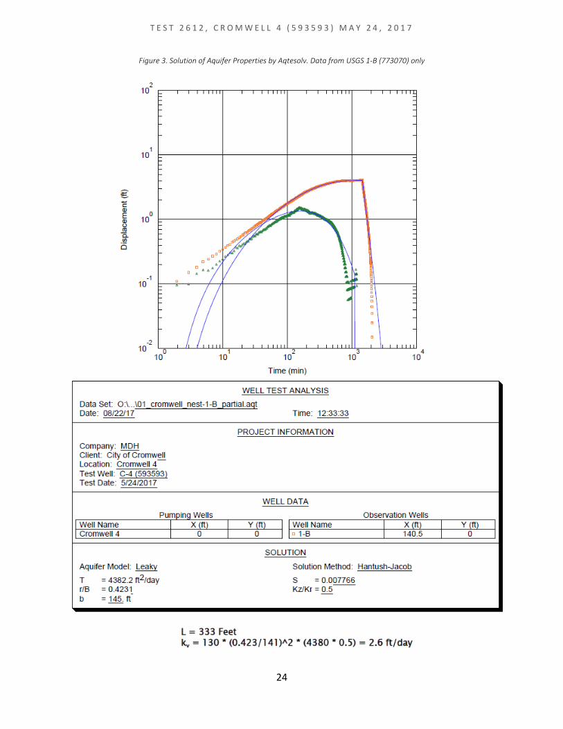
Figure 3. Solution of Aquifer Properties by Aqtesolv. Data from USGS 1-B (773070) only .......... 24
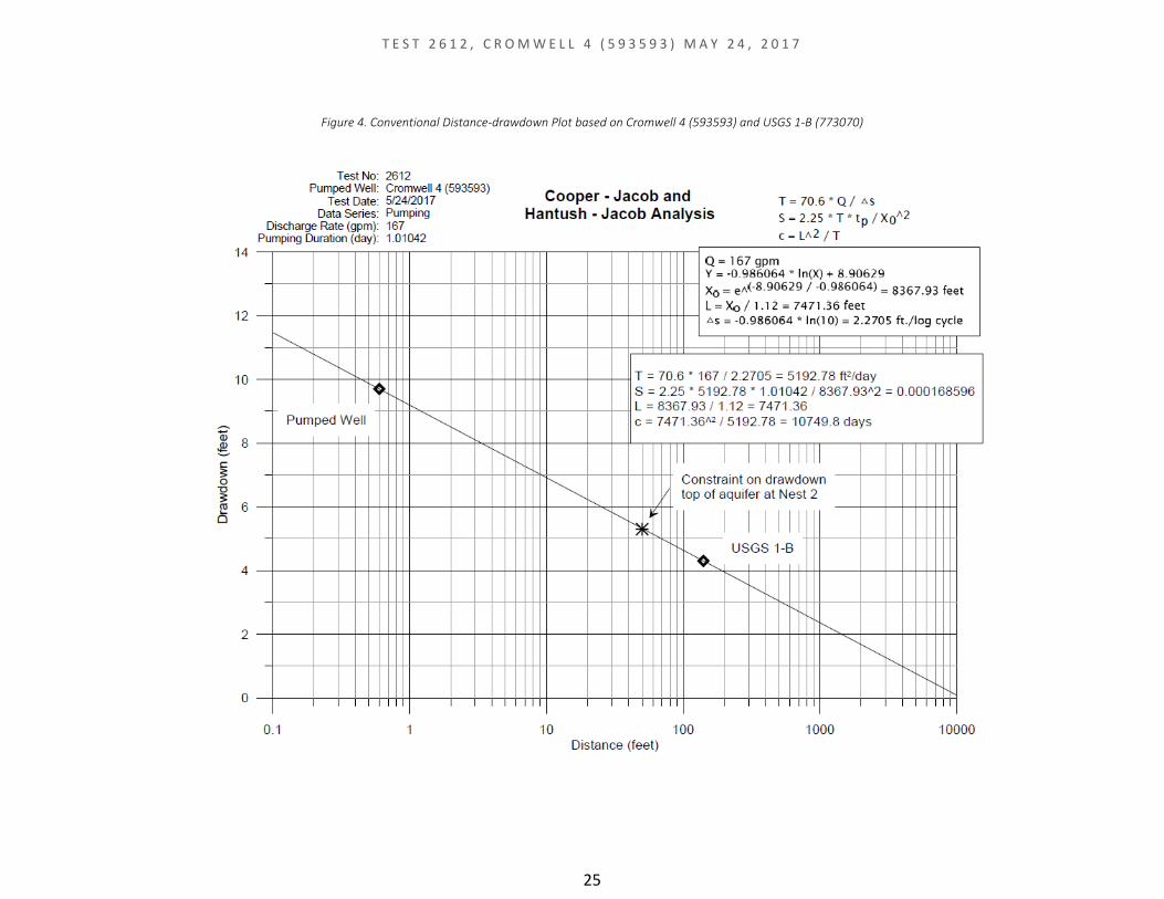
Figure 4. Conventional Distance-drawdown Plot based on Cromwell 4 (593593) and USGS 1-B (773070) ........................................................................................................................................ 25
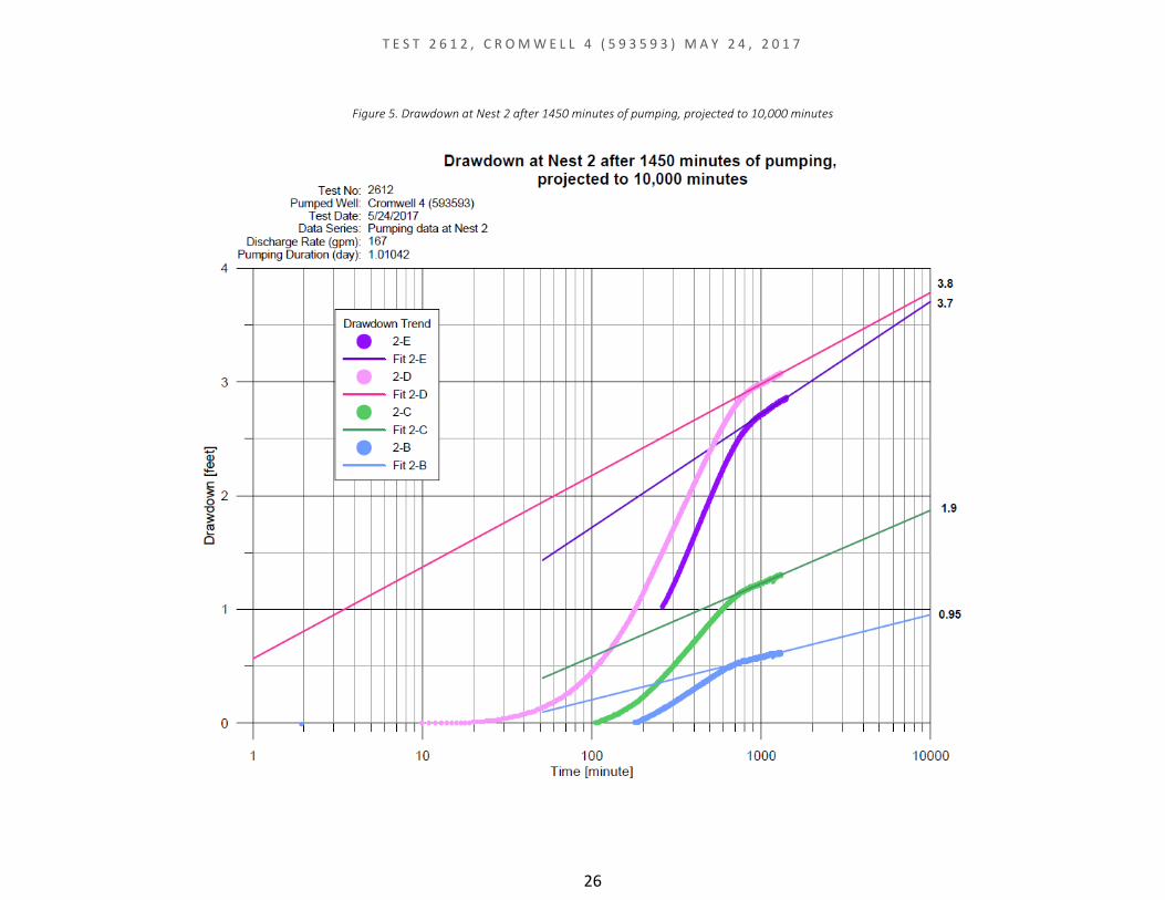
Figure 5. Drawdown at Nest 2 after 1450 minutes of pumping, projected to 10,000 minutes ... 26
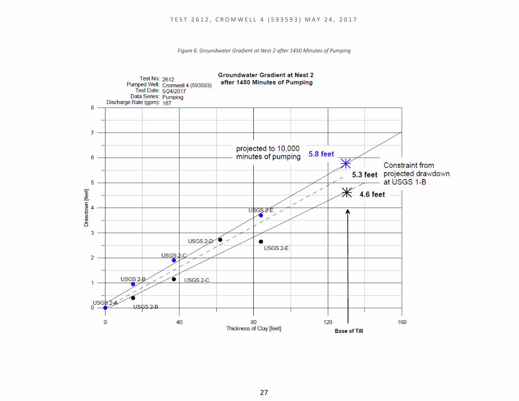
Figure 6. Groundwater Gradient at Nest 2 after 1450 Minutes of Pumping ............................... 27
Figure 7. Drawdown at Nest 1 after 1450 minutes of pumping, projected to 10,000 minutes ... 28
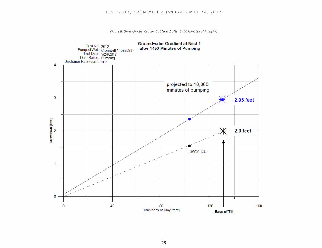
Figure 8. Groundwater Gradient at Nest 1 after 1450 Minutes of Pumping ............................... 29
Figure 9. Comparison of Drawdowns at 1450 Minutes of Pumping at Nests 1 and 2, at Nase of Till, to that in Aquifer .................................................................................................................... 30
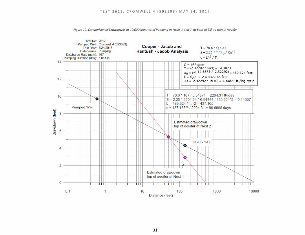
Figure 10. Comparison of Drawdowns at 10,000 Minutes of Pumping at Nests 1 and 2, at Base of Till, to that in Aquifer ................................................................................................................ 31
Figure 11. Solution of Aquifer Properties by Aqtesolv. Data from USGS 2-B, 2-C, 2-D, and 2-E .. 32
Figure 12. Solution of Aquifer Properties by Aqtesolv. Data from USGS 2-B only ....................... 33
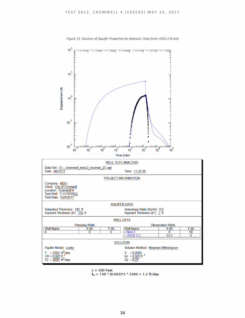
Figure 13. Solution of Aquifer Properties by Aqtesolv. Data from USGS 2-B only ....................... 34
Figure 14. Solution of Aquifer Properties by Aqtesolv. Data from USGS 2-C only ....................... 35
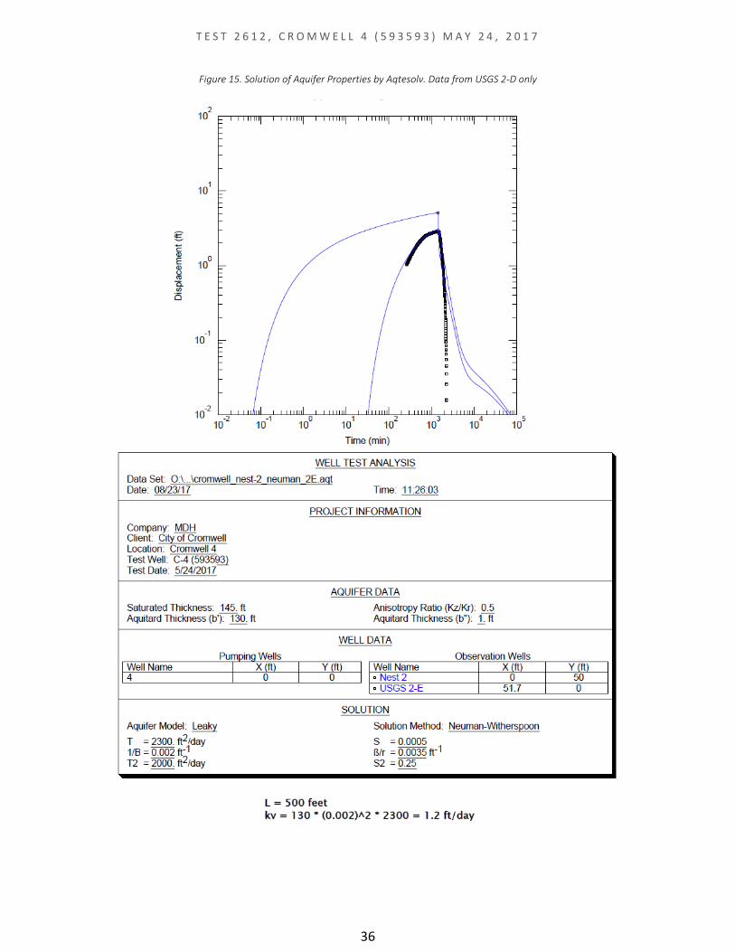
Figure 15. Solution of Aquifer Properties by Aqtesolv. Data from USGS 2-D only ....................... 36
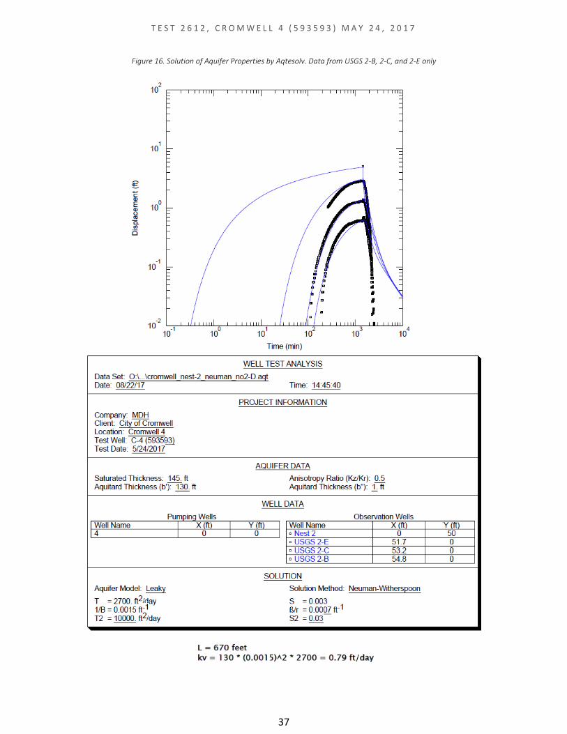
Figure 16. Solution of Aquifer Properties by Aqtesolv. Data from USGS 2-B, 2-C, and 2-E only .. 37
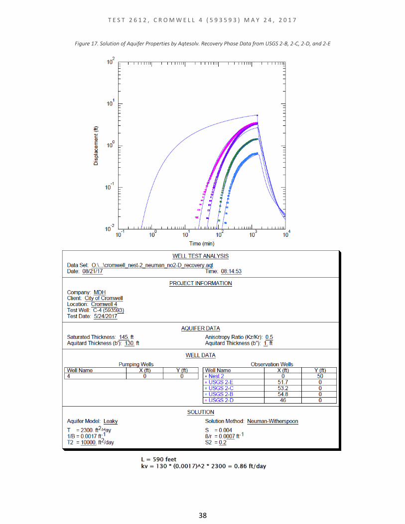
Figure 17. Solution of Aquifer Properties by Aqtesolv. Recovery Phase Data from USGS 2-B, 2-C, 2-D, and 2-E ................................................................................................................................... 38

T E S T 2 6 1 2 , C R O M W E L L 4 ( 5 9 3 5 9 3 ) M A Y 2 4 , 2 0 1 7
5
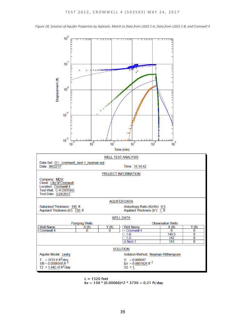
Figure 18. Solution of Aquifer Properties by Aqtesolv. Match to Data from USGS 1-A, Data from USGS 1-B, and Cromwell 4 ............................................................................................................ 39
Figure 19. Solution of Aquifer Properties by Aqtesolv. Match to Data from USGS 1-A and Modeled Drawdown at the Base of Till, Data from USGS 1-B, and Cromwell 4 ........................... 40
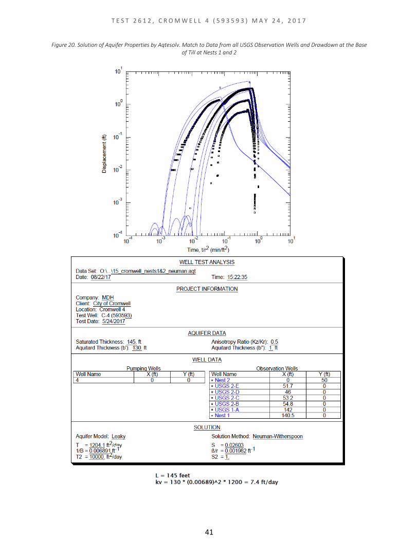
Figure 20. Solution of Aquifer Properties by Aqtesolv. Match to Data from all USGS Observation Wells and Drawdown at the Base of Till at Nests 1 and 2 ............................................................ 41
Figure 21. Solution of Aquifer Properties by Aqtesolv. Match to all data .................................... 42
Figure 22. Similarity in Slope of 1-A and 2-E ................................................................................. 43
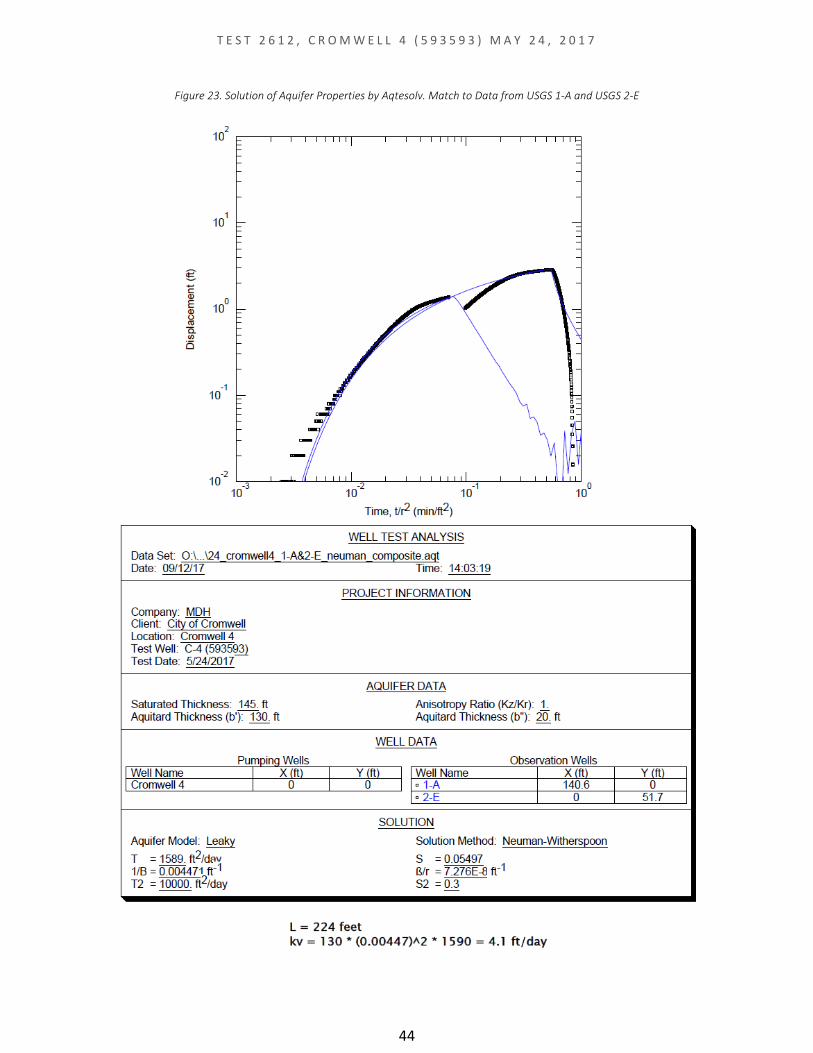
Figure 23. Solution of Aquifer Properties by Aqtesolv. Match to Data from USGS 1-A and USGS 2-E ................................................................................................................................................. 44
Figure 24. Agarwal Analysis .......................................................................................................... 45
Figure 25. Solution of Aquifer Properties by Aqtesolv. Analysis of Recovery Data from Pumped Well ............................................................................................................................................... 46
Figure 26. Well Identification ........................................................................................................ 47
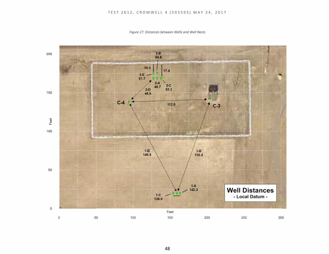
Figure 27. Distances between Wells and Well Nests .................................................................... 48
Figure 28. Schematic Section Across Site ..................................................................................... 49
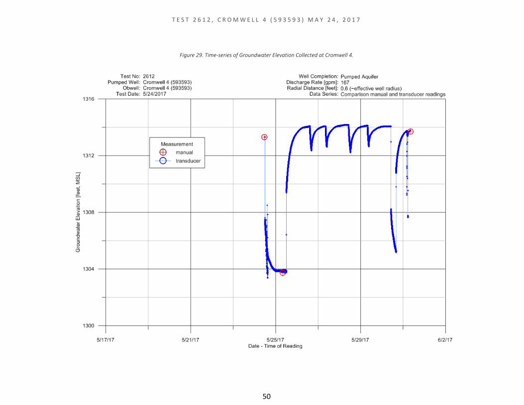
Figure 29. Time-series of Groundwater Elevation Collected at Cromwell 4. ............................... 50
Figure 30. Time-series of Groundwater Elevation Collected at USGS 1-A. .................................. 51
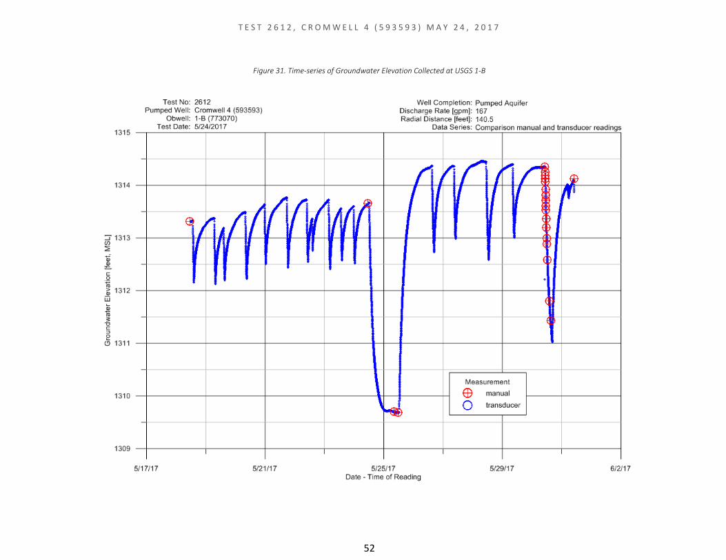
Figure 31. Time-series of Groundwater Elevation Collected at USGS 1-B .................................... 52
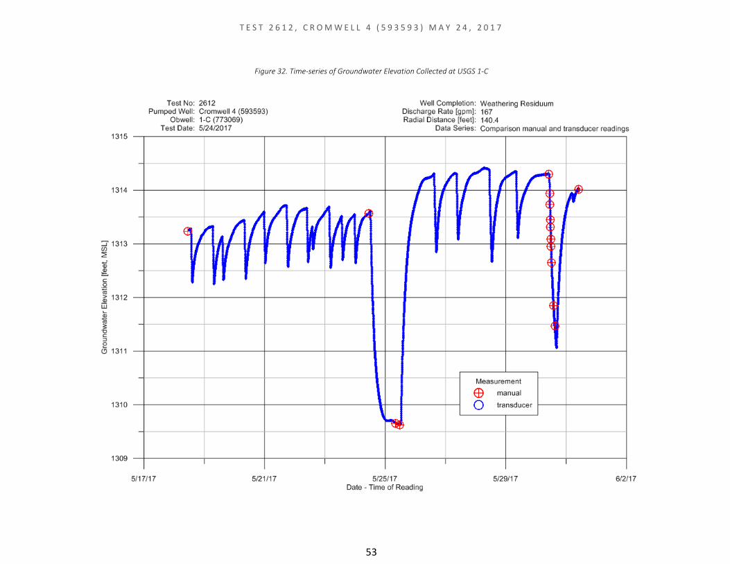
Figure 32. Time-series of Groundwater Elevation Collected at USGS 1-C .................................... 53
Figure 33. Time-series of Groundwater Elevation Collected at USGS 2-A ................................... 54
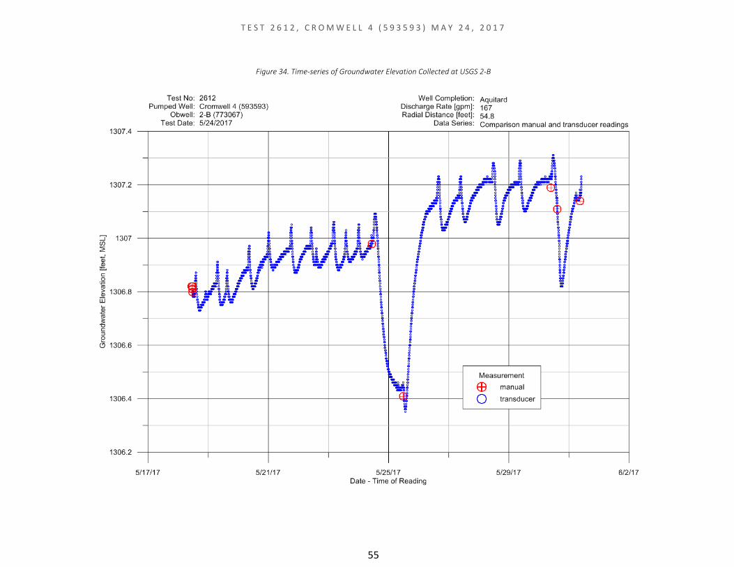
Figure 34. Time-series of Groundwater Elevation Collected at USGS 2-B .................................... 55
Figure 35. Time-series of Groundwater Elevation Collected at USGS 2-C .................................... 56
Figure 36. Time-series of Groundwater Elevation Collected at USGS 2-D ................................... 57
Figure 37. Time-series of Groundwater Elevation Collected at USGS 2-E .................................... 58
Figure 38. Time-series of Groundwater Elevation Collected at all Wells ..................................... 59
Figure 39. Time-series of Groundwater Elevation Collected at Cromwell 4 and Nest 1 .............. 60
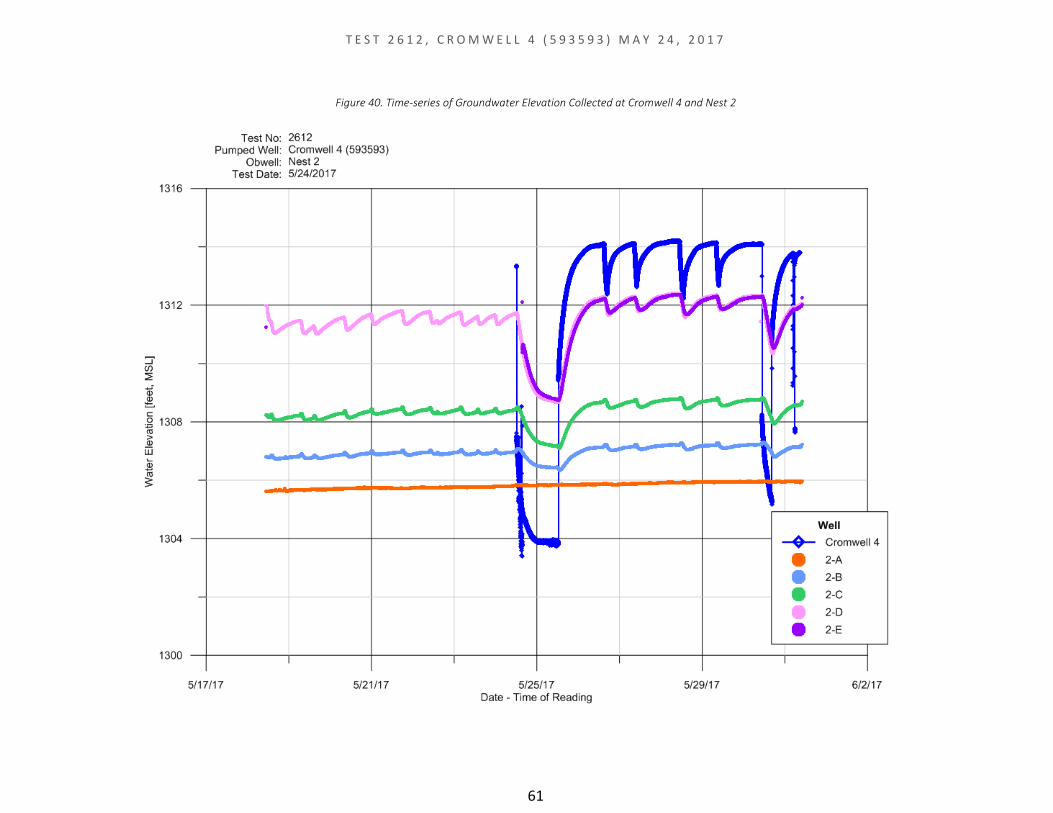
Figure 40. Time-series of Groundwater Elevation Collected at Cromwell 4 and Nest 2 .............. 61
Figure 41. Time-series of Groundwater Elevation Collected at USGS 2-A and Barometric Pressure as Difference in Water Level .......................................................................................... 62
Figure 42. Aqtesolv plot of diagnostic slope for spherical flow and data from USGS 1-B and 1-C....................................................................................................................................................... 63
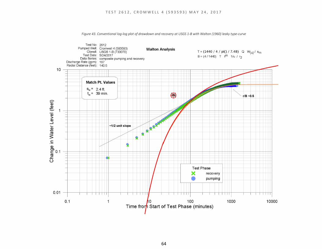
Figure 43. Conventional log-log plot of drawdown and recovery at USGS 1-B with Walton (1960) leaky type-curve ............................................................................................................................ 64
T E S T 2 6 1 2 , C R O M W E L L 4 ( 5 9 3 5 9 3 ) M A Y 2 4 , 2 0 1 7
6
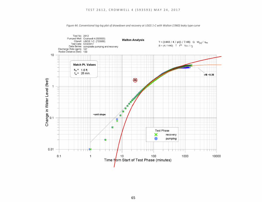
Figure 44. Conventional log-log plot of drawdown and recovery at USGS 1-C with Walton (1960) leaky type-curve ............................................................................................................................ 65
Figure 45. Well and Boring Report - Well 593593 ........................................................................ 66
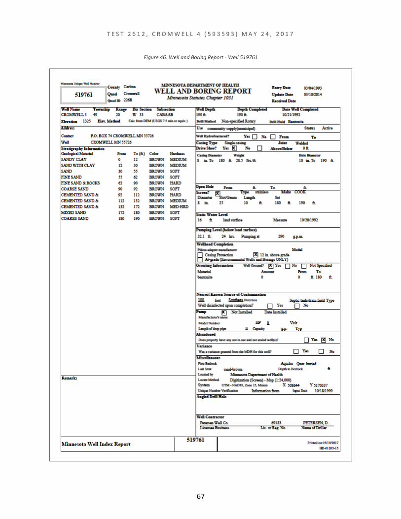
Figure 46. Well and Boring Report - Well 519761 ........................................................................ 67
Figure 47. Well and Boring Report - Well 773071 ........................................................................ 68
Figure 48. Well and Boring Report - Well 773070 ........................................................................ 69
Figure 49. Well and Boring Report - Well 773069 ........................................................................ 70
Figure 50. Well and Boring Report - Well 773068 ........................................................................ 71
Figure 51. Well and Boring Report - Well 773067 ........................................................................ 72
Figure 52. Well and Boring Report - Well 773066 ........................................................................ 73
Figure 53. Well and Boring Report - Well 773065 ........................................................................ 74
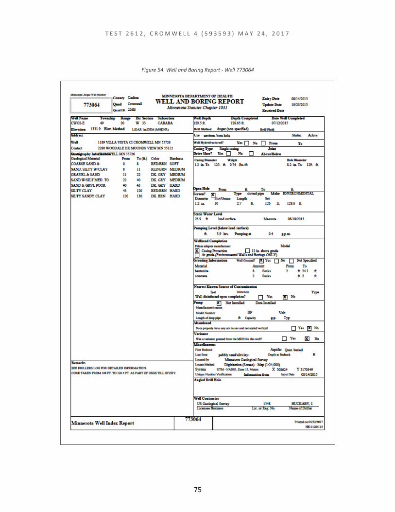
Figure 54. Well and Boring Report - Well 773064 ........................................................................ 75
T E S T 2 6 1 2 , C R O M W E L L 4 ( 5 9 3 5 9 3 ) M A Y 2 4 , 2 0 1 7
7
Data Collection and Analysis The constant-rate aquifer test performed at Cromwell 4 (593593) was conducted as described below. The test results are summarized in Table 1. The specifics of test location, scope, and timing are presented in Table 2, Table 3, and Table 4. Data were analyzed using standard methods cited in references. Individual analyses are presented the Figures 1-25 and are summarized in Table 5 and Table 6. Figures 26-44 include maps, comparison of manual and electronic data, and any other test documentation. Records of well construction are contained in Figures 45-54.
Description Purpose of Test The test of Cromwell 4 was conducted by the Minnesota Department of Health (MDH) Source Water Protection Unit as a small part of a longer-term project led by the United States Geological Survey (USGS). The overall purpose of the study is to assess the rates of groundwater recharge through low-conductivity glacial sediments at various sites in Minnesota.
Specific to Cromwell, eight observation wells were installed by the USGS in 2015. Water elevations were recorded on a one-hour interval in five of these wells for approximately one-year. The USGS had completed its data collection and was preparing to seal the observation wells. Prior to sealing the wells, notification was provided to the partner agencies relative to the completion of the work. At that time, staff in the Source Water Protection Unit recognized that this configuration of observation wells is nearly ideal for conducting a short-term constant-rate aquifer test that is designed to estimate vertical groundwater flow induced by pumping. Therefore prior to sealing the wells, MDH proposed to conduct tests that would complement the USGS data collection efforts.
Well Inventory The well records are presented in Figures 45-54 and the well construction is summarized in Table 2. Detailed site plans are shown in Figure 26 and Figure 27.
Hydrogeologic Setting These records were used to assess the hydrogeologic setting and identify the appropriate conceptual model for data analysis. A schematic section through the test site is shown on Figure 28 to illustrate the three layers that comprise the flow system; water table, aquitard, aquifer, and the construction of wells within these layers.
Other Interfering Wells No other high capacity wells exist in the area to cause interference.

T E S T 2 6 1 2 , C R O M W E L L 4 ( 5 9 3 5 9 3 ) M A Y 2 4 , 2 0 1 7
8
Test Setup The USGS provided the pressure transducers and data loggers used for long-term monitoring, re-programmed to a one-minute interval. MDH hydrologists, Tracy Lund and Justin Blum, traveled to Cromwell on May 18, 2017 to assess site conditions and re-install the transducers to collect background water level and barometric data. At that time, the flowmeter-totalizer had been removed for cleaning and calibration. Mr. Tom Johnson, the water operator, indicated that the flowmeter would be returned to service shortly and the test was tentatively scheduled to begin on May 23, 2017. Access to Cromwell 3 (519761) is restricted and the only means to measure the water level is via a bubbler-line. A transducer could be placed in Cromwell 4 to monitor water levels. A prior test of Cromwell 3 was conducted by the MDH in 2001. The location of the obwell nests relative to the PWS wells is slightly closer to Cromwell 4 than 3. The obwells constructed in the till are within 60 feet of Well 4 and are therefore more likely to respond to pumping. Because of these factors; access to the wells, prior tests, and the relative distance of the well nests, caused Cromwell 4 to be preferred for testing. After the flowmeter was reinstalled, MDH staff mobilized for the test on May 24, 2017, arriving on-site at 10:00. The flow monitoring equipment and pump controls were inspected with the operator. Discussions with the operator indicated that the system demand is much smaller than the capacity of the well and water will have to be wasted during the 24-hour pumping phase. He considered putting a discharge control on one of the hydrants to drain the excess but opted to let the tower fill and overflow to the established drain. This presented no flooding or erosion hazard and did not require monitoring for concerns of public safety.
An MDH pressure transducer was installed in Cromwell 4; programmed to a 20 second interval, and scheduled to begin data collection 5/24/2017 at 12:00. Static levels were collected from all accessible wells prior to beginning the test. A transducer (in-line with a compressor) was attached to the Cromwell Well 3 bubbler-line to attempt to collect water levels.
Weather Conditions Conditions were cool and rainy during background data collection. No appreciable precipitation occurred during pumping and recovery.
Discharge Monitoring The totalizing flow meter was read manually to document the pumping rate. The operator flushed hydrants between 12:30 and 15:00, early in the pumping phase, putting some of the excess water to productive use.
Data Collection The pump was started at 12:10:04 on 5/24/2017 by hand control. The compressor/transducer setup on Well 3 did not collect usable data. Water levels were collected manually from the accessible wells and data were downloaded to check the operation of the transducers.
It was found that the transducer in well USGS 2-E (773064) was set too deep in the well and did not collect usable data during background and early pumping. The submergence of the transducer was adjusted and a static collected at 15:30. Data collected after about 280

T E S T 2 6 1 2 , C R O M W E L L 4 ( 5 9 3 5 9 3 ) M A Y 2 4 , 2 0 1 7
9
minutes of pumping (~18:00 on 5/24/2017) are valid. The transducers in all other observation wells appeared to functioning properly.
In the morning of 5/25/2017 distances from the pumped well to the observation wells and other features visible on aerial photos were measured with fiberglass tape. Data were downloaded from the transducers prior to end of pumping/start of recovery. Recovery began at 12:25:00 5/25/2017.
During the recovery period, over the Memorial Day weekend, the water operator agreed to manipulate the pump controls is such a way that Well 4 would not be pumped and Well 3 would be used to meet demand. Normal operation is to alternate the wells, accomplished by an automatic switch in the pump controls. Bypass of the switch provided data from short-term pumping of Well 3 to compare to that from the test of Well 4, just completed, see test 2613.
Data were downloaded on 5/30/2017 and water levels measured. The recovery-phase data from USGS 1-A was lost during the download process. Also, inspection of the data from Well 4 showed that the hydrant flushing caused anomalous changes in water level in the early part of the pumping-phase. Because of these problems, it was decided to perform a second, short-term constant-rate test, of Well 4 to attempt to collect additional early-time data from the pumped well and USGS 1-A. This test was run the same way as the earlier constant-rate test but for an abbreviated pumping period (345 minutes) with an overnight recovery. The final water levels were measured on 5/31/2017 and the equipment removed from the wells. Results of this short-term test are described in a separate document, see test 2619.
Qualitative Aquifer Hydraulic Response Detailed site plans are shown in Figure 26 and Figure 27, identifying the wells and distances between the wells. A schematic cross section is provided for visual context of the test conditions, Figure 28. Comparison of manual and transducer data are shown Figure 29 through Figure 37. All but one well showed a response to pumping. USGS 2-A, constructed in the water table aquifer showed no response, as expected. The groundwater gradient is upward under ‘static conditions,’ including typical pumping to meet the system demand, Figure 38. The ambient difference in water elevation across the till at the well site is approximately 8.4 feet. Comparisons of water elevations between wells at the nests are shown on Figure 39 and Figure 40. From these comparisons, the more intensive pumping of this constant-rate test temporarily reversed the gradient within a short distance from the pumped well (~10 feet) and generated a strong signal for analysis of hydraulic properties.
The water elevations appear to trend upward over the data collection period. No appreciable change in water level can be attributed to changes in barometric pressure, Figure 41. The trend of the increase in water level shown on Figure 37was removed prior to analysis.
The only truly anomalous hydraulic responses were seen in wells USGS 2-B and 2-C, Figure 34 and Figure 35, respectively. These wells showed consistent, transient, reverse water level variation with the start of pumping of either Cromwell 3 or 4; conditions under which elevations would be expected to decrease. The reverse water variation also occurred at the end of the Cromwell 4 pumping phase. The magnitude of the response was about 0.1 foot and dissipated within about twenty minutes of the change in conditions. This phenomenon has been described in the literature as a poro-elastic response, Wolf (1970). Reverse water level fluctuations are characteristic of wells constructed in materials with a low conductivity and high elasticity (clay) that are in contact with materials of high conductivity and high compressive strength (sand). This condition is rarely observed and is the first time that it has been encountered (that we are aware of) in Minnesota. Because of this poro-elastic
T E S T 2 6 1 2 , C R O M W E L L 4 ( 5 9 3 5 9 3 ) M A Y 2 4 , 2 0 1 7
10
response, data from these wells are considered to be most representative of conditions within the till, relative to the response of other wells in this nest.
Within the aquifer itself, the simplifying assumptions of commonly used analysis techniques consider the movement of groundwater induced by pumping to be exclusively horizontal. In the case of this analysis, vertical head differences within the aquifer within 200 feet of the pumped well cannot be neglected. The pumping well is constructed with a twenty-foot screen, centered 55 feet below the top of the sand and gravel aquifer. The total thickness of the aquifer in this location is 145 feet. This type of well construction where the aquifer is screened over only a portion of the whole thickness is known as ‘partially penetrating.’ Because of this well construction, within small radial distances (tens of feet) from the pumped well, groundwater flow is spherical rather than horizontal; transitioning to horizontal with increasing radial distance. The rule of thumb (Hantush, 1964) for estimation of the radial distance at which this transition to horizontal flow is complete:
rh = 1.5 ∗ (𝑎𝑎𝑎𝑎𝑎𝑎𝑎𝑎𝑎𝑎𝑎𝑎𝑎𝑎 𝑡𝑡ℎ𝑎𝑎𝑖𝑖𝑖𝑖𝑖𝑖𝑎𝑎𝑖𝑖𝑖𝑖) ∗ (ℎ𝑜𝑜𝑜𝑜𝑜𝑜𝑜𝑜𝑜𝑜𝑜𝑜𝑜𝑜𝑜𝑜𝑜𝑜 𝑐𝑐𝑜𝑜𝑜𝑜𝑐𝑐𝑐𝑐𝑐𝑐𝑜𝑜𝑜𝑜𝑐𝑐𝑜𝑜𝑜𝑜𝑐𝑐𝑐𝑐𝑣𝑣𝑜𝑜𝑜𝑜𝑜𝑜𝑐𝑐𝑜𝑜𝑜𝑜 𝑐𝑐𝑜𝑜𝑜𝑜𝑐𝑐𝑐𝑐𝑐𝑐𝑜𝑜𝑜𝑜𝑐𝑐𝑜𝑜𝑜𝑜𝑐𝑐
)0.5
Given the geometry of aquifer materials and well construction at this site; and, if there is no difference between horizontal and vertical hydraulic conductivity, then the minimum distance to the transition to horizontal flow is 217 feet. [In fluvial sediments, the vertical conductivity is normally smaller than the horizontal conductivity – increasing differences between these conductivities will produce a progressively larger radial distance of transition.] Both well nests are within this minimum distance and therefore the effects of partial penetration should be expected to be present.
The partially penetrating condition was verified in Aqtesolv, Figure 42, as being the result of spherical flow by the similarity of the slope of data to the diagnostic curve. A non-Theisian response was also seen by the approximate unit-slope of early-time data USGS 1-B, on a log-log plot before 200 minutes, Figure 43. The portion of the transient response before 200 minutes, dominated by spherical flow, should not be used for analysis by methods that do not incorporate partial-penetration.
An additional consideration for the analysis of aquifer properties is the decrease in conductivity at the top of a layer resulting from fluvial depositional processes. This is typically described as the ‘fining upward’ distribution of gain-size when looking at layers of sediment in cross-section. Because of this tendency, it is expected that the conductivity of the material at the top of the aquifer would be smaller than that at the level of the pumped-well screen or at the base of the aquifer.
This expectation is consistent with the remarkable similarity of the observed hydraulic response of USGS 1-B and 1-C, in the middle and at the base of the aquifer, Figure 43 and Figure 44. The similarity of response indicates a negligible contrast in horizontal and vertical conductivities for middle to lower parts of the aquifer. With regard to the response at the top of the aquifer, a smaller conductivity normally implies a larger drawdown. However, the drawdown at the top of the aquifer cannot be greater than that observed at USGS 1-B, at the level of the pumped-well screen within the aquifer. This represents a bounding condition on estimates of drawdown, useful to inform the analysis.
Quantitative Analysis Typically, an aquifer test characterizes the hydraulic properties of aquifer materials and if additional information can be extracted relative to the bounding aquitards; it is generally considered a ‘bonus.’ However, the primary question for this project is the assessment of

T E S T 2 6 1 2 , C R O M W E L L 4 ( 5 9 3 5 9 3 ) M A Y 2 4 , 2 0 1 7
11
the vertical movement of water in the till. Therefore, the goals of this project require a different approach.
The difference in water pressure across the aquitard drives the leakage through the till. The pressure at the top of the aquitard is well documented (USGS 2-A); but, is unknown at the base of the aquitard/top of aquifer. The uncertainty is the result of the effects of the partially-penetrating pumping well. Consequently, uncertainty in the drawdown at the boundary between the aquifer and till causes uncertainty in the leakage rate. Because of these complications, the analysis must proceed in stages and must be checked at each stage for consistency with the conceptual model of a partially penetrating well in a leaky-layered system.
The analysis process is broken into parts or steps that use different groups of wells to focus on how the aquifer works (conceptual models). Steps 1 through 4 lead to an assessment of representative (bulk) properties of the aquifer and aquitard. Step 5 is the analysis by the Neuman-Witherspoon method that emphasizes the impact of lithological variation within the till on hydraulic response and estimated aquifer properties. These different views of the data and how the aquifer works must converge to a set of relatively consistent aquifer properties for there to be some confidence in the test results.
Transient-Horizontal Flow The hydraulics of a partially-penetrating pumping well has been developed in the literature with several published solutions. Some of these solutions have been implemented in the commercial aquifer test analysis software, Aqtesolv, (Duffield, 2007). This tool was used to simulate the aquifer response by a method that includes partial-penetration and leakage, a solution referenced to Hantush-Jacob (1955).
The base data set for the simulation included data from the pumped well and USGS 1-B. The goal of these simulations was to solve for reasonable aquifer properties and predict the drawdowns at the nest locations at the base of the till/top of the aquifer. The drawdown was simulated as ‘virtual piezometers’ at these locations. The solutions from these analyses uniformly produced very large transmissivity, small storativity, and large leakage factor, Figure 1. Well USGS 1-C was included in the solution shown on Figure 2. These simulations were not judged to be realistic because drawdowns at the virtual piezometers were uniformly smaller than that predicted by the response of the USGS obwells. It was found that inclusion of data from the pumped well was forcing an inappropriate solution.
The analysis based on data from only USGS 1-B is considered to be most reasonable to begin this process, Figure 3. This analysis produced aquifer properties that are in the reasonable range for transmissivity and storativity; including a vertical/horizontal conductivity ratio of ~0.5 and a leakage factor of ~360 feet (1/B = 2.8e-3). As the focus of this analysis is the properties of the till, the conductivity ratio and leakage factor are useful to simulate the effects of pumping at the base of the till at Nests 1 and 2. The transmissivity at the base of the till is expected to be in the range of 2,200 ft2/day. And, based on this leakage factor, the X-axis intercept (semi-log plot of distance drawdown) is expected to be in the range of 400 feet (L * 1.12). Based on the aquifer properties from Figure 3, the drawdowns at the virtual piezometers are modeled to be in the range of 5 and 3 feet at Nests 2 and 1, respectively.
Steady-State Horizontal Flow A distance-drawdown plot is used for the combined transient (Cooper-Jacob [1946]) and steady-state analysis (Hantush-Jacob [1955]), Figure 1 through Figure 4. This view of the aquifer response, based only on Cromwell 4 and USGS 1-B, produces a large transmissivity

T E S T 2 6 1 2 , C R O M W E L L 4 ( 5 9 3 5 9 3 ) M A Y 2 4 , 2 0 1 7
12
and large leakage factor (very low rate of leakage). The quantities are incorrect because the conceptual model is incomplete (no partial-penetration or anisotropy). The utility of this plot is that the slope of this regression defines the maximum drawdown in the aquifer system at any radial distance. Therefore, the estimated drawdown at Nest 2 cannot be greater than ~5.3 feet.
Steady-State Vertical Flow At Cromwell, the till is quite leaky and all observation wells constructed within the till clearly responded to pumping. The number of observation wells at Nest 2 provides the most direct estimate of water pressure at the base of the till/top of the aquifer. The configuration of the well nest is analogous to test column of granular material in the laboratory where observation wells act as individual pitot tubes.
A linear regression of the observed drawdowns from the Nest 2 observation wells, after 1450 minutes of pumping and projected to 10,000 minutes, Figure 5. These values were used to estimate the possible drawdown at the base of the till, ranging from 4.8 to 5.8 feet, Figure 6. Lithological differences between USGS 2-D and USGS 2-E are the cause for this large range. The regressions that followed the trend of wells USGS 2-B and 2-C were favored because of reasons discussed above. Additionally, there are physical limits on the drawdown at the base of the till, as discussed above. The range of drawdown at Nest 2 from this analysis is consistent with that from the steady-state horizontal flow of approximately 5.3 feet.
The drawdown at Nest 1 can only be roughly estimated because a single observation well was constructed in the till, USGS 1-A. A similar regression to that described above was performed to estimate the drawdown at the base of the till at this Nest. Figure 7 shows these regressions at, 2.0 and 2.95 feet at 1450 minutes and 10,000 minutes, respectively. This is also consistent with the constraints on drawdown from Figure 4.
Steady-State Leakage Caused by Pumping The consistency of these estimates was checked on a semi-log plot of distance-drawdown by comparing the slopes and X-axis intercepts, Figure 8 and Figure 9. These possible solutions produce a similar point of zero drawdown at 400 to 500 feet and reasonable transmissivities for aquifer materials at the base of the till. The storativity from these solutions is not valid because of the effects of partial penetration; however, these large values for storativity are reasonable with respect to the time that it takes for the response to pumping to propagate to the base of the till.
The leakage factor is essential for calculating the vertical conductivity of the till in combination with other parameters: transmissivity and aquitard thickness. Here, the notation for leakage factor, ‘L’ from Kruseman and de Ridder (1991) is used. The leakage factor from the steady-state Hantush-Jacob analysis is calculated as, L = Xo / 1.12. The equation for the vertical hydraulic resistance of the aquitard is, c = L2/T in units of days.
From these relationships, the vertical conductivity is calculated (in terms of L) as,
kV = b’ / (L)2 / T]
As shown in Figure 9, the Hantush-Jacob analysis of distance-drawdown data produces,
kV = 130 / [(437)2 * 2200] = 1.5 ft/day.

T E S T 2 6 1 2 , C R O M W E L L 4 ( 5 9 3 5 9 3 ) M A Y 2 4 , 2 0 1 7
13
Simultaneous Solution for Horizontal and Vertical Flow The transient response of the observation wells constructed within the till can be analyzed by the Neuman-Witherspoon method. The responses at Nests 1 and 2 were analyzed separately and as a composite, Figure 11 through Figure 21.
The Nest 2 analyses, generally were consistent values for aquifer properties. The analysis of recovery data at Nest 2, Figure 17, produced the best match and results that most closely followed the analysis of USGS 1-B, Figure 3.
The Neuman-Witherspoon analyses from Nest 1, Figure 18 and Figure 19, produced a larger transmissivity and a larger vertical conductivity of the till. Figure 18 attempted to match the data from within the aquifer. The solution shown on Figure 19 was based on the single till observation well, USGS 1-A.
The composite analyses, matching all data from the obwells were lower quality matches and more variable results, Figure 20 and Figure 21.
Estimates of leakage factor from factor from the Neuman-Witherspoon analyses are reported as 1/B. This parameter is the same as the ‘B’ in ‘r/B’ from the steady-state Hantush-Jacob model, Walton (1960) normalized for radial distance. 1/B, is the inverse quantity, L = (1/B)-1, and the vertical hydraulic resistance is expressed as, 1/c = (1/B)2 * T in units of days-1.
From these relationships, the vertical conductivity is calculated (in terms of 1/B) as,
kV = b’ * [(1/B)2 * T]
As shown in Figure 17, the Neuman-Witherspoon analysis of data from Nest 2 produces,
kV = 130 * [(0.0017)2 * 2300] = 0.86 ft/day.
Heterogeneity in the properties of the till is indicated by the poor match of the response of USGS 1-E to the curves relative to the other wells in Nest 2, Figure 17. Examination of the slopes of the late-time data at the observation wells in the till shows that there is a marked similarity in the trends of USGS 1-A and USGS 2-E, Figure 22. Because of this similarity a separate Neuman-Witherspoon analysis was performed on only those wells, Figure 23. This analysis is a reasonable upper bound on the conductivity of the till, 4.1 ft/day.
Additional Analyses for Comparison to other Parts of the Dataset Figure 24 and Figure 25 are recovery analyses for comparison to the short-term tests that were conducted after this test, see documents for tests 2613 and 2619.
Conclusion The bulk aquifer and aquitard properties from this dataset are shown in Table 1, as derived from the analyses listed on Table 5 and Table 6. This test is a detailed examination of the properties of the till in a very small area. The large range of estimated aquifer properties result from both: the sub-set of the data to which an analysis method was applied, and natural lithological variation, particularly within the till.
The reported range of vertical conductivity of the till is from 0.85 to 4.1 ft/day. The low value, 0.85 ft/day, is from the response of wells at Nest 2, USGS 1-B, 1-C and 1-D.
T E S T 2 6 1 2 , C R O M W E L L 4 ( 5 9 3 5 9 3 ) M A Y 2 4 , 2 0 1 7
14
However, the till contains significant heterogeneities and the vertical conductivity is significantly greater in some areas. Based on the responses at USGS 1-A and USGS 2-E, the largest credible value from this dataset is 4.1 ft/day. Because these wells are at both nests, it is likely that this analysis characterizes the till over a larger geographic extent than the analyses from the observation wells limited to Nest 2. Therefore, for modelling purposes it is unlikely that the low value is realistic and a more reasonable range of the bulk properties of the till is from 1.1 to 4.1 ft/day.
Acknowledgements There have been few opportunities to collect this level of detailed hydraulic information for the analysis of rates of leakage through till. It is judged that this data collection effort and subsequent analysis was particularly successful, given the hydrogeologic setting and the normal challenges of adapting to field conditions. Credit for this success is due in large part to the active participation and support of Mr. Tom Johnson, water operator for the city of Cromwell. Thank you.
References Agarwal, R.G. 1980. A new method to account for producing time effects when drawdown
type curves are used to analyze pressure buildup and other test data. SPE Paper 9289, presented at the 55th SPE Annual Technical Conference and Exhibition, Dallas, Texas, September 21–24, 1980.
Blum, J. L. (2017a) Analysis of Four Short-term Pumping Tests Conducted at Cromwell 3 (519761), May 26 - May 30, 2017, Confined Quaternary Glacial-Fluvial Sand Aquifer. Technical Memorandum - Aquifer Test 2613. Minnesota Dept. of Health, pp. 34.
Blum, J. L. (2017b) Analysis of Short-term Pumping Test of Cromwell 4 (593593), May 30, 2017, Confined Quaternary Glacial-Fluvial Sand Aquifer. Technical Memorandum - Aquifer Test 2619. Minnesota Dept. of Health, pp. 22.
Cooper, H.H. and Jacob, C.E. (1946) A Generalized Graphical Method for Evaluating Formation Constants and Summarizing Wellfield History, Trans. American Geophysical Union, V. 27, pp. 526 – 534.
Kruseman and De Ridder, (1991) Analysis and Evaluation of Pumping Test Data (2nd Edition), Publication 47, International Institute for Land Reclamation and Improvement, P.O. Box 45, 6700 AA Wageningen, The Netherlands, pp. 76-78.
Duffield, G.M. (2007) AQTESOLV for Windows Version 4.5 User's Guide, HydroSOLVE, Inc., Reston, VA.
Jacob, C.E. (1947) Drawdown Test to Determine the Effective Radius of Artesian Wells. Transactions of the American Society of Civil Engineers, 112, pp.1047–1170.
Hantush, M. (1964) ‘Hydraulics of Wells’, in Chow, V. T. (ed.) Advances in Hydroscience. New York: Academic Press. Available at: http://www.ees.nmt.edu/hantush/213-hantush-wellshydrolics.
Hantush, M. S. and Jacob, C.E. (1955a) Non-steady Radial Flow in an Infinite Leaky Aquifer, Trans. American Geophysical Union, Vol. 35, pp. 95-100.

T E S T 2 6 1 2 , C R O M W E L L 4 ( 5 9 3 5 9 3 ) M A Y 2 4 , 2 0 1 7
15
Hantush, M. S. and Jacob, C.E. (1955b) Steady Three-dimensional Flow to a Well in a Two-layered Aquifer, Trans. American Geophysical Union, Vol. 36, pp. 286-292.
Lund, T. and Blum, J.L. (2017) Analysis of the Cromwell 4 (593593) Pumping Test, May 24, 2017, Confined Quaternary Glacial-Fluvial Sand Aquifer. Technical Memorandum - Aquifer Test 2612, Minnesota Dept. of Health, pp. 70.
Neuman, S.P. and Witherspoon, P.A. (1969) Theory of flow in a confined two aquifer system, Water Resources Research, vol. 5, no. 4, pp. 803-816.
Theis, C. V. (1935) The Relation Between the Lowering of the Piezometric Surface and the Rate and Duration of Discharge of a Well Using Ground-Water Storage, Trans. American Geophysical Union, 16th Annual Meeting, April, 1935, pp. 519-24.
Walton, W.C. (1960) Leaky Artesian Aquifer Conditions In Illinois, Illinois State Water Survey, Bulletin 39, pp. 27.
Wolff, R. G. (1970) Relationship between horizontal strain near a well and reverse water level fluctuation, Water Resources Research, 6(6), pp. 1721–1728.

T E S T 2 6 1 2 , C R O M W E L L 4 ( 5 9 3 5 9 3 ) M A Y 2 4 , 2 0 1 7
16
Tables and Figures Table 1. Summary of Results for Leaky Confined - Radial Porous Media Flow
Parameter Value Unit Range Minimum
Range Maximum
+/- % variation
Top Stratigraphic Elev. 1152 feet (MSL) blank blank blank
Bottom Stratigraphic Elev. 1007 feet (MSL) blank blank blank
Transmissivity (T) 4,400 ft2/day 1,000 5,700 blank
Aquifer Thickness (b) 145 feet 145 175 blank
Hydraulic Conductivity (k) 30 ft/day blank blank blank
Ratio Vertical/Horizontal k1 0.5 0.00 % blank blank blank
Primary Porosity (ep) 0.25 0.00 % blank blank blank
Storativity (S) 2.0e-4 dimensionless 1.0e-4 4.0e-4 blank
Characteristic Leakage (L) 500 feet 330 2610 blank
Hydraulic Resistance (c) 114 days 50 220 blank
Thickness of till (b') 130 feet blank blank blank
Hydraulic Conductivity of till (kV) 1.1 ft/day 0.8 4.1 blank
1 Conductivity decreases to ~15 ft/day at top of aquifer (transmissivity, ~2,200 ft2/day)

T E S T 2 6 1 2 , C R O M W E L L 4 ( 5 9 3 5 9 3 ) M A Y 2 4 , 2 0 1 7
17
Table 2. Aquifer Test Information
Information Type Information Recorded
Aquifer Test Number 2612
Test Location Cromwell 4 (593593)
Well Owner City of Cromwell
Test Conducted By MDH - T. Lund and J. Blum
Aquifer QBAA
Confined / Unconfined Confined
Date/Time Monitoring Start 05/18/2017 11:40
Date/Time Pump off Before Test 5/23/2017 4:31
Date/Time Pumping Start 5/24/2017 12:10:04
Date/Time Recovery Start 5/25/2017 12:25:00
Date/Time Test Finish 5/31/2017 11:00
Pumping time (minutes) 1454.93
Totalizer – end reading 106059750
Totalizer – start reading 105817400
Total volume (gallons) 242350 gallons
Nominal Flow Rate 167 (gallons per minute)
Number of Observation Wells 8 (see Table 3)
T E S T 2 6 1 2 , C R O M W E L L 4 ( 5 9 3 5 9 3 ) M A Y 2 4 , 2 0 1 7
18
Table 3. Well Information
Well Name (Unique Number)
Easting Location,
X2 (meter)
Northing Location,
Y2 (meter)
Radi
al D
ista
nce
(feet
)
Ground Surface
Elevation, GSE3 (feet, MSL)
Measuring Point
Description GSE+(stick-up)
(feet, MSL)
Open Interval
Top (feet, MSL)
Open Interval Bottom
(feet, MSL)
Aquifer
Cromwell 4 (593593)
28.9 44.2 0.4 1328 ~1329 1118 1098 QBAA
Cromwell 3 (519761)
62.5 45.3 1124 1328 ~1330 1148 1138 QBAA
Nest 1 blank blank blank blank blank blank blank Till - QBAA - Bedrock
USGS C1-A (773071)
50.0 6.4 149.5 1326.3 1328.66+ 1181.7 1178.9 Till – mid
USGS C1-B (773070)
48.8 6.3 147.8 1326.3 1328.62+ 1105.4 1095.8 QBAA
USGS C1-C (773069)
47.3 6.4 145.6 1326.2 1328.78+ 996.7 987.1 Thompson Fm.
Nest 2 blank blank blank blank blank blank blank Till - QWTA
USGS C2-A (773068)
40.6 54.0 53.9 1332.3 1334.67+ 1300.0 1297.3 QWTA
USGS C2-B (773067)
40.6 56.1 58.8 1332.6 1334.98+ 1275.9 1273.2 Till - top
USGS C2-C (773066)
42.2 54.0 57.7 1332.3 1334.71+ 1253.6 1250.9 Till – mid top
USGS C2-D (773065)
39.1 54.0 50.9 1332.1 1334.58+ 1228.5 1225.9 Till – mid
USGS C2-E (773064)
39.0 56.1 56.0 1332.4 1334.81+ 1206.6 1204.0 Till - deep
2 Local Datum 3 Vertical Datum: NAV88 4 Distance between well center, distance between outside of casing is 111 ft.

T E S T 2 6 1 2 , C R O M W E L L 4 ( 5 9 3 5 9 3 ) M A Y 2 4 , 2 0 1 7
19
Table 4. Data Collection5
5 Notes about data collection: USGS transducers/loggers installed 5/18/2017, before 12:00 on 1-minute interval. Barometer recording from 5/18/2017 11:40 on 10-minute interval. Inspected C-3 setup for logging, no access to well except by existing bubbler line. C-4 access through submersible cap, transducer installed 5/24/2017. Initial setting of transducer in USGS 2-E (773064) too deep, device did not record usable data of background and early pumping. Transducer reset on 5/24/2017 15:28. Data not recovered from USGS 1-A logger during late pumping and recovery. 6 WL = water level below measuring point, feet. 7 XD = pressure transducer depth below water surface, feet.
Data File Name: Well
Name_Unique Number
Data Logger Type, SN:
Probe Id., Range (psi)
Install 1. Static WL6
Install 2. XD
7Setting
Remove 3. Static WL
Remove 4. XD Setting
Diff. Static WL (1-3)
Diff. XD Setting
(4-2)
Cromwell-4_593593
Troll 500 145815 17, 30 psi 15.86 12.55 15.39 13.30 0.47 0.75
Baro_data Hermit 3000 45333 6, 15 psia
blank blank blank blank blank blank
1-A(773071) OTT 382933 blank
20.49 19.89 20.11 19.53 0.38 0.36
1-B(773070) OTT 382932 blank
16.12 15.34 15.31 14.60 0.81 0.74
1-C(773069) OTT 382934 blank
16.20 15.58 15.42 14.79 0.78 0.79
2-A(773068) OTT 382929 blank
29.69 29.04 29.48 28.70 0.21 0.34
2-B(773067) OTT 382935 blank
28.78 28.14 28.46 27.79 0.32 0.35
2-C(773066) OTT 382936 blank
26.95 26.46 26.52 26.07 0.43 0.39
2-D(773065) OTT 382931 blank
23.71 22.47 23.18 22.42 0.53 0.05
2-E(773064) OTT 382937 blank
25.15 37.16 23.65 35.60 1.5 1.56
T E S T 2 6 1 2 , C R O M W E L L 4 ( 5 9 3 5 9 3 ) M A Y 2 4 , 2 0 1 7
20
Table 5. Transient Analysis Results
Well Name (Unique Well No.)
Tran
smis
sivi
ty, T
(ft
2/da
y)
Stor
ativ
ity, S
(d
imen
sion
less
)
Leakage Factor, L
(feet)
Hydr
aulic
Co
nduc
tivity
of
Aqui
tard
, kV
(ft/d
ay)
Analysis Method
Plot No. Remarks
C-4 (593593) 1-B (773070) 12,000 2.0e-5 150,000 7.0e-5 Hantush-Jacob 1. properties not credible
for very leaky system
C-4 (593593) 1-B (773070) 1-C (773069)
17,000 3.5e-4 3,570 0.17 Hantush-Jacob 2. properties not credible for very leaky system
1-B (773070) 4,380 7.7e-3 330 2.6 Hantush-Jacob 3. kz/kr = 0.5, credible properties
C-4 (593593) 1-B (773070) 5,190 1.7e-4
blank blank Cooper-Jacob
4. properties not credible for very leaky
system
Nest 2, all till obwell composite 2,200 5.0e-4 590 0.83 Neuman-
Witherspoon 11. credible properties, consistent with plot 9,
good match
2-B (770067) 2,300 3.0e-4 500 1.2 Neuman-Witherspoon 13.
2-C (770066) 2,300 5.0e-4 500 1.2 Neuman-Witherspoon 13.
2-D (770065) 1,800 1.9e-4 380 1.6 Neuman-Witherspoon 14.
2-E (770064) 2,300 5.0e-4 500 1.2 Neuman-Witherspoon 15.
Nest 2, till obwell composite,
2-D (770065) excluded from
match
2700 3.0e-3 670 0.79 Neuman-Witherspoon 16.
Nest 2, till obwell composite recovery 2,300 4.0e-4 590 0.86 Neuman-
Witherspoon 17. best match
C-4 (593593) 1-B (773070) 1-A (770071)
3,730 8.0e-4 1520 2.1 Neuman-Witherspoon 18.
1-A (770071) 3,550 1.2e-3 1960 1.2 Neuman-Witherspoon 19.
All till obwell composite 1,200 2.6e-3 145 7.4 Neuman-
Witherspoon 20. properties not credible, too leaky
All well composite 2,790 2.9e-3 370 2.7 Neuman-Witherspoon 21.
1-A (770071) and 2-E (770064) 1590 5.0e-2 224 4.1 Neuman-
Witherspoon 23. large credible kV

T E S T 2 6 1 2 , C R O M W E L L 4 ( 5 9 3 5 9 3 ) M A Y 2 4 , 2 0 1 7
21
Table 6. Steady-state Analysis Results
Transmissivity, T (ft2/day)
Leakage Factor, L
(feet)
Hydraulic Resistance, c
(days)
Hydraulic Conductivity of
Aquitard, kV (ft/day)
Analysis Method Plot No. Remarks
5,190 7,470 10,800 0.012 Hantush-Jacob
4. properties not credible for very leaky system
2,200 370 61 2.1 Hantush-Jacob
9. credible properties, consistent with plot 3
2,200 440 88 1.5 Hantush-Jacob
10. credible properties, consistent with plots 3 and 9
T E S T 2 6 1 2 , C R O M W E L L 4 ( 5 9 3 5 9 3 ) M A Y 2 4 , 2 0 1 7
22
Figure 1. Solution of Aquifer Properties by Aqtesolv. Data from Cromwell 4 (593593) and USGS 1-B (773070)

T E S T 2 6 1 2 , C R O M W E L L 4 ( 5 9 3 5 9 3 ) M A Y 2 4 , 2 0 1 7
23
Figure 2. Solution of Aquifer Properties by Aqtesolv. Showing Data from Cromwell 4 (593593), USGS 1-B (773070) and USGS 1-C
(773071)
T E S T 2 6 1 2 , C R O M W E L L 4 ( 5 9 3 5 9 3 ) M A Y 2 4 , 2 0 1 7
24
Figure 3. Solution of Aquifer Properties by Aqtesolv. Data from USGS 1-B (773070) only
T E S T 2 6 1 2 , C R O M W E L L 4 ( 5 9 3 5 9 3 ) M A Y 2 4 , 2 0 1 7
25
Figure 4. Conventional Distance-drawdown Plot based on Cromwell 4 (593593) and USGS 1-B (773070)
T E S T 2 6 1 2 , C R O M W E L L 4 ( 5 9 3 5 9 3 ) M A Y 2 4 , 2 0 1 7
26
Figure 5. Drawdown at Nest 2 after 1450 minutes of pumping, projected to 10,000 minutes
T E S T 2 6 1 2 , C R O M W E L L 4 ( 5 9 3 5 9 3 ) M A Y 2 4 , 2 0 1 7
27
Figure 6. Groundwater Gradient at Nest 2 after 1450 Minutes of Pumping

T E S T 2 6 1 2 , C R O M W E L L 4 ( 5 9 3 5 9 3 ) M A Y 2 4 , 2 0 1 7
28
Figure 7. Drawdown at Nest 1 after 1450 minutes of pumping, projected to 10,000 minutes
T E S T 2 6 1 2 , C R O M W E L L 4 ( 5 9 3 5 9 3 ) M A Y 2 4 , 2 0 1 7
29
Figure 8. Groundwater Gradient at Nest 1 after 1450 Minutes of Pumping

T E S T 2 6 1 2 , C R O M W E L L 4 ( 5 9 3 5 9 3 ) M A Y 2 4 , 2 0 1 7
30
Figure 9. Comparison of Drawdowns at 1450 Minutes of Pumping at Nests 1 and 2, at Nase of Till, to that in Aquifer
T E S T 2 6 1 2 , C R O M W E L L 4 ( 5 9 3 5 9 3 ) M A Y 2 4 , 2 0 1 7
31
Figure 10. Comparison of Drawdowns at 10,000 Minutes of Pumping at Nests 1 and 2, at Base of Till, to that in Aquifer

T E S T 2 6 1 2 , C R O M W E L L 4 ( 5 9 3 5 9 3 ) M A Y 2 4 , 2 0 1 7
32
Figure 11. Solution of Aquifer Properties by Aqtesolv. Data from USGS 2-B, 2-C, 2-D, and 2-E

T E S T 2 6 1 2 , C R O M W E L L 4 ( 5 9 3 5 9 3 ) M A Y 2 4 , 2 0 1 7
33
Figure 12. Solution of Aquifer Properties by Aqtesolv. Data from USGS 2-B only
T E S T 2 6 1 2 , C R O M W E L L 4 ( 5 9 3 5 9 3 ) M A Y 2 4 , 2 0 1 7
34
Figure 13. Solution of Aquifer Properties by Aqtesolv. Data from USGS 2-B only

T E S T 2 6 1 2 , C R O M W E L L 4 ( 5 9 3 5 9 3 ) M A Y 2 4 , 2 0 1 7
35
Figure 14. Solution of Aquifer Properties by Aqtesolv. Data from USGS 2-C only
T E S T 2 6 1 2 , C R O M W E L L 4 ( 5 9 3 5 9 3 ) M A Y 2 4 , 2 0 1 7
36
Figure 15. Solution of Aquifer Properties by Aqtesolv. Data from USGS 2-D only
T E S T 2 6 1 2 , C R O M W E L L 4 ( 5 9 3 5 9 3 ) M A Y 2 4 , 2 0 1 7
37
Figure 16. Solution of Aquifer Properties by Aqtesolv. Data from USGS 2-B, 2-C, and 2-E only
T E S T 2 6 1 2 , C R O M W E L L 4 ( 5 9 3 5 9 3 ) M A Y 2 4 , 2 0 1 7
38
Figure 17. Solution of Aquifer Properties by Aqtesolv. Recovery Phase Data from USGS 2-B, 2-C, 2-D, and 2-E
T E S T 2 6 1 2 , C R O M W E L L 4 ( 5 9 3 5 9 3 ) M A Y 2 4 , 2 0 1 7
39
Figure 18. Solution of Aquifer Properties by Aqtesolv. Match to Data from USGS 1-A, Data from USGS 1-B, and Cromwell 4

T E S T 2 6 1 2 , C R O M W E L L 4 ( 5 9 3 5 9 3 ) M A Y 2 4 , 2 0 1 7
40
Figure 19. Solution of Aquifer Properties by Aqtesolv. Match to Data from USGS 1-A and Modeled Drawdown at the Base of Till, Data from USGS 1-B, and Cromwell 4
T E S T 2 6 1 2 , C R O M W E L L 4 ( 5 9 3 5 9 3 ) M A Y 2 4 , 2 0 1 7
41
Figure 20. Solution of Aquifer Properties by Aqtesolv. Match to Data from all USGS Observation Wells and Drawdown at the Base of Till at Nests 1 and 2

T E S T 2 6 1 2 , C R O M W E L L 4 ( 5 9 3 5 9 3 ) M A Y 2 4 , 2 0 1 7
42
Figure 21. Solution of Aquifer Properties by Aqtesolv. Match to all data

T E S T 2 6 1 2 , C R O M W E L L 4 ( 5 9 3 5 9 3 ) M A Y 2 4 , 2 0 1 7
43
Figure 22. Similarity in Slope of 1-A and 2-E
T E S T 2 6 1 2 , C R O M W E L L 4 ( 5 9 3 5 9 3 ) M A Y 2 4 , 2 0 1 7
44
Figure 23. Solution of Aquifer Properties by Aqtesolv. Match to Data from USGS 1-A and USGS 2-E

T E S T 2 6 1 2 , C R O M W E L L 4 ( 5 9 3 5 9 3 ) M A Y 2 4 , 2 0 1 7
45
Figure 24. Agarwal Analysis

T E S T 2 6 1 2 , C R O M W E L L 4 ( 5 9 3 5 9 3 ) M A Y 2 4 , 2 0 1 7
46
Figure 25. Solution of Aquifer Properties by Aqtesolv. Analysis of Recovery Data from Pumped Well

T E S T 2 6 1 2 , C R O M W E L L 4 ( 5 9 3 5 9 3 ) M A Y 2 4 , 2 0 1 7
47
Figure 26. Well Identification
T E S T 2 6 1 2 , C R O M W E L L 4 ( 5 9 3 5 9 3 ) M A Y 2 4 , 2 0 1 7
48
Figure 27. Distances between Wells and Well Nests

T E S T 2 6 1 2 , C R O M W E L L 4 ( 5 9 3 5 9 3 ) M A Y 2 4 , 2 0 1 7
49
Figure 28. Schematic Section Across Site
T E S T 2 6 1 2 , C R O M W E L L 4 ( 5 9 3 5 9 3 ) M A Y 2 4 , 2 0 1 7
50
Figure 29. Time-series of Groundwater Elevation Collected at Cromwell 4.

T E S T 2 6 1 2 , C R O M W E L L 4 ( 5 9 3 5 9 3 ) M A Y 2 4 , 2 0 1 7
51
Figure 30. Time-series of Groundwater Elevation Collected at USGS 1-A.
T E S T 2 6 1 2 , C R O M W E L L 4 ( 5 9 3 5 9 3 ) M A Y 2 4 , 2 0 1 7
52
Figure 31. Time-series of Groundwater Elevation Collected at USGS 1-B
T E S T 2 6 1 2 , C R O M W E L L 4 ( 5 9 3 5 9 3 ) M A Y 2 4 , 2 0 1 7
53
Figure 32. Time-series of Groundwater Elevation Collected at USGS 1-C

T E S T 2 6 1 2 , C R O M W E L L 4 ( 5 9 3 5 9 3 ) M A Y 2 4 , 2 0 1 7
54
Figure 33. Time-series of Groundwater Elevation Collected at USGS 2-A
T E S T 2 6 1 2 , C R O M W E L L 4 ( 5 9 3 5 9 3 ) M A Y 2 4 , 2 0 1 7
55
Figure 34. Time-series of Groundwater Elevation Collected at USGS 2-B

T E S T 2 6 1 2 , C R O M W E L L 4 ( 5 9 3 5 9 3 ) M A Y 2 4 , 2 0 1 7
56
Figure 35. Time-series of Groundwater Elevation Collected at USGS 2-C

T E S T 2 6 1 2 , C R O M W E L L 4 ( 5 9 3 5 9 3 ) M A Y 2 4 , 2 0 1 7
57
Figure 36. Time-series of Groundwater Elevation Collected at USGS 2-D

T E S T 2 6 1 2 , C R O M W E L L 4 ( 5 9 3 5 9 3 ) M A Y 2 4 , 2 0 1 7
58
Figure 37. Time-series of Groundwater Elevation Collected at USGS 2-E

T E S T 2 6 1 2 , C R O M W E L L 4 ( 5 9 3 5 9 3 ) M A Y 2 4 , 2 0 1 7
59
Figure 38. Time-series of Groundwater Elevation Collected at all Wells

T E S T 2 6 1 2 , C R O M W E L L 4 ( 5 9 3 5 9 3 ) M A Y 2 4 , 2 0 1 7
60
Figure 39. Time-series of Groundwater Elevation Collected at Cromwell 4 and Nest 1
T E S T 2 6 1 2 , C R O M W E L L 4 ( 5 9 3 5 9 3 ) M A Y 2 4 , 2 0 1 7
61
Figure 40. Time-series of Groundwater Elevation Collected at Cromwell 4 and Nest 2

T E S T 2 6 1 2 , C R O M W E L L 4 ( 5 9 3 5 9 3 ) M A Y 2 4 , 2 0 1 7
62
Figure 41. Time-series of Groundwater Elevation Collected at USGS 2-A and Barometric Pressure as Difference in Water Level

T E S T 2 6 1 2 , C R O M W E L L 4 ( 5 9 3 5 9 3 ) M A Y 2 4 , 2 0 1 7
63
Figure 42. Aqtesolv plot of diagnostic slope for spherical flow and data from USGS 1-B and 1-C
T E S T 2 6 1 2 , C R O M W E L L 4 ( 5 9 3 5 9 3 ) M A Y 2 4 , 2 0 1 7
64
Figure 43. Conventional log-log plot of drawdown and recovery at USGS 1-B with Walton (1960) leaky type-curve
T E S T 2 6 1 2 , C R O M W E L L 4 ( 5 9 3 5 9 3 ) M A Y 2 4 , 2 0 1 7
65
Figure 44. Conventional log-log plot of drawdown and recovery at USGS 1-C with Walton (1960) leaky type-curve
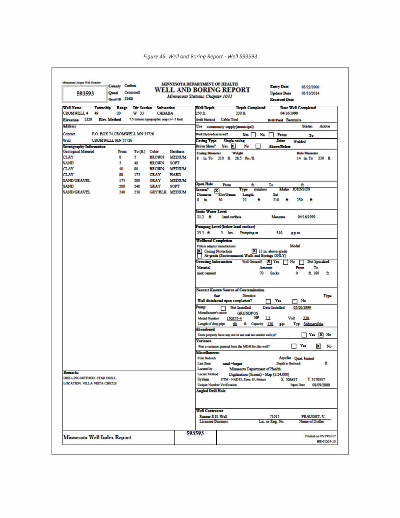
Figure 45. Well and Boring Report - Well 593593
T E S T 2 6 1 2 , C R O M W E L L 4 ( 5 9 3 5 9 3 ) M A Y 2 4 , 2 0 1 7
67
Figure 46. Well and Boring Report - Well 519761

T E S T 2 6 1 2 , C R O M W E L L 4 ( 5 9 3 5 9 3 ) M A Y 2 4 , 2 0 1 7
68
Figure 47. Well and Boring Report - Well 773071

T E S T 2 6 1 2 , C R O M W E L L 4 ( 5 9 3 5 9 3 ) M A Y 2 4 , 2 0 1 7
69
Figure 48. Well and Boring Report - Well 773070

T E S T 2 6 1 2 , C R O M W E L L 4 ( 5 9 3 5 9 3 ) M A Y 2 4 , 2 0 1 7
70
Figure 49. Well and Boring Report - Well 773069

T E S T 2 6 1 2 , C R O M W E L L 4 ( 5 9 3 5 9 3 ) M A Y 2 4 , 2 0 1 7
71
Figure 50. Well and Boring Report - Well 773068

T E S T 2 6 1 2 , C R O M W E L L 4 ( 5 9 3 5 9 3 ) M A Y 2 4 , 2 0 1 7
72
Figure 51. Well and Boring Report - Well 773067

T E S T 2 6 1 2 , C R O M W E L L 4 ( 5 9 3 5 9 3 ) M A Y 2 4 , 2 0 1 7
73
Figure 52. Well and Boring Report - Well 773066

T E S T 2 6 1 2 , C R O M W E L L 4 ( 5 9 3 5 9 3 ) M A Y 2 4 , 2 0 1 7
74
Figure 53. Well and Boring Report - Well 773065
T E S T 2 6 1 2 , C R O M W E L L 4 ( 5 9 3 5 9 3 ) M A Y 2 4 , 2 0 1 7
75
Figure 54. Well and Boring Report - Well 773064


