April ‡ƒ - HIE R Course · Solutions to Exercises ... Multivariate statistics 1.5Exercises...
60
Multivariate statistics Solutions to Exercises April ,
Transcript of April ‡ƒ - HIE R Course · Solutions to Exercises ... Multivariate statistics 1.5Exercises...

Multivariate statisticsSolutions to Exercises
April 26, 2019
Contents
1 Multivariate statistics 21.5 Exercises . . . . . . . . . . . . . . . . . . . . . . . . . . . . . . . . . . . . . . . . . . . . . . . . . . . . 21.5.1 Ordination . . . . . . . . . . . . . . . . . . . . . . . . . . . . . . . . . . . . . . . . . . . . . . . 21.5.2 Analysis of Structure 1: two-table analysis . . . . . . . . . . . . . . . . . . . . . . . . . . . 171.5.3 Analysis of Structure 2: variation partitioning . . . . . . . . . . . . . . . . . . . . . . . . . 261.5.4 Analysis of Structure 3: ’experimental’ systems . . . . . . . . . . . . . . . . . . . . . . . 44
1
Chapter 1
Multivariate statistics
1.5 Exercises
In these exercises, we use the following colour codes:∎ Easy: make sure you complete some of these before moving on. These exercises will followexamples in the text very closely.⧫ Intermediate: a bit harder. You will often have to combine functions to solve the exercise intwo steps.▲ Hard: difficult exercises! These exercises will require multiple steps, and significant departurefrom examples in the text.
We suggest you complete these exercises in an R markdown file. This will allow you to combine codechunks, graphical output, and written answers in a single, easy-to-read file.
1.5.1 Ordination
1.5.1.1 Allometry data
File: ‘Allometry.csv’This dataset contains measurements of tree dimensions and biomass. Data kindly provided by JohnMarshall, University of Idaho.Variables:
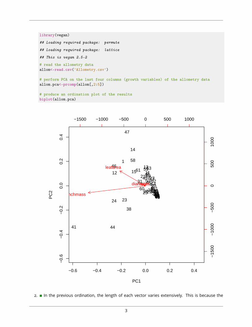
• species - The tree species (PSME = Douglas fir, PIMO = Western white pine, PIPO = Ponderosapine).• diameter - Tree diameter at 1.3m above ground (cm).• height - Tree height (m).• leafarea - Total leaf area (m2).• branchmass - Total (oven-dry) mass of branches (kg).1. ∎ Perform a PCA of the data in the allometry dataset (‘Allometry.csv’) without changing the scaleargument and plot the ordination result. Note that the first column contains species identities soyou need to exclude this column from the analysis. See Section ?? for help, if necessary.
2
library(vegan)
## Loading required package: permute
## Loading required package: lattice
## This is vegan 2.5-2
# read the allometry dataallom<-read.csv('Allometry.csv')
# perform PCA on the last four columns (growth variables) of the allometry dataallom.pca<-prcomp(allom[,2:5])
# produce an ordination plot of the resultsbiplot(allom.pca)
−0.6 −0.4 −0.2 0.0 0.2 0.4
−0.
6−
0.4
−0.
20.
00.
20.
4
PC1
PC
2
1
2
3
456
7
89
10
111213
14
15
16171819
20
21
22
2324
2526
27
282930
31
3233343536
37
38
3940
41
4243
44
45
46
47
48
49
50
5152
53
54
55
56
57
58
59
60
61
62
63
−1500 −1000 −500 0 500 1000
−15
00−
1000
−50
00
500
1000
diameterheight
leafarea
branchmass
2. ∎ In the previous ordination, the length of each vector varies extensively. This is because the
3
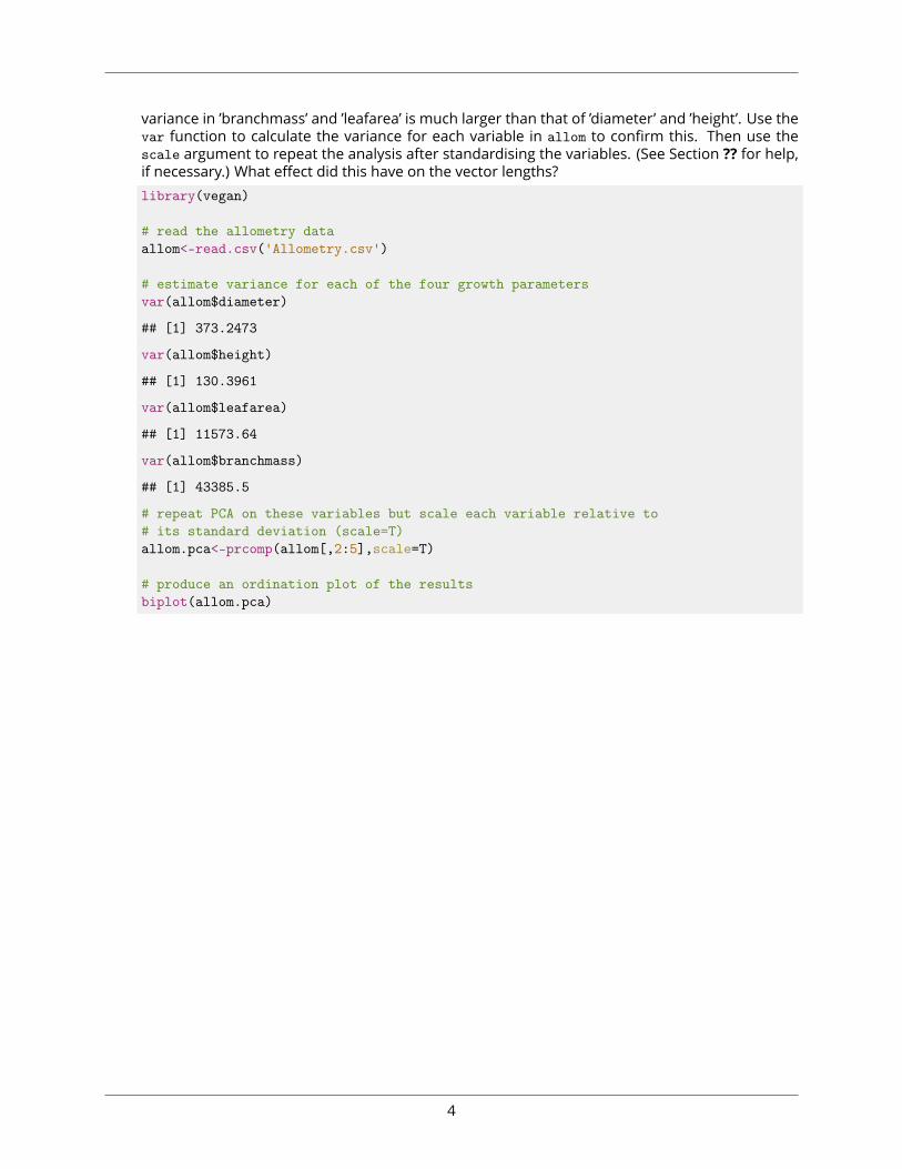
variance in ’branchmass’ and ’leafarea’ is much larger than that of ’diameter’ and ’height’. Use thevar function to calculate the variance for each variable in allom to confirm this. Then use thescale argument to repeat the analysis after standardising the variables. (See Section ?? for help,if necessary.) What effect did this have on the vector lengths?library(vegan)
# read the allometry dataallom<-read.csv('Allometry.csv')
# estimate variance for each of the four growth parametersvar(allom$diameter)
## [1] 373.2473
var(allom$height)
## [1] 130.3961
var(allom$leafarea)
## [1] 11573.64
var(allom$branchmass)
## [1] 43385.5
# repeat PCA on these variables but scale each variable relative to# its standard deviation (scale=T)allom.pca<-prcomp(allom[,2:5],scale=T)
# produce an ordination plot of the resultsbiplot(allom.pca)
4
−0.5 −0.4 −0.3 −0.2 −0.1 0.0 0.1 0.2
−0.
5−
0.4
−0.
3−
0.2
−0.
10.
00.
10.
2
PC1
PC
2
1
2 34
56
789 10
11
12
13
14 15
1617181920
21
2223
24
25
26
27
28
293031
323334
3536
37
38
3940
41
424344
45
46
47
48
49
50
51
52
53
5455
56
5758
59
60
61
62
63
−15 −10 −5 0 5
−15
−10
−5
05
diameter
height
leafarea
branchmass
# vector lengths are much more similar than for the default analysis (scale = F)
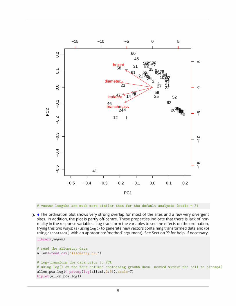
3. ⧫ The ordination plot shows very strong overlap for most of the sites and a few very divergentsites. In addition, the plot is partly off-centre. These properties indicate that there is lack of nor-mality in the response variables. Log-transform the variables to see the effects on the ordination,trying this two ways: (a) using log() to generate new vectors containing transformed data and (b)using decostand() with an appropriate ’method’ argument). See Section ?? for help, if necessary.library(vegan)
# read the allometry dataallom<-read.csv('Allometry.csv')
# log-transform the data prior to PCA# using log() on the four columns containing growth data, nested within the call to prcomp()allom.pca.log1<-prcomp(log(allom[,2:5]),scale=T)biplot(allom.pca.log1)
5
−0.2 −0.1 0.0 0.1 0.2 0.3 0.4
−0.
2−
0.1
0.0
0.1
0.2
0.3
0.4
PC1
PC
2
1
2
3
4
567
89
10
11
12
13
141516
1718
19
20
21
22
23
24 25
2627
28
29
30
31
32
3334
3536
37
38
39
40
41
4243
44
45
4647
48
49
50 515253
54
55
56
57
58
59
60
61
62
63
−5 0 5 10
−5
05
10
diameter
height
leafareabranchmass
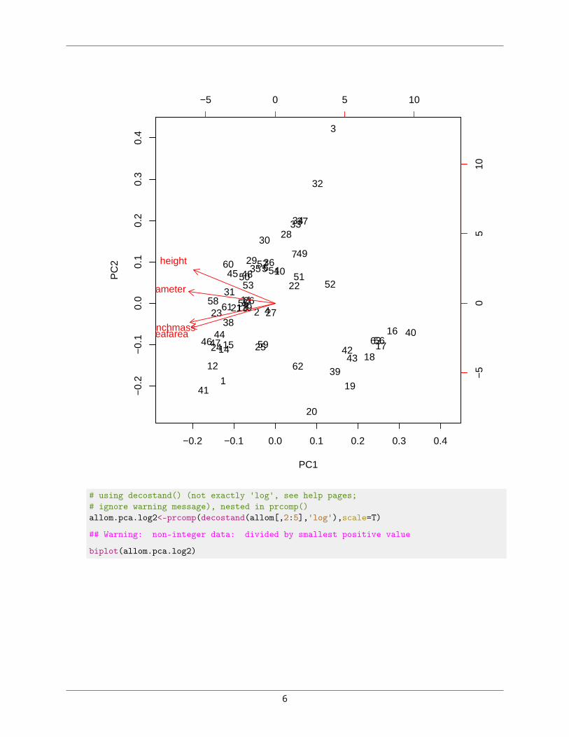
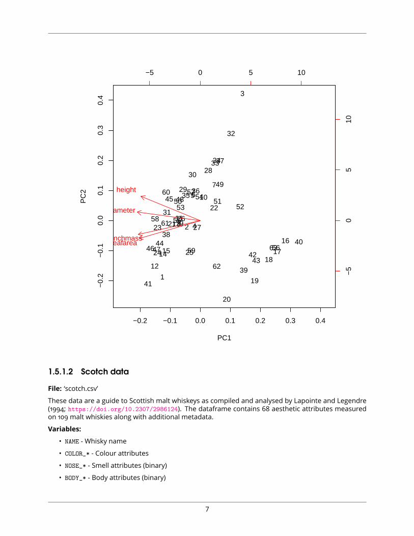
# using decostand() (not exactly 'log', see help pages;# ignore warning message), nested in prcomp()allom.pca.log2<-prcomp(decostand(allom[,2:5],'log'),scale=T)
## Warning: non-integer data: divided by smallest positive value
biplot(allom.pca.log2)
6
−0.2 −0.1 0.0 0.1 0.2 0.3 0.4
−0.
2−
0.1
0.0
0.1
0.2
0.3
0.4
PC1
PC
2
1
2
3
4
567
89
10
11
12
13
141516
1718
19
20
21
22
23
24 25
2627
28
29
30
31
32
3334
3536
37
38
39
40
41
4243
44
45
4647
48
49
50 515253
54
55
56
57
58
59
60
61
62
63
−5 0 5 10
−5
05
10
diameter
height
leafareabranchmass
1.5.1.2 Scotch data
File: ‘scotch.csv’These data are a guide to Scottish malt whiskeys as compiled and analysed by Lapointe and Legendre(1994; https://doi.org/10.2307/2986124). The dataframe contains 68 aesthetic attributes measuredon 109malt whiskies along with additional metadata.Variables:
• NAME - Whisky name• COLOR_* - Colour attributes• NOSE_* - Smell attributes (binary)• BODY_* - Body attributes (binary)
7
• PAL_* - Palatte attributes (binary)• FIN_* - Finish attributes (binary)• AGE - Whisky age, with NA values scored as -9.• REGION - Distillery region of origin.• DISTRICT - Distillery district of origin.1. ∎ Read in the scotch dataset (‘scotch.csv’). The dataframe includes variables that represent as-sessments of taste, smell and appearance (binary response data) and other attributes (metadata)of malt whiskeys. Generate a new dataframe that includes only the binary response data. Hint:names of data variables include the _ symbol to separate variable category from the variablename while metadata variables do not include this symbol, use grep(’_’, names(df)) to indexthe dataframe.
# read datascotch <- read.csv('scotch.csv')
# response variables contain underscore symbol# use 'grep' to identify response variables and retain in new input matrixscotchvars <- scotch[, grep('_', names(scotch))]
# check to make sure that the table has the expected dimensions (109, 68)dim(scotchvars)
## [1] 109 68
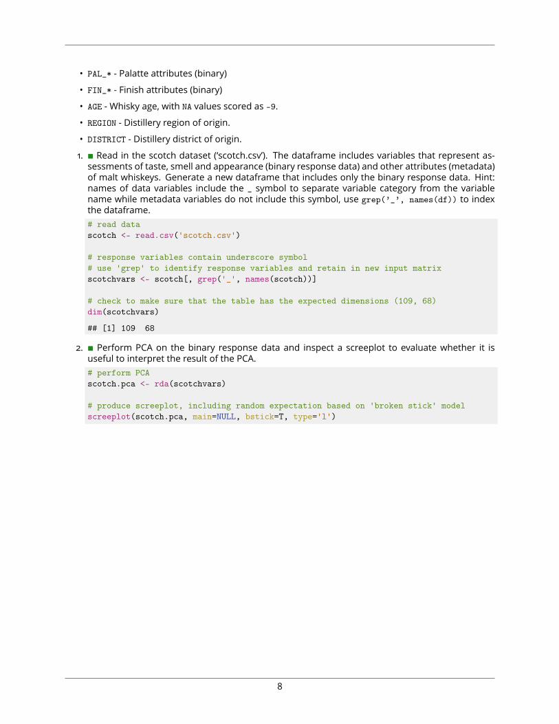
2. ∎ Perform PCA on the binary response data and inspect a screeplot to evaluate whether it isuseful to interpret the result of the PCA.# perform PCAscotch.pca <- rda(scotchvars)
# produce screeplot, including random expectation based on 'broken stick' modelscreeplot(scotch.pca, main=NULL, bstick=T, type='l')
8
Component
Iner
tia
0.25
0.30
0.35
0.40
0.45
0.50
0.55
0.60
PC1 PC2 PC3 PC4 PC5 PC6 PC7 PC8 PC9 PC10
OrdinationBroken Stick
# the first two axes explain less variation than the null expectation
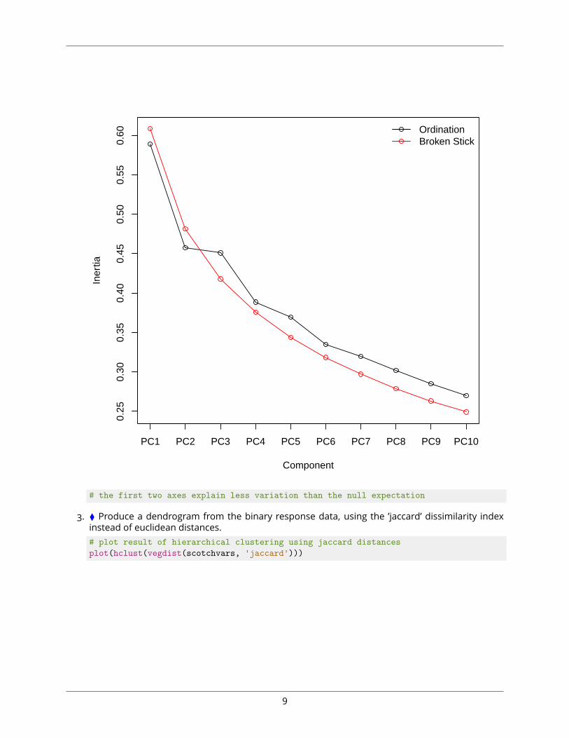
3. ⧫ Produce a dendrogram from the binary response data, using the ’jaccard’ dissimilarity indexinstead of euclidean distances.# plot result of hierarchical clustering using jaccard distancesplot(hclust(vegdist(scotchvars, 'jaccard')))
9
38 4631 65 76
57 105
1933
36 4750 56
37 102 5
1 8064 77
45 7325 97
5 116
71 7275
14 32 278
107
93 103
484
49 5915
20 109
9524 92
78 9962
70 9852
30 88 29 4218 26
8723 82
6312
41 5322 48
10 4469 10
428 10
667
34 553 17 89 94
85 862 96
83 100
9 1368 90
9143 54
166 79
4010
860 61
35 3921 10
116 58
747 81
0.4
0.5
0.6
0.7
0.8
0.9
1.0
Cluster Dendrogram
hclust (*, "complete")vegdist(scotchvars, "jaccard")
Hei
ght
# If the plotting window is too small, open one like this: windows()# (Or click 'Zoom')
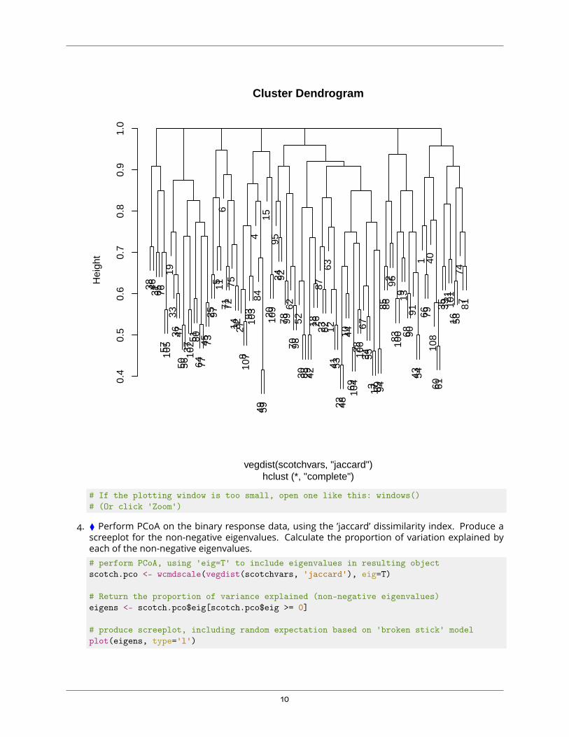
4. ⧫ Perform PCoA on the binary response data, using the ’jaccard’ dissimilarity index. Produce ascreeplot for the non-negative eigenvalues. Calculate the proportion of variation explained byeach of the non-negative eigenvalues.# perform PCoA, using 'eig=T' to include eigenvalues in resulting objectscotch.pco <- wcmdscale(vegdist(scotchvars, 'jaccard'), eig=T)
# Return the proportion of variance explained (non-negative eigenvalues)eigens <- scotch.pco$eig[scotch.pco$eig >= 0]
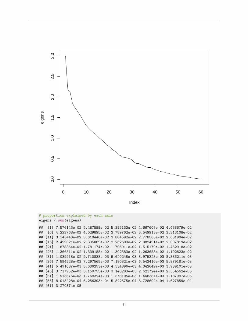
# produce screeplot, including random expectation based on 'broken stick' modelplot(eigens, type='l')
10
0 10 20 30 40 50 60
0.0
0.5
1.0
1.5
2.0
2.5
3.0
Index
eige
ns
# proportion explained by each axiseigens / sum(eigens)
## [1] 7.576143e-02 5.487599e-02 5.395133e-02 4.667608e-02 4.438679e-02## [6] 4.222768e-02 4.029895e-02 3.789762e-02 3.549913e-02 3.313108e-02## [11] 3.143440e-02 3.010446e-02 2.884592e-02 2.778563e-02 2.631904e-02## [16] 2.499021e-02 2.395089e-02 2.262603e-02 2.082491e-02 2.007819e-02## [21] 1.878364e-02 1.781174e-02 1.706011e-02 1.515179e-02 1.452918e-02## [26] 1.366511e-02 1.339188e-02 1.302583e-02 1.263653e-02 1.192823e-02## [31] 1.039918e-02 9.710838e-03 9.620248e-03 8.975323e-03 8.336211e-03## [36] 7.594528e-03 7.297565e-03 7.180321e-03 6.542416e-03 5.879181e-03## [41] 5.491037e-03 5.036253e-03 4.534896e-03 4.342642e-03 3.939101e-03## [46] 3.717952e-03 3.158755e-03 3.143203e-03 2.621724e-03 2.354562e-03## [51] 1.913676e-03 1.768324e-03 1.578105e-03 1.448387e-03 1.187987e-03## [56] 8.015428e-04 6.256393e-04 5.822675e-04 3.728604e-04 1.627859e-04## [61] 3.270874e-05
11
1.5.1.3 Endophyte data
File: ‘endophytes_env.csv’ and ‘endophytes.csv’Community fingerprints from fungi colonising living leaves and litter from nine Eucalyptus spp. in theHFE common garden and surrounding area. ‘endophytes.csv’ contains a ’species-sample’ matrix, with98 samples in rows and 874 operational taxonomic units (OTUs) in columns.The variables below refer to the data in ‘endophytes_env.csv’. The rows are matched across the twotables.Variables:
• species - Tree species• type - Whether leaves came from canopy (fresh) or ground (litter)• percentC - Leaf carbon content, per gram dry mass• percentN - Leaf nitrogen content, per gram dry mass• CNratio - Ratio of C to N in leaves1. ∎ Read in the data from ‘endophytes.csv’; see Section ?? (p. ??) for a description of the data. Usethe decorana function to calculate gradient lengths and determine whether PCA is appropriatefor these data (see Section ?? for help, if necessary).
# read in endophyte community dataendo<-read.csv('endophytes.csv')
# estimate gradient lengthdecorana(endo)
#### Call:## decorana(veg = endo)#### Detrended correspondence analysis with 26 segments.## Rescaling of axes with 4 iterations.#### DCA1 DCA2 DCA3 DCA4## Eigenvalues 0.5160 0.3277 0.2663 0.2971## Decorana values 0.5406 0.4279 0.2738 0.2552## Axis lengths 3.6757 4.0614 2.7659 2.9553
# the gradient (axis) lengths are around or greater than 3,# suggesting that PCA is not appropriate
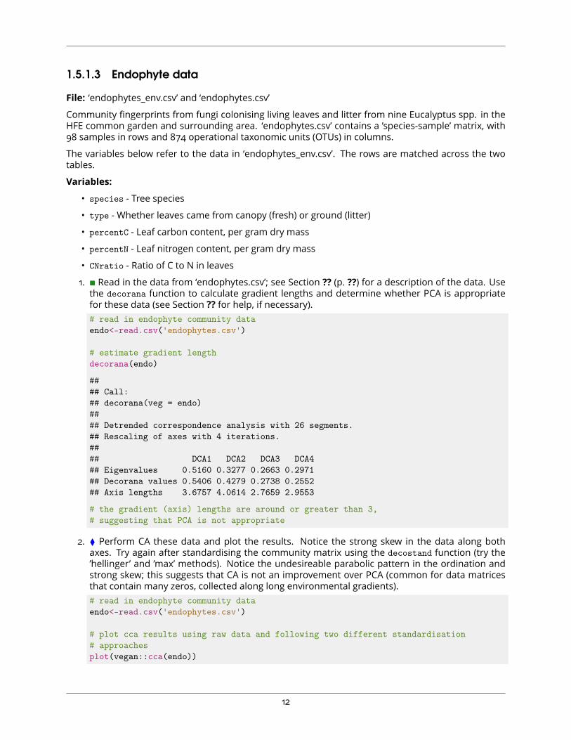
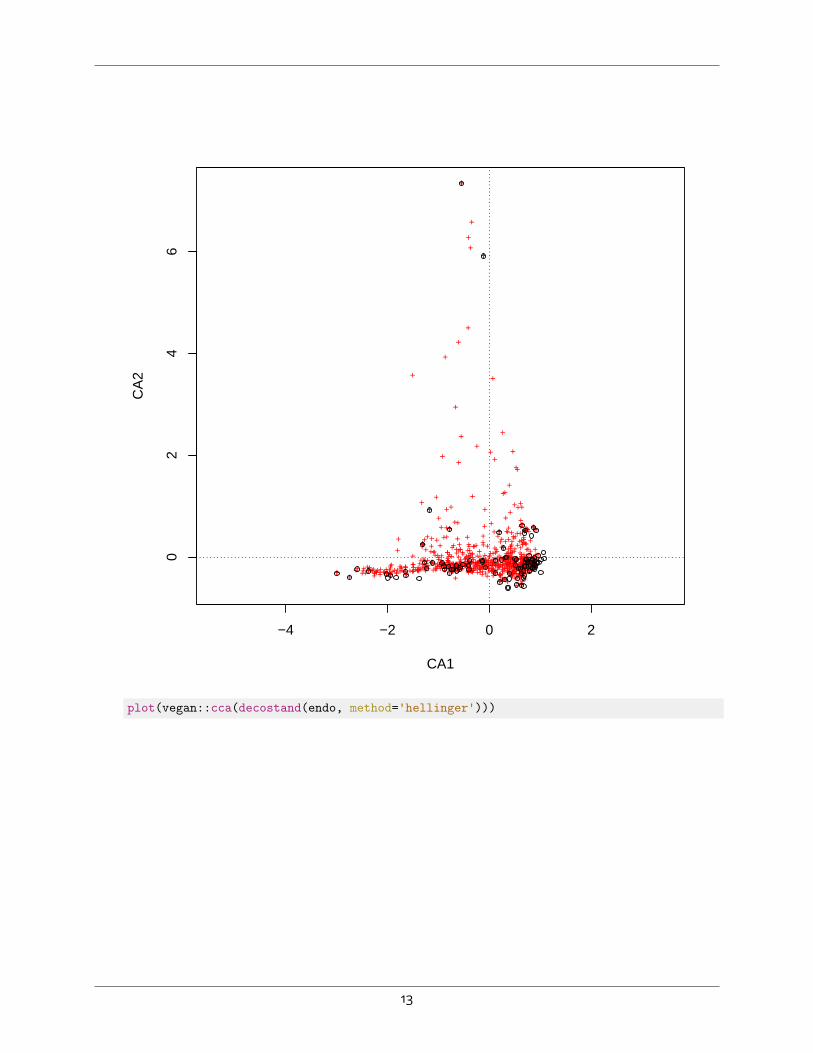
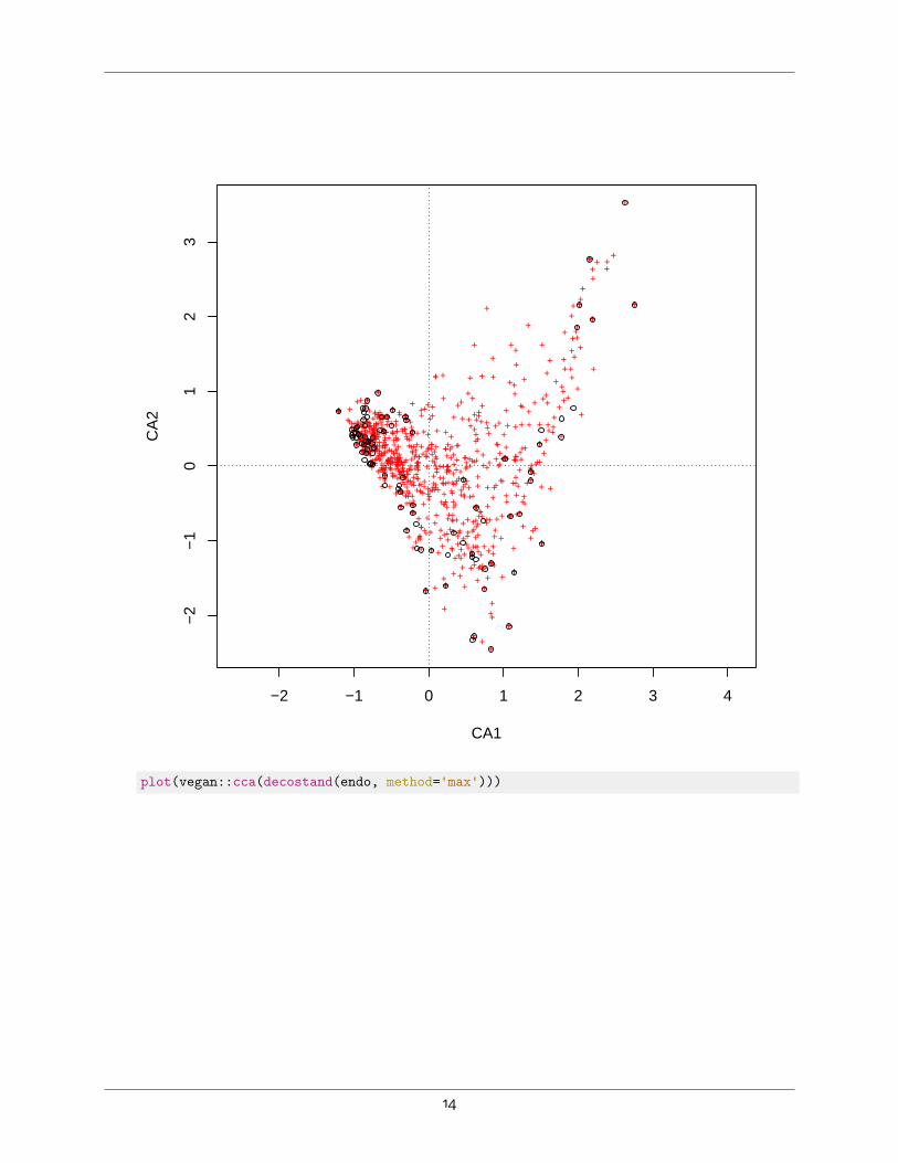
2. ⧫ Perform CA these data and plot the results. Notice the strong skew in the data along bothaxes. Try again after standardising the community matrix using the decostand function (try the’hellinger’ and ’max’ methods). Notice the undesireable parabolic pattern in the ordination andstrong skew; this suggests that CA is not an improvement over PCA (common for data matricesthat contain many zeros, collected along long environmental gradients).# read in endophyte community dataendo<-read.csv('endophytes.csv')
# plot cca results using raw data and following two different standardisation# approachesplot(vegan::cca(endo))
12
−4 −2 0 2
02
46
CA1
CA
2
+++ ++ ++
++
+++++
+
++
++
++
+
++
+
+
++++
++++
++
+
+++
+
++
+
+
++ +
+++
+
+
++
++ +
+++ ++
++++
+
++
++ +++
+++ +
++++
+
++
+
++
+
+
+ +++
+ ++
+ ++
+
+ ++ + ++
+
+
+
+
+
++
++
+++
++
+++
++++ +
++
+
+ +
++ +
+
+
+++ ++ ++ +
++
++
+
++++
++ +
+
+
++++++
++ ++ ++
+
+
+
++
++ +++
+
++
+++
+ ++++
+ ++
+
+
+++ ++
+
+++
+
+
+
+ +
+
++ +
+
+++ +
+
+ +++
+++
++ ++
+ ++ + + + +
+++++
++
+
+
+++
+++
+++ +
+
++ +++
++
+ ++
+
+
+
+ +
+
+
+
+
++
++
+
+ + ++
+
+ +++
++
+ +
++
+
+
+
++
++
+
+
+
+
+
+
+
+
+
+
+
+
+
+
+
+
+
+++++
+++
++++
+++
++
+
++
+ + +++
+
++
+
+++ +++
++ ++ +++
+
++
+
+++
+++++ ++ +
++ +++
++
++
+ +
+
+
+
+
++
+
+
+++
+ ++
+
+++
+ +
+
+
+++
+
+
++
+
+ +++++ ++
+
+++
+
++++ + +
+
++++
++ +
+
+
+
+
++
++++++ ++ ++
++++ ++
+++
++
++++ ++
+++ ++
++
++
++
++
+
+
+++
+++++ +
+
+++ +
++++ +++++
+
++++
+++
+
+
+++ +++
+
+
+
+
+++ +++
++
+
+
+
+
+++++
++
+
+
+
+
+++ + ++
+
+ +
+
++
++ +++ +
+++
++
+
+
+
++
+++
+++ ++
++
+ +++ ++
+ +
++
+
+
+
+
+++
+ +++
+
+
++
++ +++ ++
+
++
+ +++++ +
+ +++
++
++++
+
++
+ +++
+
+++
++
++++++
++ ++
+ ++ +++ ++ ++
+
+
++
+++++++ + +
++ + +
+++
+
+
+ ++
+
+
+++ ++ +
+
++++ +
+
+++ ++ + + +++
+
+
+
+
++ +++
+++++++
++
++++ +
+
+++ + +
+
++ +
+++
+ ++
++ ++
+++
++++++
+
+
+
+++
+ ++ +
+
++
+++
++ +
+
+
+
++ ++
+
+
+
+
++
+
++
+ ++++++ +
+
+ +++
++
+
++ ++
+ + +++
+ ++ +
+
+
+++
+
+
+++
+
++++++
+++
+
plot(vegan::cca(decostand(endo, method='hellinger')))
13
−2 −1 0 1 2 3 4
−2
−1
01
23
CA1
CA
2
++
+
+
++
+
+
+
+
+
+
+
+
++
+
+
+
+
+
++
+
+
+
+
++
+
+
++
++
++
+
+
++
+
+
+
+
+ +
+
+++
++
+
+
++
+
++
+
+
+
+
+
+
++
+
+
++
+++ +
+
++
+
+
+
+
+
++ +
+
++
+
+
+
++
+
+
+
+
++
+
+
++
+
++
++
+ ++
+
+
+
+
+ +
+
+
++
+
+
+
++
+
+
+
+
+
+
+
+
+
+
+
+
+
+
+
+
+
+
+
+ +
++
+
+
+
+
+
+
+
+
+
+ +
+
+
+
+
+
++
+
+
++
+
+
+
+
+
+
+
+
++
++
++
+
+
+
+
+
+
+
+
+
+
++
++
+
++
+
+
++ +
+
+
+
+
+
+
+
+
+
+
++
+
++ +
+
+
+
+
+
+
++
+
+
+
+
+
+
+
++
+
+
+
+
+
+
+
++
++
+
+
+
+
+
++
+
+
+ +
+
++
++
+
+
+
+
+
+
+
++
+++
+
+
++
+
+
+
+
++
+
+
+ +
+
++++
++
+
+
+
+
+++
++
++
+
+
+
+
+
+
+
+
+
+
+
+
+
++
+
+
+
+
+
++
+
+
++
+
++++
+
++++
+
+
+
+
+
+
+++
+
+
+
+
+
++
+
+
+
+
+
++
+
+
++ +
+
+
+
++
+ +
+
+
+
++
++
+
+
+
+
+
+
+
+
+
+
+
+
+
+
+
+
+
+
+
+
+
+
+
+
+
+
+
+
+
+
+
+
+
+++
+
+
+
+
+
+
+
+
+
+
++
+
+
+
+
++ +
+
+
+
+++
+
++
++
+
++
++
+
+
++
+
+
+
+
++++
+
+
+
++
+
+
+
+
+
+
+
+ +++
+
+
+
+
+
+
+
+
+
+
+
++
+
+
+
+
+
+
+
+
+
+ ++
++
+++
+
+
+
++
+
++
++
++
+
+
+
+
+
+
+++
+
+
+
+
+
+
+
+
+
+
+
+
+
++++
+
+
+
++
+
+
++
+
+
+ +++ +
+
+
+
++
+
+
+
+
+
+
+
+
+
+ +
+
++
++
+
++
+
++
+
+
++ +
+
+
+
+
++
+
+++
+
++
+
+++
+
+
+
+
+
+
++
+
+
+
+ +
+
+
+
++
+
+
+
+
+
+
+
++
+
+
+
+
+
+
+
+
+
+
+
+
+
+
+
+ ++
+++++ +
++
+
+
+
+
+
+
+
+++
+
+++
+
+
+
+
++
+
++
+
+
+
++
+
+
+
+
+
+
+
+++
+
+
++
+
++
+
+
+
++
+
+
+
+
+
+
+
++
+
+
+
+
+
+
+
+
+
+
+
+ +++
+
++
++
+
+
+
+
+
++
+
++
+
+
+
+
++++
+
++
+
+
+
++
+
+
++
++
+
+
+
+
+
+
+
+ +
+
++ +
+
+
+
+
++
+
+
+
+
+
+
+
+ ++
++++
++
+
+
+
++++
+
+
+
+
+
+
+
+
+
+
+
++
+
+
+++
+
+
+
+
+
+
++
+
++
+
+
+
+
+
++
+
+++
++
++
+
plot(vegan::cca(decostand(endo, method='max')))
14
−4 −2 0 2 4
−6
−4
−2
0
CA1
CA
2
+
+
+
+
+
+
+
+
+
+
+ +
+
++ +
++
+
+
+
++
++
+
+
+
+
+
+
+ +++
++
++
+
+
+
+
++
+ ++
++++ +
+
+++
+
+
+
+
+
+
++
++
+
+
+++
+++
+
+
+
+
+
++
+
+
+
+
+ +
+
++
+
+
++
++
+
+
+
+
+
+
+
++
++
+++ ++
+
+
++
+
+
+
+ ++
+
+
++
+
+
+ +
+
+
++
+
+
+
++
++ ++ ++ ++
+
++ +
+
++
++
+
++
++
+
++
+
++
+
++
+
+
+
+++
+
++
+
+
+
+
+
+ +
+
+
+++
++
++
+
++ ++
+++
+
+++
++
+
+
+
+
++
+
+
+
++
+
+
+
+
+
+
+
+
+
+
+
+
+
+
+
+
++
++
+
+
++
+
+
+
+ ++
+
+
+
++
+
+
++
++
+++
+ +
+
+
+
+
+
+
+
+
++
++
++ ++
++
+
+
++ +
+
+
+
+++
+
+
+
+
+
++
++
+
+++
+
+ +
+
+
+
++ +
+
+++
++
+
++ +
+
+
++ +++
++
+
+++
++
+ ++
+++
++
+++
++++
+
+
+++
+
+ ++
+++
+
+
+
+++
+++
+
+
+ +
+
+
++++
+
+
++
++ +
+
+ +
+ +
++
+
+
+
+
+
+
+
+
+
+
++
+
+ ++
+
+
+
+
+
+
+
+
+
+
+
+
+
++
+
++
++
+
+
+
+
++
+ +++
+
+
+
+
+
+
+
++
+++
+
+
+
+
+
+
+
++
++++
+
+
+
+
+
++
++
+
++
++
++
++
+
+
+
++ +
+++
+
+
+
+
+
+
+
+
+
+
++
+
+
++
++
+ ++
+
+++
++
++
+
+
+
+
+
+
+
+
+++
+
+
+
+
+
+
+
+ ++
+
+
+
+
+
+
+
+
+
+
+
++
++
+
+
++
++
++
+
+
+ +++
+
++
++ ++
+
++
+
+++
++
++
++
+
+
+
+
+
++
+
++ ++ + +++
+++
+
+ ++
++++
+
+
+
+
+
+
+
+
++
+
+ ++
+++
+
+ +
++
++
+++
+
++
+
+ +
+
+
+
+
+
+
+
++
+
+
+
+
+
++
+
++ ++
++
+
+
+
+
+
+
++
++
+
++
+++
+
+
+
+
++
+
+
+
+
+
+
+++
+
+
+++
++
+
++
+
+
+
+
+
++
++
+
++
+
+
+
+ ++
+
+
+
+
+ +++
+
+++
+ ++ +++
++
+
++
+
++
+++
+
+
+
++ ++
+++
++
+
+
+ ++
++
++
+
+
+
+
+ +
+ ++++ +
++
+
+
+
+
+
+
++ + +
+
+
++
+
+
+
+
+
++
+++
++ + ++
+
+
+
+
+
+ ++ +
+
+
++
++
+
+
+
++
+
+
+
++
+
+
+
++
+
+
+
+
++
+++
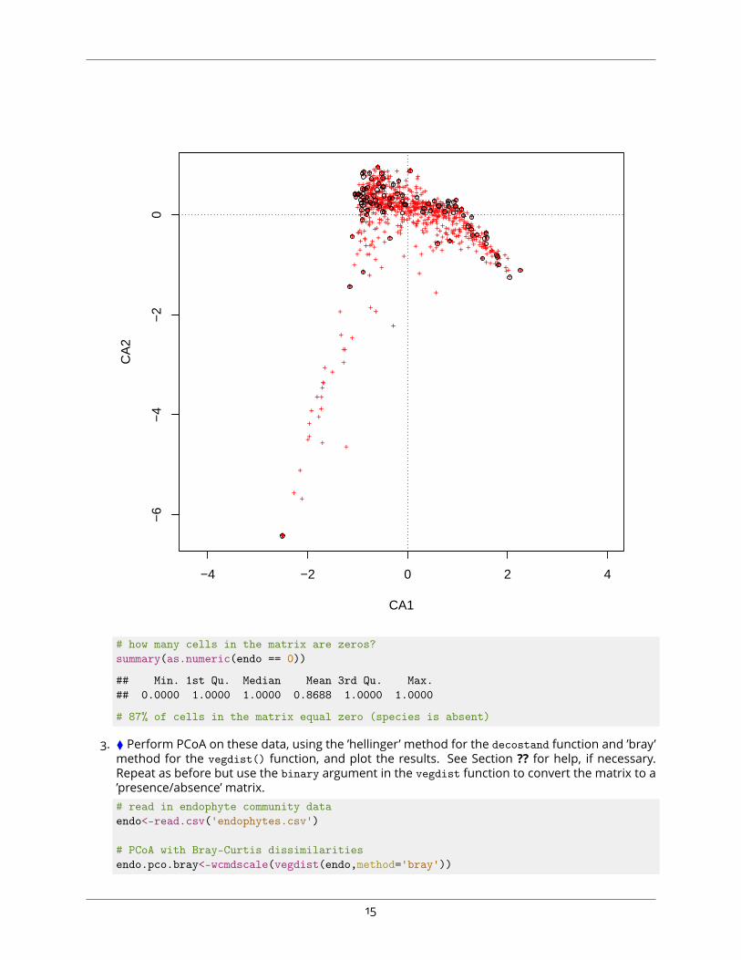
# how many cells in the matrix are zeros?summary(as.numeric(endo == 0))
## Min. 1st Qu. Median Mean 3rd Qu. Max.## 0.0000 1.0000 1.0000 0.8688 1.0000 1.0000
# 87% of cells in the matrix equal zero (species is absent)
3. ⧫ Perform PCoA on these data, using the ’hellinger’method for the decostand function and ’bray’method for the vegdist() function, and plot the results. See Section ?? for help, if necessary.Repeat as before but use the binary argument in the vegdist function to convert the matrix to a’presence/absence’matrix.# read in endophyte community dataendo<-read.csv('endophytes.csv')
# PCoA with Bray-Curtis dissimilaritiesendo.pco.bray<-wcmdscale(vegdist(endo,method='bray'))
15
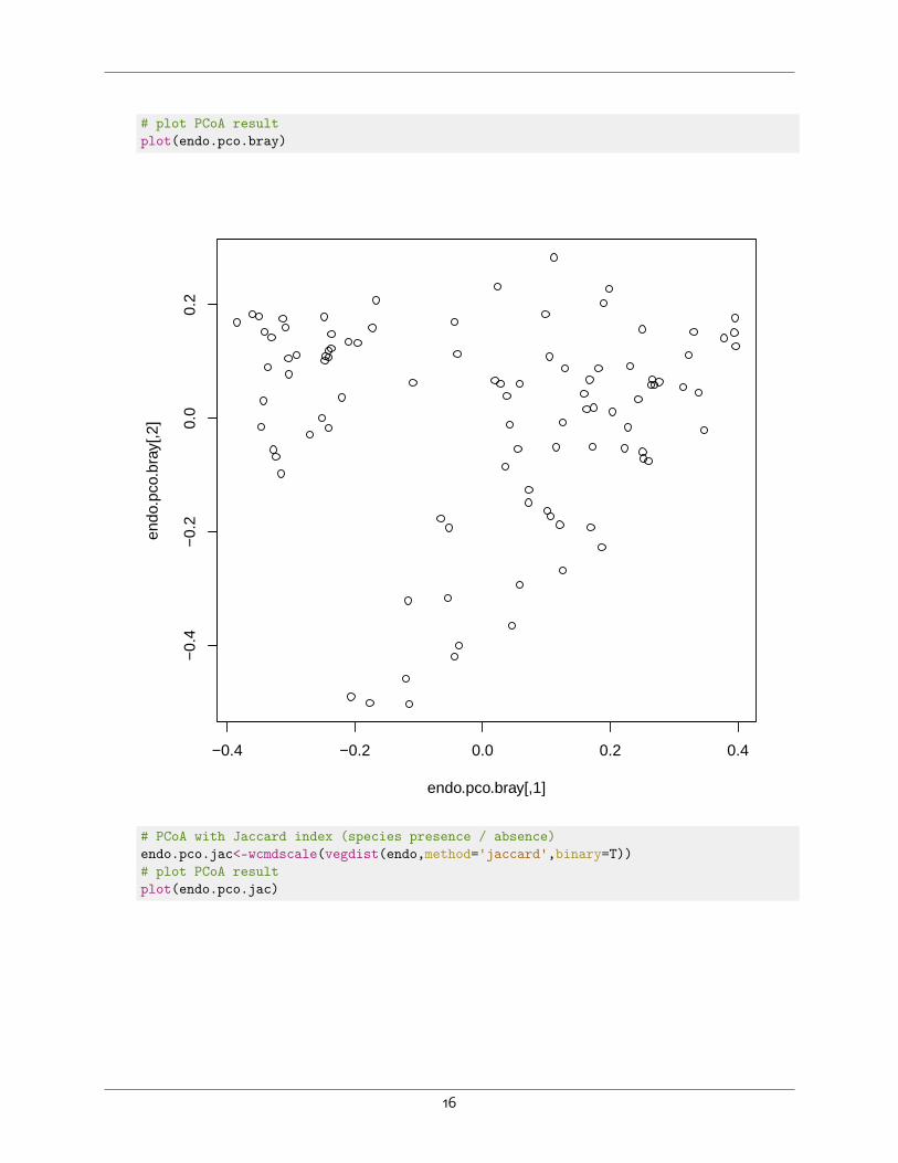
# plot PCoA resultplot(endo.pco.bray)
−0.4 −0.2 0.0 0.2 0.4
−0.
4−
0.2
0.0
0.2
endo.pco.bray[,1]
endo
.pco
.bra
y[,2
]
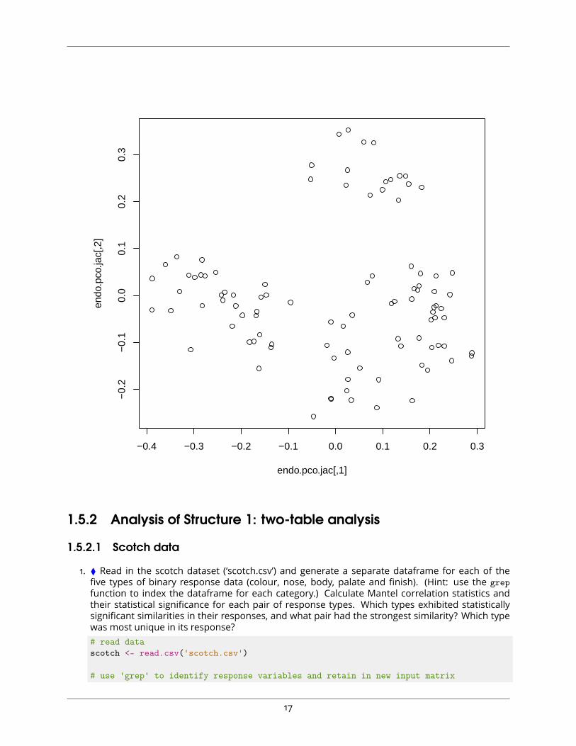
# PCoA with Jaccard index (species presence / absence)endo.pco.jac<-wcmdscale(vegdist(endo,method='jaccard',binary=T))# plot PCoA resultplot(endo.pco.jac)
16
−0.4 −0.3 −0.2 −0.1 0.0 0.1 0.2 0.3
−0.
2−
0.1
0.0
0.1
0.2
0.3
endo.pco.jac[,1]
endo
.pco
.jac[
,2]
1.5.2 Analysis of Structure 1: two-table analysis
1.5.2.1 Scotch data
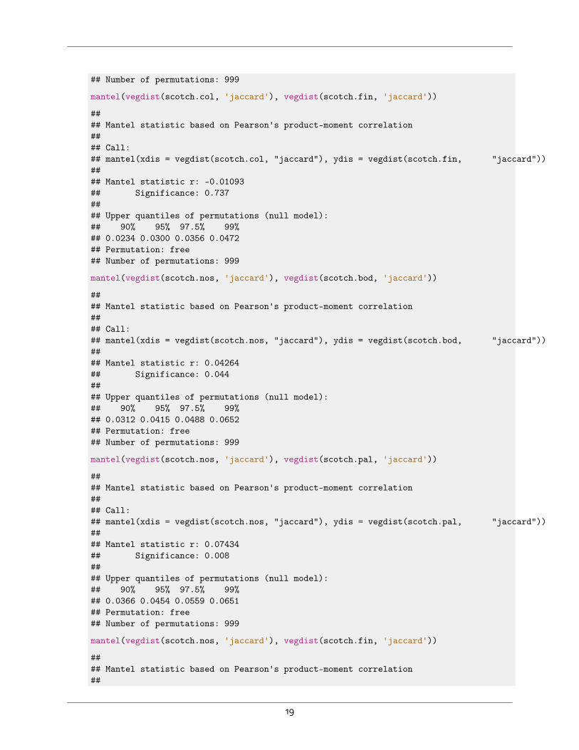
1. ⧫ Read in the scotch dataset (‘scotch.csv’) and generate a separate dataframe for each of thefive types of binary response data (colour, nose, body, palate and finish). (Hint: use the grepfunction to index the dataframe for each category.) Calculate Mantel correlation statistics andtheir statistical significance for each pair of response types. Which types exhibited statisticallysignificant similarities in their responses, and what pair had the strongest similarity? Which typewas most unique in its response?# read datascotch <- read.csv('scotch.csv')
# use 'grep' to identify response variables and retain in new input matrix
17
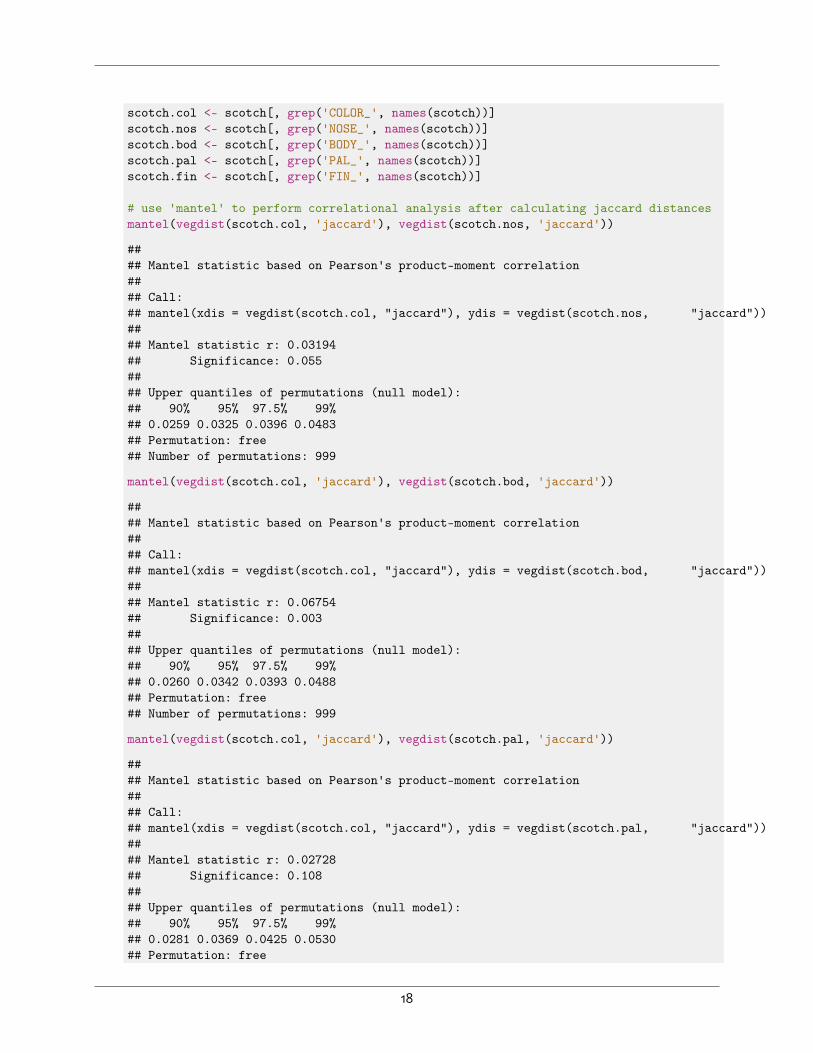
scotch.col <- scotch[, grep('COLOR_', names(scotch))]scotch.nos <- scotch[, grep('NOSE_', names(scotch))]scotch.bod <- scotch[, grep('BODY_', names(scotch))]scotch.pal <- scotch[, grep('PAL_', names(scotch))]scotch.fin <- scotch[, grep('FIN_', names(scotch))]
# use 'mantel' to perform correlational analysis after calculating jaccard distancesmantel(vegdist(scotch.col, 'jaccard'), vegdist(scotch.nos, 'jaccard'))
#### Mantel statistic based on Pearson's product-moment correlation#### Call:## mantel(xdis = vegdist(scotch.col, "jaccard"), ydis = vegdist(scotch.nos, "jaccard"))#### Mantel statistic r: 0.03194## Significance: 0.055#### Upper quantiles of permutations (null model):## 90% 95% 97.5% 99%## 0.0259 0.0325 0.0396 0.0483## Permutation: free## Number of permutations: 999
mantel(vegdist(scotch.col, 'jaccard'), vegdist(scotch.bod, 'jaccard'))
#### Mantel statistic based on Pearson's product-moment correlation#### Call:## mantel(xdis = vegdist(scotch.col, "jaccard"), ydis = vegdist(scotch.bod, "jaccard"))#### Mantel statistic r: 0.06754## Significance: 0.003#### Upper quantiles of permutations (null model):## 90% 95% 97.5% 99%## 0.0260 0.0342 0.0393 0.0488## Permutation: free## Number of permutations: 999
mantel(vegdist(scotch.col, 'jaccard'), vegdist(scotch.pal, 'jaccard'))
#### Mantel statistic based on Pearson's product-moment correlation#### Call:## mantel(xdis = vegdist(scotch.col, "jaccard"), ydis = vegdist(scotch.pal, "jaccard"))#### Mantel statistic r: 0.02728## Significance: 0.108#### Upper quantiles of permutations (null model):## 90% 95% 97.5% 99%## 0.0281 0.0369 0.0425 0.0530## Permutation: free
18
## Number of permutations: 999
mantel(vegdist(scotch.col, 'jaccard'), vegdist(scotch.fin, 'jaccard'))
#### Mantel statistic based on Pearson's product-moment correlation#### Call:## mantel(xdis = vegdist(scotch.col, "jaccard"), ydis = vegdist(scotch.fin, "jaccard"))#### Mantel statistic r: -0.01093## Significance: 0.737#### Upper quantiles of permutations (null model):## 90% 95% 97.5% 99%## 0.0234 0.0300 0.0356 0.0472## Permutation: free## Number of permutations: 999
mantel(vegdist(scotch.nos, 'jaccard'), vegdist(scotch.bod, 'jaccard'))
#### Mantel statistic based on Pearson's product-moment correlation#### Call:## mantel(xdis = vegdist(scotch.nos, "jaccard"), ydis = vegdist(scotch.bod, "jaccard"))#### Mantel statistic r: 0.04264## Significance: 0.044#### Upper quantiles of permutations (null model):## 90% 95% 97.5% 99%## 0.0312 0.0415 0.0488 0.0652## Permutation: free## Number of permutations: 999
mantel(vegdist(scotch.nos, 'jaccard'), vegdist(scotch.pal, 'jaccard'))
#### Mantel statistic based on Pearson's product-moment correlation#### Call:## mantel(xdis = vegdist(scotch.nos, "jaccard"), ydis = vegdist(scotch.pal, "jaccard"))#### Mantel statistic r: 0.07434## Significance: 0.008#### Upper quantiles of permutations (null model):## 90% 95% 97.5% 99%## 0.0366 0.0454 0.0559 0.0651## Permutation: free## Number of permutations: 999
mantel(vegdist(scotch.nos, 'jaccard'), vegdist(scotch.fin, 'jaccard'))
#### Mantel statistic based on Pearson's product-moment correlation##
19
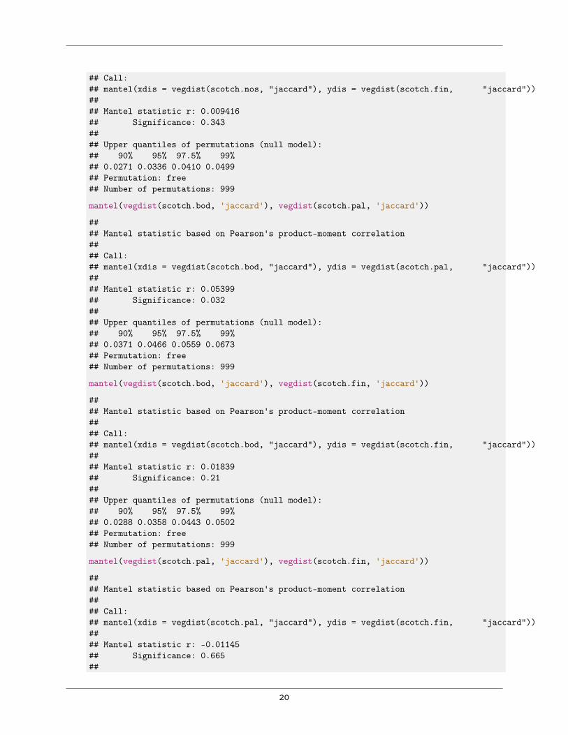
## Call:## mantel(xdis = vegdist(scotch.nos, "jaccard"), ydis = vegdist(scotch.fin, "jaccard"))#### Mantel statistic r: 0.009416## Significance: 0.343#### Upper quantiles of permutations (null model):## 90% 95% 97.5% 99%## 0.0271 0.0336 0.0410 0.0499## Permutation: free## Number of permutations: 999
mantel(vegdist(scotch.bod, 'jaccard'), vegdist(scotch.pal, 'jaccard'))
#### Mantel statistic based on Pearson's product-moment correlation#### Call:## mantel(xdis = vegdist(scotch.bod, "jaccard"), ydis = vegdist(scotch.pal, "jaccard"))#### Mantel statistic r: 0.05399## Significance: 0.032#### Upper quantiles of permutations (null model):## 90% 95% 97.5% 99%## 0.0371 0.0466 0.0559 0.0673## Permutation: free## Number of permutations: 999
mantel(vegdist(scotch.bod, 'jaccard'), vegdist(scotch.fin, 'jaccard'))
#### Mantel statistic based on Pearson's product-moment correlation#### Call:## mantel(xdis = vegdist(scotch.bod, "jaccard"), ydis = vegdist(scotch.fin, "jaccard"))#### Mantel statistic r: 0.01839## Significance: 0.21#### Upper quantiles of permutations (null model):## 90% 95% 97.5% 99%## 0.0288 0.0358 0.0443 0.0502## Permutation: free## Number of permutations: 999
mantel(vegdist(scotch.pal, 'jaccard'), vegdist(scotch.fin, 'jaccard'))
#### Mantel statistic based on Pearson's product-moment correlation#### Call:## mantel(xdis = vegdist(scotch.pal, "jaccard"), ydis = vegdist(scotch.fin, "jaccard"))#### Mantel statistic r: -0.01145## Significance: 0.665##
20
## Upper quantiles of permutations (null model):## 90% 95% 97.5% 99%## 0.0332 0.0419 0.0553 0.0653## Permutation: free## Number of permutations: 999
1.5.2.2 Endophyte data
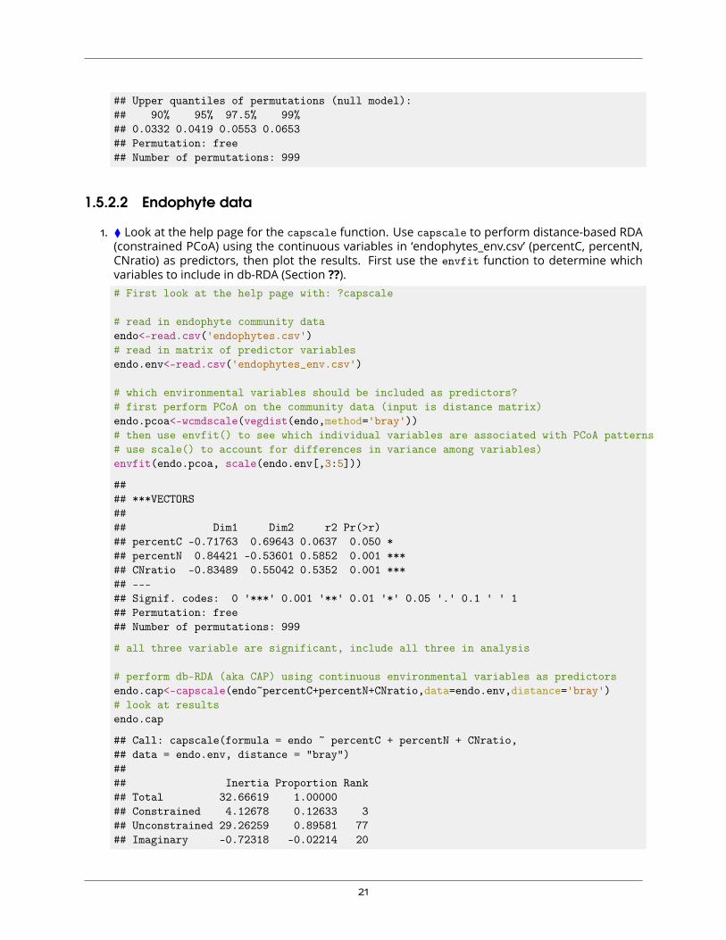
1. ⧫ Look at the help page for the capscale function. Use capscale to perform distance-based RDA(constrained PCoA) using the continuous variables in ‘endophytes_env.csv’ (percentC, percentN,CNratio) as predictors, then plot the results. First use the envfit function to determine whichvariables to include in db-RDA (Section ??).# First look at the help page with: ?capscale
# read in endophyte community dataendo<-read.csv('endophytes.csv')# read in matrix of predictor variablesendo.env<-read.csv('endophytes_env.csv')
# which environmental variables should be included as predictors?# first perform PCoA on the community data (input is distance matrix)endo.pcoa<-wcmdscale(vegdist(endo,method='bray'))# then use envfit() to see which individual variables are associated with PCoA patterns# use scale() to account for differences in variance among variables)envfit(endo.pcoa, scale(endo.env[,3:5]))
#### ***VECTORS#### Dim1 Dim2 r2 Pr(>r)## percentC -0.71763 0.69643 0.0637 0.050 *## percentN 0.84421 -0.53601 0.5852 0.001 ***## CNratio -0.83489 0.55042 0.5352 0.001 ***## ---## Signif. codes: 0 '***' 0.001 '**' 0.01 '*' 0.05 '.' 0.1 ' ' 1## Permutation: free## Number of permutations: 999
# all three variable are significant, include all three in analysis
# perform db-RDA (aka CAP) using continuous environmental variables as predictorsendo.cap<-capscale(endo~percentC+percentN+CNratio,data=endo.env,distance='bray')# look at resultsendo.cap
## Call: capscale(formula = endo ~ percentC + percentN + CNratio,## data = endo.env, distance = "bray")#### Inertia Proportion Rank## Total 32.66619 1.00000## Constrained 4.12678 0.12633 3## Unconstrained 29.26259 0.89581 77## Imaginary -0.72318 -0.02214 20
21
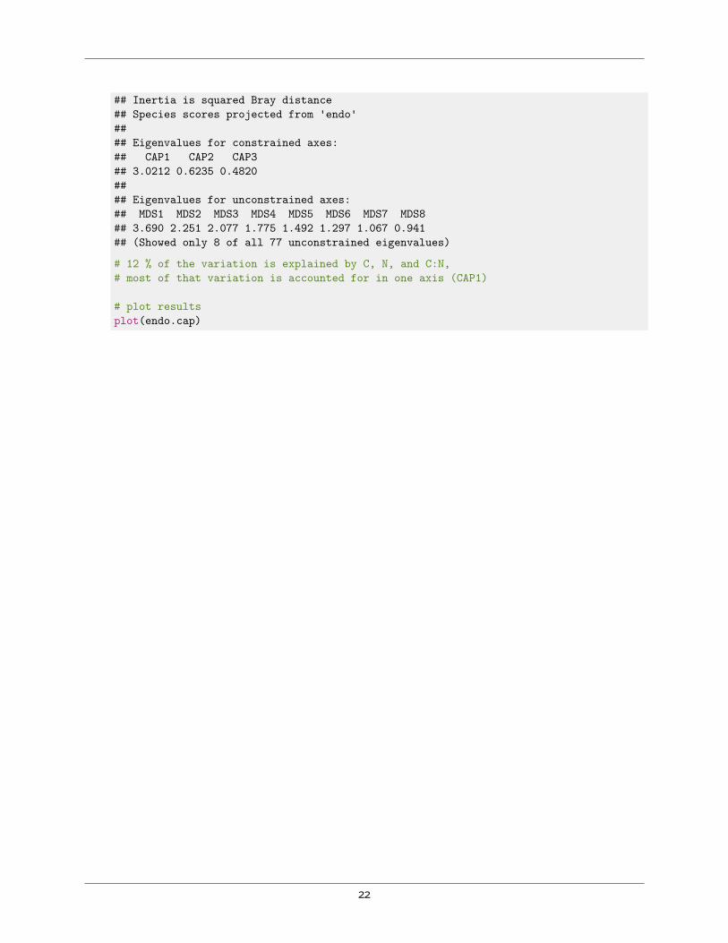
## Inertia is squared Bray distance## Species scores projected from 'endo'#### Eigenvalues for constrained axes:## CAP1 CAP2 CAP3## 3.0212 0.6235 0.4820#### Eigenvalues for unconstrained axes:## MDS1 MDS2 MDS3 MDS4 MDS5 MDS6 MDS7 MDS8## 3.690 2.251 2.077 1.775 1.492 1.297 1.067 0.941## (Showed only 8 of all 77 unconstrained eigenvalues)
# 12 % of the variation is explained by C, N, and C:N,# most of that variation is accounted for in one axis (CAP1)
# plot resultsplot(endo.cap)
22

−3 −2 −1 0 1 2 3
−3
−2
−1
01
2
CAP1
CA
P2 +++++++++ +++++
+++++++
+++++++
+
+++++++++++++++ ++
+
++++++++++ ++++ +
+++++++++++++++++++ ++++++++++++++++++++++++++++++++++++++++++++++++++++++++++
++++
+++++++++++
+ +++++++ ++++
++++++++++++++++++++++++
+
+ ++++++++++++++++++++++++++++++++++++++++++ +++++ ++++++
+
++++++++++++++ ++
++++++ ++++++++++++++++++++++++++
+
++++++++++++++++++++++ ++++++++++++++++++
++++++++++++
+ ++ +
+++++++ +++ +++++ ++++ ++++++
++++++++++++++++++++++++++++++++++++++++++++++++++++++++++++++++++++++++++++++++++ +++++++++++++++++++++++++
+++++++++++++++++++++++ +++++++++ ++++++++++
+
++++++++++++++++++++++++ +++++++++++++++++++++++++++++ +++++
+++ +++++
+
++ +++++++++
+ ++++++++++++++++++ ++++++++++++++++++++
++++++++++++++++++++++++++++++ ++++++ +
++++++++++++++++++
+++++++++++++++
+++ ++++++++ +
+
++++++
+++
++++ ++++++++++++++++++ +++++++++++++++
+
++++++++++++++
+++++++++++++++++++++++++++++++++++++++++++++++++++++++++++++++++++++++++++++++++++++++
percentC
percentN CNratio
# N and C:N are strongly collinear,# C is separated out along the second CAP axis
2. ⧫ Repeat the analysis in the previous exercise but use the ordistep function to determine whichvariables to include in db-RDA.# First look at the help page with: ?capscale
# read in endophyte community dataendo<-read.csv('endophytes.csv')# read in matrix of predictor variablesendo.env<-read.csv('endophytes_env.csv')# scale continuous variables so variance standardisedendo.env.std <- decostand(endo.env[, 3:5], method='standardize')
# which environmental variables should be included as predictors?# first perform CAP with each of the environmental variables
23
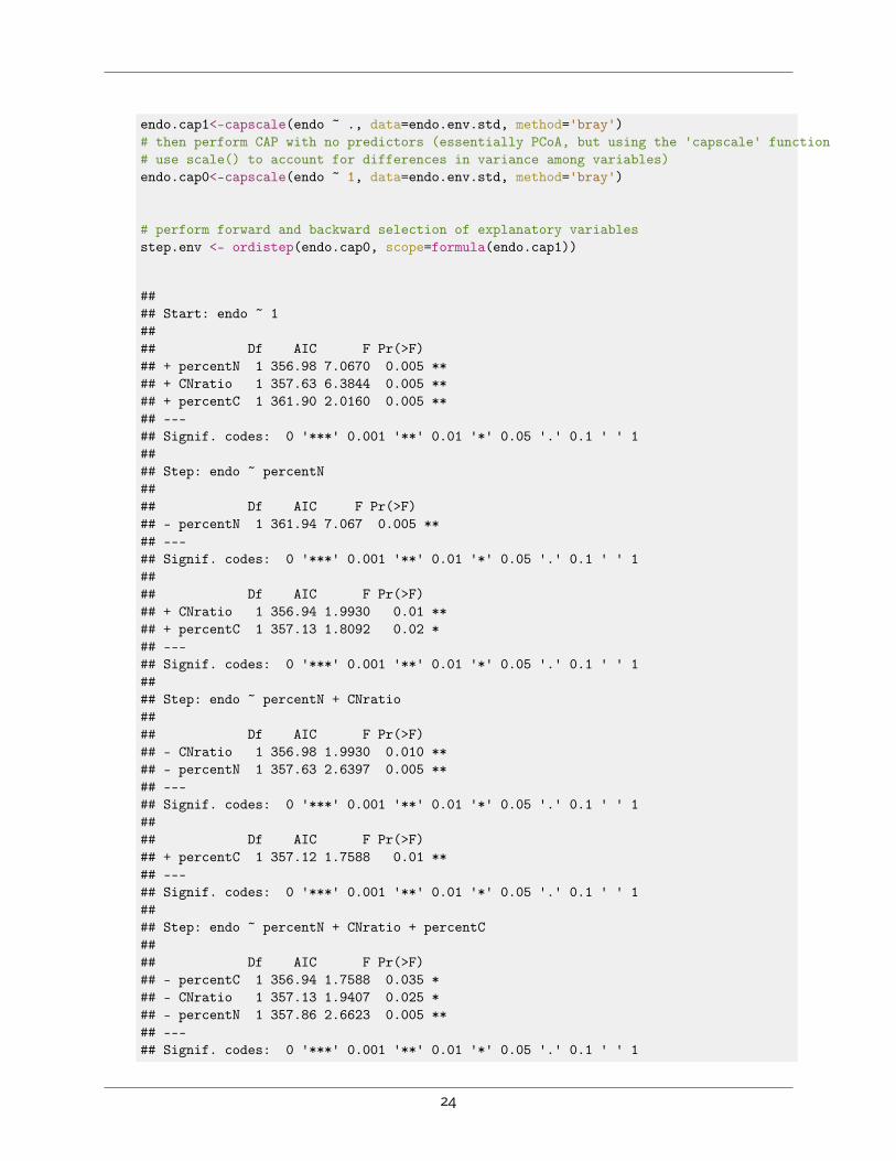
endo.cap1<-capscale(endo ~ ., data=endo.env.std, method='bray')# then perform CAP with no predictors (essentially PCoA, but using the 'capscale' function# use scale() to account for differences in variance among variables)endo.cap0<-capscale(endo ~ 1, data=endo.env.std, method='bray')
# perform forward and backward selection of explanatory variablesstep.env <- ordistep(endo.cap0, scope=formula(endo.cap1))
#### Start: endo ~ 1#### Df AIC F Pr(>F)## + percentN 1 356.98 7.0670 0.005 **## + CNratio 1 357.63 6.3844 0.005 **## + percentC 1 361.90 2.0160 0.005 **## ---## Signif. codes: 0 '***' 0.001 '**' 0.01 '*' 0.05 '.' 0.1 ' ' 1#### Step: endo ~ percentN#### Df AIC F Pr(>F)## - percentN 1 361.94 7.067 0.005 **## ---## Signif. codes: 0 '***' 0.001 '**' 0.01 '*' 0.05 '.' 0.1 ' ' 1#### Df AIC F Pr(>F)## + CNratio 1 356.94 1.9930 0.01 **## + percentC 1 357.13 1.8092 0.02 *## ---## Signif. codes: 0 '***' 0.001 '**' 0.01 '*' 0.05 '.' 0.1 ' ' 1#### Step: endo ~ percentN + CNratio#### Df AIC F Pr(>F)## - CNratio 1 356.98 1.9930 0.010 **## - percentN 1 357.63 2.6397 0.005 **## ---## Signif. codes: 0 '***' 0.001 '**' 0.01 '*' 0.05 '.' 0.1 ' ' 1#### Df AIC F Pr(>F)## + percentC 1 357.12 1.7588 0.01 **## ---## Signif. codes: 0 '***' 0.001 '**' 0.01 '*' 0.05 '.' 0.1 ' ' 1#### Step: endo ~ percentN + CNratio + percentC#### Df AIC F Pr(>F)## - percentC 1 356.94 1.7588 0.035 *## - CNratio 1 357.13 1.9407 0.025 *## - percentN 1 357.86 2.6623 0.005 **## ---## Signif. codes: 0 '***' 0.001 '**' 0.01 '*' 0.05 '.' 0.1 ' ' 1
24
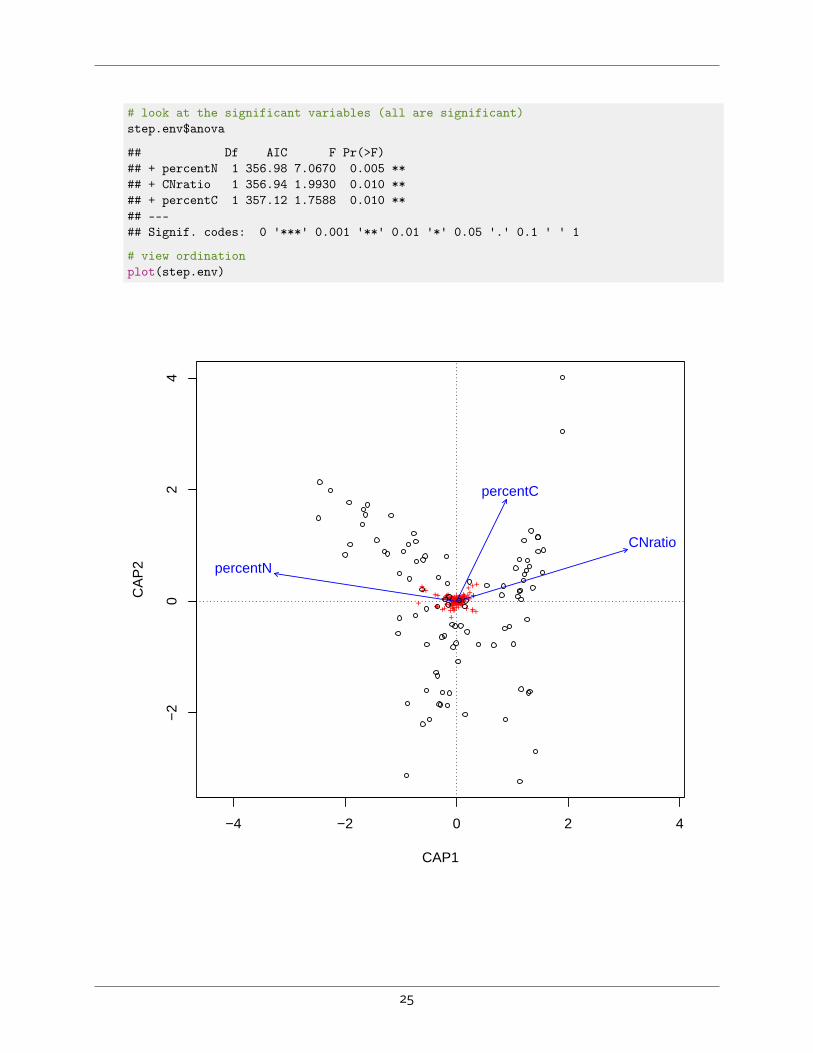
# look at the significant variables (all are significant)step.env$anova
## Df AIC F Pr(>F)## + percentN 1 356.98 7.0670 0.005 **## + CNratio 1 356.94 1.9930 0.010 **## + percentC 1 357.12 1.7588 0.010 **## ---## Signif. codes: 0 '***' 0.001 '**' 0.01 '*' 0.05 '.' 0.1 ' ' 1
# view ordinationplot(step.env)
−4 −2 0 2 4
−2
02
4
CAP1
CA
P2
+++++++++ +++++++++++++++++++
++++++++++++++++++
+
+++++++++++++++++++++++++++++++++++++++++++++++++++++++++++++++++++++++++++++++++++++++++++++
++++++++++++++
+ ++++++++++ +++
+++++++++++++++++++++++
+ ++++++++++++++++++++++++++++++++++++++++++ +++++ +++++++
+++++++++++++
+ ++++++++ ++++++++
++++++++++++++++++
+
++++++++++++++++++++++++++++++++++++++++
++++++++++++++
+ +++++++
+ ++++++++++++++++++++++++++++++++++++++++++++++++++++++++++++++++++++++++++++++++++++++++++++++++++++ ++++++++++++++++++++++++
++++++++++++++++++++++++ +++++++++++++++++++
+
+++++++++++++++++++++++++++++++++++++++++++++++++++++ +++++
+++ ++++++
+ ++++++++++
+++++++++++++++++++++++++++++++++++++++++++++++++++++++++++++++++++++ +++++++
++++++++++++++++++
++++++++++++++++++++++++++ +
++++++
++++++++++++++++++++++++++ +++++++++++++++
+
+++++++++++++++++++++++++++++++++++++++++++++++++++++++++++++++++++++++++++++++++++++++++++++++++++++
percentN
CNratio
percentC
25

1.5.3 Analysis of Structure 2: variation partitioning
1.5.3.1 Endophyte data
1. ⧫ Perform variation partitioning to determine whether leaf species, leaf chemistry, or sample typeexplains the most variation in fungal community composition.# load the vegan librarylibrary(vegan)
# read in tables containing species, and environmental variablesendo.spp <- read.csv('endophytes.csv') # column names represent OTUsendo.env <- read.csv('endophytes_env.csv')
dim(endo.spp)
## [1] 98 874
str(endo.env)
## 'data.frame': 98 obs. of 5 variables:## $ species : Factor w/ 9 levels "cladocalyx","crebra",..: 1 1 1 1 1 1 1 1 2 2 ...## $ type : Factor w/ 2 levels "fresh","litter": 1 2 1 2 1 2 1 1 1 2 ...## $ percentC: num 51.3 53 53.9 54.2 55.4 ...## $ percentN: num 2.271 1.212 1.508 0.892 1.916 ...## $ CNratio : num 22.6 43.7 35.7 60.8 28.9 ...
# select particular variables to proceed with (here we use both forward and backward selection but could use either one separately)
# set up the analysis with all predictorscap.env <- capscale(endo.spp ~ ., data=endo.env, distance='bray')
# set up the null cases with no predictorsmod0.env <- capscale(endo.spp ~ 1, data=endo.env, distance='bray')
# select variables in each predictor tablestep.env <- ordistep(mod0.env, scope=formula(cap.env))
#### Start: endo.spp ~ 1#### Df AIC F Pr(>F)## + species 8 333.93 3.5096 0.005 **## + type 1 335.96 11.2356 0.005 **## + percentN 1 337.81 9.2277 0.005 **## + CNratio 1 338.36 8.6318 0.005 **## + percentC 1 344.62 2.1608 0.010 **## ---## Signif. codes: 0 '***' 0.001 '**' 0.01 '*' 0.05 '.' 0.1 ' ' 1#### Step: endo.spp ~ species#### Df AIC F Pr(>F)## - species 8 344.8 3.5096 0.005 **## ---## Signif. codes: 0 '***' 0.001 '**' 0.01 '*' 0.05 '.' 0.1 ' ' 1
26
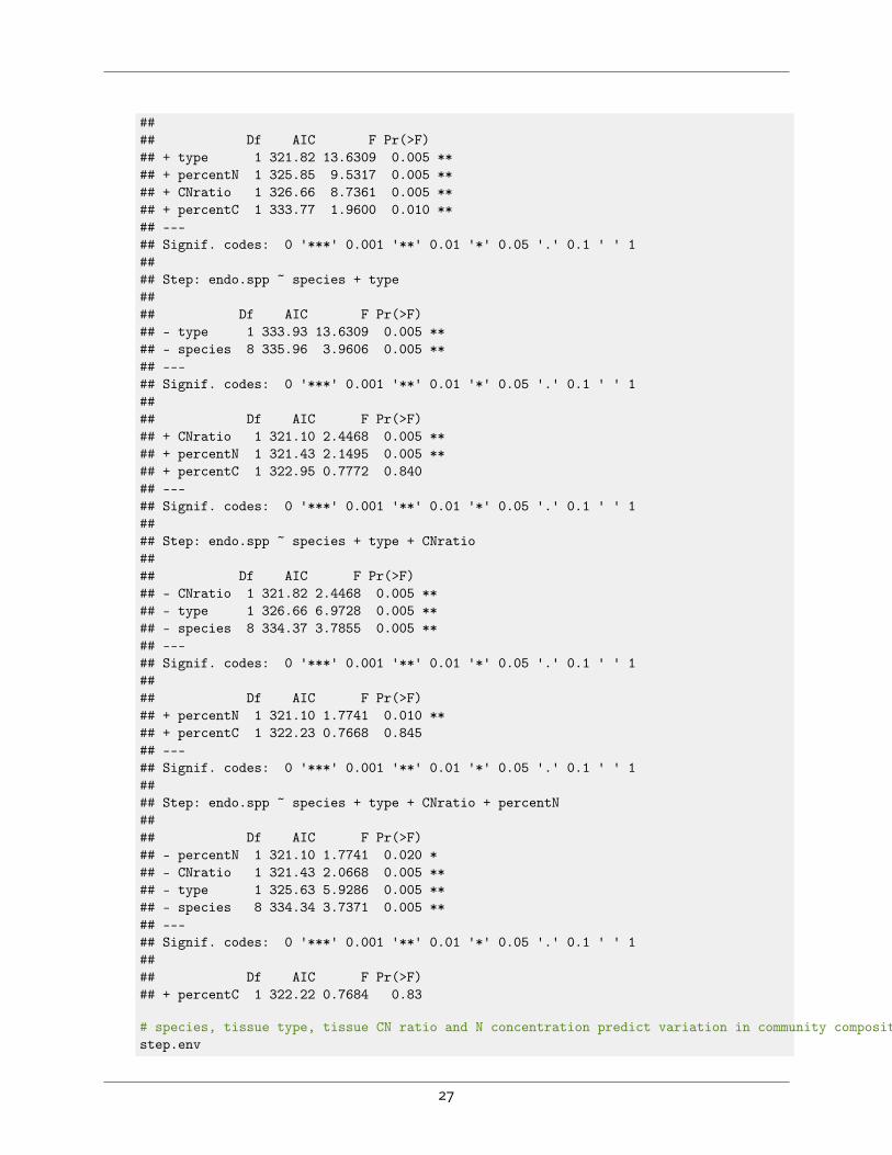
#### Df AIC F Pr(>F)## + type 1 321.82 13.6309 0.005 **## + percentN 1 325.85 9.5317 0.005 **## + CNratio 1 326.66 8.7361 0.005 **## + percentC 1 333.77 1.9600 0.010 **## ---## Signif. codes: 0 '***' 0.001 '**' 0.01 '*' 0.05 '.' 0.1 ' ' 1#### Step: endo.spp ~ species + type#### Df AIC F Pr(>F)## - type 1 333.93 13.6309 0.005 **## - species 8 335.96 3.9606 0.005 **## ---## Signif. codes: 0 '***' 0.001 '**' 0.01 '*' 0.05 '.' 0.1 ' ' 1#### Df AIC F Pr(>F)## + CNratio 1 321.10 2.4468 0.005 **## + percentN 1 321.43 2.1495 0.005 **## + percentC 1 322.95 0.7772 0.840## ---## Signif. codes: 0 '***' 0.001 '**' 0.01 '*' 0.05 '.' 0.1 ' ' 1#### Step: endo.spp ~ species + type + CNratio#### Df AIC F Pr(>F)## - CNratio 1 321.82 2.4468 0.005 **## - type 1 326.66 6.9728 0.005 **## - species 8 334.37 3.7855 0.005 **## ---## Signif. codes: 0 '***' 0.001 '**' 0.01 '*' 0.05 '.' 0.1 ' ' 1#### Df AIC F Pr(>F)## + percentN 1 321.10 1.7741 0.010 **## + percentC 1 322.23 0.7668 0.845## ---## Signif. codes: 0 '***' 0.001 '**' 0.01 '*' 0.05 '.' 0.1 ' ' 1#### Step: endo.spp ~ species + type + CNratio + percentN#### Df AIC F Pr(>F)## - percentN 1 321.10 1.7741 0.020 *## - CNratio 1 321.43 2.0668 0.005 **## - type 1 325.63 5.9286 0.005 **## - species 8 334.34 3.7371 0.005 **## ---## Signif. codes: 0 '***' 0.001 '**' 0.01 '*' 0.05 '.' 0.1 ' ' 1#### Df AIC F Pr(>F)## + percentC 1 322.22 0.7684 0.83
# species, tissue type, tissue CN ratio and N concentration predict variation in community compositionstep.env
27
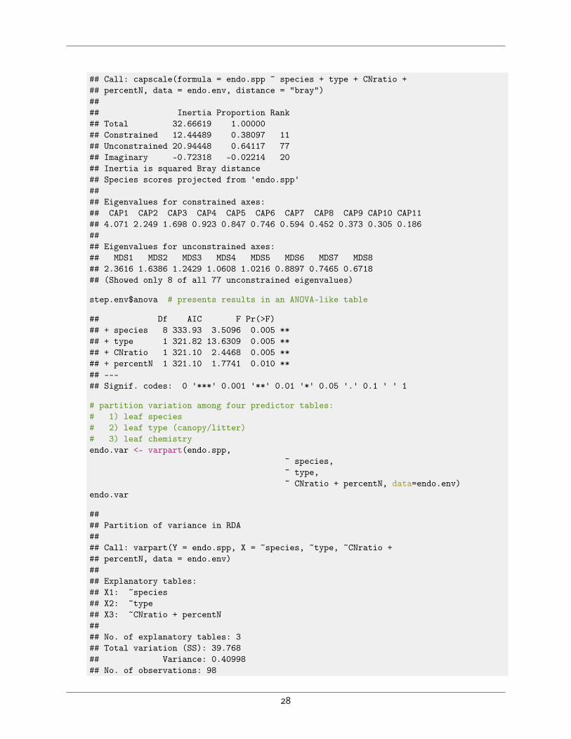
## Call: capscale(formula = endo.spp ~ species + type + CNratio +## percentN, data = endo.env, distance = "bray")#### Inertia Proportion Rank## Total 32.66619 1.00000## Constrained 12.44489 0.38097 11## Unconstrained 20.94448 0.64117 77## Imaginary -0.72318 -0.02214 20## Inertia is squared Bray distance## Species scores projected from 'endo.spp'#### Eigenvalues for constrained axes:## CAP1 CAP2 CAP3 CAP4 CAP5 CAP6 CAP7 CAP8 CAP9 CAP10 CAP11## 4.071 2.249 1.698 0.923 0.847 0.746 0.594 0.452 0.373 0.305 0.186#### Eigenvalues for unconstrained axes:## MDS1 MDS2 MDS3 MDS4 MDS5 MDS6 MDS7 MDS8## 2.3616 1.6386 1.2429 1.0608 1.0216 0.8897 0.7465 0.6718## (Showed only 8 of all 77 unconstrained eigenvalues)
step.env$anova # presents results in an ANOVA-like table
## Df AIC F Pr(>F)## + species 8 333.93 3.5096 0.005 **## + type 1 321.82 13.6309 0.005 **## + CNratio 1 321.10 2.4468 0.005 **## + percentN 1 321.10 1.7741 0.010 **## ---## Signif. codes: 0 '***' 0.001 '**' 0.01 '*' 0.05 '.' 0.1 ' ' 1
# partition variation among four predictor tables:# 1) leaf species# 2) leaf type (canopy/litter)# 3) leaf chemistryendo.var <- varpart(endo.spp,
~ species,~ type,~ CNratio + percentN, data=endo.env)
endo.var
#### Partition of variance in RDA#### Call: varpart(Y = endo.spp, X = ~species, ~type, ~CNratio +## percentN, data = endo.env)#### Explanatory tables:## X1: ~species## X2: ~type## X3: ~CNratio + percentN#### No. of explanatory tables: 3## Total variation (SS): 39.768## Variance: 0.40998## No. of observations: 98
28
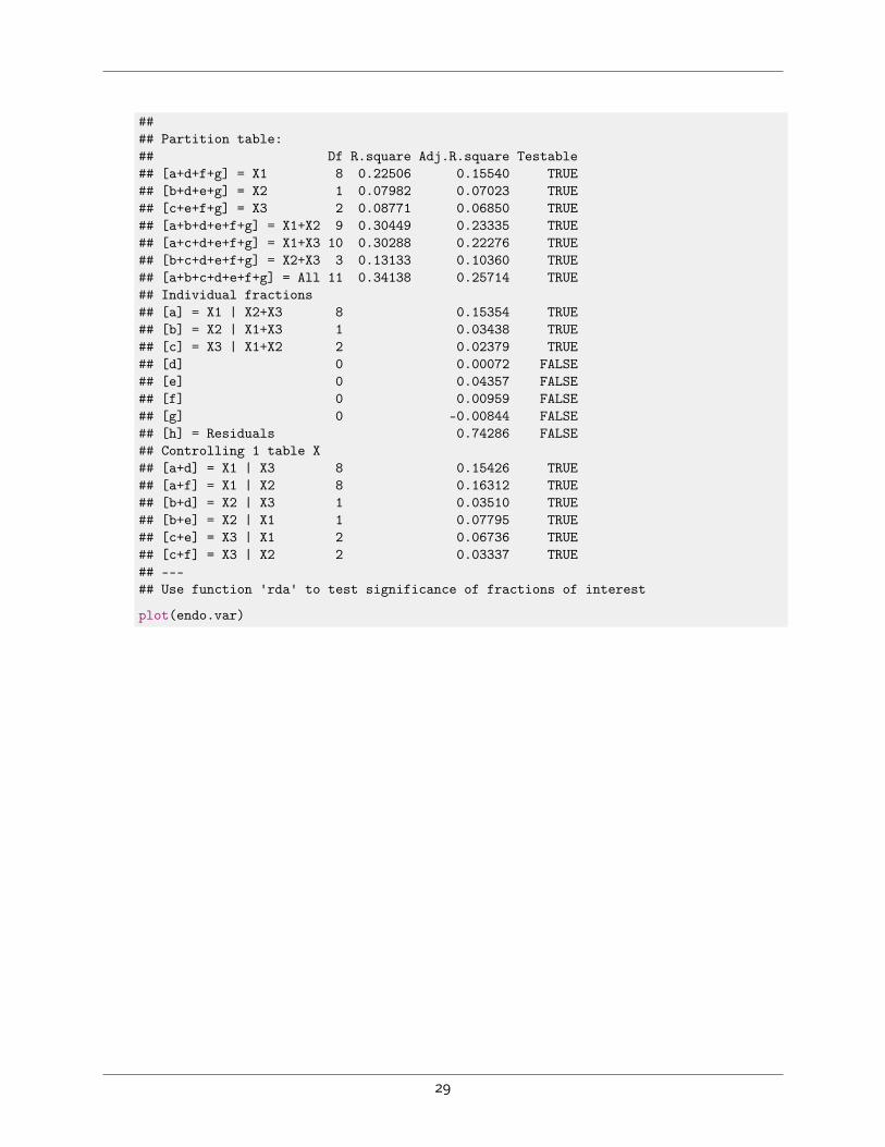
#### Partition table:## Df R.square Adj.R.square Testable## [a+d+f+g] = X1 8 0.22506 0.15540 TRUE## [b+d+e+g] = X2 1 0.07982 0.07023 TRUE## [c+e+f+g] = X3 2 0.08771 0.06850 TRUE## [a+b+d+e+f+g] = X1+X2 9 0.30449 0.23335 TRUE## [a+c+d+e+f+g] = X1+X3 10 0.30288 0.22276 TRUE## [b+c+d+e+f+g] = X2+X3 3 0.13133 0.10360 TRUE## [a+b+c+d+e+f+g] = All 11 0.34138 0.25714 TRUE## Individual fractions## [a] = X1 | X2+X3 8 0.15354 TRUE## [b] = X2 | X1+X3 1 0.03438 TRUE## [c] = X3 | X1+X2 2 0.02379 TRUE## [d] 0 0.00072 FALSE## [e] 0 0.04357 FALSE## [f] 0 0.00959 FALSE## [g] 0 -0.00844 FALSE## [h] = Residuals 0.74286 FALSE## Controlling 1 table X## [a+d] = X1 | X3 8 0.15426 TRUE## [a+f] = X1 | X2 8 0.16312 TRUE## [b+d] = X2 | X3 1 0.03510 TRUE## [b+e] = X2 | X1 1 0.07795 TRUE## [c+e] = X3 | X1 2 0.06736 TRUE## [c+f] = X3 | X2 2 0.03337 TRUE## ---## Use function 'rda' to test significance of fractions of interest
plot(endo.var)
29
X1 X2
X3
0.15 0.03
0.02
0.00
0.040.01
Residuals = 0.74
Values <0 not shown
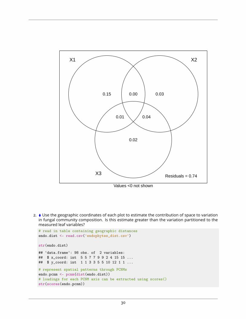
2. ⧫ Use the geographic coordinates of each plot to estimate the contribution of space to variationin fungal community composition. Is this estimate greater than the variation partitioned to themeasured leaf variables?# read in table containing geographic distancesendo.dist <- read.csv('endophytes_dist.csv')
str(endo.dist)
## 'data.frame': 98 obs. of 2 variables:## $ x_coord: int 5 5 7 7 9 9 2 4 15 15 ...## $ y_coord: int 1 1 3 3 5 5 10 12 1 1 ...
# represent spatial patterns through PCNMsendo.pcnm <- pcnm(dist(endo.dist))# loadings for each PCNM axis can be extracted using scores()str(scores(endo.pcnm))
30

## num [1:98, 1:19] -0.0454 -0.0454 -0.051 -0.051 -0.0588 ...## - attr(*, "dimnames")=List of 2## ..$ : chr [1:98] "1" "2" "3" "4" ...## ..$ : chr [1:19] "PCNM1" "PCNM2" "PCNM3" "PCNM4" ...
# select particular variables to proceed with (here we use both forward and backward selection but could use either one separately)
# set up the analysis with all predictorscap.pcnm <- capscale(endo.spp ~ ., data=as.data.frame(scores(endo.pcnm)), distance='bray')
# set up the null cases with no predictorsmod0.pcnm <- capscale(endo.spp ~ 1, data=as.data.frame(scores(endo.pcnm)), distance='bray')
# select variables in each predictor tablestep.pcnm <- ordistep(mod0.pcnm, scope=formula(cap.pcnm))
#### Start: endo.spp ~ 1#### Df AIC F Pr(>F)## + PCNM1 1 343.98 2.8088 0.005 **## + PCNM6 1 344.49 2.2910 0.005 **## + PCNM2 1 344.82 1.9586 0.020 *## + PCNM14 1 345.01 1.7723 0.025 *## + PCNM4 1 344.95 1.8274 0.030 *## + PCNM3 1 345.09 1.6890 0.040 *## + PCNM11 1 345.39 1.3937 0.100 .## + PCNM16 1 345.62 1.1661 0.235## + PCNM15 1 345.85 0.9413 0.520## + PCNM8 1 345.85 0.9408 0.580## + PCNM9 1 345.95 0.8402 0.670## + PCNM12 1 345.96 0.8319 0.670## + PCNM5 1 345.95 0.8414 0.725## + PCNM17 1 346.06 0.7343 0.840## + PCNM19 1 346.08 0.7088 0.845## + PCNM10 1 346.10 0.6862 0.875## + PCNM7 1 346.21 0.5831 0.970## + PCNM13 1 346.27 0.5225 0.990## + PCNM18 1 346.45 0.3468 1.000## ---## Signif. codes: 0 '***' 0.001 '**' 0.01 '*' 0.05 '.' 0.1 ' ' 1#### Step: endo.spp ~ PCNM1#### Df AIC F Pr(>F)## - PCNM1 1 344.8 2.8088 0.005 **## ---## Signif. codes: 0 '***' 0.001 '**' 0.01 '*' 0.05 '.' 0.1 ' ' 1#### Df AIC F Pr(>F)## + PCNM6 1 343.60 2.3351 0.005 **## + PCNM3 1 344.22 1.7212 0.010 **## + PCNM2 1 343.94 1.9961 0.015 *## + PCNM14 1 344.13 1.8062 0.035 *
31
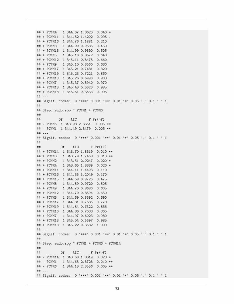
## + PCNM4 1 344.07 1.8623 0.040 *## + PCNM11 1 344.52 1.4202 0.095 .## + PCNM16 1 344.76 1.1881 0.210## + PCNM8 1 344.99 0.9585 0.450## + PCNM15 1 344.99 0.9590 0.505## + PCNM5 1 345.10 0.8572 0.640## + PCNM12 1 345.11 0.8475 0.660## + PCNM9 1 345.10 0.8560 0.680## + PCNM17 1 345.21 0.7481 0.820## + PCNM19 1 345.23 0.7221 0.860## + PCNM10 1 345.26 0.6990 0.900## + PCNM7 1 345.37 0.5940 0.970## + PCNM13 1 345.43 0.5323 0.985## + PCNM18 1 345.61 0.3533 0.995## ---## Signif. codes: 0 '***' 0.001 '**' 0.01 '*' 0.05 '.' 0.1 ' ' 1#### Step: endo.spp ~ PCNM1 + PCNM6#### Df AIC F Pr(>F)## - PCNM6 1 343.98 2.3351 0.005 **## - PCNM1 1 344.49 2.8479 0.005 **## ---## Signif. codes: 0 '***' 0.001 '**' 0.01 '*' 0.05 '.' 0.1 ' ' 1#### Df AIC F Pr(>F)## + PCNM14 1 343.70 1.8319 0.010 **## + PCNM3 1 343.79 1.7458 0.010 **## + PCNM2 1 343.51 2.0247 0.020 *## + PCNM4 1 343.65 1.8889 0.020 *## + PCNM11 1 344.11 1.4403 0.110## + PCNM16 1 344.35 1.2049 0.170## + PCNM15 1 344.59 0.9725 0.475## + PCNM8 1 344.59 0.9720 0.505## + PCNM9 1 344.70 0.8680 0.605## + PCNM12 1 344.70 0.8594 0.650## + PCNM5 1 344.69 0.8692 0.690## + PCNM17 1 344.81 0.7585 0.770## + PCNM19 1 344.84 0.7322 0.835## + PCNM10 1 344.86 0.7088 0.865## + PCNM7 1 344.97 0.6023 0.980## + PCNM13 1 345.04 0.5397 0.985## + PCNM18 1 345.22 0.3582 1.000## ---## Signif. codes: 0 '***' 0.001 '**' 0.01 '*' 0.05 '.' 0.1 ' ' 1#### Step: endo.spp ~ PCNM1 + PCNM6 + PCNM14#### Df AIC F Pr(>F)## - PCNM14 1 343.60 1.8319 0.020 *## - PCNM1 1 344.65 2.8728 0.010 **## - PCNM6 1 344.13 2.3556 0.005 **## ---## Signif. codes: 0 '***' 0.001 '**' 0.01 '*' 0.05 '.' 0.1 ' ' 1
32
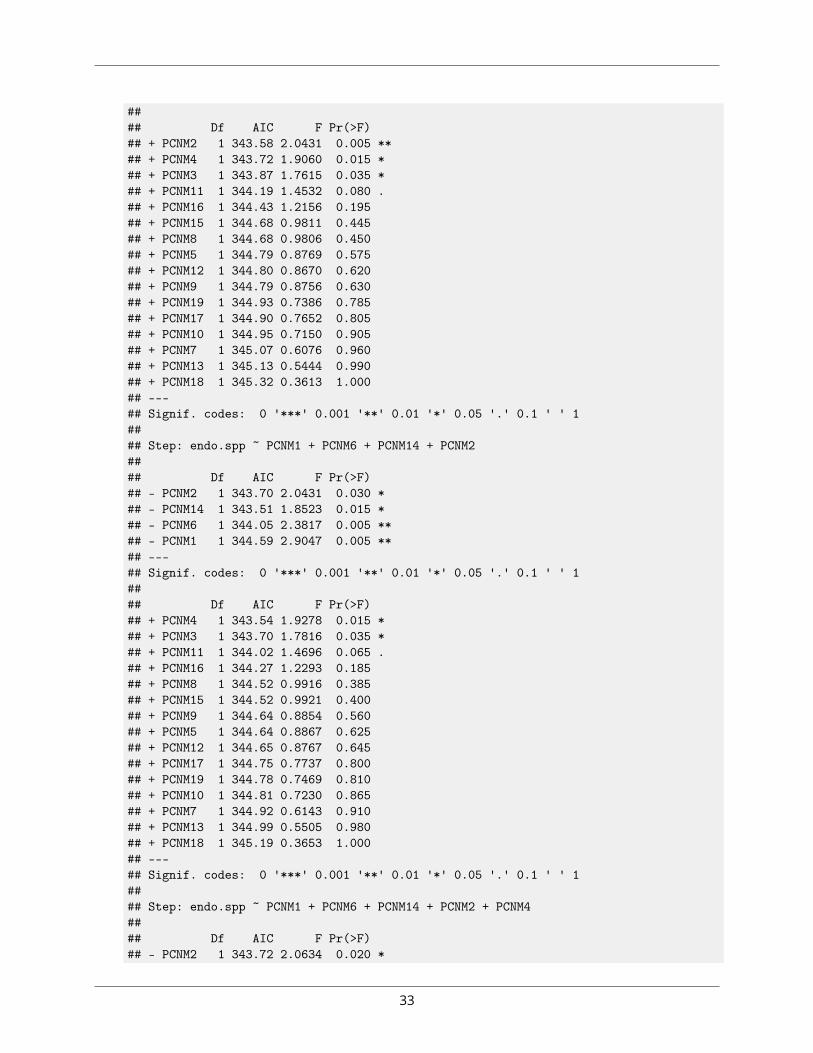
#### Df AIC F Pr(>F)## + PCNM2 1 343.58 2.0431 0.005 **## + PCNM4 1 343.72 1.9060 0.015 *## + PCNM3 1 343.87 1.7615 0.035 *## + PCNM11 1 344.19 1.4532 0.080 .## + PCNM16 1 344.43 1.2156 0.195## + PCNM15 1 344.68 0.9811 0.445## + PCNM8 1 344.68 0.9806 0.450## + PCNM5 1 344.79 0.8769 0.575## + PCNM12 1 344.80 0.8670 0.620## + PCNM9 1 344.79 0.8756 0.630## + PCNM19 1 344.93 0.7386 0.785## + PCNM17 1 344.90 0.7652 0.805## + PCNM10 1 344.95 0.7150 0.905## + PCNM7 1 345.07 0.6076 0.960## + PCNM13 1 345.13 0.5444 0.990## + PCNM18 1 345.32 0.3613 1.000## ---## Signif. codes: 0 '***' 0.001 '**' 0.01 '*' 0.05 '.' 0.1 ' ' 1#### Step: endo.spp ~ PCNM1 + PCNM6 + PCNM14 + PCNM2#### Df AIC F Pr(>F)## - PCNM2 1 343.70 2.0431 0.030 *## - PCNM14 1 343.51 1.8523 0.015 *## - PCNM6 1 344.05 2.3817 0.005 **## - PCNM1 1 344.59 2.9047 0.005 **## ---## Signif. codes: 0 '***' 0.001 '**' 0.01 '*' 0.05 '.' 0.1 ' ' 1#### Df AIC F Pr(>F)## + PCNM4 1 343.54 1.9278 0.015 *## + PCNM3 1 343.70 1.7816 0.035 *## + PCNM11 1 344.02 1.4696 0.065 .## + PCNM16 1 344.27 1.2293 0.185## + PCNM8 1 344.52 0.9916 0.385## + PCNM15 1 344.52 0.9921 0.400## + PCNM9 1 344.64 0.8854 0.560## + PCNM5 1 344.64 0.8867 0.625## + PCNM12 1 344.65 0.8767 0.645## + PCNM17 1 344.75 0.7737 0.800## + PCNM19 1 344.78 0.7469 0.810## + PCNM10 1 344.81 0.7230 0.865## + PCNM7 1 344.92 0.6143 0.910## + PCNM13 1 344.99 0.5505 0.980## + PCNM18 1 345.19 0.3653 1.000## ---## Signif. codes: 0 '***' 0.001 '**' 0.01 '*' 0.05 '.' 0.1 ' ' 1#### Step: endo.spp ~ PCNM1 + PCNM6 + PCNM14 + PCNM2 + PCNM4#### Df AIC F Pr(>F)## - PCNM2 1 343.72 2.0634 0.020 *
33
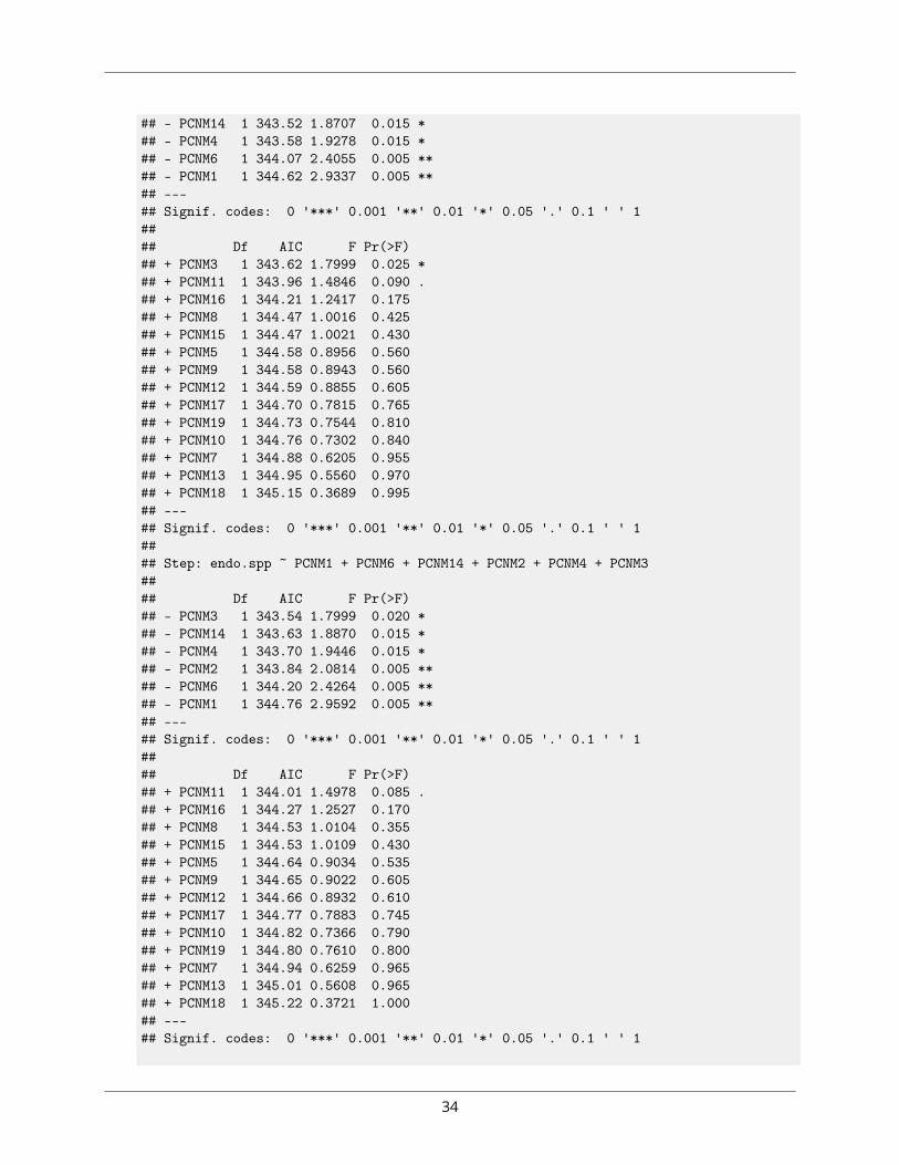
## - PCNM14 1 343.52 1.8707 0.015 *## - PCNM4 1 343.58 1.9278 0.015 *## - PCNM6 1 344.07 2.4055 0.005 **## - PCNM1 1 344.62 2.9337 0.005 **## ---## Signif. codes: 0 '***' 0.001 '**' 0.01 '*' 0.05 '.' 0.1 ' ' 1#### Df AIC F Pr(>F)## + PCNM3 1 343.62 1.7999 0.025 *## + PCNM11 1 343.96 1.4846 0.090 .## + PCNM16 1 344.21 1.2417 0.175## + PCNM8 1 344.47 1.0016 0.425## + PCNM15 1 344.47 1.0021 0.430## + PCNM5 1 344.58 0.8956 0.560## + PCNM9 1 344.58 0.8943 0.560## + PCNM12 1 344.59 0.8855 0.605## + PCNM17 1 344.70 0.7815 0.765## + PCNM19 1 344.73 0.7544 0.810## + PCNM10 1 344.76 0.7302 0.840## + PCNM7 1 344.88 0.6205 0.955## + PCNM13 1 344.95 0.5560 0.970## + PCNM18 1 345.15 0.3689 0.995## ---## Signif. codes: 0 '***' 0.001 '**' 0.01 '*' 0.05 '.' 0.1 ' ' 1#### Step: endo.spp ~ PCNM1 + PCNM6 + PCNM14 + PCNM2 + PCNM4 + PCNM3#### Df AIC F Pr(>F)## - PCNM3 1 343.54 1.7999 0.020 *## - PCNM14 1 343.63 1.8870 0.015 *## - PCNM4 1 343.70 1.9446 0.015 *## - PCNM2 1 343.84 2.0814 0.005 **## - PCNM6 1 344.20 2.4264 0.005 **## - PCNM1 1 344.76 2.9592 0.005 **## ---## Signif. codes: 0 '***' 0.001 '**' 0.01 '*' 0.05 '.' 0.1 ' ' 1#### Df AIC F Pr(>F)## + PCNM11 1 344.01 1.4978 0.085 .## + PCNM16 1 344.27 1.2527 0.170## + PCNM8 1 344.53 1.0104 0.355## + PCNM15 1 344.53 1.0109 0.430## + PCNM5 1 344.64 0.9034 0.535## + PCNM9 1 344.65 0.9022 0.605## + PCNM12 1 344.66 0.8932 0.610## + PCNM17 1 344.77 0.7883 0.745## + PCNM10 1 344.82 0.7366 0.790## + PCNM19 1 344.80 0.7610 0.800## + PCNM7 1 344.94 0.6259 0.965## + PCNM13 1 345.01 0.5608 0.965## + PCNM18 1 345.22 0.3721 1.000## ---## Signif. codes: 0 '***' 0.001 '**' 0.01 '*' 0.05 '.' 0.1 ' ' 1
34
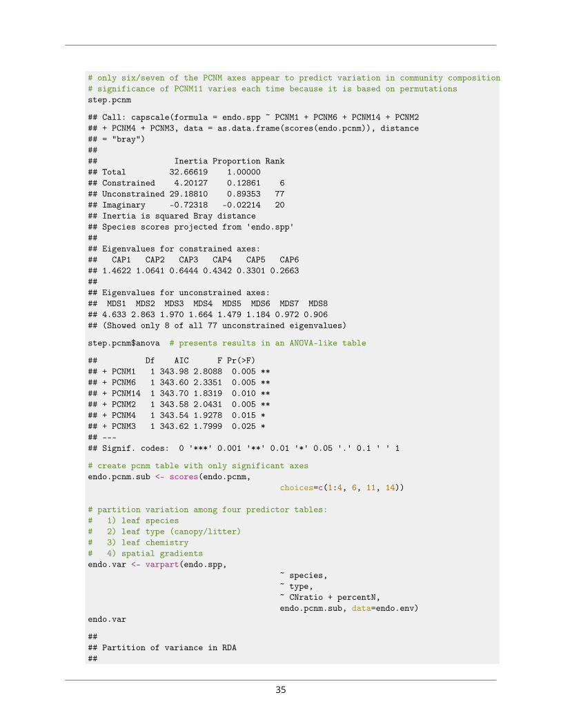
# only six/seven of the PCNM axes appear to predict variation in community composition# significance of PCNM11 varies each time because it is based on permutationsstep.pcnm
## Call: capscale(formula = endo.spp ~ PCNM1 + PCNM6 + PCNM14 + PCNM2## + PCNM4 + PCNM3, data = as.data.frame(scores(endo.pcnm)), distance## = "bray")#### Inertia Proportion Rank## Total 32.66619 1.00000## Constrained 4.20127 0.12861 6## Unconstrained 29.18810 0.89353 77## Imaginary -0.72318 -0.02214 20## Inertia is squared Bray distance## Species scores projected from 'endo.spp'#### Eigenvalues for constrained axes:## CAP1 CAP2 CAP3 CAP4 CAP5 CAP6## 1.4622 1.0641 0.6444 0.4342 0.3301 0.2663#### Eigenvalues for unconstrained axes:## MDS1 MDS2 MDS3 MDS4 MDS5 MDS6 MDS7 MDS8## 4.633 2.863 1.970 1.664 1.479 1.184 0.972 0.906## (Showed only 8 of all 77 unconstrained eigenvalues)
step.pcnm$anova # presents results in an ANOVA-like table
## Df AIC F Pr(>F)## + PCNM1 1 343.98 2.8088 0.005 **## + PCNM6 1 343.60 2.3351 0.005 **## + PCNM14 1 343.70 1.8319 0.010 **## + PCNM2 1 343.58 2.0431 0.005 **## + PCNM4 1 343.54 1.9278 0.015 *## + PCNM3 1 343.62 1.7999 0.025 *## ---## Signif. codes: 0 '***' 0.001 '**' 0.01 '*' 0.05 '.' 0.1 ' ' 1
# create pcnm table with only significant axesendo.pcnm.sub <- scores(endo.pcnm,
choices=c(1:4, 6, 11, 14))
# partition variation among four predictor tables:# 1) leaf species# 2) leaf type (canopy/litter)# 3) leaf chemistry# 4) spatial gradientsendo.var <- varpart(endo.spp,
~ species,~ type,~ CNratio + percentN,endo.pcnm.sub, data=endo.env)
endo.var
#### Partition of variance in RDA##
35
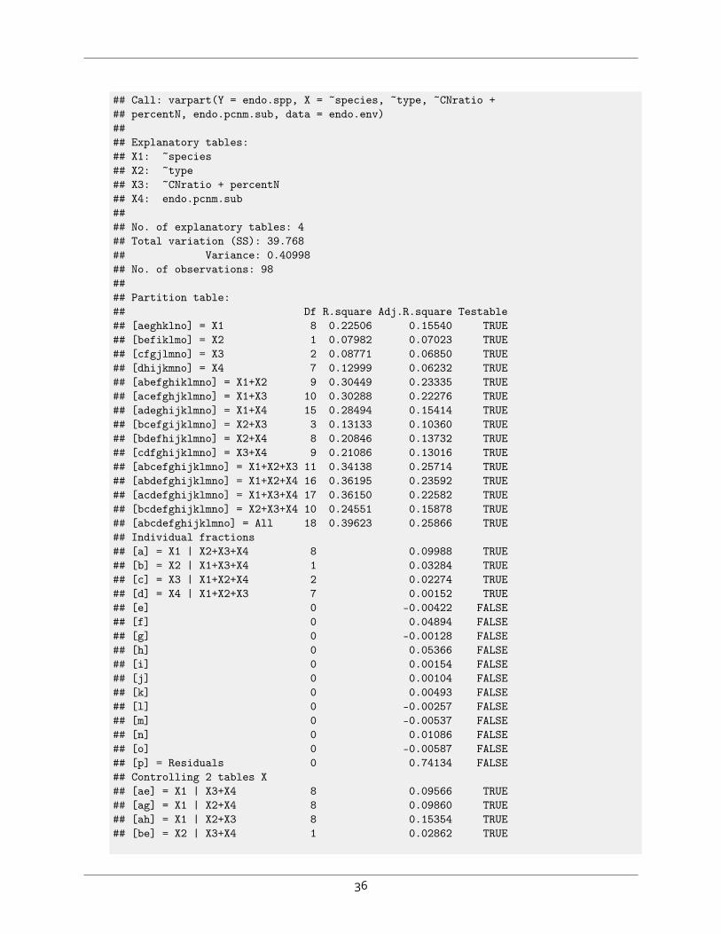
## Call: varpart(Y = endo.spp, X = ~species, ~type, ~CNratio +## percentN, endo.pcnm.sub, data = endo.env)#### Explanatory tables:## X1: ~species## X2: ~type## X3: ~CNratio + percentN## X4: endo.pcnm.sub#### No. of explanatory tables: 4## Total variation (SS): 39.768## Variance: 0.40998## No. of observations: 98#### Partition table:## Df R.square Adj.R.square Testable## [aeghklno] = X1 8 0.22506 0.15540 TRUE## [befiklmo] = X2 1 0.07982 0.07023 TRUE## [cfgjlmno] = X3 2 0.08771 0.06850 TRUE## [dhijkmno] = X4 7 0.12999 0.06232 TRUE## [abefghiklmno] = X1+X2 9 0.30449 0.23335 TRUE## [acefghjklmno] = X1+X3 10 0.30288 0.22276 TRUE## [adeghijklmno] = X1+X4 15 0.28494 0.15414 TRUE## [bcefgijklmno] = X2+X3 3 0.13133 0.10360 TRUE## [bdefhijklmno] = X2+X4 8 0.20846 0.13732 TRUE## [cdfghijklmno] = X3+X4 9 0.21086 0.13016 TRUE## [abcefghijklmno] = X1+X2+X3 11 0.34138 0.25714 TRUE## [abdefghijklmno] = X1+X2+X4 16 0.36195 0.23592 TRUE## [acdefghijklmno] = X1+X3+X4 17 0.36150 0.22582 TRUE## [bcdefghijklmno] = X2+X3+X4 10 0.24551 0.15878 TRUE## [abcdefghijklmno] = All 18 0.39623 0.25866 TRUE## Individual fractions## [a] = X1 | X2+X3+X4 8 0.09988 TRUE## [b] = X2 | X1+X3+X4 1 0.03284 TRUE## [c] = X3 | X1+X2+X4 2 0.02274 TRUE## [d] = X4 | X1+X2+X3 7 0.00152 TRUE## [e] 0 -0.00422 FALSE## [f] 0 0.04894 FALSE## [g] 0 -0.00128 FALSE## [h] 0 0.05366 FALSE## [i] 0 0.00154 FALSE## [j] 0 0.00104 FALSE## [k] 0 0.00493 FALSE## [l] 0 -0.00257 FALSE## [m] 0 -0.00537 FALSE## [n] 0 0.01086 FALSE## [o] 0 -0.00587 FALSE## [p] = Residuals 0 0.74134 FALSE## Controlling 2 tables X## [ae] = X1 | X3+X4 8 0.09566 TRUE## [ag] = X1 | X2+X4 8 0.09860 TRUE## [ah] = X1 | X2+X3 8 0.15354 TRUE## [be] = X2 | X3+X4 1 0.02862 TRUE
36
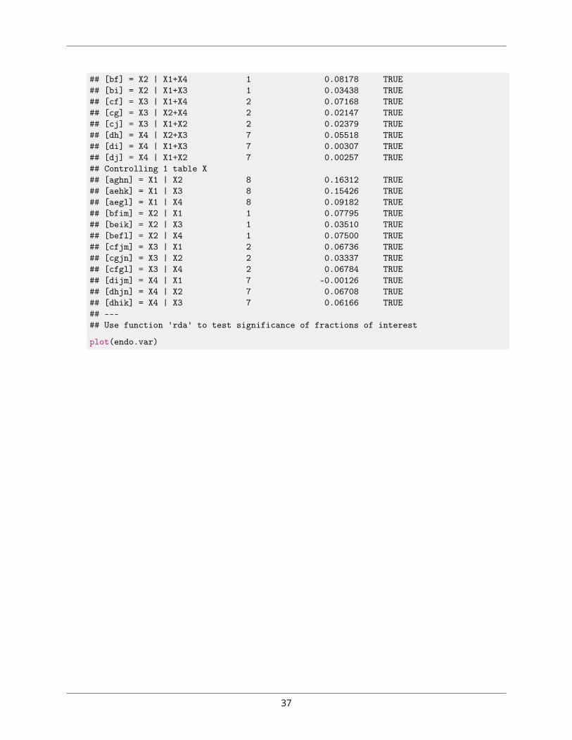
## [bf] = X2 | X1+X4 1 0.08178 TRUE## [bi] = X2 | X1+X3 1 0.03438 TRUE## [cf] = X3 | X1+X4 2 0.07168 TRUE## [cg] = X3 | X2+X4 2 0.02147 TRUE## [cj] = X3 | X1+X2 2 0.02379 TRUE## [dh] = X4 | X2+X3 7 0.05518 TRUE## [di] = X4 | X1+X3 7 0.00307 TRUE## [dj] = X4 | X1+X2 7 0.00257 TRUE## Controlling 1 table X## [aghn] = X1 | X2 8 0.16312 TRUE## [aehk] = X1 | X3 8 0.15426 TRUE## [aegl] = X1 | X4 8 0.09182 TRUE## [bfim] = X2 | X1 1 0.07795 TRUE## [beik] = X2 | X3 1 0.03510 TRUE## [befl] = X2 | X4 1 0.07500 TRUE## [cfjm] = X3 | X1 2 0.06736 TRUE## [cgjn] = X3 | X2 2 0.03337 TRUE## [cfgl] = X3 | X4 2 0.06784 TRUE## [dijm] = X4 | X1 7 -0.00126 TRUE## [dhjn] = X4 | X2 7 0.06708 TRUE## [dhik] = X4 | X3 7 0.06166 TRUE## ---## Use function 'rda' to test significance of fractions of interest
plot(endo.var)
37
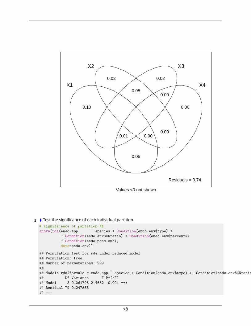
X1
X2 X3
X4
0.10
0.03 0.02
0.00
0.05
0.05
0.00
0.00
0.00
0.01
Residuals = 0.74
Values <0 not shown
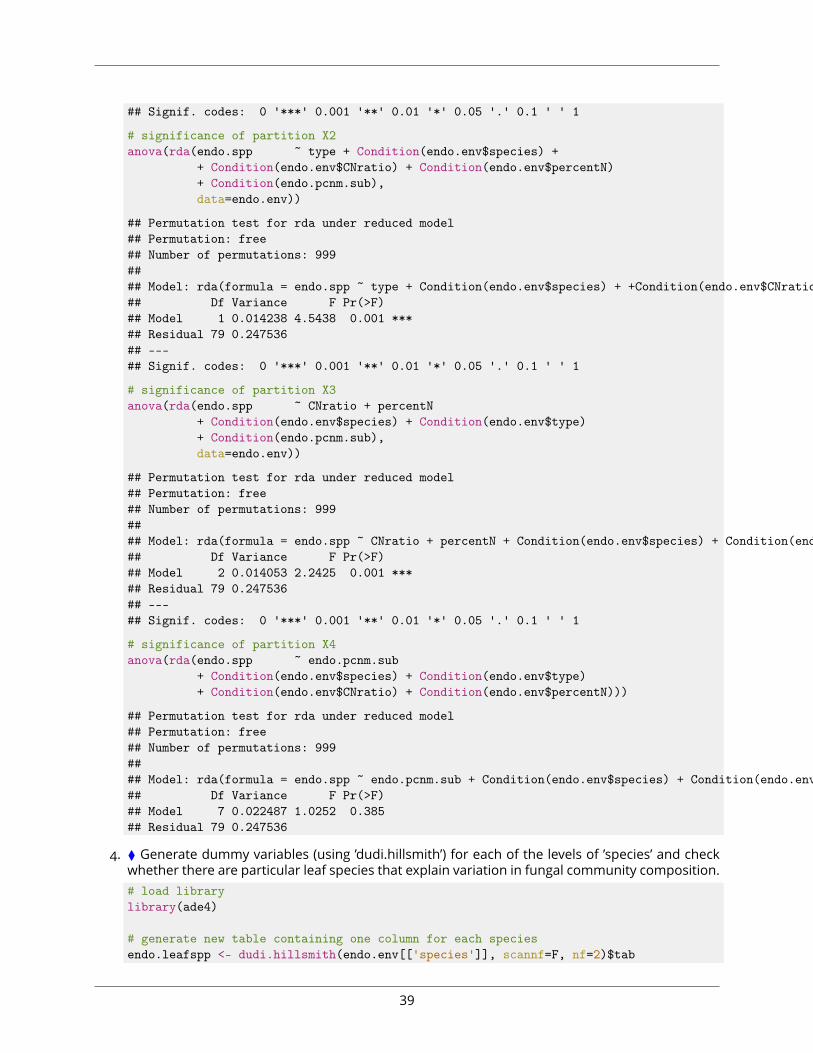
3. ⧫ Test the significance of each individual partition.# significance of partition X1anova(rda(endo.spp ~ species + Condition(endo.env$type) +
+ Condition(endo.env$CNratio) + Condition(endo.env$percentN)+ Condition(endo.pcnm.sub),data=endo.env))
## Permutation test for rda under reduced model## Permutation: free## Number of permutations: 999#### Model: rda(formula = endo.spp ~ species + Condition(endo.env$type) + +Condition(endo.env$CNratio) + Condition(endo.env$percentN) + Condition(endo.pcnm.sub), data = endo.env)## Df Variance F Pr(>F)## Model 8 0.061795 2.4652 0.001 ***## Residual 79 0.247536## ---
38
## Signif. codes: 0 '***' 0.001 '**' 0.01 '*' 0.05 '.' 0.1 ' ' 1
# significance of partition X2anova(rda(endo.spp ~ type + Condition(endo.env$species) +
+ Condition(endo.env$CNratio) + Condition(endo.env$percentN)+ Condition(endo.pcnm.sub),data=endo.env))
## Permutation test for rda under reduced model## Permutation: free## Number of permutations: 999#### Model: rda(formula = endo.spp ~ type + Condition(endo.env$species) + +Condition(endo.env$CNratio) + Condition(endo.env$percentN) + Condition(endo.pcnm.sub), data = endo.env)## Df Variance F Pr(>F)## Model 1 0.014238 4.5438 0.001 ***## Residual 79 0.247536## ---## Signif. codes: 0 '***' 0.001 '**' 0.01 '*' 0.05 '.' 0.1 ' ' 1
# significance of partition X3anova(rda(endo.spp ~ CNratio + percentN
+ Condition(endo.env$species) + Condition(endo.env$type)+ Condition(endo.pcnm.sub),data=endo.env))
## Permutation test for rda under reduced model## Permutation: free## Number of permutations: 999#### Model: rda(formula = endo.spp ~ CNratio + percentN + Condition(endo.env$species) + Condition(endo.env$type) + Condition(endo.pcnm.sub), data = endo.env)## Df Variance F Pr(>F)## Model 2 0.014053 2.2425 0.001 ***## Residual 79 0.247536## ---## Signif. codes: 0 '***' 0.001 '**' 0.01 '*' 0.05 '.' 0.1 ' ' 1
# significance of partition X4anova(rda(endo.spp ~ endo.pcnm.sub
+ Condition(endo.env$species) + Condition(endo.env$type)+ Condition(endo.env$CNratio) + Condition(endo.env$percentN)))
## Permutation test for rda under reduced model## Permutation: free## Number of permutations: 999#### Model: rda(formula = endo.spp ~ endo.pcnm.sub + Condition(endo.env$species) + Condition(endo.env$type) + Condition(endo.env$CNratio) + Condition(endo.env$percentN))## Df Variance F Pr(>F)## Model 7 0.022487 1.0252 0.385## Residual 79 0.247536
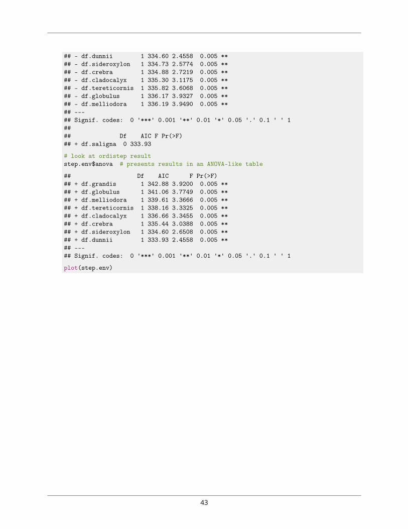
4. ⧫ Generate dummy variables (using ’dudi.hillsmith’) for each of the levels of ’species’ and checkwhether there are particular leaf species that explain variation in fungal community composition.# load librarylibrary(ade4)
# generate new table containing one column for each speciesendo.leafspp <- dudi.hillsmith(endo.env[['species']], scannf=F, nf=2)$tab
39
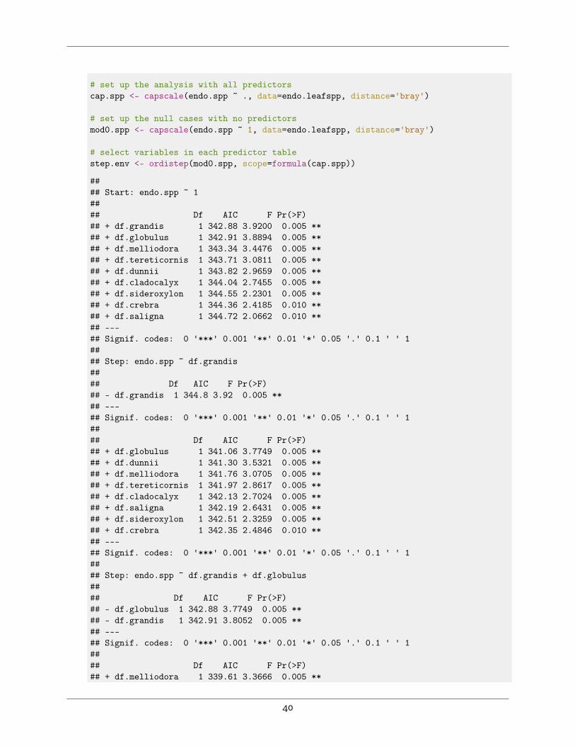
# set up the analysis with all predictorscap.spp <- capscale(endo.spp ~ ., data=endo.leafspp, distance='bray')
# set up the null cases with no predictorsmod0.spp <- capscale(endo.spp ~ 1, data=endo.leafspp, distance='bray')
# select variables in each predictor tablestep.env <- ordistep(mod0.spp, scope=formula(cap.spp))
#### Start: endo.spp ~ 1#### Df AIC F Pr(>F)## + df.grandis 1 342.88 3.9200 0.005 **## + df.globulus 1 342.91 3.8894 0.005 **## + df.melliodora 1 343.34 3.4476 0.005 **## + df.tereticornis 1 343.71 3.0811 0.005 **## + df.dunnii 1 343.82 2.9659 0.005 **## + df.cladocalyx 1 344.04 2.7455 0.005 **## + df.sideroxylon 1 344.55 2.2301 0.005 **## + df.crebra 1 344.36 2.4185 0.010 **## + df.saligna 1 344.72 2.0662 0.010 **## ---## Signif. codes: 0 '***' 0.001 '**' 0.01 '*' 0.05 '.' 0.1 ' ' 1#### Step: endo.spp ~ df.grandis#### Df AIC F Pr(>F)## - df.grandis 1 344.8 3.92 0.005 **## ---## Signif. codes: 0 '***' 0.001 '**' 0.01 '*' 0.05 '.' 0.1 ' ' 1#### Df AIC F Pr(>F)## + df.globulus 1 341.06 3.7749 0.005 **## + df.dunnii 1 341.30 3.5321 0.005 **## + df.melliodora 1 341.76 3.0705 0.005 **## + df.tereticornis 1 341.97 2.8617 0.005 **## + df.cladocalyx 1 342.13 2.7024 0.005 **## + df.saligna 1 342.19 2.6431 0.005 **## + df.sideroxylon 1 342.51 2.3259 0.005 **## + df.crebra 1 342.35 2.4846 0.010 **## ---## Signif. codes: 0 '***' 0.001 '**' 0.01 '*' 0.05 '.' 0.1 ' ' 1#### Step: endo.spp ~ df.grandis + df.globulus#### Df AIC F Pr(>F)## - df.globulus 1 342.88 3.7749 0.005 **## - df.grandis 1 342.91 3.8052 0.005 **## ---## Signif. codes: 0 '***' 0.001 '**' 0.01 '*' 0.05 '.' 0.1 ' ' 1#### Df AIC F Pr(>F)## + df.melliodora 1 339.61 3.3666 0.005 **
40
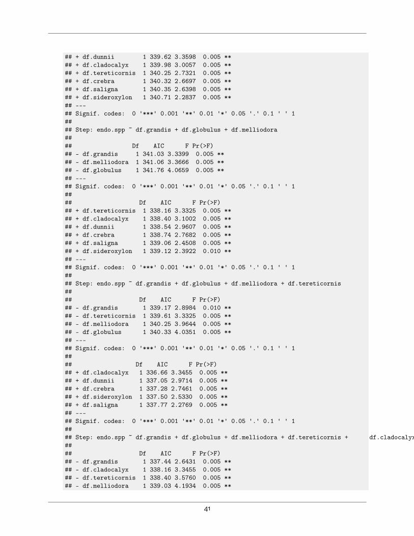
## + df.dunnii 1 339.62 3.3598 0.005 **## + df.cladocalyx 1 339.98 3.0057 0.005 **## + df.tereticornis 1 340.25 2.7321 0.005 **## + df.crebra 1 340.32 2.6697 0.005 **## + df.saligna 1 340.35 2.6398 0.005 **## + df.sideroxylon 1 340.71 2.2837 0.005 **## ---## Signif. codes: 0 '***' 0.001 '**' 0.01 '*' 0.05 '.' 0.1 ' ' 1#### Step: endo.spp ~ df.grandis + df.globulus + df.melliodora#### Df AIC F Pr(>F)## - df.grandis 1 341.03 3.3399 0.005 **## - df.melliodora 1 341.06 3.3666 0.005 **## - df.globulus 1 341.76 4.0659 0.005 **## ---## Signif. codes: 0 '***' 0.001 '**' 0.01 '*' 0.05 '.' 0.1 ' ' 1#### Df AIC F Pr(>F)## + df.tereticornis 1 338.16 3.3325 0.005 **## + df.cladocalyx 1 338.40 3.1002 0.005 **## + df.dunnii 1 338.54 2.9607 0.005 **## + df.crebra 1 338.74 2.7682 0.005 **## + df.saligna 1 339.06 2.4508 0.005 **## + df.sideroxylon 1 339.12 2.3922 0.010 **## ---## Signif. codes: 0 '***' 0.001 '**' 0.01 '*' 0.05 '.' 0.1 ' ' 1#### Step: endo.spp ~ df.grandis + df.globulus + df.melliodora + df.tereticornis#### Df AIC F Pr(>F)## - df.grandis 1 339.17 2.8984 0.010 **## - df.tereticornis 1 339.61 3.3325 0.005 **## - df.melliodora 1 340.25 3.9644 0.005 **## - df.globulus 1 340.33 4.0351 0.005 **## ---## Signif. codes: 0 '***' 0.001 '**' 0.01 '*' 0.05 '.' 0.1 ' ' 1#### Df AIC F Pr(>F)## + df.cladocalyx 1 336.66 3.3455 0.005 **## + df.dunnii 1 337.05 2.9714 0.005 **## + df.crebra 1 337.28 2.7461 0.005 **## + df.sideroxylon 1 337.50 2.5330 0.005 **## + df.saligna 1 337.77 2.2769 0.005 **## ---## Signif. codes: 0 '***' 0.001 '**' 0.01 '*' 0.05 '.' 0.1 ' ' 1#### Step: endo.spp ~ df.grandis + df.globulus + df.melliodora + df.tereticornis + df.cladocalyx#### Df AIC F Pr(>F)## - df.grandis 1 337.44 2.6431 0.005 **## - df.cladocalyx 1 338.16 3.3455 0.005 **## - df.tereticornis 1 338.40 3.5760 0.005 **## - df.melliodora 1 339.03 4.1934 0.005 **
41
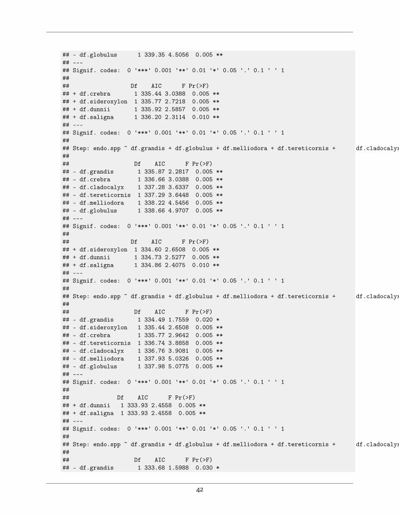
## - df.globulus 1 339.35 4.5056 0.005 **## ---## Signif. codes: 0 '***' 0.001 '**' 0.01 '*' 0.05 '.' 0.1 ' ' 1#### Df AIC F Pr(>F)## + df.crebra 1 335.44 3.0388 0.005 **## + df.sideroxylon 1 335.77 2.7218 0.005 **## + df.dunnii 1 335.92 2.5857 0.005 **## + df.saligna 1 336.20 2.3114 0.010 **## ---## Signif. codes: 0 '***' 0.001 '**' 0.01 '*' 0.05 '.' 0.1 ' ' 1#### Step: endo.spp ~ df.grandis + df.globulus + df.melliodora + df.tereticornis + df.cladocalyx + df.crebra#### Df AIC F Pr(>F)## - df.grandis 1 335.87 2.2817 0.005 **## - df.crebra 1 336.66 3.0388 0.005 **## - df.cladocalyx 1 337.28 3.6337 0.005 **## - df.tereticornis 1 337.29 3.6448 0.005 **## - df.melliodora 1 338.22 4.5456 0.005 **## - df.globulus 1 338.66 4.9707 0.005 **## ---## Signif. codes: 0 '***' 0.001 '**' 0.01 '*' 0.05 '.' 0.1 ' ' 1#### Df AIC F Pr(>F)## + df.sideroxylon 1 334.60 2.6508 0.005 **## + df.dunnii 1 334.73 2.5277 0.005 **## + df.saligna 1 334.86 2.4075 0.010 **## ---## Signif. codes: 0 '***' 0.001 '**' 0.01 '*' 0.05 '.' 0.1 ' ' 1#### Step: endo.spp ~ df.grandis + df.globulus + df.melliodora + df.tereticornis + df.cladocalyx + df.crebra + df.sideroxylon#### Df AIC F Pr(>F)## - df.grandis 1 334.49 1.7559 0.020 *## - df.sideroxylon 1 335.44 2.6508 0.005 **## - df.crebra 1 335.77 2.9642 0.005 **## - df.tereticornis 1 336.74 3.8858 0.005 **## - df.cladocalyx 1 336.76 3.9081 0.005 **## - df.melliodora 1 337.93 5.0326 0.005 **## - df.globulus 1 337.98 5.0775 0.005 **## ---## Signif. codes: 0 '***' 0.001 '**' 0.01 '*' 0.05 '.' 0.1 ' ' 1#### Df AIC F Pr(>F)## + df.dunnii 1 333.93 2.4558 0.005 **## + df.saligna 1 333.93 2.4558 0.005 **## ---## Signif. codes: 0 '***' 0.001 '**' 0.01 '*' 0.05 '.' 0.1 ' ' 1#### Step: endo.spp ~ df.grandis + df.globulus + df.melliodora + df.tereticornis + df.cladocalyx + df.crebra + df.sideroxylon + df.dunnii#### Df AIC F Pr(>F)## - df.grandis 1 333.68 1.5988 0.030 *
42
## - df.dunnii 1 334.60 2.4558 0.005 **## - df.sideroxylon 1 334.73 2.5774 0.005 **## - df.crebra 1 334.88 2.7219 0.005 **## - df.cladocalyx 1 335.30 3.1175 0.005 **## - df.tereticornis 1 335.82 3.6068 0.005 **## - df.globulus 1 336.17 3.9327 0.005 **## - df.melliodora 1 336.19 3.9490 0.005 **## ---## Signif. codes: 0 '***' 0.001 '**' 0.01 '*' 0.05 '.' 0.1 ' ' 1#### Df AIC F Pr(>F)## + df.saligna 0 333.93
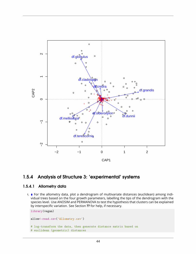
# look at ordistep resultstep.env$anova # presents results in an ANOVA-like table
## Df AIC F Pr(>F)## + df.grandis 1 342.88 3.9200 0.005 **## + df.globulus 1 341.06 3.7749 0.005 **## + df.melliodora 1 339.61 3.3666 0.005 **## + df.tereticornis 1 338.16 3.3325 0.005 **## + df.cladocalyx 1 336.66 3.3455 0.005 **## + df.crebra 1 335.44 3.0388 0.005 **## + df.sideroxylon 1 334.60 2.6508 0.005 **## + df.dunnii 1 333.93 2.4558 0.005 **## ---## Signif. codes: 0 '***' 0.001 '**' 0.01 '*' 0.05 '.' 0.1 ' ' 1
plot(step.env)
43
−2 −1 0 1 2
−2
−1
01
2
CAP1
CA
P2
+++++++++ +++++
++ + +++++++++++
+
+++++++
+
+++++++
++
++++++++++
++++++++++++++++++++ +++++
+++++++++++++++++++++++++++++++++++++++++++++++++++++++ +++
+
++ ++
++++++++++
+++++++
+
++++
+ +++++++++++++++++++++++ +
++++++++++ +++
+
+++++++++++++++++++++++++++++ ++++++
+++++
+
++++++++++++
+
+
+
+++++++++++++
++
+
+ +
+
++++++++++++++
+
+++++++++++++++++++++++
+++++++++++++++++++
+++++
+
++++++
+
+
+++++++
+++
+++++++++ ++++ + +
++++++++++++++++++++++++++++++++++++++++++++++++++++++++++++++++++++++++++++++++++ ++ +
+++++++++++++++++++++
+
+++++++++++++++++++++++ ++++++++ +++++++
++++ +++++
++++++++++++++++++++
+++++++++++++++++++++ ++++ ++
++
+
++
++
++++++++
+
++++++++++
+++++++++++++++++++++++++++++++++++++++ +
+
++++++++++++++++++++ ++++++++++++++ ++ +++++++++++++++
++++
++++++++++++++
+
++ +++++++++
+
++++ +++++
+++++++++++++++++++++
+
++
+++++
++++++++
+
++
+
+++++++++++
+
+++++++++++++++++++++++++++++++++++++++++++++++++++++++++++++++++
+
++++++++++++++++++++
df.grandis
df.globulus
df.melliodora
df.tereticornis
df.cladocalyx
df.crebra
df.sideroxylondf.dunnii
1.5.4 Analysis of Structure 3: ’experimental’ systems
1.5.4.1 Allometry data
1. ⧫ For the allometry data, plot a dendrogram of multivariate distances (euclidean) among indi-vidual trees based on the four growth parameters, labelling the tips of the dendrogram with thespecies level. Use ANOSIM and PERMANOVA to test the hypothesis that clusters can be explainedby interspecific variation. See Section ?? for help, if necessary.library(vegan)
allom<-read.csv('Allometry.csv')
# log-transform the data, then generate distance matrix based on# euclidean (geometric) distances
44

allom.dist <- vegdist(decostand(allom[,2:5],'log'),method='euclidean')
## Warning: non-integer data: divided by smallest positive value
# use hierarchical clustering to determine different levels of similarity among individualsallom.clust<-hclust(allom.dist)
# If the plotting window is too small, open one like this: windows()# (Or click 'Zoom')
# plot the hierarchical clustering result, specifying species with# the 'labels' argument.plot(allom.clust,labels=allom[,1])
PS
ME
PIM
OP
SM
EP
IMO PS
ME
PIP
OP
IPO
PIM
OP
SM
EP
IPO
PIP
O PS
ME
PIP
OP
IPO
PIP
OP
IPO
PIP
OP
IPO
PIM
OP
SM
EP
SM
EP
SM
EP
IMO
PS
ME
PIM
OP
IPO
PIP
OP
IPO
PS
ME
PIP
OP
IMO
PIM
OP
SM
EP
SM
EP
SM
EP
IMO
PIP
OP
IMO
PIM
OP
SM
EP
IMO
PIM
OP
IMO
PIM
OP
SM
EP
SM
EP
SM
EP
SM
EP
IMO
PIP
OP
IPO
PS
ME
PS
ME
PIM
OP
IPO
PIM
OP
IMO
PIP
OP
IPO
PIP
OP
SM
EP
SM
EP
IPO
02
46
810
12
Cluster Dendrogram
hclust (*, "complete")allom.dist
Hei
ght
# estimate the significance of tree species as a predictor of multivariate growth response# using ANOSIMallom.ano<-anosim(allom.dist,allom[,1])
45
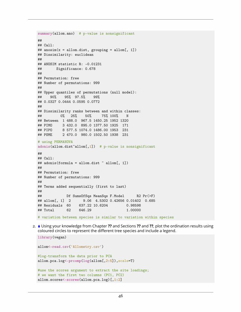
summary(allom.ano) # p-value is nonsignificant
#### Call:## anosim(x = allom.dist, grouping = allom[, 1])## Dissimilarity: euclidean#### ANOSIM statistic R: -0.01231## Significance: 0.678#### Permutation: free## Number of permutations: 999#### Upper quantiles of permutations (null model):## 90% 95% 97.5% 99%## 0.0327 0.0444 0.0595 0.0772#### Dissimilarity ranks between and within classes:## 0% 25% 50% 75% 100% N## Between 1 488.0 967.5 1450.25 1952 1320## PIMO 3 432.0 895.0 1377.50 1925 171## PIPO 8 577.5 1074.0 1486.00 1953 231## PSME 2 470.0 980.0 1502.50 1938 231
# using PERMANOVAadonis(allom.dist~allom[,1]) # p-value is nonsignificant
#### Call:## adonis(formula = allom.dist ~ allom[, 1])#### Permutation: free## Number of permutations: 999#### Terms added sequentially (first to last)#### Df SumsOfSqs MeanSqs F.Model R2 Pr(>F)## allom[, 1] 2 9.06 4.5302 0.42656 0.01402 0.685## Residuals 60 637.22 10.6204 0.98598## Total 62 646.29 1.00000
# variation between species is similar to variation within species
2. ⧫ Using your knowledge from Chapter ?? and Sections ?? and ??, plot the ordination results usingcoloured circles to represent the different tree species and include a legend.library(vegan)
allom<-read.csv('Allometry.csv')
#log-transform the data prior to PCAallom.pca.log<-prcomp(log(allom[,2:5]),scale=T)
#use the scores argument to extract the site loadings;# we want the first two columns (PC1, PC2)allom.scores<-scores(allom.pca.log)[,1:2]
46
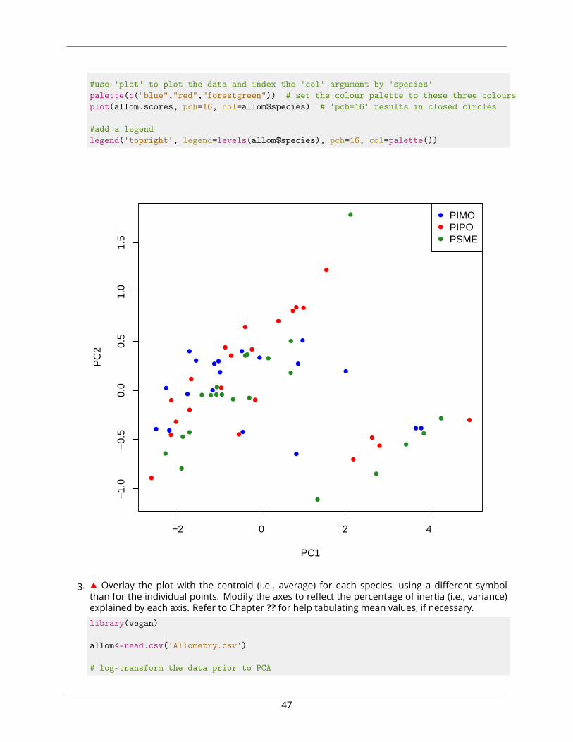
#use 'plot' to plot the data and index the 'col' argument by 'species'palette(c("blue","red","forestgreen")) # set the colour palette to these three coloursplot(allom.scores, pch=16, col=allom$species) # 'pch=16' results in closed circles
#add a legendlegend('topright', legend=levels(allom$species), pch=16, col=palette())
−2 0 2 4
−1.
0−
0.5
0.0
0.5
1.0
1.5
PC1
PC
2
PIMOPIPOPSME
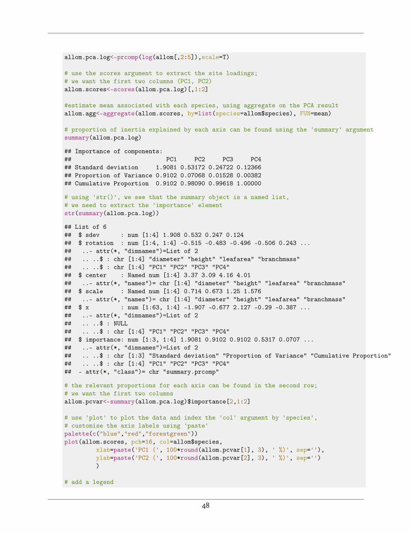
3. ▲ Overlay the plot with the centroid (i.e., average) for each species, using a different symbolthan for the individual points. Modify the axes to reflect the percentage of inertia (i.e., variance)explained by each axis. Refer to Chapter ?? for help tabulating mean values, if necessary.library(vegan)
allom<-read.csv('Allometry.csv')
# log-transform the data prior to PCA
47
allom.pca.log<-prcomp(log(allom[,2:5]),scale=T)
# use the scores argument to extract the site loadings;# we want the first two columns (PC1, PC2)allom.scores<-scores(allom.pca.log)[,1:2]
#estimate mean associated with each species, using aggregate on the PCA resultallom.agg<-aggregate(allom.scores, by=list(species=allom$species), FUN=mean)
# proportion of inertia explained by each axis can be found using the 'summary' argumentsummary(allom.pca.log)
## Importance of components:## PC1 PC2 PC3 PC4## Standard deviation 1.9081 0.53172 0.24722 0.12366## Proportion of Variance 0.9102 0.07068 0.01528 0.00382## Cumulative Proportion 0.9102 0.98090 0.99618 1.00000
# using 'str()', we see that the summary object is a named list,# we need to extract the 'importance' elementstr(summary(allom.pca.log))
## List of 6## $ sdev : num [1:4] 1.908 0.532 0.247 0.124## $ rotation : num [1:4, 1:4] -0.515 -0.483 -0.496 -0.506 0.243 ...## ..- attr(*, "dimnames")=List of 2## .. ..$ : chr [1:4] "diameter" "height" "leafarea" "branchmass"## .. ..$ : chr [1:4] "PC1" "PC2" "PC3" "PC4"## $ center : Named num [1:4] 3.37 3.09 4.16 4.01## ..- attr(*, "names")= chr [1:4] "diameter" "height" "leafarea" "branchmass"## $ scale : Named num [1:4] 0.714 0.673 1.25 1.576## ..- attr(*, "names")= chr [1:4] "diameter" "height" "leafarea" "branchmass"## $ x : num [1:63, 1:4] -1.907 -0.677 2.127 -0.29 -0.387 ...## ..- attr(*, "dimnames")=List of 2## .. ..$ : NULL## .. ..$ : chr [1:4] "PC1" "PC2" "PC3" "PC4"## $ importance: num [1:3, 1:4] 1.9081 0.9102 0.9102 0.5317 0.0707 ...## ..- attr(*, "dimnames")=List of 2## .. ..$ : chr [1:3] "Standard deviation" "Proportion of Variance" "Cumulative Proportion"## .. ..$ : chr [1:4] "PC1" "PC2" "PC3" "PC4"## - attr(*, "class")= chr "summary.prcomp"
# the relevant proportions for each axis can be found in the second row;# we want the first two columnsallom.pcvar<-summary(allom.pca.log)$importance[2,1:2]
# use 'plot' to plot the data and index the 'col' argument by 'species',# customise the axis labels using 'paste'palette(c("blue","red","forestgreen"))plot(allom.scores, pch=16, col=allom$species,
xlab=paste('PC1 (', 100*round(allom.pcvar[1], 3), ' %)', sep=''),ylab=paste('PC2 (', 100*round(allom.pcvar[2], 3), ' %)', sep=''))
# add a legend
48
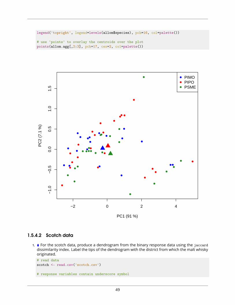
legend('topright', legend=levels(allom$species), pch=16, col=palette())
# use 'points' to overlay the centroids over the plotpoints(allom.agg[,2:3], pch=17, cex=2, col=palette())
−2 0 2 4
−1.
0−
0.5
0.0
0.5
1.0
1.5
PC1 (91 %)
PC
2 (7
.1 %
)
PIMOPIPOPSME
1.5.4.2 Scotch data
1. ⧫ For the scotch data, produce a dendrogram from the binary response data using the jaccarddissimilarity index. Label the tips of the dendrogram with the district from which the malt whiskyoriginated.# read datascotch <- read.csv('scotch.csv')
# response variables contain underscore symbol
49
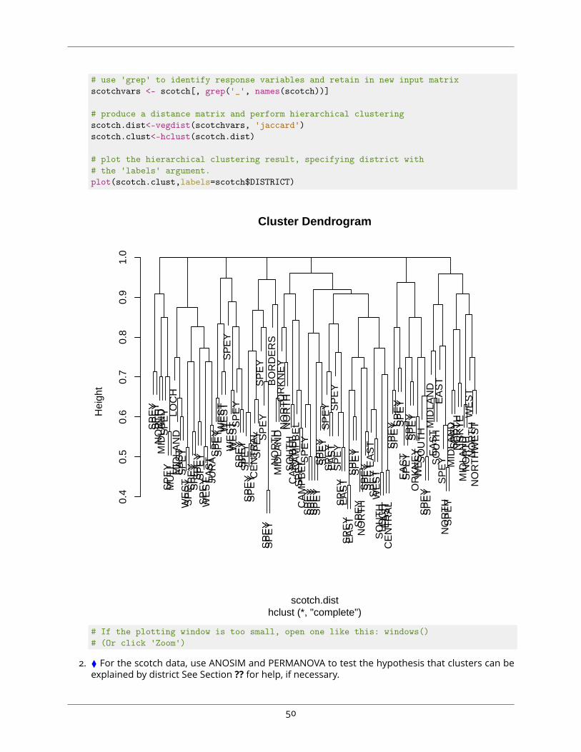
# use 'grep' to identify response variables and retain in new input matrixscotchvars <- scotch[, grep('_', names(scotch))]
# produce a distance matrix and perform hierarchical clusteringscotch.dist<-vegdist(scotchvars, 'jaccard')scotch.clust<-hclust(scotch.dist)
# plot the hierarchical clustering result, specifying district with# the 'labels' argument.plot(scotch.clust,labels=scotch$DISTRICT)
SP
EY
SP
EY
NO
RT
HM
IDLA
ND
SP
EY
SP
EY
MU
LLLO
CH
MID
LAN
DE
AS
TS
PE
YW
ES
TS
PE
Y SP
EY
SP
EY
SP
EY
SP
EY
SP
EY
WE
ST E
AS
TJU
RA
SP
EY
SP
EY W
ES
TW
ES
TS
PE
YW
ES
TW
ES
T SP
EY
SP
EY
SP
EY
SP
EY
SP
EY
SP
EY C
EN
TR
AL
SP
EY
SP
EY
SP
EY
SP
EY
SP
EY
BO
RD
ER
SN
OR
TH
MID
LAN
DO
RK
NE
YN
OR
TH
NO
RT
HS
OU
TH
CA
MP
BE
LC
AM
PB
EL
SP
EY
CA
MP
BE
L SP
EY
SP
EY
SP
EY
SP
EY
SP
EY
SP
EY
SP
EY
SP
EY
SP
EY
EA
ST
SP
EY
SP
EY
SP
EY
EA
ST
SP
EY
EA
ST
SP
EY
SP
EY
SP
EY
NO
RT
HS
PE
YS
PE
Y EA
ST
SP
EY
WE
ST
SO
UT
HLO
CH
EA
ST
CE
NT
RA
LS
PE
YS
PE
Y SP
EY
SP
EY
EA
ST
SP
EY
SP
EY
SP
EY
OR
KN
EY
WE
ST
SO
UT
HS
PE
YS
PE
YM
IDLA
ND
EA
ST
SO
UT
HE
AS
TS
PE
YN
OR
TH
SP
EY
MID
LAN
DS
PE
YN
OR
TH
SK
YE
MID
LAN
DN
OR
TH
WE
ST
NO
RT
HN
OR
TH
WE
ST
0.4
0.5
0.6
0.7
0.8
0.9
1.0
Cluster Dendrogram
hclust (*, "complete")scotch.dist
Hei
ght
# If the plotting window is too small, open one like this: windows()# (Or click 'Zoom')
2. ⧫ For the scotch data, use ANOSIM and PERMANOVA to test the hypothesis that clusters can beexplained by district See Section ?? for help, if necessary.
50
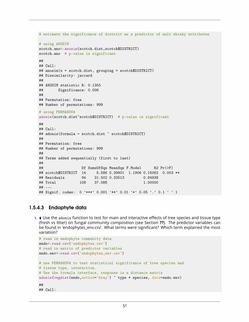
# estimate the significance of district as a predictor of malt whisky attributes
# using ANOSIMscotch.ano<-anosim(scotch.dist,scotch$DISTRICT)scotch.ano # p-value is significant
#### Call:## anosim(x = scotch.dist, grouping = scotch$DISTRICT)## Dissimilarity: jaccard#### ANOSIM statistic R: 0.1355## Significance: 0.006#### Permutation: free## Number of permutations: 999
# using PERMANOVAadonis(scotch.dist~scotch$DISTRICT) # p-value is significant
#### Call:## adonis(formula = scotch.dist ~ scotch$DISTRICT)#### Permutation: free## Number of permutations: 999#### Terms added sequentially (first to last)#### Df SumsOfSqs MeanSqs F.Model R2 Pr(>F)## scotch$DISTRICT 14 5.586 0.39901 1.1906 0.15062 0.003 **## Residuals 94 31.502 0.33513 0.84938## Total 108 37.088 1.00000## ---## Signif. codes: 0 '***' 0.001 '**' 0.01 '*' 0.05 '.' 0.1 ' ' 1
1.5.4.3 Endophyte data
1. ⧫ Use the adonis function to test for main and interactive effects of tree species and tissue type(fresh vs litter) on fungal community composition (see Section ??). The predictor variables canbe found in ‘endophytes_env.csv’. What terms were significant? Which term explained the mostvariation?# read in endophyte community dataendo<-read.csv('endophytes.csv')# read in matrix of predictor variablesendo.env<-read.csv('endophytes_env.csv')
# use PERMANOVA to test statistical significance of tree species and# tissue type, interaction.# Use the formula interface, response is a distance matrixadonis(vegdist(endo,method='bray') ~ type * species, data=endo.env)
#### Call:
51

## adonis(formula = vegdist(endo, method = "bray") ~ type * species, data = endo.env)#### Permutation: free## Number of permutations: 999#### Terms added sequentially (first to last)#### Df SumsOfSqs MeanSqs F.Model R2 Pr(>F)## type 1 3.498 3.4977 18.9119 0.10707 0.001 ***## species 8 7.885 0.9856 5.3291 0.24137 0.001 ***## type:species 8 6.488 0.8110 4.3852 0.19862 0.001 ***## Residuals 80 14.796 0.1849 0.45293## Total 97 32.666 1.00000## ---## Signif. codes: 0 '***' 0.001 '**' 0.01 '*' 0.05 '.' 0.1 ' ' 1
# all terms were significant, species had the largest R2
2. ▲ Plot the PCoA results and use different symbols and colours to reflect the identities of treespecies and tissue types. Add a legend to the plot. Use information from Chapter ?? and Sec-tions ?? and ?? for help, if necessary. Hint: automatic functions for generating vectors of colours,such as rainbow, can lead to very similar colours with so many treatment levels. Check out therandomcoloR package for alternative approaches.# read in endophyte community dataendo<-read.csv('endophytes.csv')# read in matrix of predictor variablesendo.env<-read.csv('endophytes_env.csv')
# perform PCoA, input is a distance matrixendo.pcoa<-wcmdscale(vegdist(endo,method='bray'))
# set up palettelibrary(randomcoloR)palette(randomColor(length(levels(endo.env$species))))
# plot PCoA results using scores() to extract the site loadings# eight colours indexed by species, two symbols indexed by tissue typeplot(scores(endo.pcoa,display='sites'),col=endo.env$species,
pch=c(1,16)[endo.env$type])# add a legend indicating tissue typelegend('bottomleft',levels(endo.env$type),pch=c(1,16))# add a legend indicating tree specieslegend('bottomright',levels(endo.env$species),col=palette(),pch=16,cex=0.75)
52
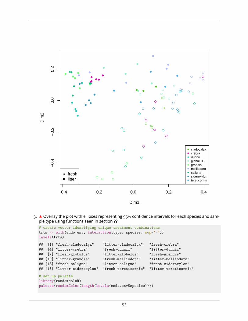
−0.4 −0.2 0.0 0.2 0.4
−0.
4−
0.2
0.0
0.2
Dim1
Dim
2
freshlitter
cladocalyxcrebradunniiglobulusgrandismelliodorasalignasideroxylontereticornis
3. ▲ Overlay the plot with ellipses representing 95% confidence intervals for each species and sam-ple type using functions seen in section ??.# create vector identifying unique treatment combinationstrts <- with(endo.env, interaction(type, species, sep='-'))levels(trts)
## [1] "fresh-cladocalyx" "litter-cladocalyx" "fresh-crebra"## [4] "litter-crebra" "fresh-dunnii" "litter-dunnii"## [7] "fresh-globulus" "litter-globulus" "fresh-grandis"## [10] "litter-grandis" "fresh-melliodora" "litter-melliodora"## [13] "fresh-saligna" "litter-saligna" "fresh-sideroxylon"## [16] "litter-sideroxylon" "fresh-tereticornis" "litter-tereticornis"
# set up palettelibrary(randomcoloR)palette(randomColor(length(levels(endo.env$species))))
53
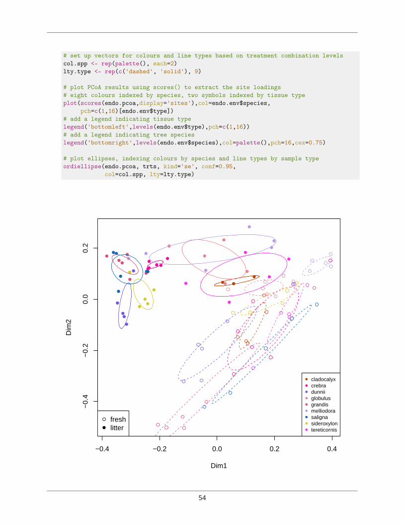
# set up vectors for colours and line types based on treatment combination levelscol.spp <- rep(palette(), each=2)lty.type <- rep(c('dashed', 'solid'), 9)
# plot PCoA results using scores() to extract the site loadings# eight colours indexed by species, two symbols indexed by tissue typeplot(scores(endo.pcoa,display='sites'),col=endo.env$species,
pch=c(1,16)[endo.env$type])# add a legend indicating tissue typelegend('bottomleft',levels(endo.env$type),pch=c(1,16))# add a legend indicating tree specieslegend('bottomright',levels(endo.env$species),col=palette(),pch=16,cex=0.75)
# plot ellipses, indexing colours by species and line types by sample typeordiellipse(endo.pcoa, trts, kind='se', conf=0.95,
col=col.spp, lty=lty.type)
−0.4 −0.2 0.0 0.2 0.4
−0.
4−
0.2
0.0
0.2
Dim1
Dim
2
freshlitter
cladocalyxcrebradunniiglobulusgrandismelliodorasalignasideroxylontereticornis
54
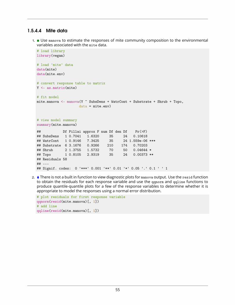
1.5.4.4 Mite data
1. ∎ Use manova to estimate the responses of mite community composition to the environmentalvariables associated with the mite data.# load librarylibrary(vegan)
# load 'mite' datadata(mite)data(mite.env)
# convert response table to matrixY <- as.matrix(mite)
# fit modelmite.manova <- manova(Y ~ SubsDens + WatrCont + Substrate + Shrub + Topo,
data = mite.env)
# view model summarysummary(mite.manova)
## Df Pillai approx F num Df den Df Pr(>F)## SubsDens 1 0.7041 1.6320 35 24 0.10618## WatrCont 1 0.9146 7.3425 35 24 1.559e-06 ***## Substrate 6 3.1676 0.9266 210 174 0.70203## Shrub 2 1.3755 1.5732 70 50 0.04644 *## Topo 1 0.8105 2.9319 35 24 0.00373 **## Residuals 58## ---## Signif. codes: 0 '***' 0.001 '**' 0.01 '*' 0.05 '.' 0.1 ' ' 1
2. ⧫ There is not a built in function to view diagnostic plots for manova output. Use the resid functionto obtain the residuals for each response variable and use the qqnorm and qqline functions toproduce quantile-quantile plots for a few of the response variables to determine whether it isappropriate to model the responses using a normal error distribution.# plot residuals for first response variableqqnorm(resid(mite.manova)[, 1])# add lineqqline(resid(mite.manova)[, 1])
55
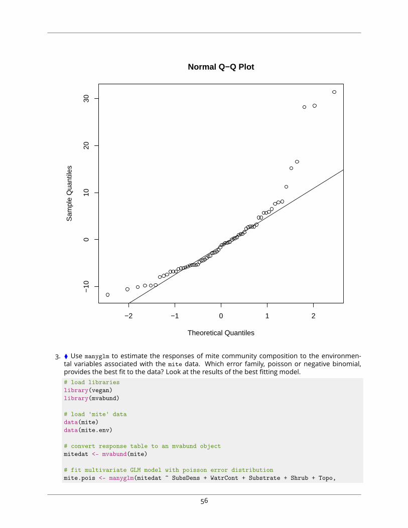
−2 −1 0 1 2
−10
010
2030
Normal Q−Q Plot
Theoretical Quantiles
Sam
ple
Qua
ntile
s
3. ⧫ Use manyglm to estimate the responses of mite community composition to the environmen-tal variables associated with the mite data. Which error family, poisson or negative binomial,provides the best fit to the data? Look at the results of the best fitting model.# load librarieslibrary(vegan)library(mvabund)
# load 'mite' datadata(mite)data(mite.env)
# convert response table to an mvabund objectmitedat <- mvabund(mite)
# fit multivariate GLM model with poisson error distributionmite.pois <- manyglm(mitedat ~ SubsDens + WatrCont + Substrate + Shrub + Topo,
56

data = mite.env, family='poisson')
# fit multivariate GLM model with negative binomial error distributionmite.nbin <- manyglm(mitedat ~ SubsDens + WatrCont + Substrate + Shrub + Topo,
data = mite.env, family='negative.binomial')
# view model diagnosticsplot(mite.pois)
−6 −4 −2 0 2 4 6
−10
−5
05
10
Linear predictor value
Dun
n−S
myt
h R
esid
uals
manyglm(mitedat ~ SubsDens + WatrCont + Substrate + Shrub + Topo ...)
Residuals vs Fitted
plot(mite.nbin)
57
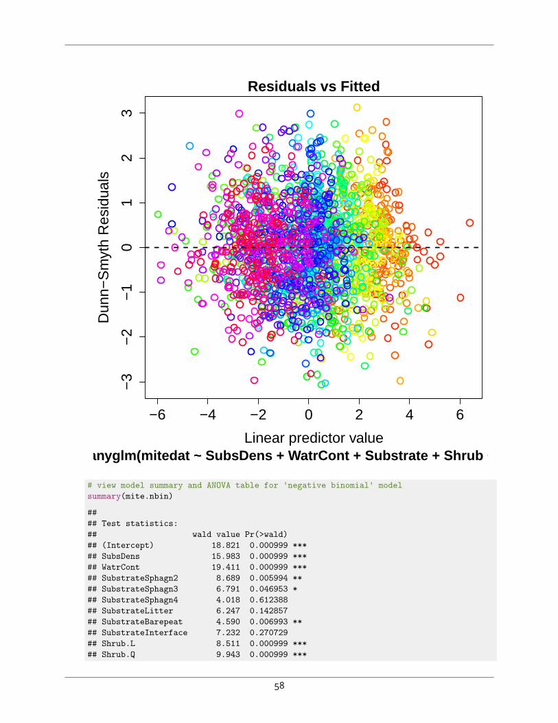
−6 −4 −2 0 2 4 6
−3
−2
−1
01
23
Linear predictor value
Dun
n−S
myt
h R
esid
uals
manyglm(mitedat ~ SubsDens + WatrCont + Substrate + Shrub + Topo ...)
Residuals vs Fitted
# view model summary and ANOVA table for 'negative binomial' modelsummary(mite.nbin)
#### Test statistics:## wald value Pr(>wald)## (Intercept) 18.821 0.000999 ***## SubsDens 15.983 0.000999 ***## WatrCont 19.411 0.000999 ***## SubstrateSphagn2 8.689 0.005994 **## SubstrateSphagn3 6.791 0.046953 *## SubstrateSphagn4 4.018 0.612388## SubstrateLitter 6.247 0.142857## SubstrateBarepeat 4.590 0.006993 **## SubstrateInterface 7.232 0.270729## Shrub.L 8.511 0.000999 ***## Shrub.Q 9.943 0.000999 ***
58

## TopoHummock 12.950 0.000999 ***## ---## Signif. codes: 0 '***' 0.001 '**' 0.01 '*' 0.05 '.' 0.1 ' ' 1#### Test statistic: 36.88, p-value: 0.000999## Arguments:## Test statistics calculated assuming response assumed to be uncorrelated## P-value calculated using 1000 resampling iterations via pit.trap resampling (to account for correlation in testing).
anova(mite.nbin)
## Time elapsed: 0 hr 4 min 9 sec## Analysis of Deviance Table#### Model: manyglm(formula = mitedat ~ SubsDens + WatrCont + Substrate +## Model: Shrub + Topo, family = "negative.binomial", data = mite.env)#### Multivariate test:## Res.Df Df.diff Dev Pr(>Dev)## (Intercept) 69## SubsDens 68 1 73.5 0.014 *## WatrCont 67 1 600.3 0.001 ***## Substrate 61 6 306.9 0.025 *## Shrub 59 2 247.7 0.001 ***## Topo 58 1 146.2 0.002 **## ---## Signif. codes: 0 '***' 0.001 '**' 0.01 '*' 0.05 '.' 0.1 ' ' 1## Arguments:## Test statistics calculated assuming uncorrelated response (for faster computation)## P-value calculated using 999 resampling iterations via PIT-trap resampling (to account for correlation in testing).
59


![[ Seco ]marod/web-data/score-samples/seco-sample.pdfRub stones Œ Œ ∏ Ö f f f f 5 ƒ ƒ ƒf ƒ f ƒ ƒ ƒ ƒ ƒ ƒ ® ® ® ® ® ® ‰ ≈ ≈ ‰ ‰ π π π Whip bow Œ Œ](https://static.fdocuments.us/doc/165x107/610b6a6961269e25150c7bae/-seco-marodweb-datascore-samplesseco-samplepdf-rub-stones-a-f.jpg)