Apr. 2007Computer Arithmetic, Number RepresentationSlide 1 Part I Number Representation.

Apr. 2007 Computer Arithmetic, Number Representation Slide 1

Part INumber Representation

Number Representation

Numbers and Arithmetic Representing Signed Numbers Redundant Number Systems Residue Number Systems

Addition / Subtraction

Basic Addition and Counting Carry-Lookahead Adders Variations in Fast Adders Multioperand Addition

Multiplication

Basic Multiplication Schemes High-Radix Multipliers Tree and Array Multipliers Variations in Multipliers

Division

Basic Division Schemes High-Radix Dividers Variations in Dividers Division by Convergence

Real Arithmetic

Floating-Point Reperesentations Floating-Point Operations Errors and Error Control Precise and Certifiable Arithmetic

Function Evaluation

Square-Rooting Methods The CORDIC Algorithms Variations in Function Evaluation Arithmetic by Table Lookup

Implementation Topics

High-Throughput Arithmetic Low-Power Arithmetic Fault-Tolerant Arithmetic Past, Present, and Future

Parts Chapters

I.

II.

III.

IV.

V.

VI.

VII.

1. 2. 3. 4.

5. 6. 7. 8.

9. 10. 11. 12.

25. 26. 27. 28.

21. 22. 23. 24.

17. 18. 19. 20.

13. 14. 15. 16.

Ele

me

ntar

y O

pera

tions


About This Presentation

This presentation is intended to support the use of the textbook Computer Arithmetic: Algorithms and Hardware Designs (Oxford University Press, 2000, ISBN 0-19-512583-5). It is updated regularly by the author as part of his teaching of the graduate course ECE 252B, Computer Arithmetic, at the University of California, Santa Barbara. Instructors can use these slides freely in classroom teaching and for other educational purposes. Unauthorized uses are strictly prohibited. © Behrooz Parhami

Edition Released Revised Revised Revised Revised

First Jan. 2000 Sep. 2001 Sep. 2003 Sep. 2005 Apr. 2007


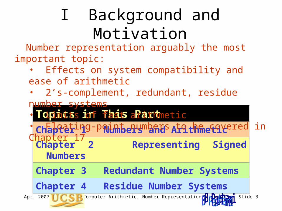
I Background and Motivation

Topics in This PartChapter 1 Numbers and Arithmetic

Chapter 2 Representing Signed Numbers

Chapter 3 Redundant Number Systems

Chapter 4 Residue Number Systems

Number representation arguably the most important topic:• Effects on system compatibility and ease of arithmetic• 2’s-complement, redundant, residue number systems• Limits of fast arithmetic• Floating-point numbers to be covered in Chapter 17


“This can’t be right . . . It goes into the red!”


1 Numbers and Arithmetic

Chapter Goals

Define scope and provide motivationSet the framework for the rest of the bookReview positional fixed-point numbers

Chapter Highlights

What goes on inside your calculator?Ways of encoding numbers in k bitsRadices and digit sets: conventional, exoticConversion from one system to another


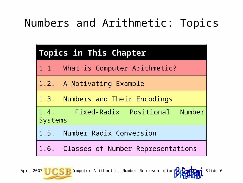
Numbers and Arithmetic: Topics

Topics in This Chapter

1.1. What is Computer Arithmetic?

1.2. A Motivating Example

1.3. Numbers and Their Encodings

1.4. Fixed-Radix Positional Number Systems

1.5. Number Radix Conversion

1.6. Classes of Number Representations


1.1 What is Computer Arithmetic?

Pentium Division Bug (1994-95): Pentium’s radix-4 SRT algorithm occasionally gave incorrect quotient First noted in 1994 by T. Nicely who computed sums of reciprocals of twin primes:

1/5 + 1/7 + 1/11 + 1/13 + . . . + 1/p + 1/(p + 2) + . . .

Worst-case example of division error in Pentium:


Top Ten Intel Slogans for the Pentium

Humor, circa 1995

• 9.999 997 325 It’s a FLAW, dammit, not a bug• 8.999 916 336 It’s close enough, we say so• 7.999 941 461 Nearly 300 correct opcodes• 6.999 983 153 You don’t need to know what’s inside• 5.999 983 513 Redefining the PC –– and math as well• 4.999 999 902 We fixed it, really• 3.999 824 591 Division considered harmful• 2.999 152 361 Why do you think it’s called “floating” point?• 1.999 910 351 We’re looking for a few good flaws• 0.999 999 999 The errata inside


Aspects of, and Topics in, Computer Arithmetic

Fig. 1.1 The scope of computer arithmetic.

Hardware (our focus in this book) Software––––––––––––––––––––––––––––––––––––––––––––––––– ––––––––––––––––––––––––––––––––––––

Design of efficient digital circuits for Numerical methods for solvingprimitive and other arithmetic operations systems of linear equations,such as +, –, , , , log, sin, cos partial differential equations, etc.

Issues: Algorithms Issues: AlgorithmsError analysis Error analysisSpeed/cost trade-offs Computational complexityHardware implementation ProgrammingTesting, verification Testing, verification

General-purpose Special-purpose–––––––––––––––––––––– –––––––––––––––––––––––

Flexible data paths Tailored toFast primitive applications like: operations like Digital filtering +, –, , , Image processingBenchmarking Radar tracking


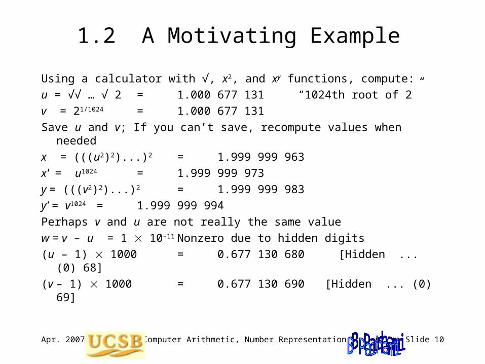
Using a calculator with √, x2, and xy functions, compute:

u = √√ … √ 2 = 1.000 677 131 “1024th root of 2”

v = 21/1024 = 1.000 677 131

Save u and v; If you can’t save, recompute values when needed

x = (((u2)2)...)2 = 1.999 999 963

x' = u1024 = 1.999 999 973

y = (((v2)2)...)2 = 1.999 999 983

y' = v1024 = 1.999 999 994

Perhaps v and u are not really the same value

w = v – u = 1 10–11 Nonzero due to hidden digits

(u – 1) 1000 = 0.677 130 680 [Hidden ... (0) 68]

(v – 1) 1000 = 0.677 130 690 [Hidden ... (0) 69]

1.2 A Motivating Example


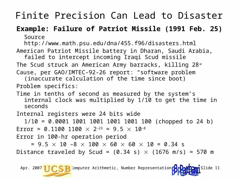
Finite Precision Can Lead to Disaster

Example: Failure of Patriot Missile (1991 Feb. 25)Source http://www.math.psu.edu/dna/455.f96/disasters.html

American Patriot Missile battery in Dharan, Saudi Arabia, failed to intercept incoming Iraqi Scud missile

The Scud struck an American Army barracks, killing 28 Cause, per GAO/IMTEC-92-26 report: “software problem” (inaccurate

calculation of the time since boot)Problem specifics: Time in tenths of second as measured by the system’s internal clock

was multiplied by 1/10 to get the time in seconds Internal registers were 24 bits wide

1/10 = 0.0001 1001 1001 1001 1001 100 (chopped to 24 b)Error ≈ 0.1100 1100 2–23 ≈ 9.5 10–8 Error in 100-hr operation period

≈ 9.5 10 –8 100 60 60 10 = 0.34 sDistance traveled by Scud = (0.34 s) (1676 m/s) ≈ 570 m


Finite Range Can Lead to Disaster

Example: Explosion of Ariane Rocket (1996 June 4)Source http://www.math.psu.edu/dna/455.f96/disasters.html

Unmanned Ariane 5 rocket of the European Space Agency veered off its flight path, broke up, and exploded only 30 s after lift-off (altitude of 3700 m)

The $500 million rocket (with cargo) was on its first voyage after a decade of development costing $7 billion

Cause: “software error in the inertial reference system”Problem specifics: A 64 bit floating point number relating to the horizontal velocity of the

rocket was being converted to a 16 bit signed integerAn SRI* software exception arose during conversion because the

64-bit floating point number had a value greater than what could be represented by a 16-bit signed integer (max 32 767)

*SRI = Système de Référence Inertielle or Inertial Reference System


1.3 Numbers and Their Encodings

Some 4-bit number representation formats

Base-2logarithm

Exponent in{2, 1, 0, 1}

Significand in{0, 1, 2, 3}


Encoding Numbers in 4 Bits

Fig. 1.2 Some of the possible ways of assigning 16 distinct codes to represent numbers.

0 2 4 6 8 10 12 14 16 2 4 6 8 10 12 14 16

Unsigned integers

Signed-magnitude

3 + 1 fixed-point, xxx.x

Signed fraction, .xxx

2’s-compl. fraction, x.xxx

2 + 2 floating-point, s 2 e in [ 2, 1], s in [0, 3]

2 + 2 logarithmic (log = xx.xx)

Number format

log x

s e e


1.4 Fixed-Radix Positional Number Systems

( xk–1xk–2 . . . x1x0 . x–1x–2 . . . x–l )r = xi r i

One can generalize to:

Arbitrary radix (not necessarily integer, positive, constant)

Arbitrary digit set, usually {–, –+1, . . . , –1, } = [–, ]

Example 1.1. Balanced ternary number system:

Radix r = 3, digit set = [–1, 1]

Example 1.2. Negative-radix number systems:

Radix –r, r 2, digit set = [0, r – 1]

The special case with radix –2 and digit set [0, 1]

is known as the negabinary number system

1k

li


More Examples of Number Systems

Example 1.3. Digit set [–4, 5] for r = 10:

(3 –1 5)ten represents 295 = 300 – 10 + 5

Example 1.4. Digit set [–7, 7] for r = 10:

(3 –1 5)ten = (3 0 –5)ten = (1 –7 0 –5)ten

Example 1.7. Quater-imaginary number system:

radix r = 2j, digit set [0, 3]


1.5 Number Radix Conversion

Radix conversion, using arithmetic in the old radix r Convenient when converting from r = 10

u = w . v = ( xk–1xk–2 . . . x1x0 . x–1x–2 . . . x–l )r Old

= ( XK–1XK–2 . . . X1X0 . X–1X–2 . . . X–L )R New

Radix conversion, using arithmetic in the new radix R Convenient when converting to R = 10

Whole part Fractional part

Example: (31)eight = (25)ten 31 Oct. = 25 Dec. Halloween = Xmas


Radix Conversion: Old-Radix Arithmetic

Converting whole part w: (105)ten = (?)fiveRepeatedly divide by five Quotient Remainder

105 0 21 1 4 4 0

Therefore, (105)ten = (410)five

Converting fractional part v: (105.486)ten = (410.?)fiveRepeatedly multiply by five Whole Part Fraction

.486 2 .430 2 .150 0 .750 3 .750 3 .750

Therefore, (105.486)ten (410.22033)five


Radix Conversion: New-Radix Arithmetic

Converting whole part w: (22033)five = (?)ten

((((2 5) + 2) 5 + 0) 5 + 3) 5 + 3

|-----| : : : :

10 : : : :

|-----------| : : :

12 : : :

|---------------------| : :

60 : :

|-------------------------------| :

303 :

|-----------------------------------------|

1518

Converting fractional part v: (410.22033)five = (105.?)ten (0.22033)five 55 = (22033)five = (1518)ten

1518 / 55 = 1518 / 3125 = 0.48576Therefore, (410.22033)five = (105.48576)ten

Horner’s rule is also applicable: Proceed from right to left and use division instead of multiplication

Horner’srule or formula


Horner’s Rule for Fractions

Converting fractional part v: (0.22033)five = (?)ten

(((((3 / 5) + 3) / 5 + 0) / 5 + 2) / 5 + 2) / 5

|-----| : : : :

0.6 : : : :

|-----------| : : :

3.6 : : :

|---------------------| : :

0.72 : :

|-------------------------------| :

2.144 :

|-----------------------------------------|

2.4288

|-----------------------------------------------|

0.48576

Horner’srule or formula

Fig. 1.3 Horner’s rule used to convert (0.220 33)five to decimal.


1.6 Classes of Number RepresentationsIntegers (fixed-point), unsigned: Chapter 1

Integers (fixed-point), signed Signed-magnitude, biased, complement: Chapter 2 Signed-digit, including carry/borrow-save: Chapter 3 (but the key point of Chapter 3 is using redundancy for faster arithmetic, not how to represent signed values) Residue number system: Chapter 4 (again, the key to Chapter 4 is use of parallelism for faster arithmetic, not how to represent signed values)

Real numbers, floating-point: Chapter 17 Part V deals with real arithmetic

Real numbers, exact: Chapter 20 Continued-fraction, slash, . . .

For the most part you need:

The 2’s complement format Carry-save representation ANSI/IEEE FLP format

However, knowing the rest of the material (including RNS) provides you with more options when designing custom and special-purpose hardware systems


2 Representing Signed Numbers

Chapter Goals

Learn different encodings of the sign infoDiscuss implications for arithmetic design

Chapter Highlights

Using sign bit, biasing, complementationProperties of 2’s-complement numbersSigned vs unsigned arithmeticSigned numbers, positions, or digits


Representing Signed Numbers: Topics


2.1. Signed-Magnitude Representation

2.2. Biased Representations

2.3. Complement Representations

2.4. Two’s- and 1’s-Complement Numbers

2.5. Direct and Indirect Signed Arithmetic

2.6. Using Signed Positions or Signed Digits


2.1 Signed-Magnitude Representation

Fig. 2.1 Four-bit signed-magnitude number representation system for integers.

0000 0001 1111

0010 1110

0011 1101

0100 1100

1000

0101 1011

0110 1010

0111 1001

0 +1

+3

+4

+5

+6 +7

-7

-3

-5

-4

-0 -1

+2-

+ _

Bit pattern (representation)

Signed values (signed magnitude)

+2 -6

Increment Decrement

-


Signed-Magnitude Adder

Fig. 2.2 Adding signed-magnitude numbers using precomplementation and postcomplementation.

Adder cc

s

x ySign x Sign y

Sign

Sign s

Selective Complement


out in

Comp x

Control

Comp s

Add/Sub

Compl x

___ Add/Sub

Compl s

Selective complement



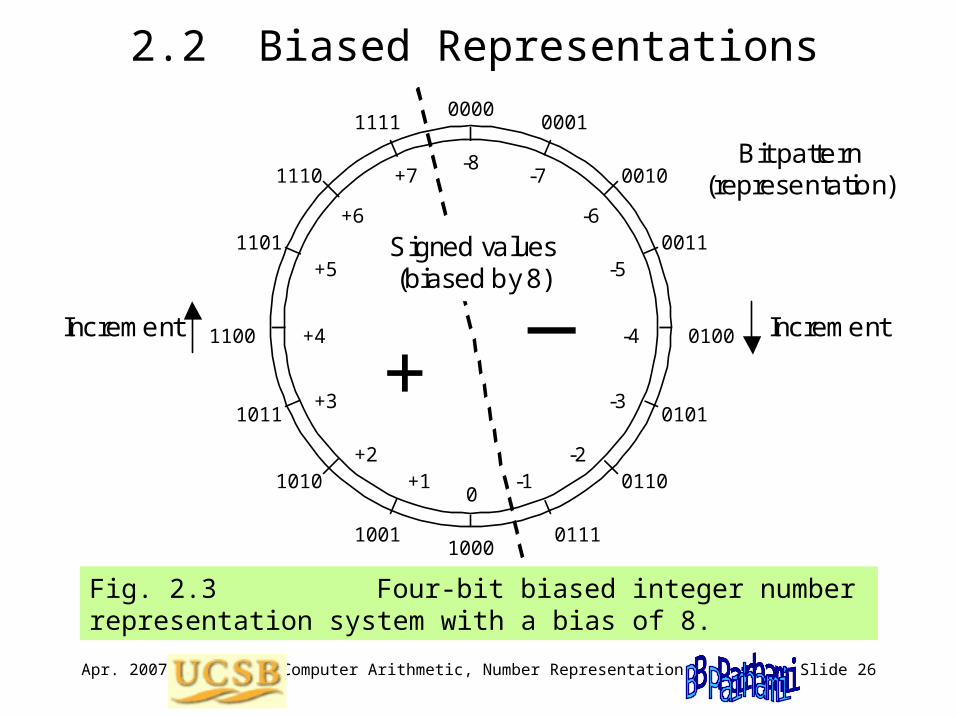
2.2 Biased Representations

Fig. 2.3 Four-bit biased integer number representation system with a bias of 8.

0000 0001 1111

0010 1110

0011 1101

0100 1100

1000

0101 1011

0110 1010

0111 1001

-8 -7

-5

-4

-3

-2 -1

+7

+3

+5

+4

0 +1

+2

+ _

Bit pattern (representation)

Signed values (biased by 8)

-6 +6

Increment Increment


Arithmetic with Biased Numbers

Addition/subtraction of biased numbersx + y + bias = (x + bias) + (y + bias) – biasx – y + bias = (x + bias) – (y + bias) + bias

A power-of-2 (or 2a – 1) bias simplifies addition/subtraction

Comparison of biased numbers:Compare like ordinary unsigned numbersfind true difference by ordinary subtraction

We seldom perform arbitrary arithmetic on biased numbersMain application: Exponent field of floating-point numbers


2.3 Complement Representations

Fig. 2.4 Complement representation of signed integers.

0 1

2

3

4

M - N

P

+0 +1

+3

+4

-1

+ _

Unsigned representations

Signed values

+2 -2

+ P - N

M - 1

M - 2

Increment Decrement


Arithmetic with Complement Representations

–––––––––––––––––––––––––––––––––––––––––––––––––––––––––––Desired Computation to be Correct result Overflowoperation performed mod M with no overflow condition–––––––––––––––––––––––––––––––––––––––––––––––––––––––––––(+x) + (+y) x + y x + y x + y > P

(+x) + (–y) x + (M – y) x – y if y x N/AM – (y – x) if y > x

(–x) + (+y) (M – x) + y y – x if x y N/AM – (x – y) if x > y

(–x) + (–y) (M – x) + (M – y) M – (x + y) x + y > N–––––––––––––––––––––––––––––––––––––––––––––––––––––––––––

Table 2.1 Addition in a complement number system with complementation constant M and range [–N, +P]


Example and Two Special Cases

Example -- complement system for fixed-point numbers:Complementation constant M = 12.000Fixed-point number range [–6.000, +5.999]Represent –3.258 as 12.000 – 3.258 = 8.742

Auxiliary operations for complement representationscomplementation or change of sign (computing M – x) computations of residues mod M

Thus, M must be selected to simplify these operations

Two choices allow just this for fixed-point radix-r arithmetic with k whole digits and l fractional digits

Radix complement M = rk

Digit complement M = rk – ulp (aka diminished radix compl)

ulp (unit in least position) stands for rl Allows us to forget about l, even for nonintegers


2.4 Two’s- and 1’s-Complement Numbers

Fig. 2.5 A 4-bit 2’s-complement number representation system for integers.

0000 0001 1111

0010 1110

0011 1101

0100 1100

1000

0101 1011

0110 1010

0111 1001

+0 +1

+3

+4

+5

+6 +7

-1

-5

-3

-4

-8 -7

-6

+ _


Signed values (2’s complement)

+2 -2

Two’s complement = radix complement system for r = 2

M = 2k

2k – x = [(2k – ulp) – x] + ulp = xcompl + ulp

Range of representable numbers in with k whole bits:

from –2k–1 to 2k–1 – ulp


One’s-Complement Number Representation

Fig. 2.6 A 4-bit 1’s-complement number representation system for integers.

One’s complement = digit complement (diminished radix complement) system for r = 2

M = 2k – ulp

(2k – ulp) – x = xcompl

Range of representable numbers in with k whole bits:

from –2k–1 + ulp to 2k–1 – ulp

0000 0001 1111

0010 1110

0011 1101

0100 1100

1000

0101 1011

0110 1010

0111 1001

+0 +1

+3

+4

+5

+6 +7

-0

-4

-2

-3

-7 -6

-5

+ _


Signed values (1’s complement)

+2 -1


Some Details for 2’s- and 1’s Complement

Range/precision extension for 2’s-complement numbers . . . xk–1 xk–1 xk–1 xk–1 xk–2 . . . x1 x0 . x–1 x–2 . . . x–l 0 0 0 . . .

Sign extension Sign LSD Extension bit

Range/precision extension for 1’s-complement numbers . . . xk–1 xk–1 xk–1 xk–1 xk–2 . . . x1 x0 . x–1 x–2 . . . x–l xk–1 xk–1 xk–1 . . .

Sign extension Sign LSD Extension bit

Mod-(2k – ulp) operation needed in 1’s-complement arithmetic is done via end-around carry

(x + y) – (2k – ulp) = (x – y – 2k) + ulp Connect cout to cin

Mod-2k operation needed in 2’s-complement arithmetic is trivial:Simply drop the carry-out (subtract 2k if result is 2k or greater)


Which Complement System Is Better?

–––––––––––––––––––––––––––––––––––––––––––––––––––––––––––Feature/Property Radix complement Digit complement–––––––––––––––––––––––––––––––––––––––––––––––––––––––––––Symmetry (P = N?) Possible for odd r Possible for even r

(radices of practicalinterest are even)

Unique zero? Yes No, there are two 0s

Complementation Complement all digits Complement all digitsand add ulp

Mod-M addition Drop the carry-out End-around carry–––––––––––––––––––––––––––––––––––––––––––––––––––––––––––

Table 2.2 Comparing radix- and digit-complement number representation systems


Why 2’s-Complement Is the Universal Choice

Fig. 2.7 Adder/subtractor architecture for 2’s-complement numbers.

Mux

Adder

0 1

x y

y or y _

s = x y

add/sub ___

c in

Controlled complementation

0 for addition, 1 for subtraction

c out

Can replace this mux with k XOR gates


Signed-Magnitude vs 2’s-Complement

Fig. 2.7

Mux

Adder

0 1

x y

y or y _

s = x y

add/sub ___

c in

Controlled complementation

0 for addition, 1 for subtraction

c out

Adder cc

s

x ySign x Sign y

Sign

Sign s



out in

Comp x

Control

Comp s

Add/Sub

Compl x

___ Add/Sub

Compl s



Fig. 2.2

Signed-magnitude adder/subtractor is significantly more complex than a simple adder

Two’s-complement adder/subtractor needs very little hardware other than a simple adder


2.5 Direct and Indirect Signed Arithmetic

Direct signed arithmetic is usually faster (not always)

Indirect signed arithmetic can be simpler (not always); allows sharing of signed/unsigned hardware when both operation types are needed

Fig. 2.8 Direct versus indirect operation on signed numbers.

x y

f

x y

f(x, y)

Sign logic

Unsigned operation

Sign removal

f(x, y)

Adjustment


2.6 Using Signed Positions or Signed Digits

A key property of 2’s-complement numbers that facilitates direct signed arithmetic:

Fig. 2.9 Interpreting a 2’s-complement number as having a negatively weighted most-significant digit.

x = (1 0 1 0 0 1 1 0)two’s-compl

–27 26 25 24 23 22 21 20

–128 + 32 + 4 + 2 = –90

Check: x = (1 0 1 0 0 1 1 0)two’s-compl

–x = (0 1 0 1 1 0 1 0)two

27 26 25 24 23 22 21 20

64 + 16 + 8 + 2 = 90


Associating a Sign with Each Digit

Fig. 2.10 Converting a standard radix-4 integer to a radix-4 integer with the nonstandard digit set [–1, 2].

3 1 2 0 2 3 Original digits in [0, 3]

–1 1 2 0 2 –1

1 0 0 0 0 1

Rewritten digits in [–1, 2]

Transfer digits in [0, 1]

1 –1 1 2 0 3 –1

1 –1 1 2 0 –1 –1

0 0 0 0 1 0

1 –1 1 2 1 –1 –1

Sum digits in [–1, 3]

Rewritten digits in [–1, 2]


Sum digits in [–1, 3]

Signed-digit representation: Digit set [, ] instead of [0, r – 1]

Example: Radix-4 representation with digit set [1, 2] rather than [0, 3]


Redundant Signed-Digit Representations

Fig. 2.11 Converting a standard radix-4 integer to a radix-4 integer with the nonstandard digit set [–2, 2].

Signed-digit representation: Digit set [, ], with = + + 1 – r > 0

Example: Radix-4 representation with digit set [2, 2]

3 1 2 0 2 3 Original digits in [0, 3]

–1 1 –2 0 –2 1

1 0 1 0 1 1

Interim digits in [–2, 1]


1 –1 2 –2 1 –1 –1 Sum digits in [–2, 2]

Here, the transfer does not propagate, so conversion is “carry-free”


3 Redundant Number Systems

Chapter Goals

Explore the advantages and drawbacks of using more than r digit values in radix r

Chapter Highlights

Redundancy eliminates long carry chainsRedundancy takes many forms: trade-offsConversions between redundant

and nonredundant representationsRedundancy used for end values too?


Redundant Number Systems: Topics


3.1. Coping with the Carry Problem

3.2. Redundancy in Computer Arithmetic

3.3. Digit Sets and Digit-Set Conversions

3.4. Generalized Signed-Digit Numbers

3.5. Carry-Free Addition Algorithms

3.6. Conversions and Support Functions


3.1 Coping with the Carry Problem

Ways of dealing with the carry propagation problem:

1. Limit propagation to within a small number of bits (Chapters 3-4)

2. Detect end of propagation; don’t wait for worst case (Chapter 5)

3. Speed up propagation via lookahead etc. (Chapters 6-7)

4. Ideal: Eliminate carry propagation altogether! (Chapter 3)

5 7 8 2 4 9

6 2 9 3 8 9 Operand digits in [0, 9] ––––––––––––––––––––––––––––––––––11 9 17 5 12 18 Position sums in [0, 18]

But how can we extend this beyond a single addition?

+


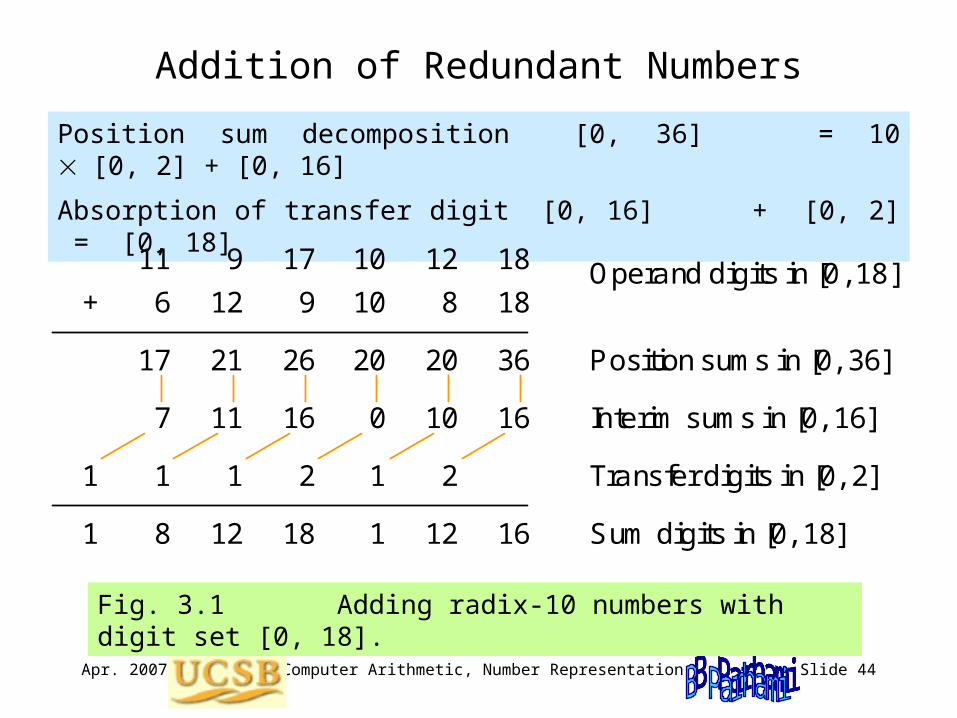
Addition of Redundant Numbers

Fig. 3.1 Adding radix-10 numbers with digit set [0, 18].

Position sum decomposition [0, 36] = 10 [0, 2] + [0, 16]

Absorption of transfer digit [0, 16] + [0, 2] = [0, 18]

6 12 9 10 8 18 Operand digits in [0, 18]

17 21 26 20 20 36

7 11 16 0 10 16

Position sums in [0, 36]

Interim sums in [0, 16]

1 1 1 2 1 2

1 8 12 18 1 12 16

11 9 17 10 12 18


Sum digits in [0, 18]

+


Meaning of Carry-Free Addition

Fig. 3.2 Ideal and practical carry-free addition schemes.

si+1 si–1si

xi–1,yi–1,xixi+1,yi+1yi xi–1,yi–1,xixi+1,yi+1yi

(b) Two-stage carry-free.

si+1 si–1si

ti

(c) Single-stage with lookahead.

si+1 si–1si

xi–1,yi–1,xixi+1,yi+1yi

(a) Ideal single-stage carry-free.

(Impossible for positional system with fixed digit set)

Interim sumat position i

Transfer digitinto position i

Operand digits at position i


Redundancy Index

Fig. 3.3 Adding radix-10 numbers with digit set [0, 11].

So, redundancy helps us achieve carry-free addition

But how much redundancy is actually needed? Is [0, 11] enough for r = 10?

18 12 16 21 12 16 Position sums in [0, 22]

8 2 6 1 2 6

1 1 1 2 1 1



1 9 3 8 2 3 6

11 10 7 11 3 8


+ 7 2 9 10 9 8 Operand digits in [0, 11]

Redundancy index = + + 1 – r For example, 0 + 11 + 1 – 10 = 2


3.2 Redundancy in Computer Arithmetic

Fig. 3.4 Addition of four binary numbers, with the sum obtained in stored-carry form.

0 0 1 0 0 1 First binary number

0 1 1 1 1 0

0 1 2 1 1 1

Add second binary number


+ 0 1 1 1 0 1 Add third binary number





Add fourth binary number


0 2 3 2 1 2

0 0 1 0 1 0

0 1 1 1 0 1

1 1 2 0 2 0

+

1 1 3 0 3 1

1 1 1 0 1 1

0 0 1 0 1 0

1 2 1 1 1 1

+ 0 0 1 0 1 1




Oldest example of redundancy in computer arithmetic is the stored-carry representation (carry-save addition)


Hardware for Carry-Save Addition

Fig. 3.5 Using an array of independent binary full-adders to perform carry-save addition.

Binary Full Adder (Stage i)

c incout

Digit in [0, 2] Binary digit

Digit in [0, 2]

To Stage i+1

From Stage i – 1

x y

s

Two-bit encoding for binary stored-carry digits used in this implementation:

0 represented as 0 0


or as 1 0


Because in carry-save addition, three binary numbers are reduced to two binary numbers, this process is sometimes referred to as 3-2 compression


Carry-Save Addition in Dot Notation

Two carry-save

inputs

Carry-save input

Binary input

Carry-save output

This bit being 1

represents overflow (ignore it)

0 0

0

a. Carry-save addition. b. Adding two carry-save numbers.

Carry-save addition

Carry-save addition

We sometimes find it convenient to use an extended dot notation, with heavy dots (●) for posibits and hollow dots (○) for negabits

Eight-bit, 2’s-complement number ○ ● ● ● ● ● ● ●

Negative-radix number ○ ● ○ ● ○ ● ○ ●

BSD number with n, p encoding ○ ○ ○ ○ ○ ○ ○ ○ of the digit set [1, 1] ● ● ● ● ● ● ● ●

Fig. 9.3 From text on computer architecture (Parhami, Oxford/2005)

3-to-2 reduction

4-to-2 reduction


Example for the Use of Extended Dot Notation

2’s-complement multiplicand ○ ● ● ● ● ● ● ●2’s-complement multiplier ○ ● ● ● ● ● ● ●

○ ● ● ● ● ● ● ● ○ ● ● ● ● ● ● ● ○ ● ● ● ● ● ● ●

○ ● ● ● ● ● ● ● ○ ● ● ● ● ● ● ● ○ ● ● ● ● ● ● ●

○ ● ● ● ● ● ● ● ● ○ ○ ○ ○ ○ ○ ○

○ ● ● ● ● ● ● ● ● ● ● ● ● ● ● ●

Option 2: Baugh-Wooley method

xy

1 x1 1 y

Option 1: sign extension

xx x x x x

Multiplication of 2’s-complement

numbers


3.3 Digit Sets and Digit-Set Conversions

Example 3.1: Convert from digit set [0, 18] to [0, 9] in radix 10

11 9 17 10 12 18 18 = 10 (carry 1) + 811 9 17 10 13 8 13 = 10 (carry 1) + 311 9 17 11 3 8 11 = 10 (carry 1) + 111 9 18 1 3 8 18 = 10 (carry 1) + 811 10 8 1 3 8 10 = 10 (carry 1) + 012 0 8 1 3 8 12 = 10 (carry 1) + 2

1 2 0 8 1 3 8 Answer; all digits in [0, 9]

Note: Conversion from redundant to nonredundant representation always involves carry propagation

Thus, the process is sequential and slow


Conversion from Carry-Save to Binary

Example 3.2: Convert from digit set [0, 2] to [0, 1] in radix 2

1 1 2 0 2 0 2 = 2 (carry 1) + 0 1 1 2 1 0 0 2 = 2 (carry 1) + 0 1 2 0 1 0 0 2 = 2 (carry 1) + 0 2 0 0 1 0 0 2 = 2 (carry 1) + 0


Another way: Decompose the carry-save number into two numbers and add them:

1 1 1 0 1 0 1st number: sum bits + 0 0 1 0 1 0 2nd number: carry bits –––––––––––––––––––––––––––––––––––––––– 1 0 0 0 1 0 0 Sum


Conversion Between Redundant Digit Sets

Example 3.3: Convert from digit set [0, 18] to [6, 5] in radix 10 (same as Example 3.1, but with the target digit set signed and redundant)

11 9 17 10 12 18 18 = 20 (carry 2) – 211 9 17 10 14 2 14 = 10 (carry 1) + 411 9 17 11 4 2 11 = 10 (carry 1) + 111 9 18 1 4 2 18 = 20 (carry 2) – 211 11 2 1 4 2 11 = 10 (carry 1) + 112 1 2 1 4 2 12 = 10 (carry 1) + 2


On line 2, we could have written 14 = 20 (carry 2) – 6; this would have led to a different, but equivalent, representation

In general, several representations may exist for a redundant digit set


Carry-Free Conversion to a Redundant Digit Set

Example 3.4: Convert from digit set [0, 2] to [1, 1] in radix 2 (same as Example 3.2, but with the target digit set signed and redundant)

Carry-free conversion:

1 1 2 0 2 0 Carry-save number–1 –1 0 0 0 0 Interim digits in [–1, 0]

1 1 1 0 1 0 Transfer digits in [0, 1] –––––––––––––––––––––––––––––––––––––––– 1 0 0 0 1 0 0 Answer;

all digits in [–1, 1]

We rewrite 2 as 2 (carry 1) + 0, and 1 as 2 (carry 1) – 1

A carry of 1 is always absorbed by the interim digit that is in {1, 0}


3.4 Generalized Signed-Digit Numbers

Fig. 3.6 A taxonomy of redundant and non-redundant positional number systems.

Radix-r Positional

Non-redundant

Conventional Non-redundant signed-digit

Generalized signed-digit (GSD)

Minimal GSD

Non-minimal GSD

(even r)

Symmetric minimal GSD

r = 2

BSD or BSB

Asymmetric minimal GSD

(r ° 2)

Stored- carry (SC)

Non-binary SB

Symmetric non- minimal GSD

Asymmetric non- minimal GSD

r

Ordinary signed-digit

Minimally redundant OSD

Maximally redundant OSD BSCB

SCB

r = 2

r

Unsigned-digit redundant (UDR)

r = 2

BSC

r – 1r/2 + 1

Radix rDigit set [–, ] Requirement + + 1 rRedundancy index = + + 1 – r


Encodings for Signed Digits

Fig. 3.7 Four encodings for the BSD digit set [–1, 1].

xi 1 –1 0 –1 0 BSD representation of +6s, v 01 11 00 11 00 Sign and value encoding2’s-compl 01 10 00 10 00 2-bit 2’s-complement n, p 01 10 00 10 00 Negative & positive flags n, z, p 001 100 010 100 010 1-out-of-3 encoding

Two of the encodings above can be shown in extended dot notation (● = posibit, ○ = negabit, ■ = doublebit, □ = negadoublebit)

2’s-compl □ □ □ □ □ ● ● ● ● ●

n, p ○ ○ ○ ○ ○ ● ● ● ● ●

These two encodings are nearly equivalent (left-shift the doublebits)


Hybrid Signed-Digit Numbers

i

i

i

i

i

BSD B B BSD B B Type

1 0 1 –1 0 1

+ 0 1 1 –1 1

x

y

1 1 2 –2 1 1

–1 0

1 –1 0

1 –1 1 1 0 1 1

p

w

t

s

BSD B B

–1 0 1

–1 1 1

–1 1 1

0 1 0

–1

0

i+1

Fig. 3.8 Example of addition for hybrid signed-digit numbers.

Radix-8 GSD with digit set [4,7]

The hybrid-redundant representation above in extended dot notation:

n, p -encoded ○ ● ● ○ ● ● ○ ● ● Nonredundantbinary signed digit ● ● ● binary positions


3.5 Carry-Free Addition Algorithms

Carry-free addition of GSD numbers

Compute the position sums pi = xi + yi

Divide pi into a transfer ti+1 and interim sum wi = pi – rti+1

Add incoming transfers to get the sum digits si = wi + ti


si+1 si–1si

tiwi

If the transfer digits ti are in [–, ], we must have:

– + pi – rti+1 –

interim sum

Smallest interim sum Largest interim sumif a transfer of – if a transfer of is to be absorbable is to be absorbable

These constraints lead to:

/ (r – 1)

/ (r – 1)


Is Carry-Free Addition Always Applicable?

No: It requires one of the following two conditions

a. r > 2, 3

b. r > 2, = 2, 1, 1 e.g., not [1, 10] in radix 10

In other words, it is inapplicable for

r = 2 Perhaps most useful case

= 1 e.g., carry-save

= 2 with = 1 or = 1 e.g., carry/borrow-save

BSD fails on at least two criteria!

Fortunately, in the latter cases, a limited-carry addition algorithm is always applicable


Limited-Carry Addition

Example: BSD addition 1 1 1 10 1 0 1

1 1

Fig. 3.11 Example of addition for hybrid signed-digit numbers.

(a) Three-stage carry estimate. (b) Three-stage repeated-carry.

s i+1 s i–1s i

ei

ti

xi–1,y i–1,x ixi+1,y i+1 y i

s i+1 s i–1s i

ti

t'i


(c) Two-stage parallel-carries.

s i+1 s i–1s i

ti(2)

ti(1)


(a) Three-stage carry estimate (b) Three-stage repeated carry (c) Tw o-stage parallel carries

Estimate, orearly warning


Limited-Carry BSD Addition

Fig. 3.12 Limited-carry addition of radix-2 numbers with digit set [–1, 1] using carry estimates. A position sum –1 is kept intact when the incoming transfer is in [0, 1], whereas it is rewritten as 1 with a carry of –1 for incoming transfer in [–1, 0]. This guarantees that ti wi and thus –1 si

1.

1 –1 0 –1 0 x in [–1, 1]

+ 0 –1 –1 0 1

1 –2 –1 –1 1

1 0 1 –1 –1

–1 –1 0 1

0 –1 1 0 –1

i

i+1

y in [–1, 1] i

p in [–2, 2] i

w in [–1, 1] i

s in [–1, 1] i

t in [–1, 1]

low low low high high high

0

0

e in {low: [–1, 0], high: [0, 1]} i


3.6 Conversions and Support Functions

Example 3.10: Conversion from/to BSD to/from standard binary

1 1 0 1 0 BSD representation of +6 1 0 0 0 0 Positive part 0 1 0 1 0 Negative part 0 0 1 1 0 Difference =

Conversion result

The negative and positive parts above are particularly easy to obtain if the BSD number has the n, p encoding

Conversion from redundant to nonredundant representation always requires full carry propagation

Conversion from nonredundant to redundant is often trivial


Other Arithmetic Support Functions

Fig. 3.16 Overflow and its detection in GSD arithmetic.

xk–1 xk–2 . . . x1 x0 k-digit GSD operands + yk–1 yk–2 . . . y1 y0

––––––––––––––––––––––––––– pk–1 pk–2 . . . p1 p0 Position sums wk–1 wk–2 . . . w1 w0 Interim sum digits

⁄ ⁄ ⁄ ⁄ tk tk–1 . . . t2 t1 Transfer digits

––––––––––––––––––––––––––– sk–1 sk–2 . . . s1 s0 k-digit apparent sum

Zero test: Zero has a unique code under some conditions

Sign test: Needs carry propagation

Overflow: May be real or apparent (result may be representable)


4 Residue Number Systems

Chapter Goals

Study a way of encoding large numbers as a collection of smaller numbersto simplify and speed up some operations

Chapter Highlights

Moduli, range, arithmetic operationsMany sets of moduli possible: tradeoffsConversions between RNS and binary The Chinese remainder theoremWhy are RNS applications limited?


Residue Number Systems: Topics


4.1. RNS Representation and Arithmetic

4.2. Choosing the RNS Moduli

4.3. Encoding and Decoding of Numbers

4.4. Difficult RNS Arithmetic Operations

4.5. Redundant RNS Representations

4.6. Limits of Fast Arithmetic in RNS


4.1 RNS Representations and Arithmetic

Chinese puzzle, 1500 years ago:

What number has the remainders of 2, 3, and 2 when divided by 7, 5, and 3, respectively?

Residues (akin to digits in positional systems) uniquely identify the number, hence they constitute a representation

Pairwise relatively prime moduli: mk–1 > . . . > m1 > m0

The residue xi of x wrt the ith modulus mi (similar to a digit):xi = x mod mi = xmi

RNS representation contains a list of k residues or digits: x = (2 | 3 | 2)RNS(7|5|3)

Default RNS for this chapter: RNS(8 | 7 | 5 | 3)


RNS Dynamic RangeProduct M of the k pairwise relatively prime moduli is the dynamic range M = mk–1 . . . m1 m0 For RNS(8 | 7 | 5 | 3), M = 8 7 5 3 = 840

Negative numbers: Complement relative to M–xmi

= M – xmi

21 = (5 | 0 | 1 | 0)RNS

–21 = (8 – 5 | 0 | 5 – 1 | 0)RNS = (3 | 0 | 4 | 0)RNSHere are some example numbers in our default RNS(8 | 7 | 5 | 3):(0 | 0 | 0 | 0)RNS Represents 0 or 840 or . . .(1 | 1 | 1 | 1)RNS Represents 1 or 841 or . . .(2 | 2 | 2 | 2)RNS Represents 2 or 842 or . . .(0 | 1 | 3 | 2)RNS Represents 8 or 848 or . . .(5 | 0 | 1 | 0)RNS Represents 21 or 861 or . . .(0 | 1 | 4 | 1)RNS Represents 64 or 904 or . . .(2 | 0 | 0 | 2)RNS Represents –70 or 770 or . . .(7 | 6 | 4 | 2)RNS Represents –1 or 839 or . . .

We can take the range of RNS(8|7|5|3) to be [420, 419] or any other set of 840 consecutive integers


We will see later how the weights can be determined for a given RNS

RNS as Weighted Representation

For RNS(8 | 7 | 5 | 3), the weights of the 4 positions are:

105 120 336 280

Example: (1 | 2 | 4 | 0)RNS represents the number

1051 + 1202 + 3364 + 2800840 = 1689840 = 9

For RNS(7 | 5 | 3), the weights of the 3 positions are:

15 21 70

Example -- Chinese puzzle: (2 | 3 | 2)RNS(7|5|3) represents the number

15 2 + 21 3 + 70 2105 = 233105 = 23


RNS Encoding and Arithmetic Operations

Fig. 4.1 Binary-coded format for RNS(8 | 7 | 5 | 3).

Arithmetic in RNS(8 | 7 | 5 | 3) (5 | 5 | 0 | 2)RNS Represents x = +5 (7 | 6 | 4 | 2)RNS Represents y = –1 (4 | 4 | 4 | 1)RNS x + y : 5 + 78 = 4, 5 + 67 = 4, etc. (6 | 6 | 1 | 0)RNS x – y : 5 – 78 = 6, 5 – 67 = 6, etc.

(alternatively, find –y and add to x) (3 | 2 | 0 | 1)RNS x y : 5 78 = 3, 5 67 = 2, etc.

mod 8 mod 7 mod 5 mod 3


Mod-8 Unit

Mod-7 Unit

Mod-5 Unit

Mod-3 Unit

3 3 3 2

Operand 1 Operand 2

Result

Fig. 4.2 The structure of an adder, subtractor, or multiplier for RNS(8|7|5|3).


4.2 Choosing the RNS Moduli

Target range for our RNS: Decimal values [0, 100 000]

Strategy 1: To minimize the largest modulus, and thus ensure high-speed arithmetic, pick prime numbers in sequence

Pick m0 = 2, m1 = 3, m2 = 5, etc. After adding m5 = 13: RNS(13 | 11 | 7 | 5 | 3 | 2) M = 30 030 Inadequate

RNS(17 | 13 | 11 | 7 | 5 | 3 | 2) M = 510 510 Too large

RNS(17 | 13 | 11 | 7 | 3 | 2) M = 102 102 Just right! 5 + 4 + 4 + 3 + 2 + 1 = 19 bits

Fine tuning: Combine pairs of moduli 2 & 13 (26) and 3 & 7 (21)RNS(26 | 21 | 17 | 11) M = 102 102


An Improved Strategy


Strategy 2: Improve strategy 1 by including powers of smaller primes before proceeding to the next larger prime

RNS(22 | 3) M = 12RNS(32 | 23 | 7 | 5) M = 2520RNS(11 | 32 | 23 | 7 | 5) M = 27 720RNS(13 | 11 | 32 | 23 | 7 | 5) M = 360 360

(remove one 3, combine 3 & 5)RNS(15 | 13 | 11 | 23 | 7) M = 120 120

4 + 4 + 4 + 3 + 3 = 18 bits

Fine tuning: Maximize the size of the even modulus within the 4-bit limitRNS(24 | 13 | 11 | 32 | 7 | 5) M = 720 720 Too largeWe can now remove 5 or 7; not an improvement in this example


Low-Cost RNS Moduli


Strategy 3: To simplify the modular reduction (mod mi) operations, choose only moduli of the forms 2a or 2a – 1, aka “low-cost moduli”

RNS(2ak–1 | 2ak–2 – 1 | . . . | 2a1 – 1 | 2a0 – 1)

We can have only one even modulus2ai – 1 and 2aj – 1 are relatively prime iff ai and aj are relatively prime

RNS(23 | 23–1 | 22–1) basis: 3, 2 M = 168 RNS(24 | 24–1 | 23–1) basis: 4, 3 M = 1680 RNS(25 | 25–1 | 23–1 | 22–1) basis: 5, 3, 2 M = 20 832 RNS(25 | 25–1 | 24–1 | 23–1) basis: 5, 4, 3 M = 104 160

Comparison

RNS(15 | 13 | 11 | 23 | 7) 18 bits M = 120 120 RNS(25 | 25–1 | 24–1 | 23–1) 17 bits M = 104 160


4.3 Encoding and Decoding of Numbers

Conversion from binary/decimal to RNS

––––––––––––––––––––––––––––– i 2i 2i7 2i5 2i3

––––––––––––––––––––––––––––– 0 1 1 1 1 1 2 2 2 2 2 4 4 4 1 3 8 1 3 2 4 16 2 1 1 5 32 4 2 2 6 64 1 4 1 7 128 2 3 2 8 256 4 1 1 9 512 1 2 2–––––––––––––––––––––––––––––

Table 4.1 Residues of the first 10 powers of 2

Example 4.1: Represent the number y = (1010 0100)two = (164)ten in RNS(8 | 7 | 5 | 3)

The mod-8 residue is easy to find

x3 = y8 = (100)two = 4

We have y = 27+25+22; thus

x2 = y7 = 2 + 4 + 47 = 3

x1 = y5 = 3 + 2 + 45 = 4

x0 = y3 = 2 + 2 + 13 = 2


Conversion from RNS to Mixed-Radix Form

MRS(mk–1 | . . . | m2 | m1 | m0) is a k-digit positional system with weights

mk–2...m2m1m0 . . . m2m1m0 m1m0 m0 1

and digit sets [0, mk–1–1] . . . [0,m3–1] [0,m2–1] [0,m1–1]

[0,m0–1]

Example: (0 | 3 | 1 | 0)MRS(8|7|5|3) = 0105 + 315 + 13 + 01 = 48

RNS-to-MRS conversion problem:y = (xk–1 | . . . | x2 | x1 | x0)RNS = (zk–1 | . . . | z2 | z1 | z0)MRS

MRS representation allows magnitude comparison and sign detection

Example: 48 versus 45(0 | 6 | 3 | 0)RNS vs (5 | 3 | 0 | 0)RNS

(000 | 110 | 011 | 00)RNS vs (101 | 011 | 000 | 00)RNS

Equivalent mixed-radix representations (0 | 3 | 1 | 0)MRS vs (0 | 3 | 0 | 0)MRS

(000 | 011 | 001 | 00)MRS vs (000 | 011 | 000 | 00)MRS


Conversion from RNS to Binary/Decimal

Theorem 4.1 (The Chinese remainder theorem)x = (xk–1 | . . . | x2 | x1 | x0)RNS = i Mi i ximi

M

where Mi = M/mi and i = Mi –1mi (multiplicative inverse of Mi wrt mi)

Implementing CRT-based RNS-to-binary conversionx = i Mi i ximi

M = i fi(xi) M

We can use a table to store the fi values –- i mi entries

Table 4.2 Values needed in applying the Chinese remainder theorem to RNS(8 | 7 | 5 | 3)

–––––––––––––––––––––––––––––– i mi xi Mi i ximi

M

–––––––––––––––––––––––––––––– 3 8 0 0 1 105 2 210 3 315

. . . . . .


Intuitive Justification for CRT

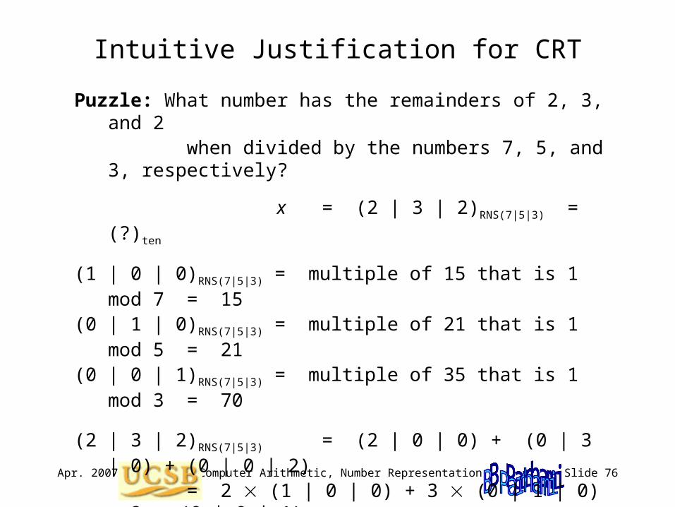
Puzzle: What number has the remainders of 2, 3, and 2 when divided by the numbers 7, 5, and 3, respectively?

x = (2 | 3 | 2)RNS(7|5|3) = (?)ten

(1 | 0 | 0)RNS(7|5|3) = multiple of 15 that is 1 mod 7 = 15



(2 | 3 | 2)RNS(7|5|3) = (2 | 0 | 0) + (0 | 3 | 0) + (0 | 0 | 2)

= 2 (1 | 0 | 0) + 3 (0 | 1 | 0) + 2 (0 | 0 | 1) = 2 15 + 3 21 + 2 70 = 30 + 63 + 140 = 233 = 23 mod 105

Therefore, x = (23)ten


4.4 Difficult RNS Arithmetic Operations

Sign test and magnitude comparison are difficult

Example: Of the following RNS(8 | 7 | 5 | 3) numbers:

Which, if any, are negative? Which is the largest? Which is the smallest?

Assume a range of [–420, 419]

a = (0 | 1 | 3 | 2)RNS

b = (0 | 1 | 4 | 1)RNS

c = (0 | 6 | 2 | 1)RNS

d = (2 | 0 | 0 | 2)RNS

e = (5 | 0 | 1 | 0)RNS

f = (7 | 6 | 4 | 2)RNS

Answers: d < c < f < a < e < b –70 < –8 < –1 < 8 < 21 < 64


Approximate CRT Decoding

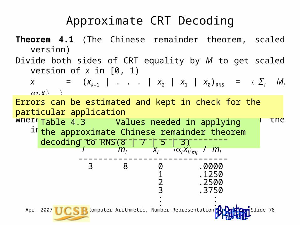
Theorem 4.1 (The Chinese remainder theorem, scaled version)Divide both sides of CRT equality by M to get scaled version of x in [0, 1)

x = (xk–1 | . . . | x2 | x1 | x0)RNS = i Mi i ximi

M

x/M = i i ximi / mi 1

= i gi(xi) 1

where mod-1 summation implies that we discard the integer parts

Table 4.3 Values needed in applying the approximate Chinese remainder theorem decoding to RNS(8 | 7 | 5 | 3)

–––––––––––––––––––––––––––––– i mi xi i ximi

/ mi

–––––––––––––––––––––––––––––– 3 8 0 .0000 1 .1250 2 .2500 3 .3750

. . . . . .

Errors can be estimated and kept in check for the particular application


General RNS Division

General RNS division, as opposed to division by one of the moduli (aka scaling), is difficult; hence, use of RNS is unlikely to be effective when an application requires many divisions

Scheme proposed in 1994 PhD thesis of Ching-Yu Hung (UCSB):Use an algorithm that has built-in tolerance to imprecision, and apply the approximate CRT decoding to choose quotient digits

Example –– SRT algorithm (s is the partial remainder)

s < 0 quotient digit = –1s 0 quotient digit = 0s > 0 quotient digit = 1

The BSD quotient can be converted to RNS on the fly


4.5 Redundant RNS Representations

Fig. 4.3 Modulo-13 adder, with the output and one input being pseudoresidues in [0, 15].

Adder

Adder

x y

z

cout0 0

Drop

Pseudoresidue x Residue y

Pseudoresidue z

Drop Adder

Adder

sum in sum out

Mux

0

2h

operand residue

coefficient residue

h

2h+1

h

–m

LSBs

h

2h h

h2h

MSB

0 1

Sum out Sum in

Operand residue

Coefficient residue

Fig. 4.4 A modulo-m multiply-add cell that accumulates the sum into a double-length redundant pseudoresidue.

[0, 15] [0, 12]

[0, 15][0, 11]

if cout = 1

[0, 15]


4.6 Limits of Fast Arithmetic in RNS

Known results from number theory

Implications to speed of arithmetic in RNS

Theorem 4.5: It is possible to represent all k-bit binary numbers in RNS with O(k / log k) moduli such that the largest modulus has O(log k) bits

That is, with fast log-time adders, addition needs O(log log k) time

Theorem 4.2: The ith prime pi is asymptotically i ln i

Theorem 4.3: The number of primes in [1, n] is asymptotically n / ln n

Theorem 4.4: The product of all primes in [1, n] is asymptotically en


Limits for Low-Cost RNS

Known results from number theory

Implications to speed of arithmetic in low-cost RNS

Theorem 4.8: It is possible to represent all k-bit binary numbers in RNS with O((k / log k)1/2) low-cost moduli of the form 2a – 1 such that the largest modulus has O((k log k)1/2) bits

Because a fast adder needs O(log k) time, asymptotically, low-cost RNS offers little speed advantage over standard binary

Theorem 4.6: The numbers 2a – 1 and 2b – 1 are relatively prime iff a and b are relatively prime

Theorem 4.7: The sum of the first i primes is asymptotically O(i2 ln i)


si+1 si–1si

xi–1,yi–1,xixi+1,yi+1yi xi–1,yi–1,xixi+1,yi+1yi

(b) Two-stage carry-free.

si+1 si–1si

ti

(c) Single-stage with lookahead.

si+1 si–1si


(a) Ideal single-stage carry-free.

(Impossible for positional system with fixed digit set)

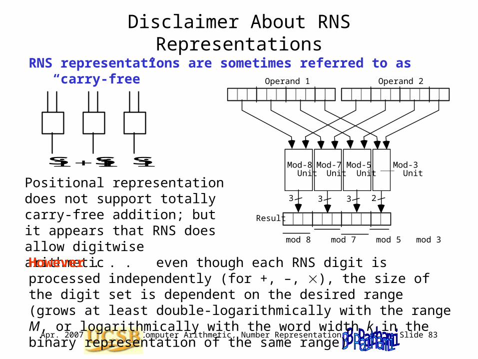
Positional representation does not support totally carry-free addition; but it appears that RNS does allow digitwise arithmetic

Disclaimer About RNS Representations

RNS representations are sometimes referred to as “carry-free”

However . . . even though each RNS digit is processed independently (for +, –, ), the size of the digit set is dependent on the desired range (grows at least double-logarithmically with the range M, or logarithmically with the word width k in the binary representation of the same range)


Mod-8 Unit

Mod-7 Unit

Mod-5 Unit

Mod-3 Unit

3 3 3 2

Operand 1 Operand 2

Result

Apr. 2007Computer Arithmetic, Number RepresentationSlide 1 Part I Number Representation.

Documents

Transcript of Apr. 2007Computer Arithmetic, Number RepresentationSlide 1 Part I Number Representation.