apps.dtic.milr --I Report No FAA-RD-7H3 ~ ~~ AVIATION AUTOMATED WEATHER OBSERVATION SYSTEM (AV-AWOS)...
132
AD A072 119 NATIONAL WEATHER SERVICE SILVER SPRING MD F/G /2 — AVIA TION AUTOMATED WEATHER OBSERVATION SYSTEM CAV—AWOS).(U) MAR 79 DOT—PAY3WAI—3fl UNCLASSIFIED FAA—RD 79—63 Pt _ U - 1 ~~~~~~~~ UUI ~ flU -- B p
Transcript of apps.dtic.milr --I Report No FAA-RD-7H3 ~ ~~ AVIATION AUTOMATED WEATHER OBSERVATION SYSTEM (AV-AWOS)...

AD A072 119 NATIONAL WEATHER SERVICE SILVER SPRING MD F/G /2— AVIA TION AUTOMATED WEATHER OBSERVATION SYSTEM CAV—AWOS ).(U)
MAR 79 DOT—P AY3 WAI—3flUNCLASSIFIED FAA—RD 79—63 Pt
_ U-
1~~~~~~~~ U U I ~flU --
B
p
10______ ~ 3~ S
— iim~~I I ~ 2 O1• i : tUll~~
1111 125
NATIONAL BUREAU oc ST*N~~RQ$

r --
IReport No FAA-RD-7H3
~~~
AVIATION AUTOMATED WEATHEROBSERVATION SYSTEM (AV-AWOS)
National Weather ServiceNatienal Oceanic and Atmospheric Adinkilstratise
Deportment of Commerce C) ‘k:::
o~0$ 4V ts O~
March 1919>- Final Report
Document is ova l ithie to the U.S. public throughthe National Technical Information Service ,
Springfie ld , VIrginia 22161 .
Prepared for
U.S. DEPAR TMENT OF TRANSPORTAT IONFEDERAL AVIAT~N AOMV4ISTRATION
Systems Research & Deveiopm~tt ServiceWashkigton, D.C. 20590
flj (VI 119__________________________ - ~~~~~~~~ -- —
-
~~~~~~~~~~ ~~~~~~~~~~~~~~~ ____ _____

This document is disseminated under the sponsorshipof the Department of Transportation in the interestof information exchange. The United States Govern-ment assumes no liability for the contents or usethereof.
~~~~- - -_ _ __ _ _ _1 — -. ~::—~~~~ ~~W L~~~ ~ __________

- T.chnicol R.pors Docum.ntasion Pog.
I. R.port o~ /, --
2. Gor.r nm .nt A cc.ss i on No. 3. R.c~p1.nt s Cata log Ne.
4. TitI . and Su bt i t le ~~~. Rgpo r ’ Dot.
- - - ~ . Marc~~1979 JAviation Automated Weather Observation System / - 6. P.rfor m ng Orgo n igat on Code(
~ (AV-AWOS )~ —
~~~~~~~
I —
8. Perfo $~~~ b~gjinjiir~ ~—~si~’t No.7 . A ut or ’ s) ( / -
9. Performin g Organ izat ion Nams and Addr es s 10 Work Un it No. ( T R A I S ) -
Na tiona l Weather Service 153—4518.~6O 13th Street
1 1 . Ctt ntract or Grant Na.
Silver Spring , Maryland 2O9l~.- IAA DOT FA73WAI—384 ‘
~~~
13. lype o f Repor t arid Pe riod Cov .r,d
12. Sponsoring Agency Name and Add ’.,. N -U.S. Department of Transportation / ,~
—
Federa l Aviation Administrati on / Fina l .
Systems Research and Development Service ~~~~~ 14 . onso r ng A g.ncy Code
~~ Washington, IJC 20590 —
ARD—450
I 15. Supp lem .nta ry Not es
- ‘7 ~ \AJ r~ — 3 -.~ -•
- -
~~~~~~~-
~~~~~~~~~~~~~~~~~~~~~~
16 A b.t ract
The test results of the Aviation Automated Weather Observation Sys tem(AV—AWOS) at Newport News , Virginia , are presented. The rationalefor the cloud and visibility algorithms is discussed . Verificationof these algorithms is presented . The algorithms for convertingsensor data to automated observations of cloud height , sky cover ,and visibility are specified . Tabulation of the user reactions toan automated observation is presented .
-
17. Key Word. 15. Distr ibution Stet.m.nt
Automated Weather Observations , Document is available to the U.S.AV—AWOS public through the Nat iona l Technical
Infprmation Service , Springfield , VA
_ _ _ _ _ _ _ _ _ _ _ _ _ _ _ _ _ _
22~~’l.
19. Secu ri t y Clo ss i f. (of thu report) 20. S.cu,lty CIeseiI. (of .1,1. pig.) 21. 14.. of Peg.. 22. Pri ce
UNCLASSIFIED UNCLASSIFIED 131
Form DOT F ~1OO.7 (~~ 12) Re,roductuon of comp l.,.d pog. out horlisd ~
:
~
-:
~
/
- - ~9 ~~~~~~~~~ ~~~~~~~ _
— 7 - ~~~
-. -
- r - -- .- ----- -•- — — • -~~
--~.--
~--. -.--- - - •---- . --—..--— ... • — . -.---—--- — — --—
~-—-
~~---—--- -~~~~~~ L_~~~~~ - ~
—~~
‘—— ‘-—~~~~~~ .. .
it~ g ~
II -~~~~
~
Ihui Uli Iii P ~
~~~~~~~~~~~~~~~~~~~~~~~~~~~~~~~~~~~~~~~~~~ :~~~~~~~~~ -~~ 5 . ~
~~~~~~~~~~~
~iI~ iiI~ 2
~~ s~~ 2 .1 j _ Y.
u ii Ig ii St LI SI ii Pt rt It DI $ S ~ S S P £
i i I(fl 1111 101 1111 11111111 (01 101 110 III llHfihll HO III 101 1 11111111111 111 101 1111 101 HI 11111111 1111101 11111111 111 101 1111 11111011 HIt fi l l 1111 1111 110 DII DII OIl 101 1111 111111 111
~ ~1I’’
~,I’I’,
~’ I’ f 1, I’ 1~1t (’
~ II ‘~1~t’r I’I’l’~1’I’1 ~I’ ~~~~~~~ ] 1 i’1] ~~
t ilt ~~~~~~~
~ •(~t jilitil
J ~~~~~~~~~~ ~~ b’~ 2 .2~ j i~~ — — - - Y ’ p .~
I ~ 1111 11111 di j I
I - IS
~~ :!:~: _ ~III Jill ~ ~~1~i1 UUi I i i~ IhtIflH 1~
J ig~~~I “i~~”II
5-
— ~~~~~~~~~~~ ~~~~~~~~~~~~
— -~~
—.~~---~~~~~~~~ .— — -~ —‘~-—~~~~
--‘~~~~~~~~~ -.- ——

• AV-AWOS EXECUTIVE SUMMARY
In June of 1.973 a program to develop an Aviation AutomatedWeather Qbservation ~ystem (AV—AWOS) was Initiated underInteragency Agreement DOT—FA 73WAI--394 between the NationalWeather Service (NWS) and the Federal Aviation Administration( FAA) .
- - At that time most of the weather parameters could be observed
automatically , however , the most important parameters of an aviationweather observation——clouds , visibility and present weather , e. g. ,hail , freezing rain , thunderstorms , still required a subjectivejudgement of an observer.
The major emphasis of the AV—AWO S development was directedtoward solving the cloud and visibility problems and the integrationof these e f fo r t s into an automated station .
• The technical approach involved the definition and requirementsof an AV—AWO S system. This included the design and selection of
— best available sensors , development of processing algorithms , hardwaredesign of sensor interfaces , the processing functions and the outputcommunications . The AV—AWO S system would be tested at a medium sizedairport which was at N ewport News , Virginia (PHF) . This operationaltest was evaluated for the acceptance by users and for the acceptanceof the automated report as a certified weather observation.
Several significant contributions have been realized duringthis program. Some of the most important are as follows:
a) A determination of the magnitude of the requirements fora totally automated station.
b) The development of the initial sensor processing algorithmsof the subjective type of weather observations.
c) The investigation into several types of sensors for variousweather parameters.
d) The intensive investigation into the laser ceilometerstatus, which indicated the true status of such sensors.
e) The initiation of the development of utilizing a lasersensor for present weather indicators (such as fog , snow,rain, etc.).
H
i i i

f ) The internal error checking and data quality controlfunct ion usually performed by an observer.
g) What the aviation public objected to and what they applaudedin an automated observation .
h) Realizing all of the above factors , realistic nodels havebeen developed utilizing the latest electronic technologies(micrnprocessors) to produce a sore economical and sorereliable totally automated system . -
The AV—A*)S program pointed out many of the major deficienciesin all aspects of developing totally automa ted systems. This haslead to intensified programs within NWS , FAA and other agencies inthe development of ceilometers, visibility and present weathersensors realizing what is truly requ ired for aviation services .
Even tkz~ugh the major part of the AV-AWOS program is completedit ii still planned to use the remaining fund s to support someevaluat ion efforts required with these new sensors as they becx me
• available. -
This report covers the final phases of the AV-AWOS program andincludes technical information required to system specifications anduser evaluation results from the Patrick Henry tests.
F —
iv
I__ ~~~ 2 ...~i ~~~~~~~~~~~~~~~ ~~~~~~~~~~~~~~ -~~ ~~~~~~ v ~~~~~~ ‘ ~~~~~~~~ - . _________
- -•~~~j .
- —

-
-—-
~~~~~~~~~~~~~~~~~~~~~~~~~~~~~~~~~~~~~~~~~~~~~~~~~~~~~~~~~~~~~~~~~~~~~~~~~~~~~~~~~~~~~~~~~~~~~~~~~~~~~~~~~~~~~~~~~~~~~~~~~~~~~~~~~~~ I
TEST AND EVALUATION DIVISION REPORT NO. 2—78
AUTOMATING CLOUD AND VISIBILITY OBSERVAT IONS
James BradleyMatthew Lefkowitz
Richard Lewis
OBSERVATION TECHN IQUES DEVELOPMENT AND TEST BRANCHTEST AND EVALUATION DIVISIONOFFICE OF TECHNICAL SERVICES
STERLING RESEARCH AND DEVELOPMENT CENTER- STERLING , VIRGINIA 22 170
• ACC0~~_____
\ DC~~~~~~F NOVEMBER 1978 ~~~~~~~~~~~~~~~~~~~~~~~~
rI
~~~~~~~~~~~~~~~~~
\D%s~~,~\
s~ec\3.
-- -~ - -~~ - - ---.
• - - ~~
~A ~~~~~~~~~~~~~~~~~~~~~~~~~~ - - -

r ~~~~
—---- -— ---
~~~~
- -
~~~~
- ---
~~~~~~~
MANAGEMENT SUIIMARY
AV—AWOS is the acronym for Aviation Automated Weather Observation
~ystem . The overall system is designed to totally automate the aviationsurface weather observation. The work element discussed in this reportdeals only with the development and test of methods for automated observingtechniques for cloud heigh t , sky cover and visibility. This report is in-tended to be part of a specification prepared by the Equipment Development
• Laboratory (part of the National Weather Service ’s Systems DevelopmentOff ice) fo r the Federa l Aviation Administration .
Programs for the development of automated observing techniques havebeen conducted fo r several yea rs by the O f f i c e of Techn ical Services ’ Testand Evaluation Division. Algorithms for automated observations of sky andvisibility have been conceived based on a relatively small data sample froma sensor network surrounding Dulles International Airport. During theperiod January to May 1978, f ully automated weather observations were usedin an operational test at Patrick Henry International Airport, Newport News,Virginia. There, the automated observations were compared with routine ob—servations made by the duty f l ight service specialist. Test results showedfavorable comparisons with the observer. Several weaknesses were noted ,
r almost exclusively, related to sensor performance.
The cloud and visibility algorithms are considered operative. Thisreport specifies the manner in which the algorithms can be used , and theirlimitations.
The results of the development and test of the automated observingtechnique can be summarized as follows:
• Visibility Observations
— The operational definition of visibility focuses on thehuman observer. Human observations of visibility , however ,have many limiting factors . For example , point of obser—vation, and the nature and number of visibility markersimpart unique characteristics to each observation.
— The visibility sensor used in these tests (Videograph) hasa limited sampling volume : 13 f t . 3. The unit , however ,samples a relatively large volume compared to other typesof single—ended visibility sensors currently marketed.Because of this volume, “grab” samples of 2 to 30 perminute show no significant difference s when averagedover a time period of 6 to 10 minutes.
I
j

—-~~~- • - ~~~~—~~~~- - - -~~~~~--- - ~~~~~~~~~~~ -~~--~~~
MANAGEMENT SUMMARY (Continued)
— When using three visibility sensors, sensor derived prevail-ing visibility had only fair agreement with human visibilityduring these tests. ~4e believe this to be related to thelimitations of subjective observing techniques, differencesbetween human and automated concepts of observing , and re-actions of the Videograph during certain obstruction tovisibility situations.
— The inability of a single visibility sensor to report sectorvisibility may be a limitation in some operational applica-tions. But with appropriate processing , a single sensor canproduce a useful index of v is ib i l i ty . By de f in ition , a singlesensor could never report prevailing visibility. It could beused to report “station” visibility at smaller or limitedservice airfields.
Cloud Observations
— The operational definition of sky condition is based on thepresence of a human observer with inherent limitations.
— Test results show that our computer—generated observationsare in agreement wi th human observations . Our data sampl—ing, averaging times and network configuration , while notunique, are appropriate for use in automated surfaceobservations.
— Our program for observing total and par t ia l obscurations ismarginal. No sensors are currently available that measurethe amount of sky obscured or vertical visibility into an
• obscuration. Until such equipment is developed , adequatealgorithms for partial and total obscurations cannot begenerated . Our algorithms for obscurations are the weak-est part of our program. Under some combinations of weatherconditions, unrepresentative observations of obscuration canbe output by the automated system.
— The three sensor cloud algorithm shows good agreement withhuman observations. Variances are largely related to dif-ferences in human and automated concepts of observing.
— The inability of a single cloud sensor to report directionalbias cloud remarks may be a limitation in some operationalapplications. Our tests, however , shoved excellent agreement —
between two separated single sensors as well as between net—work and single sensor observations.
ii
— ~~~~ • • . ----- ~-- .:~:::. •. — - ~~~~~~~~~~~~~~~~~~~~~~~~~~~ ~~~~~~~~~~ -

MANAGEMENT SUMMARY (Concluded)
Network Size and Siting
— If prevailing v isibility is required , three visibility-
, sensors are needed — more , if there are unusual localproblems . In normal situations , the three sensorsshould be installed at the vertices of an equilateraltriangle having approximately three mile legs. Therequired point of observation should be at the triangle’scenter.
— If an index of visibility is required , one visibility• sensor is needed — more , if there are local visibility
problems.
— In most situations , one ceilometer would be adequate.More would be needed if directional bias is present.
• If three ceilometers are needed for more representa-tive information , they should be installed at the
• vertices of an equilateral triangle having 6 to 8mile legs. The required point of observation shouldbe at the triangle ’s center.
— We do not believe that the algorithm test resultswould be affected by small changes in networkconfigurations.
— Installation of an automated weather system shouldproceed in a manner typical of other major aviationfacilities. This includes an initial period of inves-tigation to define the required network configuration .Continued review , after commissioning, is also needed .
iii
.—~-
~~~~~—
~~~~-——----—-—‘
~~~~~~~~~~~~~~~ ~~~~~~~~~~~~ -
-~ —~~~~
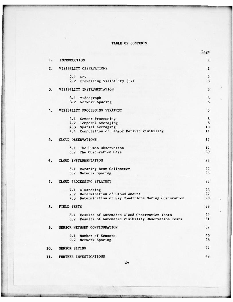
• TABLE OF CONTENTS
Page
1. INTRODUCTION 1
2. VISIBILITY OBSERVATIONS 1
2.1 SEV 2• 2.2 Prevailing Visibility (PV) 3
3,. VISIBILITY INSTRUMENTATION 3
3.1 Videograph 33.2 Network Spacing
4. VISIBILITY PROCESSING STRATEGY 5
4.1 Sensor Processing 84.2 Temporal Averaging 84.3 Spatial Averaging 104.4 Computation of Sensor Derived Visibility 14
5. CLOUD OBSERVATIONS 17
5.1 The Human Observation 175.2 The Obscuration Case 20
6. CLOUD INSTRUMENTATION 22
6.1 Rotating Beam Ceilometer 226.2 Network Spacing 23
7. CLOUD PROCESSING STRATEGY 23
7.1 Clustering 237.2 Determination of Cloud Amount 277.3 Determination of Sky Conditions During Obscuration 28
8. FIELD TESTS 28
8.1 F~esults of Automated Cloud Observation Tests 298.2 Results of Automated Visibility Observation Tests 31
9. SENSOR NETWORK CONFIGURATION 37
9.1 Number of Sensors 409.2 Network Spacing 46
10. SENSOR SITING 47
11. FURTHER INVESTIGATIONS 49
iv
~~~~ - —-~~~~~~~ ~~~~~~~~~~~~~~~~~~~~~~~~~~~~~~~~~~~~~~~~~~~~~~~~~~~~~~~~~~~~~~~~~~~~~~~~~~~~

- ~~~~~- T:: -
TABLE OF CONTENTS (Concluded)
-j -
12. SUMMAR Y Si
-~ • 12.1 Visibility Observations 51
12.2 Cloud Observation Automation 52
-~~ 12.3 Network Size and Siting 53
13. ACKNOWLEDGMENTS 54
-~ 14. REFERENCES 54
- - APPEND iX A : VISIBILITY ALGORITHM A—i
APPENDIX B : CLOUD ALGORITHM B—i
APPENDIX C: AV-AWOS USER ASSESMENT PLAN RESULTS C l
v
- -- .-~~~~~~~~~~ -- . - , . ,—_~ ---~ -
L. ~~~~~~~~~~~~~~~~~~~~~~~~~~~~~~~~~~~~~~~~~~~~~~~~~~~~~~~~~~~~~~~~~~~~~~~~~~~~ -~~~~- - - - -~~~~~~~~~~
- - -

—~~~~~~
LIST OF FIGURES
Page
Figure Number
1 AV—AWOS Test Network at Dulles InternationalAirport , Chantilly, Virginia 6
2 AV—AWO S Test Network at Patrick Henry InternationalAirport , Newport News, Virg inia 7
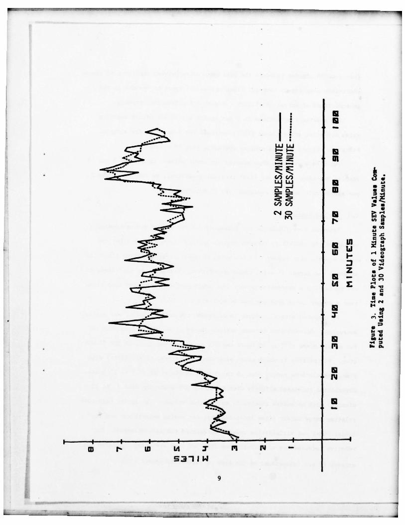
3 Time Plots of 1 Minute SEV Values Computed Using 2and 30 Videograph Samples/Minute 9
4 Time Plots of SEV Averages Over 6 and 10 Minutes 11
5 Time Plots of 6 Minute SEV Derived from 2 and 30Videograph Samples/Minute 12
6 Time Plots of 10 Minute SEV Derived from 2 and 30Videograph Samp les/Minute 13
7 Time Plots of 10 Minute SEV at 3 Locations in PHFNe t 15
8 Network PV Computed Using SEV ’s from Figure 7 16
9 Packing Effec t 19
10 Example of Hierarchical Clustering 25
11 Minute—by—Minute Plot of the Lowest Cloud Returnsfrom RBC Site 7 Miles NE of PHF , Apr i l 26 , 1978 26
12 Visibility Site Locations at Newport News 36
13 Disbribution of Remarks for Clouds and Visibility atEach Sensor Site at PHF 45
vi
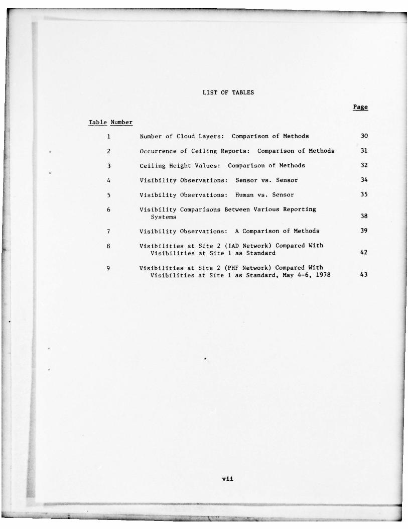
LI ST OF TABLES
Table Number
- • 1 Number of Cloud Layers: Comparison of Methods 30
2 Occurrence of Ceiling Reports: Comparison of Methods 31
3 Ceiling Height Values: Comparison of Methods 32
4 V i s i b i l i t y Observations : Sensor vs. Sensor 34
5 Visibility Observations : Human vs. Sensor 35
6 Visib ili ty Comparis ons Be tween Vario us Repor tingSystems 38
7 Visibility Observations : A Comparison of Methods 39
8 V i s i bi li t i e s at Site 2 ( lAD Network) Compared WithV i s i b i l i t i e s at S i te 1 as Standard 42
9 Vis ibil i t i e s at Site 2 (PHF Network) Compared WithVi sib ili t ies at S i t e 1 as Standard , May 4—6 , 1978 43
vii
- ~~~~~ ~~~~~~~~~~~~~~~ - - - -~~~~~
--~
. .~~~~

1. INTRODUCTION
AV—AWOS is the acronym for Aviation Automated Weather Observation ~ystem.
The overall system is designed to totally automate the aviation surface
weather observation . The work element discussed in this report deals only
with the development and tests of methods for automated observing techniques
• for cloud height , sky cover and visibility. This report is intended to be
part of a specification prepared by the National Weathe r Service ’s Equipment
Development Laboratory for the Federal Aviation Administration.
Cited in this report is the rationale for the algorithm s, and test
results at two airport locations . An important feature is the discussion
of automated observation limitations due, in part, to instrument deficiencies.
Othe r sections include information on sensor network configurations and how
siting requirements should be determined . Finally, the algorithms by which
sensor input is converted to automated observations of cloud height , sky cover
and visibility are specified in the appendices .
2. VISIBILITY OBSERVATION S
Federal Meteorological Handbook #1 (FMH—l) (NOAA—Nation a l Weather Service ,
1970) describes three types of visibility observations: runway visual range
(RVR ) , runway visibility (RVV), and prevailing visibility (PV) . The first
two are highly specialized and have an accepted method of derivation from
transaissometer measurements (Lefkowitz and Schlatter , 1966). The third type
(PV) is based on the subjective visual impressions of a human observer scan-
ning the apparent horizon . By using the technique of “sensor equivalent
visibility” (SEV), developed by George and Lefkovitz (1972), we have been
able to process measurements from a network of sensors to produce an equiva-
lent of PV.
1
• - - • ‘

-•--—- -— -—• ---—- -- - -
Prevailing visibility is the most d i f f i cu l t subjective observation para-
meter to automate. Attemp t ing to put an individual ’s visual impressions in
logic form is ambitious. The basic types of visibility sensors available
today are a limiting factor. Most measure within a limited sampling volume.
This spot measurement is extrapolated to larger volumes with the assumption
of homogeneity (George and Lefkowitz , 1972; Chishoim and Kruse , 1974b) .
One purpose of the tests was to use limited sampling sensors in the
development of automated PV. We tried to satisfy the space averaging require-
ments of PV by employing a three sensor network with appropriate data process-
ing. Time averaging was also an input to sensor derived PV. We also tested
to determine the feasibili ty of using only one sensor as an index of PV (for
use at limited service locations) .
In this report, we describe techniques used for determining time averages
and data sampling rates for sensor PV. While these averages were developed
using a specific sensor type, the techniques are generalized and will apply
to most visibility sensors.
2.1 SEV
SEV is defined as any equivalent of human visibility derived from in—
strumental measurements. In practice , the sensor from which SEV was derived
required uniform visibility for an accurate calibration . Once calibrated ,
a sensor was then used to determine visibility under all conditions.
In our experiments, sensor visibility was measured by a backscatter
sensor. This instrument relates visibility to the amount of projected light
reflected back into the detector by particles in the air. The output of this
instrument is converted to Sty by using an empirical relationship established
by Hochreiter (1973). While backscatter sensors were used in our tests, a
SEV calibration can be developed for any type of visibility sensor.
2
~~~~~~~~~~~~~~~~~~~~~ .4

- -•~~~~~ ----~~~~~~~ - - -~~~~~~~~~~~~~ - - -- ----~~~---- • - - - -
~~~~~~~~~~~
-
~~~~~~~~~~~~~
---- - -
~~~~~
-
~~~~~
-
2.2 Prevailing Visibility (PV)
FMH— l specifies the manner in which human observations of visibility
are to be taken and reported. It defines PV as , “The greatest visibility
equaled or exceeded throughout at least half of the horizon circle which
need not necessarily be continuous.” PV is determined at either the usual
site(s) of observation or from the control tower level.
SEV and PV have different principles of observation. SEV is based on
• measurement of a small volume sample with extrapolation to overall areal
visibility. PV, as determined by a human, relies on sensory information
integrated over a relatively extensive area. SEV, based on a point sensor,
usually has strongest relationships with PV during homogeneous conditions.
It is important to note that the definition of PV, written for human observers
as it is, could very well require an infinite number of sensors for automation
to duplicate the human observation; however, practical and economic consid-
erations dictate the use of as few sensors as will supply a useful product.
3. VISIBILITY INSTRUMENTATION
The ideal visibility instrument should have a direct relationship to
the characteristics of human visibility. To our knowledge, such a sensor is
not available for field use. The Videograph was selected for the visibility
tests because it was readily available, was capable of field operation with
little maintenance and had a traceable calibration.
3.1 Videograph
The Videograph is a backacatter visibility sensor. The instrument con—
sists of a projector and receiver contained in a single housing mounted on a
pedestal. The projector uses a xenon lamp that emits high intensity, short
duration (1 us) pulses of blue—white light into the atmosphere at a 3 Hz
3
L~~ ~~~~~~~~~~~~~~~~~~~~~~~~~~~~~~~~~~~~~~~~~~~~~~~~~~~~~~~~~~~~~~~~~~~~~~~~~~~~~~~~~~~~~~~~ ~~~~~~~~~~~~~~~ --~~~ -.- -~~~ - - --- - -~~~~~~~~~~~~ -- -

rate. The receiver measures the amount of projected light scattered back
into a detector by particles in the atmosphere. The detector uses a reverse—
biased PIN silicone photodiode. The Videograph output ranges from 0 to 999
MA with a system time constant of about 3 minutes .
The optical axis of the projector is inclined upwards at 30 so that it
intersects the horizontal axis of the receiver optics at 17 feet. The com-
mon volume of the system extends about 600 feet from this point of inter-
section, although most of the backscattering occurs within the first 5 to
100 feet (Curcio and Knestrick, 1958). Using the 100—foot sampling length,
the volume of atmosphere that can be sampled at any one tine is about
13 ft.3.
The ~A output of the Videograph detector is converted to SEV using the
empirically determined curves described by Hochreiter (1973). He established
two conversions from pA to SEV values: one for daytime use and one for night.
The values are:
Visibility Day pA Night pA
1/4 mi. 900 9991 ml. 470 5302 ml. 340 3803 mi . 280 3105 mi. 220 2507 ml. 190 210
Conversion equations can also be developed for different types of
obstruction to vision (Sheppard, 1977). In our work, however , we did not
differentiate between different obstructions to vision.
The Videographs are calibrated against a collocated standard Videograph
which is referenced against human visibility. Using paired measurements of
sensor vs. standard, these data are grouped into classes ranging from 1/4
mile to 7 miles. Within each class, the mean difference between the sensor
4
~~~~~~~~~
-•—~~~~----~~~~~~~~
- —~~~~~
and standard must be less than 10% of the standard’s output for the sensor to
be considered calibrated. We checked the Videographs used at PHF before and
after the four—month operational test. All had stayed within the alloted
+ 10%.
3.2 Network Spacing
The length of each leg in our visibility triangle for both LAD and PHF
tests was about 3 miles with a Videograph located at each vertex: the human
observer was at the nominal center (Figures 1 and 2). Since visibility is a
fragile parameter subject to small scale temporal changes and physical modi-
fication, the network was kept relatively small. The decision to use 3—mile
legs was predicated on the need to supply the aviation coimnunity with visi—
bility information over a large area around an airport while keeping within
the same visibility universe. Use of three sensors was a pragmatic choice
based on resources, difficulties in obtaining sites and complexity of in-
stalling data lines across great distances. A more comprehensive method might
have been to test many sensor arrays of varying size. Economic and time
constraints doomed that approach. We feel our network is appropriate for
determining PV, but we do not believe it is unique.
4. VISIBILITY PROCESSING STRATEGY
Processing strategies for de’termining PV using a network of sensors ~ iat
take into account the temporal and spatial variability of the atmosphere, as
well as the characteristics and sampling volume of the sensor in use. In the
subsequent paragraphs, we assess the role of these factors in developing a
technique that will be sensor independent.
5
~~~~~~~~~~~~~~~~~~~~~~~~~~~~~~~~~~~~~~~~~~~~~~~~~~~~~~~~~~~~~~~~~~~~~~~~~~~~~~~~~~~~~~~~~~~~~~~~~~~~~~~~~~~~~~~ ~~~~~~~~ - J

F..
zU ) U
~~~~~ A.o x ~ci.~~~w z o.4 .4 ~2
I‘I hi
‘ I/‘C’,
‘ Ao /
.4 f CiLU c~~I I
/ ‘S0 ~
•~~.
uJ I I ~p O~~~l
&,_~~~~~ ‘, •II • ‘~ol— F- / ~ ‘
is I C:) Ij’ b. F1~~~
0o / .5. IIL (f~
F Iv1-4
LU / l~~..2
LU I ,....~
I—. I_~o
-‘ I 1—i l-..hi n O ) P -
I 0I
‘p.~~~~~‘ I C-,
II
•44 ~
-~~~C~ 1 h i-I.’
‘ p 5 1.-I
CiF~o~~~ 1-’ .Cg.~ ~-4 U~~~CI)
* —u~~zu;z~~o x o w~~t n O . 4 I •4 0 . 4<~a s 5 p .~~~Il) < . s .4 ZF... U-4 V) 0~~~ C~~~ U~~~0~~~~0
C-) .-4 C~ P ~~~ .-l N• i ~~~ L) C-) U )-4 >~~~~~~~~~
6
• -‘-- - ~~~~~~~~~~~ _• _•~~~~~~~~~~~~~~~~~~ _ ~~~~~~~~~~~~~~~~~~~~~~~~~~~~~~~~~~~~ -
~~~

N 2
V2
...••• ‘ii
E.VI az:,, FSS \
1
C 1 •
~
ls*s
**......
-
. C3
RBC SITES VIDEOGR.APH SITES
Cl — Ft. Eustis Vi — Denbigh
C2 — Seaford V2 - Kentucky Farms
C3 - BOMARC V3 - Hampton Roads Academy
NEWPORT LIEWS AV-AWOS SITES
Figure 2. AV—AWOS Test Network at Patrick Henry
International Airp ort , Newport News , Virginia
• 7
_ _ _ _ _ _ _ _ _ _ _ _ _ _ - ~~~~- ~~~~—..—I,— —
•.— — —

— - ----- - - --•--- - — - - -- —~~~- • • - -•--- •—• —---•--.
4.1 Sensor Processing
The output of the Videograph detector is designed to oscillate over a
range of 2% of full scale (999 pA) as the amplifier searches for equilibrium.
With our data collection system recording the output of the detector every 2
seconds, we are able to check the Videograph design criteria. Analysis of
data sets taken during various periods of uniform visibility shoved tha t , in
each episode, the data samples fell within a 10 to 15 pA standard deviation
(S.D.) about the mean detector output. These values of S.D. are well within
the design criteria and also confirm the work of Hochreiter (1973) and Shep—
pard (1977).
Under uniform visibility conditions, we computed Sty using sampling rates
-
• varying from 2 to 30 samples per minute. As expected , the number of samples
averaged had little effect upon the computed SEV. Thus, under uniform vlsi—
bility conditions, computation of Sty is independent of sampling rates.
4.2 Temporal Averaging
During varying visibility conditions, SEV is more dependent on the sampl-
ing rate. Figure 3 shows an example of one—minute SEV using two different
processing schemes. One curve was constructed using successive one—minute
averages of SEV computed from Videograph samples of two per minute: resultant
pA values have been linearly averaged. The dotted curve shows a SEV compu-
tation for the same data period using 30 samples per minute.
Short—term averaging, over one—minute for example, emphasized the non-
homogeneous nature of the small volume visibility measurements. Human ob—
servers tend to integrate these characteristics. In order to emulate human
methods and provide a more appropriate observation, we tested various averag-
ing schemes from 5 to 20 minutes. We concluded that averaging intervals of
8
-
~~~~~~~~~~ - - - —-- - - -~~~- - - -- .
- ~~~~~‘~~~—.
~~~~~~~- - •
- . ~~~~~~~~~~~~~~~~~~~~~~~~~~~~ ~~~~~~~~~~~~~~~~~
C —. -— - --r-n - - - - 7r - -
m,5~~~, m-4 -.
“‘ I,LU LLJ. __J __J
~~~_ Q _ W4
C.’)~~l)
• C
• • 11)— 41
_ •.•J.. In I—a -‘• 0 ,4z• — 410
I dE
.:.
: ~~~~~~~~~~~~~~~~~~~~
~~~~~~~~
S31IW
9
~I.

- - ~~~~~~~~- —
-.-- --
~~~~~ ~~~~~— — —- - - - - --——----- — —•-——-.-- — - -
~---—
from 6 to 10 minutes generate the best compromise between smoothing to remove
short—term sampling or temporal fluctuations and speed to respond to the
general trend of actual visibility. Figure 4 typIfies this process.
The greater fluctuations in 2 per minute vs. 30 per minute sampling
rates are still evident when SEV is averaged for 6 minutes, for example,
Figure 5. Figure 6 shows similar averaging over 10 minutes.
Ten—minute ~-verages show greater agreement between curves for 2 and 30
samples per minute. In our final processing strategy, we sampled at the 2
per minute rate and then averaged over 10 minutes.
4.3 Spatial Averaging
Previous work (Chishoim and Kruse, l974a) considered minute—to—minute
variations in visibility between sensors located close to each other and
along a particular runway. In our work, we used longer averaging times (10
minutes) and larger (3 mile) sensor separation. Our goal was different; it
was to develop a processing scheme that would portray visibility conditions
over a rather large area yet remain equivalent to PV.
We computed several indices to determine the suitability of our spatial
averaging. Correlations between various sensor sites at PHF were computed
for sample sizes of 1 to 10 hours and SEV averaged over 1, 5, 10 and 20 min-
utes. For periods in which there were large variations in visibility with
time, correlations ranged from .6 to .9 with sample sizes of 5 to 10 hours.
Correlation increased slightly with increased SEV averaging time (1 to 20
minutes) with no sudden changes in correlation values. The rather high cor—
relation among sensor sites indicated that our design network was not too
large: that our visibilities indeed represented the same universe. The
relative independence of correlations from SEV time averaging indicated the
network PV was independent of the type of visibility sensor used .
- 10
____________________________________ ~~~~~~~~~~~ _ J~~~~~~~~
’ -
~~~~~~~~~~~~~~~~~~ - - 4

- ~~~~~~~~~— — —--—-- - — --- -- —-——
• a‘ I
• : 1- - - in‘. >.~~~~->... ,
~~\... . L.a_I Li_i LU• l— l——~~—.—
- .~~‘p
— - 4 — ‘0
I I I I,
~ I .~~‘p
.‘pI.
•: IW
~~~LaJ.) I-
Z0
LII La 0‘-4A.
‘pI ~~.•1 SI
a ~~~~~~~ .
a.
N
I
S
.1
W ID 14 7 .I’I NS3~~ I W
11
-

-• C
H $ L J U J
1..• in— —-‘S.. ___s
LI_i LLJ CD—I _-i
I ..Q_. ‘p
.~C/) C/) hi -
I— ‘p
1~-
‘r. “ (‘4fT) hi
cc.V
S.
‘
N
.5
I—~
- I I -I I I I — — —I
w 14 7 IT) N —
S 3 1 1 W
12
- ____ ~~~~~~~~
• .

- -
----• ~~~~~~~~~T -r:- - - ~~~~ — —-_-_‘---•- - _-— --_--.- —.—- - -‘--— — - -- •-• -
1 —
• aa( iUI
I— I-= =— —1’ Inv V)V) —
/I, ~~-~~~~-
V .Af ~~~~~~ VA’
•..1 c..•.l~~~‘ I 41—:‘
~~~~Ifl~‘. W ialI: I..1/ ~aI: z
IA E 0 0..4 w.1
.5’ . 40
.~~~•1~~~~~~
\N
aI
I— I 1 I I -f I I
W I’ In 14 7 1’) N —
~~3~~ I W
13
--
~
- - - -
~~~ : ~~~~~~~~~~~~~~~~~~~~~~~~~~~~~~~~~~~~~~~~~~~~~~~~~~~~~~~~~~~~
. • . • _ _

- • - - -—------ --- - ~‘~1~~~
Another index we used was how often a remark of sector visibility (e.g.,
VSBY NE1/2) was generated by the PV algorithm. For our algorithm, a remark
was generated when the PV was less than 3 miles and any of the three sensors
disagreed with PV by more than 1/2 mile. Selected low visibility data gen-
erated such remarks for 20% of the observations. The relative frequency of
remarks appears to indicate that the network was not too small.
4~~L4 Computation of Sensor Derived Visibility
We define sensor PV as the central value of a three sensor visibility
network. For our tests, we developed an algorithm in ~chich each of three
sensors independently determines a weighted 10—minute SEV which is updated
each minute. These three values are then compared each minute and the cen-
tral value reported as PV.
For each sensor, two (pA) values are generated each minute . Twenty
values (10 minutes) of data are stored . The 10 (pA) values for the latest
5 minutes of data are linearly averaged and converted to SF~V . Similar averag-
ing and conversion is performed on the earlier 5 minutes of data. The two
SEV’s are then compared ; and , if they disagree by more than ± 20%, the data
is weighted in favor of the latest SEV . If the ratio of the latest SEV to
the earlier SEV is greater than 1.2, the weighting factor is 60/40 in favor
of the latest SEV. If this ratio is less than 0.8, these factors become
67/33. The weighting function is conservative in that it lowers the vlsi—
bility more rapidly than it brings it up, thereby ensuring a measure of
“safety” in the observations.
Figures 7 and 8 graphically show a typical computation of PV. Figure 7
shows a plot of 10—minute SEV’s on a minute—by—minute update from each of
three separated Videograph sites. Figure 8 is the resultant plot of the
14
________ - : :_ . ~~~~~~ ~~~~~~~~~~~~~~~~~~~~~~~

- --- - - _ - •— - - - — — - - • _ — - - — - --
, •1 / I —
S.:( .1 1‘S. / UI
/•
_•~~~;~~__ I UJ LU LLJ
I- I- ~-.5. / — — -4(“ U, ’,,
~~0I k.” W IiJ ‘.4I I.. ~~~~~
.I . 04 1I SI( S. ’ z ~~z1 5
%~~~ — 0‘I I A ‘-45. 5.
I IS. V .I1 1’ ‘4 4.4V 1~41 a
555555
~~
a.. —SS.’
F)
) 1.11
~~~~ (..•.‘
~~
II I It I—
CD ID Iii 7 I’I P1 —
~ 3 1 1W
15
5---— •~~•—_ — .-
~~~~~• - •-- .—~~~~~~~ — ~~~— -•
~~ —— — - —~~~~~~~~~~~~~ ~~— — — —— —~~~~~~~~~~ ________ - w I
~~~

UI
m
CD00C‘-I
~~~~ CO
N
~~~~~~~~~~~~~~~~~~~~~~~~~~~~~~~~~~~~~~~~~~~~~~~~~
•
0.
~~ tn~~W L J °I_ ~~0..
Z a . .
Li1 E~~~~~z 4)II
.~~~
.1-I7
00-.4 1.
IT)
N
I I I I I I I — —I
CD In 14 7 Fl N —
~~3 I I W
16
-- -~~~~~— ~~~~~~~~~~~~~~~~~-~~~~~~~-- •
~~~~~~~~~~~~~~~~~~~~ ~~~~~~~~~~~• • -~~~~~

- - • - _
- — -~~~~~~
central value of those SI- V ’s and is defined as the sensor derived PV. If
individual site SEV’s differ from the 1W by more than one—half mile, a sector
visibility remark is generated .
For some applications , only one visibility sensor is required . In this
case, station visibility (SV) is calculated in a manner identical to PV with
one exception: the “compare” program step, that is, selecting the central
visibility value from three choices , is skipped. Therefore, only one visi-
bility measurement is generated for the observation and sector visibility
remarks are not available.
5 . CLOUD O B S E R V A T I O N S
The manner in which the subjecrive aviotion surface weather observation
is taken is prescribed by FMH— l . It ~totes that “a complete evaluation of
sky condit ion includes the tYpe of c l o u d s or obscuring phenomena present ,
their stratification ; amount , opac ity , direction of movement , height of bases
and the effect on vertical visihilit ’- of surface—based obscuring phenomena.”
In our objective techniques we 1-m i t these parameters to cloud height,
amount , stratification and opacity . Currently there is no known production
instrument to objectively measure t~ie extent and depth of obscuring phenomena
nor to identify cloud type.
5.1 The Human Observation
Describing the state of the sky is one of the more difficult tasks for
F weather observers. An observer nust scan the entire sky from horizon to
horizon, identify the cloud layers , estimate the height of each layer and
then determine the percentage of sky coverage : the amount of the sky which
is covered by clouds up to and including that layer. The observer must also
17
• - -
- -
determine the amount of sky hidden by surface based obscurations, and in some
cases, the vertical visibility in the obscuring phenomena.
This task must be done despite the limitations to vision such as precipi-
tation, airlight and darkness. Frequently, the observer ’s view of the hori-
zon is limited by physical obstructions typified by an airport terminal and
office buildings.
:1 The cloud sensor most relied upon at National Weather Service observing
stations is the rotating beam ceilometer (RBC). This instrument , described
in Section 6, measures the height of a cloud element directly over its detec-
tor. A record of these measurements can help the observer to determine cloud
layers and ascribe representative heights. The RBC , however, is only a tool.
Since the RBC site is often a mile or more from the observer ’s location , the
observer is required to determine through visual observation that the RBC
measurements are representative of clouds in the overall observing area .
In some instances, the observer can deduce from the RBC record the amount
of sky cover . But there is no direct instrumental means to obtain this infor-
mation. The observer must rely primarily on a subjective sensory observation.
Because of this, there is a natural variability among observers. For example ,
Galligan (1953) noted that the largest differences between observers in a
test group occurred when reporting from 0.3 to 0.7 of cloud cover , with a
maximum standard deviation of 0.123. She interprets this to mean , if
the true cloud amount was for example , 0.5, ~5% of the possible recordings
for this amount could be expected to fall between 0.25 sky cover and 0.75
sky cover...” This range includes the critical ceiling/no ceiling point.
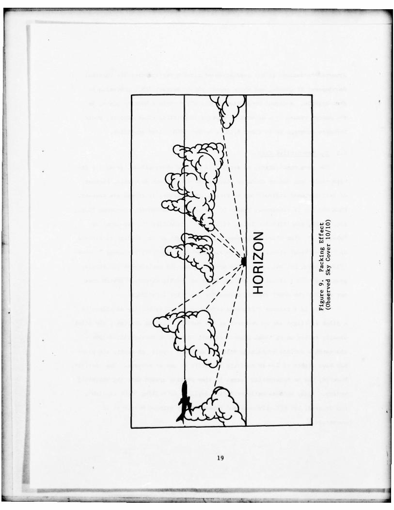
The major reason for the difference between objective and subjective
cloud amounts is the “packing effect” noted in Figure 9. The observer is
18
- ~~~~~~~~~~~~~~~~~~~~~~~~~~~~~~~~~~~~ - - - ~~~~~~~~~~~~~~~~~~~~~~~~~~~~~~~~~~~ ~~~~~~~~~~~~~~~~~~~~~~~~~~~~~ -~~~~-~~~~~~-• --,.
~~~~ -• • _ ----•~ -- _ -~~~
_____ _ ---~~~~~~~~~~--
‘~c cS’~\\
‘i z pN~ ~ 0 00~~
‘•~Sc__
~~ ,“~ cr\i,’,’~~~~ 0,, / I/ I 1 . 4 1I
I 00 .0/ I r40
i~~~~~~~~~~~III/
19

- ~ - ~~~ - narr~~~~— - ________________________________________
directed to include in his evaluation of cloud cover the visibile vertical
development of clouds, and would report 10/10 overcast (OVC) condition in
that example. A direct projection of the clouds onto a horizon plane, in
the manner viewed by a network of vertically pointing cloud sensors, would
indicate coverage to be about 8/10, a broken (BKN) cloud condition.
5.2 The Obscuration Case
The term obscuration, as applied to weather observations, generally in-
fers conditions during which an observer at the surface is unable, because
of surface—based obstructions to vision, to determine if clouds are present.
When the sk> is completely hidden by surface—based obscuring phenomena (e.g.,
fog, smoke, precipitation forms, etc.) FMH—l classifies the sky cover as
“obscured .” When obscured is reported , the height of the ceiling is defined
as “the vertical visibility in the surface—based obscuring phenomena.” When
1/10 or more, but not all, of the sky is hidden (by surface—based obscuring
phenomena) FHII—l classifies the sky cover as “partly obscured” (which does
not satisfy the FMII— l specifications for reporting a ceiling).
There is a radical difference between vertical visibility as viewed by
• a pilot in flight and an observer at the surface. During daylight , the pilot
usually relies on an ideal general target: a massive terrestrial object —
the earth’s surface containing multiple contrast points; at night , the pilot
m a y have lights of low to moderate intensity to use as targets. The observer,
however, has no contrasting target to view peering upward into the obscuring
medium. Aids, such as balloons during daylight or ceiling light at night ,
can be used, but effectiveness and repeatability between observers is
uncertain.
20
_ _ _ _ _ _ _ _ _ -

- -~ • _-
We know of no instrument capable of quantitatively measuring the extent
of partial obscuration, total obscuration or vertical visibility. Yet,
de8pite the weaknesses in objective or subjective methods of making such ob—
servations, FMH—l defines a ceiling in part as “the vertical visibility in
• a surface—based obscuring phenomena.” Because of this FM}I—l specification ,
we’ve devised a technique to give an inferred partial obscuration or verti-
cal visibility observation using a combination of cloud measurements, hori-
zontal visibility and air temperature. This subprogram in our algorithms
is based on a review of some huma n observations in obscuration conditions,
but there has been insufficient data to fully test it. In an extreme case,
virtually no clouds within ceilometer range for the latter portion of the
sampling period and visibility below about 1 1/2 miles , the algorithm can
indicate a total obscuration.
The obscuration case is the weakest element in the automated cloud ob-
servation . The method , perhaps , can be revised to reduce some inadequacies.
But there’ll not be a truly objective observation of this phenomena until
an appropriate sensor is available .
Two subprograms are described in the Appendices. One generates partial
obscuration and assumes .2 of the sky is obscured . The other produces
• several levels of vertical visibility into a total obscuration.
The success of automating cloud observations is not strictly contingent
upon duplicating the human observation . Although reliable, the exact repeat—
ability and precision of human observations has yet to be determined. While ‘
there are some d i f ferences in basic techniques, in a comparison between
automated and human observations, neither is “more correct.” Instead, both
are similar means of describing physical conditions for which there is, as
• yet , no ground truth.21
~ - —; ~~~~~~~~~~~~~~
6. CLOUD INSTRUMENTATION
The RBC was used for data acquisition in these tests. Their sheer
bulk, long baselines and hearty installations made changes in network con—
figuration impractical. Still other problems with this sensor (not designed
for automation) dictate little future for it in operational AV—AWOS networks.
Sensor performance was adequate in our test mode.
6.1 Rotating Beam Ceilometer
The standard RBC is the most widely used cloud height indicator (CHI)
today. This instrument consists of a rotating projector and a vertically
pointing detector. The baseline is usually 400, 800 or 1200 feet: we use
800 feet. The standard RBC projector sweeps the detector ’s verticam beam of
receptivity once every 6 seconds, wIth the measuring scan (0° to 90°) requir—
ing 3 seconds. Its efficient height range is nominally up to 10 times the
baseline. Because of pragmatic sensor and trigonometric limitations, cloud
heights in our tests were limited to measurements below 7000 feet.
For our experiments, several modifications were made to the standard
RBC. An optical zero switch was added to reduce alignment errors, thus
giving greater accuracy at higher cloud heights. An electronic circuit was
designed to allow only one projector lamp to be used , thereby reducing the
measurement cycle to once every 12 seconds. This sampling interval was more
than ample for our data collection needs since the AV—AWOS algorithm used
just two scans per minute. The output of the RBC, normally analog, was
routed through a digitizing system to detect peak amplitude signals, which
indicated the presence of cloud bases.
22
L~ ~~~~~~~~~~~~~~~~~~~~ - - —--
~~~~ .~~~ — •J~~ - — —~~~~ .--- ‘-.~~•-- — - — —

• -.
___________
6,2 Network Spacing
The design length of each leg of the ceilometer triangle was about 7
miles. Assuming the observer can see only to within 8° of the horizon when
cloud bases are at 3000 feet, the observer’s diameter of view is about 8
miles.
The number of CHI ’s to use represents a difficult choice. Although an
infinite number of sensors in the network area would provide near perfect
sampling, that approach was impractical. However, one CIII was ]ocated at
each vertex of the network triangle. The decision was based on economic
considerations and the availability of sensors. We were also influenced
by the work done by Duda, et al., (1971).
7. CLOUD PROCESSING STRATEC,Y
Processing strategies for producing an automated cloud observation must
consider the temporal and spatial variability of cloud elements, and the
characteristics and sampling volume of the sensor in use. In subsequent
paragraphs, we assess these factors to develop a technique that is sensor
independent. While sensor independent, the technique assumes the use of a
vertically pointing cloud height indicator (e.g., RBC, laser ceilometer,
fixed—beam ceilometer).
7.1 Clusterinl
Clustering is first done independently for each network RBC. The
AV—AWOS computer maintains a 30—minute running file of cloud heights re-
ported at each site. At designated intervals, the program clusters these
stored heights into layers and determines the height of each individual
layer. This clustering procedure enables us to mathematical ly combine dif-
fering cloud height measurements into representative levels.
23
~
— • - - -~~-~~ I ~~~~~~~~~~~~~~~~~~~~~ - • -
-: - -— -- --- --~ - ~~~—~~—
~~~~~~~~~~~~~~~ —
~~~— ----• —--
~~- _
~~~~~~~~~~~ .
The method we use is “hierarchical clustering” as described by Duda,
et al., (1971). In this technique, we initially consider our (n) cloud
height measurements (from 30 minutes of data) to be a set of a clusters
which we order in increasing height (h) so that h1 ~ h~ ~ h3 ~ hn. The
• step from n to n—i clusters is made by computing a least square distance
between adjacent clusters and then merging the closest pair . The iteration
process continues and could conceivably end with all data in one final
cluster. Figure 10 is an example of the hierarchical clustering procedure
for each ceilometer. in this example, we started with a total of nine
clusters, each a single cloud height arranged in ascending order .
In our technique, clustering stops at five cloud layers. We then
determine if there should be any additional combining of these layers using
various meteorological considerations, such as the distance between adja-
cent cloud layers. In our tests at Dulles International Airport , Chantilly,
Virginia, (LAD), we found this combination of techniques saved computer proc-
essing time and yielded number of layers and layer separations more repre-
sentative of human observations.
Figure 11 illustrates the clustering technique applied to cloud heights
from an RBC site 7 miles NE of Patrick Henry International Airport , Newport
News, Virginia,(PHF). We plotted the lowest cloud height reported each min-
ute from that site. At the beginning of the data period , the cloud heights
grouped naturally into layers — one about 1500 feet and the other at 3500
feet. Near the end of the period , the upper layer lowered to 3000 feet
while the lower layer became less evident. Using only the data set from
this particular RBC, the automated observation would be:
24
-
~
-- • - --~ —-—•-~~~ - -
-T~~~~~~
-:~~~~ ~~~~~~~~-

-- --~~~- - - - -~~~~~~~~~~~~--— - -- - - - -
1
~~
0
- :: ::~~~: :: ~~~~~~~~~~~~~~~~~:: :.~: I
~h ~~ ~~ o
0 01-~ 0C., ~
C., ~3z
25
_ _ _ _ _ _ _ _ _ _ _ _ _ _ _ _ _ _ _ _ _ _ _ _ _ _ _ _ _ _ _ _ ~~~~~~~~~~~~~~~~~~~~~~~~~~~~ ~~~~~~~~~~~~~~~~~~ -• •_— ~~• -_ - - ~ - - - ‘.— ...a ---

— - - —• -- - - .: ~~~~~~~~-~~
-_ ~~~~~~~~~~~~~~~~~~~~~~~~~~~~~~~~~~~~~~~~~~~~ ~~~~~~—•-•
~~—-———- - — — - - — - -~~~~- — --- • --- - -
—I’
K K N
1’xJc
xK —
• xK
KK
K KK
K —K
KK
KK
KK
X a’K 0
K 0K
K ~~~~~~~~
I’— ~KK
N Z*
K — -‘-4K ~~~ ~ -~~~ I-xx L
K ‘-/ <
~K K LI ~~~~~
‘Kx
K *— 4_J~~_
K*
x x• K I
KK
K I ’-4K T
K
KK
K
K 4~1
K .cnK K —
K — Qx
K 1.Nxx
xK
K*
KX
~~ ~~~~~~~~~~~~ ~~
C 14 E-aNH ) ..LH9 I JH ‘CnD~~D
26
L_ . ~~~~~~~~— ‘
~-~ —~~~ ~~~~~~~~~~~~~~~~~~~~~~~~~~~~~~~~~~ ~~~~~~~~~ -

r - - ~~~~~~~~~~~~~~~~ _ _
Time Observation
30 minutes 15 SCT M37 OVC60 minutes 16 SCT M36 BKN90 minutes M30 BKN 35 OVC
The layers, as determined from each of the three ceilometer sites, are then
merged into a common pool and tested again to see if they can be (meteorologi—
cally) combined. The algorithm then selects the most significant layers (up
to 3) based upon cloud information (height and amount) and outputs these
layers as the automated cloud observation. The precedence for significant
layers begins with the lowest scattered (SCT) layer, followed by the lowest
BKN layer and then various combinations of layer types and heights. The
AV—AWOS computer maintains a history of the cloud hits from each ceilometer
site. These data are used to compute and format remarks such as “d c LWR NE”
or CIG 20V26.”
Except for one step, the single ceilometer algorithm processes data in
virtually the same manner as the three ceilometer algorithm. When a single
ceilometer is used, double weight is given to the last 10 minutes of the
30—minute sample. Since the overall sample and sampling area is smaller,
we’ve added this recency weighing for the determination of cloud layers.
Directional cloud variation remarks are not generated.
7.2 Determination of Cloud Mount
Cloud amount is determined by dividing the number of hits in each layer
by the total possible hits (60) during the 30—minute sampling period. For
the lowest layer, the ratio of the hits to the total possible hits in that
layer only determines whether that layer is classified as SCT, BKN or OVC.
Surmuation totals of all hits, up to and including that level, are used to
classify the higher layers .
27
- -~~-—-----—--- - - — -—- •— - ~~ - -- ~~ - -~~~ —~-~~~~~~
- _—_-~~~~~
In our algorithms we use observed population proportions of .05, .55,
and .87 as break points for SCT , BKN and OVC w i t h a samp le size of 60 inde-
pendent measurements. In this manner , we can be ‘)0” confident tha t our ob-
served proportions are within ±.l of the population proportions.
7.3 Determination of Sky Conditions 1)uring Obscuration
The cloud algorithm was designed to separately treat those cases in
which all or part of the sky is hidden by surface—based obscuring phenomena.
This is typical in the case of fog , and occas iona l ly true for 1 recipitation ,
particularly snow. The algorithm reports a partial obscuration when cloud
layers are detected and visibility is below a b ou t 1 1/2 miles: an arbitrary
0.2 cloud amount is added to the sur ~mat ion t o t a l and —x p l a c t ~ h~~f o i - ~ the
f i r s t layer . To satisf y the requ i reracnt t h a t v e r t i ca l v i s il ’i f lt ’ ; be de te r -
mined when the sky is c o m p l e t e ly h i d d e n b y a ~ i 1 ac e — b i s e d ob s c u r a t i o n , ~ e ’ve
formulated this procedure — when lo~;~ t i i ~n t i v t ~ c l o u d m o a su r en en t s are re-
corded in the last 10 mInu tes o the s • iin p l in g ~~~~~~~~~~ and v i s i b i l i t y is below
about 1 1/2 miles , the obscur • i t i on s a l - p t o~’ t a m i s .~ 1 e~ u p . TLe s t ih :~rogr arn
overrides the repor t f r o m t h e c 1 o n ~~i a i~~~r 1th :’n • t n l ou t ~‘I t t s ~AX ’ as t he ind i-
cation of to ta l obscu ra t ion . “A r e p r e s e n t s v e r t i~ ii visi b ility. Selection
of a value is based on consideration~ such as v I s l h l l i ’v and •- , i r t4 r lpo r ature.
Compar isons of human vs • t a I m i 1 t~~~ ‘so r v i t i o ns ha ’~~- ~t i t - n r~m dv using
this procedure . The technique has ,•en improvised so le ly t o s.st ist v the re-
quirements for determination of vertical visibilit y and extent of obscuration.
It is the weakest of the AV—AW OS m e t h o d s .
8. FIELD TESTS
Fully automated weathe r observations were used in an o p e r a t ion a l t e s t
at PHF during the period January 6 — ~~, i v ~~ 1q78. .\ l g o r i r l : r n s had been
2M
•~~~~ - --~~~~~~ -~~~~~—~~~~

developed based on data acquired from an earlier test program at tAD from
mid—1976 through early 1977.
In these tests , the automated observations were compared with routine
observations made by the duty observers. Although the observers were dedi-
cated and diligent , their time was shared with other , sometimes more insis-
tent , demands. The PHF point of observation did not facilitate visibility
observations. Visibility markers were few and not evenly distributed about
the horizon. To those reading this report who are familiar with the vicis-
situdes of weather observing, more need not be written.
8.1 Results of Automated Cloud Observation Tests
An automated sky condition observation was generated each minute, but
we limited our test data set to the number of “record” hourly (human) ob-
servations available. This set was further limited to periods during which
the hu man observer reported clouds on several consecutive observations. The
final data set totaled over 600 observations. Some comparisons are made with
earlier results obtained on our network at tAD (Bradley et al., 1978).
In the following comparisons, “AV—AWOS” means that the data is derived
from our three sensor CIII network and processed by the AV—AWOS cloud algo-
rithms. “Two separated RBC ’s” means that the data from two RBC’s in our
network are processed separately as if each was a complete and independent
three sensor CHI network.
Table 1 shows a comparison of cloud layers reported by various methods;
the number of cloud layers reported for each observation was put into one
of four categories (0, 1, 2, 3 layers). The number of observations in each
category was then computed for ordered pairs of observations obtained by
several different methods (e.g., human vs. AV—AWOS algorithm) and a 4x4
29
~~~—~~~-.- ---

- ~~---
~~ —- - -~~~~~~~~ r~~~~ --
matrix formed for each pai r. Agreement to ± I layer means, for example,
that a human report of 1 layer would be compared with the number of observa-
tions in the 0, 1, and 2 layer categories of the appropriate paired sensor.
TABLE 1
NUMBER OF CLOUD LAYERS: COHPARISON OF METHODS
Methods % Agreement ± 1 Layer
AV—AWOS/IAI) Observer 74%AV—AWOS/PHF Observer 87%Two Separated RBC’s—IAD 89%Two Separated RBC’s—PHF 92%AV—AWOS/Separated RBC—PHF 85%
Table 1 tests our hierarchical clustering techniques. The general
I’ agreement among methods indicates that we are indeed clustering data derived
from various sources in a consistent manner. The strong agreement between
the AV—AWOS/PMF observer comparisons (87%) indIcates that the clustering
technique is consistent ; and the clusters themselves are similar to those
reported by the human observer. The lower level of agreement for AV—AWOS/
LAD observer reflects earlier problems when spurious layers were generated
by RBC system noise. The program was later modified to reject that type
of false RBC measurement.
In Table 2, joint reports of ceilings occurred in upwards of about 78%
of the cases regardless of the method used. The agreement between “two sepa-
rated RBC’s—PRF” (78%) would likely be higher in a fully operational network,
since in this category we suffered the loss of some data in line transmis—
sions across our test network. As with the cloud layer comparisons, the
agreements between AV—AWOS and the PHF observer indicate that the methods
are consistent and in general agreement with human results.
30
— - ~~~~~~~~ ~ •- —

TABLE 2
OCCURRENCE OF CEILING REPORTS: COMPARISON OF METHODS
Methods Z of Joint Occurrence*
AV—AWOS/IAD Observer 78%AV—AWOS/PHF Observer 82%Two Separated RBC ’s—IAD 8lZTwo Separated RBC’s—PHP 78%AV—AWOS/Separated RBC’s—PHF 86%
*Occurrence — either method reports ceiling.
Table 3 summarizes results of ceiling height comparisons. Agreement
between methods is better at the lover, more critical cloud heights but
falls off at greater heights. This is probably due to the characteristics
of the RBC (small errors at low altitude tend to increase with height).
Many of the cases in which the differences were greater than 200 feet
occurred either during nighttime or precipitation periods. This was
particularly the case at PUP where testing was conducted in an operational
mode. Tests at tAD were developmental.
We believe the cloud height and sky cover algorithm to be complete.
This excludes partial and total obscuration for which the algorithm is
inferred rather than empirical. Given a more reliable sensor, less prone to
height and cormnunication error than an RBC, the scores in Tables 1, 2, and
3 would be still higher.
8.2 Results of Automated Visibility Observation Tests
FM observers at PUF took routine visibility observations at ground
level. When visibility dropped below 4 miles , observations were also taken
at the airport control tower level of 45 feet , a standard procedure. In
31
-
~
- ,-‘ ~~~~~~~ - ~~~~~~~~~~~~~~~~~~~~~~~~~~~~~~~~~~~~~~~~~~~~~~~~~~~~~~~~~~~~~~~~~~~~ . -

TABLE 3
CEILING HEIGHT VALU ES: COMPARISON OF METHOD S
1. Ceiling : 100 to 1000 feet
Methods Z Agreement to ± 200 feet
AV—AWOS/IAD Observer 96%AV—AWOS/PHF Observer 75%Two Separated REC’ s—IAD 82%Two Separated RBC’s—PHF 85%AV—AWOS/Separated RBC—PHF 92%
2. Ceiling: 1100 to 3000 feet
Methods % Agreement to ± 400 feet
AV—AWOS/LAD Observer 63%AV—AWOS/PHF Observer 53%Two Separated RBC’s—IAD 82%Two Separated RBC’ s—PHF 75%AV—A~~S/Separated RBC—P1IF 74%
32
- --- - --
~
---- ~~~~~~~~~~~~~~~~~ ~~!~~2 ~~~~~~~~~~~~~~~~~~ ----- —-- A. ~~~ -~~- — -~~~--~~~ -:~._r

— -
both cases, distribution of visibility targets was limited by circumstance.
The only adequate visibility marker for visibilities greater than 2 miles
was a 500—foot smokestack 7 miles to the north of the observer. In our
analyses , we used only the viBibility reported by the ground observer.
Our three ‘.ideographs were sited to avoid local sources of moisture
and fog. However, local sources of pollution, particularly automotive
emissions, appears to have affected one of the sites. Two of the Videographs
were located on low roofs while the third was at ground level.
For the following comparisons, both sensor and human visibility values
were first rounded to the nearest mile. The number of visibility observa-
tions in each of nine categories (0, 1 . , 7, 7+) was then computed for
pairs of observations obtained by different methods (e.g., sensor vs. sen-
sor , human vs. sensor), and a 9x9 matrix formed for each pair. Tables 4 and
5 were prepared from these matrices. In these tables , agreement to ± 1
mile means, for example, that a visibility category of 3 miles for a method
based on human PV would be compared with observations in the 2, 3 and 4
mile range categories of the appropriate paired sensor. While a sensor PV
was generated each minute (1440 per day) , our data set was limited to the
number of “record” human observations available (24 per day). We further
limited this set to those days on which the human reported an obstruction
to visibility. The final data set totaled 490 observations.
Table 4 shows the results of compar isons between totally objective
sensor derived visibility observations . First , sensor observations from
two of the three Videograph sites were compared with each other and level
of agreement recorded. Then a sensor PV observation derived from the three
sensor network was compared with a similar observation from one arbitrari ly
chosen network sensor .33
J

- - -~ ~~~~~~~~~~~~~~~~~~~~~~~~~~~~~~~~~~~~~~~~~~~~~~~~~~~~~~~~~~~~~~~~~~~~~~~~~~~~~~~~~~~~~~~~~~~~~~~~~~~ ~~~~~~~~
TABLE 4
VISIBILITY OBSERVATIONS: SENSOR vs. SENSOR
Methods Agreement + 1 Mile
1. All Visibility Values:
2 Separated Sensors—PHF 87%2 Separated Sensors—lAD 89%Sensor PV/Single Sensor—PUF 92%
2. Sensor Visibility Below 5 Miles:
2 Separated Sensors—PHF 90%2 Separated Sensors—lAD 90%Sensor PV/Single Sensor—PUF 93%
Results demonstrate consistently high and stable relationships between
objective visibilities derived from individual sensors in the visibility
network. The experiment was conducted at both lAD and P1W with almost
identical ef f ec t .
The results in Table 4 show the intercomparisons of sensor derived objec—
tive visibility observations, are not duplicated when human subjective ob—
.ervations are introduced. Table 5 shows comparisons of objectively and
subjectively derived visibility observations. Greatest agreement occurs
when the observer records visibility below 5 miles. But strength of com-
parisons weakens for the other examples.
In another visibility test,a single visibility sensor was located at
PH? on a roof about 35 feet directly above the normal FSS point of observa—
tion . Figure 12 shows the spatial relationships between this site and the
three remote network sites. Visibility was derived by averaging 10
34
~~~~~~~~~~~~~~~~~~~~~~~~ --~~~~~~~~~~--- -•—-—~~~~~~~ ~~~~~~~ --~~~~~-- - - -
~~~~~--
~~~~~~~~ - -

TABLE 5
VISIBILITY OBSERVATIONS : HUMAN vs. SENSOR
Methods Agreement ± 1 Mile
1. All Visibility Values:
Sensor PV/PRF Observer 697.
Sensor PV/LAD Observer 58%
2. Observer Visibility Below 5 Miles
Sensor PVIPRF Observer 80%Sensor PV/ IAD Observer 72%
3. Sensor Visibility Below 5 Miles
Sensor PV/PHF Observer 57%
Sensor PV/IAD Observer 45%
35
- —-~~~~~- - -
~~~~~ - — - - — - - - - ~~~~~
--
- _ _ _ _ _ _
- -_4-~w~_______ __ _ - ~~~~ — ~

P. - — -- —--- --- -~~ — - -
- - - -
-
-
I E Fss
Site I ~~~~~~~~~~ ‘S
.
‘~~
-
,~
“ It
~~~~~~~~~~~~~~~~~~
‘S
Si te 3
Site 1 — Denbigh — West site. Near a heavi ly t ravel led t r a f f i cin te r sec t ion ; on a roof w i t h p ro jec tor and de tec to rabout 30 ft. above ground .
Site 2 — Kentucky Farms — Northeast site , pointing toward an openfield. Elevation about 10 ft. above ground .
Site 3 — Hampton Roads Academy — Southeast site. About 1.2 mileswest of a city trash incinerator smokestack. About 20 ft.above ground pointing over a soccer field.
Figure 12. Visibility Site Locations at Newport News
36

once—per—minute Videograph output values and converting this value to vlsi—
bility based on day or night conversion equations. Results were also sepa-
rated on the basis of whether precipitation was occurring.
Table 6 shows the results of intercomparisons between the roof Video—
graph and AV—AWOS sites. Best agreement is between the roof Videograph and
human observer during the day.
Psychophysical and other limitations are often associated with subjec-
tive observations. The influence of human factors is discussed in detail by
Lefkowitz (1966) for another type of objective visibility observation (RVR).
Human limitations include, but are not limited to, visual illuminance thres-
hold , visual contrast threshold , dark adaption, availability of appropriate
visibility targets, and pressure of other duties.
There appears to be the effect of a “non—linear” human/backscatter sen-
sor relationship. We noted strong relationships between human and Videograph
der ived visibil i ty in the presence of hydrometeors (e.g., rain, drizzle,
snow). When lithometeors (e.g., haze, smoke, dust) reduced visibility,
the visibility algorithm (using Videograph measurements as input) character-
istically produced lower visibilities than those reported by the human ob-
server (Table 7). Although we believe the visibility algorithm performance
to be effective, performance of the Videograph needs review.
9. SENSOR NETWORK CONFI GITRATI ON
The earliest elements considered in the AV—AWOS work were sensor network
size and number of cloud and visibility sensors. Some guidance was available
from a study funded by the FAA (Duda et al., 1971) . The study, using several
assumptions, indicated that three cloud sensors could be used to produce
cloud observations comparable to those made by humans.
37
- -~~~~~~~~~- - ---------- - --- - - - — — • - ~~~~~~~~~~~~~~~~~~~~~~~~~~~~~~~~~~~~~~~~~~~~~~~~~~~~~~~~~~~~~~~ - -

— - - - r’-r - - ~~~~~~~~~~~~~~~~~~~~~~~~~~~~~~~~~~~~ -‘--‘--- - - .—~—- - - -
TABLE 6
VI SIBILITY COMPARISONS BETWEEN VAR IOUS REPORTING SYSTEMS
A. % Agreement Between Roof Videograph and Simultaneous Observation Within
± l M i l e
All Precip No Precip Precip No PrecipCases Day Day Night Night
Human 67% 74% 75% 60% 63%AV—AWOS 69% 68% 70% 80% 65%Site 1 70% 72% 73% 73% 66%Site 2 68% 65% 77% 78% 60%Site 3 61% 70% 69% 68% 517.
B. 7. Roof Videograph > Simultaneous Observation Outside of ± 1/2 Mile
All Precip No Precip Precip No PrecipCases Day Day Night Night
Human 35% 48% 32% - 47% 32%AV—AWOS 53% 49% 49% 50% 57%Site 1 49% 49% 42% 48% 54%Site 2 537. 48% 41% 54% 63%Site 3 65% 50% 53% 61% 77%
C. % Roof Videograph < Simultaneous Observation Outside of ± 1/2 Mile
All Precip No Precip Precip No PrecipCases Day -
Day Night Night
Human 34% 16% 25% 32% 44%AV—AWOS 7% 11% 7% 7% 7%Site 1 117. 20% 14% 14% 7%Site 2 10% 16% 11% 12% 6%Site 3 7% 12% 9% 11% 3%
38
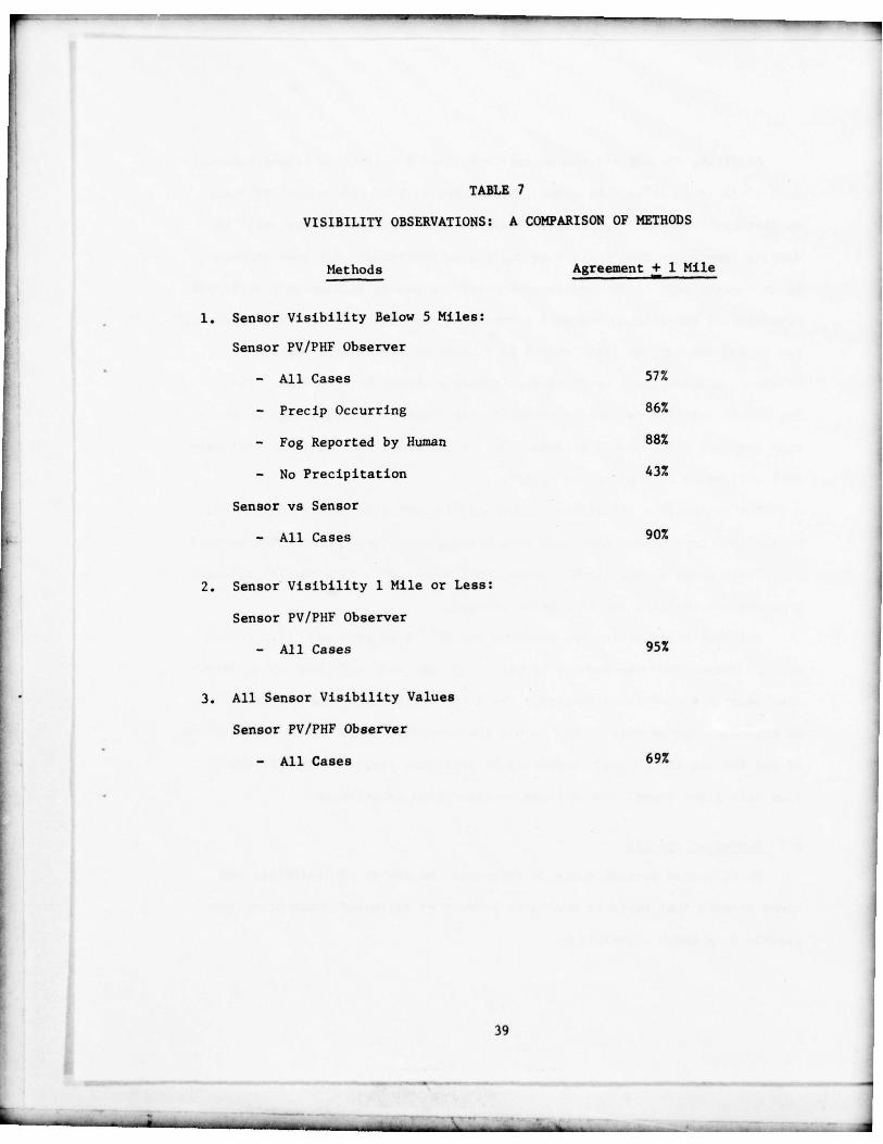
TABLE 7
VISIBILITY OBSERVAT IONS: A COMPARISON OF METHODS
Methods Agreement + 1 Mile
1. Sensor Visibility Below 5 Miles:
Sensor PV/PHF Observer
— All Cases 57%
— Precip Occurring 86%
— Fog Reported by Human 88%
— No Precipitation 43%
Sensor vs Sensor
— All Cases 90%
2. Sensor Visibility 1 Mile or Less:
Sensor PV/PH F Observer
— All Cases 95%
3. All Sensor Visibility Values
Sensor PV/PHF Observer
— All Cases 69%
39
- ~~~~~~~~~~~~~~~~~~~~~~~~~~~~~~~~ - - -
~~~~~~~~~~~~~~~~~~~~~~~~~~~~
-- - — .— —.-- -— -—------
~~------ —.-.
~~~~~--- .
~~~~~ -———— — — -- - - ---- - - - ---------- - --
At first, the NWS program manager specified a ceilometer triangle having
legs of 12 to 15 miles. He wrote, “My concern is that operational aviation ,
as distinguished from the ‘flight standards ’ and ‘safety ’ matters , will be
wanting assurances that our system won ’t give pessimistic information when
it is clearly safe to descend through breaks in clouds within the operational
proximity of the airport and make a normal visual flight rules (VFR) approach.”
Due to FAA concern, he later agreed to a triangle with 8 mile legs. He
believed , however, that no fixed—size triangle should be specified . That
is , should mult iple sensors be required , the shortest t r iangle legs at which
data remained valid should be selected . He believed , at that time , that net-
work size would be a sensitive factor.
The choice of a visibility network configuration followed . Since visi—
bi l i ty is a less stable phenomena than clouds , we decided to keep the sensors
relat ively close to the a i rpor t operat ional area , and used a smaller t r iangle
than the one used for the ceilometer network.
Ori ginal plans called for portable v i s ib i l i ty sensors and l idar ceilom—
eters. Sensor networks were to be varied in size and conf igura t ion to deter-
mine sensitivity of those factors. The lidar ceilometers were not delivered
as expected , and we were forced to use the non—portable RBC . The fixed nature
of the RBC and the general d i f f i c u l t y of obtaining sensor sites with quali-
fied data lines doomed the variable configuration experiments.
9.1 Number of Sensors
We conducted several tests to determine the number of visibility and
cloud sensors that would be needed to produce an automated observation corn—
parable to a human observation ,
40
L - ____________________________________________________ - -

— — —-
a. Visibility
In our first visibility test , we located three backscatter visi-
bility sensors next to each other at SR&DC and processed each output sepa-
rately through AV—AWOS visibility algorithm. For 158 independent samples,
the correlation coefficient between the sensors exceeded .98. We then
placed the sensors at the vertices of our visibility network around lAD
(Figure 1). For 103 independent samples taken during June—July 1976 with
the sensors spread 3 to 4 miles apart , the correlation coefficient between
the sensor at SR&DC and the individual sensors at the other sites ranged
from .79 to .96. Denoting the sensor at SR&DC as our standard , we then corn--
pared differences in visibility between each remote site and our standard .
The worst case situation of the two data sets is shown in Table 8. Even in
this case , the d i f f e r ences between v is ib i l i t ies from our standard and rom
our remote sites were ± 1/2 mile or less on 86% of the observations.
Table 9 shows a similar plot for PHF data. In this set, visibility
data from two separated sites were compared every one—half hour for May
4—6 , 1978. While there is some bias towards higher visibility at sensor 2,
the spread in the data shows most of the comparisons grouped with ± 1/2
mile of some central value.
At PH? we located the three Videographs at sites selected to be clime—
tolog ically fav orable for de tecting the onse t of lower visibility during
varying synoptic weather conditions. We then examined two 30—day data
periods (720 observations each) : one for the winter season , another for the
spring season. Using the SEV from each of the three Videograph sites, a
“remark” (supplemental comment required by FMH—l) was generated if a sensor
visibility differed from the PV by more than 1/2 mile. The results are
41
—-- - - ---— - - - — —- —“ - --- - - ----~
--- ___.;~~~ _ _~~~~_ _ _ _ ______ ~__ _ _ ——— --—— -

- ~~ - ~~-~~~~~~~~~~~~~~~~~~~~~ ‘ —~~~~ -- --- --- -- —~~~~~~~~- - -~~~~
TABLE 8
Visibiliti es at Site 2 (lAD Network)Compared With V isihilit ie s at Site 1 as Standard
D I F F E R E N C E IN V I S I B I L I T Y ( M i l e s )(SENSOR 1 — SENSOR 2)
—3 —2 — l — 1/2 — 1/4 +1/4+1/2 +1 +2
0— 1/2 2
1/2—1>..
~~~~~~~~~~~ 1-2 2 13 19 1L~ ~)I-~
C) — — — — — — —~~~~~ 2—3 1 1 5 10 3
~~~~ 3—4 1 2 4 5 4 1
4-5 2 1 2 1
— u 5—6 1 1Ci)
6-7 1
7 2
42
— - - -~~~~~~~~~~~~~ ~~~~~~~~~~~~~~~~~~~ ~~~~— - --
~~~~~~~~~~~-~~~~ -- - -— —~~~ - ‘ - - - .~~~~~~~~— --

-- r~~~ -----———-~~~~~~~~~ ~~~~~~~~~~~~~~~~~~~~~~~~~~~~~~~~~~~~~~~~~~
TABLE 9
Visibilities at Site 2 (PHF Network) ComparedWith Visibilities at Site 1 as Standard , May 4—6, 1978
D I F F E R E N C E IN V I S I B I L I T Y ( M i l e s )(SENSOR 1 — SENSOR 2)
—3 —2 — l — 1/2 —1/4 ±0 +1/4 +1/2 +1 +2 +3 +4
0—1/2
1/2—1
a — ’ 1-2 3 1 1 2 1 4 1i— C) —
2-3 1 1 ô 6 4 4— — —
3—4 1 1 1 1 4 7 3—
4—5 1 2 1 4 6 7
5-6 2 4 4 1
6-7
7 1 1 4
43
_ _ _ _ _ _

- - - ~~~~~~~~~~~~~~~~~~~~~~~~~~~~~~~
summarized in Figure 13. The distribution of remarks can better be ex-
plained by local variations in ground fog and urban pollution than by any
variation in the synoptic scale elements. As an example, the ten cases of
lower visibility at the west (Denbigh) site in the winter period were due
to enhanced backscatter due to smog pollution on mornings with temperatures
near or below freezing. The absence of low visibility remarks at Denbigh in
the spring season was due to the presence of ground fog at the other two
sites—sites situated in less developed areas.
The question of how many visibility sensors are needed in an automated
system should be based on the nature of the visibi l i ty observations needed
at the observation site. As stated earlier, FMI~—l defines prevailing (human)
visibility as, “The greatest visibility equaled or exceeded throughout at
least half of the horizon circle which need not necessarily be continuous.”
The only off—the—shelf visibility sensors now available have very limited
volume sampling areas. Therefore, it appears that one sensor will not
satisfy the FMH—l definition of prevailing visibility. Three sensors , then,
appear to be the minimum needed for prevailing visibility. If a lesser form
of visibility is acceptable , e.g., station visibility (index of visibility),
one sensor will do. In both cases, data would be processed as indicated by
the algorithms in the appendices.
b. Clouds
In the PHF and lAD t ests , two RBC’s, separated by a distance of 8
miles, jointly reported the occurrence of a ceiling in upwards of 78% of
the observations in which either RBC reported a ceiling. With the ceiling
reported at or below 1000 feet, ceiling heights agreed to ± 200 feet in 82%
to 85% of the observations. During two test periods at PHF (Figure 13),
44
~~~~ -~~~
— .1

~~MARK JAN -FEB APR—MAY
VSBY
I
GTR ~~~~~~~~~~~~ 31
1
lO~~~~~~~~~7
28
4~~:c::J
~~~~~~~~~~~~~~~~~~~~~~~~~~~~~~~~~~~~~~~~~~~~~~~~~~~~~~~~~~~~~~~~~~~~~~~~
18 N/A
Figure 13. Distribution of Remarks for Clouds and Visibility
at Each Sensor Site at PHF. Amount is Indi cated at Site.
_ _ - - --

- _ _ . _ _ _ __ _
~~~_ _
~~~~7 _
~~~~__ -—- — ____________________
only a few reports of CIG HIR or CIG LWR remarks were generated . Thus, a
three sensor network appears to offer little additional information over a
one sensor network in most cases.
There are specialized situations, however, where more than one sensor
would be required. For example:
— a zone, in sight of the airfield , where clouds form and
linger.
— rapidly moving stratus shields in a coastal zone.
9.2 Network Spacing
a. Visibility
— We used a nominal 3 mile spacing between visibility sensors. At
that distance our tests showed a good agreement between sensors. As net-
work size increases, we would expect this agreement to decrease; however ,
we do not know the rate of decrease. ThUS , our specification of size is
adequate, but not unique .
Tests at PHF showed a 92” agreement (to ± 1 mile) between sensor PV
and a single sensor averaged visibility. These results and the sensor vs.
sensor results indicate that , as a minimum , the visibility fran a single
sensor represents a universe extending for a radius of approximately 3 miles
about that sensor. The radius of the universe could be greater but the PHF
and tAD tests show that it is probably not smaller.
b. Clouds
The AV—AWOS cloud report at PHF and a cloud observation generated
by a single sensor showed joint occurrence of a ceiling on 86% of the ob-
servations. Ceiling heights agreed to within ± 200 feet on 92°~ of the ob-
servations. Coupled with the results from two separated RBC’s, we conclude
46
__~~~
_ _-i_ __
— -~~~~~~~~ - - - — ~~~~~~~~~~~~~~~~~~~~~~~~ . -~~~~~- --
— -“ -- —~~~--.

— -~~~~~~~~~ -~~
that at 8 miles separation , clouds sampled by one R3C come from the same
universe as clouds sampled by a second separated RBC. The cloud reports
from a single sensor R.BC thus represent a universe extending up to about 8
miles in radius about said sensor. Since the joint agreement is only 80%,
we do not believe this 8 mile radius should be extended. A circle with a
6 mile radius would probably be more representative.
10. SENSOR SITING
Our experiences at tAD and PHF have pointed up the need for preliminary
site surveys before installing sensor networks at airports.
The primary purpose of a detailed site survey would be to identify
unique conditions that might influence judgments on the number of sensors
needed and configuration. For example, if fog or stratus tends to move in
rapidly from a specific sector , sensors would be located in their path to
provide early warning. In such cases, algorithms may have to be modified.
The best source for information on local peculiarities should be experienced
observers at the stations. Climatological record s and local geography
should also be evaluated as part of the site survey.
In some cases, three sensor arrays may be required. In particular, if
prevailing visibility is considered a requirement at a station, a triangular
network will have to be set up. Particular attention should be given to
avoiding highly localized sources of pollution or fog. For example, in the
PHF area, heavy vehicular t r a f f i c near one site occasionally lowered visi-
bility indications from that sector (a more representative sector visibility
could have been obtained by moving that Videograph abou t a quarter mile).
Othe r locations to be avoided are low spots where pockets of fog tend to
form or locations very close to smokestacks. Also, to avoid ground fog
47

— VT’?: — ~~~~~~~~~~~~ - ~~r’rza - — - - - - ________________- -
(< 20 feet deep), sensors should be located 20 to 30 feet above ground.
The exact height is uncertain, since FMH—1 no longer specifies the height
of the visibility observing plane. The 14—foot height the FAA specifies
for the RVR transmissometer may be appropriate.
Other considerations for siting of visibility sensors depend on the
type of sensor used. Specifically , in our tests, we used a backscatter
instrument, the Videograph, which requires about 100 yards of cleared space
in front of it. This meant that open areas such as parks or farmland were
most desirable. When we had to go into developed areas, rooftop sites were
generally the only suitable locations. No matter what sensor is used, the
availability of nearby power and data transmission lines must be assured
before a site is selected.
Siting of cloud height indicators should not be a problem if laser
ceilometers are used. However, requirements to site RBC’s are expensive
and require considerable real estate. If a site survey indicates the need
for a remote site away from the airport , that site must be selected to avoid
localized conditions . For example , at Newport News were forced to locate
an RBC within 1/2 mile of a smokestack. We found that on a few occasions
a smoke layer at that site would cause an indication of scattered clouds
in our PHF cloud report. Although the layer could be seen from the airport,
it did not cover 1/10 of the sky. If single ended laser ceilometers had
been available, the flexibility in site selection would have been greatly
increased . RBC ’s require line—of—site between detector and projector,
underground signal cables , and stable concrete bases for both projector and
detector. If secure government—owned land is not available, it is often
very d i f f icu l t to find private property owners willing to permit such an
installation.48
I - ~~~~~~~~ -

11. FURTHER INVESTIGATIONS
Although we consider the algorithms for objective cloud and visibility
observations to be operational, some weaknesses are present as discussed
earlier in this report. Since there has been no assessment of the pre-
cision and accuracy of subj ective human observations, it’s difficult to
specify standards for automated observations. Therefore, we’re uncertain
as to the “perfection” that can or should be achieved in objective auto-
mated observations. We propose that further investigations, such as those
proposed below, be conducted to resolve uncertainties (they ’ve been limited
to cloud and visibility observation techniques):
— Determine why the Videograph showed lower than human
visibilities during the tests at PHF .
— Seek improvement in the obscuration automation method.
This may include additional sensor input not part of
the original AV—AWOS program.
— “Fine tune” the cloud and visibility observations with
a larger and more certain data sample than thus far
acquired .
— When suitable ceilometers become available , check the
sensitivity of sensor network configurations.
— Investigate variations in data preprocessing that may
be needed for new sensor characteristics,
sampling method , sampling volume and response time.
— Determine how newly—developed sensors (laser weather
identifier , for example) can be used to improve automated
cloud and visibility observation performance.
49
- - - ‘ -~~~~~~~~ - -~~~~~~~~~~ -~~~~~~~~~~ - —
- V T : — ‘~~~~‘
~~~~~~~~~~~~~~~~~~~~~~~~~~~~~~~ -~~~~~ - - - —
— Assess the performance of the AV—AWOS system, thus
far limited to PHF and lAD , to more extreme meteoro-
logical conditions.
— Determine the precision (and accuracy, if feasible)
of human weather observers.
An operational approach to network size and siting should be estab-
lished (as it might be for the construction of a new airport or installa-
tion of an ILS system). These steps, for example, might be followed :
— Form a multidisciplined committee . (Meteorologists,
climatologists , engineers, airport experts , and perhaps ,
members of the user groups) .
— Examine all meteo r olog ical data possible to determine
local weather e f f ec t s , advectio n characterist ics,
direc tional weather characteristics , terrain influence ,
weathe r fea tures that should be inc luded in the ob-
servation , etc.
— Based on the foregoing, legal requirements and the
nature of observation needed , select number of sensors
and design configuration .
— Procure needed property, hardware and software , and
install the system.
— Run the system in a test mode through all seasons of
weather as long as possible before commissioning is
needed . Verify that the system is responsive to require—
ments and local characteristics. If not , correct and retest.
— Commission the system, continue retesting in accordance with
a predetermined program.50
~~~~~~~~~~~~~~~~~~~~~~~ ~~~~~~~~~

‘ “‘ ~z’ ’ r r - — — ‘ A - ~~~~~~~~~~~~~~~ — - —
~~~~
12. SUNMARY
This summary is based on tests and experiences at lAD and PHF. In
addition, we had valuable input from the observers, both National Weather
Service and Federal Aviation Administration , who participated in the
program at PHF .
12.1 Visibility Observations
— The Human Observation: The operational definition of visibility
focuses on the human observer. However, human observations of visi-
bility have many limiting factors. For example, point of observation,
nature and number of visibility markers, and the very curvature of
the earth impart unique characteristics to each observation.
— Sensor Preprocessing: The Videograph, although it has limiting
sampling volume (13 ft.3), samples a relatively large volume compared
to other types of single—ended visibility sensors currently marketed.
Because of this volume,”grab” samples of 2 to 30 per minute show no
significant differences when averaged over a time period of 6 to 10
minutes. A sensor with a faster time constant or smaller sampling
volume than the Videograph will require preprocessing at a greater
rate than two samples per minute.
— Sensor PV: Sensor derived PV (using three visibility sensors) had
only fair agreement with human visibility at tAD and PHF. We believe
this to be related to the limitations of subjective observing tech-
niques , differences between human and automated concepts of observing,
and reactions of the Videograph during certain obstruction to visi—
bility situations. Because of consistency and timeliness, sensor PV
should , in time, replace human visibility as the standards for
observations. 51
_ _ _ _ _ _ _ - -- --j--- -~~~~~ —A

- - -~
— Single Sensor Visibility: The inability of a single sensor to
report sector visibility may be a limitation in some operational
applications. However, our tests showed excellent agreement between
two separated single sensors as well as between sensor PV and single
sensor vis ibi l i ty. Thus , a single sen sor with app ropr ia te p r ocessing
can produce a useful index of v is ibi l i ty . By def in i t ion, a single
sensor could never report PV. It could be used to report “s tat ion”
visibility at smaller or limited—service airfields.
— The Visibility Algorithm: The visibility algorithm for both a
th ree sensor network (PV) and a single sensor (station v is ib i l i ty)
is now at the operational level.
12.2 Cloud OLservatiDn Automation
— Thc Human Observation : The operational def in i tion of sky condition
is aased on the presence of a human observer with inherent limitations.
— Processing Strategy : Test results show that our processing strate-
gies give consistent results and that our computer—generated observa-
tions are in agreement with human observations. Our data sampling,
averaging t imes and network configurations , while not unique , are
appropriate for use in automated surface weather observations.
— Obscurations: Our program for observing total and partial obscura-
tions is marginal. No sensors are currently available that measure
the amount of sky obscured or vertical visibility into an obscuration.
Until such equipment is developed , adequate algorithms for partial
and total obscuration cannot be generated . Our algorithms for obscura-
tions are the weakest part of our program. Under some combinations
of weather conditions, unrepresentative observations of obscuration
can be output by the automated system.
- ~~~~~ ~~~~~~~~~~~ ~~~~~~~~~~~~~~~~~~~ _ __

— Three Sensor Observations : Our cloud algorithm based on a three
sensor CHI network shows good agreement with human observations . Vari-
ances are largely related to differences in human and automated concepts
of observing. Because of its consistency and timeliness , sensor—generated
cloud obse rvat ion should , in t ime , rep lace human observations as the
standard observing p rac t i ce .
— Single Sensor Observations: The inability of a single CHI to report
remarks such as “CIC LWR NW ” may be a limitation in some operationalappl ica t ions . However , our tes ts showed excellent ag reement between
two sepa rated single sensors as well as between network and sing le
sensor observations.
— The Cloud Algor i thms: The cloud algori thms for both a three sensor
(AV—AWOS) network and a sing le sensor application are now at the
ope rat ional level.
12.3 Network Size and Siting
— If prevailing visibility is required , three visibility sensors are
needed — more , if there are unusual local visibility problems .
— Three visibility sensors in normal situations should be installed at
the vertices of an equilateral triangle having approximately 3 mile legs.
The required point of observation should be at the triangle ’s center.
— If an index of visibility is required , one visibility sensor is
needed — more , if the re are local v is ib i l i ty problems .
— In most situations , one ceilometer would be adequate. More would be
needed in situations where directional bias is present .
— If three ceilometers are needed for more representative information ,
they should be instal led at the ver t ices of an equi la tera l t r iangle
53
‘~1
~
~~~~~~~~~~~~~~~~~~~~~~~~~~~~~~~~~~~~~~~~~~~~~~~~~~~~~~

- - - - -
having 6 to 8 m i l e legs. The required point of observation should be
at the t r iangle ’s center .
— We do not believe that the algorithm test results would be affected
by small changes in network configuration.
— Installation of an automated weather system should proceed in a
manner typ ica l of other major avia t ion f ac i l i ti e s . This includes an
i n i t i a l period of invest igat ion to d ef i n e the required ins t rument ne t —
work conf i gura t ion . Continued review a f t e r commissioning w i l l also be
needed .
13. ACKNOWLEDGMENTS
AV—AWOS was developed by the National Weather Service as a joint project
with the Federal Aviation Administration . Engineering and liasion support
were pr ovided by NWS ’s Equipment Development Laboratory : particularl y
Doug las Downen and Wayne H u f f m a n . No t ewor thy among the f i n e suppor t received
from NWS’s Test and Evaluat ion Divis ion were con t r ibu t ions of Paul Chinn ,
George Reeves , W i l l i a m Read , and John Blel loch. The tes ts at PHF were coor-
dinated by Er i c Man del of the FAA . The dedica t ion of the FAA and NWS wea ther
observers d u r i n g the tes ts was exemplary .
14. REFERENCE S
Chishoim , D. A. and Kruse , H . , 1974a: The V a r i a b i l i t y of Visibil ity inthe Hanscom Mesonetwork : A Preliminary Assessment. AFCRL—TR—74—0265Air Force Cambrid ge Research Labora tories , 36 pp.
Chishoim , D. A. and Kruse , H . , 1974h: The V a r i a b i l i t y of A i r f i e l d Visi-bilit y: A Preliminary Assessment. AFCRL—TR—74—0027 Air Force Cam-br id ge Re sear ch Labora tor ies , 32 pp.
Curcio , J. A. and Knes t r i ck , C. L . , 1958: C o r r e l a t i o n between atmo-sp h e r i c t ransmiss ion w i t h b a ck s c a t t e ri ng . J . Op t . Soc. A m e r . , 48 ,686—689 .
54

Duda , R. 0., Manc uso , R. L ., and Paskert , P. F. , 1971 : Anal ysis ofTechniques for Describing the State of the Sky Through Automation ,”Report No. FAA—RD—71—52 , p repared for Depar tme n t of T r a n s p o r t a t i o n ,Washington , D. C., 156 pp.
Calligan , A. M., 1953: Variability of Subjective Cloud Observations —
I, Air Force Surveys in Geophysics No. 33 , Air Force Cambr idgeRe sear ch Cen ter , Cambridge , Massachusetts , 13 pp.
George , D. H. and Lefkowitz , M . , 1972: A New Concept: Sensor EquivalentVisibilit y . Preprints , International Conference on Aerospace andA e r o n a u t i c a l Meteorology , May 2 2 — 2 6 , Was h in g t o n , D. C . , 243—250 .(Avai lable throug h Amer . Meteor. Soc., Boston , Massachusetts).
Hockreiter , F., 1973 : Videograph Calibration . Laboratory Report No.4—7 3 , U. S. Weather Bureau , Test and Evaluation Division , Sterling ,Virginia , 51 pp.
Lefkowi t z , M ., and Schla t te r , R. E . , 1966: An Analys is of Runway V isualRange , Federal Aviation Administration Report No. RD—66-lOO , U. S.Wea ther Bureau , Atlantic City , New Jersey.
NOAA—Nat ional Weather Service , 1970 : Feder al Me teorol og ical Handbo okNo. 1, Sur face Observat ions , U. S. Government Printing O f f i c e ,Washington , D. C., 405 pp.
Sheppard , B., 1977 : Compar ison of Sca tter ing Coefficien t Type Visibil-ity Sensors for Automated Weather Station App lications. Preprints ,International Conference on Aerospace and Aeronautical Meteorology,May 22 — 26 , Washington , D. C . , 201—206 . (Avai lab le through Amer.Meteor. Soc., Boston , Massachusetts).
NOTE: This report is furnished fo r technical informat ion only. The NOAA doesnot app rove , recommend , or endorse any product; and the test and eval-uation results shall not be used in advertising , sales promotion , orto indicate in any manner , either implicitly or explicitly , endorse-men t of the produc t by the National Weather Service.
~~~~~~~~~~~~~ -_ ---

— ~~~~—~~~~~ —— — - S - -~~~~~
--—--- -- - -- -- ,
APPENDIX A
VIS IBILITY ALGORITHM
A-i
- - ~~~ ~~~-—
~~ ~~~~~~~~~~~~~~~~~~~

APPENDIX A
VISIBILITY ALGORITHM
Comments on a Single Sensor Visibility Algorithm
1. The a l g o r i t h m is e s sen t i a l ly the s ingle sensor AV—AWOS a l g o r i t h m used at
PHF and updated by the October ‘78 three sensor a l g o r i t h m .
2. We de s igna t e the sensor o u t p u t as s t a t ion v i s i b i l it y (SV) to d i s t i n g u i s h
it from the prevailing visibilit y (PV) determined by a three station
network .
3. The adequacy of using a single station as opposed to a three station
ne twork must be de te rmined fo r each locat ion by a s i t e c om m i t t e e .
4. A g e n e r a l i z e d f low c h a r t is a t t a c h e d .
Comments on the Three Sensor V i s i b i l i t y A l g o r i t h m
1. The a l g o r i t h m is e s s e n t i a l l y the a l g o r i t h m as c u r r e n t l y programmed in
AV—AWOS and used o p e r a t i o na l ly a t PHF.
2. In Sec t ion l . 4 a , we made p r o v i s i o n f o r p r e p r o c e s s i n g sensor d a t a . Whi le
one grab sample per 30 seconds is adequa te fo r the Videograph , a sensor
w i t h a sho r t e r t i m e constan t might have to be sampled and averaged more
of ten.
3. In l . 4 i , we al lowed fo r c a l i b r a t i o n curves to be i n s e r t e d fo r any sensor .
4. We made a t e c h n i c a l c o r r e c t i o n to Section l . 4 u to b r i n g i t in l i n e w i t h
Section l.4r.
5. Sec t ion l . 4 z is new. This procedure is our method to avoid o s c i l l a t i n g
between two va lues of v i s i b i l i t y . It solves the problem of f:equent
specials because of this oscillation . In one test , 17 o !cillations in
2 hours were reduced to 5.A- 2
- _ - - - - - - - - - - _ -

- - — -— ~~~~- . -
~~~~~~~~~~~~~~—- ~~~—~-———-—
~~~~~~--.— - ---——---— —— - —-—- - - - - — _ — --- - - ________ -
SINGLE SENSOR VISIBILITY ALGORITUM
V1 SAMPLE SENSORFOR 10 M1~1UTES
TSTORE 1
COMPUTE 1 WEIGHTED AVERAGE
SEV OVER 10 MINUTESI.
[~~~~~‘I J STATIO!~1 VISIBILITY
OBSERVAT IO~1 STANDARD AVIATIONFORMAT

____________________ - - ~~~~~~~~~~~~~~~~~~~~~~~~~~~~~~~~ - —~ -~~~~.-—,. ——-—-.———.. - -———--— .--~~-
6. Section l.4ad is new . This procedure prevents more than one v i s i b i l i t y
remark at a time from being outputted on Service A. This procedure is
needed since we saw excessive remarks being generated during our test
- at PHF.
- 7. A generalized flow chart is attached .
A— 4

~~~~~~~~~~~~~~~~~~ ‘ —
.— I—‘-I C)
>-C)C’)
1._i LU C)C) —I —
C) Lt’s I.-C’) - >.
—LU ...J >• C/) >-
I— U)L~i
-
LU ~— LUC.. ) •‘ c~Q_. —
— wUi C/) - I—
C.f) __ Li (I)
I ILU Li
— c~C) =D _ _ _ _
>-I—-J
-4(I)
A-S
- -
~~~~~~~~~~~~~~~~ ~~~~~~~~~~~~~~~~~~~~~~~~~~~~~~~~~~~~~~~~~~ --~~—~~~~-- .-~~~~~~~~. ~~
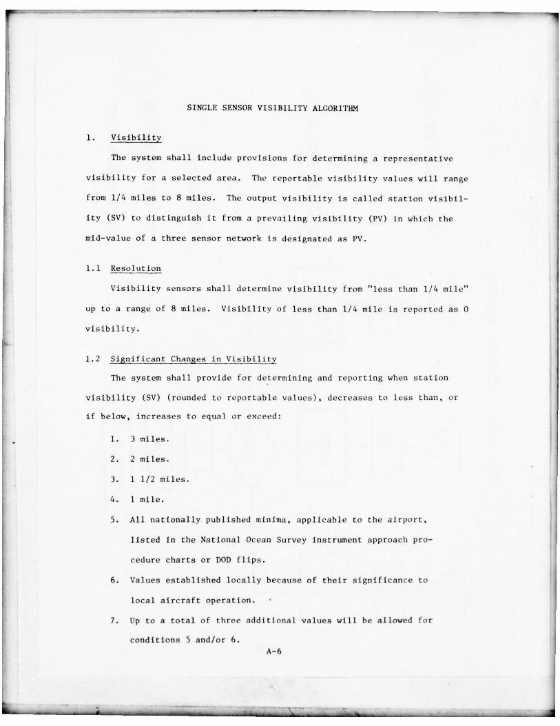
SINGLE SENSOR VISIBILITY ALGORITHM
1. Visibility
The system shall include prov i s ions for de te rmin ing a r epresen ta t ive
v i s i b i l i t y fo r a selected area . The r ep o r t a b l e v i s i b i l i ty values wi l l range
from 1/4 mi les to 8 miles . The o u t p u t v i s ib i l i t y is called s t a t i on v i s i b i l —
i t y (SV) to d i s t i n g u i s h i t f rom a p r e v a il i n g v i s i b i l i t y (PV) in which the
m i d — v a l u e of a three sensor network is desi gnated as PV.
1.1 Resolution
V i s i b i l i t y sensors sha l l d e t e r m i n e v i s ib i l i t y f rom “ less than 1/4 m i l e ”
up to a range of 8 miles. Visibility of less than 1/4 mi le is reported as 0
v i s i b i l i t y .
1’•1.2 S i g n i f i c a n t Char~ges in V i s i b i l i t y
The system shal l provide for determining and reporting when station
v i s i b i l i t y (SV) (rounded to r ep o r t a b l e v a l u e s ) , decreases to less than , or
if below , increases to equa l or exceed:
1. 3 miles.
2. 2 miles.
3. 1 1/2 miles.
4. 1 m ile.
5. All na t i ona l l y pub l i shed m i n i m a , app l icable to the a i r p o r t ,
listed in the National Ocean Survey instrument approach pro-
cedure charts or DOD flips.
6. Values established locall y because of their significance to
local aircraft operation .
7. Up to a total of three additional values will be allowed f~ r
conditions 5 and/or 6.A- 6
L _-
- - ~~~~~- -- _ . ~~=-:~~~

~~~~~~~~~~~~~~~~~~~~~~~~~~~~~~~~~~~~~~~ ‘~~c---’- - -~ — - — - _~~~
1.3 Number of Sensors
One sensor is used in the determination of station visibility. Location
of the sensor will be determined by a site survey.
1.4 V i s i b i l i t y Algo r i t hm
The v i s i b i l i t y a lgo r i t hm shall pe r fo rm the fo l lowing func t ions each
minute:
a) Get two readings f r o m the sensor. Sensor data may be preproccessed
if necessary to comply w i t h hardware s p e c i f i c a t i o n s .
b) A check sha l l be made to de t e rmine i f a reading is outside sensor
l i m i t s . I f so , the va lue is bad and the previous good value shall
be inse r ted fo r up to two consecu t ive t imes . The t h ird sonsecutive
t ime a “had value ” key shall be se t .
c) Check to see i f the day or n i g h t sense swi tch should be se t .
d) Store up to 10 minu tes of va lues fo r the sensor; i . e . , 20 values.
e) I f less than 20 values are s tored fo r the sensor , a V i s i b i l i t y
Es t ima ted Message shall be gene ra t ed .
f ) A f t e r 20 values have been co l l ec ted for the sensor , the new values
received shal l rep lace the oldest values s to red .
g) The average of the f i r s t half of the stored values shall be
calculated.
h) The average of the second ha l f of the stored values shall be
ca lcu la t ed .
1) Convert the reading for each of the data to sensor equivalent visi—
b i l i t y (SEV) in m i l e s . A separa te conversion table for day and
n i g h t cond i t ions must he supp l ied for each type sensor.
j ) r f SEV is less than 0 .25 , s tore 0.0 fo r value .
A- 7
—- - ~~~~~~~~~~~ -~~~~~~~ - — _ -~~ ~~~~~~~~~~~~~~~ —
~— - - -
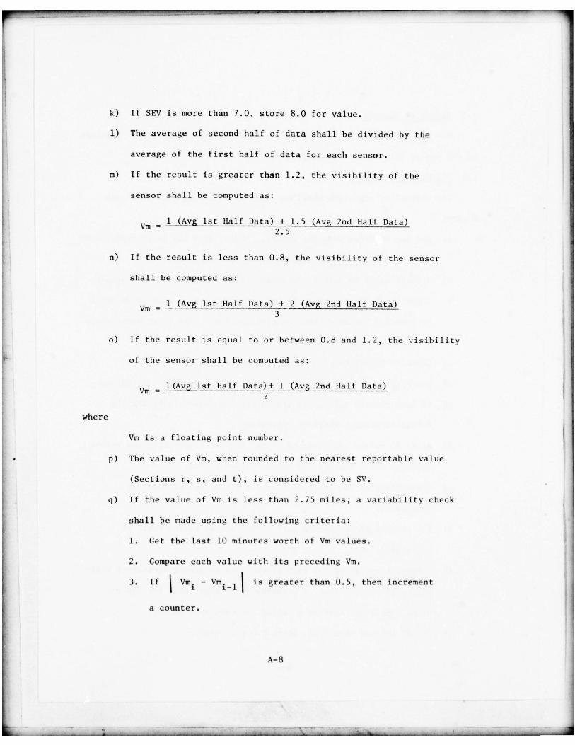
k) If SEV is more than 7.0, store 8.0 for value.
1) The average of second half of data shall be divided by the
average of the f i rst half of data for each sensor.
in) I f the r e su l t is grea te r than 1.2 , the v i s i b i l i t y of the
sensor shall be computed as:
— 1 (Avg 1st Ha l f Data ) + 1.5 (Avg 2nd Ha l f Data )
m — 2 . 5
n) If the result is less than 0.8, the visibility of the sensor
shall be computed as:
Vm 1 (Avg 1st Half Data) + 2 (Avg 2nd Half Data)3
o) If the resu l t is equal to or between 0.8 and 1.2 , the v i s i b i l i t y
of the sensor shall be computed as:
= l (Avg 1st Ha l f Data) + 1 (Avg 2nd H a l f Data )m
2
where
Vm is a floating point number.
p) The va lue of Vm , when rounded to the nearest r e p o r t a b l e value
(Sections r , s , and t ) , is cons idered to be SV.
q) I f the va lue of Vm is less than 2 . 7 5 m i l e s , a v a r i a b i l i t y check
shall be made using the f o l l o w i n g c r i t e r i a :
1. Get the last 10 m i n u t e s w o r t h of Vm values.
2. Compare each value with its preceding Vm .
3. If Vnhi — Vm . 1 is grea ter than 0.5, then incremen t
a counter.
A— 8
~~~~~~~~~~~~
.
~~~~~

- ____
4. If the counter is equal or greater than 3, report visibility
as variable .
5. Output a remark that the visibility is variable followed by
the maximum and minimum Vm values generated in the last 10
minutes . The remark must be of the fo l lowing fo rm:
VSBY Mm Value V Max Value
Example: VSBY 1/4Vll/2.
r) Any v i s ib i l i t y must be repor ted in the fo l lowing values:
0 , 1/4 , 5/16 , 3/8 , 1/2 , 5/ 8 , 3/4 , 7/8 , 1, 11/8 , 11/4 ,
13/8 , 11/2 , 15/8 , 13/4 , 17/8 , 2 , 21/4 , 21/2 , 3, 4 , 5 ,
6 , 7 and 8+ .
s) If the repor table value of Vm as obtained from Section r is
2 miles or less , use the following procedure . If this new Vm
has not changed by at least two r epor t ab le values f rom the pre-
viously reported SV , cont inue to use the previous SV as the
current SV.
t ) If the last reported SV was:
1. 2 1/4 , use 2 1/4 as the cu r ren t SV if the cur rent Vm is
between 2.01 and 2 . 4 9 ;
2. 2 1/2, use 2 1/2 as the cur rent SV if the cur rent Vm is
between 2.26 and 2.99;
3. 3, use 3 as the current SV if the current Vm is between
2.51 and 3.60.
Otherwise , use the reportable values as generated in
Sect ion l . 4 r .
A-9
L _ _ _ _ _ _ _ _ __ _ _ _ _

.•— — --. - - — — - ——-- - ~~~~~~~~~~~~~~~~~~~~~~~~~~~~~~~~~~~~~~~~~~~~ — -
u) A check shall be made to determine if a special message is re-
quired by using the following criteria:
If the present SV, when compared to the last Service “A”
visibility, meets any of the criteria listed in Section
1.2, a special counter must be incremented . If the counter
is incremented on two successive minutes , a special Service
“A” message must be generated and the counter set to zero .
v) The current SV wi l l be reported in the v i s i b i l i t y sect ion of the
Service “A” message.
w) Remarks, as generated , will be placed at the end of the Service
“A” message.
x) A new visibility observation will be generated each minute.
A- 10
~~~~~~~~~~~~~~~~~~~~~~~~~~~~~~~~~~~~~~~~~~~~~~~~~~~~~~~~~~~~~~~~~~~~~~~~~~~~~~~~~~~~~~~~~~~~~~~~~~~~~~~~~~~~~ ~~~ - - -~~~~~~—~~~~~ -~~~~~ -— ~~~~~ -~~~~~~--—~~~~~~~~ -~~ — - ---

—--- -- - --- - -~~~ - - - - -- --~~ ---~~ ~~~~~~~~~~~~~~~~~~~~~~~~~~~~~~~~~~~~~~ -~~~ —~~~--
THREE SENSOR VISIBILITY ALGORITHM
1. Visibility
The system shall include provisions for determining a representative
vis ibi l i ty fo r a selected area. The repor table ~~sibili ty val ues range from
1/4 miles to 8 miles . The output v i s ib i l i t y is cal led a preva i l ing v i s ib i l—
ity (PV) since it chooses the middle value from a three sensor network and
designates this value as PV. This choice of the middle value is the a lgor i thm
approximation to the FMH—l requirement of choosing the greatest visibility
which is a t t a i n e d or surpassed throughout at least half of the horizon circle.
1.1 Resolution
Visibility sensors shall determine visibility from “less than 1/4 mile ”
up to a range of 8 miles . Visibility of less than 1/4 mile is reported as 0
visibility.
1.2 Signlficant Changes In Visibility
The system shall provide for detertning and reporting when prevailing
visibility (PV) (rounded to reportable values), decreases to less than , or
If below , increases to equal or exceeds:
1. 3 miles.
2. 2 miles.
3. 1 1/2 miles.
4. 1 mile
5. All nationally published minima, applicable to the airport , listed
in the National Ocean Survey instrument approach procedure charts
or DOD f l i p s .
6. Values established locally because of their significance to local
aircraft operation .
A— l l
~
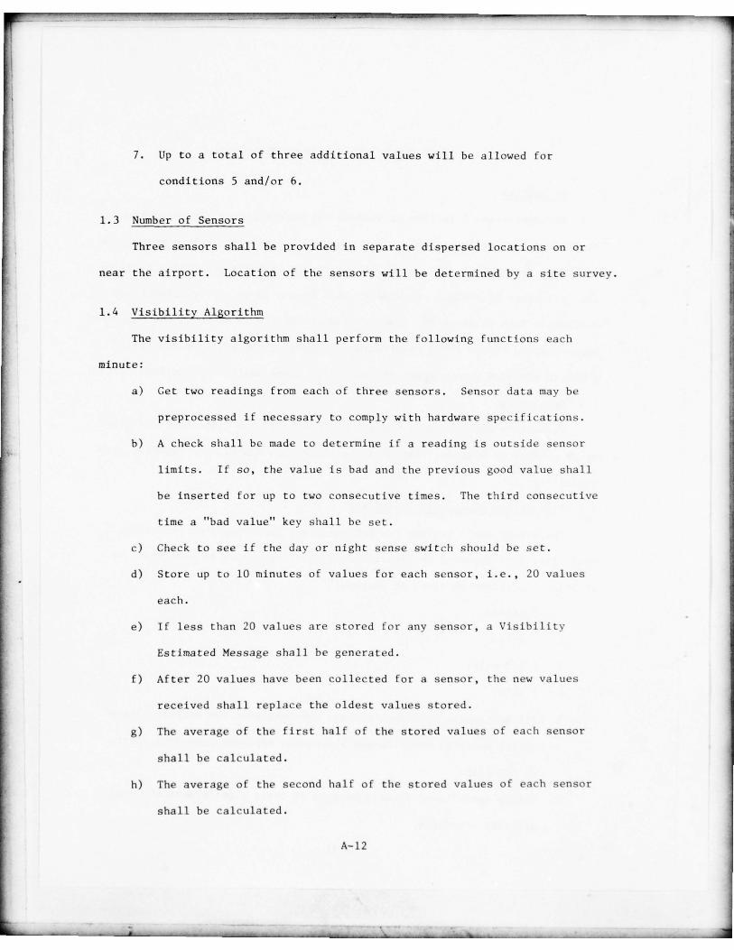
- ~~~~ — - - - r t - - - a r. ,~rrn’v~ ~--~~~~~~~~~~ -a~~~ -.
7. Up to a total of three additional values will be allowed for
conditions 5 and/or 6.
1.3 Number of Sensors
Three sensors shall be provided in separate dispersed locations on or
near the a i r p o r t . Location of the sensors wi l l be de te rmined b y a s i t e s u r v e y .
1.4 V i s i b i l i t y Al gor i thm
The v i s ib i l i t y a l g o r i t h m shal l p e r f o r m the following functions each
m i n u t e :
a) Get two read ings f rom each of three sensors. Sensor da ta may be
preprocessed if necessary to comply with hardware specifications.
b) A check shall be made to determine if a reading is outside sensor
l i m i t s . I f so , the va lue is bad and the previous good value shall
be inserted for up to two consecutive times. The third consecutive
time a “bad value” key shall be set.
c) Check to see if the day or night sense switch should be set.
d) Store up to 10 m inutes of val ues f or each sensor , i.e., 20 val ues
each.
e) If less than 20 values are stored for any sensor , a Visibilit y
Estimated Message shall be generated .
f ) A f t e r 20 values have been col lec ted fo r a sensor , the new values
received sha l l rep lace the oldest values s t o r ed .
g) The average of the f i r s t ha l f of the stored values of each sensor
shall be calculated.
h) The average of the second ha l f of the s tored va lues of each sensor
shal l be c a l c u l a t e d .
A- 12
~~ —-- - - - ~~~~~~~~~~~~~~~~~~~~~~~~ ..

-- -~r— - ~~~-
~~~~--—- - - - — - — - —----- - - -
- - - - - -- - —-__ - - -
I) Convert the reading fo r each set of data to sensor equivalent
v i s ib i l i t y (SEV ) in miles . A separate conversion for day and
ni ght conditions must be supplied for each type of sensor.
j) If SEV is less than 0.25, store 0.0 for value .
k) If SEV is more than 7 .0 , s tore 8.0 fo r value .
1) The average of second ha l f o f da ta shall be d iv ided by the average
of the first half of data for each sensor.
m) If the resul t is g rea te r than 1.2 , the v i s i b i l i t y of the sensor
shall be computed as:
- 1 (Avg 1st Half Data) + 1.5 (Avg 2nd Half Data)
2 .~
n) If the result is less than 0.8, the visibility of the sensor shall
be compu ted as:
= 1 (Avg 1st Half Data ) + 2 (Avg 2nd Half Data)
3
o) If the result is equal to or between 0.8 and 1.2, the visibility
of the sensor sha l l be computed as:
= 1 (jLvg lst Half Data ) + 1 (Avg 2nd Half Data )
2
where
V is a floating point number.
p) The mean v is ib i l i ty (Vm) shall be selected using the fol lowing
criteria
1. If three sensors, select central value .
2. If two sensors, select lower value
3. I f one sensor , select value .
4. I f no sensor , put in a f l a g to report v i s i b i l i t y data is missing .
A-l3
-- - - -— -

~ - ——- —
Th is val ue üf Vm , when rounded to the nearest reportable value
(Sections y, z and aa), is considered to be PV.
q) The lowest average visibility shall be obtained if tht- r~- is data
from all three sensors .
r) A remark shall be generated if the lowest visibility is less than
2.75 miles and if the mean vis ibilit y minus the lowest visibility
is greater than 0.5 mil es.
s) The remark shall st~it t that visibilit y is lowe r in a stated direc-
tion and give the value of the lowest visibilit y in ro~~• r t a bl e
values. The remark must be of the form :
VSBY Direction Value
Ex ampl e: VSBY NE 1 / 2
t) The hi ghest average v i s i b i l i t y shall be obtained if t h o r e is data
f rom all three sensors.
u) A remark shall be g e n e r a t e d i f the me an v i s i b i l i ty i s equa l t o or
less ‘ han 2.75 miles and if the highest visibility minu s the mean
visibilit y is greater than 0.5 miles.
v) The remark shall state that visibilit y is h ighe r in a s t a t e d d i r e
t ion , and give the va l ue of the h i g h e s t v i s i bi l i t y in r e p o r t a b l e
values. The remark must be in one ot t h ese t o rms:
VSBY rirection Value , when th ere i s higher visibilit y , only;
or VSBY Directi on I. Value L Direct ion H Value H , when there
are both hi gher and lower visibilit y . Examp l e: \ SBY Wl/2SE2 .
w) T f a remark is present for both higher and lower sector v i s i b i l i t
the remark for lower visibility will he reported first.
x) If the mean vi sibilit y (Vm) is less t h a n 2.75 miles , a vi r i a h i l i f
check shall be made using the following c r i t e r i a :
A-14
- - - ---- — - — -—— —-- ----~~- — —--

1. Get the last 10 minutes worth of Vm values.
2. Compare each value with its preceding Vm .
3. If I V m i — Vm 1 1 ~
is greater than 0.5, then increment
a counter.
4. If the counter is equal or greater than 3, report visibility
as variable.
5. Output a remark that the visibility is variable followed by
the maximum and minimum Vm values generated in the last 10
minutes. The remark must be of the following form :
VSBY Mm Value V Max Value
Example: VSBY l/4Vll/2.
y) Any visibility must be reported in the following values:
0, 1/4 , 5/ 16 , 3/8 , 1/2 , 5/8 , 3/4 , 7/8 , 1, 11/8 , 11/4 , 13/8 ,
11/2 , 15/8 , 13/4, 17/8 , 2, 2 1 / 4 , 2 1/2 . 3, 4, 5, 6, 7 and 8+ .
z) If the repor tab le val ue o f Vm as ob ta ined f ro m Sec tion y is 2
miles or less , use the following procedure . If this new Vm has
not changed by at least 2 reportable values from the previously
repor ted PV , continue to use the previous PV as the current PV.
aa) If the last reported PV was:
1. 2 1/4 , use 2 1/4 as the current PV if the current Vm is
between 2.01 and 2.49;
2. 2 1/2 , use 2 1/2 as the current PV if the current Vm is
between 2.26 and 2.99 ;
3. 3, use 3 as the current PV if the current Vm is between
2 .5 1 and 3.60.
Oth erwise , use the reportable values as generated In Section l.4y.
A-l5
.
~
- -- _;____ _____ _ _ -----—------— --— - --- — — — -—~~-~~~~-— - - -

ab) A check shall be made to determine If a special message Is re-
quired by using the following criteria:
If the present Vm (rounded to reportable values) when com-
pared to the last Service “A” visibility meets any of the
criteria listed in Section 1.2, a special counter must be
incremented. If the counter is incremented on two successive
m i n u t e s , a special Serv ice “A ” message must be genera ted and
the counter set to zero .
ac) The current PV will be reported in the visibility section of the
Serv ice “A” message .
ad) Remarks , as genera ted , w i l l be p laced at the end of the Service “A”
message . If two visi5ility remarks are generated , only one will be
reported. A “variable visibilit y ’ remark will have precedence over
“sector visibility. ”
ae) A new visibility observation is to be generated each minute.
A- 16
-

r ~~~~~~~~~~~~~~~~~~~~~~~~~~~~~~~~~~~~~~~~ ~~~~~~~~~~~~
--
APPENDIX B
CLOUD ALGORITHM
Comments on the Single Sensor Cloud Algorithm
1. The al gor i thm is essentially the single sensor AV—AWOS algorithm used
at PHF and updated by the October 1978 three sensor algorithm .
2. In the single sensor algori thm , we use recen cy we igh t ing to give grea ter
emphasis to the current cloud data . This is done by giving double weight
to the last 10 minutes of cloud data.
3. The adequacy of using a single sensor as opposed to a three sensor net-
work must be determined for each location by a site committee.
4. A generalized flow chart is attached .
8-1
__ j_*~ - - --- ~~~~~~~~~~~~~~~~~~~~~~~~~~~~~~~~~~~~~~~~~~~~~~~~~~ - — - —~~~~~~~~~~~~~~—

C/)
C
C ~— 0) >~ C
. E —I- L. ~~ Q
-~~~~ ~~~ ci’C) ~~
C~~~ CD 2
o +-~ -
‘.— --- -~~~~ ‘-, 0F’ ~ D — .C ~‘-~~ Cl)‘~-‘ W . o ~
>= (Y~ — el — ., ~~I—. I
~L~J0.. ~~ .
~~~~ ~‘ o-~ m r > Q) - - W . —- —
~~~~~~~~ ~~~~~ °- e ~~ —
L u) fl m c~ ( D E .2E 0 ‘O ~3 n E 0) E
if) • . ._ 0 Z _Jw
~~~
°0 I H~~
—
~~~~~~~~~~~~~~ o <~~~~~ c?(~~~~ ~~~~
I—
-_ -- ~~~~~~~~~~~~~--- - - - -~~~~~~~- -- - -~~~~~~~~

- — - - - ~~~-~~~~~~~~~~~ - — - -
Comments on the Three Sensor Cloud Algorithm
1. The algorl iim is essentially the algorithm as currently programmed In
AV—AWO S and used operationally at PHF.
2. In Section l.5m 2(2), we have made a technical correction to the — X pro-
gram. Instead of just adding .2 to each cloud layer for —X , we now
f i r s t de termine for each layer the amoun t of clo uds hidden by —X and
subtract the value from the cloud amount. The .2 obscuration is then
added to the corrected cloud amount.
3. In l.5q 12, we restricted the numbers of remarks added at the end of
the AV—AWOS message . In order to be added to the AV—AWOS message, each
remark must now be generated on three successive one minute observations.
When this condi tion is me t , a priority table is then used to output only
one cloud remark .
4. We have maintained the total obscuration program used at PHF. It has
serious limitations due to the lack of a vertical visibility sensor. An
alternative program would be to use the word OBSC for WAX , when appro-
priate , and not use a vertical visibility height value . For internal
use in the algorithm (to trigger specials, etc.), the vertical visibility
would be set at 100 feet.
5. The algorithm assumes all sensors are at the same height above MSL. De-
pending upon the siting at each location , it may be necessary to build
In a height correction factor.
6. Section l.5j is used as noIse suppression . Our tests have shown occa-
sional spurious noise generated by the RBC .
7. A generalized flow chart is attached .
B— 3
-
~
-
~
—- --~~~~~ a —~~~~ -~~~~ ~~~~~~~~~~~~~~~~~~~~~~~~

- -- ‘ — :V ; - — z ~ .- ~~~~~~~~~~~ ~ z. v rrr _ : ~~~~~~~~~~~~~
-_ -__ - _ - _ - - — — ------——- ——— ---—--- - —
I
I, III iiici) c 0
C/, 0-J cro —
H (/) -I— w —W 0< U) 9
Cr 0u > H
~-~tP1~1~:I1
_ _ _ _ __________________________

SINGLE SENSOR CLOUD ALGORITHM
1. Cloud Cover and Height
The system shall include provisions fo r determining the amount of cloud
cover and cloud heights in the general sensor area.
1.1 Acc uracy of Cloud Heights
Sensors shall be provided to determine cloud heights as follows :
+100 f eet f ro m 100 fee t to 1000 fee t ,
±10% from 1000 feet to 5000 feet ,
±20% above 5000 feet.
1.2 Number of Sensors
A single cloud height sensor shall be provided . A site survey will
determine the location of this instrument.
Horizon tal v isib ility and air tempera ture as de termined elsewhere in
the automated observation must also be supplied .
1.3 Cloud Cover
Cloud cover shall be determined to the nearest 0.1 coverage from 0.0
to 1.0.
1.4 Significant Changes in Cloud Cover
The system shall provide for the determination and reporting of changes
which meet the following criteria:
Ceil ing
The ceiling (rounded to reportable values) forms below , decreases to
less than , or if below , increases to equal or exceed :
8—S
~~1
_ _ _ _ _ --I--- — - - - - -- .—- i— -- —-- ~~~~~ -~~~---— - - —— --- - - ~ ---- -
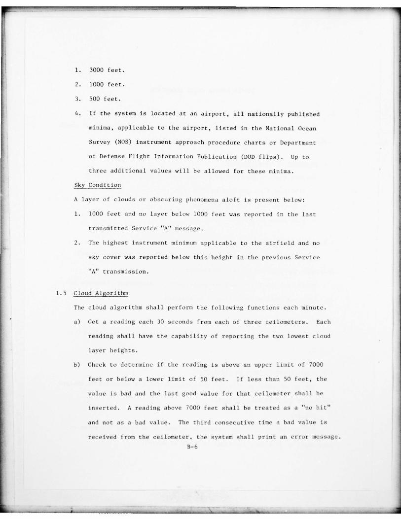
- -:-~~~~~~~ —------- ---— - - -— —-~~~~- --------- - I
1. 3000 feet.
2. 1000 feet.
3. 500 feet.
4. If the system is located at an airport , all na tion a l l y publ ished
minima , app li cable to the airport , listed in the National Ocean
Survey (NOS) instrument approach procedure charts or Department
of Defense Flight Information Publication (DOD fli ps). Up to
three additional values will be allowed for these minima .
Sky Condition
A layer of clouds or obscuring phenomena aloft is present below :
1. 1000 feet and no layer below 1000 feet was reported in tile last
transmitted Serviee “A” message.
2. The highest instrument minimum applicable to the airfield and no
sky cover was reported below this height in the previous Service
“A” transmission.
1.5 Cloud Algorithm
The cloud algorithm shall perform t h e following functions each minute.
a) Get a reading each 30 seconds from each of three ceilometers. Each
reading shall have the capability of reporting the two lowest cloud
layer heights.
b) Check to determine i the reading is above an upper limit of 7000
feet or below a lower limit of 50 feet. If less than 50 feet , the
value is bad and the last good value for that ceilometer shall be
inserted . A reading above 7000 feet shall he treated as a “no h it ”
and not as a bad value. The third consecutive time a bad value is
received from the cellometer , the system shall print an error message.
B— 6
-
~
-
~
-
~
- - - ~~~~~~~~~~~~~~~~~~~~~~~~~~~~~~~~~~~~~ _ _ _ _ _ _

r -- -- - - - —----------- - -- —— - - -
~~~~~
At that time , data from the ceilometer is excluded from any fur-
ther data processing , the ceilometer is considered as “off—the—air ”
and no further cloud message shall be generated .
c) The input value w i l l be the height in f e e t . Bin each input height
as f ollows:
Surface to 5000 feet: to nearest 100 feet ,
5000 feet to 7000 feet: to nearest even 200 feet (e.g.,
5000 , 5200 , 5400 . . . ).
This binned value shall be used in computing the cloud clusters.
However , the actual height value must be maintained .
d) Store up to 30 minutes of cloud heights , two heigh ts of each
ceilome ter each 30 seconds.
e) Tag the two lowest cloud heights from each cycle scan of the
ceilometer as follows :
1. Time of receipt.
2. Class of strike:
Class A = Only one cloud strike on that ceilometer scan
cycle or the hig her of two strikes.
Class B = The lower strike on a scan where two hits are
recorded.
f) Recency Wei ghting — To give greater emphasis to the more current
da ta , we give double weight to both hits and no hits in last 1/3
of data period. The actual hits are thus computed as the total
hits in the first 2/3 of the data period plus twice the hits in
the last 1/3 of the data period . The total possible hits are
computed using 2.67 times the minutes the ceilometer has been
B— 7
~
- -- . - -~~~~~~~~ - -~~~~~ - ~~~~~~~~~~~~~~~~~~~~~~~~~~~~~~~~~~~~ - - ---_ _ _ _ _

collecting valid data plus 1 t imes all the Class B h i t s in f i r s t
2/ 3 of data per iod p lus 2 times Class B hits in last 1/3 of data
period. These double weights are binned like regular data and
these values used in the remainder of the algorithm .
g) If less than 30 minutes of heights are available , estimate (E)
shall prefix a ceiling height. If 30 minutes of heights are
ava ilable , meas ured (N) shall pr efix a ceiling height.
h) If there is more than one height value recorded in the sampling
period , the values shall be tested and , i f needed , clustered
using the following criteria:
1. A check shall be made to determine if there are five or less
clusters (or bins).
2. If there are five or less clusters , go to Step i.
3. The values shall be ordered from lowest to highest heights .
4. The least square distances of all adjacent heights shall
be calc ulated
2 —
N ( T ) X N(K) X [H(J)—H(K) ]2
D N ( J ) + N ( K )
where:
D = Least square distance.
H = Cluster (bin) height.
N Number of cloud hits in that cluster.
5. The smallest least square distance shall be found.
6. If there are more than five clusters , the two clus te r-~ with
the smallest least square distance between them shall h€
combined .B— 8
.
~
----
~
—----— -*-------—-- —- -------- -- -— ~~~~—- - - ---— —~~~~~~~~~ ----- - —-“-- -

- -~~~~—~~~~~~~-- _ _ _ _ _- - -~~~~~
-- -
~~~~~~~~~~~
7. The c lus te r shall be combined as fol lows for height :
H(L ) - [N(J) X H(J)) + [N(K) X H(K)]
- N(J) + N (K)
and as follows for number of samples :
N(L ) = N ( J ) + N ( K )
8. The range of height values in a cluster shall be retained .
These are the maximum and minimum values included in the
cluster and are actual , not binned , values.
9. The H(L) and N(L) cluster shall replace the 1-1(J) , H(K) ,
N (J) , and N(K) clusters.
10. The clustering process shall return to Step 1 above and
continue .
I) Af ter the clustering has been completed , a test shall be run to
determine If clusters from the same ceilometer can be combined :
1. Group the clusters in ascending order.
2. Compute the height difference of all adjacent clusters.
3. If lowest height of pair is less than 1000 feet and the dif-
ference be tween he igh ts is 250 fee t or less , combine the clusters;
if no t , go to the next height.
4. If lowest height of pair is greater than 1000 feet and the dif-
ference between heights is 350 fee t or less , combine the clusters;
if not , go to the next he ight .
5. If lowest height of pair is greater than 3000 feet and the dif-
ference between heights is 450 feet or less , comb ine the clusters;
if not , go t O the nex t h e i g h t .
B—9
- - --- - - - - - --~~~~~~~~~~~~~~~~~~~~~-- -~~~~~~~~- ---~~ -- --

6. If the lowest height of pair is 5000 feet or higher and the
d i f f e r e n c e between he ights is 600 f eet or less , combine the
clusters; if not , go to next height.
7. The c lus ters are combined b y the f o l l o w i n g fo r h e i g h t :
1-1(L) — [H(J) N(Jfl + [11(K) N (Kfl
— N ( J ) + N ( K )
and a s
N ( L ) = N ( J ) +
fo r the number of samples .
8. When two clusters are combined , the range of value of the
cluster shall be maintained; the new cluster shall replace the
two which were combined ; the c l u s t e r s reordered and the process
of combining continued.
9. A l l a d j a c e n t p a i r s s h a l l be examined u n t i l no f u t u r e c m b i n i n g
is required.
j ) At the end of this process if m v cluster has five h its or less ,
this cluster is not considered any further in the program and the
number of hits is not added to any other cluster. However , the
total possible hits (as calculated in Section l.5e) are not reduced .
All cluster heights are now rounded to:
Surf ace — 5000 feet: nearest 100 feet
5000 feet to 7000 feet: nearest 500 feet
(5000 , 5500 , 6000 , etc.).
k) The sky cover shall be cal culated by using the following crit e ria:
1. The total possible hits shall be obtained from Section l.Se.
B-b
~~~~~~ ~~~~~~~~~~~~~~~~~~~~~~~~~~ -~~- -- - —-- - - - - - --— -~~ -—--- -- -----~~~- — -

- ,.~~~~~-~--—- --- _________________________
2. The cloud cover f a c t o r (R L ) shall be ca lcula ted using the
following criteria for each layer starting with the lowest
cluster (layer):
— L~l (Tota l Number of Layer Hits )
— Total Poss ib l e H i t s
where n is the cluster order number starting from the lowest
layer. For the subsequent (i.e., L> l) layer s, the summation
pr inc i p le f rom FMII—l is applied. That is , i f a lower layer
at h e i g h t h 1 has 25 hits , and a higher layer at height h2 has
13 hits; RL
fo r h~ would be computed using 38 divided by the
total possible hits.
3. If less than five hits from all ceilometers “CLR BLO 70” shall
shall be stored .
‘ . If five or more hits and < 0.06 fo r a l l L , “CLR BLO 70 ” shal l
be stored and a remark of “Few Clo uds ” and the height of the
cluster shall be stored. Examp le : FEW CLDS 55 for few clouds
at 5500 feet.
5. I f R L < 0.55 , heig ht and “ s ca t t e r ed” shall be st o r e d .
6. If RL
< 0.87 , heIght and “broken ” shall he stored .
7. If R.L > 0.87 , height and “overcast ” shall be stored.
8. If more than one layer has a R.L > 0.87 , a remark of higher
clouds visibl e shall be stored. Example: FUR CLDS VSB .
9. For the lowest scattered , broken , and overcast layers . only ,
divide the total number of Class B strikes up to and includ i-
that layer by the total number of (non—zero) hit s or t o mn
B—li
—- — -~~ - - --- -- -- - ~~~~~ — -- - -

r ~~~ AD—A072 119 NATIONAL WEATHER SERVICE SILVER SPRING MO FIG k/2AVIATION AUTOMATED WEATHER OBSERVATION SYSTEM IAV — AWOS ) • (U)MAR 79 DOT—FA 73WA I—sekF UNCLASSIFIED FAA— RD—79—63
2~~~?40O~ 2I 9
END
____________ _________________________ 0
9 79
p

111111.0 Lj ~ 2 2L 3.5
•1 4 L.~Iu. 11112.0I.’ ffll~~
• ~h1llIh25

including that layer. Call this ratio C. If C > 0.5, store
“thin” (—) in front of SCT, BKN, or OVC as appropriate.
1) A test shall be made to determine if the ceiling is variable.
The test shall use the following criteria :
1. If there is a broken or overcast layer, not classified as
thin (e.g., W2X is not considered a ceiling layer for van —
ability) below 3000 feet , its standard deviation , using
actual , not binned values , shall be calculated :
SD=~~~~~~N E H2 _ (E H)
2
where H is the individual height values that are clustered
into the layer.
2. If there is no broken or overcast layer below 3000 feet , the
variability test Is complete.
3. If the height is 1000 feet or below and the standard deviation
greater than 200, a remark shall be queued .
4. If the height is between 1000 and 2000 feet and the standard
• deviation is greater than 300, a remark shall be queued .
5. If the height [s greater than 2000 feet and the standard
deviation greater than 400 feet , a remark shall be queued.
6. If the remark is queued 1 minute in a row, a remark of ceiling
variable with minimum and maximum heights (the highest and
lowest binned values clustered into that layer) shall be
reported and the queue counter set to zero. The form of the
remark must be CIC MIN Height V MAX Height. Heights must be
reported in hundreds of feet. Example: CIG 15V20.
B— 12
,~~~~~ - -~~~~~~

in) A check shall be made to determine if the sky is obscured. If the
visibility (yin) as furnished elsewhere in the automated observation
is 1.8125 miles or below and the cloud sensor has 30 minutes of
data, scan last 10 minutes of cloud data.
1. If there are less than five cloud hits in the last 10 minutes
output as cloud cover/height —
WAX,
where:
A 1 if visibility is < 1/4 mile
2 if visibility is > 1/4 mile
or < 1.5625 miles
7 if visibility is > 1.5625 miles and < 1.8125 miles
and if the air temperature input is < 36°F.
Otherwise continue to Step n.
A is the vertical visibility (in hundreds of feet) and is
considered the ceiling height.
2. If there are five or more cloud hits within the last 10 min-
utes, and if the visibility is < 1.5625 miles, or if the air
temperature is < 36 F and the visibility is < 1.8125 miles:
1) If ILL < .06 for all layers, the cloud algorithm shall
read —X and nothing else will be reported in the
cloud group.
2) If > .06, multiply each cloud layer amount by .2.
Subtra~~ these values from their respective cloud
layers. Add .2 to each cloud layer and use these new
cloud layer amounts in the subsequent steps. Prefix
B— 13
-—__
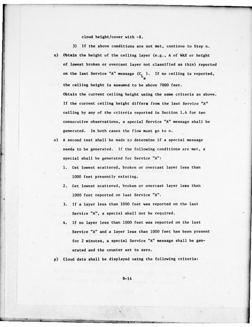
— - - ~=--
cloud height/cover with —X.
3) If the above conditions are not met, continue to Step n.
n) Obtain the height of the ceiling layer (e.g., A of WAX or height
of lowest broken or overcast layer not classified as thin) reported
on the last Service “A” message (CL). If no ceiling is reported ,
the ceiling height is assumed to be above 7000 feet.
Obtain the current ceiling height using the same criteria as above.
If the current ceiling height differs from the last Service “A”
ceiling by any of the criteria reported In Section 1.4 for two
consecutive observations, a special Service “A” message shall be
generated. In both cases the flow must go to o.
o) A second test shall be made to determine if a special message
needs to be generated . If the following conditions are met , a
special shall be generated for Service “A”:
1. Get lowest scattered , broken or overcast layer less than
1000 feet presently existing.
2. Get lowest scattered , broken or overcast layer less than
1000 feet reported on last Service “A”.
3. If a layer less than 1000 feet was reported on the last
Service “A”, a special shall not be required .
4. If no layer less than 1000 feet was reported on the last
Service “A” and a layer less than 1000 feet has been present
for 2 minutes, a special Service “A” message shall be gen-
erated and the counter set to zero.
p) Cloud data shall be displayed using the following criteria :
B— 14

1. If obscured , the decision table in m.l shall be reported.
2. If clear, It shall be reported as “CLR BLO 70” and the
remark “few cids hh” added , if appropriate.
3. If one layer, it shall be reported.
4. If two layers, they shall be reported except only one
overcast is reported.
5. If three layers, they shall be reported except only one
overcast is reported.
6. The reporting shall be from the lowest to the highest layer.
7. If there are more than three layers, a total of three layers
shall be reported in the following order or precedence:
a. The lowest scattered (SCT) layer not classified as thin.
b. The lowest broken (BKN) layer.
c. The lowest “thin” SCT layer.
d. The overcast (OVC ) layer.
e. The lowest “thin” BKN layer.
f. A “thin” OVC layer.
g. The second lowest SCT layer.
h. The second lowest BXN layer.
i. The highest BXN layer.
j. The highest SCT layer.
8. 1) If lowest BKN layer has a ratio between .55 and .59,
add in remarks “BKN VRBL SCT.”
2) If highest BKN layer reported has a ratio between .85
and .87, add in remarks “BKN VRBL OVC.”
3) If OVC layer reported has a ratio between .87 and .89,
add in remarks “OVC VRBL BKN.”
3-15
~~~~~~~~~ -~-~~~--~ ~~~~ ~~~~~~~~~~~~~~~~~~~~~~~~~~~~~~~~~ ~~~~~~~~~~~~~~~ ~~~~~~ ~~‘~~~~~~~~ - ‘ •~~~~~~- - - -

9. For lowest BKN or OVC layer prefix height value with an M or E
as appropriate (e.g., Ml2 BKN).
10. —X shall precede the cloud layers as appropriate from m.2.
11. Each layer must be reported with its heights in reportable values
in front of the layer type. Example: scattered clouds at 800
feet and broken clouds at 3200 feet are reported a 8 SCT M32 BKN.
A blank shall separate the height and the amount designator and
will also be used to separate successive cloud groups.
12. Remarks, as generated by the algorithm, shall be added at the end
of the observation message.
Each remark must be generated on at least three successive one
minute observations before it will be added to the end of the
output message. Only one cloud remark shall be added to each
message. The priority of these remarks are:
FEW CLD HI-I (Section 1.5 k 4)
CIG MIN V MAX (Section 1.5 1 6)
BKN VRBL SCT (Section 1.5 p 8(1))
BKN VRBL OVC (Section 1.5 p 8(2))
OVC VRBL BKN (Section 1.5 p 8(3))
HIR CLDS VSB (Section 1.5 k 8).
q) A new observation will be generated each minute.
8—16
~1’~~~~~ — - —

THREE SENSOR CLOUD ALGORITHM
1. Cloud Cover and Height
The system shall include prov isions for de termining the amount of
cloud cover and cloud heights in the general airport area.
1.1 Accuracy of Cloud Heights
Sensors shall be provided to determine cloud heights as follows:
±100 feet from 100 feet to 1000 feet,
±10% from 1000 feet to 5000 feet,
• ±20% above 5000 feet.
‘ I 1.2 Number of Sensors
Three cloud height sensors shall be provided located in separate
dispersed locations. A site survey will determine the location of the
instruments. Visibility and temperature as determined elsewhere in the
automated observation must also be supplied. Sensors should be corrected
to the same height.
1.3 Cloud Cover
Cloud cover shall be determined to the nearest 0.1 coverage from 0.0
to 1.0.
1.4 Significant Changes in Cloud Cover
The system shall provid, for th. determination and reporting of changes
which meet the following criteria :
Cell m lTh. ceiling (rounded to reportable values) forms below, decreases to
less than, or if below , increases to equal or exceed :
1—17
~~~~~~~~ - — - _______
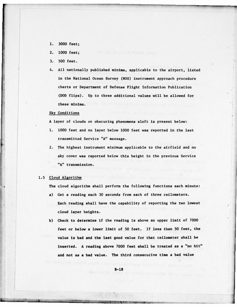
1. 3000 feet;
2. 1000 feet;
3. 500 feet.
4. All nationally published minima, applicable to the airport, listed
in the National Ocean Survey (NOS) instrument approach procedure
charts or Department of Defense Flight Information Publication
(DOD flips). Up to three additional values will be allowed for
these minima.
Sky Conditions
A layer of clouds or obscuring phenomena aloft is present below:
1. 1000 feet and no layer below 1000 feet was reported in the last
transmitted Service “A” message.
2. The highest instrument minimum applicable to the airfield and no
sky cover was reported below this height in the previous Service
“A” transmission.
1.5 Cloud Algorithm
• The cloud algorithm shall perform the following functions each minute :
a) Get a reading each 30 seconds from each of three ceilometers.
Each reading shall have the capability of reporting the two lowest
cloud layer heights.
b) Check to determine if the reading is above an upper limit of 7000
feet or below a lower limit of 50 feet. If less than 50 feet, the
val ue is bad and the last good valu e for that ceilome ter shall be
inserted. A reading above 7000 feet shall be treated as a “no hit”
and not as a bad value. The third consecutive time a bad value
8—18
— ._____I — — - .~~~~~~~~-~~~~ ~~~~~~~~ _______ —

_ _ _ ---- ~~~- --- -~~ .- -- ---~~ -~~~~~~~~- -~~--—~~~
is rece ived from the same cellometer , the system shall print an
error message. At that time, data from this ceilometer is excluded
fro m any further data processing, the ceilometer is considered as
“off—the—air” and the total possible number of hits is reduced
accordingly.
c) The input value will be the height in feet. Bin each input
heights as follows:
Surface to 5000 feet: to nearest 100 feet.
5000 feet to 7000 feet: to nearest even 200 feet (e.g.,
5000, 5200, 5400 ...).
This binned value shall be used in computing the cloud clusters.
d) Store up to 30 minutes of cloud heights, two heights of each
ceilometer each 30 seconds.
e) Tag the two lowest cloud heights from each cycle scan of each
ceilometer as follows:
1. Ceilometer from which it originated.
2. Time of receipt.
3. Class of strike:
Class A — Only one cloud strike on that cellometer
scan cycle or the higher of two strikes.
Class B — The lower strike on a scan where two hits
are recorded.
The total possible hits shall be calculated. The total possible
hits is two times the minutes ceilometer 1 has been collecting
valid data, plus two times the minutes ceilometer 2 has been
collecting valid data , plus two times the minutes ceilometer 3
3—19
I. ~~~~~~~~~~~~~ —~~~ -- ~~~~~~—~ --.- - ~~~~~~~~~~~~~~~~~~~~~~~~~~~~~~~~~ ‘~~~~~ - ~~~~~ ~~-~~~ -~‘-~~~ - —

has been collecting valid data, plus the number of hits from
the second level from all three ceilometers.
f) If less than 30 minutes of heights are available from any sensor,
estimate (E) shall prefix a ceiling height.
g) If 30 minutes of heights are available from all sensors, measured
(M) shall prefix a ceiling height.
h) If there is more than one height value recorded from a ceilometer
during the sampling period , the values shall be tested and, if
needed , clustered using the following criteria for each ceilometer
independently:
1. A check shall be made to determine if there are five or
less clusters (or bins).
2. If there are five or less clusters, go to Step i.
3. The values shall be ordered from lowest to highest heights.
4. The least square distances of all adjacent heights shall be
calculated -
2 N(J) X N(K) X EH(J) — H(Kfl2
D ~~N(J)+ N(K)
where:
D — Least square distance.
H — Cluster (bin) height.
N — Number of cloud hits in that cluster.
5. The smallest least square distance shall be found.
6. If there are more than five clusters, the two clusters with
the smallest least square distance between them shall be
combined.
B— 20
‘—~~~ ----~~~~~~--- -—
~ -. ——-—~~~~~~ - —----— . ,. ~~~~~~~~~~~~~~ -~ —~~--~~~~~ -~~ -

7. The cluster shall be combined as follows for height:
11(L) — IN(J) X 11(J)] + (N(K) X 11(K)]
N(J ) + N (K)
and as follows for number of samples
N(L) N(J) + N(K).
- ! 8. The range of height values in a cluster shall be retained.
• These are the maximum and minimum values included in the
cluster and are actual, not binned , values.
9. The H(L) and N(L) cluster shall replace the 11(J), 11(K), N(J) ,
and N(K) clusters.
10. The clustering process shall return to Step 1 above and
continue.
1) After the clustering has been completed , a test shall be run to
determine if clusters from the same ceiloineter can be combined.
The test shall use the following criteria for combining :
1. Group the clusters in ascending order.
2. Compute the height difference of all adjacent clusters.
3. If lowest height of pa ir is less than 1000 feet and the
difference be tween heights is 250 feet or less, combine the
clusters; if not, go to next height.
4. If lowest height of pair is grea ter than 1000 fee t, and the
difference between heights is 350 feet or less, combine the
clusters ; if not , go to next height .
5. If lowest height of pair is greater than 3000 feet, and the
difference between heights is 450 feet or less, combine the
clus ters; if not, go to next height.
8—21
--~.- ~~. - - - --—- -—- -- - - -
—~~~~~~~~ - r-

_ _ _ _________ _ _ _ _ - ----- --~~~~~ - - ~~~~--
6. If the lowest height of pair is 5000 feet or higher and
the difference between heights is 600 feet or less, combine
the clusters; if not, go to next height.
7. The clusters are combined by the following for height:
H L) — (H(J).N(J)] + [H(K).N(K)]
N (J) + N(K)
and as follows for number of samples:
N(L) — N(J) + N(K).
8. When two clusters are combined the range of value of the
cluster shall be maintained, the new cluster shall re place
the two which were combined, the clusters reordered and the
process of combining continued .
• 9. All adjacent pairs shall be examined until no future com-
bining is required.
j) Af ter the combining process has been completed , a test shall be
run to de termine if clusters from the differen t ceilometers can
be combined. To do this, repeat Step i using as input the
• clusters from all ceilometers.
At the end of this process, if any cluster has f ive hits or less,
- .~ this cluster is not considered any further in the program and
the number of hits is not added to any other cluster. However,
the total possible hits (as calculated in Section l.5e) are not
reduced. All cluster heights are now rounded to:
Surface — 5000 feet: nearest 100 feet.
5000 feet to 7000 fee t : neares t 500 feet
(5000 , 5500 , 6000 , etc.). .
8—22
~~~~~~~~~~~~~~~~~~~~~~~~~~~~~ •—~~--- - - - - - • -—-, __ _ _ __ _ _ _ _ i _ .---~•- -~~~ • :~~~~~~~~~~~~ _~~~~~~
- ~~~~~~~~~~~~~~~~ — -______

- - — - - ~~~~~~____ — -
k) The sky cover shall be calculated by using the following criteria :
1. The total possible hits shall be obtained from Section l.5e.
2. The cloud cover factor (R.L) shall be calculated using the
following criteria for each layer, starting with the lowest
cluster (layer)
= L~l (Total Number of Layer Hit~~RL (Total Possible Hi t s )
where
n is the cluster order number starting from the lowest layer.
For the subsequent layers (i.e., L>l), the summation principle
from FMH—l is applied . That Is, if a lower layer at height h1
has 25 hits, and a higher layer at height h2 has 13 hits , RL
for
h2 would be computed using 38 divided by the total possible hits.
3. If less than five hits from all ceilometers , “CLR BLO 70” shall
be stored.
4. If five or more hits and RL
< 0.06 for all L, “CLR BLO 70” shall
be stored and a remark of “Few Clouds” and the height of the
cluster shall be stored . Example: FEW CLDS 55 for few clouds
at 5500 feet.
5. If < 0.55, height and “scattered” shall be stored.
6. If RL
< 0.87, height and “broken” shall be stored .
7. If ILL > 0.87, height and “overcas t” shall be stored.
8. If more than one layer has a RL
> 0.87, a remark of higher clouds
visible shall be stored . Example: HIR CLDS VSB.
9. For the lowest scattered , broken , and overcast layers, only,
• divide the total number of Class B strikes up to and including
B—23
_______________________________________________________ ~~~~~~~~~~~~~~~~~~~~~~~~~~~~~~~~

r
- - - -_ _ _ _
that layer by the total number of (non—zero) hits up to
and including that layer. Call this ratio C. If C > 0.5,
store “thin” (—) in front of SCT, BKN , or OVC as appropriate.
1) A test shall be made to determine if the ceiling is variable. The
test shall use the following criteria:
1. If there is a broken or overcast layer, not classif ied as thin
(e.g., W2X is not considered a ceiling layer for variability),
below 3000 feet, its standard deviation, using actual, not
binned , val ues shall be calcula ted:
SD • ~~ ~~~~~NE 112 — (Z H) 2
where H is the individual height values that are clustered
into the layer.
2. If there is no broken or overcast layer below 3000 feet, the
variability test is complete.
3. If the height is 1000 feet or below and the standard deviation
grea ter than 200, a remark shall be queued.
4. If the height is between 1000 and 2000 feet and the standard
devia tion is grea ter than 300, a remark shall be queued .
5. If the height is greater than 2000 feet, and the stand ard
dev iation grea ter than 400 feet, a remark shall be queued.
6. If the remark is queued 1 minute in a row, a remark of ceiling
variable with minimum and maximum heights (the highest and
lowest binned value that was clustered into that layer) shall
be reported and the queue counter set to zero.
3—24
- - - - —- - ---- - — •-~~------ ------ _ _ _ _-----
~~
- - — - • -

The form of the remark must be CIG MIN Height V MAX Height.
Heights must be reported in hundreds of feet. Example:
d c lSV2O.
m) A test shall be made to determine if the ceiling is lower and/or
higher over the various ceilometers. The following steps must
be completed :
1. If there is a broken or overcast layer not classified as thin
and all three ceilometers are operational for 30 minutes, the
test is made; if not, the test is bypassed.
2. Get the last half of the data from each ceilometer within
the range of the ceiling layer (lowest broken or overcast
layer not classified thin).
3. Compute the average height of the last half of data in this
ceiling layer for each ceilometer. If any ceilometer does
not have three or more hits, the high and low tests (4 — 9
below) shall be omitted.
4. Get the lowest average height.
5. Get the highest average height.
6. If the lowest average height and the clustered height of the
ceiling layer difference is more than 200 fee t, a lover sector
exists.
7. A remark is generated that the ceiling is lower in the direc-
tion that the ceilometer is located from the airport. Format
of remark CIG LWR direction. Example: CIG LWR NW.
8. If the highest average height is greater than 200 feet dif-
feren t from the clus tered heigh t, a higher ceiling exists.
B—25
- ~~~~~~~~~~~~~~~~~~~~~~~~~~~~~~~~~~~~~~~~ -.•— •—.—~ ——~~~~~~~~~~~~~~~ -~~- - - -~- - -~ - • - -•~~~~ - - - - - — - ~ - — -——-- - -
- .~~L- ______ • - -— ~~~~~~~~~~~~~~~~~~~~~~~~~~~ ~~~ ‘ L ~~~~~’~~~~~ ! ~~~~~~~~~ .~~~~~~~~~ - ~~~ -

• - ---—--— -- - - — - - -~~~~~~~z~~:~~~~~~-~~~~
-•- - - -•-----••--•----- - — - —--• - -----—-•-•--- - ‘~1~
9. A remark is generated that the ceiling is higher in the
direction that ceilometer is located from the airport.
Format of remark CIG HIR direction. Example: CIG HIR SE.
Used only if 7 is not used.
n) A check shall be made to determine if the sky is obscured. If
the visibility (Vm) as furnished elsewhere in the automated obser-
vation is 1.8125 miles or below, and any one of the cloud sensors
has 30 minutes of da ta, scan last 10 minutes of cloud data.
1. If there are less than five cloud hits (from all ceilometers)
in the last 10 minutes output as cloud cover/height —
WAX ,
where :
A — 1 if visibility is < 1/4 mile
2 if visibility is > 1/4 mile
and < 1.5625 miles
7 if visibility is > 1.5625 miles and < 1.8125 miles
and if the air temperature input is < 36°F.
Otherwise continue to Step o.
A is the vertical visibility (in hundreds of feet) and is
considered the ceiling height.
2. If there are five or more cloud hits (from all ceilometers)
within the last 10 minutes, and if the visibility is < 1.5625
miles, or if the air temperature is < 36°F and the visibility
is < 1.8125 miles:
(1) If L < .06 for all layers, the cloud algorithm shall
read —X and nothing else will be reported in the cloud
group.• 8—26

- ---—- - - •------- --~~~— ~~~
(2) If ILL > .06, multiply each cloud layer amount by .2.
Subtract these values from their respective cloud layers.
Add .2 to each cloud layer and use these new cloud layer
amounts in the subsequent steps. Prefix cloud height/cover
with -X.
3. If the above conditions are not met , continue to Step o.
o) Obtain the height of the ceiling layer (e.g., A of WAX or height
of lowest broken or overcast layer not classified as thin) re-
ported on the last Service “A” message (CLa ). If no ceiling is
repor ted , the ceiling height is assumed to be above 7000 feet.
Obtain the current ceiling height using the same criteria as
• above. If the current ceiling height differs from the last Ser-
vice “A” ceiling by any of the criteria reported in Section 1.4
for two consecutive observations, a special Service “A” message
shall be generated. In both cases, the flow must go to p.
p) A second test shall be made to determine if a special message needs
to be generated . If the following conditions are met , a special
- •
message shall be generated for Service “A”:
- •.
~ 1. Get lowest scattered , broken or overcas t layer less than 1000
feet presently existing.
2. Get lowest scattered , broken or overcast layer less than 1000
fee t repor ted on las t Service “A”.
3. If a layer less than 1000 feet was reported on the last Service
“A”, a special message shall not be required .
4. If no layer less than 1000 feet was reported on the last Ser—
vice “A” and a layer less than 1000 feet has been present for
8—27
- !~— . -~— - --~~—‘.— ~~—_ ~~~~~~~~~~~~~~~~~~ - -—-.-—-~~~~~: J 1 L rLX : ~~~~•. ~~~
—~~ ---— • -~~~ - . • .. ~~~~~~~~~~~~~~~~~~~~~~ ~~~~~~~ ~~~~~~~~~~

— — —
— • —- • • — - --- - -•--- • - — --- ——— • — — ---• •-•- -—- -—-—--——.
~
— -
2 minutes, a special Service “A” message shall be genera ted
and the counter set to zero.
q) Cloud data shall be displayed using the following criteria:
1. If obscured, the decision table in n.1 shall be reported.
2. If clear, it shall be repor ted as “CLR BLO 70” and the remark
“few clds hh” added , if appropriate.
3. If one layer, it shall be reported.
4. If two layers, they shall be reported except only one over—
cast is reported.
5. If three layers, they shall be reported except only one over-
cast is reported. -
/
-• 6. The reporting shall be from the lowest to the highest layer.
7. If there are more than three layers, a total of three layers
shall be reported in the following order or precedence:
a. The lowest scattered (SCT) layer not classified as
thin.
b. The lowest broken (31(N) layer.
• c. The lowest “thin” SCT layer.
d. The overcast (OVC ) layer.
e. The lowest “thin” BKN layer.
f. A “thin” OVC layer.
g. The second lowest SCT layer.
h. The second lowest BKN layer.
i. The highest BKN layer.
j. The highest SCT layer,
3—28
• • -~ --- --- •—• -— —‘
~--- -=—
-~~~~~~~-~-—- ~~~~~~~~~~~~~~~~~~~~~~~~~~~~~~~~~~~~~~~~~~ — - -—~~---~~~-----—- -—-- T-
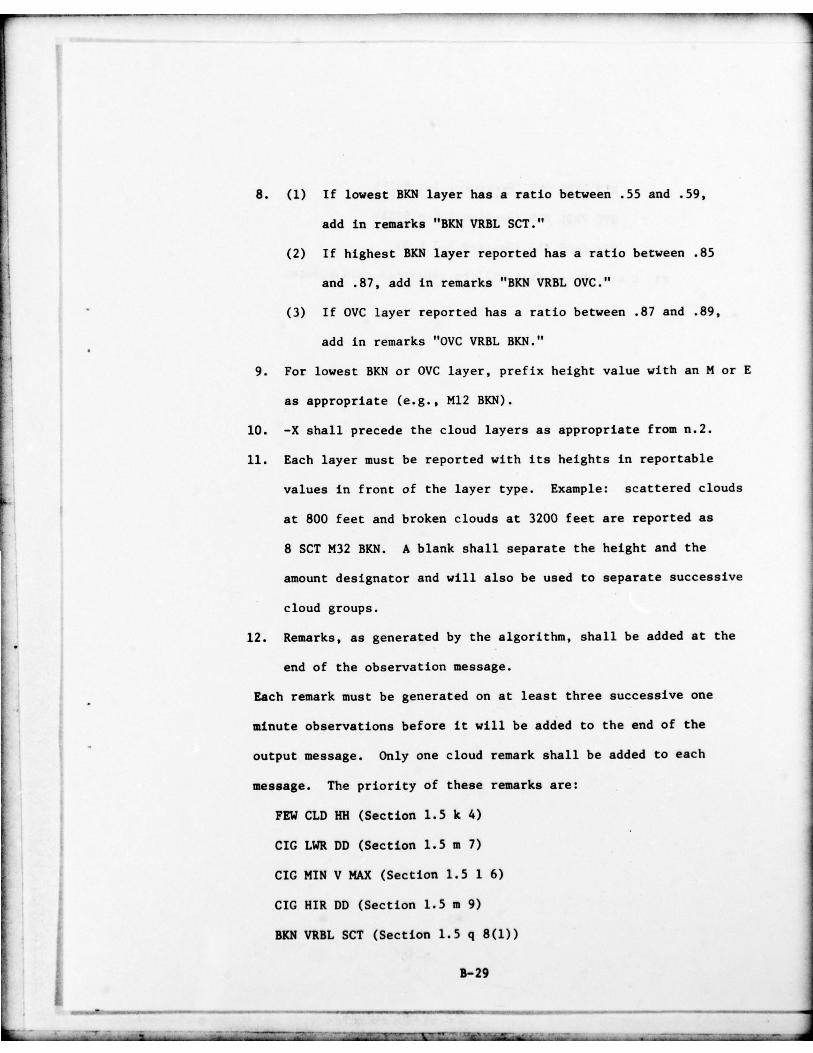
8. (1) If lowest BKN layer has a ratio between .55 and .59 ,
add in remarks “BKN VRBL SCT .”
(2) If highest BKN layer reported has a ratio between .85
and .87 , add in remarks “BKN VRBL OVC .”
(3) If OVC layer reported has a ratio between .87 and .89 ,
add in remarks “OVC VRBL BKN.”
9. For lowest BKN or OVC layer, prefix height value with an M or E
as appropriate (e.g., Ml2 BKN).
10. —X shall precede the cloud layers as appropriate from n.2.
11. Each layer must be reported with its heights in reportable
values in front of the layer type. Example: scattered clouds
at 800 feet and broken clouds at 3200 feet are reported as
8 SCT M32 BKN . A blank shall separate the height and the
amount designator and will also be used to separate successive
cloud groups.
12. Remarks, as generated by the algorithm, shall be added at the
end of the observation message.
Each remark must be generated on at least three succesaive one
minute observations before it will be added to the end of the
• output message. Only one cloud remark shall be added to each
message. The priority of these remarks are:
FEW CLD 1111 (Section 1.5 k 4)
CIG LWR DD (Section 1.5 m 7)
CIG MIN V MAX (Section 1.5 1 6)
• CIG HIR DD (Section 1.5 m 9)
BKN VRBL SCT (Section 1.5 q 8(1))
3—29
• - - - - -— —.--—-• -- - ---- -• • •- -- -
______________________________________________ v •~~~~-~~
- —~~-~~~—-~~~~~~~ - • --—--~-~~ . - - - ~~~~~~~~~~~~~~~~~

81(11 VU!. OVC (Section 1.5 q 8(2))
OVC VRBL 81(11 (Section 1.5 q 8(3))
HIR CLDS VSB (Section 1.5 k 8).
r) A new observation will be generated each minute.
3—30
_ _ _ _ _ _ _ _ _ _
- - ~~~~~~~~~~~~~~~~~~~~~~~~~~~~ ~~~! ~~~~~~~~~~~~~~~~~~~~~~~~~~~~~~~

APPENDIX C
AV—AWOS User Assessment Plan Results
Equipment Development Laboratory• System. Development Office
Na t ional Weather ServiceSilver Spring, Maryland
November 1978
~~~~~~
-_ _ _ _ _ _ _ _ _ _ _ _ _ _ _ _ _ _ _ _

1. Introduction
The purpose of the AV—AWOS User Assessment Plan at Patrick HenryAirport was to obtain user reaction/acceptability of an automatedweather observation. FAA’s National Aviation Facilities ExperimentalCenter and NWS’s Test and Evaluation Division and Equipment DevelopmentLaboratory prepared a questionnaire for use to survey the users of theAV—AWOS observation. A copy of this questionnaire is shown in figure 1.The questionnaire was distributed to the following user groups duringthe AV—AWOS test period (January — May, 1978) at Newport News, Virginia:
1. General Aviation Pilots2. Air Carrier Pilots, Dispatchers and Forecasters3. FSS Briefer.4. Air Traffic Controllers5. NWS and Military Forecasters/Observers
Results from the questionnaires were tabulated by EDL and are presentedin the following section.
The user groups listed in the first question of the survey are self• explanatory except for “other.” In the results presented in Section 2
questionnaires returned by NWS forecasters at Norfolk, Virginia andWash ington, D.C., and military forecasters and observers atLangley Air Force Base, Virginia and Fort Eustis, Virginia are includedin the “other” category.
No attempt is made to interpret the results of the User Assessment Plan.The results are just presented for the reader’s interpretation and use.
C-2
A
- - ~~~~~~~~—=--~~~~~~~~~~~~~~~~~ _
~~.
__________________ •

IDAPA RIMINT O~ TRANBPQRTAT,0i4 MO‘I~~ I - ’A t •~~~, A T I ,)c flI”.IêN IST M* I I i jN
AV IA T ION AUTOMAT ED WE AT H E R OBSERVATIONSYSTEM lAy AWOS) USER SURVEY
P..t I-U$~R PROPILEI ~~~~~ n ~~~~ pOOI tVIlR ’4I yo, ,..4 lb. AV—AW OS 2 Iod.tal. ... ~ to OW... AV - AWOS a
H ‘.~ -. 0-.. ~~~~~~ ~~~ 0 0- 7? ..n,o.ta, I C *CP~ CdS? bW,t,)
ç ~ v u • i a ’ ,.,,,,iI Li ~~~ ~
- - -~
. L ~ •• . ‘ _ ~~~~ ~~~~~~ ~ [I] CoCAofl..
4 ~~-, . ..... • •r 1 ~::~‘ ~ ~~ Dno~.v. 1 7 . o..C,l..
~L] .~~ -::, , aflo....-
-a-’,.. x ~~~~~~~~~ ‘ - .. o 3. Approximat. .umb., Of ~SM•I3 I o.I. , o.~”n4 w ..fl.. ,nto,....l,00 lIon.. - 4 TA. I,. , ~h., AV — AW OS , ,.. .n~o.nst.d Av—AWO S obwn.taom ,ssd
- I [Ji -~~ ‘ 06 -10
~ LJ-- . - ’ - ~ i~~~~~~ - - .-~~~~’ . ..- . L~ °” • -
~ ~~~~~~~~~~~~~~~ ‘ EJ 1 1-20 • Oo... 20P.rt I l—U SE R EVALUATION
___________________
• I W..tA.. 0... OU~ltARI L•1Y IMPORTANCE
UW .‘.o.. -- -~~-.- .- - -.. - our. c -- .-- - ,j, ~~a £ / l , C r —,
~~~~~~ •‘?H~ • 07 C ~ ~~~~~~~~~~~~~~~~~~~~~~~~~~~~~~~~~~~ b 4 C.. - ~~~
A —• — ~ ‘~~ -~ °
3 0 7 ‘0 , 2 0 >13
— . 7. 0 . 1 . 17.1 1.1 dl
- a l a — . . ~~~.-l-r.o , , A-
_ _
- - -4-- - -
~-±.• ~:J~::i ~~~~~~~~~2 Mo., B...,. l.4. I.... ,. of AM AWOS - -
3 La.., 00,3.09. fa.l,,l of AV—AWOS f~ ’,
v..~.D... 1 .~~~
— ~~~~~~ r0vo~ 7[ ’ C.MoA,n.
~~~ 7.-,.... Sap 7. 5
.11)41 0 C Q U l S ’ I .’ T ELEPHO NE Voni e...s ‘‘ (.1
1 :00 .07.
H 7 . o 0 , I w~~~~ *..I ... d
4 Q..-. o..a. ..r(,a o’ IOn ’0O’ 7.0017.
I.E-CON y u 1 -II rr
1 Io.t.bl.t y of AV-AWOI to. w.det..a.d Ia~4• SL ’ A I L E SUICAILI. MARG INALLV 4 ~~~U.aSUcTA. LI
~~~~ UNSUITA IL ’ .
- -..., , ,- - - ...q.. SUITASLE .17.po. fl.T7.7v.. ‘•St . •oIIffl fl& l IIer.n.. . ,,. • ,nwo.{p7.7.
$ R,..t..A,
Pt.... 1.1,1 CoR p 071 told nO.1, aflIS ,~ oft.., .nthc.Md Tt..nA yo.. for YOU, 100pP,OI.OlI
F AA F.,... 1~$O2 05 ‘~ ,.~ usa E aP.~~f S e
Figure 1. AV-AWOS Questionnaire
C-3
~~~~~~~~~~ ~~~~~~~~~~~~~~~~~~~~~~~~~~~~~~~~~~~~~~~~ ~~~~~~~~~~~~~~~~~~~~~~~~~~~~~~~~~~~~~~~~~~~~~~~~~~~~~~~~~~~~~~~ • V~~~~
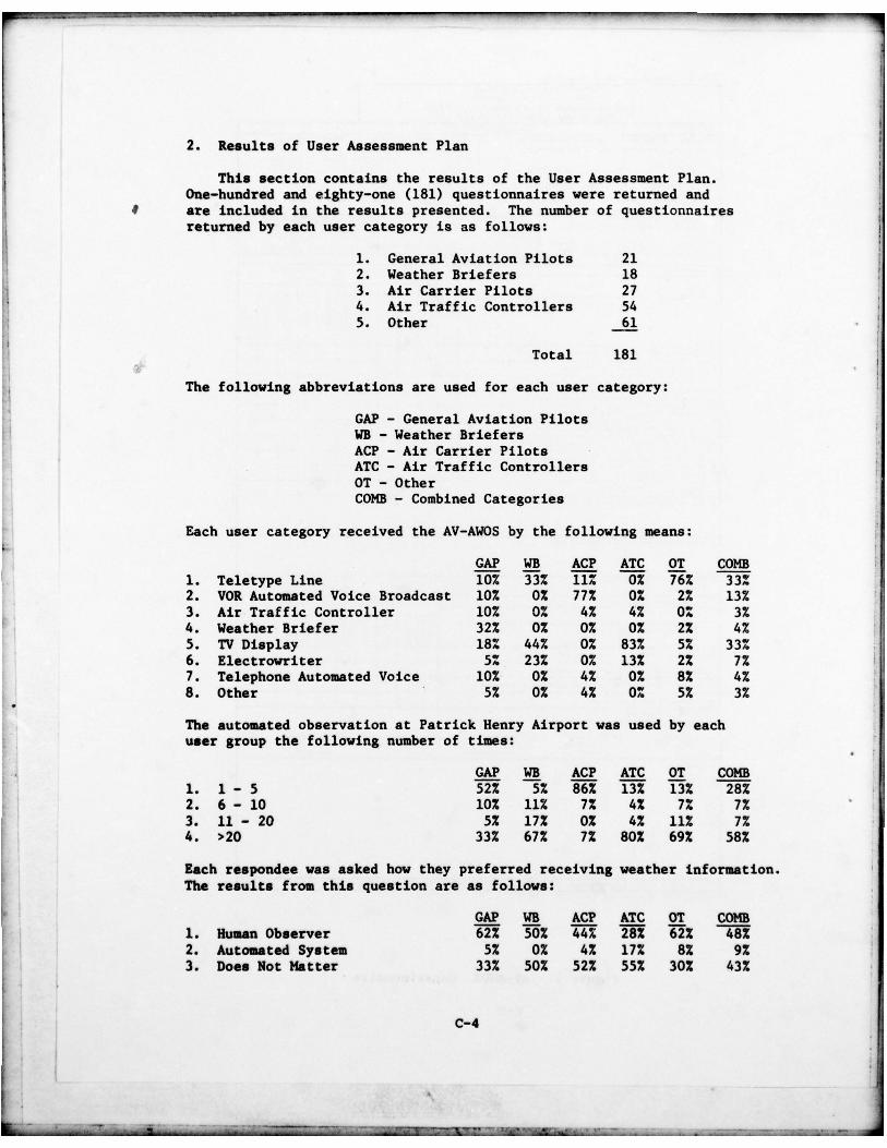
2. Results of User Assessment Plan
This section contains the results of the User Assessment Plan.One—hundred and eighty—one (181) questionnaires were returned andare included in the results presented. The number of questionnairesreturned by each user category is as follows:
1. General Aviation Pilots 212. Weather Briefers 183. Air Carrier Pilots 27
• 4. Air Traffic Controllers 545. Other 61
Total 181
The following abbreviations are used for each user category:
GAP — General Aviation PilotsWB — Wea ther BriefersACP — Air Carrier PilotsATC — Air Traff ic ControllersOT - OtherCOMB — Combined Categor ies -
•Each user category received the AV—AWOS by the following means:
GAP WB ACP ATC OT COMB1. Teletype Line 10% 33% 11% 0% 76% 33%2. VOR Automated Voice Broadcast 10% 0% 77% 0% 2% 13%3. Air Traffic Controller 10% 0% 4% 4% 0% 3%4. Weather Briefer 32% 0% 0% 0% 2% 4%5. TV Display 18% 44% 0% 83% 5% 33%6. Electrowriter 5% 23% 0% 13% 2% 7%7. Telephone Automated Voice 10% 0% 4% 0% 8% 4%8. Other
• 5% 0% 4% 0% 5% 3%
The automated observation at Patrick Henry Airport was used by eachuser group the following number of times:
- . GAP WB ACP ATC OT COMB1. 1 — 5 52% 5% 86% 13% 13% 28%
2. 6 — 10 10% 11% 7% 4% 7% 7%3. 11 — 20 5% 17% 0% 4% 11% 7%4. >20 33% 67% 7% 80% 69% 58%
Each respondee was asked how they preferred receiving weather information.The results from this question are as follows:
GAP WB ACP ATC OT COMB1. Human Observer 62% 50% 44% 28% 62% 48%2. Automated System 5% 0% 4% 17% 8% 9%3. Does Not Matter 33% 50% 52% 55% 30% 43%
C-4
- • —~~~~~~~~_ _
~~~~~~~~~~~~ •~~~~~• - -n--- .-- - ~~~~~~~~~~~~~~~~~~~~~ ~~~~~~~~~~~—‘- --~~~~~~ •- - ~~~~~~~~
- ~~~~~~~~~~~
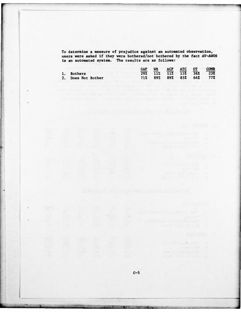
To determine a measure of prejudice against an automated observation,users were asked if they were bothered/not bothered by the fact AV—AWOSis an automated system. The results are as follows:
GAP WE ACP ATC OT COMB1. Bothers 29% 11% 11% 15% 36% 23%2. Does Not Bother 71% 89% 89% 85% 64% 77%
~~~~ ~~~~~~~~~~~~~~~~~~~~~~~~~~~~~~~~~~~~~~~~~~~ ~~~~~~~~~~~~~~~~~~~~~~~~~~~~~~~~~~~~~~
- :
~~~~~ ~~~~~~~~~ ~~~~~~~~~~~~~~~~~~~~~~~~~~~~~~~~~~~~ - . 1~~~~~~

~~~~~ rv ~~~—u-u~ ,— —
-
The unique features of the AV—AWOS System were evaluated via the user’squestionnaire. These included the height limitation of 7,000 feetfor cloud observations; the availability of the automated observation
• on TV displays; visibilities greater than 8 miles reported as 8+; theprovision of providing weather by automated voice over the telephone;present weather descriinination limited to only precipitation, freezingrain, hail and thunderstorms; more frequent updating of the observation ;
- - remarks on thunderstorms do not include bearing and movement; availabilityof local weather inflight on VOR via automated voice; fewer remarksreported ; and the AV—AWOS system considered in its entirety. Users ratedthese features in terms of desirability , importance or not applicableto their function. Their response to this section of the questionnaireis given below.
Height Limit of 7,000 Feet for Cloud Observation
1. DESIRABILITYGAP WE ACP NrC OT COMB
a. Very Undesirable/Undesirable 33% 5O~ 33% 20% 57% 39%b. Neutral 43% 33% 41% 56% 31% 41%c. Desirable/Very Desirable 19% 11% 26% 22% 8% 17%d. N/A or Left Blank 5% 6% 0% 2% 4% 3%
2. IMPORTANCEGAP WE ACP ATC OT COMB
a. Very Small/Small 23% 39% 55% 22% 20% 28%b. Moderate 29% 39% 26% 52% 48% 43%c. Great/Very Great 29% 16% 15% 15% 28% 21%d. N/A or Left Blank 29% 6% 4% 11% 4% 8%
Provision of Weather Observations Via TV Displays
1. DESIRABILITYGAP WB ACP ATC OT COMB
a. Very Undesirable/Undesirable 0% 6% 4% 31% 5% 12%b. Neutral 52% 27% 4% 9¼ 13% 17%c. Desirable/Very Desirable 43% 27% 26% 60% 31% 40%d. N/A or Left Blank 5% 40% 66% 0% 51% 31%
2. IMPORTANCE21 COMB
a. Very Small/Small 29% 28% 4% 13% 18% 17%b. Moderate 33% 11% 10% 40% 16% 21%c. Great/Very Great 14% 17% 19% 48% 12% 24%d. N/A or Left Blank 24% 44% 67%
- 9% 54% 38%
C-6
~~~j~~~-
~~~~~~~~~~~~~~~~~~~~~~~ ~~~~~~~~~~~~~~ - - •—--- ~~~~T1..~~~. n - . -
- ~~• --- ---~~~~~~~~~~~~~~~~~~~~~~~~~~~~~~~~~

_____ — ~~ 1 -: :-1 - - - — - a..—n--~~~~~~~~~ -— —• -— -- _____________________
All Visibilities Greater Than Eight (8) Miles Reported as “8+”
1. DESIRABILITYGAP WE ACP ATC OT COMB
• a. Very Undesirable/Undesirable 15% 0% 10% 9% 18% 12%b. Neutral 52% 72% 48% 44¼ 52% 51%c. Desirable/Very Desirable 33% 17% 38% 41¼ 28% 33%d. N/A or Left Blank 0% 11% 4% 6% 2% 4%
2. IMPORTANCEGAP WB ACP ATC OT COMB
a. Very Small/Small 247. 44% 44% 35% 56% 44%b. Moderate 43% 28% 30% 37% 30% 33%c. Great/Very Great 14% 17% 19% 17% 13% 15%d. N/A or Left Blank 19% 11% 7% 11% 1% 8%
Provision of Weather by Automated Voice Over the Telephone
1. DESIRABILITYGAP WB ACP ATC OT COMB
a. Very Undesirable/Undesirable 23% 17% 4% 20% 10% 14%b. Neu tral 29% 17% 152 172 20% 19%c. Desirable/Very Desirable 43% 22% 22% 17% 21% 23%d. N/A or Left Blank 5% 44% 59% 46% 49% 44%
2. IMPORTANCEGAP WE ACP ATC OT COMB
a. Very Small/Small 28% 117, 15% 20% 18%b. Moderate 24% 28% 15% 22% 20% 21%c. Great/Very Great 29% 67. 11% 13% 11% 13%d. N/A or Left Blank • 23% 38% 63% 50% 49% 48%
No Rain/Snow Discrimination — Precipitation Reported for Both
1. DESIRAB ILITYGAP WE ACP ATC OT COMB
a. Very Undesirable/Undesirable 86% 83% 84% 92% 86%b. Neutral 4% 11% 7% 9% 5% 7%c. Desirable/Very Desirable 10% 0% 0% 5% 3% 4%d. N/A or Left Blank 0% 6% 11% 2% 0% 3%
2. IMPORTANCEGAP WE ACP ATC OT COMB
a. Very Small/Small 5% 11% 7% 7% 7% 7%b. Moderate 19% 17% 22% 26% 8% 18%c. Great/Very Great 57% 61% 52% 56% 85% 65%d. N/A or Left Blank 19% 11% 19% 11% 0% 10%
C-7
A-
Ai:.: ~~~~ —-• - --

- - • -~~~~~~~1
More Frequent Weather Observation Updates
1. DESIRABILITYGAP WE ACP ATC OT COMB
a. Very Undesirable/Undesirable 5% 28% 11% 19% 8% 137,b. Neutral 38% 11% 22% 35% 11% 23%c. Desirable/Very Desirable 52% 50% 63% 46% ‘6% 60%d. N/A or Left Blank 5% 11% 4% 0% 5% 4%
2. IMPORTANCEGAP WE ACP ATC OT COMB
a. Very Small/Small 10% 22% 7% 15% 8% 12%b. Moderate 24% 22% 15% 41% 18% 25%c. Great/Very Great 42% 39% 71% 33% 69% 52%d. N/A or Left Blank 24% 17% 7% 11% 5% 11%
Remarks on Thunderstorms Do Not Include Bearing and Movement
1. DESIRABILITYGAP WE ACP ATC OT COMB
a. Very Undesirable/Undesirable 67% 44% 70% 51% 74% 627.b. Neutral 19% 33% 11% 20% 16% 19%c. Desirable/Very Desirable 10% 6% 11% 22% 5% 12%d. N/A or Left Blank 4% 17% 8% 7% 5% 7%
2. IMPORTANCEGAP WE ACP ATC OT COMB
a. Very Small/Small 0% 17% 7% 13% 11% 10%b. Moderate 19% 44% 26% 33% 21% 28%c. Great/Very Great 62% 28% 56% 39% 63% 51%d. N/A or Left Blank 19% 11% 11% 15% 5% 11%
• Availability of Local Weather Inf light via VOR Automated Voice
1. DESIRABILITYGAP WE ACP NrC OT COMB
a. Very Undesirable/Undesirable 02 5% 7% 7% 3% 5%b. Neutral 38% 5% 4% 20% 8% 14%c. Desirable/Very Desirable 57% 33% 82% 42% 23% 42%d. N/A or Left Blank 5% 57% 7% 31% 66% 39%
2. IMPORTANCEGAP WE ACP ATC OT COMB
a. Very Small/Small 17% 17% 0% 6% lOX 9%b. Moderate 10% 17% 26% 332 7% 19%c. Great/Very Great 49% 172 63% 24% 16% 29%d. N/A or Left Blank 24% 49% 11% 37% 67% 43%
c-8
_ _ _ _ _

- ~~~~~~~
—.- -~~~~ - - - - - ~~
__•__ _ _ _ __••7
~~_ .— -_—- —--- - —---- •— -~~~~~
Fewer Remarks Reported
1. DESIRABILITYGAP WB ACP ATC 01 COMB
a. Very Undesirable/Undesirable 38% 33% 41% 372 59% ~~ib. Neutral 47% 39% 33% 43% 31% 38%c. Desirable/Very Desirable 5% 11% 7% 13% 7% 9%d. N/A or Left Blank 10% 17% 19% 7% 3% 9%
2. IMPORTANCE
~~~ ~Ia. Very Small/Small 23% 33% 15% 28% 23% 24%b. Moderate 29% 28% 44% 33. 39% 36%c. Great/Very Great 19~
’L 22% 15% 22% 35% 25%d. N/A or Left Blank 29% 17% 26% 17% 3% 15%
AV—AWO S Considered in its Entirety
1. DESIRABILITYGAP WE ACP ATC OT COMB
a. Very Undesirable/Undesirable 23% l7~ 4% 31% 41% 28~b. Neutral 38% 22% 19% 20% 26% 24%c. Desirable/Very Desirable 29% 44% 67% 45% 30% 41%d. N/A or Left Blank 10% 17% 10% 4% 3% 7%
2. IMPORTANCEGAP WE ACP ATC OT COMB
a. Very Small/Small 28% 17% 0% 12% 167. 14%b. Moderate 24% 39% 62% 30% 43% 39%c. Great/Very Great 24% 22% 19% 41% 36% 33%d. N/A or Left Blank 24% 22% 197. 17% 5% 14%
Users were next asked to list the most desirable feature and the leastdesirable feature of AV—AWOS. The most frequent desirable features givenwere:
Frequent UpdateAutomated VoiceCloud and Visibility Observations
Fifty—six (56) percent of the respondees gave the frequent updatecapability of AV—AWOS as the most desirable feature.
C-9

_ _ _ _ _ _ ----~~--- - - -- - -~~~ - - - - - - - - - -~~------—-- -- - - --- -- --- - - - — - _ - - - -~~ ---~ -- •~~~~~~~
The most freq uent least desirable features given were :
Precipi tation Type LimitationAV-AWOS System Downt imeAutomated Voice Intelligibility
Forty—one (41) percent of the respondees gave the limitation ofthe AV— AM~~S in reporting precipitation types as the least desirablefeature.
Only fifty—five (55) users gave their evaluation of the automatedvoice capability of AV—AWOS. Instead of listing the response byuser category , the responses were combined for all categories.
Telephone
1. INTELLIGIBILITY, DISTORTION, NOISE, FIDELITY
a. Very Poor/Poor 182b. Fair 29%c. Good/Very Good 532
2. SUITABILITY OF SPEAKING RATE
a. Very Poor/Poor 6%b . Fair 232c. Good/Very Good
3. NATURALNESS OF RHY THM, SMOOTIINES!
a. Very Poor/Poor 212b. Fair 24%c. Good/Very Good 552
4. OVERALL PLEASANTNESS
a. Very Poor/Poor 212b . Fair 36%c. Good/Very Good 432
c-b
- ~~~~~~~~~~~~~~~~~~~~~~~~~~~ - • •
- • ~~~~~~~~~~~ ~~~~~~~~~~~~~~~~~~~~~~~~~~~~~~~~~~~ - -- ~~~~-~~~~~_____

VOR (VH F Omni Range)
1. INTELLIGIBILITY, DISTORTION, NOISE, FIDELITY
a. Very Poor/Poor 30%b. Fair 40%c. Good/Very Good 30%
2. SUITABILITY OF SPEAKING RATE
a. Very Poor/Poor 7%b. Fair 16%c. Good/Very Good 77%
3. NA TURALNESS OF RHYTHM, SMOOTHNESS
a. Very Poor/Poor 23%b. Fair 23%c. Good /Very Good 54%
4. OVERALL PLEASANTNESS
a. Very Poor/Poor 24%b. Fair 30%c. Good/Very Good 46%
The overall suitability of AV—AWOS for widespread field use was rated byusers of the automated observation. The results by user category are asfollows:
1. SUITABLE, FINE AS IS
a. General Aviation Pilots 0%b. Weather Briefers 0%c. Air Carrier Pilots 0%d. Air Traffic Controllers 2%e. Other 2%f . Combined < 1%
2. SUITABLE, MINOR CHANGES DESIRABLE
a. General Aviation Pilots 55%b. Weather Briefers 33%c. Air Carrier Pilots 63%d. Air Traffic Controllers 46%e. Other 26%f . Combined 42%
C—lb
I:- ~~~-- -~~~ -~~ ---- — ___
— —•---- - - ~~~~~~~~~ ~~~~~~~~~~~~~~~~~~~~~~~ ~~~~~~~~~~~~~~~~~~~~~~~~~ -

~~~~ --— —- -- -~~
3. MARGINALLY SUITABLE, MAJOR CHANGES NECESSARY
a. General Aviation Pilots 25%b. Weather Briefers 61%c. Air Carrier Pilots 33%d. Air Traffic Controllers 33%e. Other
.
f . Combined 39%
4. UNSUITABLE, EXTENSIVE REDESIGN
a. General Aviation Pilots 5%b. Weather Brief ers OXc. Air Carrier Pilots 4%d. Air Traffic Controllers 13%e. Other 11%f . Combined 9%
5. UNSUITABLE, ENTIRE CONCEPT IS INAPPROPRIATE
a. General Aviation Pilots 15%b. Weather Briefers 6%c. Air Carrier Pilots 02d. Air Traff ic Controllers 6%e. Other 18%f . Combined 10%
C—1 2
~~~~~~ ~~~~~~~~~~~~~~~~~~~~~~~~~~~~~~~~~~~~~~~~~~~~~~~ - ~~ ~~~~~~~~- : __~~~~~
-. ~~~~~~~~~~~~ L.~~ :•~~~ L -~~~~
-~~
-~~-
-- — -- - - ----- . ~~~~~~~~~~~~~ ~~~~~~~~~~~