Approximations to the Stochastic Burgers Equation

Martin Hairer, Jochen Voss

24th May 2010

Abstract

This article is devoted to the numerical study of various finite difference approximationsto the stochastic Burgers equation. Of particular interest in the one-dimensional case isthe situation where the driving noise is white both in space and in time. We demonstratethat in this case, different finite difference schemes converge to different limiting processesas the mesh size tends to zero. A theoretical explanation of this phenomenon is given andwe formulate a number of conjectures for more general classes of equations, supported bynumerical evidence.

Keywords: stochastic Burgers equation, correction term, numerical approximationSubject classification: 60H35, 60H15, 35K55

1 Introduction

This article studies several finite difference schemes for the viscous stochastic Burgers equation:

∂tu(x, t) = ν ∂2xu− g(u) ∂xu+ σ ξ(x, t), x ∈ [0, 2π], t ≥ 0. (1)

In this equation, ξ denotes space-time white noise, that is the centred, distribution-valued Gaus-sian random variable such that E

(ξ(x, t)ξ(y, s)

)= δ(t − s)δ(x − y). We will always endow this

equation with periodic boundary conditions and we will consider solutions u taking values eitherin R or in Rn (in which case g is matrix-valued in general).

Motivations for studying the stochastic Burgers equation are manifold. Just to name a few,it is used to model vortex lines in high-temperature superconductors [BFG+94], dislocations indisordered solids and kinetic roughening of interfaces in epitaxial growth [Bar96], formation oflarge-scale structures in the universe [GSS85, SZ89], constructive quantum field theory [BCJL94],etc. Since in the case σ = 0 and g(u) ∝ u this equation is furthermore explicitly solvable viathe Hopf-Cole transform (u = ∂xv/v, where v solves the heat equation), it comes as no surprisethat a wealth of numerical and analytical results are available. From a purely mathematicalpoint of view, let us mention for example the well-posedness results from [BCF91, BCJL94,DPDT94, Gyo98, Kim06] and the ergodicity results obtained in [TZ06, GM05]. One remarkableachievement was the construction of a stationary solution in the inviscid limit with non-vanishingnoise [EKMS00] (dissipation then occurs purely through shocks). From a more quantitativeperspective, the scaling exponents of the solutions in the small viscosity limit have attractedconsiderable interest, both in the physics and the applied mathematics literature [YC96, BM96,Kra99, EVE00a, EVE00b].

The white noise term ξ in (1) leads to solutions u which, in general, will be very “rough”.In particular, u as a function of the spatial variable x will not be differentiable in the classicalsense, but will only possess some Holder regularity. As a consequence, it transpires that thesolutions to (1) are extremely unstable under natural approximations of the nonlinearity, andthis is the phenomenon that will be explored in this article. For example, for any a, b ≥ 0 witha+ b > 0, one can consider the approximating equation

∂tuε(x, t) = ν ∂2xu

ε − g(uε)Dεuε(x, t) + σ ξ(x, t), (2)

where the approximate derivative Dε is defined as

Dεu(x, t) =u(x+ aε, t)− u(x− bε, t)

(a+ b)ε. (3)

1

In the absence of the noise term ξ it would be a standard exercise in numerical analysis to showthat the solution of (2) converges to the solution of (1) as ε→ 0. This is just an example of thewidely accepted ‘folklore’ fact that, if an equation is well-posed, any ‘reasonable’ approximationwill converge to the exact solution.1

In this article, we will argue that, if ξ is taken to be space-time white noise, the limit of(2) as ε → 0 depends on the values a and b and is equal to (1) only if either g is constant ora = b! Furthermore, it will follow from the argument that, if one considers driving noise that isslightly rougher than space-time white noise (taking a noise term equal to (1− ∂2x)α dw(t) withα ∈ (0, 1/4) still yields a well-posed equation), one does not expect solutions to the approximateequation (2) to converge to anything at all, unless a = b. Our methodology here is to firstpresent a heuristic argument which allows to derive quantitative predictions for the effect of thefinite difference discretisation on the solution. We will then use numerical experiments to verifythese predictions.

At this point we would like to emphasise that the aim of this article is certainly not toadvocate the use of a finite difference scheme of the type (2) to effectively simulate (1). Indeed,we will show in section 2.2 below that approximations of the nonlinearity of the type DεG(u),where G is the antiderivative of g already have much better stability properties. Instead, ouraim is merely to give a striking illustration of the fact that caution should be exercised in thesimulation of stochastic PDEs driven by spatially rough noise.

The text is structured as follows: We start in section 2 by presenting our argument for thecase of the stochastic Burgers equation, i.e. for g(u) = u. In section 3 we will present thecorresponding results for more general equations and in section 4 we study the limit of vanishingnoise and viscosity. Finally, in appendix A we discuss some technical aspects of the simulationsused throughout this article.

Acknowledgements

We would like to thank Andrew Majda, Andrew Stuart, Eric Vanden Eijnden, and Sam Fallefor helpful discussions of the phenomena discussed in this article. Financial support was kindlyprovided by the EPSRC through grants EP/E002269/1 and EP/D071593/1, as well as by theRoyal Society through a Wolfson Research Merit Award. JV would like to thank the CourantInstitute, where work on this article was started, for its hospitality.

2 Stochastic Burgers Equation

In this section we consider the stochastic Burgers equation

du = ν ∂2xu dt− u ∂xu dt+ σ dw, (4)

as well as the approximation given by

duε = ν ∂2xuε dt− uεDεu

ε dt+ σ dw. (5)

The solutions u and uε take values in the space L2([0, 2π],R

)on which the operator ∂2x is

endowed with periodic boundary conditions, and w is an L2-cylindrical Wiener process (see[DPZ92] for details). Equation (4) is well-posed, since we can rewrite u ∂xu as 1

2∂x(u2) which

is locally Lipschitz from the Sobolev space H1/4 into H−1, thus allowing us to apply generallocal well-posedness theorems as in [DPZ92, Hai09]. For fixed time t > 0, the solutions to (4)have the regularity of Brownian motion when viewed as a function of the spatial variable x. Inparticular, they are not differentiable in x. Figure 1 shows numerical solutions of equation (5)for different values of a and b. One can see that different choices for these parameters lead toan O(1) difference in the solutions.

Our aim in this article is to understand and quantify these differences. In particular, inconjecture 1 below, we compute a correction term to (4) and we verify numerically that thesolutions to (5) converge to the corrected equation as ε→ 0. This understanding will then allowus to conjecture the appearance of similar correction terms in more complicated situations andwe will again verify these conjectures numerically.

1Remember that we are working at fixed non-zero viscosity here, so there is no ambiguity in the concept ofsolution and we do not require an upwind scheme in order to obtain convergence.

2

0 1 2 3 4 5 6x

�6

�4

�2

0

2

4

6

ua,b(1,x

)

Figure 1: Illustration of the discretisation error for the finite difference method (5). The threelines correspond to a right-sided discretisation (a = 1, b = 0; top-most curve), a centred discreti-sation (a = 1, b = 1; middle curve) and a left-sided discretisation (a = 0, b = 1; bottom-mostcurve), all computed using the same instance of the driving noise. The picture clearly shows thatthere is an O(1) difference between the solutions obtained by the three different discretisationschemes. From the argument presented in the text, we assume that the exact solution of (4) willbe closest to the middle of the three lines.

2.1 Heuristic Explanation

For simplicity, instead of u we consider the solution v to the stochastic heat equation

dv = ν ∂2xv dt+ σ dw(t). (6)

Since the properties of the discretisation of differential operators only depend on local properties,and since v has the same spatial regularity as u, it will be sufficient to study how well v Dεvapproximates v ∂xv = 1

2∂xv2.

By expressing v in the Fourier basis{

einx/√

2π}n∈Z it is easy to check that the stationary

solution to (6) is

v(t, x) =∑

n∈Z\{0}

σ

in√

2νξn(t)

einx√2π

+ ξ0(t)1√2π,

where the ξ0 is a (real-valued) standard Brownian motion and ξn for n 6= 0 are complex-valuedOrnstein-Uhlenbeck processes with variance 1 (in the sense that E|ξn(t)|2 = 1) and time constantνn2 which are independent, except for the condition that ξ−n = ξn. Therefore, the derivative ofv is given (at least formally) by

∂xv(x) =∑n 6=0

σξn(t)einx

2√νπ

. (7)

The ε-approximation to the derivative given in (3), on the other hand, is given by

Dεv(x) =∑n 6=0

σξn(t)einx

2√νπ

einaε − e−inbε

(a+ b)iεn. (8)

It is clear that the terms in (8) are a good approximation to the terms in (7) only up to n ≈ ε−1.For larger n, the multiplier in (8) will decrease like n−1.

For our analysis we restrict ourselves to the constant (n = 0) Fourier mode. Our numericalexperiments, below, show that the contributions from this mode are already enough to explainthe observed differences between the solutions of the approximating equation (5) and the exact

3

solution. Since v ∂xv is a total derivative, the 0-mode of this term vanishes. In contrast, the0-mode of v Dεv does not vanish at all: We obtain instead for this term the sum

⟨vDεv

∣∣ 1√2π

⟩=

1√2π

∑n6=0

σ2ξ−n(t)ξn(t)

2ν(−in)

einaε − e−inbε

(a+ b)εin

=σ2

√2πν

∑n>0

|ξn(t)|2 cos aεn− cos bεn

(a+ b)εn2

(9)

and the expectation of this expression, as ε→ 0, converges to

limε↓0

E(−vDεv

)(x) = lim

ε↓0E⟨−vDεv

∣∣ 1√2π

⟩ 1√2π

= − σ2

2πν

∫ ∞0

cos aκ− cos bκ

(a+ b)κ2dκ =

σ2

4ν

a− ba+ b

.

As a consequence, one expects the following result.

Conjecture 1 The solution of the approximating equation (5) converges, as ε → 0, to thesolution of

du = ν ∂2xu dt− u ∂xu dt+σ2

4ν

a− ba+ b

dt+ σ dw. (10)

Thus, the approximation converges to the stochastic Burgers equation (4) only for a = b.

Remark 2.1 The solution to the stochastic Burgers equation (or rather the integrated processwhich solves the corresponding KPZ equation) arising as the fluctuations process in the weaklyasymmetric exclusion process [BG97, BQS09] is driven by the derivative of space-time whitenoise. As a consequence, it does not solve an SPDE that is well-posed in the classical sense andcan currently only be defined via the Hopf-Cole transform. Such a process is even rougher (by“one derivative”) than the process considered here and one would expect the ‘wrong’ numericalapproximation schemes to fail there in an even more spectacular way.

Remark 2.2 One may think of two reasons why the correction term vanishes when a = b. Onthe one hand, this discretisation is more symmetric. On the other hand, it yields a second-orderapproximation to the derivative at x. The correct explanation is closer to the first one. Indeed,consider for example the discretisation(

Dεu)(x) ≈ c u(x+ 2ε) + (1− 3c)u(x+ ε) + 3c u(x)− (1 + c)u(x− ε)

2ε. (11)

This discretisation is of second order for every c ∈ R. However, if we perform the same calculationas above with this discretisation, we obtain a correction term equal to

σ2

2πν

∫ ∞0

c cos 2κ− 4c cosκ+ 3c

2κ2dκ = −cσ

2

8ν,

which vanishes only if c = 0, i.e. when (11) conincides with the symmetric discretisation (3).

In the above calculation, both the limiting equation and the approximating equation live inthe same space. It is possible to carry out a similar analysis in the case where the approximatingequation takes values in a different space, typically RN for some large N . For example, we canconsider the ‘finite difference’ approximation given by

∂2xu ≈u(x+ δ)− 2u(x) + u(x− δ)

δ2def=(∆Nu

)(x)

u ∂xu ≈ uDδu = u(x)u(x+ δ)− u(x)

δ

def= FN (u)(x),

(12)

where we set δ = 2πN for the approximation with N gridpoints. In this setting, we approximate

u by uN ∈ RN with uNj ≈ u(jδ). The natural candidate for the approximation of space-time

4

white noise is then given by dWNj = δ−1/2 dWj , where the Wj are independent, one-dimensional

standard Brownian motions. This is the correct scaling, since it ensures for example that for everycontinuous function g,

∑jW

Nj g(δj) is a Wiener process with covariance

∑j g(δj)2δ ≈

∫g2 dx.

With this notation, we consider the approximating equation given by

duN = ν∆NuN dt− FN (uN ) dt+ σ dWN (t). (13)

Let us take N even for the sake of simplicity. It is then straightforward to check that theeigenvectors for ∆N are given as before by einx with n = −N2 + 1, . . . , N2 , but the correspondingeigenvalues are

λn =2

δ2(cosnδ − 1

)= −

(2

δsin(nδ

2

))2 def= −η2n.

(Note that for fixed n and small δ, one has indeed λn ≈ −n2.) It then follows as previously thatthe solution to the linearised equation is given by

v(t, x) =∑n 6=0

σ

2√νπiηn

einxξn(t) + ξ0(t)1√2π

and that its discrete derivative Dδv is given by

Dδv(t, x) =∑n 6=0

σeinxξn(t)

2√νπiηn

einδ − 1

δ.

Note that the sums in both expressions only run over the values n = −N2 + 1, . . . , N2 . Similarlyto above, we obtain that the expectation of the zero mode of the product v Dδv is given by

E⟨−vDεv

∣∣ 1√2π

⟩ 1√2π

= − σ2

2πν

N/2∑n=1

cos δn− 1

δη2n=

σ2

2πν

N/2∑n=1

δ

2=σ2

4ν. (14)

One therefore expects the following result.

Conjecture 2 The solution uN of the finite difference approximation (13) converges, as N →∞, to the solution of

du = ν ∂2xu dt− u ∂xu dt+σ2

4νdt+ σ dw(t).

To test this conjecture, we use the following numerical experiment: We numerically solveboth the “approximating” equation (13) and the “corrected” SPDE

duγ = ν ∂2xuγ dt− uγ ∂xuγ dt+ γσ2

νdt+ σ dw(t), (15)

until a fixed time T , using the same instance of the noise. To discretise the term u ∂xu in (15)we use the approximation

(u(x)2/2 − u(x − δ)2/2

)/δ, which is known to converge to the exact

solution, see section 2.2 below. Also, for increased accuracy, we use a finer grid for (15) thanwe did for (13). Now we can compare the two solutions by considering ‖uN (T, · ) − uγ(T, · )‖2as a function of γ: If conjecture 2 is correct, this function will take its minimum at γ ≈ 1/4.The result of such a simulation is given by the line labelled “finite difference” in figure 2. Theminimum of the curve is indeed located close to γ = 1/4, thus giving support to conjecture 2.

Even though the correction terms in conjectures 1 and 2 (with a = 1 and b = 0) coincide, theconstants arise in completely different ways. This might lead to the speculation that the value ofthis constant is an intrinsic property of the limiting equation, rather than of the particular wayof approximating it. The following argument shows that this is not the case. One can repeat thecalculation leading to conjecture 2 with a ‘spectral Galerkin’ approximation of the linear part ofthe equation, but retaining a ‘finite difference’ approximation of the nonlinearity. In other words,we consider (13) as before, but we take for ∆N the self-adjoint matrix with eigenvectors einx andeigenvalues −n2. (This can be achieved by first applying the discrete Fourier transform, then

5

0.0 0.1 0.2 0.3 0.4 0.5�

0

1

2

3

4

5

6

7

8

||uN

(1,·)

�

u�

(1,·)

|| 2

finite difference Galerkin

Figure 2: This figure compares the solution uN of the finite difference approximation (13) to thesolution uγ of the “corrected” SPDE (15) (which includes an additional drift term γσ2/ν). Thecurves show the L2-norm difference between the solutions (for the same instance of the noise) asa function of γ, once using finite difference discretisation (12) of the linear part (correspondingto the top-most curve in figure 1) and once using the spectral Galerkin discretisation. The twovertical line segments give the predicted locations for the minima of the two curves. It can beseen that predictions and simulations are in good agreement.

multiplying the nth component by −n2, and finally applying the inverse Fourier transform.) Inthis case one has ηn = n and it transpires that the correction term is given by

N/2∑n=1

σ2

2πνη2n

1− cosnδ

δ≈ σ2

2πν

∫ π

0

1− cosκ

κ2dκ ≈ 0.193σ2

ν.

which is clearly different from (14).To verify that the spectral Galerkin discretisation of the linear part indeed leads to this

different correction term, we modify the code which we used to validate conjecture 2 above. Theresult of this simulation is given by the line labelled “Galerkin” in figure 2. Again, there is goodagreement between our conjecture and the simulation results.

2.2 The Case of More Regular Noise

To conclude this section, let us argue that the situation considered in this article is truly aborderline case in terms of regularity and that if we drive (5) by noise that gives rise to slightlymore regular solutions, the solutions of (5) converge to those of (4) without any correction term.Indeed, consider a general semilinear stochastic PDE driven by additive noise:

du = −Audt+ F (u) dt+Qdw(t), (16)

where A is a strictly positive-definite selfadjoint operator on some Hilbert space H, F is a(possibly unbounded) nonlinear operator from H to H, W is a standard cylindrical Wienerprocess on H, and Q : H → H is a bounded operator.

Denote furthermore Hα = D(Aα) for α > 0 and let H−α be the dual space to Hα under thedual pairing given by the Hilbert space structure of H. (So that H−α is a superspace of H forα > 0.) We also denote by ‖ · ‖α the natural norm of Hα. Finally, we denote as before by v thesolution to the linearised system

dv = −Av dt+Qdw(t),

which we assume to be an H-valued Gaussian process with almost surely continuous samplepaths. One then has the following convergence result:

6

Theorem 2.3 Assume that there exists γ ≥ 0 and a ∈ [0, 1) such that F : Hγ → Hγ−a is locallyLipschitz continuous and such that the process v has continuous sample paths with values in Hγ .Assume furthermore that Fε : Hγ → Hγ−a is such that Fε is locally Lipschitz and such that theconvergence Fε(u)→ F (u) takes place in Hγ−a, locally uniformly in Hγ . Then, the solutions uεto

duε = −Auε dt+ F (uε) dt+Qdw(t), (17)

converge to the solutions to (16) as ε→ 0.

Proof. The proof is straightforward and we only sketch it. We assume without loss of generalitythat the parameter ε is chosen in such a way that for every R > 0 there exists a constant CRsuch that

sup‖x‖γ≤R

‖Fε(u)− F (u)‖γ−a ≤ CRε. (18)

Denote now by u the solution to (16) with initial condition u0 and by uε the solution to (17) withinitial condition uε0. Let t > 0 be small enough so that ‖u(s)‖γ ≤ R and ‖u(s) − uε(s)‖γ ≤ Rfor s ≤ t. We then have

‖u(t)− uε(t)‖γ ≤ ‖u0 − uε0‖γ + C

∫ t

0

(t− s)−a‖Fε(uε(s))− F (u(s))‖γ−a ds

≤ ‖u0 − uε0‖γ + C

∫ t

0

(t− s)−a‖Fε(uε(s))− F (uε(s))‖γ−a ds

+ C

∫ t

0

(t− s)−a‖F (uε(s))− F (u(s))‖γ−a ds

≤ ‖u0 − uε0‖γ + CRε+ CRt1−a sup

s≤t‖u(s)− uε(s)‖γ .

The claim then follows by taking t sufficiently small and performing a simple iteration.

Despite its simplicity, this criterion is surprisingly sharp. Indeed, we argue that if we consider(4) but with the space-time white noise dw replaced by (1 − ∂2x)−δ dw for δ > 0, then theassumptions of theorem 2.3 can be satisfied with some choice of exponent γ for the approximation

Fε(u)(x) = u(x)u(x+ ε)− u(x)

ε

def= u(x)

(Dεu

)(x).

Obviously, this cannot be the case when δ = 0, since we then observe the convergence to solutionsto (10).

Indeed, we first note that since the linear operator appearing in (4) is of second order, wehave the correspondence

Hγ = H2γ ,

between interpolation spaces and fractional Sobolev spaces. In order to keep our notation coher-ent throughout this section, we still denote by ‖ · ‖γ the norm of Hγ , i.e. ‖u‖γ = ‖(1−∂2x)γu‖L2 ,where we implicitly endow ∂2x with periodic boundary conditions. With this notation, we getthe following result.

Lemma 2.4 For γ ≥ 0 and a ∈ [ 12 , 1], we have ‖Dεu− ∂xu‖γ−a ≤ Cε2a−1‖u‖γ .

Proof. The operator Dε−∂x is given by the Fourier multiplier Mε(k) = ε−1(eikε− 1− ikε

). We

immediately obtain the bound

|Mε(k)| ≤ k(εk ∧ 1

)≤ k(εk)2a−1,

from which the claim follows at once.

Since furthermore Hγ is an algebra for γ > 14 , we conclude that the bound (18) holds (for

some different power of ε), provided that we choose γ ∈ ( 14 ,

12 ] and a = 2γ. On the other hand,

the solution to the linearised equation

dv = ∂2xv dt+ (1− ∂2x)−δ dw

7

0.0 0.2t

05

10152025303540

||ua,b(t,·)

|| 2

�=�1/4

0.2 0.4t

�=�1/8

0.2 0.4 0.6 0.8t

�=�1/16

a=1, b=1

a=1, b=0

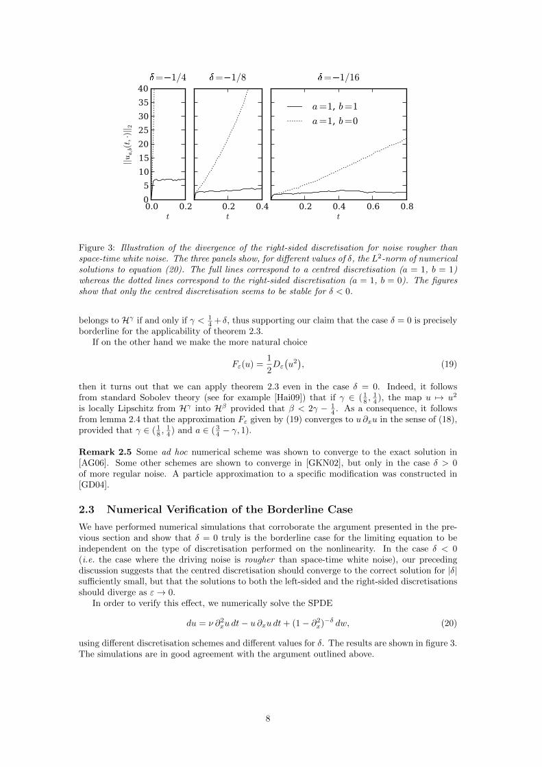
Figure 3: Illustration of the divergence of the right-sided discretisation for noise rougher thanspace-time white noise. The three panels show, for different values of δ, the L2-norm of numericalsolutions to equation (20). The full lines correspond to a centred discretisation (a = 1, b = 1)whereas the dotted lines correspond to the right-sided discretisation (a = 1, b = 0). The figuresshow that only the centred discretisation seems to be stable for δ < 0.

belongs to Hγ if and only if γ < 14 + δ, thus supporting our claim that the case δ = 0 is precisely

borderline for the applicability of theorem 2.3.If on the other hand we make the more natural choice

Fε(u) =1

2Dε

(u2), (19)

then it turns out that we can apply theorem 2.3 even in the case δ = 0. Indeed, it followsfrom standard Sobolev theory (see for example [Hai09]) that if γ ∈ ( 1

8 ,14 ), the map u 7→ u2

is locally Lipschitz from Hγ into Hβ provided that β < 2γ − 14 . As a consequence, it follows

from lemma 2.4 that the approximation Fε given by (19) converges to u ∂xu in the sense of (18),provided that γ ∈ ( 1

8 ,14 ) and a ∈ ( 3

4 − γ, 1).

Remark 2.5 Some ad hoc numerical scheme was shown to converge to the exact solution in[AG06]. Some other schemes are shown to converge in [GKN02], but only in the case δ > 0of more regular noise. A particle approximation to a specific modification was constructed in[GD04].

2.3 Numerical Verification of the Borderline Case

We have performed numerical simulations that corroborate the argument presented in the pre-vious section and show that δ = 0 truly is the borderline case for the limiting equation to beindependent on the type of discretisation performed on the nonlinearity. In the case δ < 0(i.e. the case where the driving noise is rougher than space-time white noise), our precedingdiscussion suggests that the centred discretisation should converge to the correct solution for |δ|sufficiently small, but that the solutions to both the left-sided and the right-sided discretisationsshould diverge as ε→ 0.

In order to verify this effect, we numerically solve the SPDE

du = ν ∂2xu dt− u ∂xu dt+ (1− ∂2x)−δ dw, (20)

using different discretisation schemes and different values for δ. The results are shown in figure 3.The simulations are in good agreement with the argument outlined above.

8

3 Possible Generalisations of the Argument

In this section, we discuss a number of possible extensions of these results to more generalBurgers-type equations. We restrict ourselves in this discussion to the case a = 1, b = 0, i.e.to right-sided discretisations. This is purely for notational convenience, and one would expectsimilar correction terms to appear for arbitrary values of a and b, just as before.

3.1 More General Nonlinearities

Consider the equation

dui = ν ∂2xui dt+

d∑j=1

∂jhi(u)∂xuj dt+ σ dwi, (21)

for an Rd-valued process u and a smooth function h : Rd → Rd with bounded second and thirdderivatives. Rewriting the nonlinearity as ∂x

(hi(u)

), we see that this equation is globally well-

posed. As before, we consider the approximating equation

duεi (x, t) = ν ∂2xuεi (x, t) dt+

d∑j=1

∂jhi(uε(x, t)

)Dεu

εj(x, t) dt+ σ dwi(t). (22)

The idea now is to introduce a cut-off frequency N and to write uε = uε + uε, where uε isthe projection of uε onto Fourier modes with |k| ≤ N . Since the linear part of the equationdominates the nonlinearity at high frequencies, one expects uε to be well approximated by v,the projection of v onto the high frequencies. This on the other hand is small in the L∞ norm(it decreases like N−s for every s < 1

2 ), so that

∂jhi(uε) ≈ ∂jhi(uε) +

d∑k=1

∂2jkhi(uε)vk.

It now follows from the same argument as before that the term ∂2jkhi(uε)vkDεvj is expected to

yield a non-vanishing contribution for k = j in the limit ε→ 0 and N →∞. Provided that wekeep N � 1

ε , this contribution will again be described by (9), so that we expect the followingbehaviour:

Conjecture 3 The solution of (22) converges, as ε→ 0, to the solution of

dui = ν ∂2xui dt+∑j

(∂jhi(u)∂xuj −

σ2

4ν∂2jjhi(u)

)dt+ σ dwi. (23)

In the one-dimensional case we can recover conjecture 1 (for a = 1, b = 0) from conjecture 3by choosing h(u) = −u2/2 in (23).

We perform the following numerical experiment to validate the functional form of the correc-tion term given in conjecture 3: We numerically solve both the “approximating” equation (22)and, for p : R→ R, the “corrected” SPDE

dup = ν ∂2xup dt+ h′(up)∂xup dt−σ2

4νp(up) dt+ σ dw (24)

until a fixed time T , using the same instance of the noise. As for the discretisation of (15)above, we use the approximation

(h(x) − h(x − δ)

)/δ for the term h′(u) ∂xu in the proposed

limit (24) and we also solve (24) on a finer grid than we use for (22). Finally, we numericallyoptimise the correction term p (using some parametric form) in order to minimise the distance‖uN (T, · ) − up(T, · )‖2. If the conjecture is correct, we expect the minimum to be attained fora function p which is close to the predicted correction term h′′. The result of a simulation isshown in figure 4. The figure shows that there is indeed a good fit between the conjectured andnumerically determined correction terms.

9

�0.4

�0.2

0.0

0.2

0.4

p(u

)

�2 �1 0 1 2u

0.00.10.20.30.40.50.6

hist

ogra

m o

f uN

(0.1,·)

Figure 4: Illustration of the convergence of (22) to (23) for the one-dimensional example h′(x) =sin(x)2. For the figure we numerically compute the finite difference solution uN to (22). Wethen compute solutions up to (24), using a fifth-order polynomial for the correction term p. Thispolynomial is then numerically fitted to minimise ‖uN (1, · )−up(1, · )‖2. The top panel shows theresulting fitted correction term −σ2p/4ν (full line) together with the correction term −σ2h′′(u)/4νpredicted in conjecture 3 (dotted line). To give an idea which range of the correction term isactually used in the computation, the lower panel shows the histogram of the values of uN (thevertical bars indicate the 5% and 95% quantiles). Between these quantiles, the graph shows agood fit between the numerically determined and conjectured correction terms.

10

3.2 Classically Ill-Posed Equations

Pushing further the class of equations considered in the previous subsection, one may want toconsider equations of the form

dui = ν ∂2xui dt+

d∑j=1

Gij(u)∂xuj dt+ f(u) dt+ σ dwi (25)

for some functions G : Rd → Rd×d and f : Rd → Rd. If we do not assume that G has anantiderivative and since solutions are only expected to be α-Holder continuous in space forα < 1

2 , it is no longer even clear what it means to be a solution to this equation. So, at leastclassically, (25) is ill-posed and the mere concept of solutions to such an evolution equation isdifficult to establish.

However, the discretised equation does of course still make sense for any fixed value of ε.Furthermore, we observed numerically that there seems to be no instability as ε→ 0; indeed oneobserves pathwise convergence to a limiting process. By analogy with the behaviour observed forthe situations where (25) is classically well-posed (i.e. when G has an antiderivative), one wouldthen be tempted to define solutions to (25) to be those processes that can be obtained as limitsas ε→ 0 of the solutions to the equation where ∂xuj is replaced by its symmetric discretisation.In analogy with conjecture 3, we would then expect solutions of the right-sided discretisation toconverge, as ε→ 0, to solutions of the corrected equation

dui = ν ∂2xui dt+∑j

(Gij(u)∂xuj −

σ2

4ν∂jGij(u)

)dt+ f(u) dt+ σ dwi.

This reasoning leads to:

Conjecture 4 As ε→ 0, the equations

duεi = ν ∂2xuεi dt+

d∑j=1

Gij(uε)D1,0

ε uεj dt+ f(uε) dt+ σ dwi, (26)

where D1,0ε denotes the right-sided discretisation, and

duεi = ν ∂2xuεi dt+

d∑j=1

(Gij(u

ε)D1,1ε uεj −

σ2

4ν∂jGij(u

ε))dt+ f(uε) dt+ σ dwi, (27)

where D1,1ε denotes centred discretisation, converge to the same limit.

To test conjecture 4, we use the following numerical experiment: as an example we considerthe SPDE

∂tu =1

σ2∂2xu+

2

σ2

(0 cos(u2)− sin(u1)

sin(u1)− cos(u2) 0

)∂xu

+4

σ2

(sin(u1) cos(u1)− cos(u2) sin(u2)

)+√

2 ∂tw.

(28)

This SPDE is of the form (25) where G has no antiderivative. SPDEs like (28) occur in theproblem described in [HSV07, section 9] where we argue that the stationary distribution of thisSPDE on L2

([0, 2π],R2

)(when equipped with appropriate boundary conditions) coincides with

the distribution of the stochastic differential equation

dU(t) = 2

(− sin(U2(t))

cos(U1(t))

)dt+ σ dB(t).

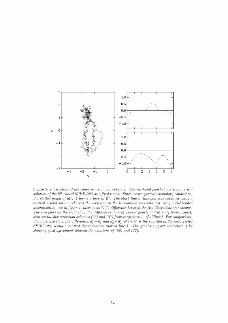
For our experiment we numerically solve the SPDEs (26) and (27) and compare the solutions.The result is displayed in figure 5. As can be seen from the figure, the simulation results are ingood agreement with conjecture 4.

11

�3 �2 �1 0u2

�3

�2

�1

0

1

2

3

u1

0 1 2 3 4 5 6t

�1.0

�0.5

0.0

0.5

1.0

�1.0

�0.5

0.0

0.5

1.0

Figure 5: Illustration of the convergence in conjecture 4. The left-hand panel shows a numericalsolution of the R2-valued SPDE (28) at a fixed time t. Since we use periodic boundary conditions,the plotted graph of u(t, · ) forms a loop in R2. The black line in this plot was obtained using acentred discretisation, whereas the grey line in the background was obtained using a right-sideddiscretisation. As in figure 1, there is an O(1) difference between the two discretisation schemes.The two plots on the right show the differences uε1 − uε1 (upper panel) and uε2 − uε2 (lower panel)between the discretisation schemes (26) and (27) from conjecture 4. (full lines). For comparison,the plots also show the differences uε1− uε1 and uε2− uε2 where uε is the solution of the uncorrectedSPDE (28) using a centred discretisation (dotted lines). The graphs support conjecture 4 byshowing good agreement between the solutions of (26) and (27).

12

3.3 Multiplicative Noise

We conclude this section by considering the equation

du = ν ∂2xu dt+ g(u) ∂xu dt+ f(u) dw, (29)

where g is as before and f is a smooth bounded function with bounded derivatives of all orders.Such an equation is well-posed if the stochastic integral is interpreted in the Ito sense [GN99].(Note that it is not well-posed if the stochastic integral is interpreted in the Stratonovich sense.This follows from the fact that, at least formally, the Ito correction term is infinite when f isnot constant.)

In such a case, the local quadratic variation of the solution is expected to be proportionalto f2(u), so that one expects the right-sided discretisation to exhibit a correction term propor-tional to g′(u)f2(u). More precisely, in analogy to conjecture 3, one would expect the followingstatement to hold.

Conjecture 5 The solution of

du = ν ∂2xu dt+ g(u)Dεu dt+ f(u) dw (30)

converges, as ε→ 0, to the solution of

du = ν ∂2xu dt+ g(u) ∂xu dt−1

4νg′(u)f2(u) dt+ f(u) dw. (31)

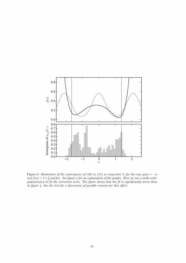
To test this conjecture we perform a numerical experiment, similar to the one for conjecture 3;the result is shown in figure 6. The fit between predicted and numerically determined correctionterm in figure 6 is worse than in figure 4 and thus the numerical test is not entirely conclusive.

One possible reason is that the spatial resolution of our numerical simulations may notbe sufficient. Indeed, the argument of the previous sections is based on a spatial averagingof the small-scale fluctuations of the process. In the case of multiplicative noise, these small-scale fluctuations are themselves multiplied by a the process f(u), which is spatially quite rough.Therefore, this spatial averaging will hold only on extremely small scales, where f(u) is essentiallyconstant. In order to be seen by the numerical simulation, these scales still need to be resolvedat sufficient precision to have some version of the law of large numbers.

4 Small Noise/Viscosity Limit

One regime that is of particular interest is the small noise/small viscosity limit. If one takesν ∝ σ2 in conjectures 1 and 2, one obtains a non-vanishing correction term even for arbitrarilysmall ν and σ! It is therefore of interest to study approximations to

du = ε ∂2xu dt− u ∂xu dt+√ε dw (32)

for ε� 1.It is well-known that, in the limiting case ε = 0, finite difference schemes for the Burgers

equations can only be used with extreme caution due to the presence of shocks in the solution.These shocks are jump discontinuities of the solution. The values u−, u+ to the left/right ofthe jumps satisfy u− > u+; in other words, the jumps are always downwards jumps. Forviscosity solutions2 to the inviscid Burgers equation, shocks move through the system at velocity12 (u+ + u−).

What happens at the formation of a shock? If the limiting non-viscous Burgers equation isdiscretised as

∂tun = −unun+1 − un

δ, (33)

we expect the discretisation scheme to be stable only when the discretisation is upwind in thesense that the direction of the discretisation coincides with the direction of propagation of the

2Also called entropy solutions, these are the solutions that are obtained as limits of (32) as ε → 0

13

0.0

0.2

0.4

0.6

0.8

p(u

)

�2 �1 0 1 2u

0.00.10.20.30.40.50.60.70.8

hist

ogra

m o

f u1,0(T

,·)

Figure 6: Illustration of the convergence of (30) to (31) in conjecture 5, for the case g(u) = −uand f(u) = 1+ 1

2 cos(3u). See figure 4 for an explanation of the graphs. Here we use a sixth-orderpolynomial p to fit the correction term. The figure shows that the fit is significantly worse thanin figure 4. See the text for a discussion of possible reasons for this effect.

14

shock (see e.g. [CIR52, MRTB05]), but even in this case we expect the shock to propagate atthe wrong speed.

Another problem is the following one: In the case of a non-conservative discretisation ofthe type (33), a simple linear stability analysis reveals that the discretised solutions developan ultraviolet instability (i.e. the mode vn = (−1)n becomes unstable) in the regions whereu > 0. Similarly, the corresponding left-sided discretisation shows an instability in the regionswith u < 0. In contrast, for the case of a centred discretisation, the highly oscillatory modes arestable independently of the sign of u.

Remark 4.1 Conservative discretisations, i.e.

∂tun = − 1

2δ

(u2n+1 − u2n

),

or variants thereof, still require the scheme to be upwind for stability, but in this case the shocksof the discretised system propagate at the correct speed. Also, these schemes do not suffer fromthe ultraviolet instability.

How is this picture modified for non-zero values of ε? The instabilities discussed above growat a speed O(δ−1) while the stabilising effect of the viscosity is of the order εδ−2. Thus, oneexpects the viscosity to dominate only if ε� δ. Regarding the behaviour after the formation ofa shock, a simple boundary layer analysis shows that a typical shock for (32) has width O(ε),so that the caveats pointed out above are expected to become relevant as soon as ε . δ (see forexample [EVE00a] for a more sophisticated boundary layer analysis that even goes to the nextorder in ε).

On the other hand, at least away from shocks, the analysis performed in section 2 holds assoon as u can be approximated by the solution to the linearised equation at sufficiently small (butstill much larger than δ) spatial scales. The kth mode presents spatial features on a lenghtscaleof order k−1 and the nonlinearity essentially propagates the solution through space at speedsof order 1. Thus, the timescale on which the kth mode varies due to the nonlinear effects isexpected to be of order k−1. On the other hand, the relevant timescale of the linear part forthis mode is (εk2)−1 and we can conclude from this heuristic consideration that the linearisedequation is a good approximation to the full solution for modes with k � ε−1, i.e. on spacescales much smaller than ε. Consequently, one again expects the results from section 2 to berelevant as long as ε� δ. This leads to the following statements.

Conjecture 6 For ε � 1, we expect the solution to the finite difference approximation of (32)to show the following behaviour.

1. For δ � ε, the discretised solution converges to the viscosity solution of

∂tu = −1

2∂x(u2) +

c

4, (34)

where c ∈ {1, 0,−1} depending on whether the discretisation is right-sided, centred, orleft-sided. Neither of the instabilities discussed above occur.

2. For ε � δ, both viscosity and the noise term become irrelevant; the solution behaves likethe corresponding approximation to the inviscid Burgers equation. In particular, as long asthere are no shocks and while solutions have the correct sign to prevent ultraviolet blow-up,we expect to converge to (34) with c = 0. After the occurrence of a shock, one expectsstability only if the scheme is upwind and, for discretisations of type (33), shocks will havethe wrong propagation speed.

To test this conjecture we again perform a numerical experiment. Keeping in line with thetopic of this article, we focus on studying how the presence of the extra c/4 term in (34) is affectedby the values ε, δ > 0. For our experiment, we first solve the limiting equation (34) numericallyup to a time t > 0, once with c = 0 and once with c = 1, to get states u0(t), u1(t) ∈ L2

([0, 2π],R

).

Now, for given ε, δ > 0, we solve the right-sided finite difference discretisation (13) for (32) toget a solution uε,δ(t). According to conjecture 6 we expect uε,δ(t) ≈ u1 for δ � ε � 1 anduε,δ(t) ≈ u0 for ε� δ.

15

c = 1c = 0

ε=10−1

ε=10−2

ε=10−3

ε=10−4

ε=10−5

δ = 10−4.0δ = 10−3.5

δ = 10−3.0

ε=10−1

ε=10−2

ε=10−3

ε=10−4

ε=10−5

δ = 10−2.5

Figure 7: Illustration of the limiting behaviour of a right-sided finite difference discretisationfor (32) as ε ↓ 0 (for fixed δ). Distances are shown in “two-centre bipolar coordinates” asdescribed in the text. One can see that, as ε gets small, the finite difference discretisation firstgets close to the solution of (34) for c = 1 but then finally converges to the solution with c = 0 as εgets smaller than δ. This behaviour reflects the dichotomy between the two cases of conjecture 6.

To verify this conjecture, in figure 7 we consider, for fixed δ, the solution uε,δ(t) as a functionof ε. The coordinate system is chosen such that the (two dimensional) distance of uε,δ(t) tothe point c = 0 in the graph equals

∥∥uε,δ(t) − u0‖L2 ; similarly the distance of uε,δ(t) to the

point c = 1 in the graph equals∥∥uε,δ(t) − u1‖L2 (this is sometimes called “two-centre bipolar

coordinates”). The simulation indicates that the transition from c = 1 to c = 0 takes place ataround ε ≈ δ as expected.

A Simulations

To verify the heuristic arguments presented above, the text utilises a series of numerical results.This appendix summarises some of the technical aspects of these simulations.3

We first describe how to implement the finite difference schemes used to discretise SPDEslike (4), (21) and (29): For the space discretisation of these equations we approximate statesu ∈ L2

([0, 2π],R

)by vectors uN ∈ RN . The space discretisation of the differential operators

given by formula (12), above. The finite difference discretisation of the white noise process w isWN/

√∆x, where WN is a standard Brownian motion on RN and ∆x = δ = 2π/N is the space

grid size. This leads to RN -valued stochastic differential equations of the form

duN = νLNuN dt+ FN (uN ) dt+ σ(uN )

√1

∆xdWN (t)

where LN ∈ RN×N is the discretisation of the linear part and FN : RN → RN is the discretisationof the nonlinearity.

For discretising time we use the θ-method

u(n+1) = u(n) + νLN(θu(n+1) + (1− θ)u(n)

)∆t

+ FN(u(n)

)∆t+ σ(u(n))

√∆t

∆xξ(n),

where ∆t > 0 is the time step size, u(n) is the discretised solution at time n∆t, the ξ(n) are i.i.d.,N -dimensional standard normally distributed random variables, and θ = 1/2. Rearranging this

3For full details we refer to the source code of the programs used in these simulations, which is available fordownload at http://seehuhn.de/programs/HairerVoss10 .

16

equation gives (I − νθ∆tLN

)u(n+1) =

(I + ν(1− θ)∆tLN

)u(n)

+ FN (u(n)) ∆t+ σ(u(n))

√∆t

∆xξ(n).

(35)

Relation (35) allows to compute u(n+1) from u(n); since I − νθ∆tLN is cyclic tridiagonal, thissystem can be solved efficiently.

Since we are using the partially implicit θ-method for the linear part of the SDE, there areno constraints on the time step size ∆t arising from this term; on the other hand, since thenon-linear transport term is treated explicitly, one has to make sure that v∆t/∆x < C, wherev is the largest speed of propagation appearing in the solution and C is the Courant number,thus ensuring that the CFL condition is satisfied. The resulting method can be used to performthe simulations required to generate figures 1, 5 and 7, as well as the “finite difference” curve infigure 2.

As described in section 2, we can compute a spectral Galerkin approximation to the secondorder differential operator using discrete Fourier transform. This corresponds to replacing LNin (35) with

LN = F−1DF

where D = diag(−02,−12, . . . ,−bN/2c2

)and F : RN → CbN/2c+1 represents the discrete Fourier

transform (since the data is real, only bN/2c+1 of the Fourier coefficients need to be considered).Because the matrix LN is no longer tridiagonal, one should not try to explicitly construct thismatrix. Instead one can use the fact that F and F−1 can be computed efficiently: we cancompute the right-hand side of (35) using(

I + ν(1− θ)∆tLN)u(n) = F−1 diag

(1− ν(1− θ)∆t k2, k = 0, . . . , bN/2c2

)F u(n)

and to solve (35) for u(n+1) we can use the relation(I − νθ∆tLN

)−1b = F−1 diag

( 1

1 + νθ∆t k2, k = 0, . . . , bN/2c2

)F b.

This technique allows to obtain the “Galerkin” curve in figure 2. Similarly, the rougher-than-white noise for figure 3 was obtained by replacing the noise term ξ(n) with

ξ(n) = F−1 diag((1 + k2)−δ, k = 0, . . . , bN/2c

)F ξ(n).

Finally, for the minimisation procedure performed to generate figures 4 and 6 we employ thesimplex algorithm by Nelder and Mead [NM65].

References

[AG06] A. Alabert and I. Gyongy. On numerical approximation of stochastic Burgers’ equa-tion. In From stochastic calculus to mathematical finance, pp. 1–15. Springer, Berlin,2006.

[Bar96] A.-L. Barabasi. Roughening of growing surfaces: Kinetic models and continuumtheories. Computational Materials Science, vol. 6, no. 2, pp. 127–134, 1996. doi:10.1016/0927-0256(96)00026-2. Proceedings of the Workshop on Virtual MolecularBeam Epitaxy.

[BCF91] Z. Brzezniak, M. Capinski and F. Flandoli. Stochastic partial differential equationsand turbulence. Math. Models Methods Appl. Sci., vol. 1, no. 1, pp. 41–59, 1991.doi:10.1142/S0218202591000046.

[BCJL94] L. Bertini, N. Cancrini and G. Jona-Lasinio. The stochastic Burgers equation. Comm.Math. Phys., vol. 165, no. 2, pp. 211–232, 1994.

17

[BFG+94] G. Blatter, M. V. Feigel’man, V. B. Geshkenbein, A. I. Larkin and V. M. Vinokur.Vortices in high-temperature superconductors. Rev. Mod. Phys., vol. 66, no. 4, pp.1125–1388, 1994. doi:10.1103/RevModPhys.66.1125.

[BG97] L. Bertini and G. Giacomin. Stochastic Burgers and KPZ equations from particlesystems. Comm. Math. Phys., vol. 183, no. 3, pp. 571–607, 1997. doi:10.1007/s002200050044.

[BM96] J.-P. Bouchaud and M. Mezard. Velocity fluctuations in forced Burgers turbulence.Phys. Rev. E, vol. 54, no. 5, pp. 5116–5121, 1996. doi:10.1103/PhysRevE.54.5116.

[BQS09] M. Balazs, J. Quastel and T. Seppalainen. Scaling exponent for the Hopf-Cole solu-tion of KPZ/Stochastic Burgers, 2009. Preprint.http://arxiv.org/abs/0909.4816

[CIR52] R. Courant, E. Isaacson and M. Rees. On the solution of nonlinear hyperbolic differ-ential equations by finite differences. Comm. Pure. Appl. Math., vol. 5, pp. 243–255,1952.

[DPDT94] G. Da Prato, A. Debussche and R. Temam. Stochastic Burgers’ equation. NoDEANonlinear Differential Equations Appl., vol. 1, no. 4, pp. 389–402, 1994. doi:10.1007/BF01194987.

[DPZ92] G. Da Prato and J. Zabczyk. Stochastic Equations in Infinite Dimensions, vol. 44of Encyclopedia of Mathematics and its Applications. Cambridge University Press,1992. ISBN 0-521-38529-6.

[EKMS00] W. E, K. Khanin, A. Mazel and Y. Sinai. Invariant measures for Burgers equationwith stochastic forcing. Ann. of Math. (2), vol. 151, no. 3, pp. 877–960, 2000.

[EVE00a] W. E and E. Vanden Eijnden. Another note on forced Burgers turbulence. Phys.Fluids, vol. 12, no. 1, pp. 149–154, 2000.

[EVE00b] W. E and E. Vanden Eijnden. Statistical theory for the stochastic Burgers equationin the inviscid limit. Comm. Pure Appl. Math., vol. 53, no. 7, pp. 852–901, 2000.

[GD04] C. Gugg and J. Duan. A Markov jump process approximation of the stochasticBurgers equation. Stoch. Dyn., vol. 4, no. 2, pp. 245–264, 2004.

[GKN02] C. Gugg, H. Kielhofer and M. Niggemann. On the Approximation of the StochasticBurgers Equation. Communications in Mathematical Physics, vol. 230, no. 1, pp.181–199, 2002.

[GM05] B. Goldys and B. Maslowski. Exponential ergodicity for stochastic Burgers and 2DNavier-Stokes equations. J. Funct. Anal., vol. 226, no. 1, pp. 230–255, 2005.

[GN99] I. Gyongy and D. Nualart. On the stochastic Burgers’ equation in the real line. Ann.Probab., vol. 27, no. 2, pp. 782–802, 1999.

[GSS85] S. N. Gurbatov, A. I. Saichev and S. F. Shandarin. A model description of thedevelopment of the large-scale structure of the Universe. Dokl. Akad. Nauk SSSR,vol. 285, no. 2, pp. 323–326, 1985.

[Gyo98] I. Gyongy. Existence and uniqueness results for semilinear stochastic partial differ-ential equations. Stochastic Process. Appl., vol. 73, no. 2, pp. 271–299, 1998.

[Hai09] M. Hairer. An Introduction to Stochastic PDEs. Lecture notes, 2009.http://arxiv.org/abs/0907.4178

[HSV07] M. Hairer, A. M. Stuart and J. Voss. Analysis of SPDEs Arising in Path Sampling,Part II: The Nonlinear Case. Annals of Applied Probability, vol. 17, no. 5, pp.1657–1706, 2007. doi:10.1214/07-AAP441.

18

[Kim06] J. U. Kim. On the stochastic Burgers equation with a polynomial nonlinearity in thereal line. Discrete Contin. Dyn. Syst. Ser. B, vol. 6, no. 4, pp. 835–866 (electronic),2006.

[Kra99] R. H. Kraichnan. Note on forced Burgers turbulence. Phys. Fluids, vol. 11, no. 12,pp. 3738–3742, 1999.

[MRTB05] R. M. M. Mattheij, S. W. Rienstra and J. H. M. ten Thije Boonkkamp. Partial Differ-ential Equations. SIAM Monographs on Mathematical Modeling and Computation.Society for Industrial and Applied Mathematics (SIAM), 2005. ISBN 0-89871-594-6.

[NM65] J. Nelder and R. Mead. A Simplex Method for Function Minimization. ComputerJournal, vol. 7, pp. 308–313, 1965.

[SZ89] S. F. Shandarin and Y. B. Zel’dovich. The large-scale structure of the universe: tur-bulence, intermittency, structures in a self-gravitating medium. Rev. Modern Phys.,vol. 61, no. 2, pp. 185–220, 1989.

[TZ06] K. Twardowska and J. Zabczyk. Qualitative properties of solutions to stochas-tic Burgers’ system of equations. In Stochastic partial differential equations andapplications—VII, vol. 245 of Lect. Notes Pure Appl. Math., pp. 311–322. Chapman& Hall/CRC, Boca Raton, FL, 2006.

[YC96] V. Yakhot and A. Chekhlov. Algebraic Tails of Probability Density Functions in theRandom-Force-Driven Burgers Turbulence. Phys. Rev. Lett., vol. 77, no. 15, pp.3118–3121, 1996. doi:10.1103/PhysRevLett.77.3118.

19