SIAM J. NUMER. ANAL.Vol. 4, No. 1, 1967Printed in U.S.A.

APPROXIMATIONS AND BOUNDS FOR EIGENVALUES OFELLIPTIC OPERATORS*

L. FOX, P. HENRICI$ AND C. MOLER1. Introduction. Let G be a bounded, n-dimensional domain with bound-

ary F. Let p(x) and q(x), i 1, n, be positive functions defined onand let D denote the linear, self-adjoint differential operator defined by

Du 0 Ou:

q

The eigenvalue problem for D on G involves the nonzero solutions k andu(z) of

(1.1) Du(x) q- kp(x)u(x) 0, x E G,

with the boundary condition

(1.2) u(x) o,The eigenfunctions may be normalized so that

(1.3)

where

(.4)

1M fa u(x)p(x) dx 1,

M fa p(x) dx.

xEP.

* Invited paper presented May 13, 1966, at the Symposium on Numerical Solution ofDifferential Equations, SIAM 1966 National Meeting at the University of Iowa,sponsored by the Air Force Office of Scientific Research.

f Oxford University Computing Laboratory.: Eidgenhssische Technische Hochschule, Zurich, and IBM Zurich Research Lab-

oratory, 8803 Rfischlikon-ZH, Switzerland.Eidgenhssische Technische Hochschule, Zurich. Present address: University of

Michigan, Ann Arbor, Michigan.

89

We are interested in computing accurate approximations to the eigen-values and their corresponding eigenfunctions. Furthermore, we want toestimate the accuracy of our approximations by using them to computeupper and lower bounds for the true eigenvalues.

In 2 we prove the following theorem which is the basis for these upperand lower bound calculations.THEOREM. Let X* and u* be an approximate eigenvalue and eigenfunction

which satisfy (1.1) and (1.3), but not necessarily (1.2). Let

(.5) max

Dow

nloa

ded

10/2

7/14

to 3

8.98

.219

.157

. Red

istr

ibut

ion

subj

ect t

o SI

AM

lice

nse

or c

opyr

ight

; see

http

://w

ww

.sia

m.o

rg/jo

urna

ls/o

jsa.

php

90 L. FOX ). HENRICI AND C. MOLER

and assume e < 1. Then there exists an eigenvalue ) ofD on G satisfying

k* 1 e"

The proof will use he fc h mxmum principle holds for heopera,or D; ha is, if s ny function for which

Ow(x) O, x G,(1.7)

then

(1.8) mx lw(x) _-< max w(x) !.xEq xEF

In 3 we outline a general technique for constructing a X* and u* whichcan produce an arbitrarily small in (1.5).In 4 we specialize to two-dimensional domains and take D to be the

Laplacian A. We describe the method of collocation by interpolationfor finding ),* and u*. This method is particularly suitable for domains withsymmetry and domains with corners, that is, where a portion of F consists oftwo intersecting straight line segments.

In 5 we illustrate the method by applying it to elliptical domains ofvarying eccentricity.

In 6 we consider a much-studied example of a domain with corners,the L-shaped union of three unit squares. Its largest angle is -r and thus isreentrant. For this example our method has proved significantly moreaccurate than any other known method. In fact, the upper and lowerbounds obtained are even more precise than the approximations withoutbound obtained by other methods. For the first (smallest) eigenvalue ofthe L, for example, we show that

9.6397238 -<_ kl -<_ 9.6397239.

Finite difference methods have been used and analyzed for these problemsby Forsythe and Wasow [4], Fox [5], Moler [9], Veidinger [13] and others.However, convergence of these methods is quite slow for domains withreentrant corners. Difference methods in combination with collocationand conformal mapping have been used by Reid and Walsh [10] for theL, but their techniques become quite involved for more complicateddomains.The method of intermediate problems (A. Weinstein [14]) gives upper

and lower bounds for certain domains. For example, Stadter [11] uses themethod for rhombical domains.

Collocation methods similar to the one we describe in 4, but withoutthe upper and lower bounds, have also been developed by J. Reid and B.

Dow

nloa

ded

10/2

7/14

to 3

8.98

.219

.157

. Red

istr

ibut

ion

subj

ect t

o SI

AM

lice

nse

or c

opyr

ight

; see

http

://w

ww

.sia

m.o

rg/jo

urna

ls/o

jsa.

php

EIGENVALUES OF ELLIPTIC OPERATORS 91

Martin of the University of Sussex and J. WMsh of the University ofManchester.

2. Proof of the theorem. The proof of our theorem is based on thefollowing result which occurs in many forms in the literature. Collatz [2]attributes it to Kryloff and Bogoliubov and to D. H. Weinstein.LEMMA. Let A be a self-adjoint operator on a Hilbert space with inner

product .,. ). Let X, and u be the eigenvalues and orthonormal eigenfunctionsof A. Assume IX,I has no finite accumulation point. Let v be any element inthe space spanned by {u} and let

(v, Av) (the Rayleigh quotient)

and

<2o2> !1 A

Then ( >-_ p and there exists at least one eigenvalue kk satisfying

(2.3) p / p =< kk =< p -t- /’ p.For completeness we give the following proof. Let v _, a,,u,,. Then

Thus

I]<A pr)

E an

>- min (M 0)

(Xk p) for some

from which the conclusion (2.3) follows.In proving the theorem, we take the operator A to be -D and the inner

product to be

(2.4) (f, g) f(x)g(x)p(x) dx.

In the norm thus introduced the normalization becomes

The approximate eigenfunction u* is not quite acceptable as the test

Dow

nloa

ded

10/2

7/14

to 3

8.98

.219

.157

. Red

istr

ibut

ion

subj

ect t

o SI

AM

lice

nse

or c

opyr

ight

; see

http

://w

ww

.sia

m.o

rg/jo

urna

ls/o

jsa.

php

92 L. Fox P. HENRICI AND C. MOLER

function v of the lemma because it is not zero on all of the boundary andhence is not in the space spanned by /u}. Let w be the solution to theboundary value problem

Dw(P) O, P G,(2.5)

w(P) u*(P), P F,and let

(2.6) v u* w.

Then v satisfies the conditions of the lemma. We shall not need to actuallycalculate w, but shall only need to estimate its norm.

Defining

(2.7) 11 to IIand

(2.8) cos(u*, w)

we find, after a short manipulation, that

(2.9) p :i: /-i p ),* 1 cos -1- 2cosO+

Hence there exists N k with

(2.10) IX h*[ < max I cos 0 sinh* 1- 2cos0 +

where the maximum is over the two terms obtained with theFrom the identity

+ cos0+ sin0--1 - 1 2wcos0+

0 0 (( cos 0 sin 0)(1 2)(1 2 cos 0 + 2)

and the fact that if w2 < 1 the quantity on the right is nonnegative forall 0, we conclude

(2.11) ]cos0sin0-[ <+ for all1 2cos0+ 1-

By (2.4), (1.8) and (2.5) we have

(2.12) -<- max w --<- max u(

Dow

nloa

ded

10/2

7/14

to 3

8.98

.219

.157

. Red

istr

ibut

ion

subj

ect t

o SI

AM

lice

nse

or c

opyr

ight

; see

http

://w

ww

.sia

m.o

rg/jo

urna

ls/o

jsa.

php

EIGENYALUES OF ELLIPTIC OPERATORS 3

Finally, combining (2.10)-(2.12) we find

X* I e

which establishes the theorem.

3. The method of particular solutions. In order to make use of theTheorem, we must have a constructive method for obtaining * and u*.One available approach can be based on the method of particular solutionsdeveloped independently by S. Bergman [1] and I. N. Vekua [12] (see also[6] and [7]). We explain it briefly for two-dimensional domains in whichq(x, y) q(x, y). In this case (1.1) becomes

(3.1) Lu /u - (q/q)u - (q/q)u - )(p/q)u O.

It is also assumed that q/q, q/q and p/q are entire analytic functions andthat G is simply connected and contains the origin.By writing the elliptic operator as a formally hyperbolic operator in the

variables z x iy and z* x iy, and applying Riemnn’s method ofintegration, it is possible to set up in a natural way a linear one-to-onemapping u f[f, f*] of the pairs (f, f*) of functions of the single complexvariable z holomorphic in G and G*, respectively, and satisfyingf(O) f*(O), onto the complex-valued functions u satisfying (3.1). Theinverse mpping is defined by

z f*(z) uf(z) u

By taking f and f* to be powers of z, au infinite sequence of purticularsolutions is constructed"

u0(x, y) f[1, 1],(3.2)

u_(x,y) f[z, 0], u(x, y) 2[0, z], n 1, 2, .-..

Finite linear combinations of these solutions

(3.3) cu( x, y)j-----0

may be used for the approximate eigenfunction. The operator L andhence the linear combination (3.3) depend upon ),. Thus ) and the c arechosen to make the e in (1.5) as small as possible.The mapping is continuous in the Chebyshev norm in each compact

subdomain of G. It thus follows from standard approximation theoremsof one complex variable that any eigenfunction u regular in G can be ap-proximated, uniformly in any compact subdomain of G, by the linear corn-

Dow

nloa

ded

10/2

7/14

to 3

8.98

.219

.157

. Red

istr

ibut

ion

subj

ect t

o SI

AM

lice

nse

or c

opyr

ight

; see

http

://w

ww

.sia

m.o

rg/jo

urna

ls/o

jsa.

php

4 L. FOX P. HENRICI AND C. MOLER

binations (3.3). If G is a Jordan domain, and if u is sufficiently smooth onthe closure of G, then it follows from a theorem of Walsh [12] that u canbe approximated in the Chebyshev norm by linear combinations (3.3)even on the closure of G.

4. Collocation by interpolation. The remainder of the paper is concernedwith two-dimensional domains and

2 02

For this operator, the method of particular solutions produces

(4.1) u*(r, O)where (r, 0) are polar coordinates in G and J(. is the th order Besselfunction. The values of a, )* and c are to be determined.There are two classes of domains for which the at are determined in a

natural way. The first class includes domains which, when centered at theorigin, are symmetric with respect to both the x and y axes. If aj 2j,j 0, .-.,N 1, then

N--1

(4.2) u*(r,’=0

retains the known symmetries of the first eigenfunction. Similar choicesapply to other symmetries and higher eigenvalues.The second class of domains involve those for which F contains a corner

with angle - for some a _-> 1/2. The origin is taken as the vertex of the angle,

0 and - correspond to the two straight line segments forming the

angle and i jc, j 1, N. Then

(4.3) u*(r, ) cJ,(.V/-r sin ja0

automatically satisfies the boundary condition on the sides of the angleand has the correct asymptotic singularity at the corner.There are several possible methods for determining suitable values for

)* and c. Possibly the simplest is to pick N points, (r, ), ] 1, N,on the boundary F and interpolate the boundary condition at these points.Thus we require

(4.4) u*(r O) O, ]c 1, N.

Using the u* of (4.3) for illustration, if we let

(4.5)as ai()) J,(%/-r) sin cO,

A() be the N X N matrix a()) },

Dow

nloa

ded

10/2

7/14

to 3

8.98

.219

.157

. Red

istr

ibut

ion

subj

ect t

o SI

AM

lice

nse

or c

opyr

ight

; see

http

://w

ww

.sia

m.o

rg/jo

urna

ls/o

jsa.

php

EIGENVALUES OF ELLIPTIC OPERATORS

and

then (4.4) becomes

(4.6) A(X)c 0.

We therefore define X* to be a root of the equation

(4.7) det (A(X)) 0.

For any root the approximate eigenfunction u* is obtained by solving (4.6)for the coefficients cj.

The resulting X* and u* depend upon N and upon the choice of theinterpolating points (r,, 0h). In our experiments we have usually chosenthe points to be equally spaced along r. We have also found it helpful toimpose conditions on the derivatives of u* at certain points. These con-ditions are used to help force the contour u* 0 to be close to I’ andthereby reduce maxr u* I.The u* defined in this way does not necessarily satisfy the normaliza-

tion condition (1.3). A lower bound for u* is required. Let Go be the,

largest circle or circular sector centered at the origin and contained in G.Let

(4.8) radius of Go.Then, again using (4.3) for illustration,

1 fo (u*(x))Ilu*]l>__ dx

N__1 _, c c fo Jk(r)J(r)r dr sin 0 sinM k,j=l

(Now, M is simply the area of G.) Since a is an integer times a, the set of

functions sin aO, j 1, N, is orthogonal on 0 O . Hence

(4.9) u* ]] > 1 c Jo J(r)r dr.M 2 =

If u* is given by (4.2), then a should be taken as {.The Bessel function integrals occurring here can be expressed in terms

of values at r by using formulas proved, for example, in Courant-Hil-bert [3]"

1"’ =16,{ ( +(1 )J,(6)}(4.10) J,(,r)r dr 5 J" )

Dow

nloa

ded

10/2

7/14

to 3

8.98

.219

.157

. Red

istr

ibut

ion

subj

ect t

o SI

AM

lice

nse

or c

opyr

ight

; see

http

://w

ww

.sia

m.o

rg/jo

urna

ls/o

jsa.

php

96 L. FOX P. HENRICI AND 12, MOLER

(4.11) J (/t) J(#/t) J+l(gi).

The important quantity occurring in the upper and lower bounds is, ofcourse, e maXer[U*(X)I. For a given domain it may be possible toobtain a good estimate of this a priori (once the distribution of the Nboundary points is specified). However, we have chosen to calculate themaximum a posteriori. But this involves an additional theoretical problem:What is the error made in the computation of the error bounds? A com-plete rigorous analysis is, in principle, possible and would include a de-tailed study of the algorithm used to find max[u* as well as the roundofferrors in the other computations.

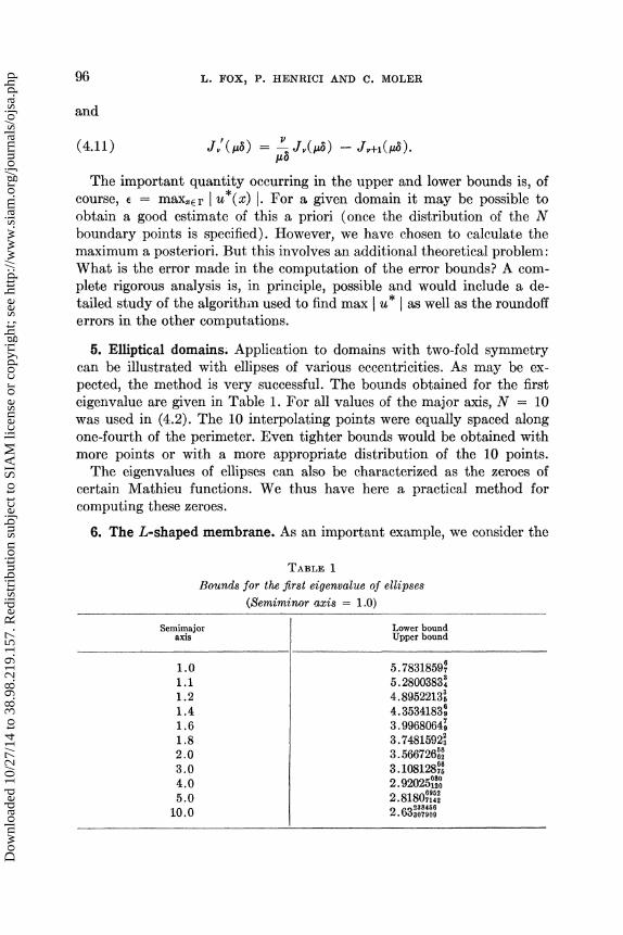
5. Elliptical domains. Application to domains with two-fold symmetrycan be illustrated with ellipses of various eccentricities. As may be ex-pected, the method is very successful. The bounds obtained for the firsteigenvalue are given in Table 1. For all values of the major axis, N 10was used in (4.2). The 10 interpolating points were equally spaced alongone-fourth of the perimeter. Even tighter bounds would be obtained withmore points or with a more appropriate distribution of the 10 points.The eigenvMues of ellipses can also be characterized as the zeroes of

certain Mathieu functions. We thus have here a practical method forcomputing these zeroes.

6. The L-shaped membrane. As an important example, we consider the

TABLE 1

Bounds for the first eigenvalue of ellipses

(Semiminor axis 1.0)

Semimajoraxis

1.0I.I1.21.41.61.82.03.04.05.010.0

Lower boundUpper bound

5.7831859.8ooa84.8952213

3.99680643.7481592

.o828o$o2.92025o

6952

2384562.

Dow

nloa

ded

10/2

7/14

to 3

8.98

.219

.157

. Red

istr

ibut

ion

subj

ect t

o SI

AM

lice

nse

or c

opyr

ight

; see

http

://w

ww

.sia

m.o

rg/jo

urna

ls/o

jsa.

php

EIGENVALUES OF ELLIPTI( OPERATORS 97

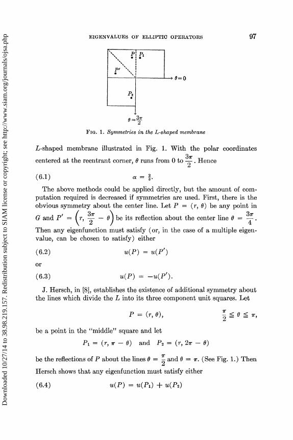
Fro. 1. Symmetries in the L-shaped membrane

L-shaped membrane illustrated in Fig. 1. With the polar coordinates

centered at the reentrant corner, t runs from 0 to . Hence

(6.1) a .The bove methods could be applied directly, but the amount of com-

putation required is decreased if symmetries are used. First, there is theobvious symmetry about the center line. Let P (r, 0) be any point in

GandP, ( 3r ) 3rr, -- 0 be its reflection about the center line 0 -.

Then any eigenfunction must satisfy (or, in the case of a multiple eigen-value, can be chosen to satisfy) either

(6.2) u(P) u(P’)or

(6.3) u(P) -u(P’).J. Hersch, in [8], establishes the existence of additional symmetry about

the lines which divide the L into its three component unit squares. Let

P (r, 0),

be a point in the "middle" square and let

P1 (r,r- 0) and P. (r, 2r- 0)

be the reflections of P about the lines t and 0 r. (See Fig. 1.) Then

Hersch shows that any eigenfunction must satisfy either

(6.4) u(P) u(P1) - u(P)

Dow

nloa

ded

10/2

7/14

to 3

8.98

.219

.157

. Red

istr

ibut

ion

subj

ect t

o SI

AM

lice

nse

or c

opyr

ight

; see

http

://w

ww

.sia

m.o

rg/jo

urna

ls/o

jsa.

php

98 L. FOX P. HENRICI AND (3. MOLER

or

(6.5) u is an eigenfunction of the unit square.

These symmetries have two consequences. First, we need only work in

the "first" square, 0 < O < r. Any approximation of u there can auto-

matically be extended to the other two squares. Second, requiring theapproximate eigenfunction u* to have the same symmetries as u sub-stantially reduces the number of terms necessary to obtain a given ac-curacy. For example, if u* is made to satisfy (6.2) and (6.4), then itfollows that

’=1

for all r and O. Hence, if ci 0,

1cos o 2 2

(6.7) a. a, 5a, 7a, lla, 13a, ....Thus, for a given N, replacing the original definition of a. (namely, as ja)with the above sequence increases the number of terms with nonzero c.by factor of three. Furthermore, u* is guaranteed to exhibit the propersymmetries.The sequence (6.7) follows from (6.2) and (6.4). These equutions hold,

for example, for the eigenfunction corresponding to the first eigenwlue.If, instead, we want u* to satisfy (6.3) and (6.4), we find

(6.8) a- 2a, 4a, 8a, 10a, 14a,

or, if u* stisfies (6.5),

(6.9) al 3a, 6a, 9a, ....The boundary points (rk, 0k) chosen on the perimeter of the first square

are spaced at an interval h, where 1/h is an integer. This defines 2/h points"

(rl,01) (%/i + h2,tan-lh),

(r, 0) (/ - 4h2, tn-1 2h),

(re/h, Oe/h) (1, r/2).

Dow

nloa

ded

10/2

7/14

to 3

8.98

.219

.157

. Red

istr

ibut

ion

subj

ect t

o SI

AM

lice

nse

or c

opyr

ight

; see

http

://w

ww

.sia

m.o

rg/jo

urna

ls/o

jsa.

php

EIGENVALUES OF ELLIPTIC OPERATORS 99

In addition we require

---0

at the two corners 1, 0) and (%/, r/4). Thus the total number of terms is

2N=-+ 2.

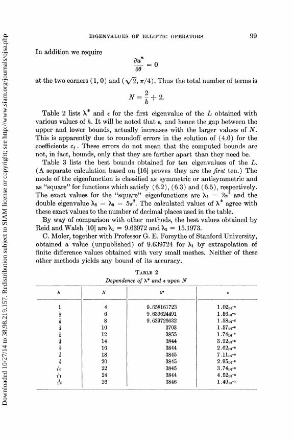
Table 2 lists )* and e for the first eigenvalue of the L obtained withvarious values of h. It will be noted that e, and hence the gap between theupper and lower bounds, actually increases with the larger values of N.This is apparently due to roundoff errors in the solution of (4.6) for thecoefficients c. These errors do not mean that the computed bounds arenot, in fact, bounds, only that they are farther apart than they need be.Table 3 lists the best bounds obtained for ten eigenvalues of the L.

(A separate calculation based on [16] proves they are the first ten.) Themode of the eigenfunction is classified as symmetric or antisymmetric andas "square" for functions which satisfy (6.2), (6.3) and (6.5), respectively.The exact values for the "square" eigenfunctions are )3 2r and thedouble eigenvalue s 9 5r. The calculated values of * agree withthese exact values to the number of decimal places used in the table.By way of comparison with other methods, the best values obtained by

Reid and Walsh [10] are 1 9.63972 and ) 15.1973.C. Moler, together with Professor G. E. Forsythe of Stanford University,

obtained a value (unpublished) of 9.639724 for )1 by extrapolation offinite difference values obtained with very small meshes. Neither of theseother methods yields any bound of its accuracy.

TAB,E 2

Dependence of X* and upon N

1 468101214161820222426

9.6581617239.6396244919.639726632

370338553844384438453845384538443846

1.02, 0-311.58,o-1.57,0-1.7410-’3.92, 0-82.62,0-97.11,0-92.95, 0-83.74,0-94.52,0-81.49,0-,

Dow

nloa

ded

10/2

7/14

to 3

8.98

.219

.157

. Red

istr

ibut

ion

subj

ect t

o SI

AM

lice

nse

or c

opyr

ight

; see

http

://w

ww

.sia

m.o

rg/jo

urna

ls/o

jsa.

php

100 L. FOX P. HENRICI AND (3. MOLER

TABLE 3Bounds for the first ten eigenvalues of the L

1234567

8, 910

Lower bound for knUpper bound for

9.639723S]1 2 18415. 97 5201

l.ne0i

31.912631141. 47451,59

flo46744.o5099.as06.7096

Mode of eigenfunction

symmetricantisymmetricsymmetric, squareantisymmetricsymmetricsymmetricantisymmetricmultiple, squaresymmetric

7. Other domains. In all fairness, it should be reported that results arenot always as satisfactory as these examples indicate. Experiments withrhombical domains were also made. These domains have both symmetryand a corner. However, we have been unable to obtain bounds signifi-cantly tighter than those obtained in [11] by other methods. The difficultystems from the existence of two corners with nonintegral values of a.

These singularities are reflected in the slow convergence of either (4.2)or (4.3) and consequent influence of roundoff errors in the coefficients.Other methods for defining and computing these coefficients are currentlybeing investigated.

8. Computational details. We conclude with a few remarks on thetechniques used in the computations.The Bessel functions are evaluated by truncating the alternating series

(8.1) g(x) x _, t,n-0

where t t_/(u(n + ) ). The value of to should be

1(s.2) to t0(,)2,r(, + 1)’

but it is not necessary to compute this gmm function since to is merely ascule fctor which can be absorbed into the coefficients c.. In fact, it isconvenient to use a value of to quite different from that given by (8.2)in order to scale J, to be about 1 for the arguments used. If this is done,it is not necessary to check for floating point exponent underflow and over-flow during the evaluation of the determinant (4.7).

(With a different value of t0(u), (4.12) should be replaced by

to(v) j+().)(4.11’) J,’(ti) - J,(ui)2( q- 1)-t0(u q- 1)

Dow

nloa

ded

10/2

7/14

to 3

8.98

.219

.157

. Red

istr

ibut

ion

subj

ect t

o SI

AM

lice

nse

or c

opyr

ight

; see

http

://w

ww

.sia

m.o

rg/jo

urna

ls/o

jsa.

php

EIGENVALUES OF ELLIPTIC OPERATORS 101

The function det (A (k)) is computed, using triangular decomposition(Gaussian elimination) with partial pivoting, for a few values of k near azero of the function. Then inverse interpolation is used several times tofind k*.

This use of inverse interpolation proves o be quie satisfactory for hesmaller eigenvlues of he L. Bu for he higher eigenvlues and for 11he eigenvlues of some oher domains sudied, he quniy de (A(k))hs local exremum very near k* nd i is herefore necessary o loceX* quie ceurely before inverse interpolation en be used.

Inverse ierion [15] is used o solve (4.6) for he coefficients. Inhe required ringulr decomposition of A(k*) hs lredy been computedduring he deerminn evaluation. Any reduction of he roundoff errorsincurred in he computed e his poin would led o igher upper ndlower bounds.

Finally, he clculion of mxlu*(P) on F is one-dimensionMmximizing problem. The boundary is broken into intervals by he points(rk, k). It is assumed that the only local minima of [u*[ occur, at thesepoints and thus a simple maximizing search is used on each interval. Ifanother local minimum is found, the search can be carried out on each ofthe resulting subintervals.Our computer program is written in ALGOL. A Control Data 1604A

with a 36-bit floating point significand was used. The calculation of onevalue of k* and the resulting bounds takes slightly over one minute forthe largest values of N shown. Most of this time is spent in the maximizingsearches on the boundary. Even so, this time represents a considerablereduction over the other methods which do not produce bounds.

Acknowledgments. Various parts of this paper were first presented intalks by the authors at the IBM Zurich Research Laboratory, Rfischlikon,Switzerland, and at the SIAM 1966 National Meeting, Iowa City.The computations were done at the Institute for Applied Mathematics ofthe Swiss Federal Institute of Technology. Moler’s work was supportedby the United States Office of Naval Research.

REFERENCES

[1] S. BERGMAN, Functions satisfying certain partial differential equations of elliptictype and their representation, Duke Math. J., 14 (1947), pp. 349-366..

[2] L. COLLATZ, Eigenwertprobleme und ihre Numerische Behandlung, AkademischeVerlagsgesellschaft, Leipzig, 1945, p. 208.

[3] R. COURANT AND D. HILBERT, Methods of Mathematical Physics, vol. 1, Inter-science, New York, 1953.

[4] G. :E. FORSYTHE AND W. n. WAsow, Finite-Difference Methods for Partial Differ-ential Equations, John Wiley, New York, 1962.

[5] L. Fox, Numerical Solution of Ordinary and Partial Differential Equations,Pergamon Press, Oxford, 1962.

Dow

nloa

ded

10/2

7/14

to 3

8.98

.219

.157

. Red

istr

ibut

ion

subj

ect t

o SI

AM

lice

nse

or c

opyr

ight

; see

http

://w

ww

.sia

m.o

rg/jo

urna

ls/o

jsa.

php

102 I. FOX P. HENRICI AND C. MOLER

[6] P. HENRICI, Zur Funktionentheorie der Wellengleichung, Comm. Math. Helv.,27 (1953), pp. 235-293.

[7] , A survey of I. N. Vekua’s theory of elliptic partial differential equationswith analytic coecients, Z. Angew. Math. Physik, 8 (1957), pp. 169-203.

[8] J. HERSCn, Erweiterte Symmetrieeigenschaften yon LOsungen gewisser linearerRand- und Eigenwertprobleme, J. Reine Angew. Math., 218 (1965), pp.143-158.

[9] C. MoLEn, Finite difference methods for the eigenvalues of Laplace’s operator,Report CS 22, Stanford University Computer Science Dept., 1965.

[10] J. K. REID hiD J. E. WALSH, An elliptic eigenvalue problem for a reentrant region,J. Soc. Indust. Appl. Math., 13 (1965), pp. 837-850.

[11] J. T. STADTEtt, Bounds to eigenvalues of rhombical membranes, Ibid., 14 (1966),pp. 324-341.

[12] I. N. VEKUA, Novya Metody Reenija Ellipticeskikh Uravnenij, (New Methodsfor Solving Elliptic Equations), O G I Z, Moscow and Leningrad, 1948.

[13] L. VEIDING.En, Compu.tation of the eigenvalues of a membrane by finite differencemethods, Zh. Vychisl. Mat. Mat. Fiz., 4 (1964), pp. 1037-1044.

[14] A. WEINSTEIN, Some numerical results in intermediate problems for eigenvalues,Numerical Solution of Partial Differential Equations, J. Bramble, ed.,Academic Press, New York, 1966.

[15] J. H. WILKINSON, The Algebraic Eigenvalue Problem, Oxford University Press,Oxford, 1965.

[16] J. HERSCH, Lower bounds for all eigenvalues by cell functions: a refined form ofH. F. Weinberger’s method, Arch. Rational Mech. Anal., 12 (1963), pp.361-366.

Dow

nloa

ded

10/2

7/14

to 3

8.98

.219

.157

. Red

istr

ibut

ion

subj

ect t

o SI

AM

lice

nse

or c

opyr

ight

; see

http

://w

ww

.sia

m.o

rg/jo

urna

ls/o

jsa.

php