Approximation and prediction of characteristic curves of ... · PDF fileECMI Modelling...

ECMI Modelling Workshop TU Eindhoven

Approximation and prediction of characteristic curves of

combustion engines

Group members:

Maria KudelaMatylda Jab lonskaVolha Shchetnikava

Leonie KarbachMagnus Dahler Norling

Daniel GerthViet Long NguyenChongrrui Zhou

Instructors:

Rene SchneiderHansjorg Schmidt

1

1 Description of the problem

We have a database containing characteristic data of about 1500 different combustion en-gines. As this data has been extracted from different sources, it varies in both the amount ofinformation present and in accuracy. Extracting information which may help in the designof new engines from such a large data set is of course challenging and the aid of automatedtools is required. The field of designing such automated tools is commonly described as”data mining”, and this project falls into this category.

Of special interest for the project is the curves describing the torque and the poweroutput in dependency on the rotation speed (RPM). For some of the engines in the data set,a spline is given which approximates a curve scanning form printed documents, for others,only the most basic data of the maximum of torque and power are given, and the RPMrange.

The fundamental aim of the project is to model the dependency of both curves on pa-rameters of the engine, that means the point of maximum torque and power, maximumdisplacement volume, stroke, number of cylinders, basic engine principle, etc. This is ap-proached by a number of intermediate steps:

a) Evaluation of the complete part of the data regarding consistency. After that, a con-sistent approximation of the given data is created.

b) Grouping of the data into distinct categories which share similar behaviour. Due tothe discrete nature of some of the parameters (e.g. number of cylinders) a continuousapproximation over the whole parameter range appears inappropriate. Currently thedata set is divided into categories according to engineers experience and intuition. Thisprocess is more or less automated. Two approaches are proposed, with different results.This sub-project is related to the field of pattern recognition.

c) Within each category, a model is generated which approximates the characteristiccurves in dependency on the engine parameters. For this purpose parametric modelsare defined suitably, and nonlinear least squares curve fitting techniques applied.

d) Based on c), an automated way should be found to extend the incomplete data sets inthe database to have an educated guess for the characteristic curves. Unfortunately,even though this part is quite simple compared with the others, we could not finish itas we ran out of time.

Note: All values of torque, power and RPM appear in this work have been scaled suchthat the copyright protected real data is not revealed. The units given are thus only forillustration and do not reflect values of actual engines. For an example of available powerand torque curves see Figure 1.

2

Figure 1: data curve

3

2 Consistency test and correction of the data

2.1 Description of working process and progress

In the given data of the engines torque and power values with corresponding rpm-values canbe found. Based on this information the aim is to test the consistency of the data and incase any problems occur, to correct them.

The data is considered consistent if it fulfills the equation T (ω) · ω = P (ω), that meansif the power is equal to the torque times the rpm-value, over the whole range of rpm-values.

The first problem hereby encountered is the different rpm-values that are given for torqueand power. Therefore it is not possible to easily compare the torque and power values, sinceevery rpm-value is only known for one of the torque and power values. While searching fora way to find the missing values, it became apparent that the given values define a spline asa parameterized curve, rather than a function.

The DeBoor algorithm interpolates the given data with DeBoor-Splines and evaluatesthe curve afterwards at any given point.

More in detail, the input is a point in the parameter interval and the given data and theoutput is then the ω and the corresponding torque or power value. After implementing thisalgorithm, one has now access to rpm-values and corresponding power and torque values.But the algorithm needs the described input and therefore another algorithm has to bewritten that would produce the corresponding input-point for a given ω.

To get the ω, the output of the DeBoor algorithm is restricted to just the first value,namely the ω. Then the Matlab-command fzero is used to get access to the point of interestby finding a zero of the restricted DeBoor minus ω, which is a kind of inversion of the actualDeBoor process. An example result is presented in Figures 2 and 3.

Figure 2: Given Data and Curve after DeBoor algorithm.(example)

4

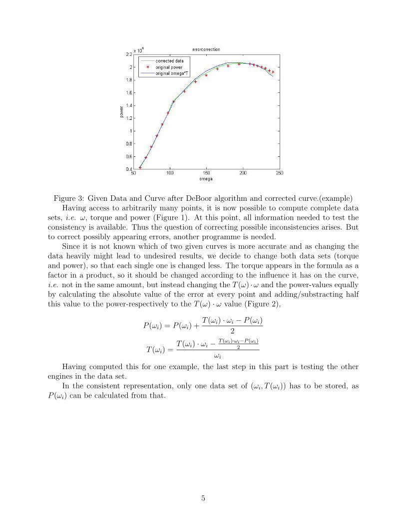
Figure 3: Given Data and Curve after DeBoor algorithm and corrected curve.(example)Having access to arbitrarily many points, it is now possible to compute complete data

sets, i.e. ω, torque and power (Figure 1). At this point, all information needed to test theconsistency is available. Thus the question of correcting possible inconsistencies arises. Butto correct possibly appearing errors, another programme is needed.

Since it is not known which of two given curves is more accurate and as changing thedata heavily might lead to undesired results, we decide to change both data sets (torqueand power), so that each single one is changed less. The torque appears in the formula as afactor in a product, so it should be changed according to the influence it has on the curve,i.e. not in the same amount, but instead changing the T (ω) ·ω and the power-values equallyby calculating the absolute value of the error at every point and adding/substracting halfthis value to the power-respectively to the T (ω) · ω value (Figure 2),

P (ωi) = P (ωi) +T (ωi) · ωi − P (ωi)

2

T (ωi) =T (ωi) · ωi − T (ωi)·ωi−P (ωi)

2

ωi

Having computed this for one example, the last step in this part is testing the otherengines in the data set.

In the consistent representation, only one data set of (ωi, T (ωi)) has to be stored, asP (ωi) can be calculated from that.

5

3 Curve grouping

3.1 Motivation

Since the full set of engines in the database have torque curves that are very different innature, it appears to be necessary to separate them into different groups. It would be verydifficult to make a model based on all the curves at once. We explored several ways of definingand determining whether two curves look similar. Then we tried to find an algorithm todetermine whether or not two engines have similar curves, based only on the attributes ofthese two engines. This is necessary, since no curve would be known for a new engine, indeedthe goal of the project was to find a way of estimating the torque and power curves of newengines based only on their attributes and known values of maximum torque and power, andthe rpm at which these are attained.

There are two aims of this section. The first is to present results of a manual searchfor patterns in the curves from the distance and attributes point of view. The second isto discuss an automated way of choosing a group of similar curves that would be used toapproximate the shape of curves for a new engine with given attributes.

3.2 Measuring the closeness of curves

The first idea for evaluation of the curves’ comparability is to create a metric on the spaceof curves that in some way tells how similar they are. This notion of closeness should reflecthow easy it would be to make common model for these curves.

We decided first to scale the curves, since many of the curves with similar shapes wouldbe different in size. We thought that the difference in overall shape was more critical indistinguishing the curves than their magnitudes and lengths. First we tried to scale them inthe value space by their own maximal value, so that each scaled curve would have maximalvalue one. Later we also scaled them in their domain so that the maxima of all curves wouldoccur in position (1, 1).

After the scaling, we let the distance between two curves c1 and c2 be determined bytheir L2 distance on their common domain of definition, i.e

d(c1, c2) =

∫D(c1)∩D(c2)

(c1(ω)− c2(ω))2dω

12

. (1)

As can be seen in Figure 4, the metric (1) groups together curves that have similarshape.

6

0 0.5 1 1.50

0.1

0.2

0.3

0.4

0.5

0.6

0.7

0.8

0.9

1Plot of a curve, surrounded by the curves closest to it after scaling

rpm (scaled)

Tor

que

(sca

led)

Figure 4: Curves that are close to a reference curve after scaling.

Figure 5 presents the whole set of scaled torque curves and and indicates how close eachcurve is to a reference curve that was randomly chosen beforehand.

0 1 2 3 4 5 6 70

0.1

0.2

0.3

0.4

0.5

0.6

0.7

0.8

0.9

1Plot of all the curves after scaling, with color given by distance to a specific curve (black is near)

rpm (scaled)

Tor

que

(sca

led)

Figure 5: The torque curves of all the engines, with closeness to a reference curve given bythe intensity of the color. Here black means close, and white means distant. The referencecurve is plotted in blue.

7

3.3 Discussion on the way to determine closeness of curves

The above mentioned metric (1) groups curves that have similar shapes together, but it maynot necessarily give groups that are easily distinguished by the attributes of the engines.Other methods of scaling should be tried. Scaling the curves in the value, may for instancenot be a good idea if several attributes determine the size of the curves in this direction,such as number of cylinders and displacement volume. Scaling then diminishes the impact ofthese attributes on the groupings, and makes it harder to find good groups based on these.On the other hand, we don’t want a model where the shape of the curve is determined byit’s maximal value, unless this is a trend present in the data.

A similar discussion is of course valid for the scaling in the domain direction. Theimportance of different attributes for the placement of the maximum of the curve should bethe topic of further research.

Other scaling methods may be used as well, such as dividing the power and torquecurve values by the number of cylinders, to look at the power per cylinder and torque percylinder curves. There has also been one idea to choose the scaled curves for approximationby location of their torque value at the point of maximal power. However, there has beennot enough time to verify this method.

3.4 Grouping by crucial attributes

The goal is then to determine whether two engines will have similar curves in the sense ofthe metrics discussed above, using information about the attributes of the engines.

For determining the importance of a few densely represented1 continuously distributedattributes, we looked at some random engines, and the engines that had curves closest tothem, and then we looked at how the attributes behaved within these groups. If we foundthat the mean value of a certain attribute within a group differed significantly from themean value over the entire set of engines, and if in addition the standard deviation of thatattribute within the group was low, that attribute was identified as a good indicator for thegrouping.

[htp]

Statistics for the 58 curves within distance 0.025 of curve 150,

followed by the statistics for the entire set:

ATTRIB_45: mean 4.74, stdev 1.07, ALL: mean 5.08, stdev 1.74





ATTRIB_324b: mean 65.62, stdev 7.57, ALL: mean 62.82, stdev 15.56

ATTRIB_323b: mean 350.75, stdev 20.29, ALL: mean 324.70, stdev 52.72



ATTRIB_48: A:58 B:0 ALL: A:1261 B:330

ATTRIB_55: A:0 B:58 ALL: A:543 B:1048

ATTRIB_282: A:32 B:2 E:0 F:0 C:0 D:0 ALL: A:723 B:394 E:7 F:2 C:3 D:6

ATTRIB_1132: A:11 B:2 ALL: A:204 B:69

1For some attributes, we only had data for very few engines, so we did not have enough information togo by to use them for anything useful.

8

Figure 6: Statistics for a group of engines created by our subroutine (slightly formatted forclarity). Attribute 48 signifies supercharged / non-supercharged, while attribute 55 signifiesotto / diesel. The last four lines, A, B, C, D, E, F are string-valued attributes. Calculatingmean value or standard deviation does not apply in this case, therefore we only give countof occurrences within the close curves’ group and the whole data set.

From Figure 6, we can see that the groupings made by the L2 metric (1) are not alwaysconsistent with grouping of attributes. For example, for attribute 58 both mean and standarddeviation of the close curves are very close to the whole sample results, whereas attribute 101shows considerably big difference between both average and variance. On the other hand, e.g.for attribute 323 the close curves have mean value very similar to the whole sample’s mean,whereas there is a huge contrast between the standard deviation magnitudes. Therefore,perhaps it is advisable to verify, whether partitioning by attributes reveals any clustering inthe curves’ shapes.

The features that may most intuitively influence the engine’s performance are:

• number of cylinders

• Otto/Diesel

• supercharged/non-supercharged

• displacement volume

This first observation comes from visual representation of different values for given at-tributes. To illustrate this, Figures 7 and 8 present original power and torque curves split indifferent colors by number of cylinders.

0 100 200 300 400 500 600 7000

0.2

0.4

0.6

0.8

1

1.2

1.4

1.6

1.8

2x 10

5

rpm

pow

er [W

]

Engine power curves split with respect to number of cylinders

Figure 7: Original power curves split in different colors by number of cylinders in a givenengine.

9

0 100 200 300 400 500 600 7000

100

200

300

400

500

600

700

rpm

torq

ue [N

m]

Engine torque curves split with respect to number of cylinders

Figure 8: Original torque curves split in different colors by number of cylinders in a givenengine.

We can see that the number of cylinders in an engine has a big influence on the spreadof power and torque values. There is clear clustering visible for both groups of curves.Therefore, if the idea of scaling data with respect to maximum values of the curves does notgive satisfactory results, scaling by number of cylinders may also be a way to adjust curvesto be more comparable by distance.

Next, we test separation of curves by the Otto/Diesel attribute. Figures 9 and 10.present results. We can see that Otto engines reach their maximum at lower value of RPMthan the Diesel ones.

0 50 100 150 200 250 300 350 400 450 5000

0.2

0.4

0.6

0.8

1

1.2

1.4

1.6

1.8

2x 10

4

rpm

pow

er [W

]

Engine power curves split by Otto/Diesel type

Figure 9: Original power curves split in different colors by Otto(blue)/Diesel(red) type of agiven engine.

10

0 50 100 150 200 250 300 350 400 450 5000

10

20

30

40

50

60

70

80

rpm

torq

ue [N

m]

Engine torque curves split by Otto/Diesel type

Figure 10: Original torque curves split in different colors by Otto(blue)/Diesel(red) type ofa given engine.

One more attribute influencing the engine performance may be the fact whether theengine is supercharged or not. Therefore, we analyse the power and torque curves from thatpoint of view. Results can be seen in Figure 11.

0 100 200 300 400 500 600 7000

0.5

1

1.5

2x 10

4

rpm

pow

er [W

]

Otto power curves − supercharged/non−supercharged

0 100 200 300 400 500 600 7000

10

20

30

40

50

60

70

80

rpm

torq

ue [N

m]

Otto torque curves − supercharged/non−supercharged

0 50 100 150 200 250 300 3500

5000

10000

15000

rpm

pow

er [W

]

Diesel power curves − supercharged/non−supercharged

0 50 100 150 200 250 300 3500

10

20

30

40

50

60

70

80

rpm

torq

ue [N

m]

Diesel torque curves − supercharged/non−supercharged

Figure 11: Original power (upper panels) and torque (bottom panels) curves split in differentcolors by supercharged(blue)/non-supercharged(pink) type of a given engine.

For Diesel engines there is only one non-supercharged model, thus it is difficult to makeany assessment. However, for Otto engines it is clear that the supercharged ones (blue) reach

11

higher values of power and torque than the non-supercharged ones.Now, when we succeeded to make a very general partitioning by some discrete attributes,

we can analyse also a continuously-valued one. Let us consider the engine’s displacementvolume. To be able to see visual differences between power and torque curves we split givendisplacement volume into intervals with step 0.4. Since the data was changed by the providerto be anonymous, the value 0.4 has only intuitive character; it is chosen to obtain a sufficientbut not too big number of groups. Figures 12 and 13 show this partitioning of curves forpower and torque respectively.

0 100 200 300 400 5000

0.5

1

1.5

2x 10

4

rpm

pow

er [W

]

power curves for otto/sup by disp. vol.

0 100 200 300 400 500 600 7000

2000

4000

6000

8000

10000

12000

14000

rpmpo

wer

[W]

power curves for otto/non−sup by disp. vol.

0 50 100 150 200 250 3000

2000

4000

6000

8000

10000

12000

rpm

pow

er [W

]

power curves for diesel/sup by disp. vol.

0 50 100 150 200 250 300 3500

1000

2000

3000

4000

5000

rpm

pow

er [W

]

power curves for diesel/non−sup by disp. vol.

Figure 12: Original power curves for different engines split in different colors by displacementvolume intervals.

12

0 100 200 300 400 5000

10

20

30

40

50

60

70

80

rpm

torq

ue [N

m]

torque curves for otto/sup by disp. vol.

0 100 200 300 400 500 600 7000

10

20

30

40

50

rpm

torq

ue [N

m]

torque curves for otto/non−sup by disp. vol.

0 50 100 150 200 250 3000

10

20

30

40

50

60

70

80

rpm

torq

ue [N

m]

torque curves for diesel/sup by disp. vol.

0 50 100 150 200 250 300 35018

19

20

21

22

23

24

25

rpmto

rque

[Nm

]

torque curves for diesel/non−sup by disp. vol.

Figure 13: Original torque curves for different engines split in different colors by displacementvolume intervals.

There is no obvious clustering visible in the supercharged group (upper/bottom leftpanel), but there appears to be significant clustering in the Otto non-supercharged fam-ily. The colors identifying different displacement volume intervals reveal clear layers withinthe whole data set. Therefore, we could also assume that displacement volume plays animportant role in the engine’s performance.

At this point we are interested in combining the previous idea of scaling with currentresults in grouping by attributes. As it was mentioned before, one of the steps in analysis wasto scale all the power and torque curves in the way that they all would have their maxima inpoint (1, 1). Now, using this set of curves, we test again the already performed separation.Figure 14 presents the scaled power curves for engines grouped by displacement volumeinterval: Otto/supercharged (upper left panel), Otto/non-supercharged (upper right panel),Diesel/supercharged (bottom left panel), Diesel/non-supercharged (bottom right panel).

13

0 0.5 1 1.5 20

0.2

0.4

0.6

0.8

1

rpm

pow

er [W

]

power curves for otto/sup by disp. vol.

0 0.5 1 1.5 20

0.2

0.4

0.6

0.8

1

rpm

pow

er [W

]

power curves for otto/non−sup by disp. vol.

0 0.5 1 1.50

0.2

0.4

0.6

0.8

1

rpm

pow

er [W

]

power curves for diesel/sup by disp. vol.

0 0.5 1 1.5 20

0.2

0.4

0.6

0.8

1

rpmpo

wer

[W]

power curves for diesel/non−sup by disp. vol.

Figure 14: Scaled power curves for different engines split in different colors by displacementvolume intervals.

We can see that especially for the Otto/non-supercharged family the engines with thesame interval of displacement volume are slightly concentrated. The Otto/supercharged setgives similar impression. In Figure 15 similar plots for scaled torque curves can be seen. Alsothe conclusion is similar: especially Otto engines’ curves reveal some concentration withinthe same displacement volume intervals.

14

0 1 2 3 4 5

0.4

0.5

0.6

0.7

0.8

0.9

1

rpm

torq

ue [N

m]

torque curves for otto/sup by disp. vol.

0 1 2 3 4 5 6 70

0.2

0.4

0.6

0.8

1

rpm

torq

ue [N

m]

torque curves for otto/non−sup by disp. vol.

0 0.5 1 1.5 2 2.5 3 3.50

0.2

0.4

0.6

0.8

1

rpm

torq

ue [N

m]

torque curves for diesel/sup by disp. vol.

0 0.5 1 1.5 2 2.5 30.75

0.8

0.85

0.9

0.95

1

rpmto

rque

[Nm

]

torque curves for diesel/non−sup by disp. vol.

Figure 15: Scaled torque curves for different engines split in different colors by displacementvolume intervals.

In this subsection we succeeded to identify the most general attributes that allow sig-nificantly clear partitioning on the power and torque curves. Nevertheless, the groups stillremain very general and should be narrowed down if possible.

3.5 Algorithm for grouping by discrete and continuous attributes

The aim of this subsection is to propose an algorithm for grouping curves by both discreteand continuous attributes. We try the method described in algorithm 1, which calculates anattribute-based distance d = d(e1, e2) between two given engines e1, e2. If d ≤ 1, the enginesare guessed to be close. w(a) are predetermined weigths for each attribute, based on howimportant we think it is in determining the closeness of the engines. The set E is the entireset of engines, and the set A is the set of attributes we think are useful enough to consider.

Algorithm 1 Proposed algorithm for guessing if two engines have similar curves.Input: e1,e2

if e1(type) 6= e2(type) or e1(charging) 6= e2(charging) thend := 2

elsed :=

∑a∈A

|e1(a)−e2(a)|·w(a)maxe∈E e(a)

end ifOutput: d

15

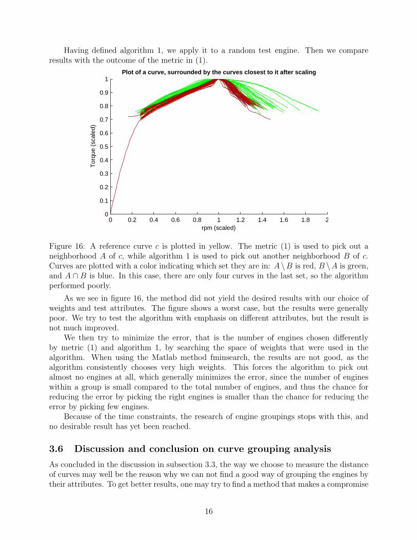
Having defined algorithm 1, we apply it to a random test engine. Then we compareresults with the outcome of the metric in (1).

0 0.2 0.4 0.6 0.8 1 1.2 1.4 1.6 1.8 20

0.1

0.2

0.3

0.4

0.5

0.6

0.7

0.8

0.9

1Plot of a curve, surrounded by the curves closest to it after scaling

rpm (scaled)

Tor

que

(sca

led)

Figure 16: A reference curve c is plotted in yellow. The metric (1) is used to pick out aneighborhood A of c, while algorithm 1 is used to pick out another neighborhood B of c.Curves are plotted with a color indicating which set they are in: A\B is red, B \A is green,and A ∩ B is blue. In this case, there are only four curves in the last set, so the algorithmperformed poorly.

As we see in figure 16, the method did not yield the desired results with our choice ofweights and test attributes. The figure shows a worst case, but the results were generallypoor. We try to test the algorithm with emphasis on different attributes, but the result isnot much improved.

We then try to minimize the error, that is the number of engines chosen differentlyby metric (1) and algorithm 1, by searching the space of weights that were used in thealgorithm. When using the Matlab method fminsearch, the results are not good, as thealgorithm consistently chooses very high weights. This forces the algorithm to pick outalmost no engines at all, which generally minimizes the error, since the number of engineswithin a group is small compared to the total number of engines, and thus the chance forreducing the error by picking the right engines is smaller than the chance for reducing theerror by picking few engines.

Because of the time constraints, the research of engine groupings stops with this, andno desirable result has yet been reached.

3.6 Discussion and conclusion on curve grouping analysis

As concluded in the discussion in subsection 3.3, the way we choose to measure the distanceof curves may well be the reason why we can not find a good way of grouping the engines bytheir attributes. To get better results, one may try to find a method that makes a compromise

16

between making it easy to group the engines by attributes and making it easy to fit a modelto the groups generated by this method. However, this may not be straightforward.

We recommend that a more thorough statistical analysis is conducted of the groupingand correlation between attributes within the groups. A new algorithm to replace algorithm1 should then be created based on the result from the analysis. If a method based on weightsis chosen, one needs to find a good way to optimize these weights, but this may not be easyto automatize since the problem may be very irregular. Fortunately, this optimization willonly have to be done once. Once good weights are found, the algorithm is ready to use.

17

4 Modeling the problem

4.1 Motivation

We want to create a model, which will approximate torque and power curves in dependencywith engine parameters. Some engines in the data set have approximately 20 values of torqueand power, which can be easily interpolated by a cubic spline. For the remaining enginesonly basic data is known.

The idea of our modeling is to approximate the characteristic curve with the help ofa cubic spline going through points. These are dependent on the engine parameters. Thenumbers of points are variable. We have used seven points as this appears to be goodcompromise between accuracy and computational error. Types of dependency are also varied;we have used the simplest assumption, affine linear dependency, as a simple first approach.

Overall this approach to the modeling defines a nonlinear least squares problem (NLSP),this will be elaborated on later. For solving NLSP, the Levenberg-Marquardt method will beused, which interpolates between the Gauss- Newton algorithm and the method of gradientdescent.

As a result, we are expecting to find coefficients, which will help us to find points foreach engine, which define a spline as approximation for the curve of interest.

4.2 Nonlinear least squares problem statement

Least squares can be interpreted as a method of fitting data. The best fit in the least-squaressense is that instance of the model for which the sum of squared residuals has its lowest value,a residual being the difference between an observed value and the value given by the model.

As an example, consider data points (x1, y1), ..., (xn, yn). The model function has theform f(xi, β), where the m adjustable parameters are held in the vector β = (β1, ..., βm). Ifthe model function is linear in the parameter β, we will get a linear least squares problem,otherwise we will have a NLSP. We wish to find those parameter values for which the model“best” fits the data yi ≈ f(xi, β). The least squares method defines “best” as when the sum,S, of squared residuals

S =30∑i=1

r2i

is at its minimum. A residual is defined as the difference between the values of the dependentvariable and the predicted values from the estimated model (see Figure 17), ri = yi−f(xi, β)

18

Figure 17: Example plot of observed data (red) and estimated model (blue).A closed solution to the class of non-linear least squares problems appears intractable

to us, thus numerical methods are used instead to find the value of the parameters whichminimize the objective.

4.3 The Levenberg-Marquardt Algorithm

The Levenberg-Marquardt (L-M) algorithm is the most widely used optimization algorithmfor solving NLSP. The L-M algorithm interpolates between the Gauss-Newton algorithm andthe method of gradient descent.

To start a minimization, the user has to provide an initial guess for the parameter vectorβ. In each iteration step, the parameter vector β is replaced by a new estimate β + δ. Todetermine δ, the functions f(β + δ) are approximated by their linearizations

f(xi, β + δ) ≈ f(xi, β) + Jiδ ,

where

Ji =f(xi, β)

dβ

is the gradient of f with respect to β.

19

At a minimum of the sum of squares S, the gradient of S with respect to δ is 0. Dif-ferentiating the squares in the definition of S, using the above first-order approximation off(xi, β + δ), and setting the result to zero leads to

(JTJ)δ = JT [y − f(β)] ,

where J is the Jacobian matrix whose i-th row equals Ji, and where f and y are vectors withi-th component f(xi, β) and yi, respectively. This is a set of linear equations which can besolved for δ.

Levenberg’s contribution is to replace this equation by a ’damped version’

(JTJ + λI)δ = JT [y − f(β)] ,

where I is the identity matrix, giving as the increment δ to the estimated parameter vectorβ,

βk+1 = βk − δ .The (non-negative) damping factor λ is adjusted at each iteration. If reduction of S is rapida smaller value can be used bringing the algorithm closer to the Gauss-Newton algorithm,whereas if an iteration gives insufficient reduction in the residual λ can be increased givinga step closer to the gradient descent direction.

The Levenberg algorithm is thus

1. Do an update as directed by the rule above.

2. Evaluate the error at the new parameter vector.

3. If the error has increased as a result the update, then reject the step (i.e. reset β to itsprevious value) and increase λ by a factor of 10 or some such significant factor. Thengo to (1) and try an update again.

4. If the error has decreased as a result of the update, then accept the step (i.e. keep theweights at their new values) and decrease λ by a factor of 10 or so.

We can rewrite previous equation as

(JTJ + λI)δ = JT r .

This equation is a normal equation for linear least square problem

min1

2

∣∣∣∣( JλI)δ +

(r

0

)∣∣∣∣2 .This gives us the way of solving the subproblem without computing matrix-matrix productJTJ .

The matrix J is subjected to an orthogonal decomposition; the QR decomposition J =QR where Q is orthogonal m×m matrix and R is an m×n matrix which is partitioned intoa n × n block, Rλ , and an m − n × n zero block. Rλ is upper triangular. Q is partitionedcorrespondingly into

Q = [Q1, Q2], Q1 ∈ Rm×n, Q2 ∈ Rm×m−n

20

This gives (Rλ

0

)= QT

(J

2√λI

).

Our minimization problem is then

min1

2|QT (Q

(Rλ

0

)δ +

(r

0

))|2 = min

1

2|(Rλ

0

)δ +QT

(r

0

)|2.

We can easily find a solution of this problem

δ = R−1λ QT

1

(r

0

).

4.4 Model

We have a group of N engines from our database, whose torque values will help us to builda model to design a characteristic curve for a new engine belonging to this group.

As we said before, each characteristic curve is approximated by cubic spline, passingthrough 7 points. Coordinates (xi, yi), i = 1, ..., 7 of these points are depending affinelinearly on some parameters PAR, as following xi = PAR · ci, yi = PAR · bi, i = 1, ..., 7where ci and bi are vectors with coefficients.

We will work with the following engine attributes:ATTRIB45, ATTRIB64, ATTRIB89, ATTRIB101andATTRIB102. Hence, vector PAR con-sists of these parameters plus the last element will be 1, thus each ci and bi has 6 elements.

First, we interpolate torque values of N engines from the database for which we havethat information. Then we form for each curve a data set consisting of 30 points (data pairs)(xi, yi), i = 1, ..., 30, where xi is a rotation speed and yi is a torque value. The number ofpoints can vary, we choose 30 as it does not cost a lot of computational time and gives good

accuracy. Finally we will have a set of points (xji , yji ), i = 1, . . . , 30, j = 1, . . . , N .

The model function has the form f(β), where the coefficients of 7 desired points areheld in the vector β = (c1, c2, c3, c4, c5, c6, c7, b1, b2, b3, b4, b5, b6, b7). The sum S of squaredresiduals is

S =N∑j=1

32∑i=1

(rji )2

A residual is defined as the difference between the values from data pairs and the predictedvalues from the estimated model,

rji = yji − f(xji , β), i = 1, . . . , 30 .

We use two additional values in vector r to prevent end points of approximated curve fromgoing far away from real values,

rj31 = γ(PARj · cj1 − xj1)r

j32 = γ(PARj · cj7 − x

j30) .

In each iteration step, the parameter vector β is to be replaced by a new estimate β+ δ. Weobtained the equation

(JTJ + λI)δ = JT [y − f(β)] ,

21

where J is the Jacobian matrix, which consist of sub matrices J j, j = 1, . . . , N , whose k-throw equals

J jk =df jkdβ

= [df jk

dxjm(β)

dxjm(β)

dβ,m = 1, . . . , 7,

df jkdyjm(β)

dyjm(β)

dβ,m = 1, . . . , 7] ,

where we evaluate the derivatives of f by central difference scheme

df jkdxjm(β)

=f jk(x1, . . . , xm + h, . . . , x7, y1, . . . , y7)− f jm(x1, . . . , xm − h, . . . , x7, y1, . . . , y7)

2h

with f jk the value of function f in the k-th point xk. The update vector δ is computed by thealgorithm described in the previous section. For good results we need a good initial guessfor vector β. One of the ideas is to solve NLSP for each curve individually, for the splinepoints of the curve, so the parameter vector is

β = (x1, x2, x3, x4, x5, x6, x7, y1, y2, y3, y4, y5, y6, y7).

After solving these subproblems by the Levenberg-Marquardt method, we obtain a groupof N vectors β, each of them containing coordinates for 7 points. Now we want to findcoefficients for this group of engines, by solving the linear system of equations,

PAR · c = βx ,

PAR · b = βy ,

in least square sense, as PAR will generally be a 7×N by 7×6 matrix. Hence, we will knowc1, . . . , c7, b1, . . . , b7 for the first iteration step in our main Levenberg-Marquardt algorithm.

4.5 Numerical results

For numerical experiments we use a group of 82 engines, for which the characteristic curveslook similar. First 70 curves are used for determination of the initial values of coefficientsc1, . . . , c7, b1, . . . , b7. Using these values, we illustrate the approximated curves for severalengines from our group, to give an impression of the quality of this starting point calculatedby the above two step procedure. Below, you can find pictures for four engines, three ofthem are out of the set used for the optimization (1,5,20) and the last one (76) does notbelong to this set. We compare the approximated curve (blue line) with the real data (redline). For the results see Figures 18, 19, 20 and 21.

22

Figure 18: Starting point approximation, engine number 1



23

Figure 21: Starting point approximation, engine number 76Our next step is, using initial values of coefficients, to obtain a result after 10 steps of

iteration in the main Levenberg-Marquardt algorithm. For the results see Figures 22, 23, 24and 25.

Figure 22: Engine number 1 (10 iteration steps)


24


Figure 25: Engine number 76 (10 iteration steps)Then, we executed Levenberg-Marquardt algorithm for 100 steps. For the results see

Figures 26, 27, 28 and 29.


25




4.6 Conclusion

From numerical experiments, we can conclude that for a good approximation curve we donot need to use a lot of iterations step in optimization algorithm, as even 10 steps give us a

26

nice result.We can suggest for better result to use nonlinear dependence of coordinates on engine

parameters for points and also to increase the number of them.The quality of the approximation for engine 76 appears even to be reduced by the

optimization in the main Levenberg-Marquardt iteration, which is possible as this curvedoes not belong to the dataset used in the optimization. The difficulty appears at leastpartly to arise as the x values of the spline points move too close together. Thus, it isquestionable as to whether these should be allowed at all to be modified, or if the resultsmight be better if only y values should be optimized.

5 Final Conclusion

The work in this project was based on a data set containing characteristic curves for combus-tion engines. The study considered the following steps: accuracy verification, data alignment,curve grouping and approximation, process automation.

The initial data analysis showed that the curves were not defined uniformly. Therefore,DeBoor-Splines were employed to compute complete data sets, i.e. rpm, torque and power.Moreover, it appeared that having a complete data representation makes it possible to storeonly rpm and torque values, since power can be easily calculated based on them.

Further study moved on to data grouping. Except from a general division by mostintuitively crucial engine attributes, curves distance and attribute weighted differences wereconsidered and presented in this report. However, the methods were giving significantlydifferent results and, therefore, still need to be modified and perhaps joint.

The last stage considered approximation methods for new curves based on the existingdata set. The idea was based on dividing the set into smaller groups and performing anonlinear least squares fitting with use of the Levenberg-Marquardt method. The obtainedresults were satisfactory, but in the future using nonlinear dependencies between approxi-mated coordinates and engine parameters is advisable.

The group failed to create a fully automated process because of limited time.

27

Approximation and prediction of characteristic curves of ... · PDF fileECMI Modelling...

Documents

Transcript of Approximation and prediction of characteristic curves of ... · PDF fileECMI Modelling...