Approximation Algorithms for the Traveling Salesperson Problem

Approximation Algorithm

• Up to now, the best algorithm for solving an NP-complete problem requires exponential time in the worst case. It is too time-consuming.

• To reduce the time required for solving a problem, we can relax the problem, and obtain a feasible solution “close” to an optimal solution

Approximation Algorithm

An algorithm that returns near-optimal solutions is called an approximation algorithm.

It has an error ratio bound when compared to the optimal solution.

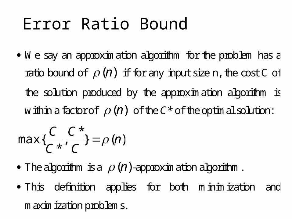
We say an approximation algorithm for the problem has a

ratio bound of )(n if for any input size n, the cost C of

the solution produced by the approximation algorithm is

within a factor of )(n of the C* of the optimal solution:

)(}*

,*

max{ nC

CCC

The algorithm is a )(n -approximation algorithm.

This definition applies for both minimization and

maximization problems.

Error Ratio Bound

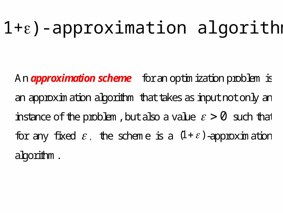
An approximation scheme for an optimization problem is

an approximation algorithm that takes as input not only an

instance of the problem, but also a value 0 such that

for any fixed , the scheme is a )1( -approximation

algorithm.

(1+)-approximation algorithm

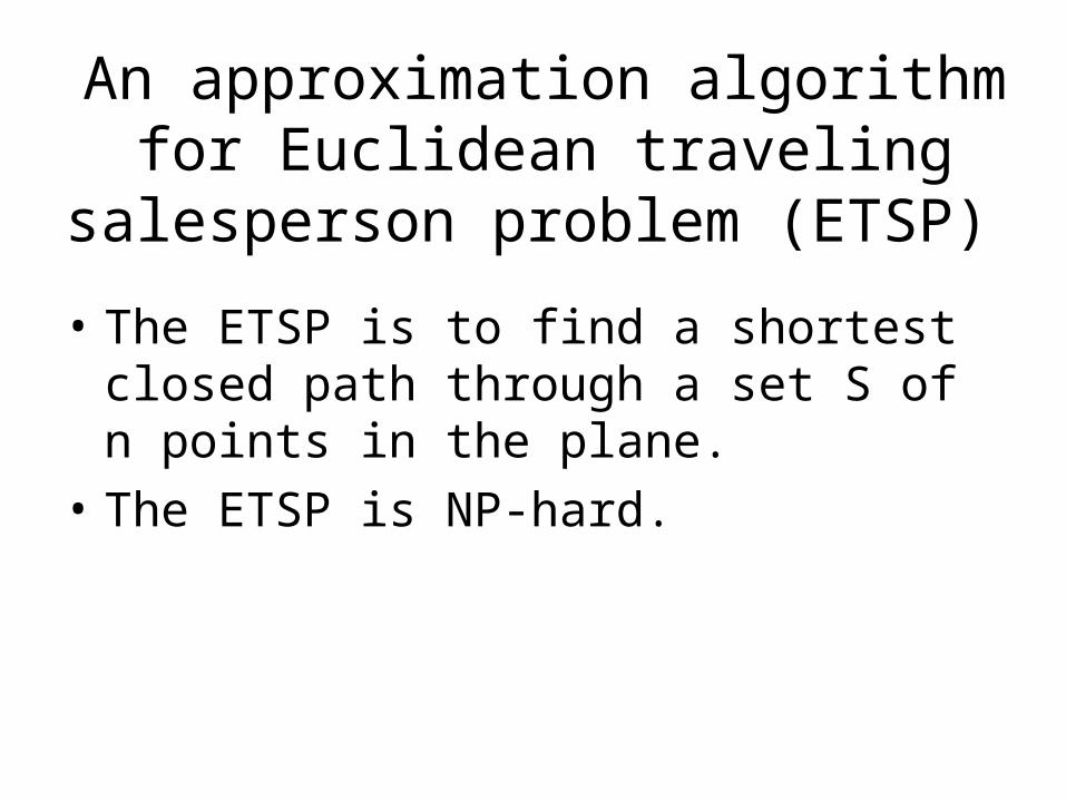
An approximation algorithm for Euclidean traveling salesperson

problem (ETSP)

• The ETSP is to find a shortest closed path through a set S of n points in the plane.

• The ETSP is NP-hard.

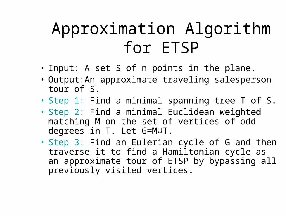
Approximation Algorithm for ETSP

• Input: A set S of n points in the plane.• Output:An approximate traveling salesperson tour

of S.• Step 1: Find a minimal spanning tree T of S.• Step 2: Find a minimal Euclidean weighted

matching M on the set of vertices of odd degrees in T. Let G=M∪T.

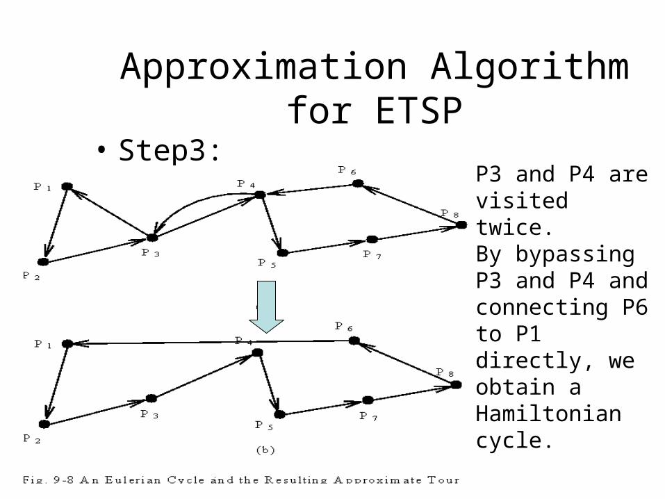
• Step 3: Find an Eulerian cycle of G and then traverse it to find a Hamiltonian cycle as an approximate tour of ETSP by bypassing all previously visited vertices.

Eulerian Cycle

• An Eulerian path (Eulerian trail, Euler walk) in a graph is a path that uses each edge precisely once. If such a path exists, the graph is called traversable.

• An Eulerian cycle (Eulerian circuit, Euler tour) in a graph is a cycle with uses each edge precisely once. If such a cycle exists, the graph is called Eulerian.

• L. Euler showed that an Eulerian cycle exists if and only if all vertices in the graph are of even degree and all edges are contained in the same component.

• L. Euler also showed an Eulerian path exists, if and only if at most two vertices in the graph are of odd degree and all edges are contained in the same component.

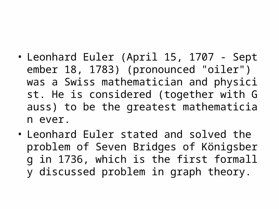
• Leonhard Euler (April 15, 1707 - September 18, 1783) (pronounced "oiler") was a Swiss mathematician and physicist. He is considered (together with Gauss) to be the greatest mathematician ever.

• Leonhard Euler stated and solved the problem of Seven Bridges of Königsberg in 1736, which is the first formally discussed problem in graph theory.

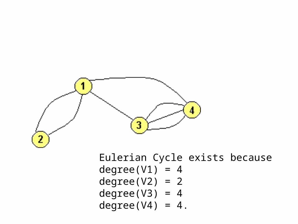
Eulerian Cycle exists becausedegree(V1) = 4degree(V2) = 2degree(V3) = 4degree(V4) = 4.

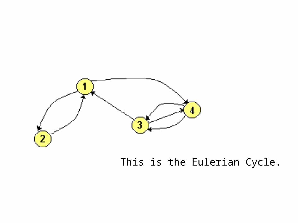
This is the Eulerian Cycle.

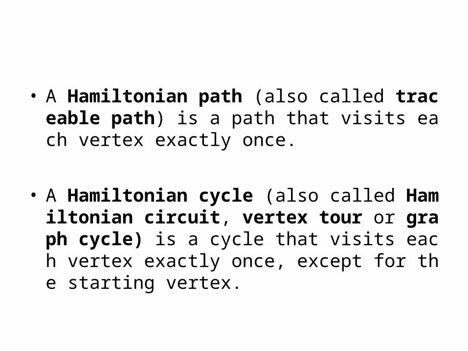
• A Hamiltonian path (also called traceable path) is a path that visits each vertex exactly once.

• A Hamiltonian cycle (also called Hamiltonian circuit, vertex tour or graph cycle) is a cycle that visits each vertex exactly once, except for the starting vertex.

Minimal Euclidean Weighted Matching Problem

• Given a set of points in the plane, the minimal Euclidean weighted matching problem is to join the points in pairs by line segments such that the total length is minimum.

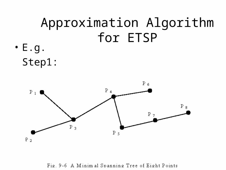
Approximation Algorithm for ETSP• E.g.

Step1:

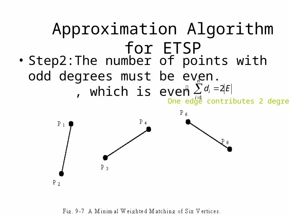
Approximation Algorithm for ETSP• Step2:The number of points with odd

degrees must be even. , which is even

n

ii Ed

1

2

One edge contributes 2 degrees

Approximation Algorithm for ETSP

• Step3:P3 and P4 are visited twice.By bypassing P3 and P4 and connecting P6 to P1 directly, we obtain a Hamiltonian cycle.

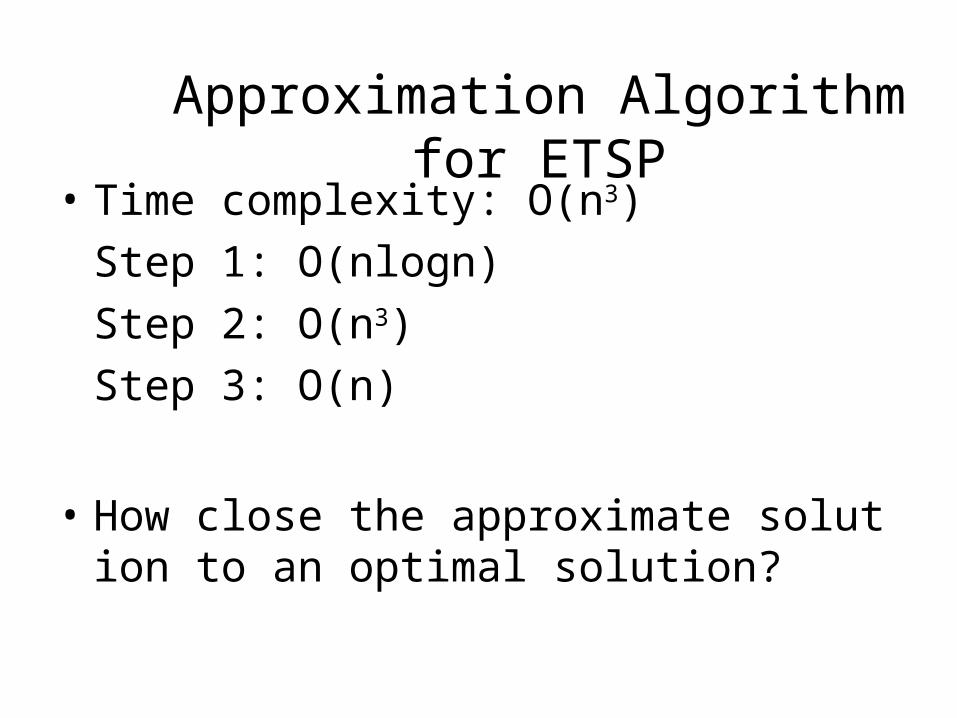
Approximation Algorithm for ETSP• Time complexity: O(n3)

Step 1: O(nlogn)

Step 2: O(n3)

Step 3: O(n)

• How close the approximate solution to an optimal solution?

How good is the solution ?

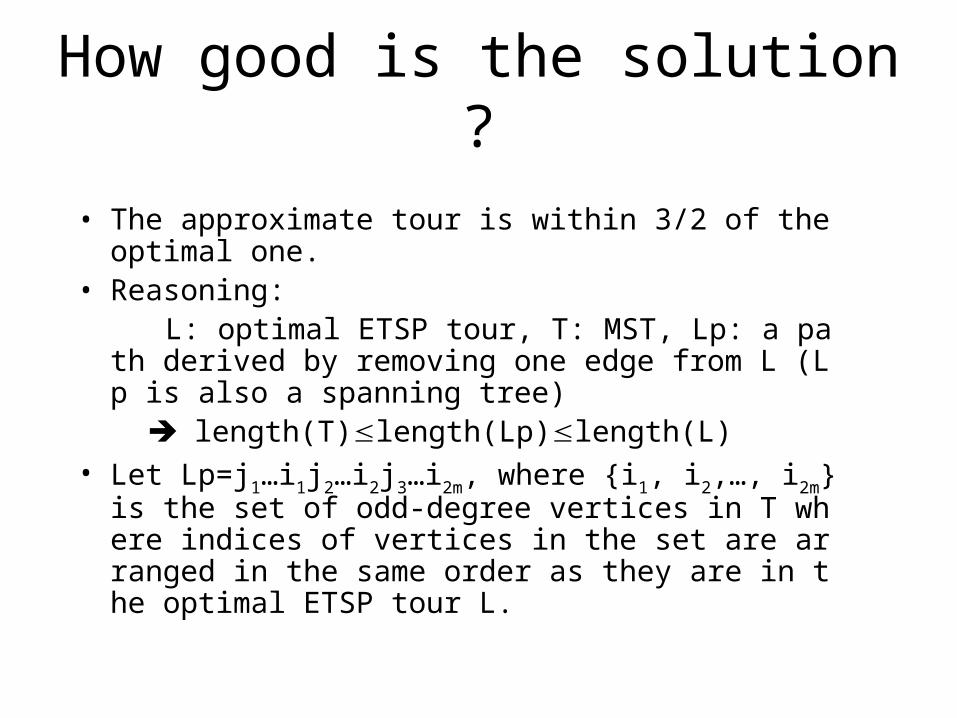
• The approximate tour is within 3/2 of the optimal one.

• Reasoning: L: optimal ETSP tour, T: MST, Lp: a path derived b

y removing one edge from L (Lp is also a spanning tree)

length(T)length(Lp)length(L)• Let Lp=j1…i1j2…i2j3…i2m, where {i1, i2,…, i2m} is the se

t of odd-degree vertices in T where indices of vertices in the set are arranged in the same order as they are in the optimal ETSP tour L.

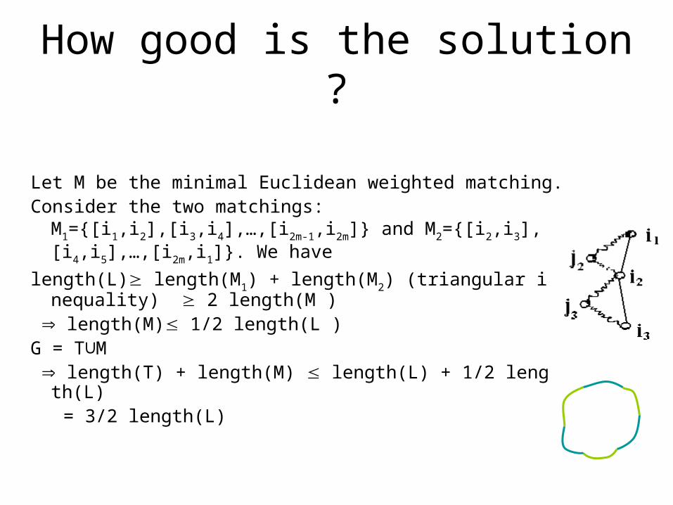
How good is the solution ?

Let M be the minimal Euclidean weighted matching.Consider the two matchings:

M1={[i1,i2],[i3,i4],…,[i2m-1,i2m]} and M2={[i2,i3],[i4,i5],…,[i2m,i1]}. We have

length(L) length(M1) + length(M2) (triangular inequality) 2 length(M )

length(M) 1/2 length(L )G = T∪M length(T) + length(M) length(L) + 1/2 length(L) = 3/2 length(L)

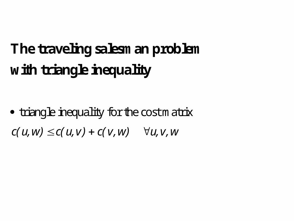
The traveling salesman problem

with triangle inequality

triangle inequality for the cost matrix

c u w c u v c v w u v w( , ) ( , ) ( , ) , ,

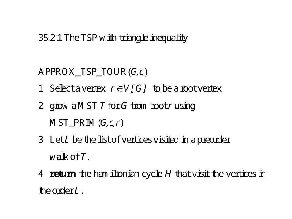
35.2.1 The TSP with triangle inequality

APPROX_TSP_TOUR(G,c)

1 Select a vertex r V G [ ] to be a root vertex

2 grow a MST T for G from root r using

MST_PRIM(G,c,r)

3 Let L be the list of vertices visited in a preorder

walk of T.

4 return the hamiltonian cycle H that visit the vertices in

the order L.

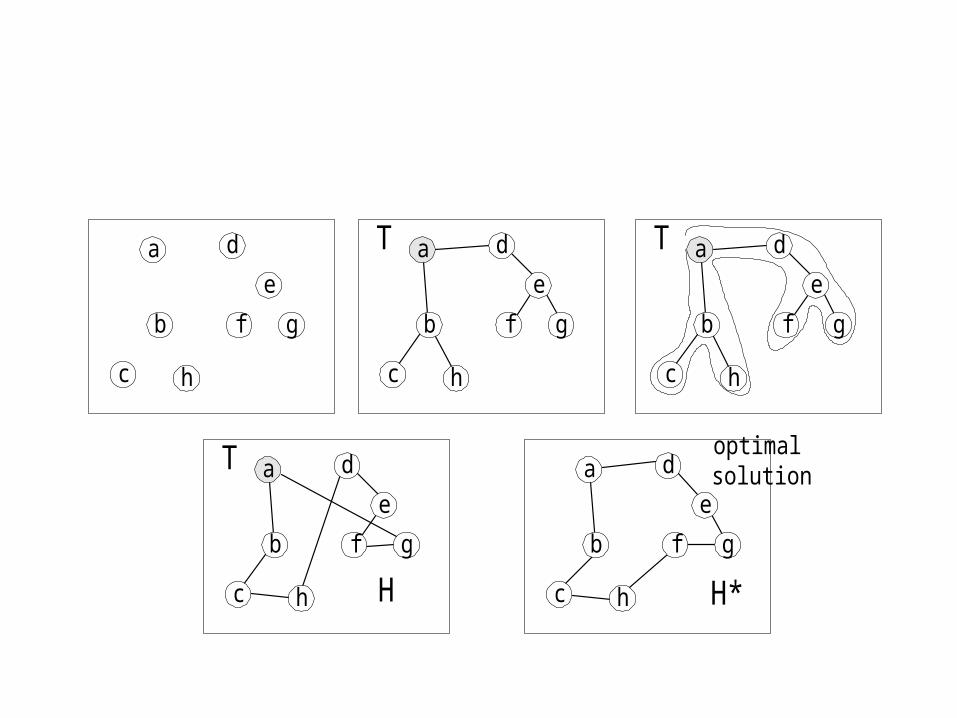
a d

f

c

b

e

g

h

a d

f

c

b

e

g

h

T a d

f

c

b

e

g

h

T

T a d

f

c

b

e

g

h

optimalsolutiona d

f

c

b

e

g

hH H*

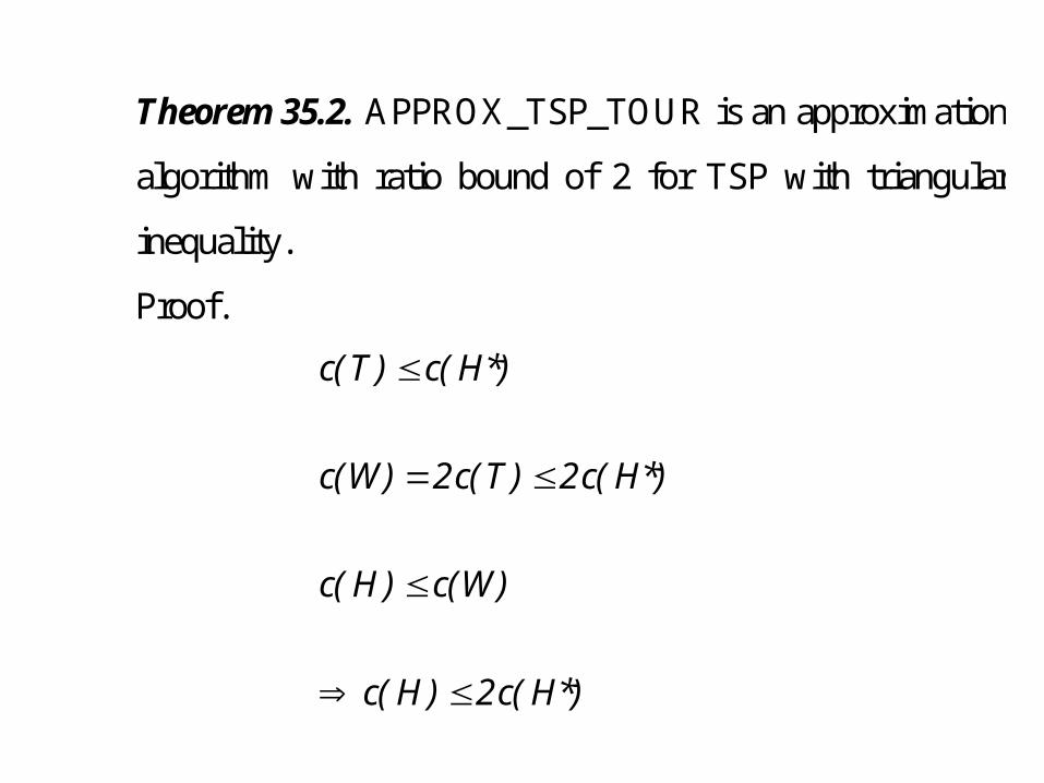
Theorem 35.2. APPROX_TSP_TOUR is an approximation

algorithm with ratio bound of 2 for TSP with triangular

inequality.

Proof.

c T c H

c W c T c H

c H c W

c H c H

( ) ( *)

( ) ( ) ( *)

( ) ( )

( ) ( *)

2 2

2

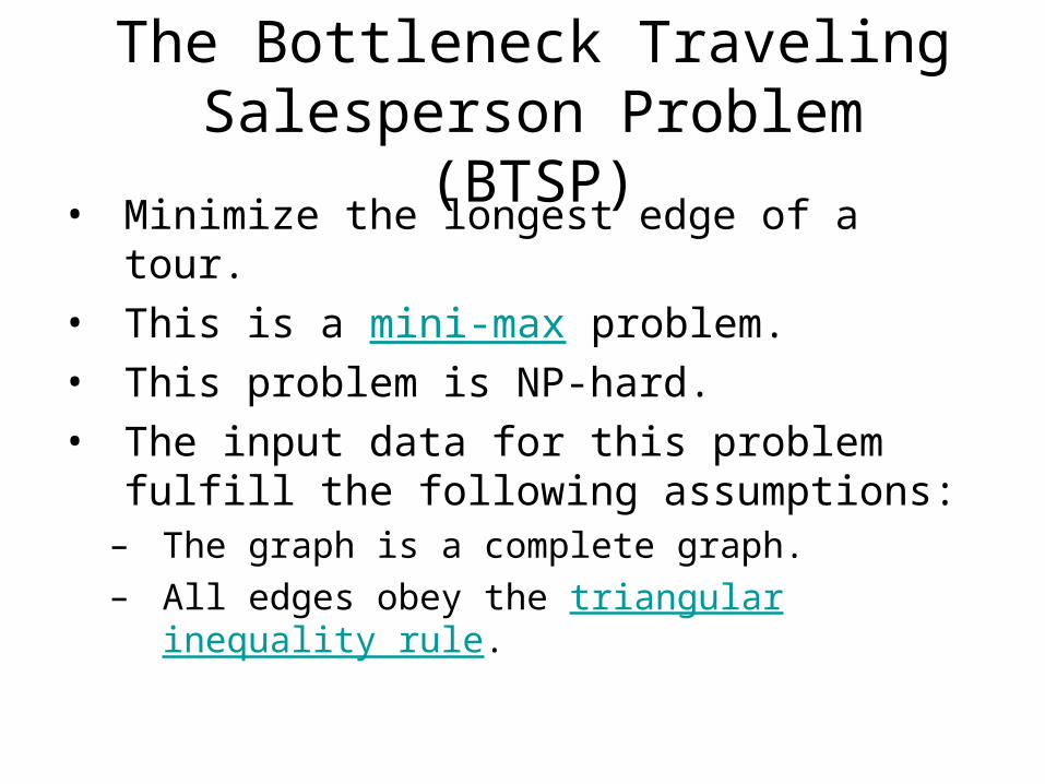
The Bottleneck Traveling Salesperson Problem (BTSP)

• Minimize the longest edge of a tour.

• This is a mini-max problem.

• This problem is NP-hard.

• The input data for this problem fulfill the following assumptions:

– The graph is a complete graph.– All edges obey the triangular inequality rule.

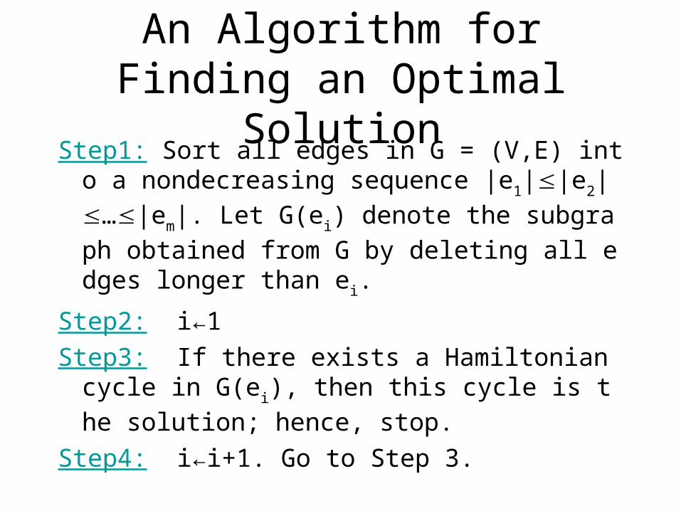
An Algorithm for Finding an Optimal Solution

Step1: Sort all edges in G = (V,E) into a nondecreasing sequence |e1||e2|…|em|. Let G(ei)

denote the subgraph obtained from G by deleting all edges longer than ei.

Step2: i←1

Step3: If there exists a Hamiltonian cycle in G(ei), then this cycle is the solution; hence, sto

p.

Step4: i←i+1. Go to Step 3.

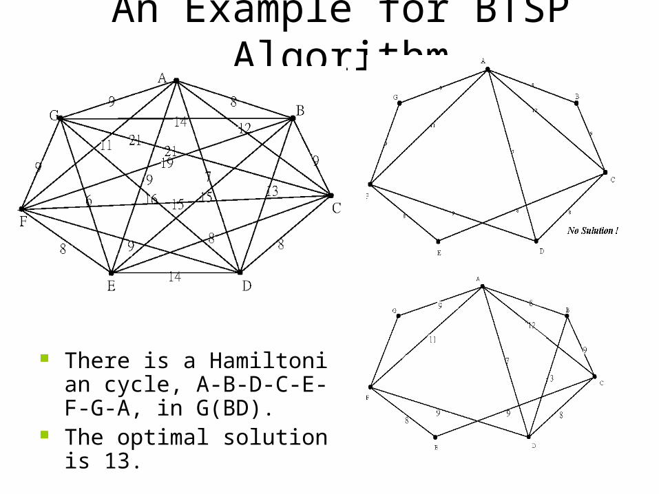
An Example for BTSP Algorithm

• e.g.

There is a Hamiltonian cycle, A-B-D-C-E-F-G-A, in G(BD).

The optimal solution is 13.

Time complexity of the algorithm

• The Hamiltonian cycle problem is NP-hard.

• The algorithm cannot be a polynomial one.

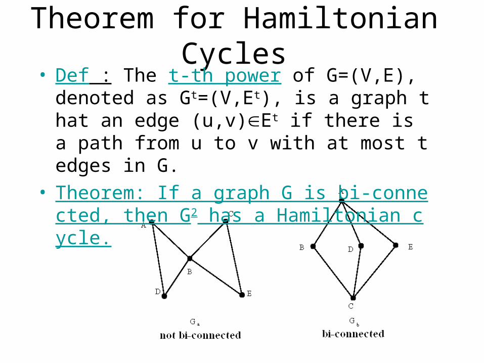
Theorem for Hamiltonian Cycles• Def : The t-th power of G=(V,E), denoted as

Gt=(V,Et), is a graph that an edge (u,v)Et if there is a path from u to v with at most t edges in G.

• Theorem: If a graph G is bi-connected, then G2 has a Hamiltonian cycle.

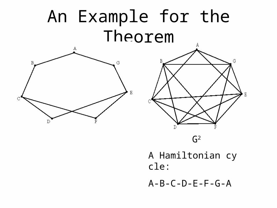
An Example for the Theorem

A Hamiltonian cycle:

A-B-C-D-E-F-G-A

G2

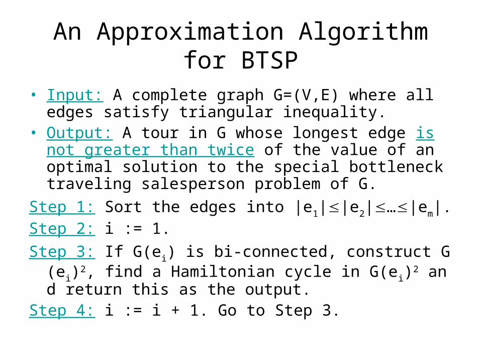
An Approximation Algorithm for BTSP

• Input: A complete graph G=(V,E) where all edges satisfy triangular inequality.

• Output: A tour in G whose longest edge is not greater than twice of the value of an optimal solution to the special bottleneck traveling salesperson problem of G.

Step 1: Sort the edges into |e1||e2|…|em|.Step 2: i := 1.

Step 3: If G(ei) is bi-connected, construct G(ei)2, find a Hami

ltonian cycle in G(ei)2 and return this as the output.

Step 4: i := i + 1. Go to Step 3.

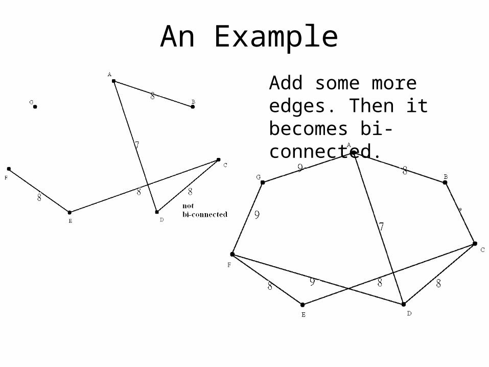
An Example

Add some more edges. Then it becomes bi-connected.

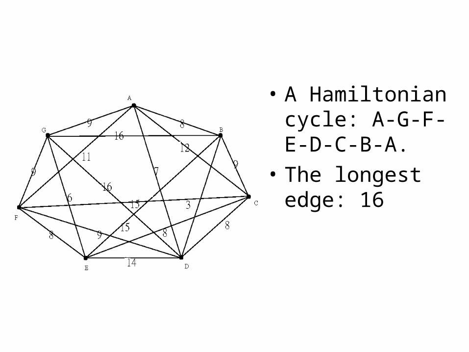
• A Hamiltonian cycle: A-G-F-E-D-C-B-A.

• The longest edge: 16

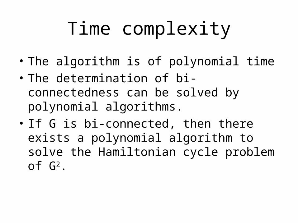
Time complexity

• The algorithm is of polynomial time

• The determination of bi-connectedness can be solved by polynomial algorithms.

• If G is bi-connected, then there exists a polynomial algorithm to solve the Hamiltonian cycle problem of G2.

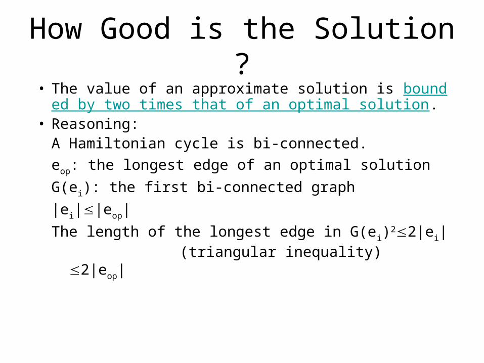
How Good is the Solution ?• The value of an approximate solution is bounded

by two times that of an optimal solution. • Reasoning:

A Hamiltonian cycle is bi-connected.

eop: the longest edge of an optimal solution

G(ei): the first bi-connected graph

|ei||eop|

The length of the longest edge in G(ei)22|ei|

(triangular inequality) 2|eop|