Approximation Algorithms for Product Framing and Pricingvt2196/MPR_ORSubmission.pdf ·...
39
Submitted to Operations Research manuscript (Please, provide the manuscript number!) Authors are encouraged to submit new papers to INFORMS journals by means of a style file template, which includes the journal title. However, use of a template does not certify that the paper has been accepted for publication in the named jour- nal. INFORMS journal templates are for the exclusive purpose of submitting to an INFORMS journal and should not be used to distribute the papers in print or online or to submit the papers to another publication. Approximation Algorithms for Product Framing and Pricing Guillermo Gallego, Anran Li, Van-Anh Truong, Xinshang Wang Department of Industrial Engineering and Operations Research, Columbia University, New York, NY, USA, [email protected],[email protected], [email protected],[email protected] We propose one of the first models of “product framing” and pricing. Product framing refers to the way consumer choice is influenced by how the products are framed, or displayed. We present a model where a set of products are displayed, or framed, into a set of virtual web pages. We assume that consumers consider only products in the top pages, with different consumers willing to see a different number of pages. Consumers select a product, if any, from these pages following a general choice model. We show that the product framing problem is NP-hard. We derive algorithms with guaranteed performance relative to an optimal algorithm under reasonable assumptions. Our algorithms are fast, easy to implement, and dominate the best known performance bounds. We also present structural results for pricing under framing effects. At optimality, products are sorted in descending order of quality, and prices are shown to be page dependent, with higher prices associated with products on pages seen by fewer consumers, so products in the first page are of the highest quality and have the lowest prices. 1. Introduction In this paper, we propose one of the first models of product framing and pricing. Framing refers to the way in which the choice among available alternatives is influenced by how the alternatives are framed, or displayed (Tversky and Kahneman 1986). For example, empirical works by Agarwal, Hosanagar and Smith (2009) and Ghose and Yang (2009) in online advertising show that ads that are placed higher on a webpage attract more clicks from consumers. Johnson, Moe, Fader, Bellman and Lohse (2004) examine the average number of websites, sorted by product categories, that are 1
Transcript of Approximation Algorithms for Product Framing and Pricingvt2196/MPR_ORSubmission.pdf ·...
Submitted to Operations Researchmanuscript (Please, provide the manuscript number!)
Authors are encouraged to submit new papers to INFORMS journals by means ofa style file template, which includes the journal title. However, use of a templatedoes not certify that the paper has been accepted for publication in the named jour-nal. INFORMS journal templates are for the exclusive purpose of submitting to anINFORMS journal and should not be used to distribute the papers in print or onlineor to submit the papers to another publication.
Approximation Algorithms for Product Framing andPricing
Guillermo Gallego, Anran Li, Van-Anh Truong, Xinshang WangDepartment of Industrial Engineering and Operations Research, Columbia University, New York, NY, USA,
[email protected],[email protected], [email protected],[email protected]
We propose one of the first models of “product framing” and pricing. Product framing refers to the way
consumer choice is influenced by how the products are framed, or displayed. We present a model where a set
of products are displayed, or framed, into a set of virtual web pages. We assume that consumers consider only
products in the top pages, with different consumers willing to see a different number of pages. Consumers
select a product, if any, from these pages following a general choice model. We show that the product framing
problem is NP-hard. We derive algorithms with guaranteed performance relative to an optimal algorithm
under reasonable assumptions. Our algorithms are fast, easy to implement, and dominate the best known
performance bounds. We also present structural results for pricing under framing effects. At optimality,
products are sorted in descending order of quality, and prices are shown to be page dependent, with higher
prices associated with products on pages seen by fewer consumers, so products in the first page are of the
highest quality and have the lowest prices.
1. Introduction
In this paper, we propose one of the first models of product framing and pricing. Framing refers to
the way in which the choice among available alternatives is influenced by how the alternatives are
framed, or displayed (Tversky and Kahneman 1986). For example, empirical works by Agarwal,
Hosanagar and Smith (2009) and Ghose and Yang (2009) in online advertising show that ads that
are placed higher on a webpage attract more clicks from consumers. Johnson, Moe, Fader, Bellman
and Lohse (2004) examine the average number of websites, sorted by product categories, that are
1

Author: Article Short Title2 Article submitted to Operations Research; manuscript no. (Please, provide the manuscript number!)
actively visited by households each month. They observe that in a typical search session, consumers
search from fewer than two stores. Their data shows that 70% of the CD shoppers, 70% of the
book shoppers, and 42% of travel shoppers are loyal to just one site. Brynjolfsson, Dick, and Smith
(2010) find on a website that catalogs price and product information from multiple retailers, that
only 9% of users select offers that are listed beyond the first page. In related search contexts, Baye,
Gatti, Kattuman and Morgan (2009) have found that a consumer’s likelihood of visiting a firm
and purchasing from it is strongly related to the order in which the firm is listed on a webpage by
a search engine. They find that a firm receives about 17% fewer clicks for every competitor listed
above it on the screen, all other things being equal.
This well-documented framing effect is a natural outcome of the cognitive burden of processing
larger and larger assortments. During online shopping, it is cognitively harder for a typical consumer
to visit sellers who are listed at the bottom of a web page, before or in addition to visiting those
who are listed at the top (Animesh, Viswanathan and Agarwal 2011). In the context of online
retailing, it has been observed that consumers’ attention to a display decreases exponentially with
the display’s distance to the top (Feng, Bhargava, and Pennock 2007). Thus, positioning a brand
or product at a top position on a listing can improve both consumer attention to the brand, and
consequently, consumer selection of the brand (Chandon, Hutchinson, Bradlow, and Young 2009).
1.1. Model overview
Despite substantial evidence suggesting the impact of framing on consumers’ choice outcome, there
are very few models that have attempted to capture these effects. In this paper, we introduce one
of the first models for product framing and the first one for pricing that account explicitly for these
effects.
We base our model on the notion of consideration set. A consideration set is a set of products
over which a consumer will make utility comparisons before arriving at the final purchase decision.
Consideration sets have gained considerable acceptance since their introduction in the seminal
work of Howard and Sheth (1969). A widely used approach to modeling choice in psychology and
Author: Article Short TitleArticle submitted to Operations Research; manuscript no. (Please, provide the manuscript number!) 3
marketing is to assume that a consumer will first form a consideration set. Then he will choose
from among the alternatives in the set. Consideration sets explain, behaviorally, consumers’ limited
ability to process or acquire information (Manrai and Andrews 1998). Methodologically, it has
been shown that ignoring consideration sets may lead to biased parameter estimates (Chiang, Chib
and Narasimhan 1999), whereas including consideration sets improve the predictability of choice
models (Hauser and Gaskin 1984, Silk and Urban 1978). As an example, Hauser (1978) finds that
a disproportionate 78% of the explainable uncertainty in consumer choices can be accounted for by
consideration sets, whereas the Multinomial Logit Model (MNL) can only capture the remaining
22%.
We capture the effect of framing on the formation of consideration sets as follows. Products are
organized into virtual pages. Each page can hold a finite number, say p, of products. A consumer
will examine only the first X pages, where X is a random variable that may be personalized to
the consumer’s profile. The consumer forms a consideration set consisting of only products in the
examined pages. From this consideration set, the consumer makes a choice to purchase a product,
if any, according to a general choice model. Thus, products that are placed in earlier pages are
more likely to be considered, and therefore purchased, than those that are placed in later pages.
In addition, we capture two other effects that come into play after the consideration sets have
been formed. We call these effect location preference. Location preference works as follows. First,
given that a collection of pages enters into a consumer’s consideration set, products that are
displayed higher on a page are more likely to be chosen than those displayed lower on the same
page, all other factors being equal. Second, products that are listed in earlier pages are more likely
to be chosen than products that are listed in later pages, all other factors being equal. With location
preference, we require that the choice model be the MNL model. We capture the effect of location
on choice by using location-dependent preference weights, which we will describe in greater detail
in Section 7.
Given the above effects, we study two problems that are faced by an e-retailer who is managing
n different products in a particular product category. The retailer’s product framing problem is how

Author: Article Short Title4 Article submitted to Operations Research; manuscript no. (Please, provide the manuscript number!)
to determine an assortment and a distribution of the products in the assortment into the different
pages in order to maximize expected revenue. The retailer’s price framing problem looks into both
framing and pricing to maximize expected revenues.
1.2. Results and Implications for Brick-and-Mortar Retailers
Our contributions in this paper are the followings:
• We propose one of the first models of framing effects. Our model is more general than those
proposed earlier, allowing for a general choice model and a more general framing structure.
• We prove that the product framing problem is NP-hard, even when there are just 2 pages and
the choice model is the MNL model.
• We propose fast, easy-to-implement algorithms with worst-case performance guarantees. Our
algorithms are significantly simpler than existing algorithms and offer much better performance
bounds. The ease and simplicity of the algorithms mean that they can be personalized on-line for
each arriving consumer.
• We prove new structural results for pricing under framing effects. We show that given a
fixed placement of products, at optimality, each page is filled with products until all products are
displayed. All products on the same page have the same page-level price. When the ordering of
the products is endogenized, then higher quality products are given priority. This implies that the
optimal price is higher for less attractive products, which is contrary to the findings of Arbatskaya
(2007). They argue that sellers lower on a list will charge lower prices; thus, consumers with lower
search costs will search longer and obtain better deals. In contrast, our results show that consumers
with lower search costs will see less desirable products with higher prices.
We remark that our model, although tailored to e-commerce and virtual pages, can also be used
to model brick-and-mortar retailers, with a suitable interpretation of what consumers are willing
to look at. Some consumers, for example, would only look at the most prominent displays, while
others may enter the store and look at some isles or the rest of the store. Our location preference
model can also serve in brick-and-mortar settings to signify the value of having products at eye

Author: Article Short TitleArticle submitted to Operations Research; manuscript no. (Please, provide the manuscript number!) 5
level versus waist level, versus shoe level, and the value of end-of-isle locations. Our pricing results
also have implications for brick-and-mortar retailers. The most prominent displays should have the
highest quality products at the lowest prices.
1.3. Relation to assortment planning
Our paper falls within the literature on assortment planning, which is currently a very active area of
research. Assortment planning began with a stylized model introduced by van Ryzin and Mahajan
(1999). Van Ryzin and Mahajan (1999) show that under the MNL model, an optimal assortment
consists of a certain number of highest-utility products when the products are equally profitable.
When the products’ prices are given exogenously and the choice model is the MNL, Talluri and
van Ryzin (2004) prove that an optimal assortment includes a certain number of products with
the highest revenues.
The assortment-planning problem is easy to solve for the MNL model over a given consideration
set. Davis, Gallego and Topaloglu (2013) show that this problem can be formulated as a linear
program with totally unimodular constraints. Davis, Gallego and Topaloglu (2014) also propose
that under the nested logit (NL) model, the assortment-planning problem can be solved by a
linear program when the nest dissimilarity parameters of the choice model are less than one, and a
consumer always makes a purchase within the selected nest. Relaxing either of these assumptions
renders the problem NP-hard.
The assortment-planning problem over a single consideration set is NP-hard for general choice
models. Indeed, Bront et al. (2009) show that under the mixed multinomial logit (MMNL) choice
model, the assortment-planning problem with a fixed number of mixtures is NP-hard. Desir and
Goyal (2013) show that this problem is even NP-hard to approximate within factor O(n1−ε), for
any fixed ε > 0. They give approximation schemes that tradeoff running time with solution quality,
but the running time for their approach grows exponentially with the number of mixtures.
Assortment planning with search costs has been studied by a number of authors. Cachon (2005)
shows that ignoring consumer search will lead to less assortment variety, since in equilibrium, the

Author: Article Short Title6 Article submitted to Operations Research; manuscript no. (Please, provide the manuscript number!)
seller needs a larger assortment to attract more consumers. Sahin and Wang (2015) also study the
assortment-optimization problem with search costs. They assume consumers are homogeneous and
their search sequence is predetermined by all the products’ expected utilities, which are known.
A few papers have studied assortment planning with location effects, but ignoring consideration
sets. Davis, Gallego and Topaloglu (2013) model location effects by introducing location-dependent
item weights to the MNL model. The resulting assortment-optimization problem is polynomial
time solvable because of its totally unimodular constraints. Feldman and Topaloglu (2015) study
a model in which consumers choose products according to the MNL model, but consumers of
different types have different consideration sets, and the sets are fixed and nested. They devise a
fully polynomial-time approximation scheme for this problem.
To our knowledge, there are only two papers that model a framing-dependent formation of con-
sideration sets. Davis, Topaloglu and Williamson (2015) study a problem in which a firm must
sequentially add products to its assortment over time, thereby monotonically increasing consumers’
consideration sets. They provide an algorithm with constant relative performance. The decision
space for this problem is much more constrained than ours and the application context is very
specific. Aouad and Segev (2016) consider a special case of our model, where the number of prod-
ucts that can be displayed on each page is one and the choice model is the MNL. Their require
more restrictive assumptions than ours, their algorithms are more complex, and their bounds are
significantly weaker.
1.4. Relation to assortment pricing
Our work also falls within the area of assortment pricing. Hanson and Martin (1996) are among
the first to notice that the expected revenue function fails to be concave in pricing problems, even
under the MNL model. Song and Xue (2007) show that by changing the decision variables and
reformulating the expected revenue as a concave function with respect to the market shares. Under
the MNL model with uniform price-sensitivity parameter, the markup, defined as price minus cost,
has been shown to be constant across all products at optimality (Anderson, de Palma and Thisse

Author: Article Short TitleArticle submitted to Operations Research; manuscript no. (Please, provide the manuscript number!) 7
1992, Hopp and Xu 2005, and Gallego and Stefanescu 2011). By assuming that the price sensitivities
of the products are constant within each nest and the nest dissimilarity parameters are restricted to
the unit interval, Li and Huh (2011) extend the concavity result to the NL model. Gallego and Wang
(2014) consider the general NL model with product-differentiated price-sensitivity parameters and
arbitrary nest coefficients. They find that the adjusted nest-level markup is also constant across
all the nests.
We extend the assortment-pricing literature to model framing effects. Under the MNL revenue
(profit) maximization model, we find that the constant price (markup) property still holds at the
page level. We also show that the price is higher for less attractive products, which is contrary to
the findings of Arbatskaya (2007).
2. Product-Framing Problem
Consider n products. Product i has revenue ri, i ∈N = {1, . . . , n}. The revenue can be the profit
contribution net of costs in some applications. Products are organized into virtual pages. Each
page can hold up to p products. Potentially all of the products may be offered, but offering all of
the products is not a hard requirement. Consumers who arrive at the system have consideration
sets that are governed by a random variable X taking values in a set M that consists of all the
positive integers, or is of the form {1, . . . ,m} for some positive integer m. Let λ(x) = P[X = x], and
Λ(x) = P[X ≥ x] for all x∈M. A consumer who draws X = x∈M has consideration set {1, . . . , x}.
From this consideration set, the consumer purchases at most one product according to a general
choice model.
The product-framing problem is to distribute the products among the pages to maximize the
expected revenue that can be obtained from an arriving consumer. We assume that we do not know
the number of pages that a consumer is willing to view when he arrives into the system. We assume,
however, that the distribution of X is known and is independent of the framing of the products.
Knowledge of X can be acquired from observing click data and by computing the frequency of
consumers who examine x∈M pages. By the law of large numbers, these frequencies converge to
Author: Article Short Title8 Article submitted to Operations Research; manuscript no. (Please, provide the manuscript number!)
the probability distribution of X. We call this multi-page assortment-optimization problem, the
product-framing problem. Although we will refer to a single random variable X, it is easy to see
that X can be personalized to heterogeneous consumer types based on available information about
the distribution of pages they are willing to see. Information that may change the distribution of
X includes, but is not limited to, prior purchases, zip code, age, and gender.
The product-framing problem can be formulated in terms of the decision variables yij ∈ {0,1}, i∈
N , j ∈M, where yij = 1 if item i is displayed on page j and is zero otherwise. Let P (i,S) denote
the purchase probability of item i when the consideration set is S ⊆N , with P (i,S) = 0 if i 6∈ S.
The formulation in terms of the variables yij is given by
OPT =maxyij
∑x∈M
λ(x)n∑i=1
riP (i,{k ∈N :x∑l=1
ykl = 1})
s.t.∑j∈M
yij ≤ 1, ∀i∈N
n∑i=1
yij ≤ p, ∀j ∈M
yij ∈ {0,1}, ∀i∈N , j ∈M.
(1)
We will show that problem (1) is NP-hard. Therefore, to derive performance bounds for our
algorithms, we will first find an upper bound of (1), which can be easily computed.
3. Upper Bound on Optimal Revenue for Product Framing
Consider the following assortment-optimization problem, which constrains the number of products
in an assortment to be at most c.
G(c) = maxS⊆N
∑i∈S
riP (i,S)
s.t. |S| ≤ c.
(2)
Let R(x) =G(x · p) be the optimal expected revenue from consumers who see x ∈M pages. Let
S(x)⊂N be an optimal solution associated with problem R(x). If we had the luxury of knowing

Author: Article Short TitleArticle submitted to Operations Research; manuscript no. (Please, provide the manuscript number!) 9
the number of pages x ∈M upon the arrival of a consumer, we would offer him assortment S(x),
and would earn expected revenue
E[R(X)] =∑x∈M
λ(x)R(x). (3)
The following result shows that this E[R(X)] is an upper bound on the expected value V OPT of
OPT .
Theorem 1. E[R(X)]≥ V OPT .
Proof. Suppose y∗ is an optimal solution to (1). We must have, for any x∈M,
R(x)≥n∑i=1
riP (i,{k ∈N :x∑l=1
y∗kl = 1})
=⇒∑x∈M
λ(x)R(x)≥ V OPT .
�
4. Hardness of Framing Problem
We show that problem (1) is NP-hard even in the special case that m= 2 and the choice model is
the MNL model. We do this by reducing the well-known 2-PARTITION problem to a special case
of our model. The 2-PARTITION problem is defined as follows
Definition 1 (2-PARTITION). Given a set of n non-negative numbers w1,w2, ...,wn, determine
whether there is a set S ⊆ {1,2, ..., n} such that∑
i∈S wi =∑
i 6∈S wi.
Our reduction works as follows. Starting with any instance of 2-PARTITION, we design a sequence
of instances of problem (1). We show that the sequence of solutions to the continuous relaxation
of these problems converge to a solution of the 2-PARTITION problem.
Theorem 2. Problem (1) is NP-hard even when the choice model is MNL.

Author: Article Short Title10 Article submitted to Operations Research; manuscript no. (Please, provide the manuscript number!)
5. Assumptions for Analysis of Algorithms
Given that the product framing problem is NP-hard, one of our goals will be to propose algo-
rithms with guaranteed performance ratios relative to OPT . Towards this goal, we will make three
innocuous assumptions:
Assumption 1.
R(x)/x is decreasing in x∈M.
Assumption 2. In polynomial time, we can obtain a solution with expected revenue G(c) to prob-
lem (2) such that G(c)≥ (1− ε)G(c) for some constant ε∈ (0,1].
Assumption 3. X has increasing failure rate (IFR) distribution.
Assumption 1 holds very generally. Indeed, Davis, Topaloglu and Williamson (2015) have shown
that if the choice model P (i,S) satisfies
P (i,S)≥ P (i, T ) for all i∈ S, and S ⊆ T ⊆N , (4)
then Assumption 1 holds. Notice that condition (4) holds for all random utility models. Assump-
tion 2 states that we can approximately solve the capacity-constrained problem (2) within a
constant approximation ratio. For the MNL and Nested Logit models, the capacity-constrained
problem can be solved exactly in polynomial time (ε = 0) (Gallego and Topaloglu 2014 ). The
Mixed Multinomial Logit model with a constant number of mixtures can also be solved within any
given error ε > 0 in polynomial time (Mittal and Schulz 2013, Desir and Goyal 2013). For ease of
exposition, in the rest of the paper we will just assume that ε= 0, but all of our algorithms and
bounds can be easily extended to the case of ε > 0 by replacing the revenue function R(x) with an
approximate value, and scaling the corresponding bound by (1− ε). Let h(x) = λ(x)
Λ(x)for all x ∈M
for which Λ(x)> 0. Assumption 3 is equivalent to h(x) increasing in x∈M. Assumption 3 implies
that the probability that a consumer will view the next page is decreasing in the number of pages
he or she has viewed.
Author: Article Short TitleArticle submitted to Operations Research; manuscript no. (Please, provide the manuscript number!) 11
The function R(x) is in general not concave, so we will not assume concavity except where noted.
We now briefly investigate conditions for the concavity of R(x) under the MNL. We will obtain
stronger bounds under the assumption that R(x) is concave. We remark that these stronger bounds
do not assume an MNL choice model.
Let V (x) =∑
j∈S(x) vj be the sum of the attraction values of the products in S(x) when the
choice model is MNL. A sufficient condition for R(x) to be concave under the MNL is given by the
following proposition.
Proposition 1. If the choice model is MNL and V (x) is increasing, then R(x) is concave.
A sufficient condition for this property, in the profit maximization MNL model, is that the net
profit contribution rj is ordered the same way as the attractiveness vj. For the MNL, prices are
typically set at pj = cj + θ resulting in net profit contributions equal to rj = θ. In this case we get
trivially rj and vj = exp(aj −β(cj + θ)) in the same order after sorting the products in decreasing
order of vj. The same is true if the “utility at cost” aj − βcj is in the same order of the quality
component aj and prices are quality-consistent, so higher quality implies higher prices. Even in
the absence of these reasonable conditions, it is quite likely that V (x) is increasing in x when p is
large as then S(x) includes p more products than S(x− 1), and it is unlikely that adding so many
products would result in a decrease in value, i.e., V (x)< V (x− 1), or equivalently, an increase in
the probability that the customer would not make a purchase. In other words, it is unlikely that
the probability of sale is lower for a consumer willing to see one more page when the number of
products per page is large.
Since any random utility model can be approximated by a mixture of MNLs, our result for
the MNL has implications for the mixture of MNL, and therefore for any random utility model.
Indeed, if S(x) is the optimal set for the mixture model for customers willing to see x pages,
and Vk(x) =∑
j∈S(x) vkj is the sum of the attraction values for consumers of type k, and Vk(x) is
increasing in x for each k, then the revenue function for the mixture model is also concave. Of
course, for the mixture model this is a condition that is harder to verify because it is NP-hard to
find the sets S(x), x∈M.

Author: Article Short Title12 Article submitted to Operations Research; manuscript no. (Please, provide the manuscript number!)
6. Algorithms with Constant Performance Bounds for Product Framing
We now propose algorithms for problem (1), which have guaranteed constant performance ratio
relative to OPT under Assumptions 1, 2, and 3. Stronger bounds will be obtained when concavity
of R(x) is also assumed. All of our performance guarantees in this section are tight relative to the
upper bound (3) in the sense that our proofs exhibit a way to construct instances in which the
bounds are achieved by our algorithms.
Our first algorithms, called NEST, start by truncating the number of pages to an arbitrary
integer y, and by selecting an optimal assortment, say S(y), for the first y pages. Then they select
an optimal assortment for the first y− 1 pages, say S(y− 1), by looking only at the products in
S(y). This procedure continues until the content of all pages have been determined. With a little
bit abuse of notations, we let R(S) denote the expected revenue when a consumer considers all the
products in set S.
NEST(y) Algorithms:
• Let y be an integer and let S(y) be the set of products with revenue R(y). Without loss of
generality, we assume that |S(y)|> (y−1)p. In other words, a minimum of y pages are required to
hold all products in S(y). If this fails, then we can select a smaller value of y until this assumption
holds.
• For x= y− 1 down to 1, let S(x) = arg maxS⊂S(x+1), |S|=xp
R(S) and let R(x) =R(S(x)).
• Use any heuristic to fill in pages x> y such that the total expected revenue of products in the
first x> y pages is at least R(y). As a default, we can leave pages x> y blank.
By Assumption 1, R(x)/x≥ R(y)/y=R(y)/y.
6.1. Constant bound with IFR Assumption
Let NEST =NEST (y) be an algorithm in the above class with
y= max arg maxx∈M
R(x)
xE[min(X,x)].
We will show that NEST achieves at least 6/π2 of the optimal expected revenue.
Author: Article Short TitleArticle submitted to Operations Research; manuscript no. (Please, provide the manuscript number!) 13
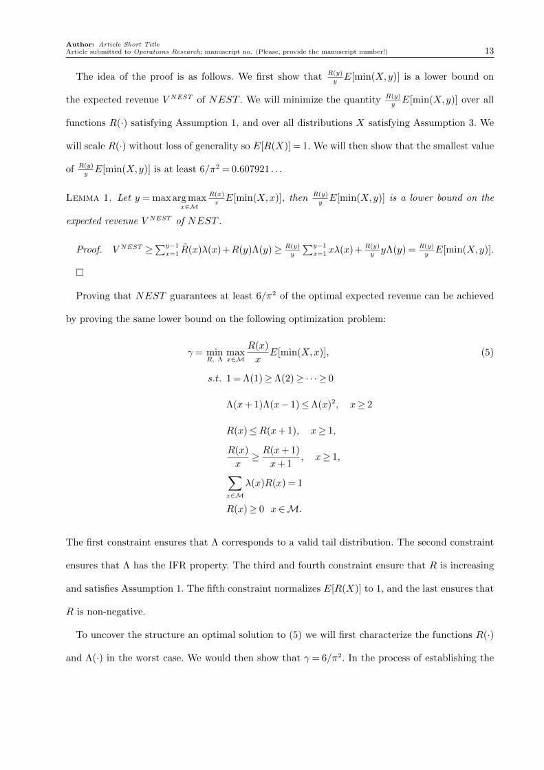
The idea of the proof is as follows. We first show that R(y)
yE[min(X,y)] is a lower bound on
the expected revenue V NEST of NEST . We will minimize the quantity R(y)
yE[min(X,y)] over all
functions R(·) satisfying Assumption 1, and over all distributions X satisfying Assumption 3. We
will scale R(·) without loss of generality so E[R(X)] = 1. We will then show that the smallest value
of R(y)
yE[min(X,y)] is at least 6/π2 = 0.607921 . . .
Lemma 1. Let y = maxarg maxx∈M
R(x)
xE[min(X,x)], then R(y)
yE[min(X,y)] is a lower bound on the
expected revenue V NEST of NEST .
Proof. V NEST ≥∑y−1
x=1 R(x)λ(x)+R(y)Λ(y)≥ R(y)
y
∑y−1
x=1 xλ(x)+ R(y)
yyΛ(y) = R(y)
yE[min(X,y)].
�
Proving that NEST guarantees at least 6/π2 of the optimal expected revenue can be achieved
by proving the same lower bound on the following optimization problem:
γ = minR, Λ
maxx∈M
R(x)
xE[min(X,x)], (5)
s.t. 1 = Λ(1)≥Λ(2)≥ · · · ≥ 0
Λ(x+ 1)Λ(x− 1)≤Λ(x)2, x≥ 2
R(x)≤R(x+ 1), x≥ 1,
R(x)
x≥ R(x+ 1)
x+ 1, x≥ 1,∑
x∈M
λ(x)R(x) = 1
R(x)≥ 0 x∈M.
The first constraint ensures that Λ corresponds to a valid tail distribution. The second constraint
ensures that Λ has the IFR property. The third and fourth constraint ensure that R is increasing
and satisfies Assumption 1. The fifth constraint normalizes E[R(X)] to 1, and the last ensures that
R is non-negative.
To uncover the structure an optimal solution to (5) we will first characterize the functions R(·)
and Λ(·) in the worst case. We would then show that γ = 6/π2. In the process of establishing the

Author: Article Short Title14 Article submitted to Operations Research; manuscript no. (Please, provide the manuscript number!)
bounds, we will not use special notation, say γ∗,R∗(·) or Λ∗(·) to denote the optimal solution to
program (5). This comes at a small cost of ambiguity, but makes the exposition a bit cleaner.
Let y= maxarg maxx∈M
R(x)
xE[min(X,x)] and γ = R(y)
yE[min(X,y)]. We next show worst case struc-
ture for R(x) for all x∈M.
Lemma 2. R(x) = γ xE[min(X,x)]
for all x∈M.
The lemma implies that in the worst case, all values of x∈M are maximizers of R(x)
xE[min(X,x)].
Proof. We first show the sequence R(x)
xE[min(X,x)] cannot decrease. Suppose there is a small-
est x > 1 such that R(x−1)
x−1E[min(X,x − 1)] > R(x)
xE[min(X,x)], then we can increase the value
of R(x′) for x′ = x,x + 1, x + 2... such that R(x′) = R(x), and reduce the rest of R(x′)’s, while
maintaining the constraint E[R(X)] = 1. The rescaling is valid because R(x−1)
x−1E[min(X,x− 1)]>
R(x)
xE[min(X,x)] implies R(x−1)
x−1> R(x)
x. Consequently, Assumption 1 will not be violated. The pro-
posed adjustment contradicts the optimality of Problem (5) because it reduces γ. We now show
that the sequence R(x)
xE[min(X,x)] cannot increase either. Suppose there is a smallest x> 1 such
that R(x−1)
x−1E[min(X,x− 1)] < R(x)
xE[min(X,x)], then we can increase the value of R(x′) for all
x′ < x, and reduce R(x′), x′ ≥ x, while maintaining the constraint E[R(X)] = 1. The rescaling is
valid because R(x−1)
x−1E[min(X,x− 1)] < R(x)
xE[min(X,x)] implies R(x− 1) < R(x). Consequently,
the condition R(·) being increasing will not be violated. The proposed adjustment contradicts the
optimality of Problem (5) because it reduces γ. �
For R(x) of the form given by Lemma 2, we next show how γ depends on the distribution of X,
by using the fact that E[R(X)] = 1.
Theorem 3. Let Y be a random variable, independent of X, with the same distribution as X.
Then
1
γ= max
X,YE
[X
E[min(X,Y )|X]
]. (6)
Proof. By Lemma 2, R(x) = γ xE[min(Y,x)]
, where Y is a random variable with the same distribu-
tion as the worst case X. Then
1 =E[R(X)] = γ∑x∈M
x
E[min(Y,x)]λ(x) = γE
[X
E[min(X,Y )|X]
].
Author: Article Short TitleArticle submitted to Operations Research; manuscript no. (Please, provide the manuscript number!) 15
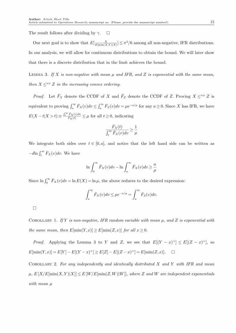
The result follows after dividing by γ. �
Our next goal is to show that E[ XE[min(X,Y )|X]
]≤ π2/6 among all non-negative, IFR distributions.
In our analysis, we will allow for continuous distributions to obtain the bound. We will later show
that there is a discrete distribution that in the limit achieves the bound.
Lemma 3. If X is non-negative with mean µ and IFR, and Z is exponential with the same mean,
then X ≤icx Z in the increasing convex ordering.
Proof. Let FX denote the CCDF of X and FZ denote the CCDF of Z. Proving X ≤icx Z is
equivalent to proving∫∞aFX(v)dv≤
∫∞aFZ(v)dv= µe−a/µ for any a≥ 0. Since X has IFR, we have
E(X − t|X > t)≡∫∞t FX (v)dv
FX (t)≤ µ for all t≥ 0, indicating
FX(t)∫∞tFX(v)dv
≥ 1
µ
We integrate both sides over t ∈ [0, a], and notice that the left hand side can be written as
−dln∫∞tFX(v)dv. We have
ln
∫ ∞0
FX(v)dv− ln
∫ ∞a
FX(v)dv≥ a
µ
Since ln∫∞
0FX(v)dv= lnE(X) = lnµ, the above reduces to the desired expression:∫ ∞
a
FX(v)dv≤ µe−a/µ =
∫ ∞a
FZ(v)dv.
�
Corollary 1. If Y is non-negative, IFR random variable with mean µ, and Z is exponential with
the same mean, then E[min(Y,x)]≥E[min(Z,x)] for all x≥ 0.
Proof. Applying the Lemma 3 to Y and Z, we see that E[(Y − x)+] ≤ E[(Z − x)+], so
E[min(Y,x)] =E[Y ]−E[(Y −x)+]≥E[Z]−E[(Z −x)+] =E[min(Z,x)]. �
Corollary 2. For any independently and identically distributed X and Y with IFR and mean
µ, E [X/E[min(X,Y )|X]]≤E [W/E[min(Z,W )|W ]], where Z and W are independent exponentials
with mean µ
Author: Article Short Title16 Article submitted to Operations Research; manuscript no. (Please, provide the manuscript number!)
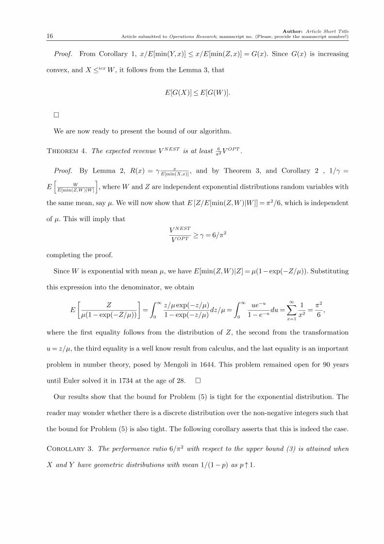
Proof. From Corollary 1, x/E[min(Y,x)] ≤ x/E[min(Z,x)] = G(x). Since G(x) is increasing
convex, and X ≤icxW , it follows from the Lemma 3, that
E[G(X)]≤E[G(W )].
�
We are now ready to present the bound of our algorithm.
Theorem 4. The expected revenue V NEST is at least 6π2V OPT .
Proof. By Lemma 2, R(x) = γ xE[min(X,x)]
, and by Theorem 3, and Corollary 2 , 1/γ =
E[
WE[min(Z,W )|W ]
], where W and Z are independent exponential distributions random variables with
the same mean, say µ. We will now show that E [Z/E[min(Z,W )|W ]] = π2/6, which is independent
of µ. This will imply that
V NEST
V OPT≥ γ = 6/π2
completing the proof.
Since W is exponential with mean µ, we have E[min(Z,W )|Z] = µ(1−exp(−Z/µ)). Substituting
this expression into the denominator, we obtain
E
[Z
µ(1− exp(−Z/µ))
]=
∫ ∞0
z/µ exp(−z/µ)
1− exp(−z/µ)dz/µ=
∫ ∞0
ue−u
1− e−udu=
∞∑x=1
1
x2=π2
6,
where the first equality follows from the distribution of Z, the second from the transformation
u= z/µ, the third equality is a well know result from calculus, and the last equality is an important
problem in number theory, posed by Mengoli in 1644. This problem remained open for 90 years
until Euler solved it in 1734 at the age of 28. �
Our results show that the bound for Problem (5) is tight for the exponential distribution. The
reader may wonder whether there is a discrete distribution over the non-negative integers such that
the bound for Problem (5) is also tight. The following corollary asserts that this is indeed the case.
Corollary 3. The performance ratio 6/π2 with respect to the upper bound (3) is attained when
X and Y have geometric distributions with mean 1/(1− p) as p ↑ 1.

Author: Article Short TitleArticle submitted to Operations Research; manuscript no. (Please, provide the manuscript number!) 17
Proof. Let X, Y be geometrically distributed with mean 11−p . That is, P [X = x] = P [Y = x] =
px−1(1− p). Then we can write
E
[X
E[min(X,Y )|X]
]=
∞∑y=1
py−1(1− p)2y
1− py.
For p < 1, we have
∞∑y=1
py−1(1− p)2y
1− py= (1− p)2
∞∑y=1
y
p
py
1− py
= (1− p)2
∞∑y=1
y
p
∞∑n=1
pyn
=(1− p)2
p
∞∑n=1
pn∞∑y=1
y(pn)y−1
=(1− p)2
p
∞∑n=1
pnd
dpn1
1− pn
=(1− p)2
p
∞∑n=1
pn1
(1− pn)2
=∞∑n=1
pn−1 (1− p)2
(1− pn)2.
The above series is an increasing function of p. It is maximized both locally and globally
at p = 1. To find the limit at p = 1, we use two applications of L’Hopital’s rule to obtain
limp→1
∑∞n=1 p
n−1 (1−p)2
(1−pn)2=∑∞
n=11n2
= π2
6. �
6.2. Constant bound under concavity of R(x)
If R(x) is concave, then we can improve the bound from 6/π2 = 0.607921 to (e− 1)/e= 0.63212.
Theorem 5. Assume that X has a continuous distribution, E[X] = µ is integral, and R(x) is
concave. Then under Assumptions 1, 2, and 3, the expected revenue V NEST is at least e−1eV OPT .
Proof As in the proof of Theorem 4,
V NEST ≥ maxy∈M
R(y)
yE[min(X,y)]
≥ R(µ)
µE[min(X,µ)]
≥ R(µ)
µµ(1− exp(−µ/µ))
= R(µ)(1− e−1).

Author: Article Short Title18 Article submitted to Operations Research; manuscript no. (Please, provide the manuscript number!)
where the first inequality results from ignoring the revenue of pages x> y, the second from selecting
µ, which is not necesarily optimal, and the third inequality follows from Corollary 2. From the
concavity of R(·), we have E[R(X)]≤R(µ), and consequently
V NEST
E[R(X)]≥ R(µ)(1− e−1)
R(µ)≥ e− 1
e.
�
For discrete distributions µ is unlikely to be an integer, so the bounds obtain for the concave case
should be considered a continuous approximation to the performance of the NESTED heuristic.
6.3. Improvement to the algorithms
We can refine the Nested Algorithms by extending the algorithms to pages beyond y. In particular,
let R(x) be the performance of the Nested Algorithms described above for all x≤ y. Set x= y+ 1
and solve the x-page problem subject to the constraint that the first y pages are composed of S(y).
Then select the products for page x= y+ 1 by solving the problem for page x among all products
in the complement of S(y). For higher values of x continue the procedure fixing the pages for all
z < x and selecting page x among the complement of the products used in pages 1, . . . , x− 1. Let
NEST + (y) be an algorithm in this improved class. When y is chosen as
y= maxarg maxx∈M
R(x)
xE[min(X,x)]
then we call NEST + (y) as NEST+. Note that NEST+ continues to have a worst-case perfor-
mance bound of 6π2
as we have proved in Section 6.1.
Corollary 4. If the capacitated assortment problem G(c) has the nested solution, i.e, S(1) ⊆
S(2)⊆ ...⊆ S(|N |), where S(c) is the optimal assortment for G(c), then NEST + (y) can return
an optimal frame.
In general, we can choose other values for y in NEST + (y). In the following theorem, we use
y = µ to obtain a lower bound bound for NEST+. To express our result more succinctly, we let
a=R(µ)/µ and b= (R(m)−R(µ))/(m−µ). Notice that a≥ b≥ 0.

Author: Article Short TitleArticle submitted to Operations Research; manuscript no. (Please, provide the manuscript number!) 19
Theorem 6. Assume that X has a continuous distribution, E[X] = µ is integral, R(x) is concave,
and the optimal assortment S(y)⊂ S(m). Then under Assumptions 1, 2, and 3,
V NEST+
V OPT≥ V NEST+(µ)
V OPT≥ e− 1
e+
b
ae.
Our worst case result for NEST (µ) makes the conservative assumption that b= 0.
7. Product Framing with Location Preferences
In online retail, consumers may be more likely to choose products that are displayed at the top
of search results, since consumers tend to associate high valuation with products displayed earlier
(Chandon, Hutchinson, Bradlow, and Young 2009). In this section, we augment our model to
capture the phenomenon that a consumer is more likely to buy an product that is displayed
earlier, even if the consumer has determined his consideration set. We model this phenomenon by
introducing the location-dependent preference weights to all products. We use νixq to denote the
preference weight of product i when this product is displayed at location q of page x. Without
loss of generality, we assume that there are as many possible locations as the number of products
so that we can offer all products at once. If the number of possible locations is smaller than the
number of products, then we can define additional locations with νixq = 0 for all i ∈ N for each
additional location (x, q), in which case, using one of these additional locations for a product is
equivalent to not displaying the product at all. To capture the product-framing decisions, we use
y = {yixq : i ∈N , x ∈M, q ∈ P} ∈ {0,1}n×m×p, where yixq = 1 if we offer product i in location q of
page x, otherwise yixq = 0. If the product offer decisions are given by y, then we obtain an expected
revenue of Rx(y) =∑n
i=1
∑xj=1
∑pq=1 yijqνijqri
1+∑n
i=1
∑xj=1
∑pq=1 yijqνijq
from consumers who only view the first x pages.
Recall that we can obtain the upper bound of the problem without location preference by
E(R(X))≡∑m
x=1 λ(x)R(x), where R(x)≡G(x · p) is the highest expected revenue from consumer
who is willing to view x pages. Under the MNL choice model, for the problem with location prefer-
ence, the problem G(x · p) is still polynomially solvable. This is because the problem is formulated
as
maxy
∑ni=1
∑xj=1
∑pq=1 yijqνijqri
1+∑n
i=1
∑xj=1
∑pq=1 yijqνijq
Author: Article Short Title20 Article submitted to Operations Research; manuscript no. (Please, provide the manuscript number!)
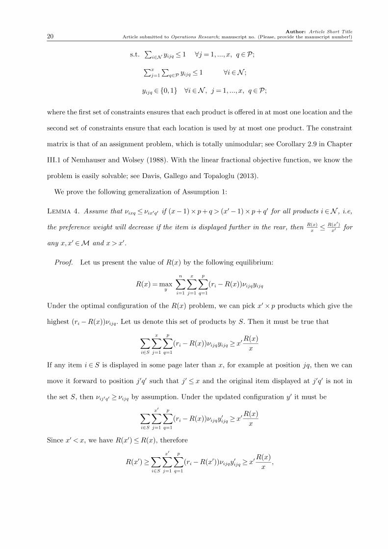
s.t.∑
i∈N yijq ≤ 1 ∀j = 1, ..., x, q ∈P;∑x
j=1
∑q∈P yijq ≤ 1 ∀i∈N ;
yijq ∈ {0,1} ∀i∈N , j = 1, ..., x, q ∈P;
where the first set of constraints ensures that each product is offered in at most one location and the
second set of constraints ensure that each location is used by at most one product. The constraint
matrix is that of an assignment problem, which is totally unimodular; see Corollary 2.9 in Chapter
III.1 of Nemhauser and Wolsey (1988). With the linear fractional objective function, we know the
problem is easily solvable; see Davis, Gallego and Topaloglu (2013).
We prove the following generalization of Assumption 1:
Lemma 4. Assume that νixq ≤ νix′q′ if (x− 1)× p+ q > (x′− 1)× p+ q′ for all products i∈N , i.e,
the preference weight will decrease if the item is displayed further in the rear, then R(x)
x≤ R(x′)
x′ for
any x,x′ ∈M and x> x′.
Proof. Let us present the value of R(x) by the following equilibrium:
R(x) = maxy
n∑i=1
x∑j=1
p∑q=1
(ri−R(x))νijqyijq
Under the optimal configuration of the R(x) problem, we can pick x′× p products which give the
highest (ri−R(x))νijq. Let us denote this set of products by S. Then it must be true that
∑i∈S
x∑j=1
p∑q=1
(ri−R(x))νijqyijq ≥ x′R(x)
x
If any item i ∈ S is displayed in some page later than x, for example at position jq, then we can
move it forward to position j′q′ such that j′ ≤ x and the original item displayed at j′q′ is not in
the set S, then νij′q′ ≥ νijq by assumption. Under the updated configuration y′ it must be
∑i∈S
x′∑j=1
p∑q=1
(ri−R(x))νijqy′ijq ≥ x′
R(x)
x
Since x′ <x, we have R(x′)≤R(x), therefore
R(x′)≥∑i∈S
x′∑j=1
p∑q=1
(ri−R(x′))νijqy′ijq ≥ x′
R(x)
x,

Author: Article Short TitleArticle submitted to Operations Research; manuscript no. (Please, provide the manuscript number!) 21
which implies that
R(x′)
x′≥ R(x)
x.
�
With Lemma 4 and the increasing-failure-rate property, we can show that the 6π2
performance
bound still holds.
Theorem 7. Assume that νixq ≤ νix′q′ if (x− 1)× p+ q > (x′− 1)× p+ q′ for all products i ∈N .
Then then all bounds proved in Sections 6 continue to hold for the model with location preference.
8. Price Framing Problem
In reality the retailer cares about not only how to display the products, but also how to price
them to maximize the revenue. In this section we first consider the case where the products are
framed and the only issue is to find optimal prices. More precisely, we assume that an allocation
of products to pages is given, where yij ∈ {0,1}, and yij = 1 if and only if item i is displayed on
page j. Naturally∑
j yij = 1 and∑
i yij ≤ 1.
Similar to the model of Section 2, each consumer will only consider products on the first x pages
with probability λ(x), x= 1, . . . ,m. The decision variables are the price vector r= (r1, ..., rn)∈Rn+,
where ri denotes the price of item i. The consumer choice process is similar to the one in Section
2. Given the price ri for item i, the attractiveness of item i is vi = exp(ai− βri), where ai can be
considered as the price-independent quality of item i and β > 0 is the price sensitivity parameter.
By convention, the attractiveness of the no-purchase option is v0 = exp(0) ≡ 1. This formulation
assumes a linear utility structure commonly used in Economics, Marketing and Psychology (Berry,
Levinsohn and Pakes 1995; Fader and Hardie 1996; Shugan 1980).
Let Sx = {i : yix = 1} be the set of products displayed on page x. Then Sx = ∪xj=1Sj is the
consideration set of a consumer who views x pages. Assuming that the sets Sx, ∀x= 1, ...,m are
fixed, we can express the pricing problem as the following:
Rpricing = maxr R(r|S)≡∑m
x=1 λ(x)Rx(r|Sx) (7)

Author: Article Short Title22 Article submitted to Operations Research; manuscript no. (Please, provide the manuscript number!)
Where Rx(r|Sx) =∑
i∈Sx riP (i,Sx) is the expected profit from consumer x, and P (i,Sx) is the
probability that consumer x purchases item i:
P (i,Sx) =
exp(ai−βri)
1+∑
j∈Sx exp(aj−βrj), i∈ Sx,
0, otherwise.
We prove the following structural results:
Theorem 8. Assume that the configuration of products on m pages is given. At optimality, all
products on the same page have a same price. That is, there are page-dependent invariant parame-
ters θ= (θ1, ..., θm) such that ri = rk = θx if both products i and k are displayed on page x. Moreover
θ1 < θ2 < ... < θm.
This result extends the traditional assortment-pricing result under the MNL model. It is known
that the optimal prices under the MNL have a constant markup (see for example, Anderson, de
Palma and Thisse (1992), Hopp and Xu (2005) and Gallego and Stefanescu (2011)). We set the
costs to zero as we are looking into the revenue maximization problem, which is more relevant
when the costs are sunk. However, the structure still applies when the costs are nonzero as we are
maximizing the profit. Although the price under our model is no longer constant, we show that it
is page-dependent.
Therefore we can reduce the decision variables from n prices, one for each item, to m prices, one
for each page. The resulting problem in terms of θj, j = 1, . . . ,m is given by:
Rpricing = maxθ
R(θ|S)≡m∑x=1
λ(x)Rx(θ|Sx)≡m∑x=1
λ(x)
∑x
j=1 θj∑
i∈Sjexp (ai−βθj)
1 +∑x
j=1
∑i∈Sj
exp (ai−βθj)
The first order condition gives a system of equations:
∂R(θ|S)
∂θx=
m∑j=x
λ(j)P (Sx,Sj)(1−βθx +βRj(θ|Sj)) = 0 ∀x= 1 ...m
which is equivalent to
θx =1
β+
∑m
j=x λ(j)P (Sx,Sj)Rj(θ|Sj)∑m
j=x λ(j)P (Sx,Sj)=
1
β+
∑m
j=x λ(j)/V (Sj)Rj(θ|Sj)∑m
j=x λ(j)/V (Sj)

Author: Article Short TitleArticle submitted to Operations Research; manuscript no. (Please, provide the manuscript number!) 23
In other words, the price for page t’s products is a constant plus the weighted average of the
expected profit from the consumers who will view and therefore consider the products. And notice
that the ratio of weights is invariant for all consumer types.
In general, the expected profit R(θ|S) may not be jointly concave in the θ vector.
Example 1. Two products to be displayed on two pages. Therefore there are outcomes for the
number of pages viewed, one and two, with probability 56% and 44%, respectively. Product one
has quality a1 = 4 and item two has a2 = 2. Price sensitivity is equal to one. The graph below shows
how the expected profit changes with respect to the price. As we can see, the expected profit is
not jointly concave on the price vector.
Figure 1 Pricing Example
With the above optimal pricing structure, we now look into the problem of how we should order
the products linearly. A related question is whether all products should be displayed. We first

Author: Article Short Title24 Article submitted to Operations Research; manuscript no. (Please, provide the manuscript number!)
consider products that are differentiated only by their quality parameters ai, i= 1, ..., n. Without
loss of generality, we will assume that the products are ordered in decreasing quality, so that
a1 ≥ a2 ≥ ...≥ an.
Theorem 9. Assume that products differ in their quality parameters ai, i= 1, ..., n. At optimality,
each page is filled with products until all products are displayed. The products are displayed in order
of their indices, so that higher quality products are displayed earlier.
In essence, the combination of Theorems 8 and 9 tell us that higher-quality products should be
displayed first and with a lower price. This may be a bit unintuitive, and requires some explanation.
The prices are of the form ri = θx(i), where x(i) is the index of the page for product i, with
θ1 . . .≤ θm. Thus products seen by fewer people have a higher price, with the lowest price enjoyed
by products in page 1, which are seen by everybody. Interestingly, the price θ1, levied on the
highest quality products that appear in the first page is higher than the optimal price, that would
result if P (X ≤ 1) = 1; the price θm, levied on the lowest quality products that appear in the last
page is lower than the optimal price, that would result if P (X ≥m) = 1. In essence, consumers
are penalized for not being willing to see all products and are compensated for being willing to
see more products. Another way to understanding the result is that lower-quality products are
charged higher prices and serve to steer consumers to the higher-quality products, while earning
large prices should the consumer decide to purchase them. This result is in sharp contrast with the
results for pricing in an oligopoly market, where several firms are deciding prices.
Corollary 5. Under optimal pricing and display configuration, the expected profit Rx(r|Sx) for
a consumer who views x pages is increasing and concave with respect to x.
This result is intuitive as the objective function is increasing in the number of products and
consumers who look at more pages also look at more products.
The optimal analytical structure can also be extended to the profit maximization problem.
Interestingly, products now should be ordered by their net value, defined as the quality minus price
sensitivity times price, which is first introduced by Gallego, Li and Beltran (2016).

Author: Article Short TitleArticle submitted to Operations Research; manuscript no. (Please, provide the manuscript number!) 25
Corollary 6. For the profit maximization problem, at optimality, products are displayed in
decreasing order of their net values vi ≡ αi − βci, and they are priced with page-level constant
markups, i.e, ri− ci = θx(i).
This can be easily seen by replacing αi with the net value αi−βci.
9. Computational Experiments
In this section, we first numerically test the performance of the following framing algorithms:
• The NESTED (NEST) algorithm introduced in Section 6.
• The enhanced version NESTED+ (NEST+) introduced in Section 6.3, which is designed to
improve practical performance.
• A heuristic, SORT1, which sorts and displays products in increasing order of price.
• A heuristic, SORT2, which sorts and displays products in decreasing order of attractiveness.
Then we compare the performance of NEST+ with Price Framing algorithm( P+F ) and see how
much improvement can be achieved if we are able to jointly optimize over frame and prices.
9.1. Experimental Setup
We proceed by describing the instances being tested in our experiments. In all of our test problems,
we assume that customer choices are governed by the Multinomial Logit model. The MNL associates
the attractiveness {vi : i∈N} with products. If the set of products S(x) is displayed at the first x
pages, then conditional on consumer type x’s arrival, he will buy product i∈ S(x) with probability
vi1 +
∑i′∈S(x) vi′
.
By convention, vi = eai−βri , where ai is the product quality. In the tests, we independently draw
every ri from a uniform distribution over [70,80]. We set β = 1.02 and ai = ri + εi, where εi ∈
[−0.3,0.3] is a noise added to the quality of product i.
For all test cases of the framing algorithms, we use n= 300 and m= 20 . We test three different
distributions of X: geometric, uniform and Poisson. We also differentiate the simulation scenarios

Author: Article Short Title26 Article submitted to Operations Research; manuscript no. (Please, provide the manuscript number!)
by the expectation of X: Small (E(X) = 2), Median (E(X) = 4), and Large (E(X) = 8). We also
vary the number p of products in each page.
For the comparison between the NEST+ and the P+F algorithms, we set the test cases as n= 20
and m= 2; P (X = 1) = P (X = 2) = 0.5. Number of products p in each page varies. We simulate
a’s and r’s values as previously stated, and input them into the NEST+ algorithm. We compare
the expected revenue with the one returned by the P+F algorithm, which optimally frames the
products in decreasing order of a and can jointly optimize the r.
For each test case, we simulate 1,000 replicates and report the average gaps between the heuristics
and the upper bound, the maximum gaps found in all replicates, and the estimated chances that
the relative gaps falls within 0.01% and 0.2%.
9.2. Experimental Result
9.2.1. Results of Framing Algorithms Refer to Tables 1 to 9. In all scenarios and according
to our metrics, SORT2 out performs SORT1, and expectedly, NST+ outperforms NST . NST+
dominates both SORT1 and SORT2 heuristics, with average and maximum optimality gap of
just 0.25% and 0.84% in the worst case, compared to 5.8% and 7.44% for SORT2, respectively.
The optimality gaps SORT1 and SORT2 are relatively uniform across different scenarios, whereas
the optimality gaps for NST and NST+ tend to be larger for the geometric and exponential
distributions, which we have shown to be worst-case distributions for these algorithms.
Table 1 Performance of NESTED when E[X] = 2 and X follows a geometric distribution.
Avg gap Max gap P (gap≤ 0.01%) P (gap≤ 0.2%)
p NST NST+ SORT1 SORT2 NST NST+ SORT1 SORT2 NST+ NST+
1 11.94% 0.24% 17.68% 1.82% 12.63% 0.72% 30.13% 3.93% 0.022 0.448
3 5.67% 0.02% 14.31% 4.10% 6.06% 0.27% 21.91% 5.49% 0.666 0.996
9 9.56% 0.00% 11.85% 5.69% 10.01% 0.05% 15.84% 6.87% 0.925 1
15 6.22% 0.00% 10.85% 5.79% 6.52% 0.02% 12.51% 7.13% 0.986 1

Author: Article Short TitleArticle submitted to Operations Research; manuscript no. (Please, provide the manuscript number!) 27
Table 2 Performance of NESTED when E[X] = 4 and X follows a geometric distribution.
Avg gap Max gap P (gap≤ 0.01%) P (gap≤ 0.2%)
p NST NST+ SORT1 SORT2 NST NST+ SORT1 SORT2 NST+ NST+
1 9.95% 0.17% 15.45% 3.35% 10.61% 0.68% 24.58% 4.83% 0.011 0.713
3 7.29% 0.01% 12.80% 5.04% 7.86% 0.20% 17.91% 6.53% 0.621 0.999
9 5.76% 0.00% 10.67% 5.52% 6.11% 0.04% 12.46% 6.55% 0.943 1
15 10.49% 0.00% 9.53% 5.22% 11.07% 0.02% 10.65% 6.30% 0.983 1
Table 3 Performance of NESTED when E[X] = 8 and X follows a geometric distribution.
Avg gap Max gap P (gap≤ 0.01%) P (gap≤ 0.2%)
p NST NST+ SORT1 SORT2 NST NST+ SORT1 SORT2 NST+ NST+
1 10.58% 0.08% 13.76% 4.53% 11.01% 0.30% 19.94% 5.96% 0.013 0.982
3 8.55% 0.01% 11.64% 5.42% 9.01% 0.12% 14.08% 6.40% 0.707 1
9 8.87% 0.00% 9.30% 4.99% 9.37% 0.02% 10.62% 5.86% 0.986 1
15 5.16% 0.00% 7.66% 4.36% 5.66% 0.01% 8.51% 5.08% 0.998 1
Table 4 Performance of NESTED when E[X] = 2 and X follows a uniform distribution.
Avg gap Max gap P (gap≤ 0.01%) P (gap≤ 0.2%)
p NST NST+ SORT1 SORT2 NST NST+ SORT1 SORT2 NST+ NST+
1 0.24% 0.24% 17.44% 1.70% 0.83% 0.83% 32.26% 3.93% 0.051 0.425
3 4.92% 0.01% 14.20% 4.33% 5.21% 0.19% 23.00% 5.70% 0.656 1
9 11.65% 0.00% 11.72% 5.86% 12.04% 0.06% 14.32% 7.11% 0.89 1
15 7.70% 0.00% 10.70% 5.84% 8.08% 0.04% 12.23% 7.29% 0.96 1
9.2.2. Results of NEST+ Vs. P+F Refer to Tables 10. Obviously, in all scenarios, P+F out
performs NEST+. When 6 products are to be assigned to two pages, the two algorithm’s average
performance gap can be as high as 44.9%. The gap decreases as the number of products p held in
each page increases. This is because the Price Framing algorithms tends to steer all customers to

Author: Article Short Title28 Article submitted to Operations Research; manuscript no. (Please, provide the manuscript number!)
Table 5 Performance of NESTED when E[X] = 4 and X follows a uniform distribution.
Avg gap Max gap P (gap≤ 0.01%) P (gap≤ 0.2%)
p NST NST+ SORT1 SORT2 NST NST+ SORT1 SORT2 NST+ NST+
1 3.63% 0.10% 15.21% 3.47% 4.02% 0.44% 24.72% 5.00% 0.016 0.935
3 7.91% 0.01% 12.60% 5.44% 8.26% 0.14% 16.40% 6.61% 0.706 1
9 6.91% 0.00% 10.51% 5.63% 7.29% 0.03% 12.08% 6.82% 0.973 1
15 4.27% 0.00% 9.44% 5.18% 4.66% 0.01% 10.52% 6.21% 0.999 1
Table 6 Performance of NESTED when E[X] = 8 and X follows a uniform distribution.
Avg gap Max gap P (gap≤ 0.01%) P (gap≤ 0.2%)
p NST NST+ SORT1 SORT2 NST NST+ SORT1 SORT2 NST+ NST+
1 6.18% 0.05% 13.47% 4.89% 8.05% 0.25% 18.49% 6.27% 0.025 0.998
3 6.73% 0.01% 11.27% 5.68% 7.06% 0.04% 13.40% 6.97% 0.797 1
9 5.81% 0.00% 9.02% 4.92% 6.25% 0.02% 9.90% 5.71% 0.995 1
15 4.01% 0.00% 7.28% 4.11% 6.16% 0.01% 7.91% 4.89% 1 1
Table 7 Performance of NESTED when E[X] = 2 and X follows a Poisson distribution.
Avg gap Max gap P (gap≤ 0.01%) P (gap≤ 0.2%)
p NST NST+ SORT1 SORT2 NST NST+ SORT1 SORT2 NST+ NST+
1 9.62% 0.17% 17.30% 1.72% 10.11% 0.54% 30.90% 4.28% 0.035 0.638
3 4.82% 0.01% 14.21% 4.29% 5.10% 0.22% 22.14% 5.66% 0.654 0.999
9 11.12% 0.00% 11.73% 5.82% 11.53% 0.05% 14.56% 7.01% 0.879 1
15 7.33% 0.00% 10.75% 5.84% 7.72% 0.05% 12.41% 7.00% 0.972 1
the first page, therefore the revenue contribution of the second page will be less prominent as the
p increases.

Author: Article Short TitleArticle submitted to Operations Research; manuscript no. (Please, provide the manuscript number!) 29
Table 8 Performance of NESTED when E[X] = 4 and X follows a Poisson distribution.
Avg gap Max gap P (gap≤ 0.01%) P (gap≤ 0.2%)
p NST NST+ SORT1 SORT2 NST NST+ SORT1 SORT2 NST+ NST+
1 6.30% 0.05% 15.22% 3.40% 6.61% 0.22% 24.14% 5.46% 0.041 0.998
3 6.96% 0.00% 12.60% 5.57% 7.25% 0.06% 16.67% 6.97% 0.841 1
9 7.01% 0.00% 10.41% 5.74% 7.44% 0.04% 11.59% 6.97% 0.974 1
15 4.38% 0.00% 9.39% 5.22% 4.67% 0.01% 10.17% 6.27% 0.999 1
Table 9 Performance of NESTED when E[X] = 8 and X follows a Poisson distribution.
Avg gap Max gap P (gap≤ 0.01%) P (gap≤ 0.2%)
p NST NST+ SORT1 SORT2 NST NST+ SORT1 SORT2 NST+ NST+
1 5.53% 0.01% 13.33% 5.04% 5.78% 0.07% 20.20% 6.44% 0.797 1
3 3.87% 0.00% 11.08% 5.99% 4.09% 0.03% 13.28% 7.26% 0.987 1
9 2.29% 0.00% 8.92% 4.95% 2.51% 0.00% 9.57% 6.16% 1 1
15 1.94% 0.00% 7.25% 4.05% 2.23% 0.00% 8.17% 4.94% 1 1
Table 10 Performance improvement of P+F over NEST+
p Avg gap Max gap
3 44.9% 48.3%
6 30.2% 33.1%
9 23.3% 26.2%
10. Conclusion and Future Work
In this work, we propose one of the first models of “framing effects” for pricing and assortment
optimization. We introduce a model in which a set of products must be organized sequentially
into a set of virtual pages and priced appropriately. Each consumers will only consider a random
number of pages, and will select a item, if any, from these pages following a general choice model.
We show that this product-framing problem is NP-hard. We derive algorithms with guaranteed
Author: Article Short Title30 Article submitted to Operations Research; manuscript no. (Please, provide the manuscript number!)
relative performance. Our algorithms are fast, easy to implement, and dominate the best known
performance bounds. We also show new structural results for pricing under framing effects. In the
future, it is worthwhile to endogenize the pages’ viewing probability λ(·)’s. So far we assume that
they are independent of the display. In the context of dynamic search, it is more practical to assume
the λ(·)’s and the framing are correlated.
11. Appendix
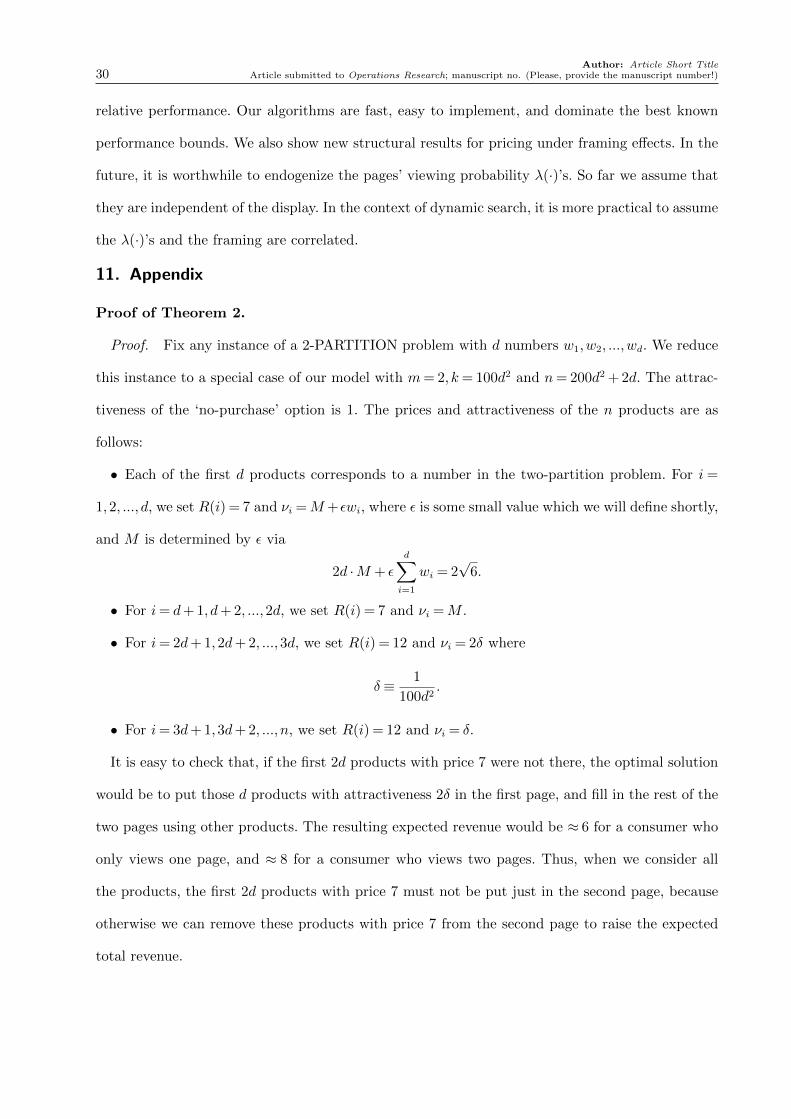
Proof of Theorem 2.
Proof. Fix any instance of a 2-PARTITION problem with d numbers w1,w2, ...,wd. We reduce
this instance to a special case of our model with m= 2, k= 100d2 and n= 200d2 + 2d. The attrac-
tiveness of the ‘no-purchase’ option is 1. The prices and attractiveness of the n products are as
follows:
• Each of the first d products corresponds to a number in the two-partition problem. For i=
1,2, ..., d, we set R(i) = 7 and νi =M+εwi, where ε is some small value which we will define shortly,
and M is determined by ε via
2d ·M + εd∑i=1
wi = 2√
6.
• For i= d+ 1, d+ 2, ...,2d, we set R(i) = 7 and νi =M .
• For i= 2d+ 1,2d+ 2, ...,3d, we set R(i) = 12 and νi = 2δ where
δ≡ 1
100d2.
• For i= 3d+ 1,3d+ 2, ..., n, we set R(i) = 12 and νi = δ.
It is easy to check that, if the first 2d products with price 7 were not there, the optimal solution
would be to put those d products with attractiveness 2δ in the first page, and fill in the rest of the
two pages using other products. The resulting expected revenue would be ≈ 6 for a consumer who
only views one page, and ≈ 8 for a consumer who views two pages. Thus, when we consider all
the products, the first 2d products with price 7 must not be put just in the second page, because
otherwise we can remove these products with price 7 from the second page to raise the expected
total revenue.
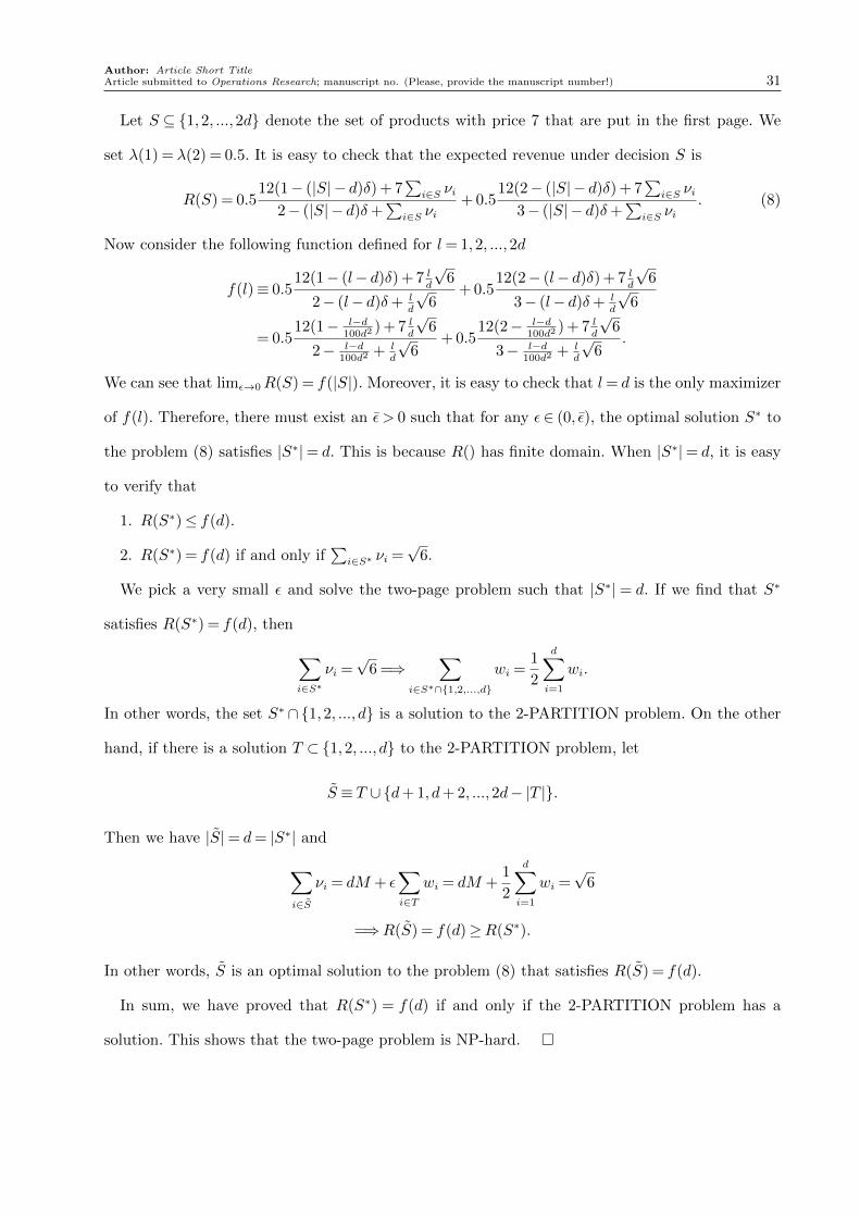
Author: Article Short TitleArticle submitted to Operations Research; manuscript no. (Please, provide the manuscript number!) 31
Let S ⊆ {1,2, ...,2d} denote the set of products with price 7 that are put in the first page. We
set λ(1) = λ(2) = 0.5. It is easy to check that the expected revenue under decision S is
R(S) = 0.512(1− (|S| − d)δ) + 7
∑i∈S νi
2− (|S| − d)δ+∑
i∈S νi+ 0.5
12(2− (|S| − d)δ) + 7∑
i∈S νi
3− (|S| − d)δ+∑
i∈S νi. (8)
Now consider the following function defined for l= 1,2, ...,2d
f(l)≡ 0.512(1− (l− d)δ) + 7 l
d
√6
2− (l− d)δ+ ld
√6
+ 0.512(2− (l− d)δ) + 7 l
d
√6
3− (l− d)δ+ ld
√6
= 0.512(1− l−d
100d2) + 7 l
d
√6
2− l−d100d2
+ ld
√6
+ 0.512(2− l−d
100d2) + 7 l
d
√6
3− l−d100d2
+ ld
√6
.
We can see that limε→0R(S) = f(|S|). Moreover, it is easy to check that l= d is the only maximizer
of f(l). Therefore, there must exist an ε > 0 such that for any ε∈ (0, ε), the optimal solution S∗ to
the problem (8) satisfies |S∗|= d. This is because R() has finite domain. When |S∗|= d, it is easy
to verify that
1. R(S∗)≤ f(d).
2. R(S∗) = f(d) if and only if∑
i∈S∗ νi =√
6.
We pick a very small ε and solve the two-page problem such that |S∗| = d. If we find that S∗
satisfies R(S∗) = f(d), then
∑i∈S∗
νi =√
6 =⇒∑
i∈S∗∩{1,2,...,d}
wi =1
2
d∑i=1
wi.
In other words, the set S∗ ∩{1,2, ..., d} is a solution to the 2-PARTITION problem. On the other
hand, if there is a solution T ⊂ {1,2, ..., d} to the 2-PARTITION problem, let
S ≡ T ∪{d+ 1, d+ 2, ...,2d− |T |}.
Then we have |S|= d= |S∗| and
∑i∈S
νi = dM + ε∑i∈T
wi = dM +1
2
d∑i=1
wi =√
6
=⇒R(S) = f(d)≥R(S∗).
In other words, S is an optimal solution to the problem (8) that satisfies R(S) = f(d).
In sum, we have proved that R(S∗) = f(d) if and only if the 2-PARTITION problem has a
solution. This shows that the two-page problem is NP-hard. �

Author: Article Short Title32 Article submitted to Operations Research; manuscript no. (Please, provide the manuscript number!)
Proof of Theorem 6.
Proof. It is clear that under our algorithm
R(x)−R(y)
x− y≥ R(m)−R(y)
m− y.
Consequently
V NEST+(y) ≥ R(y)
yEmin(X,y) +
R(m)−R(y)
m− yE[(X − y)+]
=R(y)
yE[X]−
(R(y)
y− R(m)−R(y)
m− y
)E[(X − y)+].
Setting y= µ, and using the bound E[(X −µ)+]≤ µe−1 we obtain,
V NEST+(µ)
E[R(X)]≥ aµ− (a− b)µe−1
aµ
≥ 1− (1− b
a)e−1
=e− 1
e+
1
e
b
a.
�
Proof of Theorem 8.
Proof. Given the sets Sx, ∀x= 1, ...,m fixed, we maximize solely over prices. That is, we want
to compute
maxrR(r|S) =
m∑x=1
λ(x)Rx(r|Sx) =m∑x=1
λ(x)∑i∈Sx
riP (i,Sx),
where Rx(r|Sx) is the expected profit from consumer who has consideration set Sx and P (i,Sx) =
exp(ai−βri)1+
∑k∈Sx exp(ak−βrk)
is the probability of choosing item i if i is in consumer x’s consideration set.
Taking partial derivative of P (i,Sx) with respect to product i’s and k’s prices ri and rk respectively,
we have the following formulas:
∂P (i,Sx)∂ri
= βP (i,Sx)(P (i,Sx)− 1), and
∂P (i,Sx)∂rk
= βP (i,Sx)P (k,Sx).
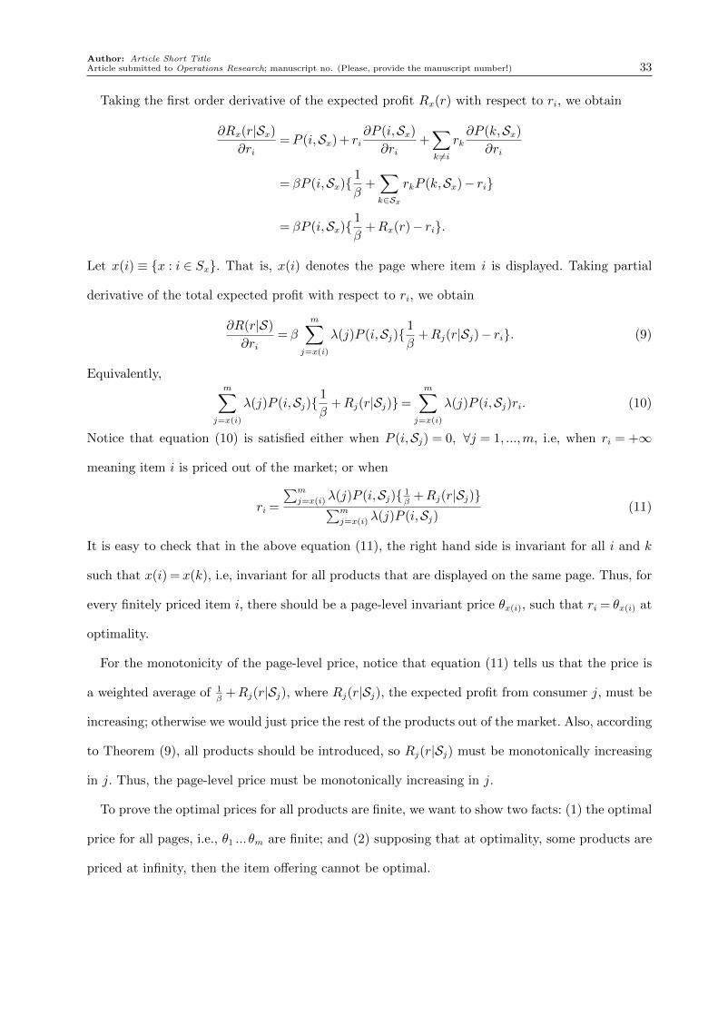
Author: Article Short TitleArticle submitted to Operations Research; manuscript no. (Please, provide the manuscript number!) 33
Taking the first order derivative of the expected profit Rx(r) with respect to ri, we obtain
∂Rx(r|Sx)∂ri
= P (i,Sx) + ri∂P (i,Sx)
∂ri+∑k 6=i
rk∂P (k,Sx)
∂ri
= βP (i,Sx){1
β+∑k∈Sx
rkP (k,Sx)− ri}
= βP (i,Sx){1
β+Rx(r)− ri}.
Let x(i) ≡ {x : i ∈ Sx}. That is, x(i) denotes the page where item i is displayed. Taking partial
derivative of the total expected profit with respect to ri, we obtain
∂R(r|S)
∂ri= β
m∑j=x(i)
λ(j)P (i,Sj){1
β+Rj(r|Sj)− ri}. (9)
Equivalently,m∑
j=x(i)
λ(j)P (i,Sj){1
β+Rj(r|Sj)}=
m∑j=x(i)
λ(j)P (i,Sj)ri. (10)
Notice that equation (10) is satisfied either when P (i,Sj) = 0, ∀j = 1, ...,m, i.e, when ri = +∞
meaning item i is priced out of the market; or when
ri =
∑m
j=x(i) λ(j)P (i,Sj){ 1β
+Rj(r|Sj)}∑m
j=x(i) λ(j)P (i,Sj)(11)
It is easy to check that in the above equation (11), the right hand side is invariant for all i and k
such that x(i) = x(k), i.e, invariant for all products that are displayed on the same page. Thus, for
every finitely priced item i, there should be a page-level invariant price θx(i), such that ri = θx(i) at
optimality.
For the monotonicity of the page-level price, notice that equation (11) tells us that the price is
a weighted average of 1β
+Rj(r|Sj), where Rj(r|Sj), the expected profit from consumer j, must be
increasing; otherwise we would just price the rest of the products out of the market. Also, according
to Theorem (9), all products should be introduced, so Rj(r|Sj) must be monotonically increasing
in j. Thus, the page-level price must be monotonically increasing in j.
To prove the optimal prices for all products are finite, we want to show two facts: (1) the optimal
price for all pages, i.e., θ1 ... θm are finite; and (2) supposing that at optimality, some products are
priced at infinity, then the item offering cannot be optimal.

Author: Article Short Title34 Article submitted to Operations Research; manuscript no. (Please, provide the manuscript number!)
The first fact is equivalent to having θm < +∞, since we know that the page-level price θx
is monotonically increasing in x. The first-order condition given by page m implies θm = 1β
+
Rm(θ|Sm), which proves the finiteness of θm.
Consider the second fact that we need to prove. Notice that having some prices equal to infinity
is equivalent to pricing the corresponding products out of the market, or not displaying them at all.
Equivalently, there is some page x displaying fewer than p products. Therefore we can introduce
one more item without increasing the total attractiveness of page x. This can be achieved by
increasing products’ prices on page x. In this situation, the expected profit from consumer segment
x′ = 1...x− 1 will not be affected, and the expected profit from segment x and larger will strictly
increase. That is, Rx′(r|Sx′), x′ = x...m, will become larger. Thus, the total expected profit will
strictly increase when we fill all pages with finitely priced products. �
Proof of Theorem 9.
Proof. Suppose that the page configuration Sx is fixed for all x = 1, ...,m. Given the quality
vector a= (a1, ..., an), we want to optimize with respect to prices. That is, we want to solve
R(a) = maxr R(r|S)≡∑m
x=1 λ(x)Rx(r|Sx). (12)
Now, suppose we can change the vector a. We wish to determine how the optimal profit R(a) will
change. Let us take the partial derivative of R(a) with respect to ai.
∂R(a)
∂ai=
m∑j=x(i)
λ(j)∂Rj(r(a)|Sj)
∂ai
=m∑
j=x(i)
λ(j){ri(a)−Rj(r(a)|Sj)}P (i,Sj), (13)
where r(a) is the optimal price vector under quality vector a, which must satisfy the first-order
condition given by (11), i.e,∑m
j=x(i) λ(j)P (i,Sj)ri(a) =∑m
j=x(i) λ(j)P (i,Sj){ 1β
+Rj(r(a)|Sj)}. Plug
this relationship into (13), we obtain
∂R(a)
∂ai=
1
β
m∑j=x(i)
λ(j)P (i,Sj). (14)

Author: Article Short TitleArticle submitted to Operations Research; manuscript no. (Please, provide the manuscript number!) 35
From the above relationship, we can draw several conclusions. First, the optimal profit R(a) is
increasing in ai for all i = 1, ..., n. Second, suppose there are two item i and k with the same
quality ai = ak, but x(i)<x(k), in other words, i is displayed before k so it can be viewed by more
consumer. Equation (14) tells us ∂R(a)
∂ai> ∂R(a)
∂ak, so if we can increase ai or ak, it is always better to
increase ai. This indicates that products should be displayed in decreasing order of their quality.
To prove that all products should be displayed, notice that eliminating item i is equivalent to
letting its quality ai go to negative infinity. However, since ∂R(a)
∂ai> 0 and it is always better to
put products with higher quality ahead of products with lower quality, we can conclude that at
optimality, all products should be displayed; and they are displayed in the order of their indices.
Each page is filled up with products until its capacity is saturated. �
References
Agarwal, Ashish, Kartik Hosanagar, Michael D. Smith. 2011. Location, location, location: An analysis of
profitability of position in online advertising markets. Journal of Marketing Research 48(6) 1057–1073.
doi:10.1509/jmr.08.0468. URL http://dx.doi.org/10.1509/jmr.08.0468.
Amos Tversky, Daniel Kahneman. 1986. Rational choice and the framing of decisions. The Journal of
Business 59(4) S251–S278. URL http://www.jstor.org/stable/2352759.
Anderson, Simon P, Andre De Palma, Jacques Francois Thisse. 1992. Discrete choice theory of product
differentiation. MIT press.
Animesh, Animesh, Siva Viswanathan, Ritu Agarwal. 2011. Competing “creatively” in sponsored search
markets: The effect of rank, differentiation strategy, and competition on performance. Information
Systems Research 22(1) 153–169. doi:10.1287/isre.1090.0254. URL http://pubsonline.informs.
org/doi/abs/10.1287/isre.1090.0254.
Aouad, Ali, Danny Segev. 2016. Display optimization for vertically differentiated locations under multinomial
logit choice preferences. Tech. rep., Working Paper.
Arbatskaya, Maria. 2007. Ordered search. The RAND Journal of Economics 38(1) 119–126. URL http:
//www.jstor.org/stable/25046295.
Author: Article Short Title36 Article submitted to Operations Research; manuscript no. (Please, provide the manuscript number!)
Baye, Michael R., J. Rupert J. Gatti, Paul Kattuman, John Morgan. 2009. Clicks, discontinuities, and firm
demand online. Journal of Economics & Management Strategy 18(4) 935–975. doi:10.1111/j.1530-9134.
2009.00234.x. URL http://dx.doi.org/10.1111/j.1530-9134.2009.00234.x.
Berry, Steven, James Levinsohn, Ariel Pakes. 1995. Automobile Prices in Market Equilibrium. Econometrica
63(4) 841–90. URL https://ideas.repec.org/a/ecm/emetrp/v63y1995i4p841-90.html.
Bront, J.J.M., I. Mendez-Diaz, G. Vulcano. 2009. A column generation algorithm for choice-based network
revenue management. Operations Research 57(3) 769–784.
Brynjolfsson, Erik, Astrid A. Dick, Michael D. Smith. 2010. A nearly perfect market? : differentiation vs.
price in consumer choice.
Cachon, Gerard P., Christian Terwiesch, Yi Xu. 2005. Retail assortment planning in the presence of consumer
search. Manufacturing & Service Operations Management 7(4) 330–346. doi:10.1287/msom.1050.0088.
URL http://dx.doi.org/10.1287/msom.1050.0088.
Chandon, Pierre, J. Wesley Hutchinson, Eric T. Bradlow, Scott H. Young. 2009. Does in-store marketing
work? effects of the number and position of shelf facings on brand attention and evaluation at the point
of purchase. Journal of Marketing 73(6) 1–17. doi:10.1509/jmkg.73.6.1. URL http://dx.doi.org/
10.1509/jmkg.73.6.1.
Chiang, Jeongwen, Siddhartha Chib, Chakravarthi Narasimhan. 1998. Markov chain monte carlo and models
of consideration set and parameter heterogeneity. Journal of Econometrics 89(1–2) 223 – 248. doi:
http://dx.doi.org/10.1016/S0304-4076(98)00062-1. URL http://www.sciencedirect.com/science/
article/pii/S0304407698000621.
Davis, James, Guillermo Gallego, Huseyin Topaloglu. 2013. Assortment planning under the multinomial
logit model with totally unimodular constraint structures. Tech. rep., Working paper.
Davis, James M., Guillermo Gallego, Huseyin Topaloglu. 2014. Assortment optimization under variants
of the nested logit model. Operations Research 62(2) 250–273. doi:10.1287/opre.2014.1256. URL
http://dx.doi.org/10.1287/opre.2014.1256.
Davis, James M., Huseyin Topaloglu, David P. Williamson. 2015. Assortment optimization over time.
Operations Research Letters 43(6) 608 – 611. doi:http://dx.doi.org/10.1016/j.orl.2015.08.007. URL
http://www.sciencedirect.com/science/article/pii/S0167637715001108.

Author: Article Short TitleArticle submitted to Operations Research; manuscript no. (Please, provide the manuscript number!) 37
Desir, Antoine, Vineet Goyal. 2013. Near-optimal algorithms for capacity constrained assortment optimiza-
tion. Tech. rep., Working paper.
Feldman, J., H. Topaloglu. 2015. Assortment optimization under the multinomial logit model with nested
consideration sets. Tech. rep., Working Paper.
Feng, Juan, Hemant K. Bhargava, David M. Pennock. 2007. Implementing sponsored search in web search
engines: Computational evaluation of alternative mechanisms. INFORMS Journal on Computing 19(1)
137–148. doi:10.1287/ijoc.1050.0135. URL http://dx.doi.org/10.1287/ijoc.1050.0135.
Gallego, Guillermo, Anran Li, Jose Beltran. 2016. Product line design and pricing under logit model. Tech.
rep., Columbia University.
Gallego, Guillermo, Catalina Stefanescu. 2009. Upgrades, upsells and pricing in revenue management. Tech.
rep., Working Paper.
Gallego, Guillermo, Huseyin Topaloglu. 2014. Constrained assortment optimization for the nested logit
model. Management Science 60(10) 2583–2601. doi:10.1287/mnsc.2014.1931. URL http://dx.doi.
org/10.1287/mnsc.2014.1931.
Gallego, Guillermo, Ruxian Wang. 2014. Multiproduct price optimization and competition under the nested
logit model with product-differentiated price sensitivities. Operations Research 62(2) 450–461. doi:
10.1287/opre.2013.1249. URL http://dx.doi.org/10.1287/opre.2013.1249.
Ghose, Anindya, Sha Yang. 2009. An empirical analysis of search engine advertising: Sponsored search
in electronic markets. Management Science 55(10) 1605–1622. doi:10.1287/mnsc.1090.1054. URL
http://dx.doi.org/10.1287/mnsc.1090.1054.
Hauser, John R. 1978. Testing the accuracy, usefulness, and significance of probabilistic choice models: An
information-theoretic approach. Operations Research 26(3) 406–421. URL http://www.jstor.org/
stable/169752.
Hauser, John R., Steven P. Gaskin. 1984. Application of the defender consumer model. Marketing Science
3(4) 327–351. doi:10.1287/mksc.3.4.327. URL http://dx.doi.org/10.1287/mksc.3.4.327.

Author: Article Short Title38 Article submitted to Operations Research; manuscript no. (Please, provide the manuscript number!)
Hopp, Wallace J., Xiaowei Xu. 2005. Product line selection and pricing with modularity in design. Man-
ufacturing & Service Operations Management 7(3) 172–187. doi:10.1287/msom.1050.0077. URL
http://dx.doi.org/10.1287/msom.1050.0077.
Howard, J.A., J.N. Sheth. 1969. The theory of buyer behavior . Wiley marketing series, Wiley. URL https:
//books.google.com.hk/books?id=HOmRAAAAIAAJ.
Johnson, Eric J., Wendy W. Moe, Peter S. Fader, Steven Bellman, Gerald L. Lohse. 2004. On the depth and
dynamics of online search behavior. Manage. Sci. 50(3) 299–308. doi:10.1287/mnsc.1040.0194. URL
http://dx.doi.org/10.1287/mnsc.1040.0194.
Li, Hongmin, Woonghee Tim Huh. 2011. Pricing multiple products with the multinomial logit and nested
logit models: Concavity and implications. Manufacturing & Service Operations Management 13(4)
549–563. doi:10.1287/msom.1110.0344. URL http://pubsonline.informs.org/doi/abs/10.1287/
msom.1110.0344.
Manrai, Ajay K, Rick L Andrews. 1998. Two-stage discrete choice models for scanner panel data: An assess-
ment of process and assumptions. European Journal of Operational Research 111(2) 193 – 215. doi:
http://dx.doi.org/10.1016/S0377-2217(98)00145-3. URL http://www.sciencedirect.com/science/
article/pii/S0377221798001453.
Mittal, Shashi, Andreas S. Schulz. 2013. A general framework for designing approximation schemes for
combinatorial optimization problems with many objectives combined into one. Operations Research
61(2) 386–397. doi:10.1287/opre.1120.1093. URL http://dx.doi.org/10.1287/opre.1120.1093.
Nemhauser, George L., Laurence A. Wolsey. 1988. Integer and Combinatorial Optimization. Wiley-
Interscience, New York, NY, USA.
Peter S. Fader, Bruce G. S. Hardie. 1996. Modeling consumer choice among skus. Journal of Marketing
Research 33(4) 442–452. URL http://www.jstor.org/stable/3152215.
Sahin, Ozge, Ruxian Wang. 2014. The impact of consumer search cost on assortment planning and pricing.
Tech. rep., Working Paper.
Shugan, Steven M. 1980. The cost of thinking. Journal of Consumer Research 7(2) 99–111. URL http:
//www.jstor.org/stable/2489077.

Author: Article Short TitleArticle submitted to Operations Research; manuscript no. (Please, provide the manuscript number!) 39
Silk, Alvin J, Glen L Urban. 1978. Pre-test-market evaluation of new packaged goods: A model and mea-
surement methodology. Journal of marketing Research 171–191.
Song, Jing-sheng, Zhengliang Xue. 2009. Demand management and inventory control for substitutable
products. Tech. rep., Working Paper.
Talluri, K., G. Van Ryzin. 2004. Revenue management under a general discrete choice model of consumer
behavior. Management Science 50(1) 15–33.
Van Ryzin, G., S. Mahajan. 1999. On the relationship between inventory costs and variety benefits in retail
assortments. Management Science 45(11) 1496–1509.
Ward Hanson, Kipp Martin. 1996. Optimizing multinomial logit profit functions. Management Science 42(7)
992–1003. URL http://www.jstor.org/stable/2634363.