arX

iv:1

404.

4772

v2 [

mat

h.O

C]

16

Jun

2014

Approximating Pareto Curves usingSemidefinite Relaxations

Victor Magron1,2 Didier Henrion1,2,3 Jean-Bernard Lasserre1,2

June 17, 2014

Abstract

We consider the problem of constructing an approximation of the Pareto curveassociated with the multiobjective optimization problem minx∈S{(f1(x), f2(x))},where f1 and f2 are two conflicting polynomial criteria and S ⊂ Rn is a compactbasic semialgebraic set. We provide a systematic numerical scheme to approximatethe Pareto curve. We start by reducing the initial problem into a scalarized poly-nomial optimization problem (POP). Three scalarization methods lead to considerdifferent parametric POPs, namely (a) a weighted convex sum approximation, (b)a weighted Chebyshev approximation, and (c) a parametric sublevel set approxima-tion. For each case, we have to solve a semidefinite programming (SDP) hierarchyparametrized by the number of moments or equivalently the degree of a polynomialsums of squares approximation of the Pareto curve. When the degree of the poly-nomial approximation tends to infinity, we provide guarantees of convergence to thePareto curve in L2-norm for methods (a) and (b), and L1-norm for method (c).

Keywords Parametric Polynomial Optimization Problems, Semidefinite Programming,Multicriteria Optimization, Sums of Squares Relaxations, Pareto Curve, Inverse Problemfrom Generalized Moments

1 Introduction

Let P be the bicriteria polynomial optimization problem minx∈S{(f1(x), f2(x))}, whereS ⊂ R

n is the basic semialgebraic set:

S := {x ∈ Rn : g1(x) ≥ 0, . . . , gm(x) ≥ 0} , (1)

for some polynomials f1, f2, g1, . . . , gm ∈ R[x]. Here, we assume the following:

1CNRS; LAAS; 7 avenue du colonel Roche, F-31400 Toulouse; France.2Université de Toulouse; LAAS, F-31400 Toulouse, France.3Faculty of Electrical Engineering, Czech Technical University in Prague, Technická 2, CZ-16626

Prague, Czech Republic

1

Assumption 1.1. The image space R2 is partially ordered with the positive orthant R2

+.That is, given x ∈ R

2 and y ∈ R2, it holds x ≥ y whenever x − y ∈ R

2+.

For the multiobjective optimization problem P, one is usually interested in computing, orat least approximating, the following optimality set, defined e.g. in [6, Definition 11.5].

Definition 1.2. Let Assumption 1.1 be satisfied. A point x̄ ∈ S is called an Edgeworth-Pareto (EP) optimal point of Problem P, when there is no x ∈ S such that fj(x) ≤fj(x̄), j = 1, 2 and f(x) 6= f(x̄). A point x̄ ∈ S is called a weakly Edgeworth-Paretooptimal point of Problem P, when there is no x ∈ S such that fj(x) < fj(x̄), j = 1, 2.

In this paper, for conciseness, we will also use the following terminology:

Definition 1.3. The image set of weakly Edgeworth-Pareto optimal points is called thePareto curve.

Given a positive integer p and λ ∈ [0, 1] both fixed, a common workaround consists insolving the scalarized problem:

f p(λ) := minx∈S

{[(λf1(x))p + ((1 − λ)f2(x))p]1/p} , (2)

which includes the weighted sum approximation (p = 1)

P1λ : f 1(λ) := min

x∈S(λf1(x) + (1 − λ)f2(x)) , (3)

and the weighted Chebyshev approximation (p = ∞)

P∞

λ : f∞(λ) := minx∈S

max{λf1(x), (1 − λ)f2(x)} . (4)

Here, we assume that for almost all (a.a.) λ ∈ [0, 1], the solution x∗(λ) of the scalarizedproblem (3) (resp. (4)) is unique. Non-uniqueness may be tolerated on a Borel set B ⊂[0, 1], in which case one assumes image uniqueness of the solution. Then, by computinga solution x∗(λ), one can approximate the set {(f ∗

1 (λ), f ∗2 (λ)) : λ ∈ [0, 1]}, where

f ∗

j (λ) := fj(x∗(λ)), j = 1, 2.

Other approaches include using a numerical scheme such as the modified Polak method[11]: first, one considers a finite discretization (y

(k)1 ) of the interval [a1, b1], where

a1 := minx∈S

f1(x), b1 := f1(x) , (5)

with x being a solution of minx∈S f2(x). Then, for each k, one computes an optimal

solution xk of the constrained optimization problem y(k)2 := minx∈S{f2(x) : f1(x) = y

(k)1 }

and select the Pareto front from the finite collection {(y(k)1 , y

(k)2 )}. This method can

be improved with the iterative Eichfelder-Polak algorithm, see e.g. [3]. Assuming thesmoothness of the Pareto curve, one can use the Lagrange multiplier of the equalityconstraint to select the next point y

(k+1)1 . It allows to combine the adaptive control of

discretization points with the modified Polak method. In [2], Das and Dennis introduce

2

the Normal-boundary intersection method which can find a uniform spread of points onthe Pareto curve with more than two conflicting criteria and without assuming that thePareto curve is either connected or smooth. However, there is no guarantee that the NBImethod succeeds in general and even in case it works well, the spread of points is onlyuniform under certain additional assumptions. Interactive methods such as STEM [1] relyon a decision maker to select at each iteration the weight λ (most often in the case p = ∞)and to make a trade-off between criteria after solving the resulting scalar optimizationproblem.

So discretization methods suffer from two major drawbacks. (i) They only provide a finitesubset of the Pareto curve and (ii) for each discretization point one has to compute a globalminimizer of the resulting optimization problem (e.g. (3) or (4)). Notice that when f andS are both convex then point (ii) is not an issue.

In a recent work [4], Gorissen and den Hertog avoid discretization schemes for convexproblems with multiple linear criteria f1, f2, . . . , fk and a convex polytope S. They providean inner approximation of f(S) + R

k+ by combining robust optimization techniques with

semidefinite programming; for more details the reader is referred to [4].

Contribution. We provide a numerical scheme with two characteristic features: Itavoids a discretization scheme and approximates the Pareto curve in a relatively strongsense. More precisely, the idea is consider multiobjective optimization as a particularinstance of parametric polynomial optimization for which some strong approximation re-sults are available when the data are polynomials and semi-algebraic sets. In fact we willinvestigate this approach:

method (a) for the first formulation (3) when p = 1, this is a weighted convex sumapproximation;

method (b) for the second formuation (4) when p = ∞, this is a weighted Chebyshevapproximation;

method (c) for a third formulation inspired by [4], this is a parametric sublevel setapproximation.

When using some weighted combination of criteria (p = 1, method (a) or p = ∞, method(b)) we treat each function λ 7→ fj(λ), j = 1, 2, as the signed density of the signed Borelmeasure dµj := fj(λ)dλ with respect to the Lebesgue measure dλ on [0, 1]. Then theprocedure consists of two distinct steps:

1. In a first step, we solve a hierarchy of semidefinite programs (called SDP hierarchy)which permits to approximate any finite number s + 1 of moments mj := (mk

j ), k =0, . . . , s where :

mkj :=

∫ 1

0λkf ∗

j (λ)dλ , k = 0, . . . , s , j = 1, 2 .

More precisely, for any fixed integer s, step d of the SDP hierarchy provides anapproximation md

j of mj which converges to mj as d → ∞.

3

2. The second step consists of two density estimation problems: namely, for eachj = 1, 2, and given the moments mj of the measure f ∗

j dλ with unknown density f ∗j

on [0, 1], one computes a univariate polynomial hs,j ∈ Rs[λ] which solves the opti-mization problem minh∈Rs[λ]

∫ 10 (f ∗

j (λ)−h)2dλ if the moments mj are known exactly.The corresponding vector of coefficients hs

j ∈ Rs+1 is given by hs

j = Hs(λ)−1mj ,j = 1, 2, where Hs(λ) is the s-moment matrix of the Lebesgue measure dλ on [0, 1];therefore in the expression for hs

j we replace mj with its approximation.

Hence for both methods (a) and (b), we have L2-norm convergence guarantees.

Alternatively, in our method (c), one can estimate the Pareto curve by solving for eachλ ∈ [a1, b1] the following parametric POP:

Puλ : fu(λ) := min

x∈S{ f2(x) : f1(x) ≤ λ } , (6)

with a1 and b1 as in (5). Notice that by definition fu(λ) = f ∗2 (λ). Then, we derive an

SDP hierarchy parametrized by d, so that the optimal solution q2d ∈ R[λ]2d of the d-threlaxation underestimates f ∗

2 over [a1, b1]. In addition, q2d converges to f ∗2 with respect

to the L1-norm, as d → ∞. In this way, one can approximate from below the set ofPareto points, as closely as desired. Hence for method (c), we have L1-norm convergenceguarantees.

It is important to observe that even though P1λ, P∞

λ and Puλ are all global optimization

problems we do not need to solve them exactly. In all cases the information providedat step d of the SDP hierarchy (i.e. md

j for P1λ and P∞

λ and the polynomial q2d for Puλ)

permits to define an approximation of the Pareto front. In other words even in the absenceof convexity the SDP hierarchy allows to approximate the Pareto front and of course thehigher in the hierarchy the better is the approximation.

The paper is organized as follows. Section 2 is dedicated to recalling some backgroundabout moment and localizing matrices. Section 3 describes our framework to approx-imate the set of Pareto points using SDP relaxations of parametric optimization pro-grams. These programs are presented in Section 3.1 while we describe how to reconstructthe Pareto curve in Section 3.2. Section 4 presents some numerical experiments whichillustrate the different approximation schemes.

2 Preliminaries

Let R[λ, x] (resp. R[λ, x]2d) denote the ring of real polynomials (resp. of degree at most2d) in the variables λ and x = (x1, . . . , xn), whereas Σ[λ, x] (resp. Σ[λ, x]d) denotes itssubset of sums of squares (SOS) of polynomials (resp. of degree at most 2d). For everyα ∈ N

n the notation xα stands for the monomial xα1

1 . . . xαn

n and for every d ∈ N, let

Nn+1d := {β ∈ N

n+1 :∑n+1

j=1 βj ≤ d}, whose cardinal is sn(d) =(

n+1+dd

)

. A polynomial

f ∈ R[λ, x] is written

(λ, x) 7→ f(λ, x) =∑

(k,α)∈Nn+1

fkα λkxα ,

4

and f can be identified with its vector of coefficients f = (fkα) in the canonical basis (xα),α ∈ N

n. For any symmetric matrix A the notation A � 0 stands for A being semidefinitepositive. A real sequence z = (zkα), (k, α) ∈ N

n+1, has a representing measure if thereexists some finite Borel measure µ on R

n+1 such that

zkα =∫

Rn+1

λkxα dµ(λ, x), ∀(k, α) ∈ Nn+1 .

Given a real sequence z = (zkα) define the linear functional Lz : R[λ, x] → R by:

f (=∑

(k,α)

fkαλkxα) 7→ Lz(f) =∑

(k,α)

fkα zkα, f ∈ R[λ, x] .

Moment matrix The moment matrix associated with a sequence z = (zkα), (k, α) ∈N

n+1, is the real symmetric matrix Md(z) with rows and columns indexed by Nn+1d , and

whose entry (i, α), (j, β) is just z(i+j)(α+β), for every (i, α), (j, β) ∈ Nn+1d .

If z has a representing measure µ then Md(z) � 0 because

〈f , Md(z)f〉 =∫

f 2 dµ ≥ 0, ∀ f ∈ Rsn(d).

Localizing matrix With z as above and g ∈ R[λ, x] (with g(λ, x) =∑

ℓ,γ gℓγλℓxγ), thelocalizing matrix associated with z and g is the real symmetric matrix Md(g z) with rowsand columns indexed by N

nd , and whose entry ((i, α), (j, β)) is just

∑

ℓ,γ gℓγz(i+j+ℓ)(α+β+γ),for every (i, α), (j, β) ∈ N

n+1d .

If z has a representing measure µ whose support is contained in the set {x : g(x) ≥ 0}then Md(g z) � 0 because

〈f , Md(g z)f〉 =∫

f 2 g dµ ≥ 0, ∀ f ∈ Rsn(d) .

In the sequel, we assume that S := {x ∈ Rn : g1(x) ≥ 0, . . . , gm(x) ≥ 0} is contained in

a box. It ensures that there is some integer M > 0 such that the quadratic polynomialgm+1(x) := M −

∑ni=1 x2

i is nonnegative over S. Then, we add the redundant polynomialconstraint gm+1(x) ≥ 0 to the definition of S.

3 Approximating the Pareto Curve

3.1 Reduction to Scalar Parametric POP

Here, we show that computing the set of Pareto points associated with Problem P canbe achieved with three different parametric polynomial problems. Recall that the feasibleset of Problem P is S := {x ∈ R

n : g1(x) ≥ 0, . . . , gm+1(x) ≥ 0}.

5

Method (a): convex sum approximation Consider the scalar objective functionf(λ, x) := λf1(x) + (1 − λ)f2(x), λ ∈ [0, 1]. Let K1 := [0, 1] × S. Recall from (3) thatfunction f 1 : [0, 1] → R is the optimal value of Problem P1

λ, i.e. f 1(λ) = minx{f(λ, x) :(λ, x) ∈ K1}. If the set f(S) + R

2+ is convex, then one can recover the Pareto curve by

computing f 1(λ), for all λ ∈ [0, 1], see [6, Table 11.5].

Lemma 3.1. Assume that f(S) + R2+ is convex. Then, a point x ∈ S belongs to the set

of EP points of Problem P if and only if there exists some weight λ ∈ [0, 1] such that x isan image unique optimal solution of Problem P1

λ.

Method (b): weighted Chebyshev approximation Reformulating Problem P us-ing the Chebyshev norm approach is more suitable when the set f(S) +R

2+ is not convex.

We optimize the scalar criterion f(λ, x) := max[λf1(x), (1 − λ)f2(x)], λ ∈ [0, 1]. Inthis case, we assume without loss of generality that both f1 and f2 are positive. In-deed, for each j = 1, 2, one can always consider the criterion f̃j := fj − aj , where aj

is any lower bound of the global minimum of fj over S. Such bounds can be com-puted efficiently by solving polynomial optimization problems using an SDP hierarchy,see e.g. [8]. In practice, we introduce a lifting variable ω to represent the max of the ob-jective function. For scaling purpose, we introduce the constant C := max(M1, M2), withMj := maxx∈S fj, j = 1, 2. Then, one defines the constraint set K∞ := {(λ, x, ω) ∈ R

n+2 :x ∈ S, λ ∈ [0, 1], λf1(x)/C ≤ ω, (1 − λ)f2(x)/C ≤ ω}, which leads to the reformulationof P∞

λ : f∞(λ) = minx,ω{ω : (λ, x, ω) ∈ K∞} consistent with (4). The following lemma isa consequence of [6, Corollary 11.21 (a)].

Lemma 3.2. Suppose that f1 and f2 are both positive. Then, a point x ∈ S belongs tothe set of EP points of Problem P if and only if there exists some weight λ ∈ (0, 1) suchthat x is an image unique optimal solution of Problem P∞

λ .

Method (c): parametric sublevel set approximation Here, we use an alternativemethod inspired by [4]. Problem P can be approximated using the criterion f2 as theobjective function and the constraint set

Ku := {(λ, x) ∈ [0, 1] × S : (f1(x) − a1)/(b1 − a1) ≤ λ},

which leads to the parametric POP Puλ : fu(λ) = minx{f2(x) : (λ, x) ∈ Ku} which is

consistent with (6), and such that fu(λ) = f ∗2 (λ) for all λ ∈ [0, 1], with a1 and b1 as

in (5).

Lemma 3.3. Suppose that x ∈ S is an optimal solution of Problem Puλ, with λ ∈ [0, 1].

Then x belongs to the set of weakly EP points of Problem P.

Proof. Suppose that there exists x ∈ S such that f1(x) < f1(x) and f2(x) < f2(x). Thenx is feasible for Problem Pu

λ (since (f1(x) − a1)/(b1 − a1) ≤ λ) and f2(x) ≤ f2(x), whichleads to a contradiction.

Note that if a solution x∗(λ) is unique then it is EP optimal. Moreover, if a solution x∗(λ)of Problem Pu(λ) solves also the optimization problem minx∈S{f1(x) : f2(x) ≤ λ}, thenit is an EP optimal point (see [10] for more details).

6

3.2 A Hierarchy of Semidefinite Relaxations

Notice that the three problems P1λ, P∞

λ and Puλ are particular instances of the generic

parametric optimization problem f ∗(y) := min(y,x)∈K f(y, x). The feasible set K (resp. theobjective function f ∗) corresponds to K1 (resp. f 1) for Problem P1

λ, K∞ (resp. f∞) forProblem P∞

λ and Ku (resp. fu) for Problem Puλ. We write K := {(y, x) ∈ R

n′+1 :p1(y, x) ≥ 0, . . . , pm′(y, x) ≥ 0}. Note also that n′ = n (resp. n′ = n+1) when consideringProblem P1

λ and Problem Puλ (resp. Problem P∞

λ ).

Let M(K) be the space of probability measures supported on K. The function f ∗ is well-defined because f is a polynomial and K is compact. Let a = (ak)k∈N, with ak = 1/(k+1),∀k ∈ N and consider the optimization problem:

P :

ρ := minµ∈M(K)

∫

K

f(y, x) dµ(y, x)

s.t.∫

K

ykdµ(y, x) = ak, k ∈ N.(7)

Lemma 3.4. The optimization problem P has an optimal solution µ∗ ∈ M(K) and if ρis as in (7) then

ρ =∫

K

f(y, x) dµ∗ =∫ 1

0f ∗(y) dy . (8)

Suppose that for almost all (a.a.) y ∈ [0, 1], the parametric optimization problem f ∗(y) =min(y,x)∈K f(y, x) has a unique global minimizer x∗(y) and let f ∗

j : [0, 1] → R be the

function y 7→ f ∗j (y) := fj(x

∗(y)), j = 1, 2. Then for Problem P1λ, ρ =

∫ 10 λf ∗

1 (λ) + (1 −

λ)f ∗2 (λ) dλ, for Problem P∞

λ , ρ =∫ 1

0 max{λf ∗1 (λ), (1 − λ)f ∗

2 (λ)} dλ and for Problem Puλ,

ρ =∫ 1

0 f ∗2 (λ) dλ.

Proof. The proof of (8) follows from [9, Theorem 2.2] with y in lieu of y. Now, considerthe particular case of Problem P1

λ. If P1λ has a unique optimal solution x∗(λ) ∈ S for

a.a. λ ∈ [0, 1] then f ∗(λ) = λf ∗1 (λ) + (1 − λ)f ∗

2 (λ) for a.a. λ ∈ [0, 1]. The proofs for P∞λ

and Puλ are similar.

We set p0 := 1, vl := ⌈deg pl/2⌉, l = 0, . . . , m′ and d0 := max(⌈d1/2⌉, ⌈d2/2⌉, v1, . . . , vm′).Then, consider the following semidefinite relaxations for d ≥ d0:

minz Lz(f)s.t. Md(z) � 0 ,

Md−vl(pl z) � 0, l = 1, . . . , m′ ,

Lz(yk) = ak, k = 0, . . . , 2d .

(9)

Lemma 3.5. Assume that for a.a. y ∈ [0, 1], the parametric optimization problem f ∗(y) =min(y,x)∈K f(y, x) has a unique global minimizer x∗(y), and let zd = (zd

kα), (k, α) ∈ Nn+12d ,

be an optimal solution of (9). Then

limd→∞

zdkα =

∫ 1

0yk (x∗(y))αdy . (10)

In particular, for s ∈ N, for all k = 0, . . . , s, j = 1, 2,

mkj := lim

d→∞

∑

α

fjαzdkα =

∫ 1

0yk f ∗

j (y) dy . (11)

7

Proof. Let µ∗ ∈ M(K) be an optimal solution of problem P. From [9, Theorem 3.3],

limd→∞

zdkα =

∫

K

ykxα dµ∗(y, x) =∫ 1

0yk (x∗(y))αdy ,

which is (10). Next, from (10), one has for s ∈ N:

limd→∞

∑

α

fjαzdkα =

∫ 1

0yk fj(x

∗(y)) dy =∫ 1

0yk f ∗

j (y) dy ,

for all k = 0, . . . , s, j = 1, 2. Thus (11) holds.

The dual of the SDP (9) reads:

ρ∗d := max

q,(σl)

∫ 1

0q(y) dy (=

2d∑

k=0

qk ak)

s.t. f(y, x) − q(y) =∑m′

k=0 σl(y, x) pl(y, x) , ∀y , ∀x ,q ∈ R[y]2d, σl ∈ Σ[y, x]d−vl

, l = 0, . . . , m′ .

(12)

Lemma 3.6. Consider the dual semidefinite relaxations defined in (12). Then, one has:

(i) ρd ↑ ρ as d → ∞.(ii) Let q2d be a nearly optimal solution of (12), i.e., such that

∫ 10 q2d(y)dy ≥ ρ∗

d − 1/d.Then q2d underestimates f ∗ over S and limd→∞

∫ 10 |f ∗(y) − q2d(y)|dµ = 0.

Proof. It follows from [9, Theorem 3.5].

Note that one can directly approximate the Pareto curve from below when consideringProblem Pu

λ. Indeed, solving the dual SDP (12) yields polynomials that underestimatethe function λ 7→ f ∗

2 (λ) over [0, 1].

Remark. In [4, Appendix A], the authors derive the following relaxation from Problem Puλ:

maxq∈R[y]d

∫ 1

0q(λ) dλ ,

s.t. f2(x) ≥ q(f1(x)−a1

b1−a1) , ∀x ∈ S .

(13)

Since one wishes to approximate the Pareto curve, suppose that in (13) one also imposesthat q is nonincreasing over [0, 1]. For even degree approximations, the formulation (13)is equivalent to

maxq∈R[y]2d

∫ 1

0q(λ) dλ ,

s.t. f2(λ) ≥ q(λ) , ∀λ ∈ [0, 1] ,f1(x)−a1

b1−a1≤ λ , ∀λ ∈ [0, 1] , ∀x ∈ S .

(14)

Thus, our framework is related to [4] by observing that (12) is a strengthening of (14).

When using the reformulations P1λ and P∞

λ , computing the Pareto curve is computing (orat least providing good approximations) of the functions f ∗

j : [0, 1] → R defined above,and we consider this problem as an inverse problem from generalized moments.

8

• For any fixed s ∈ N, we first compute approximations msdj = (mkd

j ), k = 0, . . . , s,

d ∈ N, of the generalized moments mkj =

∫ 10 λk f ∗

j (λ) dλ, k = 0, . . . , s, j = 1, 2, with theconvergence property (msd

j ) → msj as d → ∞, for each j = 1, 2.

• Then we solve the inverse problem: given a (good) approximation (msdj ) of ms

j , find a

polynomial hs,j of degree at most s such that mkdj =

∫ 10 λk hs,j(λ) dλ, k = 0, . . . , s, j = 1, 2.

Importantly, if (msdj ) = (ms

j) then hs,j minimizes the L2-norm∫ 1

0 (h(λ)−f ∗j (λ))2dλ (see A

for more details).

Computational considerations The presented parametric optimization methodologyhas a high computational cost mainly due to the size of SDP relaxations (9) and the state-of-the-art for SDP solvers. Indeed, when the relaxation order d is fixed, the size of theSDP matrices involved in (9) grows like O((n + 1)d) for Problem P1

λ and like O((n + 2)d)for problems P∞

λ and Puλ. By comparison, when using a discretization scheme, one has

to solve N polynomial optimization problems, each one being solved by programs whoseSDP matrix size grows like O(nd). Section 4 compares both methods.

Therefore these techniques are of course limited to problems of modest size involvinga small or medium number of variables n. We have been able to handle non convexproblems with about 15 variables. However when a correlative sparsity pattern is presentthen one may benefit from a sparse variant of the SDP relaxations for parametric POPwhich permits to handle problems of much larger size (e.g. with more than 500 variables);see e.g. [12, 7] for more details.

4 Numerical Experiments

The semidefinite relaxations of problems P1λ, P∞

λ and Puλ have been implemented in

MATLAB, using the Gloptipoly software package [5], on an Intel Core i5 CPU (2.40 GHz).

4.1 Case 1: f(S) + R2+ is convex

We have considered the following test problem mentioned in [6, Example 11.8]:

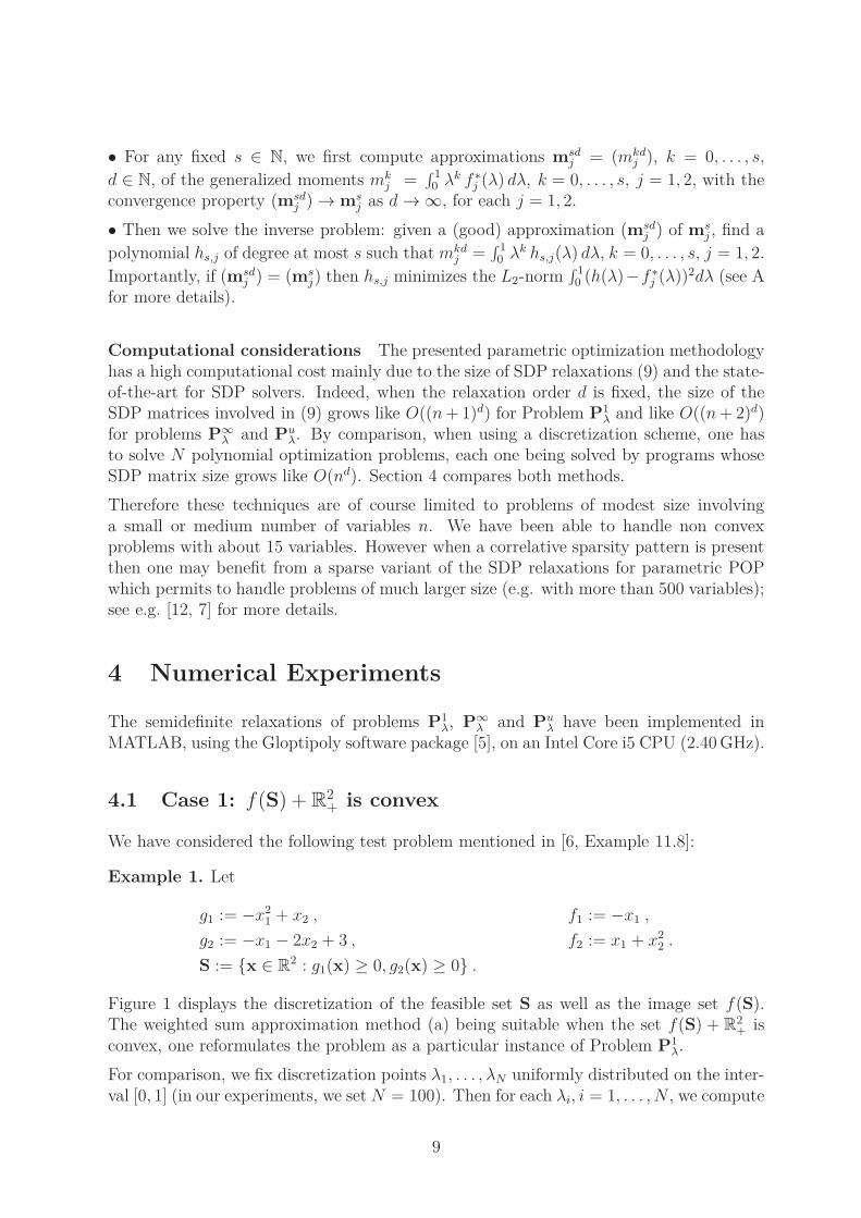
Example 1. Let

g1 := −x21 + x2 , f1 := −x1 ,

g2 := −x1 − 2x2 + 3 , f2 := x1 + x22 .

S := {x ∈ R2 : g1(x) ≥ 0, g2(x) ≥ 0} .

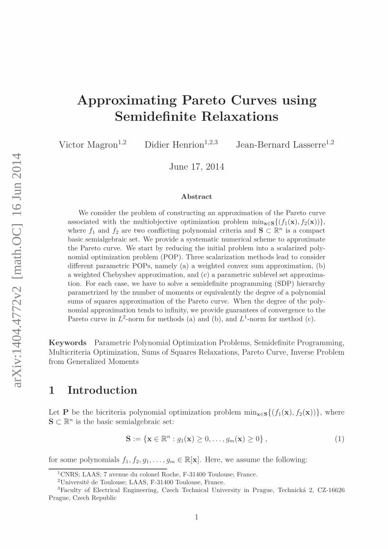
Figure 1 displays the discretization of the feasible set S as well as the image set f(S).The weighted sum approximation method (a) being suitable when the set f(S) + R

2+ is

convex, one reformulates the problem as a particular instance of Problem P1λ.

For comparison, we fix discretization points λ1, . . . , λN uniformly distributed on the inter-val [0, 1] (in our experiments, we set N = 100). Then for each λi, i = 1, . . . , N , we compute

9

−1.5 −1 −0.5 0 0.5 10

0.5

1

1.5

2

2.5

x1

x2

(a) S

−1.5 −1 −0.5 0 0.5 10

0.5

1

1.5

2

2.5

x1

x2

(b) f(S)

Figure 1: Preimage and image set of f for Example 1

the optimal value f ∗(λi) of the polynomial optimization problem P1λi

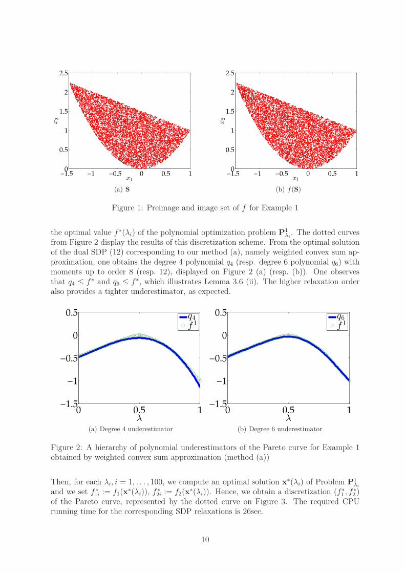
. The dotted curvesfrom Figure 2 display the results of this discretization scheme. From the optimal solutionof the dual SDP (12) corresponding to our method (a), namely weighted convex sum ap-proximation, one obtains the degree 4 polynomial q4 (resp. degree 6 polynomial q6) withmoments up to order 8 (resp. 12), displayed on Figure 2 (a) (resp. (b)). One observesthat q4 ≤ f ∗ and q6 ≤ f ∗, which illustrates Lemma 3.6 (ii). The higher relaxation orderalso provides a tighter underestimator, as expected.

0 0.5 1−1.5

−1

−0.5

0

0.5

λ

q4f 1

(a) Degree 4 underestimator

0 0.5 1−1.5

−1

−0.5

0

0.5

λ

q6f 1

(b) Degree 6 underestimator

Figure 2: A hierarchy of polynomial underestimators of the Pareto curve for Example 1obtained by weighted convex sum approximation (method (a))

Then, for each λi, i = 1, . . . , 100, we compute an optimal solution x∗(λi) of Problem P1λi

and we set f ∗1i := f1(x

∗(λi)), f ∗2i := f2(x∗(λi)). Hence, we obtain a discretization (f ∗

1 , f ∗2 )

of the Pareto curve, represented by the dotted curve on Figure 3. The required CPUrunning time for the corresponding SDP relaxations is 26sec.

10

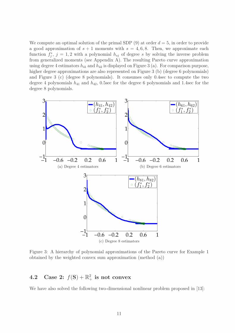
We compute an optimal solution of the primal SDP (9) at order d = 5, in order to providea good approximation of s + 1 moments with s = 4, 6, 8. Then, we approximate eachfunction f ∗

j , j = 1, 2 with a polynomial hsj of degree s by solving the inverse problemfrom generalized moments (see Appendix A). The resulting Pareto curve approximationusing degree 4 estimators h41 and h42 is displayed on Figure 3 (a). For comparison purpose,higher degree approximations are also represented on Figure 3 (b) (degree 6 polynomials)and Figure 3 (c) (degree 8 polynomials). It consumes only 0.4sec to compute the twodegree 4 polynomials h41 and h42, 0.5sec for the degree 6 polynomials and 1.4sec for thedegree 8 polynomials.

−1 −0.6 −0.2 0.2 0.6 1−1

0

1

2

3

(h41, h42)(f ∗

1 , f∗

2 )

(a) Degree 4 estimators

−1 −0.6 −0.2 0.2 0.6 1−1

0

1

2

3

(h61, h62)(f ∗

1 , f∗

2 )

(b) Degree 6 estimators

−1 −0.6 −0.2 0.2 0.6 1−1

0

1

2

3

(h81, h82)(f ∗

1 , f∗

2 )

(c) Degree 8 estimators

Figure 3: A hierarchy of polynomial approximations of the Pareto curve for Example 1obtained by the weighted convex sum approximation (method (a))

4.2 Case 2: f(S) + R2+ is not convex

We have also solved the following two-dimensional nonlinear problem proposed in [13]:

11

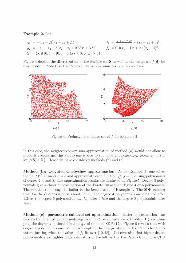
Example 2. Let

g1 := −(x1 − 2)3/2 − x2 + 2.5 , f1 := (x1+x2−7.5)2

4+ (x2 − x1 + 3)2 ,

g2 := −x1 − x2 + 8(x2 − x1 + 0.65)2 + 3.85 , f2 := 0.4(x1 − 1)2 + 0.4(x2 − 4)2 .

S := {x ∈ [0, 5] × [0, 3] : g1(x) ≥ 0, g2(x) ≥ 0} .

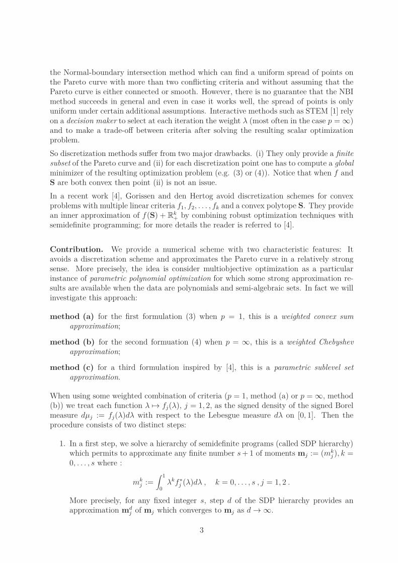
Figure 4 depicts the discretization of the feasible set S as well as the image set f(S) forthis problem. Note that the Pareto curve is non-connected and non-convex.

0 1.3 2.6 3.90

1

2

3

x1

x2

(a) S

0 20 40 600

2

4

6

y1

y2

(b) f(S)

Figure 4: Preimage and image set of f for Example 2

In this case, the weighted convex sum approximation of method (a) would not allow toproperly reconstruct the Pareto curve, due to the apparent nonconvex geometry of theset f(S) + R

2+. Hence we have considered methods (b) and (c).

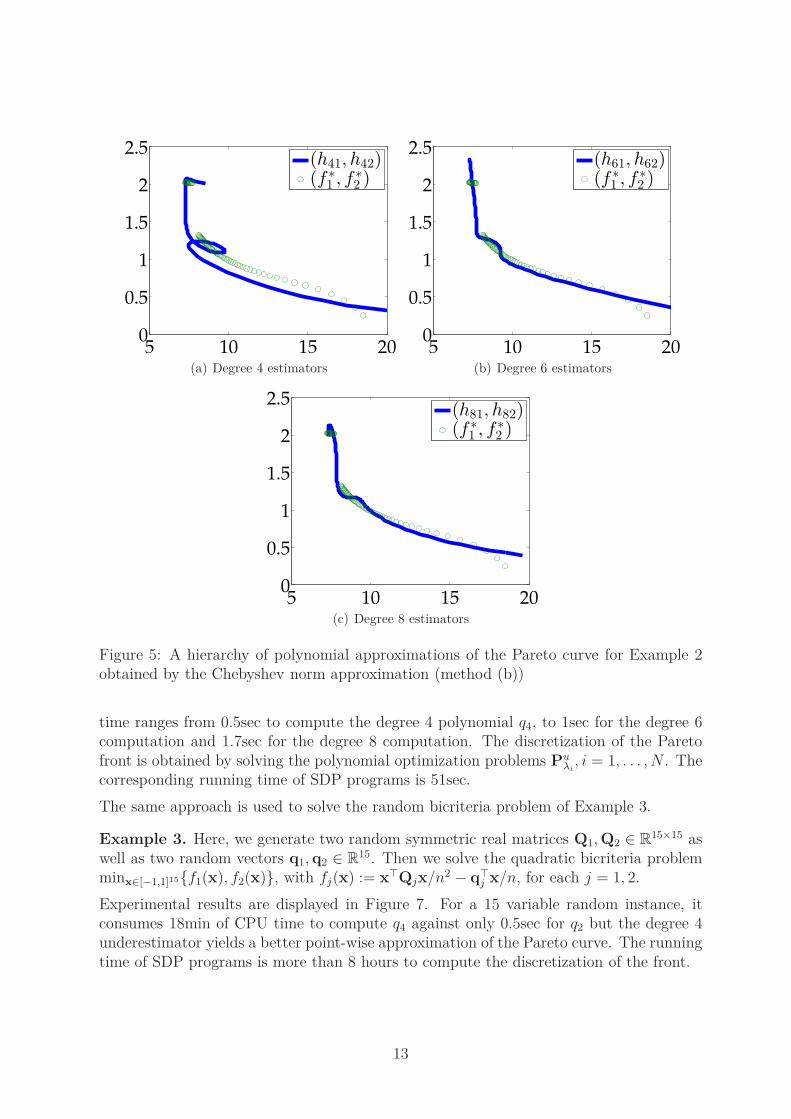
Method (b): weighted Chebyshev approximation As for Example 1, one solvesthe SDP (9) at order d = 5 and approximate each function f ∗

j , j = 1, 2 using polynomialsof degree 4, 6 and 8. The approximation results are displayed on Figure 5. Degree 8 poly-nomials give a closer approximation of the Pareto curve than degree 4 or 6 polynomials.The solution time range is similar to the benchmarks of Example 1. The SDP runningtime for the discretization is about 3min. The degree 4 polynomials are obtained after1.3sec, the degree 6 polynomials h61, h62 after 9.7sec and the degree 8 polynomials after1min.

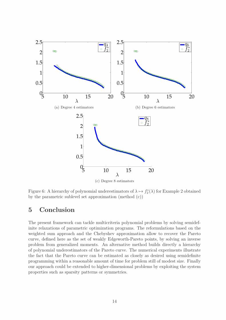
Method (c): parametric sublevel set approximation Better approximations canbe directly obtained by reformulating Example 2 as an instance of Problem Pu

λ and com-pute the degree d optimal solutions q2d of the dual SDP (12). Figure 6 reveals that withdegree 4 polynomials one can already capture the change of sign of the Pareto front cur-vature (arising when the values of f1 lie over [10, 18]). Observe also that higher-degreepolynomials yield tighter underestimators of the left part of the Pareto front. The CPU

12

5 10 15 200

0.5

1

1.5

2

2.5

(h41, h42)(f ∗

1 , f∗

2 )

(a) Degree 4 estimators

5 10 15 200

0.5

1

1.5

2

2.5

(h61, h62)(f ∗

1 , f∗

2 )

(b) Degree 6 estimators

5 10 15 200

0.5

1

1.5

2

2.5

(h81, h82)(f ∗

1 , f∗

2 )

(c) Degree 8 estimators

Figure 5: A hierarchy of polynomial approximations of the Pareto curve for Example 2obtained by the Chebyshev norm approximation (method (b))

time ranges from 0.5sec to compute the degree 4 polynomial q4, to 1sec for the degree 6computation and 1.7sec for the degree 8 computation. The discretization of the Paretofront is obtained by solving the polynomial optimization problems Pu

λi, i = 1, . . . , N . The

corresponding running time of SDP programs is 51sec.

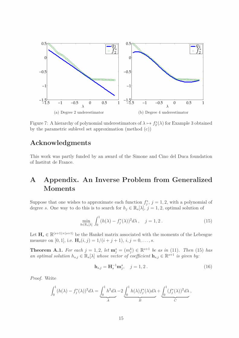
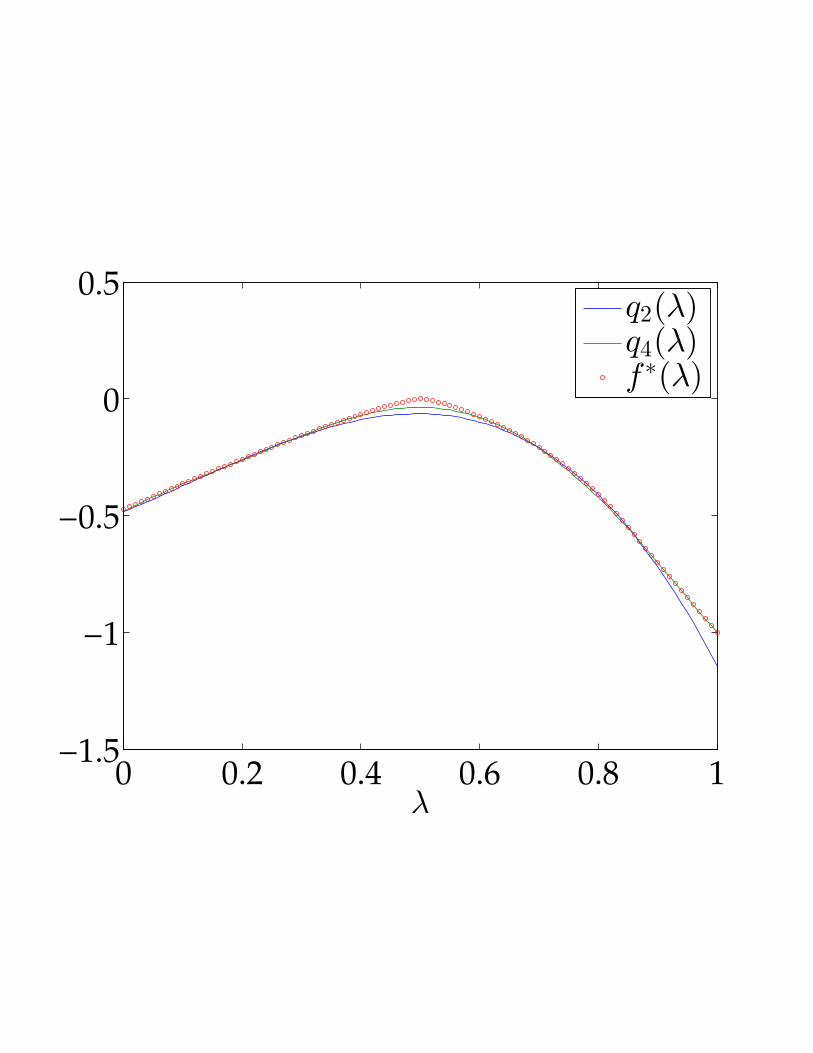
The same approach is used to solve the random bicriteria problem of Example 3.

Example 3. Here, we generate two random symmetric real matrices Q1, Q2 ∈ R15×15 as

well as two random vectors q1, q2 ∈ R15. Then we solve the quadratic bicriteria problem

minx∈[−1,1]15{f1(x), f2(x)}, with fj(x) := x⊤Qjx/n2 − q⊤j x/n, for each j = 1, 2.

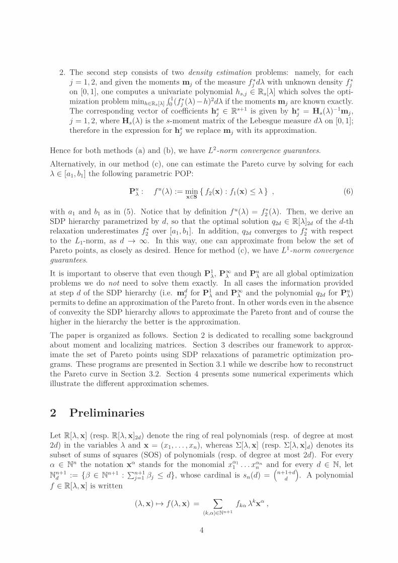
Experimental results are displayed in Figure 7. For a 15 variable random instance, itconsumes 18min of CPU time to compute q4 against only 0.5sec for q2 but the degree 4underestimator yields a better point-wise approximation of the Pareto curve. The runningtime of SDP programs is more than 8 hours to compute the discretization of the front.

13

5 10 15 200

0.5

1

1.5

2

2.5

λ

q4f ∗

2

(a) Degree 4 estimators

5 10 15 200

0.5

1

1.5

2

2.5

λ

q6f ∗

2

(b) Degree 6 estimators

5 10 15 200

0.5

1

1.5

2

2.5

λ

q8f ∗

2

(c) Degree 8 estimators

Figure 6: A hierarchy of polynomial underestimators of λ 7→ f ∗2 (λ) for Example 2 obtained

by the parametric sublevel set approximation (method (c))

5 Conclusion

The present framework can tackle multicriteria polynomial problems by solving semidef-inite relaxations of parametric optimization programs. The reformulations based on theweighted sum approach and the Chebyshev approximation allow to recover the Paretocurve, defined here as the set of weakly Edgeworth-Pareto points, by solving an inverseproblem from generalized moments. An alternative method builds directly a hierarchyof polynomial underestimators of the Pareto curve. The numerical experiments illustratethe fact that the Pareto curve can be estimated as closely as desired using semidefiniteprogramming within a reasonable amount of time for problem still of modest size. Finallyour approach could be extended to higher-dimensional problems by exploiting the systemproperties such as sparsity patterns or symmetries.

14

−1.5 −1 −0.5 0 0.5 1−1.5

−1

−0.5

0

0.5

λ

q2f ∗

2

(a) Degree 2 underestimator

−1.5 −1 −0.5 0 0.5 1−1.5

−1

−0.5

0

0.5

λ

q4f ∗

2

(b) Degree 4 underestimator

Figure 7: A hierarchy of polynomial underestimators of λ 7→ f ∗2 (λ) for Example 3 obtained

by the parametric sublevel set approximation (method (c))

Acknowledgments

This work was partly funded by an award of the Simone and Cino del Duca foundationof Institut de France.

A Appendix. An Inverse Problem from Generalized

Moments

Suppose that one wishes to approximate each function f ∗j , j = 1, 2, with a polynomial of

degree s. One way to do this is to search for hj ∈ Rs[λ], j = 1, 2, optimal solution of

minh∈Rs[λ]

∫ 1

0(h(λ) − f ∗

j (λ))2dλ , j = 1, 2 . (15)

Let Hs ∈ R(s+1)×(s+1) be the Hankel matrix associated with the moments of the Lebesgue

measure on [0, 1], i.e. Hs(i, j) = 1/(i + j + 1), i, j = 0, . . . , s.

Theorem A.1. For each j = 1, 2, let msj = (mk

j ) ∈ Rs+1 be as in (11). Then (15) has

an optimal solution hs,j ∈ Rs[λ] whose vector of coefficient hs,j ∈ Rs+1 is given by:

hs,j = H−1s ms

j , j = 1, 2 . (16)

Proof. Write

∫ 1

0(h(λ) − f ∗

j (λ))2dλ =∫ 1

0h2dλ

︸ ︷︷ ︸

A

−2∫ 1

0h(λ)f ∗

j (λ)dλ︸ ︷︷ ︸

B

+∫ 1

0(f ∗

j (λ))2dλ︸ ︷︷ ︸

C

,

15

and observe that

A = h⊤Hsh , B =s∑

k=0

hk

∫ 1

0λkf ∗

j (λ) dλ =s∑

k=0

hk mkj = h⊤mj ,

and so, as C is a constant, (15) reduces to

minh∈Rs+1

h⊤Hsh − 2h⊤mj , j = 1, 2 ,

from which (16) follows.

References

[1] R. Benayoun, J. Montgolfier, J. Tergny, and O. Laritchev. Linear programmingwith multiple objective functions: Step method (stem). Mathematical Programming,1(1):366–375, 1971.

[2] Indraneel Das and J. E. Dennis. Normal-boundary intersection: A new method forgenerating the pareto surface in nonlinear multicriteria optimization problems. SIAMJ. on Optimization, 8(3):631–657, March 1998.

[3] Gabriele Eichfelder. Scalarizations for adaptively solving multi-objective optimizationproblems. Comput. Optim. Appl., 44(2):249–273, November 2009.

[4] Bram L. Gorissen and Dick den Hertog. Approximating the pareto set of multiobjec-tive linear programs via robust optimization. Operations Research Letters, 40(5):319– 324, 2012.

[5] Didier Henrion, Jean-Bernard Lasserre, and Johan Lofberg. GloptiPoly 3: moments,optimization and semidefinite programming. Optimization Methods and Software,24(4-5):pp. 761–779, August 2009.

[6] J. Jahn. Vector Optimization: Theory, Applications, and Extensions. Springer, 2010.

[7] Jean B. Lasserre. Convergent sdp-relaxations in polynomial optimization with spar-sity. SIAM Journal on Optimization, 17(3):822–843.

[8] Jean B. Lasserre. Global optimization with polynomials and the problem of moments.SIAM Journal on Optimization, 11(3):796–817, 2001.

[9] Jean B. Lasserre. A “joint+marginal” approach to parametric polynomial optimiza-tion. SIAM Journal on Optimization, 20(4):1995–2022, 2010.

[10] K. Miettinen. Nonlinear Multiobjective Optimization, volume 12 of International Se-ries in Operations Research and Management Science. Kluwer Academic Publishers,Dordrecht, 1999.

16

[11] Elijah Polak. On the approximation of solutions to multiple criteria decision makingproblems. In Milan Zeleny, editor, Multiple Criteria Decision Making Kyoto 1975,volume 123 of Lecture Notes in Economics and Mathematical Systems, pages 271–282.Springer Berlin Heidelberg, 1976.

[12] Hayato Waki, Sunyoung Kim, Masakazu Kojima, and Masakazu Muramatsu. Sumsof squares and semidefinite programming relaxations for polynomial optimizationproblems with structured sparsity. SIAM Journal on Optimization, 17(1):218–242,2006.

[13] Benjamin Wilson, David Cappelleri, Timothy W. Simpson, and Mary Frecker. Ef-ficient Pareto Frontier Exploration using Surrogate Approximations. Optimizationand Engineering, 2(1):31–50, 2001.

17

0 0.2 0.4 0.6 0.8 1−1.5

−1

−0.5

0

0.5

λ

q2(λ)q4(λ)f∗(λ)