ApproximabilityofOptimizationProblemswithinan ... · ApproximabilityofOptimizationProblemswithinan...

CENTRO DE INVESTIGACIÓN Y DE ESTUDIOSAVANZADOS DEL INSTITUTO POLITÉCNICO NACIONAL

UNIDAD ZACATENCODEPARTAMENTO DE COMPUTACIÓN

Approximability of Optimization Problems within anApproach of Quantum Computing

A dissertation submitted by

William de la Cruz de los Santos

For the degree of

Doctor of Computer Science

Supervisor

Guillermo Morales Luna

México D.F. March 2013

CENTRO DE INVESTIGACIÓN Y DE ESTUDIOSAVANZADOS DEL INSTITUTO POLITÉCNICO NACIONAL

UNIDAD ZACATENCODEPARTAMENTO DE COMPUTACIÓN

Aproximación a problemas de optimización con unenfoque de cómputo cuántico

Tesis que presenta

William de la Cruz de los Santos

Para obtener el grado de

Doctor en Ciencias en Computación

Director de tesis:

Guillermo Morales Luna

México, D.F. Marzo de 2013

Abstract

Quantum Computing appeared about 30 years ago motivated by the ideas of RichardFeynman. He wondered whether it is possible to simulate a quantum system by meansof a universal quantum machine or quantum computer. Although, there is no yet apractical implementation of a quantum computer, researches have done impressivetheoretical results in the design of quantum algorithms, an important quantum algo-rithm is the Shor algorithm to factorize an integer number into its prime factors [76].A quantum algorithm has as input an initial state, and then a series of unitary ma-trices are applied over the initial state in order to produce a final state, the output ofthe algorithm is obtained by performing a quantum measurement over the final state.This kind of quantum algorithms belong to the Quantum Circuit Model (QCM) [61].

Recently, it was proposed the Adiabatic Quantum Computation (AQC) [37, 35]that is based on the Adiabatic Theorem [58, 42] to approximate solutions of theSchrödinger equation. The design of an AQC algorithm involves the construction ofa Hamiltonian that describes the behavior of the quantum system, this Hamiltonianis expressed as a linear interpolation of an initial Hamiltonian whose ground stateis easy to compute, and a final Hamiltonian whose ground state corresponds to thesolution of a given optimization problem. The Adiabatic Theorem asserts that if thetime evolution of a quantum system described by a Hamiltonian is large enough, thenthe system remains close to its ground state. Thus, given an optimization problem, anAQC algorithm uses the Adiabatic Theorem to approximate the ground state of thefinal Hamiltonian that corresponds to the solution of the given optimization problem.The time complexity of an AQC algorithm is the minimum time that satisfies theAdiabatic Theorem.

AQC has been used to solve optimization problems, in [35] the authors claim thatthe optimization problem MAX-SAT can be solved in polynomial time complexityby an AQC algorithm. In [2] it was proved that QCM is equivalent to AQC. Fromthe computational point of view it is important to compute the spectrum of theHamiltonian in an AQC algorithm along the integration time in order to estimate itstime complexity. In general, it is a hard problem to know the time complexity of anAQC algorithm.

We investigate the computational simulation of AQC algorithms for the MAX-SAT optimization problem, we propose a symbolic analysis of the AQC solution inorder to understand the involved computational complexity of the AQC algorithms.This approach can be extended to others combinatorial optimization problems. Thecomputational simulation of an AQC algorithm requires the construction of a matrixof dimension 2n×2n where n is the dimension of the quantum system, that in generalcorresponds to a sparse matrix, this matrix is constructed using matrix tensor prod-ucts. We propose an efficient construction of the Hamiltonian for AQC algorithmsthat avoid the matrix tensor products.

The design of AQC algorithms has important consequences in its time complexityand also for its possible physical implementation. In Quantum Mechanics it is con-

venient to describe a Hamiltonian as an addition of local Hamiltonians i.e., Hamil-tonians that only act on a subset of states in the quantum system. On the otherhand, the pseudo-Boolean optimization model has been used to model combinatorialoptimization problems into pseudo-Boolean maps. We propose a general scheme todesign AQC algorithms based on pseudo-Boolean maps for combinatorial optimiza-tion problems, and we show that for a given optimization problem expressed in thepseudo-Boolean optimization model, then it is possible to construct an AQC algo-rithm with local Hamiltonians.

In [47] it was proved that NP-problems can be expressed in Second Order Logic(SOL). In [27] it was shown that all instances of graph problems expressed in MonadicSecond Order Logic (MSOL) with bounded treewidth can be solved in polynomialtime complexity. The algorithmic solution proposed in [27] is based on a DynamicProgramming approach over tree-decompositions of graphs [13, 18]. We show thatevery MSOL expression has associated pseudo-Boolean maps that can be obtainedby expanding the given MSOL expression, and also can be reduced to quadraticforms. The equivalence between MSOL expressions and quadratic pseudo-Booleanmaps can be considered as a general scheme to design AQC algorithms, since everyquadratic pseudo-Boolean map can be optimized by an AQC algorithm. We also showa composition scheme for local Hamiltonians based on the dynamic programmingapproach over tree-decompositions of graphs.

Resumen

La Computación Cuántica apareció hace cerca de 30 años motivada por la ideas deRichard Feyman, quien se preguntaba si era posible simular un sistema cuántico pormedio de una máquina cuántica universal o computadora cuántica. Aunque todavía noexiste una implementación física de una computadora cuántica, se han hecho grandesprogresos teóricos en el diseño de algoritmos cuánticos, por ejemplo el algoritmo cuán-tico de Shor para factorizar números enteros en sus factores primos [76]. Un algoritmocuántico recibe como entrada un estado inicial, sobre el cual se aplican sucesivamentematrices unitarias, obteniendo así un estado final, la salida del algoritmo se obtienellevando a cabo una medición cuántica sobre el estado final. Este tipo de algoritmoscuánticos pertenecen al Modelo de Circuitos Cuánticos (MCC) [61].

Recientemente, se propuso la Computación Cuántica Adiabática (CCA) [37, 35]que se basa en el Teorema Adiabático [58, 42] para aproximar soluciones de la ecuaciónde Schrödinger. El diseño de un algoritmo en CCA involucra la construcción de unhamiltoniano que describe el comportamiento del sistema cuántico, este hamiltonianose expresa como una interpolación lineal de un hamiltoniano inicial cuyo estado firmesea fácil de calcular, y un hamiltoniano final cuyo estado firme corresponde a lasolución de un problema de optimización dado. El Teorema Adiabático establece quesi el tiempo de evolución de un sistema cuántico, descrito por un hamiltoniano, eslo suficientemente grande, entonces el sistema se mantiene cerca de su estado firme.Así, dado un problema de optimización, un algoritmo en CCA emplea el TeoremaAdiabático para aproximar el estado firme del hamiltoniano final, que corresponde ala solución del problema de optimización. Se considera a la complejidad en tiempode un algoritmo en CCA como al mínimo tiempo tal que se satisfaga el TeoremaAdiabático.

La CCA se ha empleado para resolver problemas de optimización, en [35] losautores creen que el problema MAX-SAT puede ser resuelto en complejidad de tiempopolinomial por un algoritmo en CCA. En [2] se probó que el MCC es equivalente ala CCA. Desde el punto de vista computacional, es importante calcular el espectrodel hamiltoniano a lo largo del tiempo de evolución de un algoritmo en CCA, estoayudaría a conocer su complejidad en tiempo. En general, conocer la complejidad entiempo de un algoritmo en CCA es un problema difícil [37].

Investigamos la simulación computacional de los algoritmos en CCA para el prob-lema de optimización MAX-SAT, proponemos un análisis simbólico de la solución enCCA con el fin de entender la complejidad computacional de los algoritmos en CCA.Este enfoque se puede extender a otros problemas de optimización combinatorios. Enla practica, la simulación computacional de un algoritmo en CCA requiere la con-strucción de una matriz de dimensión 2n × 2n donde n es la dimensión del sistemacuántico, en general esta matriz corresponde a una matriz dispersa, y se construyeusando el producto tensorial de matrices. Proponemos una construcción eficiente delos hamiltonianos en CCA para el problema MAX-SAT que evita el uso de productostensoriales.

El diseño de algoritmos en CCA tiene consecuencias en su complejidad en tiempo ytambién en su posible implementación física. En la Mecánica Cuántica es convenientedescribir un hamiltoniano como una suma de hamiltonianos locales i.e., hamiltoni-anos que actúan sobre un subconjunto de estados en el sistema cuántico. Por otrolado, el modelo de optimización de funciones pseudo-booleanas ha sido usado paramodelar problemas de optimización combinatorios por medio de funciones pseudo-booleanas. Proponemos un esquema general para el diseño de algoritmos en CCA pormedio de funciones pseudo-booleanas para problemas de optimización combinatorios.Probamos que para cada problema de optimización que se exprese en el modelo deoptimización de funciones pseudo-booleanas, se puede diseñar un algoritmo en CCAcon hamiltonianos locales.

En Complejidad Descriptiva la clase de problemas NP se puede describir comoexpresiones en la Lógica de Segundo Orden (LSO) [47]. En [27] se demuestra que to-das las instancias de problemas sobre gráficas que se expresan en la Lógica Monádicade Segundo Orden (LMSO) con ancho de árbol acotado, se pueden resolver en com-plejidad de tiempo polinomial. La solución algorítmica propuesta en [27] se basaen un esquema de programación dinámica sobre descomposiciones en árbol de grá-ficas [13, 18]. Demostramos que cada expresión en LMSO tiene asociada funcionespseudo-booleanas que se obtienen expandiendo la expresión en LMSO, y que se puedenreducir a formas cuadráticas. Esta equivalencia entre expresiones en LMSO y fun-ciones cuadráticas pseudo-booleanas se puede considerar como un esquema generalpara diseñar algoritmos en CCA, ya que cada función cuadrática pseudo-booleanapuede ser optimizada por un algoritmo en CCA. Mostramos también un esquemade composición de hamiltonianos locales que se basa en el enfoque de programacióndinámica sobre descomposiciones en árbol de gráficas.

Agradecimientos

Deseo agradecer sinceramente a mi asesor, al Dr. Guillermo Morales Luna poraceptar dirigir el presente trabajo y compartir sus conocimientos, así como su granmotivación en la investigación. Agradezco al Dr. Alán Aspuru-Guzik de la Universi-dad de Harvard, al Dr. Micho Durdevich Lucich del Instituto de Matemáticas en laUniversidad Nacional Autónoma de México, y a los doctores Debrup Chakraborty ySergio Víctor Chapa Vergara, ambos del CINVESTAV-IPN, por aceptar ser revisoresde este trabajo, y por sus valiosos comentarios y observaciones.

A mis padres, les agradezco su apoyo y motivación por inculcarme los ideales yprincipios que rigen mi vida.

Sin dejar de lado a mis amigos y compañeros, les quiero dar las gracias por susconsejos y porque aún y cuando las distancias son largas siempre están ahí para darconsejos y nuevas ideas.

También agradezco al personal secretarial del departamento de Computación,Sofia Reza, Felipa Rosas y Erika Ríos por su valioso e incondicional apoyo en di-versos trámites administrativos.

Agradezco al CONACyT por la beca otorgada durante la realización de estos estu-dios de doctorado, y muy especialmente al CINVESTAV por ofrecerme un ambiénteacadémico de calidad y excelencia.

Contents

1 Introduction 1

2 Approximability of NP-hard problems 52.1 Basic definitions . . . . . . . . . . . . . . . . . . . . . . . . . . . . . . 52.2 Probabilistic proof systems . . . . . . . . . . . . . . . . . . . . . . . . 62.3 Optimization problems . . . . . . . . . . . . . . . . . . . . . . . . . . 7

2.3.1 Approximation algorithms . . . . . . . . . . . . . . . . . . . . 82.4 Randomized classes . . . . . . . . . . . . . . . . . . . . . . . . . . . . 8

2.4.1 Quantum complexity . . . . . . . . . . . . . . . . . . . . . . . 9

3 Adiabatic quantum computing 113.1 Basic definitions . . . . . . . . . . . . . . . . . . . . . . . . . . . . . . 11

3.1.1 Linear operators . . . . . . . . . . . . . . . . . . . . . . . . . 123.2 Quantum states and evolution . . . . . . . . . . . . . . . . . . . . . . 143.3 The Adiabatic Theorem . . . . . . . . . . . . . . . . . . . . . . . . . 15

3.3.1 Adiabatic evolution . . . . . . . . . . . . . . . . . . . . . . . . 153.3.2 Quantum computation by adiabatic evolution . . . . . . . . . 16

3.4 Adiabatic paths . . . . . . . . . . . . . . . . . . . . . . . . . . . . . . 173.4.1 Geometric Berry phases . . . . . . . . . . . . . . . . . . . . . 193.4.2 Geometric quantum computation . . . . . . . . . . . . . . . . 21

4 Efficient Hamiltonian construction 234.1 AQC applied to the MAX-SAT problem . . . . . . . . . . . . . . . . 23

4.1.1 Satisfiability Problem . . . . . . . . . . . . . . . . . . . . . . . 244.1.2 AQC formulation of SAT . . . . . . . . . . . . . . . . . . . . . 24

4.2 Procedural Hamiltonian construction . . . . . . . . . . . . . . . . . . 274.2.1 Hyperplanes in the hypercube . . . . . . . . . . . . . . . . . . 274.2.2 The Hamiltonian operator HE . . . . . . . . . . . . . . . . . . 284.2.3 The Hamiltonian operator HZφ . . . . . . . . . . . . . . . . . 30

5 AQC for pseudo-Boolean optimization 335.1 Basic transformations . . . . . . . . . . . . . . . . . . . . . . . . . . 335.2 AQC for quadratic pseudo-Boolean maps . . . . . . . . . . . . . . . . 36

5.2.1 Hadamard transform . . . . . . . . . . . . . . . . . . . . . . . 37

xi

5.2.2 σx transform . . . . . . . . . . . . . . . . . . . . . . . . . . . . 395.3 k-local Hamiltonian problems . . . . . . . . . . . . . . . . . . . . . . 40

5.3.1 Reduction of graph problems to the 2-local Hamiltonian problem 425.4 Graph structures and optimization problems . . . . . . . . . . . . . . 44

5.4.1 Relational signatures . . . . . . . . . . . . . . . . . . . . . . . 445.4.2 First order logic . . . . . . . . . . . . . . . . . . . . . . . . . . 455.4.3 Second order logic . . . . . . . . . . . . . . . . . . . . . . . . 455.4.4 Monadic second-order logic decision and optimization problems 465.4.5 MSOL optimization problems and pseudo-Boolean maps . . . 47

6 A general strategy to solve NP-hard problems 536.1 Background . . . . . . . . . . . . . . . . . . . . . . . . . . . . . . . . 53

6.1.1 Basic notions . . . . . . . . . . . . . . . . . . . . . . . . . . . 536.1.2 Tree decompositions . . . . . . . . . . . . . . . . . . . . . . . 56

6.2 Procedural modification of tree decompositions . . . . . . . . . . . . . 566.2.1 Modification by the addition of an edge . . . . . . . . . . . . . 576.2.2 Iterative modification . . . . . . . . . . . . . . . . . . . . . . . 586.2.3 Branch decompositions . . . . . . . . . . . . . . . . . . . . . . 596.2.4 Comparison of time complexities . . . . . . . . . . . . . . . . 61

6.3 A strategy to solve NP-hard problems . . . . . . . . . . . . . . . . . 616.3.1 Dynamic programming approach . . . . . . . . . . . . . . . . 626.3.2 The Courcelle Theorem . . . . . . . . . . . . . . . . . . . . . . 636.3.3 Examples of second order formulae . . . . . . . . . . . . . . . 636.3.4 Dynamic Programming applied to NP-hard problems . . . . . 656.3.5 The Classical Ising model . . . . . . . . . . . . . . . . . . . . 676.3.6 Quantum Ising model . . . . . . . . . . . . . . . . . . . . . . . 70

7 Conclusions and future work 73

Appendix 75

References 77

List of Figures

2.1 Probabilistic Turing machine (verifier). . . . . . . . . . . . . . . . . . 7

3.1 Parallel transport of a vector without local rotation on a curved surface(in a sphere). The final vector vf has been rotated with respect to theinitial vector vi, and the rotation angle being the solid angle enclosedby the loop. . . . . . . . . . . . . . . . . . . . . . . . . . . . . . . . . 22

xiii

List of Tables

2.1 Randomized class of languages. . . . . . . . . . . . . . . . . . . . . . 9

xv

Chapter 1

Introduction

The first idea to perform computations using a quantum computer was proposed byRichard Feynman in 1982. He wondered whether it is possible to simulate a quantumsystem by means of a universal quantum simulator [38]. The Feynman’s proposalwas the initial motivation for many future experimental and theoretical results in thefield of Quantum Computation (QC).

The first important theoretical result was given in [76], it is proposed a polynomialtime quantum algorithm to the problem of factoring an integer number into its primefactors, that is believed to be a hard problem.

Since then, many quantum algorithms were proposed, for instance in [43] a sub-linear time quantum algorithm is given to solve the problem of finding an element ina non-structured database.

Quantum algorithms (QA) are based on the application of unitary operators thatact in a finite dimensional Hilbert space. Thus, a QA consists of consecutive ap-plications of unitary operators over an initial quantum state, and the output of thealgorithm is obtained by performing a quantum measurement over the final state.This approach is known as the quantum circuit model (QCM) (see [61]).

On other hand, Adiabatic Quantum Computation (AQC) was introduced in [37]and it has been applied to solve optimization problems. It is based in the construc-tion of a time-dependent Hamiltonian which codify the optimal solution of the givenoptimization problem into its ground state (see chapter 3). AQC makes use of theAdiabatic Theorem (see [58, 42]) to approximate solutions of the Schrödinger equationin which a slow evolution occurs.

Although, AQC approach is defined by the solutions of the continuous Schrödingerequation, it has been proved that AQC is equivalent to QCM (see [2]), and thereforeAQC is a universal model of computation.

A very active area in AQC deals with the problem to determine a time lower-bound that an AQC algorithm requires in order to obtain an optimal solution. In [37]an AQC algorithm was proposed for the 3-SAT problem (see chapter 4), and it isclaimed by means of simulations that the time required for the AQC algorithm scalepolynomially with the input size.

The Hamiltonian operators used in AQC should be local for convenience. Local

1

2 CHAPTER 1. INTRODUCTION

Hamiltonian operators are expressed as a polynomial sum i.e. the addition of a poly-nomial number of Hamiltonians each acting over a reduced number of states. Withthe use of local Hamiltonians, it is possible to perform computations in a local way,affecting only a neighborhood of states in the quantum system. A related impor-tant problem is the Local Hamiltonian Problem (LHP) that consists in deciding if agiven Hamiltonian acting in a Hilbert space of dimension n has an eigenvalue belowa, or if all its eigenvalues are at less b, where a and b are real numbers such thatb− a ≥ n−O(1).

The LHP is known to be QMA-complete (see [52, 51, 50, 22]) where QMA is theclass of problems that can be solved in polynomial time by QA’s. From the point ofview of complexity theory, the LHP can be seen as the quantum analog of the SATproblem for the class of problems NP and restricted versions of the LHP coincidewith NP-complete problems [83].

In [1] a general technique was proposed to decompose a Hamiltonian into a polyno-mial sum of local Hamiltonians, it is based on the assumption that the given Hamilto-nian is d-sparse and row-computable. The Hamiltonian decomposition it is importantto the Hamiltonian simulation which consists in computing the matrix exponentiationof a given Hermitian matrix that results into a unitary matrix (see [23, 12, 65]).

Formally, the Adiabatic Theorem guaranties that the final ground state of a givenHamiltonian can be approximated with arbitrary uncertainty, and assuming thatQC cannot solve NP-complete problems it follows that AQC is a means to obtainan approximation to the ground state and the ground state energy. The ratio ofthis approximation and its dependence on the hardness of the problem are not wellunderstood yet. On the other hand, classical algorithms have been proposed, forinstance, in [9] it was shown a classical approximation algorithm for evaluating theground-state energy of the classical Ising Hamiltonian with linear terms on an arbi-trary planar graph. Also, a classical approximation algorithm is proposed to the LHP(also see [62]).

The current construction of local Hamiltonians does not use the structure of thegiven problem. For instance, in [35] an adiabatic quantum algorithm is given forthe MAX-SAT problem. It is based on a natural equivalence between clauses andHamiltonians defined for every literal in the given instance. A similar construction isgiven in [66] for the protein folding problem, it is based on the Ising model to describethe local interactions in a lattice.

The design and construction of Hamiltonians have important consequences inthe running time and convergence for AQC algorithms (see [36, 79, 3, 25]). In thisthesis we deal with the problem of local Hamiltonian construction for combinatorialoptimization problems. Also, we investigate the classical simulation of the AQC forthe MAX-SAT problem. An important challenge in AQC is to propose new techniquesto codify a given problem into the Hamiltonian approach, for instance, the DynamicProgramming approach is a well known technique to solve NP-hard problems andhas been the basis for many polynomial time algorithms applied to graph problems(see [19, 13, 18]).

3

The main contributions of this thesis are the following:

• The first contribution is a complete analysis of the AQC applied to the 3-SAT problem, we analyze the syntactical construction of the initial and finalHamiltonians involved in the AQC algorithm, such as analysis is useful in orderto perform numerical simulations of the AQC algorithm i.e. to avoid a directconstruction of the Hamiltonians by means of tensor products. Also, we providea precise description of the computational complexity of the AQC algorithm.

• The second contribution is a general model in terms of pseudo-Boolean functionsto solve optimization problems. The main idea is to model any combinatorialoptimization as a quadratic pseudo-Boolean function [21], then a Hamiltonianoperator is constructed such that its ground state correspond to the point thatminimizes the quadratic pseudo-Boolean function. We also, show that anyproblem expressed in monadic second-order logic has an associated pseudo-Boolean function with a bounded number of variables.

• The last contribution of this thesis is a Dynamic Programming approach to solveNP-hard problems. It is based on the Tree Decompositions of graphs introducedin [69, 70, 71, 68] and a dynamic programming technique in which a graphproblem can be decomposed into smallest subproblems and then composed inorder to construct a global solution of the problem (see [13, 18]). Based onthis decomposition, we propose the Hamiltonian construction for AQC on eachsubproblem of the tree decomposition and composed in a global Hamiltonianwhose ground state is the point at with the pseudo-Boolean function has itsminimum.

The organization of this thesis is as follows: In chapter 2 a succinct introduc-tion to computational complexity is given, the basic definitions of complexity classesand optimization problems are introduced. In chapter 3 we give an introduction toadiabatic quantum computing. It is intended to be self-contained. In chapter 4 weexplore the classical simulation of the AQC for the MAX-SAT problem, we proposea symbolic analysis of the construction of Hamiltonias for AQC. In chapter 5 we givea general Hamiltonian construction for the pseudo-Boolean optimization problem. Inchapter 6 we show an alternative construction of local Hamiltonians based on a studyof graph decompositions and a dynamic programming approach. Finally, in chapter7 we have the conclusions and further research.

4 CHAPTER 1. INTRODUCTION

Chapter 2

Approximability of NP-hard problems

The purpose of this chapter is to give a succinct introduction to computational com-plexity and its principal problems, the scope of this review ranges from complexityclasses to approximating optimization problems. In the background, the knowledgeof Turing machines (TM) is assumed (see [8, 40, 6]).

We emphasize the relationship between decision and optimization problems. Inorder to do this, we recall the class P in terms of Deterministic Turing Machines(DTM) and the class NP in terms of DTM’s that test membership in languages.

The class NP has a probabilistic characterization in terms of Probabilistic TuringMachines (PTM), captured in the PCP theorem. The PCP theorem has impor-tant applications in approximating solutions to NP-hard problems using a standardmethodology.

We also introduce the randomized complexity classes and their connections withoptimization problems. Randomized computation is related to quantum computationby its probabilistic nature, that is, the quantum complexity class BQP contains theclassical complexity class BPP. Here we make a survey of these notions.

2.1 Basic definitionsLet L be a language. There exists a DTM M that recognizes L whenever L isdecidable. Given a DTM M , let LM be the language recognized by M . M is saidto be polynomial-time, if for each input string x, with |x| = n, M performs at mostO(nk) computing steps for a fixed non-negative exponent k, where |x| denote thelength of the string x.

Definition 1. The class P consists of all languages recognized by polynomial timeDTM’s.

Let L be a language, a verification procedure for L is a DTM V that satisfies thefollowing conditions:

1. Completeness: For each x ∈ L there exists a string y such that V (x, y) = 1.(V accepts y as a valid proof for the membership of x in L)

5

6 CHAPTER 2. APPROXIMABILITY OF NP-HARD PROBLEMS

2. Soundness: For each x /∈ L and every string y it holds that V (x, y) = 0.(V rejects y as proof for the membership of x in L)

A language L has an efficiently verifiable proof system if there exists a polynomial pand a polynomial time verification procedure V such that, for each x ∈ L : (∃y : |y| ≤p(|x|)∧V (x, y) = 1) and for every x /∈ L and every y, the equation V (x, y) = 0 holds.

Definition 2. The class NP consists of all languages that have efficient verifiableproof systems.

Hence, P ⊆ NP.Although the definition of the classes P and NP have been expressed in terms of

decision problems, there exist equivalent definitions for search problems.A search problem is a relation R ⊆ 0, 1∗ × 0, 1∗. For an instance x of R,

let R(x) := y : (x, y) ∈ R be the set of solutions of x. A function f : 0, 1∗ →0, 1∗ ∪ ⊥ solves the search problem R if for every x, whenever R(x) 6= ∅ we havef(x) ∈ R(x), otherwise f(x) = ⊥.

Let L1, L2 be two languages, L1 is reducible to L2 if there exists a function Φ :L1 → L2 such that, x ∈ L1 if and only if Φ(x) ∈ L2. The language L1 is said to bepolynomially reducible to L2 if the reduction map Φ can be computed in polynomialtime. In this case, it is written L1 ≤p L2.

A language L ∈ NP is NP-complete if for each L′ ∈ NP, L′ ≤p L. The NP-complete problems are thus the most difficult problems in the class NP.

2.2 Probabilistic proof systems

A verification procedure given by a DTM M can be extended by changing M witha PTM that uses a source of random bits for its computation. From now on, averification procedure will be called a verifier for short.

Definition 3. A verifier V is a PTM having an input tape, a work tape, a source ofrandom bits and a read-only tape called proof string π. V has random access to π andthe operation of reading a bit in π is called a query.

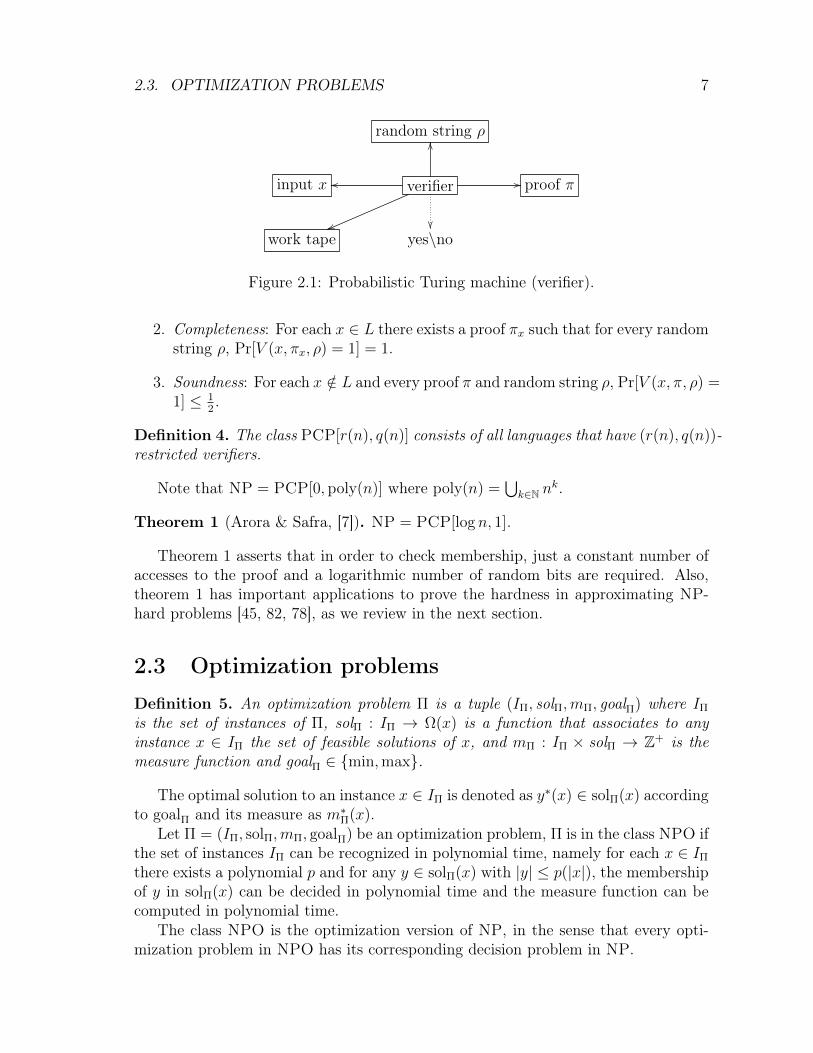
The source of random bits of a verifier can be viewed as an input random stringρ. The figure 2.1 shows a verifier and its components: It can be seen that a verifieris equivalent to a verification procedure when the verifier does not use the randomstring for its computation.

Let L be a language and q, r : N → N be two functions. L has a (r(n), q(n))-restricted verifier if there is a verifier V such that satisfies the following conditions:

1. Efficiency: For each input x with |x| = n and given a proof string π of lengthat most q(n)2r(n), V uses at most r(n) random bits and queries at most q(n)positions in π. Then V outputs 1 for “accept” or outputs 0 for “reject”.

2.3. OPTIMIZATION PROBLEMS 7

random string ρ

input x verifier

vv

oo //

OO

proof π

work tape yes\no

Figure 2.1: Probabilistic Turing machine (verifier).

2. Completeness: For each x ∈ L there exists a proof πx such that for every randomstring ρ, Pr[V (x, πx, ρ) = 1] = 1.

3. Soundness: For each x /∈ L and every proof π and random string ρ, Pr[V (x, π, ρ) =1] ≤ 1

2.

Definition 4. The class PCP[r(n), q(n)] consists of all languages that have (r(n), q(n))-restricted verifiers.

Note that NP = PCP[0, poly(n)] where poly(n) =⋃k∈N n

k.

Theorem 1 (Arora & Safra, [7]). NP = PCP[log n, 1].

Theorem 1 asserts that in order to check membership, just a constant number ofaccesses to the proof and a logarithmic number of random bits are required. Also,theorem 1 has important applications to prove the hardness in approximating NP-hard problems [45, 82, 78], as we review in the next section.

2.3 Optimization problems

Definition 5. An optimization problem Π is a tuple (IΠ, solΠ,mΠ, goalΠ) where IΠ

is the set of instances of Π, solΠ : IΠ → Ω(x) is a function that associates to anyinstance x ∈ IΠ the set of feasible solutions of x, and mΠ : IΠ × solΠ → Z+ is themeasure function and goalΠ ∈ min,max.

The optimal solution to an instance x ∈ IΠ is denoted as y∗(x) ∈ solΠ(x) accordingto goalΠ and its measure as m∗Π(x).

Let Π = (IΠ, solΠ,mΠ, goalΠ) be an optimization problem, Π is in the class NPO ifthe set of instances IΠ can be recognized in polynomial time, namely for each x ∈ IΠ

there exists a polynomial p and for any y ∈ solΠ(x) with |y| ≤ p(|x|), the membershipof y in solΠ(x) can be decided in polynomial time and the measure function can becomputed in polynomial time.

The class NPO is the optimization version of NP, in the sense that every opti-mization problem in NPO has its corresponding decision problem in NP.


A problem Π is NP-hard if there exists an NP-complete problem Π′ such thatΠ′ ≤T,p Π where ≤T,p is a polynomial Turing reduction (See [8]).

The NP-hard problems are the most difficult problems in NPO.

2.3.1 Approximation algorithms

Let Π be an optimization problem, for any x ∈ IΠ and for any value y ∈ solΠ(x), theperformance ratio of y with respect to x is defined as:

R(x, y) = max

mΠ(x, y)

m∗Π(x),m∗Π(x)

mΠ(x, y)

,

the performance ratio is always a number greater than or equal to 1 and is closer to1 as y is closer to the optimum solution.

An algorithm T is an ε-approximation algorithm for Π if, given any x ∈ IΠ,R(x, T (x)) ≤ ε, and it is said that Π is ε-approximated.

APX is the class of all NPO problems Π such that, for some ε > 1, there existsa polynomial time ε-approximation algorithm for Π.

Let Π be an NPO problem. An algorithm T is said to be an approximation schemefor Π if, for any x ∈ IΠ and for any rational ε > 1, T (x, ε) returns a feasible solutionof x whose performance ratio is at most ε.

Definition 6. An NPO problem Π belongs to the class PTAS if it admits a polynomial-time approximation scheme.

Note that the time complexity of an approximation scheme may be of the type21/(ε−1)p(|x|) or |x|1/(ε−1) where p is a polynomial.

An NPO problem Π belongs to the class FPTAS if it admits a fully polynomial-time approximation scheme, that is, an approximation scheme whose time complexityis bounded by q(|x|, 1/(ε− 1)) where q is a polynomial.

Clearly, FPTAS ⊆ PTAS ⊆ Apx ⊆ NPO.

2.4 Randomized classes

In previous sections a PTM was introduced and considered as a verifier, here a PTMis used to compute functions in a general setting.

Let L be a language, L has a polynomial-time PTMM if there exists a polynomialp such that, for each x ∈ L, M(x) can be computed within at most p(|x|) steps. Forany x ∈ L, M(x) is a random variable over the output distribution of M with inputx. Note that, if x ∈ L then M may fail to give the answer M(x) = 1 with input x.

The types of failures of a PTMM for a language L can be characterized as follows:

1. Two-sided error: M can fail in both directions, i.e., if x ∈ L, M may rule thatM(x) = 0, and conversely.

2.4. RANDOMIZED CLASSES 9

Type of error Class x ∈ L x /∈ L ⊥Two-sided BPP Pr[M(x) = 1] ≥ 2

3Pr[M(x) = 0] ≥ 2

3

One-sided RP Pr[M(x) = 1] ≥ 12

Pr[M(x) = 0] = 1Zero-sided ZPP Pr[M(x) = 1] = 1, Pr[M(x) = 0] = 1, Pr[M(x) = ⊥] = 1

Pr[M(x) = 1] ≥ 12

Pr[M(x) = 0] ≥ 12

Table 2.1: Randomized class of languages.

2. One-sided error: M can fail in one direction, i.e., if x /∈ L, M may rule thatM(x) = 1, but if x ∈ L, M(x) = 1.

3. Zero-sided error: M does not fail to recognize an element in L and is able toindicate its failure to find an answer.

The table 2.1 shows the classes of languages L that can be recognized by polynomial-time PTM’s M with respect to the type of failure defined before:

The symbol “⊥” is the output of a PTM when fails to give an answer.Formally the class ZPP is defined as follows: A language L is in ZPP if there

exists a PTM M such that Pr[M(x) ∈ χL(x),⊥] = 1 and Pr[M(x) ∈ χL(x)] ≥ 12

where χL(x) = 1 if x ∈ L and χ(x) = 0 if x /∈ L.It is easy to prove that RP ⊆ NP and RP ⊆ BPP.A PTM can approximate solutions of a NP-hard problem considering their corre-

sponding decision problem: Let Π = (IΠ, solΠ,mΠ, goalΠ) be an optimization problem.Given x ∈ IΠ and an integer k ∈ Z+, the decision problem ΠD with respect to Π isthe following: decide whether m∗Π(x) ≥ k if goalΠ = MAX or whether m∗Π(x) ≤ kif goalΠ = min. Finally, the language with respect to ΠD is LΠ = (x, k)|x ∈IΠ ∧m∗Π(x) ≥ k if goalΠ = max.

2.4.1 Quantum complexity

Quantum computation is realized in finite dimensional Hilbert spaces, the operationsare realized as unitary operators over unit vectors represented as linear combinationsof vectors in an orthonormal basis. Quantum measurements are the operations ofreading the results. The notion of Quantum algorithms were first introduced in [11]using Quantum Turing Machines (QTM), which extend the classical TM.

Formally, a QTM is a triplet (Σ, Q, δ) where Σ is a finite alphabet, Q is a finiteset of states with an distinguished initial state q0, a final state qf , and δ a quantumtransition function

δ : Q× Σ→ CQ×Σ×L,R

where L,R is a left or right displacement over the tape machine and C is a set ofcomputable complex numbers within some precision.

The QTM has a two-way infinite tape of cells indexed by Z and a single red/writetape head that moves along the tape. Given a pair (q, s) ∈ Q × Σ, δ associates a


complex number α ∈ C to (q, s), such that the absolute value of α is the probabilitythat the QTM will be in the new configuration (q′, s′) performing a left or rightdisplacement over the tape machine.

A QTM halts if reaches the final configuration with state qf , and it is said tobe polynomial time if it performs a polynomial number of states transitions. It ispossible to define an inner-product S space over C as the space of configurations of aQTM with the Euclidean norm, in this way, a linear combination of states in S is asuperposition of states of a QTM.

A QTMM recognizes exactly the language L, if for each x ∈ L, M accepts x withprobability 1 and for each x /∈ L, M rejects x with probability 1.

The class EQP consists of all languages recognized exactly by polynomial timeQTM’s.

A QTM M recognizes the language L with probability p if for each x ∈ L, Maccepts x with probability p and for each x /∈ L, M rejects x with probability 1− p.

Definition 7. The class BQP consists of all languages that are recognized by poly-nomial time QTM’s with probability 2

3.

The zero-sided error version of BQP is the class ZQP defined as follows: Alanguage L is in ZQP if for every x ∈ L, x is accepted by some polynomial time QTMwith probability 2

3and rejected with probability 0, and for every x /∈ L, x is rejected

by some polinomial time QTM with probability 23and accepted with probability 0.

Hence, EQP ⊆ ZQP ⊆ BQP.The known relations with classical complexity classes are: P ⊆ BQP, BPP ⊆

BQP and BQP ⊆ PSPACE [61].

Chapter 3

Adiabatic quantum computing

This chapter is a self-contained introduction to adiabatic quantum computing (AQC)as a general approach to solve optimization problems.

The first part is dedicated to recall the basic notions of Hilbert spaces and theirmetrics. The linear operators are introduced and their properties in the evolution ofQuantum Systems using the Schrödinger picture.

Also, a brief terminology with Quantum Mechanics is given, in order to definestates, observables, measurements and dynamics of a quantum system. An importantpart of this chapter is the exposition of the Adiabatic Theorem, which is the funda-mental tool in AQC. We sketch the general algorithm for AQC to solve optimizationproblems (see [37]).

Finally, we analyze the conditions in which the Adiabatic Theorem is satisfiedand the influence of the geometric Berry phases in the evolution of the adiabaticpaths (see [42]).

3.1 Basic definitionsA metric space is a pair (M,d) where M is a non-empty set and d : M ×M → R+ isa metric on M satisfying ∀x, y, z ∈M :

1. d(x, y) ≥ 0, and d(x, y) = 0 if and only if x = y,

2. d(x, y) = d(y, x),

3. d(x, y) ≤ d(x, z) + d(z, y).

A metric space M is complete if every Cauchy sequence converges in M .If V is any vector space then, the elements of V will be written using bold lowercase

letters as x,y, z. Any complex vector space V with induced norm by the inner productis a metric space with metric defined as d(x,y) = ‖x− y‖ for all x,y ∈ V .

Let 〈·|·〉 : V × V → C be an inner product thus, for all x,y, z ∈ V, a, b ∈ C:

1. 〈x|y〉 ≥ 0 and the following holds 〈x|y〉 = 0 if and only if x = y,

11

12 CHAPTER 3. ADIABATIC QUANTUM COMPUTING

2. 〈x|ay + bz〉 = a 〈x|y〉+ b 〈x|z〉,

3. 〈x|y〉 = 〈y|x〉∗.

The induced norm of a complex vector space V is defined as ‖x‖ = 〈x|x〉12 with

x ∈ V , and for any x,y ∈ V, a ∈ C,

1. ‖x‖ ≥ 0, and ‖x‖ = 0 if x = 0,

2. ‖x + y‖ ≤ ‖x‖+ ‖y‖,

3. ‖ax‖ = |a|‖x‖.

Definition 8. A Hilbert space is a complex vector space H with inner product whichis complete with respect to the metric induced by the inner product.

Let H1 = C2 be the complex Hilbert space of dimension 2. Let, for each n > 1,Hn = Hn−1⊗H1 be the n-fold tensor product of H1. Hn is a Hilbert space of dimensionN = 2n, and for any x ∈ Hn : x = (x0, . . . , xN−1) is a vector with N complex entries.

For any two integers i, j ∈ N, i ≤ j, let [[i, j]] denote the collection of integersranging from i to j, [[i, j]] = i, i+ 1, . . . , j − 1, j.

Let 〈·|·〉 : Hn ×Hn → C be the inner product in Hn defined as:

∀x,y ∈ Hn : 〈y|x〉 =N−1∑i=0

y∗i xi = (y)Hx

where (y)H = (yT )∗ is the Adjoint Hermitian of y.A vector x ∈ Hn is a unit vector if ‖x‖ = 1. A basis forHn is a linearly independent

vector family (xi)N−1i=0 satisfying ∀z ∈ Hn : z =

∑N−1i=0 αixi for some complex numbers

(αi)N−1i=0 . A basis (xi)

N−1i=0 is orthonormal if, for all i, j ∈ [[0, N − 1]] with i 6= j,

〈xi|xj〉 = 0.

3.1.1 Linear operators

Let Hn be a Hilbert space and let T : Hn → Hn be an operator, T is a linear operatorif T (

∑k−1i=0 aixi) =

∑k−1i=0 aiT (xi) where xi ∈ Hn and ai ∈ C for all i ∈ [[0, k − 1]]. Let

I : Hn → Hn be the identity operator and 0 : Hn → Hn be the zero operator: for anyx ∈ Hn, Ix = x and 0x = 0.

The set of all linear operators from Hn to Hn is denoted as L(Hn). A linearoperator T ∈ L(Hn) is self-adjoint or Hermitian if 〈Tx|y〉 = 〈x|Ty〉 and is unitary if〈Tx|Ty〉 = 〈x|y〉 for every choice of x,y ∈ Hn.

Let GL(Hn) = T ∈ L(Hn)| detT 6= 0 be the set of all invertible linear operatorsin L(Hn) and let SU(Hn) = T ∈ GL(Hn)| | detT | = 1 be the set of all unitaryoperators in GL(Hn).

3.1. BASIC DEFINITIONS 13

Given an orthonormal basis (xi)N−1i=0 for Hn and T ∈ L(Hn) then, the matrix

representation of T is a matrix Tij ∈ CN×N with entries tij:

∀i ∈ [[0, N − 1]] : Txi =N−1∑j=0

tijxj,

we will use the matrix representation of an operator when it is clear from the context.A linear operator T ∈ L(Hn) is Hermitian if TH = T and is unitary if THT = I.

Definition 9. Let T, S ∈ L(Hn) be two Hermitian matrices, T and S commute ifand only if [S, T ] ≡ ST − TS = 0.

For any T, S Hermitian operators and a ∈ C, the following properties are satisfied:

1. (aT )H = a∗TH ,

2. (T + S)H = TH + SH ,

3. (TS)H = SHTH ,

TS is Hermitian if and only if T and S commute.A Hermitian operator T ∈ L(Hn) is positive definite if xHTx > 0 for any vector

x ∈ Hn.Let T ∈ L(Hn) be a linear operator, a nonzero vector x ∈ Hn is invariant under

T if and only if there exists a constant λ ∈ C such that Tx = λx. The number λ issaid to be an eigenvalue of T and the vector x is said to be an eigenvector of T .

Let T ∈ L(Hn), the null subspace of T is defined as N (T ) := x ∈ Hn|Tx =0. The spectrum of T is defined as Λ(T ) := λ ∈ C|N (T − λI) 6= 0, i.e.,Λ(T ) = λ1, . . . , λm is the set of all distinct eigenvalues of T . For any j ∈ [[1,m]], letγj ≡ dimN (T − λjI) be the dimension of the subspace spanned by the eigenvectorscorresponding to the eigenvalue λj. An eigenvalue λj is called non-degenerate if γj = 1and it is called degenerate if γj > 1.

An important measure on linear operators is the spectral norm, which is definedas follows: For any linear operator T : Hn → Hn,

‖T‖ = supx 6=0

‖Tx‖‖x‖

= max‖x‖=1

‖Tx‖.

The spectral norm satisfies the following properties: For any T, S ∈ L(Hn)

1. ‖TS‖ ≤ ‖T‖‖S‖,

2. ‖TH‖ = ‖T‖,

3. ‖T ⊗ S‖ = ‖T‖‖S‖,

4. ‖T‖ = 1 if T is unitary.

If T is a Hermitian operator then its spectral norm ‖T‖ = max|λ| |λ ∈ Λ(T )and ‖T‖2 is the largest eigenvalue of the operator THT .


3.2 Quantum states and evolutionIn the following, a brief introduction to the concepts and terminology of QuantumMechanics (QM) used in this thesis are given (see [58] for a complete treatment inQM).

The Quantum Theory is a mathematical model of the physical world. In order tospecify this model it is necessary to define the following concepts: states, observables,measurements and dynamics.

1. States: A state is a complete description of a physical system. In QM a stateis an unitary vector in a Hilbert space. Thus, the class of states of a quantumsystem coincides with the unit sphere on a Hilbert space. For instance, let(xi)

N−1i=0 be an orthonormal basis for Hn, for any z ∈ Hn : z =

∑N−1i=0 αixi where

αi ∈ C with i ∈ [[0, N−1]], if z is unitary then∑N−1

i=0 |αi| = 1. The squares of theabsolute value of the scalars (αi)

N−1i=0 correspond to a probability distribution

and the value |αi|2 is the probability of being in the state xi for i ∈ [[0, N − 1]].

2. Observables and measurements: An observable is a property of a physical systemthat in principle can be measured. In QM an observable is a Hermitian opera-tor. Let us see how an observable M can be represented as a sum of projectormatrices, also called the spectral representation. Let M ∈ L(Hn) be an observ-able and let (xi)

N−1i=0 be an orthonormal basis for Hn, M can be represented

as:

M =N−1∑i=0

λiPi,

where Pi = xixHi is the orthogonal projection onto the subspace spanned by

the eigenvector xi that corresponds to the eigenvalue λi ∈ Λ(M). For all i, j ∈[[0, N − 1]] : PiPj = δijPi, P

Hi = Pi and

∑N−1i=0 PH

i Pi = Idn.

An eigenstate of an observable is called an energy state and its correspondingeigenvalue is called the energy. The lowest energy of an observable is known asthe ground energy and its corresponding energy state is known as the groundstate. For any two observables M1,M2 ∈ L(Hn), M1 +M2 is also an observable,but M1M2 is an observable if and only if M1 and M2 commute.

The probability of finding a system in the energy λi of an observableM is givenby:

Pr(λi) = ‖Pix‖2 = xPixH ,

where x is the quantum state prior to the measurement and∑N−1

i=0 Pr(λi) = 1.If the outcome of a measurement is λi for an observable M , then the quantumstate right after the measurement becomes:

y =Pix

(xPixH)12

.

3.3. THE ADIABATIC THEOREM 15

3. Dynamics: The time evolution of a quantum state is described by a Hermi-tian operator also called a Hamiltonian of the system. In the Schrödinger pic-ture of dynamics, the time evolution of a quantum system is governed by theSchrödinger equation. Let H : R→ GL(Hn) be a time dependent Hamiltonianand let x : R → Hn be a differentiable transformation in the interval I ⊂ R,then the Schrödinger equation is:

∀t ∈ I :d

dtx(t) = −iH(t)x(t),

and can be rewritten as a first-order equation in the infinitesimal quantity dtas:

x(t+ dt) = U(dt)x(t),

where U(dt) := Idn − iH(t)dt, hence UHU = Idn. U is unitary if H is a timeindependent Hamiltonian.

3.3 The Adiabatic TheoremThe adiabatic approximation is a standard method of quantum mechanics used toderive approximate solutions of the Schrödinger equation in the case of a slowlyvarying Hamiltonian. The adiabatic approximation works as follows:

Put a quantum system in its ground state. If the Hamiltonian varies slowlyenough, then the quantum system will stay in a state close to the instantaneousground state of the Hamiltonian as the time goes on (see [58]).

3.3.1 Adiabatic evolution

Let Hn be a Hilbert space and let H : R→ GL(Hn) be a time dependent Hamiltonian.The differentiable transformation x : R→ Hn is a solution of the Schrödinger equationin the interval I ⊂ R if

∀i ∈ I : id

dtx(t) = H(t)x(t). (3.1)

Let J ⊂ R be an interval and let τ : s 7→ t = as + b be an affine transformationJ → I. Let G : J → GL(Hn) be such that G(s) = aH(τ(s)).

Thus, if x : R→ Hn is a solution of (3.1) then

∀s ∈ J : H(τ(s))x(τ(s)) = id

dtx(τ(s)) = i

1

a

d

dsx(τ(s))

thus,

∀s ∈ J : id

dtx(τ(s)) = G(s)x(τ(s))

and xτ is a solution of the Schrödinger equation in J for the Hamiltonian G = aHτ .G is a continuous path in the space of Hermitian operators on Hn.


For instance, if Jt0 = [0, t0] and I = [0, 1] the affine transformation is s 7→ as+b =st0

and the Hamiltonian on Jt0 is Ht0(s) = 1t0H( s

t0).

Let xt0 : Jt0 → Hn be a solution of the equation

∀s ∈ Jt0 : id

dtxt0(s) = Ht0(s)xt0(s) (3.2)

Let λ0, . . . , λN−1 ⊂ RI be the spectrum of the Hamiltonian H such that for allj ∈ [[0, N − 1]] and for all t ∈ I, there exists yj(t) ∈ Hn (instantaneous eigenstate ofthe Hamiltonian H(t) with corresponding energy λj):

H(t)yj(t) = λjyj(t) with ‖yj(t)‖ = 1

andλ0(t) ≤ · · · ≤ λN−1(t).

The instantaneous eigenvalues are considered non-degenerated.The path defined by the eigenvectors (y0(t))t∈[0,1] have extreme points y0(0),y0(1).

Let z 7→ 〈y0(1)|z〉 be a linear transformation from Hn → C with respect to theinstantaneous eigenvector y0(1). If λ1(t) − λ0(t) > 0 for all t ∈ [0, 1] then, theAdiabatic Theorem asserts that:

limt0→+∞

| 〈y0(1)|xt0(t0)〉 | = 1.

This is the case of an infinitely slow or adiabatic passage. In other words, if the systemis initially in an eigenstate ofH(0) it will, at time t = 1, under certain conditions to bespecified later, have passed into the eigenstate of H(1), that derives it by continuity.

An upper-bound for the time needed to satisfy the Adiabatic Theorem is thefollowing:

T ≥ ∆max

εδ2min

where δmin = min0≤t≤1(λ1(t) − λ0(t)), ∆max = max ‖ ddtH(t)‖ and ε ∈ [0, 1] is the

approximation ratio to the ground state of H.

3.3.2 Quantum computation by adiabatic evolution

The AQC was proposed in [37] as a general technique to solve optimization problemsand was initially applied to the MAX-SAT problem. In [35] it was shown by means ofcomputational experiments that AQC can approximate solutions in polynomial timecomplexity for small instances of the MAX-SAT problem.

In [2] shows that AQC is equivalent to the circuit model of quantum computationand viceversa.

The adiabatic evolution of a quantum system can be used to solve optimizationproblems going from ground states to ground states of a time dependent Hamiltonian.

Thus, given an optimization problem Π with its corresponding energy function orevaluation function and for a time dependent Hamiltonian H(t) for 0 ≤ t ≤ 1. The

3.4. ADIABATIC PATHS 17

ground state of H at time t = 1 will correspond to the solution of the optimizationproblem. If the Hamiltonian H at time t = 0 is initially in an easily computableground state (possibly in an uniform superposition of all basis states), then by theAdiabatic Theorem, for an infinitely slowly passage from t = 0 to t = 1, the evolutionof the quantum system goes from the ground states to the ground states of H.

The general steps of the AQC algorithm are the following:

1. Prepare the quantum system in the ground state (which is known and easy toprepare) of another Hamiltonian H0.

2. Encode the solution of an optimization problem into the ground state of aHamiltonian Hf .

3. Evolve the quantum system slowly enough satisfying the Adiabatic Theoremwith the Hamiltonian H(t) = (1 − t

T)H0 + t

THf for a total time T . The final

state x(t) at time t = T will be (very close) the ground state of Hf (see equation(3.1)).

4. Perform a measurement of the state x(t) at time t = T . With high probabilitythe optimal solution of the optimization problem is found.

An important problem in AQC is to bound the time evolution T in order to satisfythe Adiabatic Theorem. Thus, for a given NP-hard problem, it is convenient that Tgrows polynomially with respect to the size of the instance problem.

3.4 Adiabatic paths

LetHn be a Hilbert space of dimensionN = 2n and let S be the unit sphere onHn, i.e.,the class of all unitary states in Hn. Let t 7→ H(t) be a continuous parametrizationfrom R+ → GL(Hn) (a time dependent Hamiltonian). We claim that, for slowlychanges of H(t) in a closed internal, if the eigenvalue curves of H do not cross, thenthe instantaneous ground states remain invariants.

Let t 7→ x(t) be a differentiable transformation and solution of the Schrödingerequation:

i~d

dtx(t) = H(t)x(t). (3.3)

Let Λ(t) = λ0(t), . . . , λN−1(t) be the set of eigenvalues of H(t) with t ∈ R+, sortedin decreasing order with respect to the absolute values. For each j < N , let xj(t) bean eigenvector with corresponding eigenvalue λj(t). Then:

H(t)xj(t) = λj(t)xj(t). (3.4)

Assuming that the curves λj(t) do not cross, i.e., each curve xj : R+ → S evolveadiabatically, the ground state of H(t) is xN−1(t).


At each time t ∈ R+ the set of eigenvectors E(t) = (xj(t))N−1j=0 is orthonormal in

Hn:∀k, j ∈ [[0, N − 1]] :

[k 6= j =⇒ xk(t)

Hxj(t) = δjk].

Expressing a solution x(t) of the equation (3.3) as a linear combination of the elementsin E(t) modified by a phase factor:

∀t ∈ R+ : x(t) =N−1∑j=0

cj(t) eiθj(t) xj(t), (3.5)

where each phase θj is given by

∀t ∈ R+ : θj(t) = −1

~

∫ t

0

λj(s) ds. (3.6)

Then, according to the equation (3.3) and using elementary rules of derivation:

i~N−1∑j=0

eiθj(t)[c′j(t)xj(t) + cj(t)x

′j(t) + iθj(t)cj(t)xj(t)

]=

N−1∑j=0

cj(t) eiθj(t) H(t)xj(t).

(3.7)and

c′k(t) = −N−1∑j=0

cj(t)ei(θj(t)−θk(t)) xk(t)

Hx′j(t). (3.8)

Now, deriving equation (3.4), it follows:

H ′(t)xj(t) +H(t)x′j(t) = λ′j(t)xj(t) + λj(t)x′j(t)

hence

xk(t)HH ′(t)xj(t)+,xk(t)

HH(t)x′j(t) = λ′j(t) δkj + λj(t) ,xk(t)Hx′j(t).

Thus, since H is an adjoint operator,

k 6= j =⇒ xk(t)HH ′(t)xj(t) = (λj(t)− λk(t)) ,xk(t)Hx′j(t). (3.9)

From (3.8) and (3.9), it follows:

c′k(t) = −ck(t)xk(t)Hx′k(t)−∑

j∈[[0,N−1]]−k

cj(t)ei(θj(t)−θk(t))

λj(t)− λk(t)xk(t)

HH ′(t)xj(t). (3.10)

Now, if H change slowly enough with respect to t, then ‖H ′(t)‖ will be small, theterms in the right hand side of (3.10) are negligible, and the following approximationis found:

c′k(t) = −ck(t)xk(t)Hx′k(t),


whose solution is given by

∀t ∈ R+ : ck(t) = ck(0)eiγk(t). (3.11)

where

γj(t) = i

∫ t

0

xk(s)Hx′k(s) ds. (3.12)

The equation (3.5) can be written as

∀t ∈ R+ : x(t) =N−1∑j=0

cj(0)eiγj(t) eiθj(t) xj(t). (3.13)

If the system is initially in the ground state of H(0), then cN−1 = 1 and cj = 0 forany j 6= N − 1, therefore, from equation (3.13),

x(t) = eiγN−1(t) eiθN−1(t) xN−1(t),

that is, the system remains in the same ground state up to a phase factor. Thehypothesis concerning the not-crossing of the eigenvalue curves is used mainly in therelation (3.10).

3.4.1 Geometric Berry phases

In the following we consider that the continuous parametrization t 7→ H(t) fromR+ → GL(Hn) follows a closed trajectory.

Let P ⊂ Ck be a set of parameters i.e., an open set in the topology of Ck. Letr 7→ H(r) be a continuous parametrization from P → GL(Hn). Let t 7→ r(t) be acurve from R+ → P such that, for each t, k-parameters are selected. Let t 7→ x(t) bea differentiable transformation and solution of the Schrödinger equation:

i~d

dtx(t) = H(r(t))x(t). (3.14)

Let Λ(r(t)) = λ0(r(t)), . . . , λN−1(r(t)) be the set of eigenvalues of H(r(t)) witht ∈ R+, sorted in decreasing order with respect to the absolute values. For each,j < N , let xj(r(t)) be an eigenvector with corresponding eigenvalue λj(r(t)). Then:

H(r(t))xj(r(t)) = λj(r(t))xj(r(t)). (3.15)

Assuming that the curves λj(r(t)) do not cross, i.e., the curve r : R+ → P evolveadiabatically, the ground state of H(r(t)) is xN−1(r(t)).

Assuming that the solution x(t) of (3.14) coincide with the ground state up to aphase-shift factor:

∀t ∈ R+ : x(t) = eiφN−1(t) xN−1(r(t)). (3.16)


By physical considerations, the dynamic phase factor is defined as:

∀t ∈ R+ : θN−1(t) = −1

~

∫ t

0

λN−1(r(s)) ds. (3.17)

The Berry phase is defined as the following difference:

∀t ∈ R+ : γN−1(t) = φN−1(t)− θN−1(t). (3.18)

From equations (3.14), (3.15) and (3.16), it follows:

∀t ∈ R+ : 0 =d

dtxN−1(r(t)) + i γ′N−1(t)xN−1(r(t)). (3.19)

Hence, ∀t ∈ R+ :

γ′N−1(t) = −i iγ′N−1(t)xHN−1(r(t))xN−1(r(t))

= ixHN−1(r(t))d

dtxN−1(r(t))

= ixHN−1(r(t))DrxN−1(r(t))d

dtr(t) (3.20)

(in the first equality the fact of unitarity was used, in the second the relation (3.19),and in the last the chain rule of derivation was used). Integrating the equation (3.20),

γN−1(t) = i

∫ t

0

(xHN−1(r(s))DrxN−1(r(s)

)r′(s) ds (3.21)

Assuming that the curve r is a circuit C in P i.e., for a time T , r(T ) = r(0) andC = r(t)|t ∈ [0, T ], then equation (3.21) becomes the so called Geometric Berryphase:

γN−1(C) = i

∮C

(xHN−1(r)DrxN−1(r)

)dr (3.22)

Since the states have constant length 1, it follows that:

0 = Dr

(xHN−1(r)xN−1(r)

)=

(Drx

HN−1(r)

)xN−1(r) + xHN−1(r)Dr (xN−1(r))

= 2<(xHN−1(r)Dr (xN−1(r))

),

thus, the integrand xHN−1(r)DrxN−1(r) in (3.22) is entirely imaginary and the geo-metric Berry phase γN−1(C) is a real number. If γN−1(C) = 0, then the system iscalled holonomic. There are several types of non-holonomic systems and each one ofthem depends on the geometry where they belong.

Let us write (3.22) as:

γN−1(C) =

∮C

AN−1(r) dr (3.23)


wherer 7→ AN−1(r) = ixHN−1(r)DrxN−1(r) (3.24)

is a recalibration potential (gauge potential). AN−1 is invariant under change ofphases, that is, given ξN−1 : P → R continuous, making a change of phase yN−1(r) =ei ξN−1(r)xN−1(r), it results in AN−1(r) = iyHN−1(r)DryN−1(r).

If the orthonormal basis (xj(r))N−1j=0 for H(r) is only changed by phases, then:(

yj(r) = ei ξj(r)xj(r))N−1

j=0,

the Berry phase remains invariant. Thus, the Berry phase is invariant under certaintransformations U(1) of Hamiltonians.

The Aharanov-Bohm effect appears when the Hamiltonian of a magnetic fieldand the corresponding electric field are moving in a circuit. The geometric Berryphase is not negligible, that is, the system is no-holonomic, and this produce thefollowing effect: an electron beam that passes perpendicularly through a solenoid,forks, surrounding the solenoid to compose later. The relationship between the pathsand adiabatic geometric phases is evident by the similarity of the phases involved.The relation (3.12) determines the phase involved in the evolution of an adiabaticpath, while relation (3.21) determines properly the geometric Berry phase (3.22),when the path followed by a Hamiltonian is a circuit.

There are other geometric phases, such as the Aharonov-Anandan, Pancharatnamor specific techniques such as NMR.

3.4.2 Geometric quantum computation

The Adiabatic Theorem provides an approximation to the instantaneous ground stateof a Hamiltonian, but with the exception of a global phase, this phase can be dividedinto two parts: the dynamic phase and the geometric Berry phase, see equations(3.17) and (3.18), respectively. The Berry phase depends only on the path taken, noton how fast the path is traversed. Hence, if we design a cyclic path of Hamiltonians,the Berry phase is totally determined.

In Geometric Quantum Computing (GQC) [86, 56, 77] it is used the well knownfact in differential geometry that arises when a vector is parallel transported around aloop on a smooth manifold (see figure 3.1). This vector may return rotated althoughthere has no been local rotation along the loop. This global rotation is the Holonomycaused by the curvature of the underlaying space. In QM a state vector can betransported without locally rotating it around a loop in some quantum parameterspace, and the resulting transformation has the same effect as applying a unitarymatrix or phase factor that depends only on the global geometry of the loop.

In contrast to AQC that encodes the solution of an optimization problem into theground state of a Hamiltonian, GQC encodes the solution of the problem into theBerry phase of the final state. In [87] shows an adiabatic algorithm for the CountingProblem, such that the solution is encoded in the Berry phase of the final state,


Figure 3.1: Parallel transport of a vector without local rotation on a curved surface(in a sphere). The final vector vf has been rotated with respect to the initial vectorvi, and the rotation angle being the solid angle enclosed by the loop.

rather than the ground state of the final state. The final information is obtained byestimating the relative phase, rather than the usual quantum measurement.

There are several methods that have been proposed to build quantum gates basedon geometric Berry phases. In [34] it was shown a geometric quantum computationscheme based on laser manipulation of a set of trapped ions. In [49] a controlled phaseshift gate was proposed by performing a nuclear magnetic resonance experiment inwhich a conditional Berry phase is implemented. Since, the geometric Berry phasedepends only on the geometry of the path executed, this suggest the possibility of anintrinsically fault-tolerant way of performing quantum gate operations (see also [84,63]).

The GQC provides a scheme to design new quantum algorithms that are fault-tolerant for some kind of source of errors, but it depends on specific physical imple-mentation such as NMR techniques. There is not yet a general technique to codifythe solution of hard problems into the geometric Berry phase. An important problemis to propose a quantum algorithm based on the geometric Berry phase for the searchproblem in a database with time complexity equal to the proposed in [43].

In this thesis we do not consider the influence of the Berry phase in the adiabaticevolution, and in general we assume that the adiabatic paths follow an arbitrarytrajectory.

Chapter 4

Efficient Hamiltonian construction

In this chapter we propose a procedural construction of the Hamiltonian operatorsfor AQC to avoid the direct tensor product construction. A complete treatment ofAQC applied to the MAX-SAT problem is given, the initial and final Hamiltonian areconstructed in order to simulate AQC in a computationally efficient way (see [32]).

The procedural construction of the Hamiltonian operators for AQC can be gen-eralized for other optimization problems with a similar structure and it can be usedin other applications such as Hamiltonian simulations and numerical analysis of theeigenvalue paths in the evolution of AQC.

This computational analysis can help to track the involved complexity of the AQCwhich is the topic of this thesis.

4.1 AQC applied to the MAX-SAT problem

In AQC, given a problem Π and any instance x of size n, a pair of Hamiltonians in an-dimensional Hilbert space is determined. Each Hamiltonian corresponds to a Her-mitian matrix represented by a (2n× 2n)-complex matrix and in general correspondsto a sparse matrix. Two problems arise with the computational simulation of AQC:the first one is that the amount of memory to store the two Hamiltonians becomesimpractical for most of the actual computers, and the number of operations growsexponentially.

In order to deal with these two problems, we describe and characterize in a proce-dural way every entry of the initial and final Hamiltonians. Such a characterizationof the Hamiltonians can reduce the amount of used memory to half.

Here we follow a SAT coding similar to the already standard codings [37, 46] intoAQC. We will consider 3-SAT: The satisfiability decision problem for 3-clauses. Andwe provide a procedural construction of the initial and final Hamiltonian for the giveninstances.

23

24 CHAPTER 4. EFFICIENT HAMILTONIAN CONSTRUCTION

4.1.1 Satisfiability Problem

Let X = (Xj)n−1j=0 be a set of n Boolean variables. A literal has the form Xδ, with

X ∈ X , and δ ∈ 0, 1: X1 = X and X0 = ¬X. A clause is a disjunction of literals,and a conjunctive form (CF) is a conjunction of clauses. An assignment is a pointε = (εj)

nj=1 ∈ 0, 1

n in the n-dimensional hypercube. Such an assignment satisfiesthe literal Xδ

j if and only if εj = δ; it satisfies a clause whenever it satisfies a literalin the clause; and it satisfies a CF whenever it satisfies all clauses in the CF. Anm-clause is a clause consisting of exactly m literals, and an m-CF is a CF consistingjust of m-clauses.

The satisfiability problem SAT consists of deciding whether a given CF has asatisfying assignment. SAT is NP-complete and 3-SAT (the restriction of SAT to3-CF’s) is also NP-complete.

For any clause C, let hC : 0, 1n → R, be the map such that

ε satisfies C =⇒ hC(ε) = 0,

ε does not satisfy C =⇒ hC(ε) = 1.

And for any CF φ = (Ci)m−1i=0 let hφ : 0, 1n → R be hφ =

∑m−1i=0 hCi . Clearly:

∀ε ∈ 0, 1n : [hφ(ε) = 0 ⇐⇒ ε satisfies φ] ,

thus deciding the satisfiability of φ is reduced to decide whether the global minimumof hφ is 0.

4.1.2 AQC formulation of SAT

Let |0〉 =[

1 0]T and |1〉 =

[0 1

]T be the vectors in the canonical basis of theHilbert space H1 = C2. Let, for each n > 1, Hn = Hn−1 ⊗ H1 be the n-fold tensorpower of H1. A basis of Hn is (|ε〉)ε∈0,1n where

ε = (εj)nj=1 =⇒ |ε〉 =

n⊗j=1

|εj〉 .

Let σz : H1 → H1 be the Pauli quantum gate with matrix σz =

[1 00 −1

]. For

any bit δ ∈ 0, 1 let τδz = 12(I2 − (−1)δσz). Independently of δ, the characteristic

polynomial of τδz is pz(λ) = (λ − 1)λ and its eigenvalues are 0 and 1 with uniteigenvectors |0〉 and |1〉. The correspondence among eigenvalues and eigenvectors isdetermined by δ, namely:

∀ε ∈ 0, 1 : τδz |ε〉 = (δ ⊕ ε) |ε〉 , (4.1)

in words: if δ = 0 the index of each eigenvector coincides with the eigenvalue, oth-erwise, it is the complementary value. Thus, the zero eigenvalue of the map τδzcorresponds to the eigenvector eδ.

4.1. AQC APPLIED TO THE MAX-SAT PROBLEM 25

For any δ ∈ 0, 1 and j1 ∈ [[1, n]], let REδj1n =⊗n

j2=1 ρzδj2 : Hn → Hn whereρzδj2 = identityH1 if j2 6= j1 and ρzδj1 = τδz, thus the effect of REδjn in an n-quregisteris to apply τδz to the j-th qubit. Consequently,

∀ε ∈ 0, 1n : REδjn (|ε〉) = (δ ⊕ εj) |ε〉 , (4.2)

thus the zero eigenvalue corresponds to the basic vectors giving a satisfying assignmentfor the literal Xδ

j . Given a 3-clause C = Xδj1j1∨Xδj2

j2∨Xδj3

j3let

HEC = REδ3j3n REδ2j2n REδ1j1n : Hn → Hn.

Thus, for any ε ∈ 0, 1n, HEC (|ε〉) = 0 if and only if ε satisfies the clause C; and itcoincides with the linear map that on the basis vectors acts as |ε〉 7→ hC(ε) |ε〉. Thus,if x =

∑ε∈0,1n xε |ε〉 then HEC(x) =

∑ε∈0,1n xεhC(ε) |ε〉 and

〈x|HEC(x)〉 =∑

ε∈0,1nxεxεhC(ε) =

∑ε∈0,1n

|xε|2hC(ε) ≥ 0. (4.3)

Hence HEC is a positive operator. Indeed, we have 〈x|HEC(x)〉 = 0 if and only ifHEC(x) = 0 ∈ Hn, and this happens if and only if x is a linear combination of thosebasic vectors indexed by assignments satisfying the clause C.

For a given CF φ = (Ci)m−1i=0 let HEφ : Hn → Hn be HEφ =

∑m−1i=0 HECi . Again,

HEφ is positive and HEφ(x) = 0 if and only if x is a linear combination of those basicvectors indexed by assignments satisfying the CF φ.

An unit n-quregister x ∈ Hn such that HEφ(x) = 0 is called a ground state forHEφ. Thus:

Remark 1. In order to find a satisfying assignment for φ it is sufficient to find aground state for HEφ.

Let σx : H1 → H1 be the Pauli quantum gate with matrix σx =

[0 11 0

]. The

map τδx = 12(I2 − (−1)δσx) also has, independently of δ, characteristic polynomial

px(λ) = (λ − 1)λ and its eigenvalues are 0 and 1, now with corresponding uniteigenvectors c0 = 1√

2(|0〉+ |1〉) and c1 = 1√

2(− |0〉+ |1〉), which form an orthonormal

basis of H1. The correspondence among eigenvalues and eigenvectors is determinedas in relation (4.1) by δ, namely:

∀ε ∈ 0, 1 : τδxcε = (δ ⊕ ε)cε. (4.4)

Let us also make

ε = (εj)nj=1 =⇒ cε =

n⊗j=1

cεj .

For any j1 ∈ [[1, n]], let RZδj1n =⊗n

j2=1 µδj2 : Hn → Hn where µδj2 = identityH1 ifj2 6= j1 and µδj1 = τδx, thus the effect of RZδjn in an n-quregister is to apply τδx tothe j-th qubit. Consequently, as in relation (4.2):

∀ε ∈ 0, 1n : RZδjn (cε) = (δ ⊕ εj) cε. (4.5)


Hence whenever εj = δ, cε is a ground state of the operator RZδjn.Let us consider δ = 0 and let us write RZjn = RZ0jn. Given a 3-clause C =

Xδj1j1∨Xδj2

j2∨Xδj3

j3let HZC = RZj1n +RZj2n +RZj3n : Hn → Hn. Then HZC does not

depend on the “signs” δj1 , δj2 , δj3 of the literals, but just on the variables appearing inthe clause. The following implication holds:

[εj1 = εj2 = εj3 = 0 =⇒ HZC (zε) = 0] .

Given a CF φ = (Ci)m−1i=0 let HZφ : Hn → Hn be HZφ =

∑m−1i=0 HZCi .

Remark 2. From relation of equation (4.5), c00···0 = 1

2n2

∑ε∈0,1n |ε〉 is a ground

state of HZφ.

Remark 3. The following equation holds:

HZφ =n∑j=1

djRZjn (4.6)

where, for each j ∈ [[1, n]], dj = cardi ∈ [[1,m]]| Xj appears in Ci.

From remark 2 we have that there is a “natural” ground state, c00···0, for theoperator HZφ, while, after remark 19, to solve the SAT instance given by φ it isnecessary to find a ground state for the operator HEφ. In summary, c00···0 is a groundstate for HZφ but our aim is to find a ground state for HEφ.

For any 3-clause C, let us consider the map I → GL(Hn), where GL(Hn) is thegroup of invertible linear automorphisms of the space Hn, and I = [0, 1] is the unitreal interval, given as t 7→ HC(t) = (1− t)HZC + tHEC .

For a CF φ = (Ci)m−1i=0 , let

Hφ : t 7→ Hφ(t) =m−1∑i=0

HCi(t) =m−1∑i=0

[(1− t)HZC + tHEC ] .

Let∀t ∈ [0, 1] : i

d

dtψ(t) = Hφ(t)ψ(t). (4.7)

be the proper Schrödinger equation, with Hamiltonian Hφ.Let ην2n−1

ν=0 ⊂ (RI)2n be the sequence of curves giving the eigenvalues of Hφ

(indexed according to their absolute values at the initial points for t = 0). Then it ispossible to see that η0 and η1 never cross on I, and, by the Adiabatic Theorem, thereexists a t0 > 0 such that the solutions ψt0 of the “scaled” equation

∀t ∈ [0, t0] : id

dtψt0(t) = Hφ

(t

t0

)ψt0(t) (4.8)

are such that ψt0(t) gets arbitrarily close, as t t0, to a ground state for HEφ. Ameasurement of such ground state provides an assignment that either satisfies φ ormaximizes the number of satisfied clauses in φ.

4.2. PROCEDURAL HAMILTONIAN CONSTRUCTION 27

4.2 Procedural Hamiltonian construction

In the following we describe a procedural construction of the Hamiltonian operatorsHE and HZ defined in section 4.1.2.

4.2.1 Hyperplanes in the hypercube

Let us enumerate the n-dimensional hypercube with indexes in [[0, 2n−1]] associatingeach i ∈ [[0, 2n − 1]] with its length n big-endian base-2 representation:

i↔ rev ((i)2) = (ε0, . . . , εn−1) ∈ 0, 1n where i =n−1∑ν=0

εν2ν . (4.9)

By putting each such representation as the i-th row of a rectangular array, a (2n×n)-matrix E ∈ 0, 12n×n is obtained. Let us denote by e

(1)j ∈ 0, 12n its j-th column,

j = 0, . . . , n − 1. On one side, e(1)j can be written as the list (02j12j)2n−1−j

= e(1)j ,

and on the other hand it can be seen as the Boolean map that has as support thehyperplane E1

j : εj = 1. Let e(0)j be the 2n-vector obtained from e

(1)j by taking the

complement value at each entry. Then e(0)j = (12j02j)2n−1−j , and it represents the

Boolean map with support the hyperplane E0j : εj = 0. Clearly:

Remark 4. Each hyperplane Eδj is a (n− 1)-dimensional affine variety at the hyper-

cube and its characteristic map can be written as the list

e(δ)j = (δ

2j

δ2j)2n−1−j.

The lists e(δ)j are easily computable:

Procedure (n− 1)-DimensionalVarieties.Input: δ ∈ 0, 1, j ∈ [[0, n− 1]] and k ∈ [[0, 2n − 1]].Output: The k-th entry of the list e(δ)

j .

1. Let k0 := kmod (2n−1−j).

2. If k0 ≥ 2j then output δ else output δ.

Two (n− 1)-dimensional affine varieties are parallel if they are of the form E0j and

E1j , for some index j ∈ [[0, n− 1]].

Remark 5. The intersection of two parallel (n − 1)-dimensional varieties is empty,while the intersection of any two non-parallel (n−1)-dimensional varieties is a (n−2)-dimensional affine variety, thus the intersection of any two non-parallel (n − 1)-dimensional varieties has cardinality 2n−2. Also, the intersection of three pairwisenon-parallel (n− 1)-dimensional affine varieties has cardinality 2n−3.


4.2.2 The Hamiltonian operator HE

For any δ ∈ 0, 1 and j ∈ [[0, n − 1]], the transform REδjn : Hn → Hn defined insection 4.1.2, being the tensor product of transforms represented by diagonal ma-trices with respect to the canonical basis, is represented, with respect to the basis(|ε〉)ε∈0,1n , by a diagonal matrix. Indeed:

Remark 6. The 2n-length diagonal determining the diagonal matrix of REδjn coin-cides with the list e(δ)

j = (δ2j

δ2j)2n−1−j .

For a 3-clause C = Xδj1j1∨ Xδj2

j2∨ Xδj3

j3, the operator HEC = REδ3j3n REδ2j2n

REδ1j1n is also represented by a diagonal matrix and its diagonal is the component-wise product of the lists e(δ1)

j1, e(δ2)

j2and e

(δ3)j3

. Since the indexes j1, j2, j3 are pairwisedifferent, the lists are the characteristic maps of three pairwise non-parallel (n− 1)-dimensional affine varieties. From remark 5:

Remark 7. With respect to the canonical basis (|ε〉)ε∈0,1n of Hn, for any 3-clause

C = Xδj1j1∨ Xδj2

j2∨ Xδj3

j3, the operator HEC is represented by a diagonal matrix

and its diagonal, DC(C) = DC ((j1, δ1), (j2, δ2), (j3, δ3)), consisting of 2n−3 1’s, issuch that each entry can be calculated by a slight modification of the procedure (n −1)-DimensionalVarieties outlined above. Namely:

Procedure 3-ClauseDiagonal.Input: A 3-clause C = (j1, δ1), (j2, δ2), (j3, δ3), and k ∈ [[0, 2n − 1]].Output: The k-th entry of the list DC .

1. For r = 1 to 3 do

(a) kr0 := kmod (2n−1−jr).(b) If kr0 ≥ 2jr then xr := δr else xr := δr.

2. Output x1 · x2 · x3.

Remark 8. With respect to the canonical basis (|ε〉)ε∈0,1n of Hn, for any CF φ =

(Ci)m−1i=0 the operator HEφ =

∑m−1i=0 HECi is represented by a diagonal matrix, and its

diagonal is DF (φ) =∑m−1

i=0 DC(Ci).

For any 3-clause C, let SptC(C) = j ∈ [[0, 2n−1]]|DC(C)[j] 6= 0 be the collectionof indexes corresponding to non-zero entries at the vector in the diagonal DC(C).Then card(SptC(C)) = 2n−3. Similarly, let SptF (φ) be the collection of indexescorresponding to non-zero entries at the vector in the diagonal DF (φ). Clearly:

φ = (Ci)m−1i=0 =⇒ SptF (φ) =

m−1⋃i=0

SptC(Ci).

The entries at DF (φ) are the eigenvalues of the operator HEφ, and the satisfyingassignments are determined by the eigenvectors corresponding to the zero eigenvalue(if zero indeed is an eigenvalue). From remark 19 the following results:


Remark 9. Any zero entry in the 2n-vector DF (φ) determines a satisfying assignmentfor φ. Namely, if DF (φ)[i] = 0 then φ(rev ((i)2)) = True.

This can also be stated as follows:

Remark 10. For a given CF φ = (Ci)m−1i=0 , φ is satisfiable if and only if the following

happends SptF (φ) 6= [[0, 2n − 1]].

Thus, the satisfiability problem can be rephrased as follows:Problem QASAT.Instance: A CF φ = (Ci)

m−1i=0 .

Solution: “Yes” if SptF (φ) 6= [[0, 2n − 1]]; “No”, if SptF (φ) = [[0, 2n − 1]].SAT is thus reducible to QUSAT in polynomial time, consequently QUSAT is

NP-complete as well.As a second construction of the vector at the diagonal DC(C) for any 3-clause, let

us enumerate these clauses in another rather conventional manner.In a general setting, let k ≥ 3. Then the number of k-clauses, C =

∨j∈J X

δjj , with

card(J) = k, in n variables, is νkn =(nk

)2k. For any i ∈ [[0, νkn − 1]] let i0 = i mod 2k

and i1 = (i − i0)/2k. Then the map η : i 7→ (i1, i0) allows us to identify [[0, νkn − 1]]with the Cartesian product [[0,

(nk

)− 1]]× [[0, 2k − 1]]. The map η can also be seen as

the function that to each index i ∈ [[0, νkn − 1]] associates the clause C =∨j∈Ji1

Xδjj

where Ji1 is the i1-th k-set of [[0, n− 1]] and i0 =∑k−1

κ=0 δjκ2κ.

Remark 11. Let C = Xδj1j1∨ Xδj2

j2∨ Xδj3

j3be a 3-clause, 0 ≤ j1 < j2 < j3 < n.

Then the collection SptC(C) of indexes corresponding to non-zero entries at DC(C)is characterized as follows: For any k ∈ [[0, 2n − 1]], k ∈ SptC(C)⇐⇒

∃(k0, k1, k2, k3) ∈ K :

(k1 = δ1 mod 2) & (k2 = δ2 mod 2) & (k3 = δ3 mod 2) &

k = k0 + 2j1k1 + 2j2k2 + 2j3k3

where K = [[0, 2j1 − 1]]× [[0, 2j2−j1 − 1]]× [[0, 2j3−j2 − 1]]× [[0, 2n−j3 − 1]].

The remark 11 is consistent with the calculated cardinality of SptC(C) because:2n−3 = 2j12j2−j1−12j3−j2−12n−j3−1. And also, it justifies an algorithm to computeDC(C). Namely:Procedure 3-ClauseDiagonalBis.Input: A 3-clause C = (j1, δ1), (j2, δ2), (j3, δ3), and k ∈ [[0, 2n − 1]].Output: The k-th entry of the list DC .

1. flg := True ; crk := k ;

2. k0 := crk mod 2j1 ; crk := (crk− k0)/2j1 ;

3. k1 := crk mod 2j2−j1 ; crk := (crk− k1)/2j2−j1 ;


4. flg := (k1 == δ1 mod 2) ;

5. If flg then

(a) k2 := crk mod 2j3−j2 ; crk := (crk− k2)/2j3−j2 ;

(b) flg := (k2 == δ2 mod 2) ;

(c) If flg then

i. k3 := crk mod 2j3−j2 ; crk := (crk− k3)/2n−j3 ;ii. flg := (k3 == δ3 mod 2) ;

6. If flg then b := 1 else b := 0;

7. Output b.

4.2.3 The Hamiltonian operator HZφ

Now let us consider the operators with subindex Z defined in section 4.1.2.Let us define the following matrices:

A0 = [1] ; B0 = [1]

A1 = I2 ⊗ A0 − 12σx ⊗B0 ; B1 = I2 ⊗B0

A2 = I2 ⊗ A1 − 12σx ⊗B1 ; B2 = I2 ⊗B1

A3 = I2 ⊗ (12B2 + A2)− 1

2σx ⊗B2 ; B3 = I2 ⊗B2

(4.10)

where I2 is the (2× 2)-identity matrix. For each k ≤ 3, Ak, Bk are matrices of order(2k × 2k), indeed we have Bk = I2k .

For n = 3 and any 3-clause C012 = Xδ00 ∨Xδ1

1 ∨Xδ22 involving the three variables,

the transform HZC012 : H3 → H3 is represented, with respect to the canonical basisof H3, by the matrix

H[012],3 = A3 =1

2

3 −1 −1 0 −1 0 0 0−1 3 0 −1 0 −1 0 0−1 0 3 −1 0 0 −1 0

0 −1 −1 3 0 0 0 −1−1 0 0 0 3 −1 −1 0

0 −1 0 0 −1 3 0 −10 0 −1 0 −1 0 3 −10 0 0 −1 0 −1 −1 3

. (4.11)

which is a band matrix with the following properties: its upper-right boundary is itsdiagonal at distance 4 = 23−1 above the main diagonal, the lower-left boundary isalso at distance 4 below the main diagonal, the main diagonal has constant value 3

2

and the only values appearing in the matrix are 32, 0,−1

2.


Naturally, for any n > 3 the transform HZC012 : Hn → Hn is represented by thematrix

H[012],n = H[012],n−1 ⊗ I2. (4.12)

The tensor product at eq. (4.12) substitutes each current entry at H[012],n−1 by theproduct of that entry by the (2 × 2)-identity matrix. Thus also H[012],n is a bandmatrix, its boundaries are diagonals at distance 2n−1 from the main diagonal, themain diagonal has constant value 3

2and the only values appearing in the matrix are

32, 0,−1

2. The following algorithm results:

Procedure HZ012.Input: An integer n ≥ 3 and a pair (i, j) ∈ [[0, 2n − 1]]2.Output: The (i, j)-th entry of the matrix H[012],n.

1. k := j − i ;

2. Case k of

0 : v := 32.

±2` : (a power of 2, with ` ≥ 1)i. ι := mini, j ;ii. ι0 := ι mod 2`+1 ;iii. If ι0 < 2` Then v := −1

2Else v := 0 ;

Else: v := 0 ;

3. Output v.

For an arbitrary 3-clause Cj1j2j3 = Xδ1j1∨Xδ2

j2∨Xδ3

j3, with 0 ≤ j1 < j2 < j3 < n let

πj1j2j3 be a permutation [[0, n− 1]]→ [[0, n− 1]] such that j1 7→ 0, j2 7→ 1, j3 7→ 2 andthe restriction πj1j2j3|[[0,n−1]]−j1,j2,j3 is a bijection [[0, n− 1]]−j1, j2, j3 → [[3, n− 1]].Then, there is a permutation ρj1j2j3 : [[0, 2n−1]]→ [[0, 2n−1]], which can be determinedin terms of πj1j2j3 , such that the matrix H[j1j2j3],n representing the transform HZCj1j2j3is the action of ρj1j2j3 over rows and columns on the matrix H[012],n. Namely, let

ρj1j2j3 : [[0, 2n − 1]]→ [[0, 2n − 1]] ,

n−1∑κ=0

εκ2κ 7→

n−1∑κ=0

επj1j2j3 (κ)2κ, (4.13)

then when writing H[012],n =[h

(0)ij

]0≤i,j≤2n−1

one has

H[j1j2j3],n =[h

(0)ρj1j2j3 (i) ρj1j2j3 (j)

]0≤i,j≤2n−1

.

The following algorithm results:Procedure HZFor3Clauses.Input: An integer n ≥ 3, a 3-clause C = (j1, δ1), (j2, δ2), (j3, δ3) and a pair (i, j) ∈[[0, 2n − 1]]2.Output: The (i, j)-th entry of the matrix H[j1j2j3],n.


1. Compute the permutation ρj1j2j3 : [[0, n− 1]]→ [[0, n− 1]] as in (4.13) ;

2. Output HZ012[n; (ρj1j2j3(i), ρj1j2j3(j))].

(Evidently, the permutation ρj1j2j3 can be computed as a preprocess to be used laterfor several entries (i, j).)

For a CF φ = (Ci = (ji1, δi1), (ji2, δi2), (ji3, δi3))m−1i=0 , the Hamiltonian operator

HZφ : Hn → Hn is represented by the matrix Hφ,n =∑m−1

i=0 H[ji1ji2ji3],n. Thus it canbe computed directly by an iteration of algorithm HZFor3Clauses.

Remark 12. The ground eigenvector of the matrix Hφ,n will tend to a ground state ofthe matrix HEφ when solving the Schrödinger equation (4.8), providing thus a solutionof SAT for the instance φ.

In this chapter we have provide procedures to construct the initial and final Hamil-tonians HE and HZ , respectively. The procedure 3-ClauseDiagonal construct thediagonal elements of the operator HEC for each clause C, as the intersection of threepairwise non-parallel (n− 1)-dimensional varieties (see remark 5). The diagonal ele-ments of HEφ is the pairwise addition of the diagonal elements of the operators HEC

for every clause C. Although we have described the diagonal elements of HEφ, thisconstruction still requires an exponential number of operations, namely m2n wherem is the number of clauses and n is the number of Boolean variables.

On the other hand, in section 4.2.3 it is shown a recursive construction of theHamiltonian HZ that corresponds to a sparse matrix. The procedure HZFor3Clausesreturns the (i, j)-th entry of the matrix H[j1j2j3],n and for a 3-CF φ the Hamiltonianoperator HZφ is constructed by iterative calls to the procedure HZFor3Clauses.

In chapter 5 we show two constructions of the initial Hamiltonian operator forAQC, one based on the Pauli matrices and other on the Hadamard transform.

Chapter 5

AQC for pseudo-Boolean optimization

The pseudo-Boolean maps [21] appears naturally in many areas of mathematics suchas in combinatorial optimization, operation research, integer programming and ar-tificial intelligence. Its importance is in modeling many branches of optimizationproblems into a general scheme based on quadratic forms. This general scheme canbe used to design AQC algorithms by means of the Adiabatic Theorem in order tooptimize the underlying pseudo-Boolean maps.

In this chapter the pseudo-Boolean maps are introduced to build a general modelfor optimization in combinatorial problems. In particular the quadratic pseudo-Boolean maps are described in order to express combinatorial graph problems. Wedevelop the Adiabatic Quantum Optimization (AQO) for pseudo-Boolean maps andwe prove that the defined Hamiltonians are two-local.

We also give a general algorithm to transform any Monadic Second Order Logicsentence into a pseudo-Boolean map, and its corresponding optimization problem forAQO. This part can be seen independently from the above results, and it can beconsidered as a general framework for optimization that is not restricted to graphproblems.

In the background the basis for AQC given in chapter 4 is assumed.

5.1 Basic transformations

Let Q = 0, 1 be the set of the integer values 0 and 1. A Boolean function on nvariables is a function on Qn into Qn, where n is a positive integer and Qn denotesthe n-fold Cartesian product of Q with itself.

A pseudo-Boolean map of n variables is a function f : Qn → R, where n is apositive integer. Consider the following problem:

Pseudo-Boolean OptimizationInstance: A pseudo-Boolean map f : Qn → R.Solution: A minimum point x∗ = arg minx∈Qn f(x).

33

34 CHAPTER 5. AQC FOR PSEUDO-BOOLEAN OPTIMIZATION

In the following we will deal with the Pseudo-Boolean Optimization Problem.The set of n Boolean variables will be denoted as X = xi : 0 ≤ i ≤ n − 1 and

the set of literals will be denoted as L = xi, xi : 0 ≤ i ≤ n− 1 where xi := 1− xi.Note that, Qn is in correspondence with the power set of [[0, n− 1]]. The following

theorem asserts that any pseudo-Boolean map can be expressed as a real-valued mapfrom P([[0, n− 1]]) to R.

Theorem 2. For every pseudo-Boolean map f : Qn → R on n Boolean variables,there exists a unique mapping c : P([[0, n− 1]])→ R such that

f(X) =∑

S∈P([[0,n−1]])

c(S)∏j∈S

xj. (5.1)

See a proof in [21].The size of the largest subset S ∈ P([[0, n − 1]]) for which c(S) 6= 0 is called the

degree of f , and is denoted by deg(f).

Remark 13. Every pseudo-Boolean map has a unique multilinear polynomial repre-sentation as in equation (5.1).

A posiform is a polynomial expression with non-negative terms of the form:

φ(L) =m−1∑k=0

bk

(∏i∈Ak

xi

)(∏j∈Bk

xj

)(5.2)

where bk ∈ R and bk > 0; Ak, Bk ⊆ [[0, n − 1]], Ak ∩ Bk = ∅ and Ak ∪ Bk 6= ∅ for allk = 0, . . . ,m− 1.

Proposition 1. Any pseudo-Boolean map can be represented as a posiform.

Proof. Let f : Qn → R be a pseudo-Boolean map defined as in (5.1). For anyS ⊆ [[0, n− 1]], let tS be the term in f determined by S as tS = c(S)

∏j∈S xj, and let

πS be a permutation of the elements in S. A posiform is an expression in which forevery S ⊆ [[0, n− 1]] : c(S) ≥ 0. Thus, if c(S) < 0 then tS can be written as

tS = c(S)(1− xπS(0) − xπS(0)xπS(1) − · · · − xπS(0) · · ·xπS(m−2)xπS(m−1))

where m = card S. Repeating this transformation for every negative term of feventually produces a posiform of f .

From proposition 1, it can be seen that any pseudo-Boolean map can have manydifferent posiforms representing it.

Of particular interest are the quadratic pseudo-Boolean maps fue : Qn → R (i.e.,deg(fue) ≤ 2) expressed by polynomials of the form

fue(X) =∑

j∈[[0,n−1]]

ujxj +∑

i,j∈[[0,n−1]](2)

eij xixj, (5.3)

5.1. BASIC TRANSFORMATIONS 35

for some coefficient vector u ∈ Rn and coefficient matrix e ∈ Rn(n−1)

2 .For instance, given a graph G = (V,E), with V = [[0, n− 1]] and E ⊆ [[0, n− 1]](2),

a representative quadratic pseudo-Boolean map is obtained as

fG(X) =∑

j∈[[0,n−1]]

xj −∑i,j∈E

xixj.

It can be seen that the problem to find a maximal independent vertex subset in G isequivalent to maximize the map fG(X) over the hypercube Qn.

Also, quadratic maps can be considered over the n-fold Cartesian power of the setS = −1,+1. In fact:

Proposition 2. Any maximization problem of a quadratic pseudo-Boolean map overthe hypercube Qn is equivalent to a minimization problem of a quadratic map over thepower Sn. In symbols: ∀e ∈ R

n(n−1)2 , u ∈ Rn ∃w ∈ Rn ε ∈ Qn:

ε = arg maxQn

fwe(X) ⇔ θ(ε) = arg minQn

fwe(X). (5.4)

Proposition 3. Every pseudo-Boolean function f expressed as in equation (5.1) canbe reduced to a quadratic pseudo-Boolean function.

Let us consider the following algorithm:Procedure Reduce.Input: A pseudo-Boolean function Sf =

∑S⊆[[0,n−1]] cS

∏j∈S Xj.

Output: A quadratic pseudo-Boolean function fue.

1. M = 1 +∑

S⊆[[0,n−1]] |cS|; m = n;

2. While ∃S∗ ⊆ [[0, n− 1]] with (|S∗| > 2 & cS∗ 6= 0) do

Choose i, j ⊂ S∗ and let

ci,j := ci,j +M ;

ci,m+1 := −2M ; cj,m+1 := −2M ;

cm+1 := 3M ;

For all subsets S ⊇ i, j with cS 6= 0 define

c(S\i,j)∪m+1 := cS;cS := 0;

m := m+ 1;

3. Output fue :=∑

S⊆[[0,m−1]] cS∏

k∈S Xk.

Quadratic pseudo-Boolean maps appear naturally in many areas of mathematics.For instance, consider the following:


Proposition 4. Any instance of the 3-SAT problem can be reduced to a quadraticpseudo-Boolean map.

Proof. Let φ = (Ci)m−1i=0 be an instance of the 3-SAT problem i.e. a 3-CF over the set

of Boolean variables X = Xj|0 ≤ j ≤ n − 1, where Ci = Xδj1j1∨ Xδj2

j2∨ Xδj3

j3. Let

fφ : Qn → R be the map defined as

fφ(X) =∑Ci∈φ

(δj1 + (−1)δj1Xj1)(δj2 + (−1)δj2Xj2)(δj3 + (−1)δj3Xj3)

such that fφ(ε) = 0 if and only if ε satisfies φ, for some assignment ε ∈ Qn. By givenas input fφ to the algorithm Reduce, fφ can be reduced to a quadratic pseudo-Booleanmap.

From proposition 4 it follows that:

Remark 14. For every 3-CF φ, minimizing hφ as defined in section 4.1.1 is equivalentto minimize fφ.

5.2 AQC for quadratic pseudo-Boolean mapsThe adiabatic quantum optimization (AQO) developed in chapter 4 can be generalizedas follows:

Let (|ε〉)ε∈Qn be an orthonormal basis for Hn also called the computational basis.Given a pseudo-Boolean map f : Qn → R, let us define

Hf : Hn → Hn, Hf =∑ε∈Qn

f(ε) |ε〉〈ε| . (5.5)

For any x ∈ Hn, if x =∑

ε∈Qn xε |ε〉 then Hf (x) =∑

ε∈Qn xεf(ε) |ε〉 and conse-quently

〈x|Hf (x)〉 =∑ε∈Qn|xε|2f(ε). (5.6)

From equation (5.6), Hf is a positive operator and ∀ε ∈ Qn : Hf |ε〉 = f(ε) |ε〉,then Hf is diagonal in the computational basis, i.e. diag(Hf ) = (f(ε))ε∈Qn .

In order to construct explicitly Hf , it is necessary to evaluate the map f at everypoint in Qn (see chapter 4).

The Hamiltonian problem Hf for AQO is constructed as a sum of one-dimensionalprojectors along every possible direction in the computational basis. Now, let us definea more convenient Hamiltonian for quadratic pseudo-Boolean maps.

Let fue : Qn → R be a quadratic pseudo-Boolean map of the form:

fue(X) = a+∑j∈A

ujxj +∑i,j∈B

eijxixj (5.7)

5.2. AQC FOR QUADRATIC PSEUDO-BOOLEAN MAPS 37

where A ⊆ [[0, n − 1]], B ⊆ [[0, n − 1]](2), and ∀j ∈ A : uj ∈ R, ∀i, j ∈ B : eij ∈ Rand a ∈ R.

Remark 15. Any quadratic pseudo-Boolean map can be represented as in equa-tion (5.7).

Remark 15 also asserts that any quadratic pseudo-Boolean map has an inherentgraph structure.

For any j ∈ [[0, n − 1]] and δ ∈ 0, 1 let σjz,δ =⊗n−1

ν=0 sν : Hn → Hn wheresν = 1

2(I2 + (−1)δσz) if ν = j and sν = Id otherwise.

Let Hfue : Hn → Hn be defined as follows:

Hfue = a(σbz,0 + σbz,1) +∑j∈A

ujσjz,0 +

∑i,j∈B

eijσiz,0σ

jz,0 (5.8)

where b ∈ [[0, n− 1]].For any ε ∈ Qn : Hfue |ε〉 = fue(ε) |ε〉, then Hfue is diagonal in the computational

basis.Similar constructions for some specific combinatorial graph problems can be seen

in [24, 25, 26, 66, 67].The construction of Hfue is more efficient than the construction of Hf . Hf is an

addition of 2n projections, while Hfue is a sum of card(A)+card(B)+1 Pauli operatorproducts.

The Hamiltonian problemHfue can be implemented by the well known Ising modelin QM (see [10, 48]).

In the following we consider the construction and structure of two initial Hamil-tonians for AQO, the first one is based on the Hadamard transform and the last oneis based on the σx Pauli operator.

5.2.1 Hadamard transform

In the following we describe the initial Hamiltonian for AQO based on the Hadamardtransform similar to the proposed in [80], and we show its matrix structure, i.e. itsconstruction from the computational point of view.

Let us recall that the Hadamard transform is the unitary map W : H1 → H1

whose matrix, relative to the canonical basis is

W =1√2

[1 11 −1

].

Let W⊗n : Hn → Hn be the n-fold tensor product of W . For n ≥ 1,

W⊗n = (wijn)0≤i,j≤2n−1 (5.9)

such that ∀i, j ∈ [[0, 2n − 1]] : wijn = 1

2n2

(−1)i·j where i · j is the bitwise dot productof the binary representations of the numbers i and j.


Remark 16. The set of states (W⊗n |ε〉)ε∈Qn form an orthonormal basis for Hn, alsocalled the Hadamard basis.

Thus, any vector x ∈ Hn can be written as x =∑

ε∈Qn xεW⊗n |ε〉 where ∀ε ∈ Qn :

xε ∈ C. Observe that (W⊗n |ε〉)Hx = xε for all ε ∈ Qn and therefore(∑ε∈Qn

(W⊗n |ε〉)(W⊗n |ε〉)H)x =

∑ε∈Qn

(W⊗n |ε〉)(W⊗n |ε〉)Hx

=∑ε∈Qn

xεW⊗n |ε〉

= x,

it follows that ∑ε∈Qn

(W⊗n |ε〉)(W⊗n |ε〉)H = I, (5.10)

this equation is known as the completeness relation [61].Let h : Qn → R+ be a map such that h(0n) = 0 and h(ε) ≥ 1 for all ε ∈ Qn−0n.Let Hh : Hn → Hn be defined as follows:

Hh = W⊗n

(∑ε∈Qn

h(ε) |ε〉〈ε|

)(W⊗n)H

=∑ε∈Qn

h(ε)(W⊗n |ε〉

) (W⊗n |ε〉

)H. (5.11)

The ground state of Hh is given by x0 = W⊗n |0n〉 = 1

2n2

∑ε∈Qn |ε〉. Then,

Hh(x0) =∑ε∈Qn

h(ε)(W⊗n |ε〉

) (W⊗n |ε〉

)Hx0 = 0.

i.e., x0 is an eigenvector corresponding to the eigenvalue 0.Now, let us describe explicitly the construction of the matrix Hh. Consider the

correspondence from Qn to [[0, 2n − 1]] by the map ε 7→∑n−1

ν=0 εν2ν . For each j ∈

[[0, 2n − 1]], W⊗n |j〉 corresponds to the j-th column of W⊗n, and ∀i, j ∈ [[0, 2n − 1]]:(W⊗n |i〉

) (W⊗n |j〉

)H= (vkl)0≤k,l≤2n−1 (5.12)

such that vkl = 1

2n2

(−1)k·i+l·j and if i = j then vkl = 1

2n2

(−1)(k⊕l)·i.Hh can be rewritten as follows:

Hh = (ukl)0≤k,l≤2n−1

such that

ukl =1

2n

2n−1∑i=0

h(i)(−1)(k⊕l)·i

=1

2n[

(−1)(k⊕l)·0 · · · (−1)(k⊕l)·(2n−1)] [

h(0) · · · h(2n − 1)]T,(5.13)

5.2. AQC FOR QUADRATIC PSEUDO-BOOLEAN MAPS 39

and since k ⊕ l = l ⊕ k, then Hh is a symmetric matrix.For every j ∈ [[0, 2n−1]], letW⊗n

j = (wklj)0≤k,l≤2n−1 such that wklj = 2−n2 (−1)(k⊕j)·l.

From equation (5.13), every column of Hh can be expressed as 2−n2W⊗n

j h whereh =

[h(0) · · · h(2n − 1)

]T .Proposition 5. For every j ∈ [[0, 2n− 1]] : Pj = W⊗n

j W⊗n is a permutation matrix.

Proof. A permutation matrix is a square matrix which has exactly one 1 in every rowand every column, and the other elements are zeros. Now, by definition Pj is a squarematrix, and let W⊗n

j W⊗n = (wpq)0≤p,q≤2n−1 where wpq = 12n

∑2n−1l=0 (−1)(j⊕p⊕q)·l, and

wpq = 1 if (j ⊕ p⊕ q) = 0 and wpq = 0 otherwise. For fixed j, p ∈ [[0, 2n − 1]], there isa unique q ∈ [[0, 2n − 1]] such that j ⊕ p⊕ q = 0, then the proposition follows.

From proposition 5 it follows that:

Remark 17. For every j ∈ [[0, 2n − 1]], the j-th column of Hh can be expressed as2−

n2PjW

⊗nh.

Thus, from remark 17 every column of Hh can be constructed by permuting theelements of the column vector 2−

n2W⊗nh.

5.2.2 σx transform

Let us consider the Pauli transform σx : H1 → H1 whose matrix with respect to thecanonical basis is

σx =

[0 11 0

]. (5.14)

σx has eigenvalues +1,−1 with respective eigenvectors c0 = W |0〉 and c1 = W |1〉.For every ε ∈ Qn, let

cε =n−1⊗j=0

cεj ,

(cε)ε∈Qn is the Hadamard basis of Hn.For any index j ∈ [[0, n−1]] and δ ∈ 0, 1 let σx,δ,j =

⊗n−1ν=0 τν,δ : Hn → Hn, where

τν,δ = 12(I + (−1)δσx) if ν = j and τν,δ = Id otherwise. Notice that τν,δ can be written

as τν,δ = cδcHδ .

For any ε ∈ Qn, δ ∈ 0, 1 and j ∈ [[0, n− 1]] :

σx,δ,j(cε) = (I ⊗ · · · ⊗ cδcHδ ⊗ · · · ⊗ I)(cε0 ⊗ · · · ⊗ cεj ⊗ · · · ⊗ cεn−1)

= cε0 ⊗ · · · ⊗ cδcHδ cεj ⊗ · · · ⊗ cεn−1

= cε0 ⊗ · · · ⊗ (cδ, cεj)cδ ⊗ · · · ⊗ cεn−1 , (5.15)

where (cδ, cεj) is the inner product of cδ and cεj . Since that c0, c1 form a basis forH1, (cδ, cεj) = 1 if δ = εj and (cδ, cεj) = 0 otherwise.


From equation (5.15) it is satisfied that

σx,δ,j(cε) = ¬(δ ⊕ εj)cε. (5.16)

Now, let ∆ : [[0, n− 1]]→ R be a weighting map. For any δ ∈ 0, 1 let us definethe operator:

Hx : Hn → Hn , Hx =n−1∑j=0

∆(j)σx,δ,j. (5.17)

From (5.16) it is satisfied that:

∀ε ∈ Qn : Hx(cε) =

(n−1∑j=0

¬(δ ⊕ εj)∆(j)

)cε. (5.18)

The ground state of Hx is the state x0 = 1

2n2

∑ε∈Qn |ε〉 with corresponding eigen-

value equal to 0.The Hamiltonians in equations (5.11) and (5.17) are both diagonal in the Hadamard

basis and can be written as follows:

Hh = W⊗nDhW⊗n, Hx = W⊗nDxW

⊗n

where Dh and Dx are diagonal matrices.From equations (5.11) and (5.18), diag(Dh) = (h(ε))ε∈Qn and diag(Dx) = (η(ε))ε∈Qn

such that for any δ ∈ 0, 1,∀ε ∈ Qn : η(ε) =∑n−1

j=0 ¬(δ ⊕ εj)∆(j).

Remark 18. The Hamiltonian given in equation (5.17) can be expressed as in equa-tion (5.11). The converse is not always true.

5.3 k-local Hamiltonian problemsFor each n ∈ N let Qn be the set of n-length words over Q and let Q∗ =

⋃n≥0Q

n bethe dictionary, i.e. the set of finite length words, of Q.

A promise problem consists of a partition Y,N of Q∗. For any word instanceσ ∈ Q∗ the corresponding solution is a decision whether σ ∈ Y (σ is a Yes-instance)or σ ∈ N (σ is a No-instance).

For each n ∈ N, Bn = (|σ〉)σ∈Qn ⊂ Sn is the canonical basis of Hn. Let B∗ =⋃n≥0Bn.A verifier is a map of the form V : B∗×B∗ → Q. If V (|σ〉 , |τ〉) = 1 then it is said

that the verifier accepts σ as a Yes-instance with proof, or certificate, τ .Let ε : N→ [0, 1] be such that

∀σ ∈ Q∗ : 2−Ω(|σ|) ≤ ε(|σ|) ≤ 1

3. (5.19)

The class QMAε consists of those promise problems Y,N such that there is aquantum polynomial time verifier V satisfying:

5.3. K-LOCAL HAMILTONIAN PROBLEMS 41

• ∀σ ∈ Y ∃τ ∈ Q∗: Pr (V (|σ〉 , |τ〉) = 1) ≥ 1− ε(|σ|).

• ∀σ ∈ N ∀τ ∈ Q∗: Pr (V (|σ〉 , |τ〉) = 1) ≤ ε(|σ|).

Remark 19 ([52]). If ε0, ε1 : N → [0, 1] satisfy condition (5.19) then QMAε0 =QMAε1.

The common class resulting from remark 19 is QMA.Let k ≤ n. Let K ⊂ [[0, n− 1]] be an index set of cardinality k. Let

BK = n−1⊗j=0

bj| bj = |sj〉 with sj ∈ Q if j ∈ K, bj = |0〉 otherwise

be the collection of basic vectors in Hn whose “non-horizontal tensor factors” appearjust at indexes in K. Let VK = L (BK) be the space spanned by BK . Then VK isisomorphic to Hk and there is a complementary space V ′K isomorphic to Hn−k suchthat Hn = VK ⊗ V ′K .

Let H : Hn → Hn be a Hamiltonian operator. It is said that H acts on k-qubits ifthere is an index set K ⊂ [[0, n− 1]] of cardinality k such that there is a Hamiltonianoperator HK : VK → VK with

H = HK ⊗ Id2n−k (5.20)

where Id2n−k is the identity map in the complementary space V ′K .A Hamiltonian H : Hn → Hn is k-local if it can be expressed as the addition of

Hamiltonian operators, each acting on k-qubits, with the additional conditions statedbelow:

1. H =∑

j∈J Hj, with card (J) = nO(1).

2. ∀j ∈ J : ‖Hj‖ ≤ nO(1).

The second condition is equivalent to state that ∀j, both Hj and Idn −Hj are non-negative.

For any Hamiltonian H : Hn → Hn let us denote by λ0(H) the smallest, inabsolute value, eigenvalue of H.

Instance: k-local HamiltonianSolution: A k-local Hamiltonian H : Hn → Hn and two real numbers a, b such thatb− a ≥ n−O(1) and either λ0(H) ≤ a or λ0(H) ≥ b. 1 if H has an eigenvalue below aand 0 if all eigenvalues of H are at least b.

k-local Hamiltonian is NP-hard for k ≥ 2 [83]. 5-local Hamiltonian, 3-local Hamil-tonian and 2-local Hamiltonian were proved QMA-complete, respectively, in [52],in [51], and in [50].


5.3.1 Reduction of graph problems to the 2-local Hamiltonianproblem

Let G = ([[0, n− 1]], E) be a graph. Let us assume that there is a quadratic Booleanmap f : Qn → R,

ε 7→ f(ε) =∑ij∈E

[a3εiεj + a2(1− εi)εj + a1εi(1− εj) + a0(1− εi)(1− εj)] (5.21)

that should be minimized. The map f is determined by the edges at the graph G.Equivalently, the map f can be expressed as

∀ε ∈ Qn : f(ε) =∑ij∈E

[c0 + c1εi + c2εj + c3εiεj] (5.22)

with a0

a1

a2

a3

=

1 0 0 01 1 0 01 0 1 01 1 1 1

c0

c1

c2

c3

(5.23)

Let us consider the projection

π2 = a0 |00〉〈00|+ a1 |01〉〈01|+ a2 |10〉〈10|+ a3 |11〉〈11| : H2 → H2, (5.24)

represented by the matrix π2 = diag[a0 a1 a2 a3], hence its eigenvalues are a0, a1,a2, a3 with corresponding eigenspaces L(|00〉), L(|01〉), L(|10〉), L(|11〉) respectively.Namely, for the basis vector |ε0ε1〉 ∈ B2 we have

π2 |ε0ε1〉 = a(ε0ε1)2 |ε0ε1〉 . (5.25)

For any index pair ij let π2[ij] be the Hamiltonian defined by (5.20), with K = i, jand HK = π2. The eigenvalues of each π2[ij] are the coefficients ai and after (5.25)

∀ε = (ε0, . . . , εn−1) ∈ Qn : π2[ij]ε = a(εiεj)2ε. (5.26)

LetH =

∑ij∈E

π2[ij]. (5.27)

Clearly ‖H‖ = maxi |ai|, thus H is a 2-local Hamiltonian if |ai| ≤ 1. From (5.26)

∀ε = (ε0, . . . , εn−1) ∈ Qn : Hε =

(∑ij∈E

a(εiεj)2

)ε. (5.28)

Thus, the ground states correspond to the eigenvalue

λ0(H) = minε

∣∣∣∣∣∑ij∈E

a(εiεj)2

∣∣∣∣∣ . (5.29)

5.3. K-LOCAL HAMILTONIAN PROBLEMS 43

2-local Hamiltonian would then provide a solution of the minimization problem of thequadratic Boolean map.

The above technique is just a generalization of the reduction of Max Cut andIndependent Set to 2-local Hamiltonian presented at [83].

A cut in a weighted graph G = ([[0, n− 1]], E, w), where w : E → R+ is a weight-ing map, is a partition C = V0, V1 of the vertex set [[0, n − 1]]. For δ, ε ∈ Q letEδε = ij ∈ E| i ∈ Vδ , j ∈ Vε be the collection of edges with an extreme in Vδ andthe other in Vε. The weight of the cut is w(C) =

∑δ 6=ε,ij∈Eδε w(ij).

Max CutInstance: A weighted graph G = ([[0, n− 1]], E, w) and a threshold w0 ∈ R+.Solution: A decision about whether there exists a cut C such that w(C) ≥ w0.

Simple Max Cut is the restriction of Max Cut to weighted graphs with constantweights 1. Both Max Cut and Simple Max Cut are NP-complete.

Let us consider G = ([[0, n − 1]], E, 1) as a weighted graph with unitary weights.Let X = (Xj)

n−1j=0 be a collection of Boolean variables. For any assignment ε =

(εj)n−1j=0 ∈ Q

n and each δ ∈ Q, let Vδ = j| εj = δ. This determines a correspondenceamong assignments and cuts. For any cut C = V0, V1 we have

w(C) = card (E01) + card (E10) =∑ij∈E

[(1− εi)εj + εi(1− εj)] .

Thus, given a threshold w0 ∈ Z+ we have

w(C) ≥ w0 ⇐⇒∑ij∈E

[εiεj + (1− εi)(1− εj)] ≤ card (E)− w0.

Hence Max Cut can be stated as an optimization problem for the quadratic Booleanmap

Qn → R , ε 7→∑ij∈E

[εiεj + (1− εi)(1− εj)] ,

which is indeed of the form (5.21) with a0 = a3 = 1 and a1 = a2 = 0.On the other side, a vertex set V ⊂ [[0, n − 1]] is independent if E[V ] = ∅, i.e.

no edge exists among two points in V . The following is a well known NP-completeproblem:

Independent SetInstance: A graph G = ([[0, n− 1]], E) and a threshold w0 ∈ Z+.Solution: A decision about whether there exists an independent set V such thatcard (V ) ≥ w0.

For any instance graph let us consider the quadratic Boolean map

f : Qn → R , ε 7→ f(ε) =n−1∑i=0

εi −∑ij∈E

εiεj.


Thus, given a threshold w0 ∈ Z+ we have

f(ε) ≥ w0 ⇐⇒ g(ε) = n− f(ε) =n−1∑i=0

[1− εi] +∑ij∈E

εiεj. ≤ n− w0.

The second sum is a quadratic of the form (5.21) with a0 = a1 = a2 = 0 and a3 = 1.For the first sum, let us consider the projections ρ1 = |0〉〈0| : H1 → H1 and for thesecond π2 = |11〉〈11| : H2 → H2. Let

H =n−1∑i=0

ρ1[i] +∑ij∈E

π2[ij]. (5.30)

By choosing a = n − w0 + 12and b = a + 1

4a solution of 2-local Hamiltonian gives a

solution of Independent Set.

5.4 Graph structures and optimization problemsIn Descriptive Complexity the class of problems defined in Computational Complexityare characterized by expressions in first and second order logic. There are many resultsin this area such as the Fagin’s Theorem that asserts that the class of problems NPis equal to the set of Boolean queries in existential second order logic [47, 57].

On the other hand, Monadic second order logic has play an important role toexpress many NP-complete problems, for instance the graph coloring problem. In [28]shows that any problem expressible in monadic second order logic can be stated asan optimization problem (see also [64, 27, 47]).

Monadic second order logic expressions provide a syntactical representation ofmany optimization problems. This representation is in correspondence with a Booleanalgebra. Following [21], we consider the correspondence between second order logicexpressions and Boolean formulas, in order to define a corresponding pseudo-Booleanmap. This scheme can be applied to any optimization problem expressible in monadicsecond order logic, and subsequently to be solved by AQO.

The necessary terminology and definitions on first and second order logic are given.

5.4.1 Relational signatures

A signature Σ = (Φ,Π) consists of a set Φ of function symbols and positive integers(ρ(f))f∈Φ, and of a set of relation symbols Π and positive integers (ρ(R))R∈Π. Thenumbers ρ(f) and ρ(R) assert that f is a function of ρ(f) variables and R is a ρ(R)-aryrelation.

A signature without relation symbols is called an algebraic signature and a signa-ture without function symbols is called a relational signature.

Let R be a relational signature, let R0 := R ∈ R|ρ(R) = 0 be the set of relationsymbols of arity zero called constant symbols, let Ri := R ∈ R|ρ(R) = i be the

5.4. GRAPH STRUCTURES AND OPTIMIZATION PROBLEMS 45

set of relation symbols of arity i and let R+ :=⋃Ri|i ≥ 1 be the set of relation

symbols of positive arity.A R-structure is a tuple S = 〈DS, (RS)R∈R+ , (cS)c∈R0〉 where DS is a finite set

called the domain of S, for each R ∈ R+, RS ⊆ Dρ(R)S is called the interpretation of

R, and for each c ∈ R0, cS ∈ DS is called the interpretation of c.

5.4.2 First order logic

Let V0 be a countable set of variables and let R be a relational signature. A termis either a variable in V0 or a constant symbol in R0. An atomic formula s is eithers = t or s = R(t1, . . . , tρ(R)) where R ∈ R+ and t, t1, . . . , tρ(R) are terms. If φ and ψare atomic formulas, then φ, ¬φ, (φ∧ψ), (φ∨ψ), (φ⇒ ψ) and (φ⇔ ψ) are first-orderformulas over R. If ϕ is a first-order formula and x ∈ V0, then ∃xϕ and ∀xϕ arefirst-order formulas as well.

It is said that a variable x ∈ V0 is free in a formula φ, if it is not inside a ∃x or ∀xquantifier; otherwise, it is bound. A formula without free variables over a relationalsignature R is called closed.

The set of all first-order formulas over a relational signature R with free variablesin X ⊆ V0 is denoted as FO(R,X ). A formula ϕ ∈ FO(R, x1, . . . , xn) will bewritten as ϕ(x1, . . . , xn) to specify its free variables. The set of all R-structures willbe denoted as STR(R). For a S ∈ STR(R) given as S = 〈DS, (RS)R∈R+ , (cS)c∈R0〉,if ϕ(x1, . . . , xn) ∈ FO(R, x1, . . . , xn) and d1, . . . , dn ∈ DS, then S |= ϕ(d1, . . . , dn)denotes that ϕ is true in S when xi = di for i = 1, . . . , n.

5.4.3 Second order logic

Let Vω be a countable set consisting of first-order variables and relation variablesdenoted by upper-case letters X1, . . . , Xm. Each relation variable X ∈ Vω has arityρ(X), and there are countably many relation variables of each arity.

The second-order formulas over a relational signature R are defined as follows:For any R ∈ R, R(t1, . . . , tρ(R)) is an atomic formula where t1, . . . , tρ(R) are terms,and for any X ∈ Vω, X(t1, . . . , tρ(X)) is also an atomic formula where t1, . . . , tρ(X) areterms. Then, the second-order formulas are constructed from the atomic formulastogether with the propositional connectives and quantifications over first-order andrelational variables.

The set of all second-order formulas over a relational signature R with free vari-ables in X ⊆ Vω is denoted as SO(R,X ). In the following we will represent a formulaϕ ∈ SO(R, X1, . . . , Xm, x1, . . . , xn) as ϕ(X1, . . . , Xm, x1, . . . , xn) to specify its freevariables. For a structure S ∈ STR(R) given by S = 〈DS, (RS)R∈R+ , (cS)c∈R0〉, fora formula ϕ ∈ SO(R, X1, . . . , Xm, x1, . . . , xn), E1 ⊆ D

ρ(X1)S , . . . , Em ⊆ D

ρ(Xm)S and

d1, . . . , dn ∈ DS, S |= ϕ(E1, . . . , Em, d1, . . . , dn) denotes that ϕ is true in S for thevalues E1, . . . , Em of X1, . . . , Xm and d1, . . . , dn of x1, . . . , xn.


Let V1 be a set of the countable set V0 of first-order variables and the countablymany relation variables of arity one from Vω. A monadic second-order formula is asecond-order formula written with variables from V1. The set of all monadic second-order formulas with free variables in X ⊆ V1, over a relational signature R is denotedby MSOL(R,X ).

Note that, any relation variable can be interpreted as a set. Thus, any relationvariable will be called a set variable.

5.4.4 Monadic second-order logic decision and optimizationproblems

The following definitions are from [28]:

Definition 10. A decision problem is an MSOL(R) decision problem over STR(R),if it can be expressed in the following form: Given an R-structure S ∈ STR(R), doesS |= ϕ hold? where ϕ is a closed MSOL(R) formula.

Example 1: Let G = (V,E) be graph and let Rs := edg be a relational signaturewith ρ(edg) = 2. An Rs-structure for G is defined by bGc := 〈VG, edgG〉 whereedgG ⊆ V

[2]G such that ∀u, v ∈ V : [u, v ∈ edgG ⇔ u, v ∈ E] and VG is the vertex

set of G.The 3-colorability problem is an MSOL(Rs) decision problem since it can be stated

as follows: Let G be a graph and let bGc be a structure for G, does bGc |= γ3? whereγ3 is the closed MSOL(Rs) formula defined as

γ3 = ∃X1, X2, X3

(Part(X1, X2, X3) ∧

∀u, v(edgG(u, v) ∧ u 6= v ⇒ ¬(X1(u) ∧X1(v)) ∧

¬(X2(u) ∧X2(v)) ∧ ¬(X3(u) ∧X3(v))))

(5.31)

and Part(X1, X2, X3) is defined as

Part(X1, X2, X3) = ∀v((X1(v) ∨X2(v) ∨X3(v)

)∧(¬(X1(v) ∧X2(v)) ∧

¬(X2(v) ∧X3(v)) ∧ ¬(X1(v) ∧X3(v)))).

Thus bGc |= γ3 if and only if G is 3-colorable.

Definition 11. An optimization problem P is said to be a LinEMSOL(R) opti-mization problem over STR(R), if it can be expressed in the following form: GivenS ∈ STR(R) and m evaluation functions f1, . . . , fm associating values to the ele-ments of S, find relations E1, . . . , El ⊆ Dom(S) for the free variables of the formulaϕ(X1, . . . , Xl) ∈ MSOL(R, X1, . . . , Xl) such that:∑

1≤i≤l1≤j≤m

aijE[Xi]j = opt ∑

1≤i≤l1≤j≤m

aijE′[Xi]j : S |= ϕ(E

′

1, . . . , E′

l)

(5.32)


where E[Xi]j :=∑

b∈Ei fj(b), opt is either min or max and aij : 1 ≤ i ≤ l, 1 ≤ j ≤ mis a set of ml integers.

Example 2: Let G = (V,E, δ) be a weighted graph where δ : V → Z is a map. Fora subset A ⊆ V , the weight of A is defined as w(A) :=

∑a∈A δ(a). The maximum

weighted clique problem (MWC) consists in finding a clique in G with maximumweight.

The MWC problem is an LinEMSOL(R) optimization problem since it can beexpressed as follows: Given a weighted graph G = (V,E, δ), a Rs-structure bGc forG and an evaluating function f1 : V → Z with a 7→ δ(a). Find an instance relationV1 ⊆ VG to the free variable X1 in θ such that:∑

a∈V1

f1(a) = max∑a∈V ′1

f1(a) : bGc |= θ(V′

1 )

(5.33)

whereθ(X1) = ∀u, v((X1(u) ∧X1(v) ∧ u 6= v)⇒ edgG(u, v)). (5.34)

Remark 20. Every MSOL(R) decision problem can be expressed as a LinEMSOL(R)optimization problem.

Note that, in order to optimize the objective function (5.33), every instance re-lation V

′1 ⊆ VG must satisfies that bGc |= θ(V ′1). It is possible to define another

objective function as in (5.33) without restrictions if a penalty function is added.Considers the following definition:

Let P be a LinEMSOL optimization problem as defined in (5.32), then thereis an MSOL expression ϕ(X1, . . . , Xl) over a structure S, and evaluation functionsf1, . . . , fm, and a set of integers aij : 1 ≤ i ≤ l, 1 ≤ j ≤ m. For any instance rela-tions E1, . . . , El ⊆ Dom(S), let us define

ΓP (E1, . . . , El) =∑

1≤i≤l1≤j≤m

aijE[Xi]j + gϕ(E1, . . . , El) (5.35)

where gϕ is a penalty function such that gϕ(E1, . . . , El) is equal to some constant c ifand only if S |= ϕ(E1, . . . , El), and gϕ(E1, . . . , El) c otherwise.

Remark 21. Minimizing (5.32) is equivalent to minimizing (5.35). A similar resultcan be stated for maximization.

5.4.5 MSOL optimization problems and pseudo-Boolean maps

A pseudo-Boolean map f : Qn → R+ on n Boolean variables is a non-negative realvalued map on the hypercube Qn. From theorem 2, f can be represented as:

f(X) =∑

S∈P([[0,n−1]])

c(S)∏j∈S

xj


for some map c : P([[0, n− 1]])→ R.The set of Boolean variables will be denoted by X = xi : 0 ≤ i ≤ n− 1 and the

set of literals will be denoted by L = xi, xi : 0 ≤ i ≤ n− 1 where xi := 1− xi.A disjunctive form (DF) is an expression of the form

φ =m∨k=1

(∧i∈Ak

xi ∧∧j∈Bk

xj

)(5.36)

where Ak ∩Bk = ∅ for k = 1, . . . ,m.A DF φ is said to be orthogonal if (Ak∩Bl)∪(Al∩Bk) 6= ∅ for all k, l ∈ 1, . . . ,m

with k 6= l.It is said that a DF φ represents a Boolean function g if the true valued points of

g coincide with the true valued points of φ.

Theorem 3. Every Boolean function g : Qn → Q can be represented through anorthogonal DF φg.

See a proof in [31].

Theorem 4. Every Boolean function g : Qn → Q represented by an orthogonal DF,has an associated multilinear polynomial given as

g(X) =m∑k=1

(∏i∈Ak

xi∏j∈Bk

(1− xj)

).

See a proof in [31].From theorem 4 it follows that every FO sentence has an associated multilinear

polynomial. Let us consider the following algorithm to obtain a multilinear polyno-mial of a given FO sentence.

FO sentence into multilinear polynomial (1)Input: A FO(Σ) sentence ϕ where Σ = (Φ,Π).Output: A multilinear polynomial pϕ over a set of Boolean variables X.

1. Transform ϕ into a DF (See [75] for a standard procedure)

2. Apply the equivalences x ∧ y = xy, x ∨ y = x + y − xy and x = 1 − x on ϕ toobtain an arithmetic expression pϕ

3. For every atomic formula s in pϕ introduce a Boolean variable Xs to obtain amultilinear polynomial over X = Xs|s is an atomic formula in ϕ

The step 1 in the algorithm 1 drop all existential quantifier in the sentence ϕ bySkolemization.


Example 3: Let G = (V,E) be a undirected graph, and let

ϕ = ∀x(¬edg(x, x)) ∧ ¬∃w, x, y, z(edg(w, x) ∧ edg(x, y) ∧ edg(y, z)

∧¬edg(w, y) ∧ ¬edg(w, z) ∧ ¬edg(x, z)).

Then, it is satisfied that bGc |= ϕ if and only if G has no loops and no inducedsubgraph isomorphic to P4 (P4 is the graph • − • − • − •).

By transforming ϕ into a DNF we obtain

ϕ = (¬edg(u, u) ∧ ¬edg(w, x)) ∨ (¬edg(u, u) ∧ ¬edg(x, y)) ∨(¬edg(u, u) ∧ ¬edg(y, z)) ∨ (¬edg(u, u) ∧ edg(w, y)) ∨(¬edg(u, u) ∧ edg(w, z)) ∨ (¬edg(u, u) ∧ edg(x, z)),

and after applying the steps 2 and 3 of the algorithm (1)

pϕ =

(∑u∈V

(1−Xuu)

) ∑w,x,y,z∈V

(1−XwxXxyXyz +XwxXxyXyzXwy +

XwxXxyXyzXwz −XwxXxyXyzXxz −XwxXxyXyzXwyXwz −XwxXxyXyzXwyXxz −XwxXxyXyzXwzXxz +XwxXxyXyzXwyXwzXxz)

where ∀u, v ∈ V : Xuv := edg(u, v).Finally, given pϕ as input to the procedure Reduce in section 5.1, it produces a

quadratic pseudo-Boolean map.

Remark 22. Given a undirected graph G = (V,E), pϕ(X) = (card V )5 if and onlyif, G has no loops and no induced subgraph isomorphic to P4. pϕ(X) < (card V )5

otherwise.

In the second order logic it is allowed to quantify over relations of any arity, thenin order to obtain a polynomial expression of a given SO sentence ψ, we will write ψin existential second-order logic form.

An sentence of existential second-order logic (ESOL) ψ over a signature Σ = (Φ,Π)is of the form

ψ = ∃R1 · · · ∃Rrϕ,

where R1, . . . , Rr are relational symbols of respective arities ρ(R1), . . . , ρ(Rr) and ϕis a first-order sentence over the signature Σ′ = (Φ,Π ∪ R1, . . . , Rr). A structureS ∈ STR(Σ) satisfies an ESOL sentence ∃R1 · · · ∃Rrϕ, if there are relations E1 ⊆Dρ(R1)S , . . . , Er ⊆ D

ρ(Rr)S such that S, augmented with E1, . . . , Er to comprise a

structure for Σ′, satisfies ϕ.An ESOL sentence ∃R1 · · · ∃Rrϕ is an existential monadic second-order logic (EM-

SOL) sentence if the relations R1, . . . , Rr are of arity one.

Theorem 5 (Fagin, 74). Every decision problem on finite graphs is in NP if andonly if it is expressible in existential second-order logic.


Examples of graph problems that can be written as an EMSOL expression are 3-colorability, Maximum Clique problem, Hamiltonian circuit problem, and TSP prob-lem.

Let us consider the following algorithm to obtain a multilinear polynomial of agiven EMSOL expression.

EMSOL sentence into multilinear polynomial (2)Input: A SO(Σ) sentence ψ where Σ = (Φ,Π).Output: A multilinear polynomial pψ over a set of Boolean variables X.

1. Transform ψ into an EMSOL sentence ∃R1, . . . , Rr.ϕ

2. Transform ϕ into a DF (See [75] for a standard procedure)

3. Apply the equivalences x ∧ y = xy, x ∨ y = x + y − xy and x = 1− x, on ϕ toobtain an arithmetic expression pϕ

4. For every atomic formula s in pϕ introduce a Boolean variable Xs to obtain amultilinear polynomial pψ over X = Xs|s is an atomic formula in ϕ

Let us consider the following example:

Example 4: Let G = (V,E) be a simple undirected graph, and let

γ3 = ∃X, Y, Z(Part(X, Y, Z) ∧

∀u, v(edgG(u, v)⇒ ¬(X(u) ∧X(v)) ∧

¬(Y (u) ∧ Y (v)) ∧ ¬(Z(u) ∧ Z(v))))

and Part(X, Y, Z) is defined by

Part(X, Y, Z) = ∀v((X(v) ∨ Y (v) ∨ Z(v)

)∧(¬(X(v) ∧ Y (v)) ∧

¬(Y (v) ∧ Z(v)) ∧ ¬(X(v) ∧ Z(v)))).

Then, it is satisfied that bGc |= γ3 if and only if, G is 3-colorable.It can be seen that γ3 is already in EMSOL form, then we can apply the algorithm

(2). We claim that there are polynomials pϕ1 and pϕ2 such that pψ = pϕ1 · pϕ2 , where

pϕ1 =∑u∈V

(Xu + Yu + Zu −XuYu −XuZu − YuZu +XuYuZu) ·

(1−XuYu)(1− YuZu)(1−XuZu) (5.37)

and

pϕ2 =∑u,v∈V

((1−Xuv) + (1−XuXv)(1− YuYv)(1− ZuZv)Xuv) . (5.38)

For any non-empty sets X, Y, Z ⊆ V , pψ(X, Y, Z) is a multilinear polynomial over theset of Boolean variablesX = Xuv|u, v ∈ V ∪Xu|u ∈ X∪Yu|u ∈ Y ∪Zu|u ∈ Z.


Remark 23. Given a simple undirected graph G = (V,E) and any subsets X, Y, Z ⊆V then G is 3-colorable if and only if, pψ(X, Y, Z) = (card V )2. pψ(X, Y, Z) <(card V )2 otherwise.

In example 4 the polynomial expressions given in (5.37) and (5.38) depend on thegiven partition (X, Y, Z). Then, it is not possible to state the optimization problemusing the algorithm 2 for the 3-coloring problem. A possible alternative to constructa polynomial expression for the 3-coloring problem is by considering an objectivefunction over all possible partitions such that a partition (X, Y, Z) is a 3-coloring ifand only if, the objective function is minimized.

Proposition 6. Any existential monadic second order logic sentence is suitable to beexpressed through a polynomial map defined on the hypercube.

Proposition 6 can be proved by considering the algorithm 2, but restricted tosubset graph problems, i.e. the Maximum Clique Problem.

Remark 24. The polynomial expression obtained by the algorithm 2 can be consideredas a penalty function in (5.35).

The polynomial expression returned by the algorithm 2 can be reduced to aquadratic form and subsequently to be optimized using an AQO algorithm. Also,from the remark 24 the objective function defined in (5.35) can also be used in AQO.These polynomial expressions provide us a general scheme to deal with optimizationproblems that are expressible in MSOL.

Chapter 6

A general strategy to solve NP-hardproblems

In computational complexity, it is well known that NP-hard problems are the mostdifficult problems to solve and in many cases only an approximation to the optimalsolution is given (see [8]). On the other hand, logical characterization of NP-problemshas provided a classification of NP optimization problems in terms of first and secondorder logic expressions [47, 55, 4, 88]. Tree-decomposition and treewidth of graphs areimportant concepts introduced in a series of publications on graph minors [69, 70,71, 68, 72]. In [28, 29, 27] show that on graphs of bounded treewidth, every decisionor optimization problem expressible in Monadic Second Order Logic (MSOL) has alinear time algorithm. In [54, 13, 14, 15, 81, 18, 17, 16] show that there is a dynamicprogramming approach on tree-decomposition on graphs of bounded treewidth to solveoptimization problems in linear time.

Another important concept related to the treewidth is the Clique-width [28, 41, 30],it has been considered to show linear time algorithms on graphs of bounded clique-width. Recently, it has been considered the Tree-Depth as a parameter to buildefficient algorithms [60]. This chapter is divided into two parts, the first one isdevoted to a study on tree-decompositions, we analyze the iterative construction andupdating of tree-decompositions, this is done by adding one edge at a time [33]. In thesecond part we consider the dynamic programming approach to solve optimizationproblems, we propose a solution to the classical Ising spin glass model based on theDynamic Programming approach. We also propose a composition strategy of localHamiltonians for AQC on tree-decompositions of graphs.

6.1 Background

6.1.1 Basic notions

Let G = (V,E) be a graph with V (G) = V as set of vertices and E(G) = E asset of edges, let n = |V | be the number of vertices, or graph order. For any subset

53

54 CHAPTER 6. A GENERAL STRATEGY TO SOLVE NP-HARD PROBLEMS

S ⊆ V of vertices, the subgraph of G induced over S, denoted by G[S], is the graphS = (S,ES) where ES = x, y ∈ E|x, y ∈ S. A clique in G is a complete subgraphof G. The clique number ω(G) is the size of the largest clique in G.

If i < j, then [[i, j]] will denote the set of integers i, i+ 1, . . . , j − 1, j, and fromnow on we will identify V with [[0, n− 1]].

A Hamiltonian path in G may be realized as a subgraph Pπ = (V,Eπ) of G, whereπ is a permutation of V and Eπ = π(i), π(i+ 1)|0 ≤ i < n− 1. The vertices π(0)and π(n− 1) are linked by Pπ and are called the ending points of the path.

A Hamiltonian cycle has the form Cπ := Pπ + π(0), π(n − 1) where Pπ is aHamiltonian path. In other words, a Hamiltonian cycle is a Hamiltonian path whoseending points form an edge.

A cycle is a Hamiltonian cycle in a subgraph of G. The length of a cycle is thenumber of its edges. A chord is an incident edge to two vertices that are not adjacentwithin the cycle. The graph G is triangulated (or chordal) if every cycle of lengthat least 4 has a chord. A triangulation of G is a graph H with the same set ofvertices such that G is a subgraph of H and H is triangulated, and it is a minimaltriangulation of G if there is no triangulation of G that is a proper subgraph of H.

Definition 12. The notion of k-tree is defined recursively as follows:

1. A clique with k + 1 vertices is a k-tree.

2. Given a k-tree Tn with n vertices, it is expanded to a k-tree with n+ 1 verticesas follows: add a new vertex xn+1, choose a k-clique of Tn and connect xn+1

with each vertex in the chosen k-clique.

A partial k-tree is a subgraph of a k-tree with the same set of vertices. Thetreewidth of a graph G is the minimum value k for which G is a partial k-tree. Anyk-tree has treewidth k.

Problem 1 (Treewidth Problem). Given a graph G and an integer k ≥ 1, decidewhether the treewidth of G is at most k.

As was shown in [5] the treewidth problem is NP-complete. However, the TreewidthProblem restricted to graphs with treewidth bounded by a parameter kb ∈ Z+, is de-cidable in linear time [54].

A simple characterization of k-trees was shown in [73]:

Lemma 1 (Rose, 1974). A graph G with n vertices is a k-tree if and only if G istriangulated, ω(G) = k + 1, and |E(G)| ≥ nk − 1

2k(k + 1).

A characterization of triangulated graphs was shown in [39]. Let us recall it: LetG = (V,E) be a graph, and let x ∈ V . The vertex x is simplicial if the subgraphinduced by G over the neighborhood N(x) := y ∈ V |x, y ∈ E is a clique. Let σbe a permutation of V . For an index i ∈ [[0, n−1]], let G[σ(i, n)] denote the subgraphG[Si] induced by G over Si = σ(i), . . . , σ(n − 1). It is said that σ is a perfect

6.1. BACKGROUND 55

elimination scheme (PES) in G if for each i ∈ [[0, n− 1]], the vertex σ(i) is simplicialin G[σ(i, n)].

The triangulated graphs are determined as follows:

Lemma 2 (Fulkerson & Gross, 1965). A graph G is triangulated if and only if thereexists a PES for G. Furthermore, if a graph is triangulated, any simplicial vertex canstart a PES for the graph.

Now let us recall the Minimum Triangulation Problem. Let σ be a permutationof the vertex set V . The fill-in produced by σ, denoted Fill(σ), is a set of new edgesthat should be added to the graph G in such a way that for each i ∈ [[0, n − 1]],the vertex σ(i) becomes simplicial in G[σ(i, n)]. Consequently, if σ is a PES thenFill(σ) = ∅.

Problem 2 (Minimum Fill-in). Given a graph G = (V,E), find a permutation σ ofV such that Fill(σ) is minimum.

Equivalently, the Minimum Fill-in Problem can be stated as finding the minimumset of edges whose addition to the graph G is a chordal graph. The Minimum Fill-in Problem is indeed NP-complete [85], however, the decision of whether a givengraph G is triangulated, can be done in linear time with respect to the number ofvertices [74, 59, 53, 44].

The algorithm 1 Fill-in(G, π) below receives a graph G and a permutation π ofthe set of vertices, and constructs a triangulation H of G such that π is a PES inH, by adding a minimum number of edges to G. Clearly, the time complexity of thisalgorithm is of the order O(nm), where m = |E| is the number of edges of the inputgraph.

Algorithm 1 Fill-in(G, π)

Input: A graph G = (V,E) with n = |V | and a permutation π : [[0, n− 1]]→ V .Output: A triangulation H of G such that π is a PES for H.H := G;for all i = 0, . . . , n− 1 do

Let v = π(i) be the i-th vertex according to π;for all pair w, u ∈ N(v) such that π−1(w) > i, π−1(u) > i doif w and u not adjacent in H then

Add w, u to Hend if

end forend forReturn H.


6.1.2 Tree decompositions

Definition 13. A tree decomposition of a graph G = (V,E) is a pair (T,X ) whereT = (T, F ) is a tree, and X = (Xt)t∈T is a family of subsets of V such that thefollowing conditions are satisfied:

1.⋃t∈T Xt = V ,

2. ∀u, v ∈ E ∃t ∈ T : u, v ∈ Xt, and

3. ∀x ∈ V the subgraph induced by T over t ∈ T |x ∈ Xt is a subtree of T.

Alternatively the condition 3. can be formulated as follows:

3’. For all t1, t2, t3 ∈ T , if t2 is on the path connecting t1 with t3 in T then Xt1 ∩Xt3 ⊂ Xt2.

For each tree vertex t ∈ T , the subset Xt ⊂ V of graph vertices is called its bag.The width of a tree decomposition (T,X ) is maxt∈T |Xt|−1. The treewidth of a graphG is the minimum width over all possible tree decompositions of G, and it is writtenas tw(G).

Definition 14. A branch decomposition of a graph G = (V,E) is a tree decomposi-tion (T,X ) such that T is just a branch, namely a path.

The branchwidth of the graph G is the minimum width over all possible branchdecompositions of G.

The algorithm 2 below produces a tree decomposition of G, with the same set ofvertices, assuming that a PES π in G is given. For each vertex at G, it is requiredthe computation of the subgraph G[π(k, n)], and then an exploration on the edges isnecessary in order to find the index j in the main cycle of the algorithm, thus, thetime complexity of the algorithm is of the order O(n2m).

In order to produce a tree decomposition of a graph in a general setting, with thealgorithm 1, and any permutation π, a triangulation H is produced with π as PESand then the algorithm 2 produces the tree decomposition. Since a triangulation ofa graph with n vertices will have O(n) edges, the composition of algorithm 1 withalgorithm 2 has time complexity O(n2m).

6.2 Procedural modification of tree decompositionsLet us consider a general algorithm to construct a tree decomposition using elimi-nation schemes: Given a graph G = (V,E), a tree decomposition (T,X ) of G isobtained as follows:

(G, π) Ψ //Hπ Φ // (T,X ) (6.1)

where Ψ is a procedure to triangulate G in such a way that π is a PES in Hπ (forinstance, the algorithm 1), and Φ is the transformation calculated by the algorithm 2.

6.2. PROCEDURAL MODIFICATION OF TREE DECOMPOSITIONS 57

Algorithm 2 GeneralTreeDecomposition(G, π)

Input: A graph G = (V,E), n = |V |, and a PES π : [[0, n− 1]]→ V of G.Output: A tree decomposition (T = (V, F ),X ) of G.Let ((T, F ),X ) = ((V, ∅), ∅) be the initial empty tree decomposition;for all k = n− 1, . . . , 0 doif k == n− 1 thenXπ(k) = π(k);

elseLet G′ = (V ′, E ′) := G[π(k, n)];Let π(j) be the lowest numbered neighbor of π(k) in G′, i.e.,j := mini ∈ [[0, n− 1]]|π(k), π(i) ∈ E ′;Let Xπ(k) := N(π(k),G′) ∪ π(k): the neighborhood of π(k) in G′;Let F := F ∪ π(k), π(j);

end ifend forReturn (T := (V, F ),X ).

Any tree decomposition obtained using the general procedure (6.1), depends inthe vertex ordering determined by π. In general, for a fixed triangulation, differentPES’s will produce different tree decompositions.

6.2.1 Modification by the addition of an edge

Now, suppose that we have an already constructed tree decomposition (T,X ) of agraph G. Let us modify the graph by the addition of an edge. Let G+ e be the newgraph, and let us pose as a task to build a corresponding tree decomposition (T′,X ′)of G + e, see the following diagram:

G A //_

ΦΨ

G + e

ΦΨ

&&(T,X )

B// (T′,X ′) (T′′,X ′′)

(6.2)

where (ΦΨ) is the general algorithm sketched at diagram (6.1), A is the addition ofan edge to a graph, and B is the sought corresponding tree decomposition transfor-mation. Naturally, the procedure (ΦΨ) can be applied to the modified graph G+e,producing thus a tree decomposition (T′′,X ′′). Both trees (T′,X ′) and (T′′,X ′′) aretree decompositions of the graph G + e.

It is important to note that, when an edge e is added to G, it is not generally truethat the current triangulation Hπ = Ψ(G) remains a triangulation of the modifiedgraph G + e, thus it would be necessary to construct a new triangulation for G + e.However, the lemma 2 asserts that there exists a PES which can be used to testwhether Hπ + e is triangulated or not. In the affirmative case no new computationof the triangulation is required.


The next section gives some results about this approach.

6.2.2 Iterative modification

Let G = (V,E) be a graph with n = |V | vertices and let H be a triangulation of thegraph G. By the lemma 2, there exists a PES π in H. For each index i ∈ [[0, n− 1]],let Nπ(i) be the neighborhood of π(i) in H[π(i, n)]. Then H[π(i, n)] induces a cliqueover Nπ(i).

Remark 25. Let e = u, v be an edge not in H and let j1 := minπ−1(u), π−1(v)and j2 := maxπ−1(u), π−1(v). Then the following conditions are equivalent:

1. H′ := H + e is triangulated and it has π as a PES.

2. H′[π(j1, n)] induces a clique over Nπ(j1) ∪ π(j2).Let us say that any edge e ∈ E maintains the triangulation if condition 1. in

remark 25 holds. In a procedural way, the checking of whether an edge main-tains the triangulation can be done, through the condition 2., in time complexityO(degreeH(j1)2) ≤ O(|E|2).

Hence if an edge e is added to a triangulated graph Hπ, and π remains as a PESfor Hπ + e, then the neighborhood Nπ(j) of just one vertex π(j) increases by oneelement, while the other neighborhoods do not change.

Claim 1. Let H be a triangulation of a graph G, different than the whole clique KV ,and let π be a PES in H. Then, there exists an edge e, not in E(G), that maintainsthe triangulation.

The selection of such an edge e can be applied iteratively until the arrival to thewhole clique KV .

Proof. Let e ∈ E be an edge not in the triangulated graph Hπ, and let j1, j2 be twoindexes defined as in remark 25. Let j be an index such that j1 < j and π(j) ∈ Nπ(j1),and let N ′ = π(j2) ∪ (Nπ(j1)\π(j)). Then H + e remains triangulated whileN ′ ⊂ Nπ(j), just because H[π(j, n)] induces a clique over N ′ and π(j) is connected toN ′.

The claim 1 is the basis of an iterative procedure: Choose a PES π for H, thenpick an edge e ∈ E −E(H), and check whether π is a PES for H′ := H+ e, in whichcase update H′ as the triangulated graph. Repeat the procedure.

Now, let (T = (V, F ),X ) be a tree decomposition of a graph G = (V,E) obtainedusing the general algorithm Φ Ψ, then there exists a triangulation Hπ of G, for aPES π in H, such that Ψ produces (T,X ) from Hπ.

Remark 26. Let e = u, v be an edge such that Hπ + e is triangulated. Let (T′ =(V, F ′),X ′) be its tree decomposition as defined in algorithm 2. Using the notation atremark 25, let π(j) be the lowest numbered neighbor of π(j1) in Hπ[π(j1, n)]. Then,initially (T′,X ′) = (T,X ) and consecutively it is modified according to the followingcases:

6.2. PROCEDURAL MODIFICATION OF TREE DECOMPOSITIONS 59

1. If j < j2 then τ ′(π(j1)) := τ ′(π(j1)) ∪ π(j2).

2. If j > j2 then τ ′(π(j1)) := τ ′(π(j1)) ∪ π(j2), F ′ := F ′\π(j1), π(j) andF ′ := F ′ ∪ π(j1), π(j2).

From the remark 26, it is easy to see that the tree decomposition T′ does notchange by adding new edges that maintain the triangulation and satisfies the case 1.,while the family of bags X ′ grows in one graph vertex at just one tree vertex whena new edge is added. Also, it is important to note that the width of the tree T′

increases in one only when the cardinality of the bag at vertex π(j1) is the greatestin T.

If an edge e does not maintain the triangulation, due to claim 1 there exists asequence of edges e1, . . . , ek such that for the sequence of triangulated graphs (Hi)

ki=0,

with H0 = H and Hi = Hi−1 + ei, the edge ei maintains the triangulation Hi−1 andthe last edge ek coincides with the original edge e. Let us say that the edge sequencee1, . . . , ek is a climbing sequence for e.

Then, the following problem can be posed:

Problem 3. For a given edge e that does not maintain the triangulation H, find theminimum length among all possible climbing sequences for e.

The algorithm 3 below solves this problem by adding the necessary edges to thetriangulation H, in such a way that H[π(j1, n)] induces a clique over Nπ(j1) ∪ π(j2)and by repeating the same task for each element in Nπ(j1).

We see that the array A acts as a queue in order to perform a breadth-firstexamination of potential edges in a climbing sequence. Hence, the time complexityof this algorithm is of the order O(m), where m is the number of edges in the inputtriangulation.

6.2.3 Branch decompositions

An application of the iterative modification of tree decompositions is the following:Let G be a graph, Hπ = Ψ(G) be a triangulation of G and let (T,X ) = Φ Ψ(G)be its tree decomposition as defined in algorithm 2 from Hπ. Then, it is possible toobtain a branch decomposition from (T,X ) by adding new edges to Hπ in order tomaintain the triangulation with respect to π.

The idea behind this transformation from a tree to a branch decompositions is aconsequence of the case 2. in remark 26. Namely, when the condition 2. is fulfilled, thetree shrinks. Then, by adding the necessary edges to the triangulation Hπ satisfyingthe condition 2., the tree becomes a branch.

Claim 2. Let G = (V,E) be a graph with n = |V |, Hπ = Ψ(G) be a triangulationof G and let (T,X ) = Φ Ψ(G) be its tree decomposition as defined in algorithm 2.Then, there exists a set of edges e1, . . . , ek such that when adding to Hπ successively(satisfying remark 26), (T,X ) becomes a branch decomposition (T′,X ′) where T′ =


Algorithm 3 MinimumClimbingInput: An edge e = u, v, a triangulation H of a graph and a PES π for N .Output: The length of the minimal climbing sequence for e.Let A := ∅; Let j1, j2 be defined as in remark 25;for all w ∈ Nπ(j1) doif w is not adjacent to π(j2) then

Add w, π(j2) to N ; A = A ∪ w;end if

end forB = A;while A is not empty do

Let a ∈ A and j = π−1(a);for all w′ ∈ Nπ(j) doif w′ is not adjacent to π(j2) then

Add w′, π(j2) to H;B = B ∪ w′;A = A ∪ w′

end ifend forA = A− a;

end whileReturn |B|.

(V, F ′), F ′ = π(i), π(i + 1)|0 ≤ i ≤ n − 2 and X ′ is described according to theremark 26.

Proof. By the case 2. in remark 26, when a new edge e is added to Hπ, the edgeπ(j1), π(j) is deleted from the tree and replaced by the edge π(j1), π(j2) wherethe index j2 < j. Hence, the lowest index j′ such that j′ < j satisfies j′ = j1 + 1, andit corresponds indeed to the edge π(j1), π(j1 + 1).Remark 27. Let G = (V,E) be a graph, Hπ be a triangulation of G and let (T,X )be its tree decomposition as defined in algorithm 2. By the claim 1 it is possible toarrive to the whole clique KV , adding edges successively to Hπ. Then, (T,X ) evolvesinto a branch decomposition of the complete graph KV .

The remark 27 determines an upper bound of the number of required edges totransform a tree decomposition into a branch decomposition.

Then, the following problem can be posed:

Problem 4. For a given tree decomposition (T,X ) of a graph G, find the minimumnumber of edges satisfying the claim 2, in order to transform (T,X ) into a branchdecomposition.

Let us considerer the following example: Let G = (V,E) be a graph where:

V = 0, 1, 2, 3, 4, 5, 6 andE = 0, 1, 0, 6, 2, 1, 2, 3, 2, 6, 3, 5, 3, 4, 4, 5, 5, 6.

6.3. A STRATEGY TO SOLVE NP-HARD PROBLEMS 61

Let π := (6, 3, 4, 5, 1, 0, 2) be a permutation of V , the algorithm 1 with (G, π) as inputreturns a triangulation H1 = (V,E ′) of G where:

E ′ = E ∪ 0, 2, 0, 5, 2, 5, 2, 4

and π is a PES for H1. Using the algorithm 2 with (H1, π) as input a tree decompo-sition T1 is obtained. Note that π remains a PES for H2 := H1 + 1, 5 and from theremark 26, T1 becomes a tree decomposition T2 that satisfy condition 2. In the sameway, π remains a PES for H3,H4 where H3 := H2 +0, 4,H4 := H3 +0, 3, and itscorresponding tree decompositions T3 and T4 that satisfy condition 1 in remark 26.

Finally, π is a PES for H5 := H4 +3, 6 and T4 becomes a branch decompositionT5 that satisfies condition 2 in remark 26.

Note also that 1, 5, 0, 4, 0, 3, 3, 6 are the minimum number of edges totransform T1 into the branch decomposition T5.

6.2.4 Comparison of time complexities

As in last section, let Φ Ψ be the map calculated by the algorithm 1 Fill-in(G, π),followed by the algorithm 2 GeneralTreeDecomposition(G, π).

According to the diagram (6.2), a tree decomposition (T′,X ′) of the graph of theform G + e, can be done either through the transformation B Φ Ψ or throughΦ Ψ A.

If the edge e maintains the triangulation H = Ψ(G), then T′ = T, hence B Φ Ψ(G) = Φ Ψ(G). By remark 25 the checking of whether e maintains thetriangulation is proportional to the square of the degree of the triangulation. Thus,in general the time complexity of B Φ Ψ(G) is O(n2m), where n = |V (G)| andm = |E(G)|.

On the other hand, the processing of ΦΨA entails a time complexity O(n2(m+1)), since a new edge e is added, and also the checking of whether e maintains thetriangulation is performed.

Thus we see that the processing of B Φ Ψ is more convenient than that ofΦ Ψ A.

This work can be generalized as in [19, 20] in order to provide a deterministicalgorithm for tree decompositions for a greater graph class. The generalization entailsa potential application in the solution of graph problems with the use of dynamicprogramming approaches.

6.3 A strategy to solve NP-hard problems

In this section a brief introduction to the applications of the tree decomposition ofgraphs is given. We show how to exploit a tree decomposition to solve optimizationproblems using a Dynamic Programming approach. We use the language of MSOLto express properties of graph problems. Finally, the Courcelle theorem is introduced


and a possible application in the design of local Hamiltonian operators for AQC isgiven.

6.3.1 Dynamic programming approach

Let k ∈ Z+ be an integer. Let Bk be the class of graphs G = (V,E) such thattw(G) ≤ k.

Theorem 6 (Robertson-Seymour, 1986). For each k ∈ Z+, Bk can be characterizedby finite sets of forbidden minors.

The Dynamic Programming approach for solving NP-hard problems consists insolving partial instances and then to ensemble the corresponding solutions into asolution of the whole initial instance. The deal is computing tables of characterizationsof partial solutions.

A nice tree decomposition (T = (T, F ),X ) is a rooted binary tree having nodes ofjust four types:

• a start, a node with no children,

• a join, a node with two children, and whose bag is the union of its children’sbags,

• a forget, a node with just one node, and whose bag is a subset of its child bag,and

• a introduce, a node with just one node, and whose bag is a superset of its childbag.

Proposition 7 (Bodlaender, 1998). Any tree decomposition of width k of a graph Gcan be transformed into a nice decomposition tree of the same width with O(k card (V (G)))nodes in linear time.

Thus from now on, it can be assumed that all tree decompositions are nice.A partial solution of a problem corresponds to a bag in the decomposition tree.

The computation of partial solutions is performed bottom-up (“bottom” correspondsto the leaves, “up” to the root), thus the partial solution at any node is computedfrom the partial solutions of its children. The partial solution at the root will be thewhole solution.

For any bag Xt with t ∈ T in the tree decomposition, let Gt be the subgraph ofG whose nodes are the vertexes at the bag Xt and its descendants:

V (Gt) =⋃t′ ∈ T | Xt = Xt′ or [t′ is a descendant of t in T].

In a general way, the following procedural steps synthesizes the Dynamic Pro-gramming reduction: Let P be a problem that given a graph G has associated asolution solP (G).


1. Define the notion of a partial solution: For a bag Xt for some t ∈ T , it shouldbe the restriction to Gt of a solution solP (G). Observe that this may coincideor not with solP (Gt).

2. Define the notion of partial solutions extension within a tree decomposition.

3. Define the notion of partial solution characteristic within a tree decomposition.Most generally, the characteristic of a partial solution at a bag Xt for somet ∈ T is the restriction to the bag Xt of the partial solution at the graph Gt.

4. Show that for any of the three bag types, there is a polynomial-time algorithmto find the characteristic.

5. Show that the characteristic of the root produces indeed a whole solution.

6.3.2 The Courcelle Theorem

Courcelle showed that every problem definable in Monadic Second-Order Logic (MSOL)can be solved in linear time on graphs with bounded treewidth. The Courcelle theo-rem has important applications for several fixed parameter tractability results. Manyproblems can be expressed in MSOL such as Minimum Vertex Cover, Minimum Dom-inating Set, and Maximum Independent.

Using the definitions of the previous section on tree decompositions, let

Bk = G|G a graph and tw(G) ≤ k.We say that ϕ be a well formed sentence in MSOL for a graph G then G is called

a model for ϕ.

Theorem 7 (Courcelle Theorem [27]). Let k ≥ 1 and ϕ a sentence in MSOL. Thereexists a linear time algorithm such that for each graph G ∈ Bk decide if G is a modelof ϕ.

An application of the Courcelle theorem A kernel in a directed graph G =(V,E) is a subset K of V such that, no two vertices in K are adjacent and for everyvertex a ∈ V \K there is a vertex b ∈ K such that (a, b) ∈ E.

Let k ≥ 1 and G be a graph with tw(G) ≤ k. There exist a liner time algorithmwhich decide whether G has a kernel.

6.3.3 Examples of second order formulae

Independent set

An independent set U in a graph G = (V,E) is a set of vertexes, U ⊆ V , containingno pair of edge extremes. As a second order formula, this can be stated by:

φ(U, V ) ≡ ∀v0, v1 ∈ V : [v0, v1 ∈ U ⇒ v0, v1 6∈ E] .


Three-coloring

For a graph G = (V,E) a coloring with n-colors or n-coloring, is a map γn : V → Nwhere N is a set of cardinality n, such that no pair of adjacent vertexes share acommon color:

∀v0, v1 ∈ V : v0, v1 ∈ E =⇒ γn(v0) 6= γn(v1).

Namely, an n-coloring can be realized as the partition (γ−1n (i))i∈N of its monochro-

matic sets, in which all edges traverse them.In order to put the notion of 3-colorability as a second order formula let us intro-

duce the following formulae:

• Set inclusion:φ10(V,W ) ≡ W ⊆ V.

• Three sets form a partition of the set of vertexes:

φ1(V,W0,W1,W2) ≡ φ10(V,W0) ∧ φ10(V,W1) ∧ φ10(V,W2) ∧[∀v ∈ V : (v ∈ W0) ∨ (v ∈ W1) ∨ (v ∈ W2)] .

• Two vertexes lie in different subsets:

φ20(v0, v1,W ) ≡ ¬ (v0 ∈ W ∧ v1 ∈ W ) .

• No edge lies within a monochromatic set:

φ2(V,W0,W1,W2) ≡ ∀v0, v1 ∈ V :

[v0, v1 ∈ E ⇒ φ20(v0, v1,W0) ∧ φ20(v0, v1,W1) ∧ φ20(v0, v1,W2)] .

• 3-colorability is thus stated by the sentence

φ3(V ) ≡ ∃W0,W1,W2 : φ1(V,W0,W1,W2) ∧ φ2(V,W0,W1,W2).

Hamiltonian cycle

A Hamiltonian cycle in a graph G = (V,E) is a permutation of the vertexes suchthat any pair of contiguous vertexes, modulus the order of the graph, form an edge.In order to put it as a second order formula let us define some predicates:

• Permutation definition: A map is a list of pairs P = ((i, vi))n−1i=0 associating to

each i ∈ 0, . . . , n− 1 an unique point vi ∈ V :

φ00(P, V ) ≡n−1∧i=0

[∀v0, v1 ∈ V : [(i, v0) ∈ P ∧ (i, v1) ∈ P ⇒ v0 = v1]] ,

and P is a permutation if it is one-to-one:

φ01(P, V ) ≡∧

0≤i<j≤n−1

[∀v0, v1 ∈ V : [(i, v0) ∈ P ∧ (j, v1) ∈ P ⇒ v0 6= v1]] .

Let φ0(P, V ) = φ00(P, V ) ∧ φ01(P, V ).


• Each vertex has an index:

φ1(P, V ) ≡ ∀v ∈ V :n−1∨i=0

[(i, v0) ∈ P ] .

• Two indexes correspond to an edge:

φ2ij(P, V ) ≡ ∀v0, v1 ∈ V : [(i, v0) ∈ P ∧ (j, v1) ∈ P ⇒ v0, v1 ∈ E] .

• Hamiltonian cycle:

φ3(P, V ) ≡ φ0(P, V ) ∧ φ1(P, V ) ∧

[n−2∧i=0

φ2,i,i+1(P, V )

]∧ φ2,n−1,0(P, V ).

6.3.4 Dynamic Programming applied to NP-hard problems

The Dynamic Programming approach for solving NP-hard problems consists in solv-ing partial instances and then to ensemble the corresponding solutions into a solutionof the whole initial instance.

A partial solution of a problem corresponds to a bag in the tree decomposition.The computation of partial solutions is performed bottom-up (“bottom” correspondsto the leaves, “up” to the root), thus the partial solution at any node is computedfrom the partial solutions of its children. The partial solution at the root will be thewhole solution.

In the following we expand the procedural steps of the Dynamic Programmingapproach sketched in section 6.3.1, we based on [16]:

A terminal graph is a tripleH = (V,E,X) where (V,E) is a graph and the elementsof X ⊆ V are called the terminals of (V,E). Let H1 and H2 be two terminal graphs,H1 ⊕ H2 is the disjoint union of H1 and H2. A terminal graph H1 is a terminalsubgraph of a graph G if and only if, there exists a terminal graph H2 such thatG = H1 ⊕H2.

1. Define a notion of solution. Let Π be a problem or a graph property. LetsolΠ(G, s) be a formula with two variables with G a graph and s a solution forthe instance problem G, such that:

Π(G)⇐⇒ ∃s : solΠ(G, s).

2. Define the notion of partial solution: A partial solution is an object associatedwith a terminal graph. Let psolΠ(H, s) be a formula with two variables with Ha terminal graph and s a partial solution.

3. Define a notion of extension of partial solutions. Let exΠ(G, s,H, s′) be a for-mula with four variables with G a graph, s a solution for the instance problem


G, H a terminal graph and s′ a terminal solution for H. The following musthold, for all G, s,H, s′:

exΠ(G, s,H, s′) =⇒ ∃H′ : G = H⊕H′ ∧ solΠ(G, s) ∧ solΠ(H, s′).

The following condition expresses that every solution has a partial solution onany terminal graph:

∀G, s,H,H′ : (solΠ(G, s)∧G = H⊕H′) =⇒ ∃s′ : psolΠ(H, s′)∧exΠ(G, s,H, s′).

4. Define a notion of characteristic of a partial solution. It is meant to describewhat is needed to know about the partial solution to see whether it can beextended to a solution. Let chΠ(H, s) 7→ psolΠ(H, s) be a function with H aterminal graph and s a terminal solution for H. It must fulfill, for all terminalgraphs H,H′,H′′ and terminal solutions s, s′:

(chΠ(H, s) = chΠ(H′, s′)) =⇒ (∃s′′ : exΠ(H⊕H′′, s′′,H, s))⇐⇒(∃s′′′ : exΠ(H′ ⊕H′′, s′′′,H′, s′)).

5. A full set of characteristics for a terminal graphG is the set of all characteristicsof partial solutions. For instance, let H be a terminal graph, the full set ofcharacteristics for H is:

fullΠ(H) = chΠ(H, s) | psolΠ(H, s).

Show that for every type of nodes in a nice tree decomposition, there is apolynomial-time algorithm to find the full set of characteristics.

6. Show that the characteristic of the root produces indeed a whole solution.

A solution to the Maximum Weight Independent Set problem:

Let G = (V,E, c) be a weighted graph where c : V → Z+ is a weighted map. Anindependent set is a subset S ⊆ V such that ∀u, v ∈ S : u, v /∈ E. For any subsetS ⊆ V , the cost of S is defined as c(S) =

∑v∈S c(v).

The Maximum Weight Independent Set problemInput: A weighted graph G = (V,E, c)Solution: An independent set S ⊆ V with maximum cost.

Let (T = (T, F ),X ) be a nice tree decomposition of G. For each t ∈ T , letGt = (Vt, Et) be the subgraph of G at node t where Vt = v|v ∈ Xt1 & (t1 =t or t1 is a descendant of t in T) and Et = u, v ∈ E|u, v ∈ Vt. The table ofcharacteristics Ct at node t is such that, ∀S ⊆ Xt, Ct(S) = maxW⊆Vtc(W )|Xt ∩


W = S & W is an independent set, in case that such independent set does not existCt(S) = −∞.

The procedural steps of the Dynamic Programming approach will compute thetables Ct for all t ∈ T in a bottom-up order. We proceed by cases according to thetypes of nodes on T:

• Start. If t is a leaf node of T, then |Xt| = 1 and Xt = v. The table Ct hasonly two entries: Ct(∅) = 0 and Ct(v) = c(v).

• Introduce. If t is an introduce node with a child t1, then Xt = Xt1 ∪ v for avertex v. Observe that Gt is formed from Gt1 by adding v and zero or moreedges from v to vertices in Xt1 . It is satisfied that v is not adjacent to anyvertex in Vt1 −Xt1 . For each S ⊆ Xt1 :

1. Ct(S) = Ct1(S).

2. If there is a vertex w ∈ S with v, w ∈ E then Ct(S ∪ v) = −∞.

3. If for all w ∈ S, v, w /∈ E then Ct(S ∪ v) = Ct1(S) + c(v).

• Forget. If t is a forget node with a child t1, then Xt = Xt1−v for some vertexv, and the graphs Gt,Gt1 are the same. Suppose that v ∈ Xt1 − Xt is thatvertex.

For each S ⊆ Xt : Ct(S) = maxCt1(S), Ct1(S ∪ v).

• Join. If t is a join node with children t1, t2, then Xt = Xt1 = Xt2 .

For each S ⊆ Xt : Ct(S) = Ct1(S) + Ct2(S)− c(S).

Lemma 3. The maximum weight of an independent set in G is maxS⊆Xroot Croot(S).

See [16] for a proof.The independent set with maximum weight given by the Dynamic Programming

solution can be constructed from the characteristic tables and does not introduceadditional time complexity.

In the following we propose a solution to the classical Ising Spin Glass modelbased on the Dynamic Programming approach, we also introduce the Quantum Isingmodel and its relation with AQC.

6.3.5 The Classical Ising model

LetG = (V,E) be a graph with vertex set V and edge set E ⊂ V (2). Let S = −1,+1be the set of signs. An assignment is a map σ : V → S. An edge weight map is ofthe form e : E → R and a vertex weight map is of the form w : V → R. In a physicalcontext, an assignment is called a spin configuration, a positive edge weight e is saidferromagnetic and a negative edge weight is said antiferromagnetic. Let us enumerateV = (vi)

n−1i=0 , thus there are 2n assignments. For respective edge and vertex weight


e, w, let us write eij = e(vi, vj) and wi = w(vi). For those weight maps and anassignment σ, their energy is

η(e, w;σ) = −∑

vi,vj∈E

eijσ(vi)σ(vj)−∑vk∈V

wkσ(vk). (6.3)

An assignment with minimum energy is called a ground state.For a positive constant β > 0, let us consider the map

φ(e, w, β; ·) : σ 7→ φ(e, w, β;σ) = exp (−β η(e, w;σ)) . (6.4)

Let Φ(e, w, β) =∑φ(e, w, β;σ)| σ is an assignment. Thus a probability density on

the space of assignments is given as

π(e, w, β; ·) : σ 7→ φ(e, w, β;σ)

Φ(e, w, β). (6.5)

From relation (6.3) it is evident that if the vertex weight w is null then the energymap is “even”:

∀σ : assignment : η(e, 0;σ) = η(e, 0;−σ). (6.6)

For an assignment σ, its support is Spt (σ) = v ∈ V | σ(v) = +1. A 2-partition ofV is a collection of the form U, V −U, such that U ⊆ V . Clearly σ ↔ Spt (σ) , V −Spt (σ) is a bijective correspondence among assignments and 2-partitions of V .

For any set U ⊆ V , let

c(U) = e ∈ E| card (e ∩ U) = 1 & card (e ∩ (V − U)) = 1 (6.7)

be the collection of edges with an extreme in U and the other in its complement.Since an assignment is a S-valued map:

∀σ : assignment : η(e, 0;σ) = −∑

vi,vj∈E

eij + 2∑

vi,vj∈c(Spt(σ))

eij

=: ηs(e; Spt (σ)). (6.8)

Let us introduce the following problem:

Minimum weight cutInstance: An edge weighting map e.Solution: A ground state.

Clearly, this problem is equivalent to minimize the energy operator η(e, 0; ·) asdefined by (6.3), or equivalently to find a vertex set U which minimizes ηs(e;U) asdefined by (6.8).

A similar problem is the following:


Two dimensional magnetic fieldInstance: A planar graph G = (V,E).Solution: A ground state σ0 for the operator

σ 7→ η(−1,−1;σ) =∑

vi,vj∈E

σ(vi)σ(vj) +∑vk∈V

σ(vk). (6.9)

Theorem 8 (Barahona [10]). Two dimensional magnetic field is an NP-completeproblem.

For edge and vertex weight e and w, we refer to the Ising spin model as the map:

∀σ ∈ assignment : η(−e,−w;σ) =∑

vi,vj∈E

eijσ(vi)σ(vj) +∑vk∈V

wkσ(vk) (6.10)

and for any subset S ⊆ V , let η(−e,−w;σ, S) =∑vi,vj∈E(G[S]) eijσ(vi)σ(vj) +∑

vk∈S wkσ(vk) be the Ising spin model defined on G[S].The Ising spin model can be solved using the Dynamic Programming approach by

solving partial solutions at every node on a tree-decomposition, and by the CourcelleTheorem there exists an algorithm with polynomial time complexity that solve theIsing spin glass model over graph instances with bounded treewidth.

The Dynamic Programming solution is as follows:Let G = (V,E) be a graph with edge and vertex weigths e and w. Let (T =

(T, F ),X ) be a nice tree decomposition of G and assume that the treewidth of (T,X )is bounded by a constant k. We compute the tables Ct for all t ∈ T in a bottom-uporder. We proceed by cases according to the types of nodes on T:

• Start. If t is a leaf node of T, then |Xt| = 1 and Xt = vi for vi ∈ V . The tableCt has only two entries: ∀τ ∈ 0, 1 : Ct(vi, τ) = η(−e,−w;σ(vi) = τ, vi).

• Introduce. If t is an introduce node with a child t1, then Xt = Xt1 ∪ vi forvi ∈ V . For all τ ∈ 0, 1|Xt|−1 :

1. For all vj ∈ Xt1 , b ∈ 0, 1 : if vi, vj ∈ E then Ct(Xt, τ ·b) = Ct1(Xt1 , τ)+eijσ(vi)σ(vj) + wiσ(vi), otherwise Ct(Xt, τ · b) = Ct1(Xt1 , τ) + wiσ(vi).

• Forget. If t is a forget node with a child t1, then Xt = Xt1 − vi for vi ∈ V .For all τ ∈ 0, 1|Xt| :

1. Ct(Xt, τ) = minCt(Xt1 , τ · 0), Ct(Xt1 , τ · 1).

• Join. If t is a join node with children t1, t2 then Xt = Xt1 = Xt2 . For all τ ∈0, 1|Xt| : Ct(Xt, τ) = Ct1(Xt1 , τ) + Ct2(Xt2 , τ)− η(−e,−w;σ(Xt) = τ, Xt).

It is easy to prove that the energy ground state of G can be obtained from thetable Croot. A similar algorithm for the Ising spin model is the proposed in [9], wherea conditional restriction is imposed on the set of nodes of the tree-decomposition.


6.3.6 Quantum Ising model

Let us consider the Pauli transforms σx, σz : H1 → H1 whose matrices with respectto the canonical basis are

σx =

(0 11 0

), σz =

(1 00 −1

). (6.11)

Over the canonical basis, we have,

∀ε ∈ Q : σz(|ε〉) = θ(ε) |ε〉 , (6.12)

where θ : Q→ S, ε 7→ 1− 2ε.Let n ∈ Z+ be a positive integer and let [[0, n− 1]] = 0, . . . , n− 1 be the initial

segment of the natural numbers with n elements.For any index j ∈ [[0, n− 1]] let σjz =

⊗n−1ν=0 sν : Hn → Hn, where sν = σz if ν = j

and sν = Id otherwise. In other words, σjz applies the transform σz at the j-th qubitof any n-quregister in Hn. Then, as in (6.12):

∀j ∈ [[0, n− 1]], ε ∈ Qn : σjz(|ε〉) = θ(εj) |ε〉 , (6.13)

Let G = (V,E) be a graph whose vertices are the first n indexes, V = [[0, n− 1]],and E ⊆ [[0, n− 1]](2) is a set of index pairs.

For any vertex weighting map w : V → R let us consider the operator

Hw : Hn → Hn , Hw =n−1∑j=0

wjσjz. (6.14)

From (6.13) we have

∀ε ∈ Qn : Hw(|ε〉) =

(n−1∑j=0

wjθ(εj)

)|ε〉 (6.15)

hence, Hw is a diagonal operator.Similarly, for any edge weighting map e : E → R, let us consider the operator

He : Hn → Hn , He =∑i,j∈E

eij σiz σjz. (6.16)

Since the operators σjz are pairwise commutative, again from (6.13) we have

∀ε ∈ Qn : He(|ε〉) =

∑i,j∈E

eijθ(εi)θ(εj)

|ε〉 (6.17)

hence, He is as well a diagonal operator.


As in eq. (6.3) let us define the operator

H(e, w; ·) : Hn → Hn , H(e, w; ·) = −He −Hw. (6.18)

From (6.15) and (6.17) we have

∀ε ∈ Qn : H(e, w; |ε〉) =

− ∑i,j∈E

eijθ(εi)θ(εj)−n−1∑j=0

wjθ(εj)

|ε〉 (6.19)

Between the greatest parenthesis, an energy map η(e, w; ·) : Qn → R appears of thetype of eq. (6.3), and a ground state |ε0〉 of H corresponds naturally with a groundstate ε0 of η(e, w; ·).

On the other hand, the Pauli transform σx (see (6.11)) has eigenvalues +1,−1with respective eigenvectors c0 = W |0〉 and c1 = W |1〉, where W is the Hadamardtransform. For any index j ∈ [[0, n− 1]] let σjx =

⊗n−1ν=0 rν : Hn → Hn, where rν = σx

if ν = j and rν = Id otherwise. In other words, σjx applies the transform σx at thej-th qubit of any n-quregister in Hn. Then, as in (6.12):

∀j ∈ [[0, n− 1]], ε ∈ Qn : σjx(cε) = θ(εj) cε, (6.20)

where cε = ⊗n−1i=0 cεi .

For any vertex weighting map h : V → R let us introduce the operator

Hh : Hn → Hn , Hh =n−1∑j=0

hjσjx.

From (6.20) we have

∀ε ∈ Qn : Hh(cε) =

(n−1∑j=0

hjθ(εj)

)cε (6.21)

hence, Hd is a diagonal operator, and a ground state has the form cε0 for ε0 ∈ Qn

minimizing∑n−1

j=0 hjθ(εj), which in turn can easily be calculated depending on themap h.

Thus, the problem to find a ground state of the operator H(e, w; ·) determinedby (6.19) can be solved using the Adiabatic Theorem with the operator path:

Ht =

(1− t

T

)Hh +

t

TH(e, w; ·)

for some large enough T ∈ R+.

Chapter 7

Conclusions and future work

We investigate the application of the adiabatic quantum computing to solve NP-hardproblems. We have shown a procedural construction of the Hamiltonian operatorsfor adiabatic computing for the MAX-SAT problem. This construction can be ex-tended to describe the Hamiltonian operators of other NP-hard problems with similarstructure.

We investigate the construction of local Hamiltonian operators for AdiabaticQuantum Computing. It is based on the dynamic programming approach and themonadic second order logic. We have shown results to modify an initial tree decom-position when new edges to the input graph are added. We have shown a generalmethodology to construct local Hamiltonian operators based on the Ising model inwhich the energy function minimization is equivalent to the optimization problem ofpseudo Boolean functions. The Ising Hamiltonians have been used to design localHamiltonian for the Adiabatic Quantum Computing (AQC), and they have a naturaluse to describe graph problems and other optimization problems.

We investigated the properties of the optimization problem of pseudo Booleanfunctions to construct local Hamiltonian operators. We consider the quadratic opti-mization problem, since every pseudo boolean optimization problem is equivalent tothe quadratic case. Hence at present time we are involved in the decomposition ofinitial and ending Hamiltonians, arose from the AQC approach, into a sum of localHamiltonians.

The future work of this thesis are the following: To improve the symbolic char-acterization provided in chapter 4of the AQC solution to many others combinatorialoptimization problems. It is important to have a general characterization of the ini-tial and final Hamiltonians for any NP-hard problems. In chapter 6 we have shown ageneral methodology to construct AQC algorithms, we have shown that every MSOLexpression has associated quadratic pseudo-Boolean forms. It is important to classifyoptimization problems in terms of its representability, for instance according to thepolynomial hierarchy.

The Dynamic Programming approach studied in chapter 6 has been consideredin [9]. This approach depends on the possible physical implementation of quantummemories, the Dynamic Programming solution requires to store partial solutions.

73

74 CHAPTER 7. CONCLUSIONS AND FUTURE WORK

This still remain as an open problem in the design of quantum algorithms.Finally, a new tool in the design of quantum algorithms is the geometric Berry

phase, these kind of algorithms are robust to some sources of errors. The Berry phasecan encode the solution of search problems, it is important to find a general techniqueto encode the solution of optimization problems into the Berry phase.

Appendix

The following is a list of computer programs developed in this research. They havebeen used to analysis the properties of the AQC algorithms. The programminglanguages used were the Mathematica environment v8 and C++ on a Mac Procomputer with operating system v10.6., 16 GB of memory and 2 processors with6 cores each at 2.4 GHz. The source code of programs can be downloaded fromhttps://computacion.cs.cinvestav.mx/~cwilliam

1. Adiabatic.nb

This notebook implements the AQC solution for the MAX-SAT problem. Theinput instance is an adjacency matrix of a graph and the procedure hc2satListreduce the graph problem into a SAT instance problem i.e., into a conjunctivenormal form. The Hamiltonian construction proposed in [37] is implementedand the eigenpaths of the linear interpolation Hamiltonian are computed usingthe procedure Eigensystem. The number of vertices n of the graph instancesthat can be computed with our computer specifications was n = 8, and thenumber of Boolean variables of the SAT instances was 2n = 16.

2. EfficientAdiabatic.nb

This notebook implements the efficient AQC solution proposed in chapter 4for the MAX-SAT problem. The SAT instances are generated randomly andall possible clauses with n variables are listed, this have been used to exploreall possible AQC algorithms. Also, all clauses with n variables and m clauseshave been listed. The efficient Hamiltonian construction compute the diagonalelements of the initial Hamiltonian rather than the matrix tensor products,and the final Hamiltonian is constructed recursively. The number of Booleanvariables of the SAT instances used to simulate the AQC solution was n = 16.

3. qboolAdiabatic.nb

This notebook implements the AQC optimization problem for quadratic pseudo-Boolean maps. The pseudo-Boolean maps are obtained using the reductiongiven in chapter 5 for the SAT problem (see Proposition 4). The procedureReduce implements the reduction into quadratic forms of pseudo-Boolean maps.Hard instances with unique solution of the SAT problems are generated, and theHamiltonian construction implemented in the notebook EfficientAdiabatic.nb

75

76 APPENDIX

was used. The number of Boolean variables of the SAT instances used to sim-ulate the AQC solution was n = 16.

4. hamilsim.nb

This notebook implements the simulation of the adiabatic evolution by splittingthe evolution time into small intervals. At each interval of time the matrix ex-ponentiation of the total Hamiltonian is computed, given thus a unitary matrix.This simulation corresponds to the implementation of the AQC solution intothe QCM proposed in [2].

MatLab versions of the .nb notebooks were also implemented.

5. treeDecomp project

This C++ project implements the tree-decomposition of graphs given in chap-ter 6. The nice tree-decomposition was implemented and all graphs instanceswere taken from the TSPLIB webpage. In order to display graphs and tree-decompositions, the GraphViz tool was used and a routine to format conver-sion from .dgf into .gv was implemented. All results and performance of ourcomputer programs were compared with the project treewidth.org leaded byBodlaender.

6. dynProgram project

This C++ project implements the Dynamic Programming approach given inchapter 6. This project uses the tree-decomposition developed in the treeDecompproject, and the Dynamic Programming solution to the maximum Weight in-dependent set was implemented. This implementation can be also be usedwithout majors modifications to other problems. All results and performanceof our computer programs were compared with the project TSPLIB project.

7. plasmaAdiabatic project

An implementation for multicore architecture was also developed for AQC, thePLASMA code for high performance processing was used.

References

[1] Dorit Aharonov and Amnon Ta-Shma. Adiabatic quantum state generation.SIAM J. Comput., 37:47–82, April 2007.

[2] Dorit Aharonov, Wim van Dam, Julia Kempe, Zeph Landau, Seth Lloyd, andOded Regev. Adiabatic quantum computation is equivalent to standard quantumcomputation. SIAM J. Comput., 37:166–194, May 2007.

[3] Boris Altshuler, Hari Krovi, and Jérémie Roland. Adiabatic quantum optimiza-tion fails for random instances of np-complete problems. CoRR, abs/0908.2782,2009.

[4] Stefan Arnborg. Decomposable structures, boolean function representations, andoptimization. In Proceedings of the 20th International Symposium on Mathemat-ical Foundations of Computer Science, MFCS ’95, pages 21–36, London, UK,UK, 1995. Springer-Verlag.

[5] Stefan Arnborg, Derek G. Corneil, and Andrzej Proskurowski. Complexity offinding embeddings in a k-tree. SIAM J. Algebraic Discrete Methods, 8(2):277–284, 1987.

[6] Sanjeev Arora and Boaz Barak. Computational Complexity: A Modern Approach.Cambridge University Press, New York, NY, USA, 1st edition, 2009.

[7] Sanjeev Arora and Shmuel Safra. Probabilistic checking of proofs: a new char-acterization of np. J. ACM, 45:70–122, January 1998.

[8] Giorgio Ausiello, G. Gambosi, P. Crescenzi, V. Kann, A. Marchetti-Spaccamela,and M. Protasi. Complexity and Approximation: Combinatorial OptimizationProblems and Their Approximability Properties. Springer, 1999.

[9] Nikhil Bansal, Sergey Bravyi, and Barbara M. Terhal. Classical approximationschemes for the ground-state energy of quantum and classical ising spin hamil-tonians on planar graphs. Quantum Information & Computation, 9(7):701–720,2009.

[10] Francisco Barahona. On the computational complexity of ising spin glass models.Journal of Physics A: Mathematical and General, 15(10):3241–3253, 1982.

77

78 REFERENCES

[11] Ethan Bernstein and Umesh Vazirani. Quantum complexity theory. SIAM Jour-nal on Computing, 26:11–20, 1997.

[12] D. W. Berry, G. Ahokas, R. Cleve, and B. C. Sanders. Efficient Quantum Al-gorithms for Simulating Sparse Hamiltonians. Communications in MathematicalPhysics, 270:359–371, March 2007.

[13] Hans Bodlaender. Treewidth: Algorithmic techniques and results. In Igor Prí-vara and Peter Ruđicka, editors, Mathematical Foundations of Computer Science1997, volume 1295 of Lecture Notes in Computer Science, pages 19–36. SpringerBerlin / Heidelberg, 1997. 10.1007/BFb0029946.

[14] Hans L. Bodlaender. Treewidth of graphs. In Encyclopedia of Algorithms. 2008.

[15] Hans L. Bodlaender and Arie M. C. A. Koster. Combinatorial optimization ongraphs of bounded treewidth. Comput. J., 51(3):255–269, 2008.

[16] Hans L. Bodlaender and Arie M. C. A. Koster. Combinatorial optimization ongraphs of bounded treewidth. Comput. J., 51(3):255–269, 2008.

[17] Hans L. Bodlaender and Arie M. C. A. Koster. Treewidth computations ii. lowerbounds. Inf. Comput., 209(7):1103–1119, 2011.

[18] Hans L. Bodlaender and Arie M.C.A. Koster. Treewidth computations i. upperbounds. Information and Computation, 208(3):259 – 275, 2010.

[19] R. B. Borie. Generation of polynomial-time algorithms for some optimiza-tion problems on tree-decomposable graphs. Algorithmica, 14:123–137, 1995.10.1007/BF01293664.

[20] Richard B. Borie, R. Gary Parker, and Craig A. Tovey. Deterministic decompo-sition of recursive graph classes. SIAM J. Discret. Math., 4:481–501, September1991.

[21] Endre Boros and Peter L. Hammer. Pseudo-boolean optimization. Discrete Appl.Math., 123:155–225, November 2002.

[22] Sergey Bravyi, David P. DiVincenzo, Roberto Oliveira, and Barbara M. Terhal.The complexity of stoquastic local hamiltonian problems. Quantum Information& Computation, 8(5):361–385, 2008.

[23] A. M. Childs. Quantum information processing in continuous time. PhD thesis.Massachusetts Institute of Technology, 2004.

[24] Vicky Choi. Minor-embedding in adiabatic quantum computation: I. The pa-rameter setting problem. Quantum Information Processing, 7:193–209, 2008.10.1007/s11128-008-0082-9.

REFERENCES 79

[25] Vicky Choi. Different adiabatic quantum optimization algorithms. QuantumInformation & Computation, 11(7&8):638–648, 2011.

[26] Vicky Choi. Minor-embedding in adiabatic quantum computation: Ii. minor-universal graph design. Quantum Information Processing, 10:343–353, 2011.10.1007/s11128-010-0200-3.

[27] Bruno Courcelle. Graph Structure and Monadic Second-Order Logic. CambridgeUniversity Press, 2011.

[28] Bruno Courcelle, Johann A. Makowsky, and Udi Rotics. Linear time solvableoptimization problems on graphs of bounded clique-width. Theory Comput. Syst.,33(2):125–150, 2000.

[29] Bruno Courcelle, Johann A. Makowsky, and Udi Rotics. On the fixed parametercomplexity of graph enumeration problems definable in monadic second-orderlogic. Discrete Applied Mathematics, 108(1-2):23–52, 2001.

[30] Bruno Courcelle and Stephan Olariu. Upper bounds to the clique width ofgraphs. Discrete Appl. Math., 101(1-3):77–114, April 2000.

[31] Yves Crama and Peter L. Hammer. Boolean Functions - Theory, Algorithms, andApplications, volume 142 of Encyclopedia of mathematics and its applications.Cambridge University Press, 2011.

[32] William Cruz-Santos and Guillermo Morales-Luna. On the hamiltonian operatorsfor adiabatic quantum reduction of sat. In LATA, pages 239–248, 2010.

[33] William Cruz-Santos and Guillermo Morales-Luna. Guided evolution of treedecompositions of graphs. International Journal of Computational and AppliedMathematics, 7(1):13–24, 2012.

[34] L.-M. Duan, J. I. Cirac, and P. Zoller. Geometric Manipulation of Trapped Ionsfor Quantum Computation. Science, 292:1695–1697, 2001.

[35] Edward Farhi, Jeffrey Goldstone, Sam Gutmann, Joshua Lapan, Andrew Lund-gren, and Daniel Preda. A quantum adiabatic evolution algorithm applied torandom instances of an np-complete problem. Science, 292(5516):472–475, 2001.

[36] Edward Farhi, Jeffrey Goldstone, Sam Gutmann, and Daniel Nagaj. How tomake the quantum adiabatic algorithm fail. International Journal of QuantumInformation, 06, 2008.

[37] Edward Farhi, Jeffrey Goldstone, Sam Gutmann, and Michael Sipser. Quantumcomputation by adiabatic evolution. arXiv:quant-ph/0001106v1, 2000.

[38] Richard P. Feynman. Simulating Physics with Computers. Int. J. Theor. Phys.,21(6/7):467–488, 1982.

80 REFERENCES

[39] D. R. Fulkerson and O. A. Gross. Incidence matrices and interval graphs. 1965.

[40] Oded Goldreich. Computational Complexity: A Conceptual Perspective. Cam-bridge University Press, Published in US in May 2008.

[41] Martin Charles Golumbic and Udi Rotics. On the clique-width of some perfectgraph classes. Int. J. Found. Comput. Sci., 11(3):423–443, 2000.

[42] David J. Griffiths. Introduction to Quantum Mechanics. Pearson Prentice Hall,2005.

[43] Lov K. Grover. A fast quantum mechanical algorithm for database search. InProceedings of the twenty-eighth annual ACM symposium on Theory of comput-ing, STOC ’96, pages 212–219, New York, NY, USA, 1996. ACM.

[44] Pinar Heggernes. Minimal triangulations of graphs: A survey. Discrete Mathe-matics, 306(3):297 – 317, 2006. Minimal Separation and Minimal Triangulation.

[45] Dorit S. Hochbaum, editor. Approximation algorithms for NP-hard problems.PWS Publishing Co., Boston, MA, USA, 1997.

[46] Tad Hogg. Adiabatic quantum computing for random satisfiability problems.arXiv:quant-ph/0206059, 2002.

[47] Neil Immerman. Descriptive complexity. Graduate texts in computer science.Springer, 1999.

[48] Sorin Istrail. Statistical mechanics, three-dimensionality and np-completeness:I. universality of intracatability for the partition function of the ising modelacross non-planar surfaces (extended abstract). In Proceedings of the thirty-second annual ACM symposium on Theory of computing, STOC ’00, pages 87–96,New York, NY, USA, 2000. ACM.

[49] Jonathan A. Jones, Vlatko Vedral, Artur Ekert, and Giuseppe Castagnoli.Geometric quantum computation using nuclear magnetic resonance. Nature,403(6772):869–871, February 2000.

[50] Julia Kempe, Alexei Kitaev, and Oded Regev. The complexity of the localhamiltonian problem. SIAM J. Comput., 35(5):1070–1097, 2006.

[51] Julia Kempe and Oded Regev. 3-local Hamitonian is QMA-complete. QuantumInformation and Computation, 3:258–264, May 2003.

[52] A. Yu. Kitaev, A. H. Shen, and M. N. Vyalyi. Classical and Quantum Compu-tation. American Mathematical Society, Boston, MA, USA, 2002.

REFERENCES 81

[53] T. Kloks, H. Bodlaender, H. Müller, and D. Kratsch. Computing treewidth andminimum fill-in: All you need are the minimal separators. In Thomas Lengauer,editor, Algorithms ESA’ 93, volume 726 of Lecture Notes in Computer Science,pages 260–271. Springer Berlin / Heidelberg, 1993.

[54] Ton Kloks. Treewidth, Computations and Approximations, volume 842 of LectureNotes in Computer Science. Springer, 1994.

[55] P.G. Kolaitis and M.N. Thakur. Logical definability of np optimization problems.Information and Computation, 115(2):321 – 353, 1994.

[56] A.E. Margolin, V.I. Strazhev, and A.Ya. Tregubovich. Geometric phases andquantum computations. Physics Letters A, 303(2ĽÛÒ3):131 – 134, 2002.

[57] David Marker. Introduction to model theory. Graduate texts in mathematics.Springer, 2002.

[58] Albert Messiah. Quantum mechanics. Dover Publications, 1999.

[59] Assaf Natanzon, Ron Shamir, and Roded Sharan. A polynomial approximationalgorithm for the minimum fill-in problem. In Proceedings of the thirtieth annualACM symposium on Theory of computing, STOC ’98, pages 41–47, New York,NY, USA, 1998. ACM.

[60] J. Nešetřil and P.O. de Mendez. Sparsity: Graphs, Structures, and Algorithms.Algorithms and Combinatorics. Springer, 2012.

[61] Michael A. Nielsen and Isaac L. Chuang. Quantum Computation and QuantumInformation. Cambridge University Press, 1 edition, October 2000.

[62] Roberto Oliveira and Barbara M. Terhal. The complexity of quantum spin sys-tems on a two-dimensionalkitaev square lattice. Quantum Information & Com-putation, 8(10):900–924, 2010.

[63] Ognyan Oreshkov, Todd A. Brun, and Daniel A. Lidar. Fault-tolerant holonomicquantum computation. 2008.

[64] Christos M. Papadimitriou. Computational complexity. Addison-Wesley, Read-ing, Massachusetts, 1994.

[65] Anargyros Papageorgiou and Chi Zhang. On the efficiency of quantum algorithmsfor hamiltonian simulation. Quantum Information Processing, 11:541–561, 2012.10.1007/s11128-011-0263-9.

[66] Alejandro Perdomo, Colin Truncik, Ivan Tubert-Brohman, Geordie Rose, andAlán Aspuru-Guzik. Construction of model hamiltonians for adiabatic quantumcomputation and its application to finding low-energy conformations of latticeprotein models. Phys. Rev. A, 78(1):012320, Jul 2008.

82 REFERENCES

[67] Alejandro Perdomo-Ortiz, Neil Dickson, Marshall Drew-Brook, Geordie Rose,and Alan Aspuru-Guzik. Finding low-energy conformations of lattice proteinmodels by quantum annealing. Sci Rep, 2:571, 2012.

[68] N. Robertson and P. D. Seymour. Graph minors. IV. Tree-width and well-quasi-ordering. J. Comb. Theory Ser. B, 48:227–254, April 1990.

[69] N. Robertson and P. D. Seymour. Graph minors XIII: The disjoint path problem.Journal of Combinatorial Theory(Series B), 63:65–110, 1995.

[70] Neil Robertson and P. D. Seymour. Graph minors. II. Algorithmic aspects oftree-width. Journal of Algorithms, 7(3):309 – 322, 1986.

[71] Neil Robertson and P D Seymour. Graph minors. V. Excluding a planar graph.J. Comb. Theory Ser. B, 41:92–114, August 1986.

[72] Neil Robertson and P. D. Seymour. Graph minors. X. Obstructions to tree-decomposition. Journal of Combinatorial Theory, Series B, 52(2):153 – 190,1991.

[73] Donald J. Rose. On simple characterizations of k-trees. Discrete Mathematics,7(3-4):317 – 322, 1974.

[74] Donald J. Rose and R. Endre Tarjan. Algorithmic aspects of vertex elimina-tion. In Proceedings of seventh annual ACM symposium on Theory of computing,STOC ’75, pages 245–254, New York, NY, USA, 1975. ACM.

[75] Stuart J. Russell and Peter Norvig. Artificial Intelligence: A Modern Approach.Pearson Education, 2003.

[76] P. W. Shor. Algorithms for quantum computation: discrete logarithms and fac-toring. In Proceedings of the 35th Annual Symposium on Foundations of Com-puter Science, pages 124–134, Washington, DC, USA, 1994. IEEE ComputerSociety.

[77] Erik Sjöqvist. A new phase in quantum computation. Physics, 1:35, Nov 2008.

[78] Luca Trevisan. Inapproximability of combinatorial optimization problems.CoRR, cs.CC/0409043, 2004.

[79] Avatar Tulsi. Adiabatic quantum computation with a one-dimensional projectorhamiltonian. Phys. Rev. A, 80:052328, Nov 2009.

[80] W. van Dam, M. Mosca, and U. Vazirani. How powerful is adiabatic quantumcomputation? In Foundations of Computer Science, 2001. Proceedings. 42ndIEEE Symposium on, pages 279 – 287, oct. 2001.

REFERENCES 83

[81] Johan M. M. van Rooij, Hans L. Bodlaender, and Peter Rossmanith. Dynamicprogramming on tree decompositions using generalised fast subset convolution.In ESA, pages 566–577, 2009.

[82] Vijay V. Vazirani. Approximation algorithms. Springer-Verlag New York, Inc.,New York, NY, USA, 2001.

[83] Pawel Wocjan and Thomas Beth. The 2-local Hamiltonian problem encompassesNP. quant-ph/0301087, 2003.

[84] L.-A. Wu, P. Zanardi, and D. A. Lidar. Holonomic quantum computation indecoherence-free subspaces. Phys. Rev. Lett., 95:130501, Sep 2005.

[85] Mihalis Yannakakis. Computing the minimum fill-in is np-complete. SIAMJournal on Algebraic and Discrete Methods, 2(1):77–79, 1981.

[86] Paolo Zanardi and Mario Rasetti. Holonomic quantum computation. PhysicsLetters A, 264(2–3):94 – 99, 1999.

[87] Chi Zhang, Zhaohui Wei, and Anargyros Papageorgiou. Adiabatic quantumcounting by geometric phase estimation. Quantum Information Processing,9:369–383, 2010. 10.1007/s11128-009-0132-y.

[88] M. Zimand. Weighted np optimization problems: Logical definability and ap-proximation properties. SIAM Journal on Computing, 28(1):36–56, 1998.

ApproximabilityofOptimizationProblemswithinan ... · ApproximabilityofOptimizationProblemswithinan...

Documents

Transcript of ApproximabilityofOptimizationProblemswithinan ... · ApproximabilityofOptimizationProblemswithinan...