
APPROACHES TO REPRESENTING AIRCRAFT FUEL...
90
APPROACHES TO REPRESENTING AIRCRAFT FUEL EFFICIENCY PERFORMANCE FOR THE PURPOSE OF A COMMERCIAL AIRCRAFT CERTIFICATION STANDARD Brian M. Yutko and R. John Hansman This report is based on the Masters Thesis of Brian M. Yutko submitted to the Department of Aeronautics and Astronautics in partial fulfillment of the requirements for the degree of Master of Science at the Massachusetts Institute of Technology. Report No. ICAT-2011-05 May 2011 MIT International Center for Air Transportation (ICAT) Department of Aeronautics & Astronautics Massachusetts Institute of Technology Cambridge, MA 02139 USA
Transcript of APPROACHES TO REPRESENTING AIRCRAFT FUEL...
APPROACHES TO REPRESENTING AIRCRAFT FUEL EFFICIENCY PERFORMANCE FOR THE PURPOSE OF A COMMERCIAL AIRCRAFT CERTIFICATION STANDARD
Brian M. Yutko and R. John Hansman
This report is based on the Masters Thesis of Brian M. Yutko submitted to the Department of Aeronautics and Astronautics in partial fulfillment of the requirements for the degree of
Master of Science at the Massachusetts Institute of Technology.
Report No. ICAT-2011-05 May 2011
MIT International Center for Air Transportation (ICAT)
Department of Aeronautics & Astronautics Massachusetts Institute of Technology
Cambridge, MA 02139 USA

-2-
[Page Intentionally Left Blank]
-3-
Approaches to Representing Aircraft Fuel Efficiency Performance for the Purpose of a Commercial Aircraft
Certification Standard by
Brian M. Yutko
Submitted to the Department of Aeronautics and Astronautics on May 19, 2011 in Partial Fulfillment of the Requirements for the Degree of
Master of Science in Aeronautics and Astronautics
Abstract Increasing concern over the potential harmful effects of green house gas emissions from various sources has motivated the consideration of an aircraft certification standard as one way to reduce aircraft CO2 emissions and mitigate aviation impacts on the climate. In order to develop a commercial aircraft certification standard, a fuel efficiency performance metric and the condition at which it is evaluated must be determined. The fuel efficiency metric form of interest to this research is fuel/range, where fuel and range can either be evaluated over the course of a reference mission or at a single, instantaneous point. A mission-‐based metric encompasses all phases of flight and is robust to changes in technology; however, definition of the reference mission requires many assumptions and is cumbersome for both manufacturers and regulators. An instantaneous metric based on fundamental aircraft parameters measures the fuel efficiency performance of the aircraft at a single point, greatly reducing the complexity of the standard and certification process; however, a single point might not be robust to future changes in aircraft technology. In this thesis, typical aircraft operations are assessed in order to develop evaluation assumptions for a mission-‐based metric, Block Fuel divided by Range (BF/R), and an instantaneous metric, incremental fuel burn per incremental distance (inverse Specific Air Range (1/SAR)). Operating patterns and fuel burn maps are used to demonstrate the importance of mission range on fleet fuel burn, and thus the importance of a properly defined range evaluation condition for BF/R. An evaluation condition of 40% of the range at Maximum Structural Payload (MSP) limited by Maximum Takeoff Weight (MTOW) is determined to be representative for the mission-‐based metric. A potential evaluation condition for 1/SAR is determined to be optimal speed and altitude for a representative mid-‐cruise weight defined by half of the difference between MTOW and Maximum Zero Fuel Weight (MZFW). To demonstrate suitability as a potential surrogate for BF/R, correlation of 1/SAR with BF/R is shown for the current fleet, and a case study of potential future aircraft technologies is presented to show the correlation of improvements in the 1/SAR metric with improvements in BF/R. Thesis Supervisor: Dr. R. John Hansman Title: Professor, Department of Aeronautics and Astronautics

-4-
[Page Intentionally Left Blank]

-5-
Acknowledgements I would like to thank Dr. R. John Hansman for his unwavering support and guidance throughout my graduate career. This thesis would not exist without him. I would also like to thank Dr. Philippe Bonnefoy for his support and advice. Many of the concepts in this thesis are at least partially due to his incredible insight. It would be difficult to find someone that works harder and is a more objective and capable researcher. Thanks to my sponsors at the FAA and EPA. This work was made possible by their interest, and it was a pleasure to collaborate. Finally and most importantly, to all of my friends, family, and especially my parents: despite all of the challenges throughout the years, you've supported me from the time I was growing up in a small coal town in Northeast Pennsylvania until now. I couldn't have done any of this without you.

-6-
[Page Intentionally Left Blank]
-7-
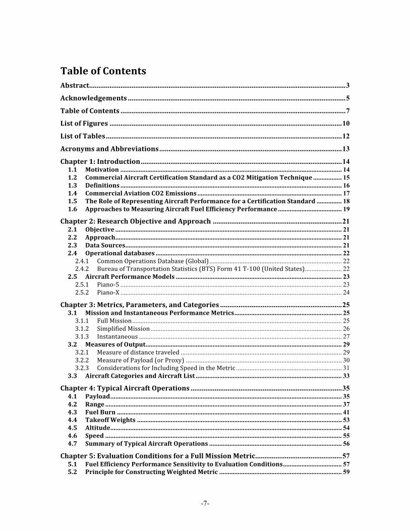
Table of Contents Abstract...........................................................................................................................................3 Acknowledgements ......................................................................................................................5 Table of Contents ..........................................................................................................................7 List of Figures ..............................................................................................................................10 List of Tables ................................................................................................................................12 Acronyms and Abbreviations ...................................................................................................13 Chapter 1: Introduction .............................................................................................................14 1.1 Motivation .................................................................................................................................... 14 1.2 Commercial Aircraft Certification Standard as a CO2 Mitigation Technique ................. 15 1.3 Definitions .................................................................................................................................... 16 1.4 Commercial Aviation CO2 Emissions ...................................................................................... 17 1.5 The Role of Representing Aircraft Performance for a Certification Standard ............... 18 1.6 Approaches to Measuring Aircraft Fuel Efficiency Performance ...................................... 19
Chapter 2: Research Objective and Approach ......................................................................21 2.1 Objective ....................................................................................................................................... 21 2.2 Approach....................................................................................................................................... 21 2.3 Data Sources................................................................................................................................. 21 2.4 Operational databases ............................................................................................................... 22 2.4.1 Common Operations Database (Global) ............................................................................... 22 2.4.2 Bureau of Transportation Statistics (BTS) Form 41 T-‐100 (United States)...................... 22
2.5 Aircraft Performance Models ................................................................................................... 23 2.5.1 Piano-‐5 .................................................................................................................................... 23 2.5.2 Piano-‐X .................................................................................................................................... 24
Chapter 3: Metrics, Parameters, and Categories ..................................................................25 3.1 Mission and Instantaneous Performance Metrics................................................................ 25 3.1.1 Full Mission............................................................................................................................. 25 3.1.2 Simplified Mission .................................................................................................................. 26 3.1.3 Instantaneous ......................................................................................................................... 27
3.2 Measures of Output..................................................................................................................... 29 3.2.1 Measure of distance traveled ................................................................................................ 29 3.2.2 Measure of Payload (or Proxy) ............................................................................................. 30 3.2.3 Considerations for Including Speed in the Metric ............................................................... 31
3.3 Aircraft Categories and Aircraft List ....................................................................................... 33 Chapter 4: Typical Aircraft Operations ..................................................................................35 4.1 Payload.......................................................................................................................................... 35 4.2 Range ............................................................................................................................................. 37 4.3 Fuel Burn ...................................................................................................................................... 41 4.4 Takeoff Weights .......................................................................................................................... 53 4.5 Altitude.......................................................................................................................................... 54 4.6 Speed ............................................................................................................................................. 55 4.7 Summary of Typical Aircraft Operations ............................................................................... 56
Chapter 5: Evaluation Conditions for a Full Mission Metric...............................................57 5.1 Fuel Efficiency Performance Sensitivity to Evaluation Conditions................................... 57 5.2 Principle for Constructing Weighted Metric ......................................................................... 59

-8-
5.3 Full Mission Metric Weighted by Range Frequency ............................................................. 60 5.4 Full Mission Metric Weighted by Fuel Burn........................................................................... 63 5.5 Issues Resulting from Evaluation Conditions Weighted based on Operational Data ... 64
Chapter 6: Evaluation Conditions for an Instantaneous Single Point Metric .................65 6.1 Atmospheric Conditions ............................................................................................................ 65 6.2 Speed and Altitude...................................................................................................................... 65 6.3 Weight ........................................................................................................................................... 68 6.4 Potential Considerations with Regard to Single Point Evaluation Schemes................... 71 6.5 Correlation with BF/R................................................................................................................ 72
Chapter 7: Case Studies - Specific Air Range and BF/R for Future Aircraft Technologies................................................................................................................................73 7.1 Case Study Vehicle: D-8.5........................................................................................................... 73 7.2 Impacts of Measurement on Future Aircraft Designs.......................................................... 75
Chapter 8: Conclusions ..............................................................................................................77 Chapter 9: Bibliography ............................................................................................................79 Chapter 10: Appendix ................................................................................................................81 10.1 Appendix A: Background Review of Aviation and Non-Aviation Certification Standards ................................................................................................................................................ 81 10.1.1 NOx ........................................................................................................................................ 81 10.1.1.1 Metric .............................................................................................................................................. 81 10.1.1.2 Correlation Parameter ................................................................................................................... 82 10.1.1.3 Evaluation Conditions.................................................................................................................... 82
10.1.2 Corporate Average Fuel Economy (CAFE) ......................................................................... 82 10.1.2.1 Metric .............................................................................................................................................. 82 10.1.2.2 Correlating Parameter ................................................................................................................... 83 10.1.2.3 Evaluation Conditions.................................................................................................................... 83 10.1.2.4 Scope of Applicability .................................................................................................................... 84
10.2 Desired Attributes of Certification Requirement .............................................................. 84 10.3 Appendix B: Aircraft List ......................................................................................................... 86

-9-
[Page Intentionally Left Blank]

-10-
List of Figures Figure 1: CO2 emissions (indexed to 2005) with targets and aspirational goals from US COP15
and IATA CO2 emissions goals and ICAO fuel efficiency goal (i.e. 2% per annum – CO2 emissions calculations assume 2005 demand). (Bonnefoy Y. M., 2011) .............................. 14
Figure 2: Notional CO2 Certification Standard .................................................................................... 15 Figure 3: Conceptual representation of aircraft level and system level inputs and outputs. ............... 17 Figure 4: Design Payload vs Design Range Across the Fleet [Data Source: Piano-X] ................... 18 Figure 5: Screenshot of Piano 5 interface (Lissys, Piano-5, 2010)................................................... 23 Figure 6: Screenshot of Piano-X interface............................................................................................. 24 Figure 7: Mission and Reserve Assumption Schematic (ICCAIA, 2010) .......................................... 26 Figure 8: Example Purchase Agreement Performance Guarantee(SEC, 1999) ............................. 27 Figure 9: Notional Payload-Range Diagram ......................................................................................... 29 Figure 10: Definition of Weight Based Parameters (Bonnefoy Y. M., 2011) .................................. 30 Figure 11: Historical Evolution of Labor Costs and Fuel Costs(Air Transport Association of
America, 2009) .................................................................................................................................. 32 Figure 12: 2006 Boeing 737-800 Operations [Data Source: BTS Form 41 T-100] ....................... 35 Figure 13: 2006 US All Carrier Payload Frequencies by Aircraft Category [Data Source: BTS
Form 41 T-100].................................................................................................................................. 36 Figure 14: 2006 Boeing 737-800 Range Frequency [Data Source: BTS Form 41 T-100] ............ 37 Figure 15: 2006 Total Fleet US All Carrier Range Frequency [Data Source: BTS Form 41 T-100]
............................................................................................................................................................... 38 Figure 16: 2006 Narrow Body Aircraft US All Carrier Range Frequency [Data Source: BTS Form
41 T-100] ............................................................................................................................................ 38 Figure 17: 2006 Wide Body Aircraft US All Carrier Range Frequency [Data Source: BTS Form
41 T-100] ............................................................................................................................................ 39 Figure 18: April 2006 Regional Jet US All Carrier Range Frequency [Data Source: BTS Form 41
T-100] .................................................................................................................................................. 40 Figure 19: 2006 Turbo Prop US All Carrier Range Frequency [Data Source: BTS Form 41 T-
100] ...................................................................................................................................................... 40 Figure 20: Piano-X Mission Simulation Grid on Notional Payload Range Chart ........................... 41 Figure 21: Bi-Cubic Fuel Burn Interpolation ........................................................................................ 42 Figure 22: 2006 US All Carrier Fleet Wide Fuel Burn, Payload Frequency, and Range Frequency
[Data Source: BTS Form 41 T-100 and Piano-X] ......................................................................... 43 Figure 23: Worldwide Fuel Burn, Payload, and Departures (Operations) by Aircraft Type [Data
Source: COD]....................................................................................................................................... 44 Figure 24: 2006 US All Carrier Wide Body Fuel Burn, Payload Frequency, and Range
Frequency [Data Source: BTS Form 41 T-100 and Piano-X]..................................................... 44 Figure 25: 2006 US All Carrier Narrow Body Fuel Burn, Payload Frequency, and Range
Frequency [Data Source: BTS Form 41 T-100 and Piano-X]..................................................... 45 Figure 26: 2006 US All Carrier Regional Jet Fuel Burn, Payload Frequency, and Range
Frequency [Data Source: BTS Form 41 T-100 and Piano-X]..................................................... 46 Figure 27: 2006 US All Carrier Regional Jet Fuel Burn, Payload Frequency, and Range
Frequency [Data Source: BTS Form 41 T-100 and Piano-X]..................................................... 47 Figure 28: April 2006 Global Operations Above and Below 1,000km by Percent Departure
(left) and Percent Fuel Burn (right) [Data Source: COD] .......................................................... 47 Figure 29: April 2006 World Wide Operations: % of Total Fuel Burned on Missions +/-
1,000km by Aircraft Type [Data Source: COD] ............................................................................ 48 Figure 30: April 2006 Percentage of Fuel Burn +/- 1,000km by Aircraft Type [Data Source:
COD] ..................................................................................................................................................... 51 Figure 31: April 2006 Cumulative Distribution of Fuel Burn, Payload, and Departures [Data
Source: COD]....................................................................................................................................... 52
-11-
Figure 32: Fuel Burn by Phase of Flight for Each Aircraft Category [Data source: COD]............. 52 Figure 33: Histogram of Useful Load at Takeoff by Aircraft Category [Data Source: BTS Form
41 T-100 and Piano-X] ..................................................................................................................... 53 Figure 34: Histogram of Aircraft Gross Weight at Takeoff by Aircraft Category [Data Source:
BTS Form 41 T-100 and Piano-X] .................................................................................................. 54 Figure 35: Actual (blue) and Ideal Flight Profile for a Boeing 757-200 from Boston to San
Francisco (Lovegren, 2011) ............................................................................................................ 55 Figure 36: BF/R vs MTOW Evaluated at Two Different Range Conditions [Data Source: Piano-X]
............................................................................................................................................................... 57 Figure 37: Margin to Regression Line [Data Source: Piano-X].......................................................... 58 Figure 38: Aircraft Ranked by Residual for Two Different Evaluation Conditions [Data Source:
Piano-X]............................................................................................................................................... 59 Figure 39: Principle for Constructing Weighted Metric..................................................................... 59 Figure 40: Fuel Efficiency Performance for Aircraft Types as a Function of R1 Range [Data
Source: PIANO-X] (Bonnefoy Y. M., 2011) .................................................................................... 60 Figure 41: Weighted Metric Normalized by Single Evaluation Condition Metric (R1) by Aircraft
Type ..................................................................................................................................................... 61 Figure 42: Comparison of Range Weighted Metric to Single Evaluation Condition Non-
Weighted Metric [Data Source: BTS Form 41 T-100 and Piano-X].......................................... 62 Figure 43: Weighted Metric Normalized by Single Evaluation Condition Metric (0.4*R1) by
Aircraft Type [Data Source: BTS Form 41 T-100 and Piano-X]................................................ 62 Figure 44: Comparison of Range Weighted Metric to Single Evaluation Condition Non-
Weighted Metric [Data Source: BTS Form 41 T-100 and Piano-X].......................................... 63 Figure 45: 1/SAR percentage changes from optimum as a function of Speed and Altitude for a
representative narrow body aircraft [Data source: PIANO-X] ................................................ 66 Figure 46: Specific Air Range Speed and Altitude Contours for a Range of Representative
Aircraft Types (Lovegren, 2011).................................................................................................... 66 Figure 47: Example 1/SAR sensitivity as a function of speed (fixed altitude and weight) for
representative aircraft for five aircraft types from the following categories: WB, NB, RJ, TP, BJ. [Data source: PIANO-X] ....................................................................................................... 67
Figure 48: Illustrative Example of Aircraft Performance Dependence on Altitude Across the Fleet [Data source: PIANO-X] .......................................................................................................... 68
Figure 49: 1/SAR and Aircraft Weight evolution over an Illustrative Mission (R1, MSP) for a Representative Narrow Body Aircraft [Data source: PIANO-X]............................................... 69
Figure 50: Takeoff Weight Iso-Contours for a Representative Narrow Body Aircraft (Boeing Airport Planning Guides) ................................................................................................................ 69
Figure 51: Aircraft weight fractions across aircraft categories [Data source: PIANO-X] ............ 70 Figure 52: Design philosophy differences: maximum structural payload and R1 range for
aircraft in five categories. [Data source: PIANO-X] .................................................................... 70 Figure 53: Notional Depiction of Aircraft Robustness to a Flight Parameter ................................ 71 Figure 54: 1/SAR vs MTOW for Piano5 Aircraft Fleet [Data Source: Piano5]................................ 72 Figure 55: Correlation of BF/R evaluated at 40% R1 with 1/SAR evaluated at (MTOW-
MZFW)/2 ............................................................................................................................................. 72 Figure 56: MIT Concept Aircraft - D8.5 .................................................................................................. 73 Figure 57: Percent Improvements in 1/SAR and BF/R for Aircraft in MIT D8.5 Morphing Study
............................................................................................................................................................... 75 Figure 58: Percent Improvements from Baseline in BF/R vs 1/SAR............................................... 75 Figure 59: NOx performance metric, correlating parameter, and regulatory levels (Bonnefoy Y.
M., 2011) ............................................................................................................................................. 81 Figure 60: Representative LTO Cycle for Aircraft Engine Certification .......................................... 82

-12-
List of Tables Table 1: Certification Status of Aircraft Weight Parameters (Bonnefoy Y. M., 2011) .................. 31 Table 2: Aircraft Categories ..................................................................................................................... 33 Table 3: Full Mission Piano-X Assumptions ......................................................................................... 42

-13-
Acronyms and Abbreviations
ACARS Aircraft Communications Addressing and Reporting System MLW Maximum Landing Weight
ANCA Airport Noise and Capacity Act MRC Maximum Range Cruise ATC Air Traffic Control MSP Maximum Structural Payload BEW Basic Empty Weight MTOW Maximum Takeoff Weight BF Block Fuel MTW Maximum Taxi Weight BJ Business Jet MVP Maximum Volumetric Payload BTS Bureau of Transportation Statistics MZFW Maximum Zero Fuel Weight
CAEP Committee on Aviation Environmental Protection NACE
National Average Carbon Emissions (Australia)
CAFE Corporate Average Fuel Economy NB Narrow Body CASFE Commercial Aircraft System Fuel Efficiency NOX Nitrous Oxides CO Carbon Monoxide OEW Operating Empty Weight CO2 Carbon Dioxide OPR Overall Pressure Ratio CP Correlation Parameter P Payload
EASA European Aviation Safety Agency PARTNER Partnership for AiR Transportation Noise and Emissions Reduction
EDS Environmental Design Space R Range
EPA Environmental Protection Agency R1 Payload-‐Range point at maximum range at MZFW
EPNdB Effective Perceived Noise Level, in decibels R2 Payload-‐Range point at intersection of MTOW and maximum fuel volume
FAA Federal Aviation Administration RJ Regional Jet FL Floor Area SA Single Aisle GHG Greenhouse Gas SAR Specific Air Range
GIACC Group on International Aviation and Climate Change SEW Standard Empty Weight
GVWR Gross Vehicle Weight Rating SOX Sulfurous Oxides H20 Water STA Small Twin Aisle HC Hydro Carbon SUV Sport Utility Vehicle ICAO International Civil Aviation Organization TCDS Type Certificate Data Sheet ISA International Standard Atmosphere TOGW Takeoff Gross Weight L/D Lift to Drag ratio TP Turboprop LQ Large Quad TSFC Thrust Specific Fuel Consumption LRC Long Range Cruise UL Useful Load
LTA Large Twin Aisle UNFCCC United Nations Framework Convention on Climate Change
LTO Landing and Take-‐Off WB Wide Body MEW Manufacturer Empty Weight WG3 (ICAO CAEP) Working Group 3
-14-
Chapter 1: Introduction
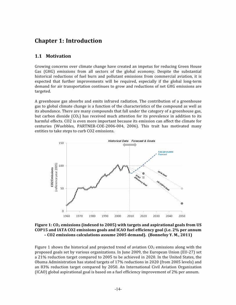
1.1 Motivation Growing concerns over climate change have created an impetus for reducing Green House Gas (GHG) emissions from all sectors of the global economy. Despite the substantial historical reductions of fuel burn and pollutant emissions from commercial aviation, it is expected that further improvements will be required, especially if the global long-‐term demand for air transportation continues to grow and reductions of net GHG emissions are targeted. A greenhouse gas absorbs and emits infrared radiation. The contribution of a greenhouse gas to global climate change is a function of the characteristics of the compound as well as its abundance. There are many compounds that fall under the category of a greenhouse gas, but carbon dioxide (CO2) has received much attention for its prevalence in addition to its harmful effects. CO2 is even more important because its emission can affect the climate for centuries (Wuebbles, PARTNER-‐COE-‐2006-‐004, 2006). This trait has motivated many entities to take steps to curb CO2 emissions.
Figure 1: CO2 emissions (indexed to 2005) with targets and aspirational goals from US COP15 and IATA CO2 emissions goals and ICAO fuel efficiency goal (i.e. 2% per annum
– CO2 emissions calculations assume 2005 demand). (Bonnefoy Y. M., 2011)
Figure 1 shows the historical and projected trend of aviation CO2 emissions along with the proposed goals set by various organizations. In June 2009, the European Union (EU-‐27) set a 21% reduction target compared to 2005 to be achieved in 2020. In the United States, the Obama Administration has stated targets of 17% reductions in 2020 (from 2005 levels) and an 83% reduction target compared by 2050. An International Civil Aviation Organization (ICAO) global aspirational goal is based on a fuel efficiency improvement of 2% per annum.
-15-
While commercial aviation contributed approximately 2.5% of total anthropogenic CO2 emissions in 2005 (Lee, 2009), aviation’s relative contribution to climate change is estimated to be higher (Solomon, 2007), due in part to the types of emissions produced and the high altitude at which the majority of emissions are produced. Aviation’s relative contribution to climate change is only expected to grow, as other sectors mitigate their emissions production while demand for aviation continues to increase. The identification of CO2 as a leading contributor to climate change, coupled with concern over the potentially increasing contribution of CO2 emissions to climate change by aviation, motivates action to assess measures to mitigate aviation’s CO2 emissions in the near-‐term.
1.2 Commercial Aircraft Certification Standard as a CO2 Mitigation Technique
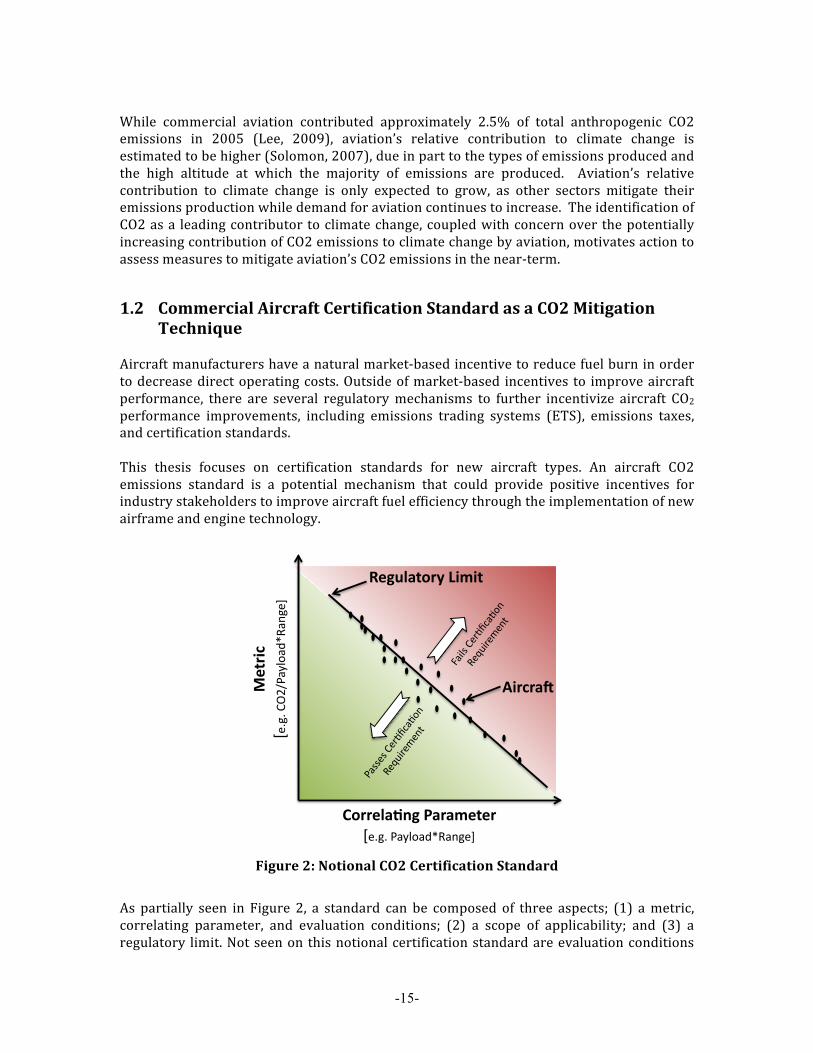
Aircraft manufacturers have a natural market-‐based incentive to reduce fuel burn in order to decrease direct operating costs. Outside of market-‐based incentives to improve aircraft performance, there are several regulatory mechanisms to further incentivize aircraft CO2 performance improvements, including emissions trading systems (ETS), emissions taxes, and certification standards. This thesis focuses on certification standards for new aircraft types. An aircraft CO2 emissions standard is a potential mechanism that could provide positive incentives for industry stakeholders to improve aircraft fuel efficiency through the implementation of new airframe and engine technology.
Figure 2: Notional CO2 Certification Standard
As partially seen in Figure 2, a standard can be composed of three aspects; (1) a metric, correlating parameter, and evaluation conditions; (2) a scope of applicability; and (3) a regulatory limit. Not seen on this notional certification standard are evaluation conditions
!"#$%&'
!"#$#%&'()*+,-.+/0
1+2$"3%
()$$"*+,-.'/+$+0"#"$'!"#$#%*+,-.+/01+2$"3%
1%$&$+2'
3".4*+#)$5'6%0%#'
4+5-6%&"789:+8.2%%
1";<57"="2>%
*+66"6%&"789:+8.2%%
1";<57"="2>%
-16-
and scope of applicability. Evaluation conditions refer to the conditions at which the metric and correlating parameter are measured to demonstrate compliance, and scope of applicability refers to the types of aircraft that must show compliance with the standard. A correlating parameter is not a necessary part of the standard (e.g. can consist only of a metric and a regulatory level). However, in some cases it might be appropriate for the standard to vary with as a function of a vehicle attribute, such as size. In this case, a regulatory level can be defined as a function of the correlating parameter. A technology forcing standard applies pressure to manufacturers to develop new technology while a technology following standard sets the limit such that all new aircraft must meet the best technology available. The position of the regulatory level determines if the standard is technology forcing or technology following. Currently ICAO, a United Nations (UN) committee, is undertaking a consensus-‐based attempt to establish a CO2 certification standard that is developed with the technical input and commitment from all member states, regulatory agencies, industry representatives, and special interests. This attempt limits the scope of applicability to new aircraft types (i.e. not used to force aircraft retirement in the existing fleet). The scope of applicability includes new jet aircraft types with a maximum takeoff weight (MTOW) above 5700kg and new turboprop aircraft types with a MTOW above 8618kg. The CO2 Task Group (CO2TG) within ICAO is tasked with developing recommendations for the metric, correlating parameter, and evaluation conditions.
1.3 Definitions1 Metric: The metric generally captures the performance parameter that is to be influenced (i.e. Fuel Burn or CO2). Plotted on the y-‐axis of graphs Correlating Parameter (CP): Based on fundamental vehicle attributes (e.g. size). Correlating parameters reflect fundamental physical tradeoffs between vehicle capability and the performance parameter that is to be influenced. Evaluation Condition: Condition at which the vehicle performance is measured and reported to show compliance. These measurement conditions are intended to be representative of actual conditions, but may not precisely predict actual vehicle in day-‐to-‐day operations. Regulatory Level: sets the performance goals (y-‐axis) to be achieved for a product with a given capability (x-‐axis). This regulatory level function generally captures the physics based relationship between the metric and the CP. Subsequent regulatory levels are generally set by sliding down.
1 Bonnefoy, Y. M. (2011). Assessment of CO2 Emission Metrics for a Commercial Aircraft Certification Requirement. PARTNER.
-17-
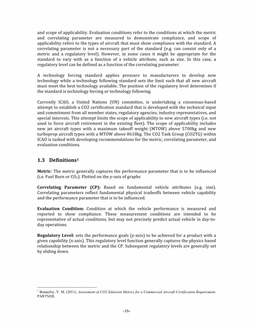
1.4 Commercial Aviation CO2 Emissions Figure 3 shows a schematic representation of aircraft and system input and output. Each aircraft in the National Airspace System (NAS) uses fuel to deliver air transportation output (movement of persons or cargo) while producing emissions (CO2, H2O, NOx, PM, etc).
From first principles, total fleet-‐wide CO2 emissions from commercial aviation are function of three key factors:
(1) Fuel CO2 content (2) Aircraft Fuel Efficiency (3) Operational factors
Item (1) is defined as the amount of CO2 released per extracted unit of energy from the fuel. Item (2) is defined as the amount of productivity delivered by the aircraft during the use of a unit of fuel energy. The operational factors in (3) are composed of mass load factors less than 100%, air traffic control system inefficiencies, and airline inefficiencies. The product of these factors is summed over the total actual air transportation output, as seen in Equation 1 in order to arrive at total fleet-‐wide CO2 emissions.
€
CO2Emissions =CO2
Fuel_ Energy⎛
⎝ ⎜
⎞
⎠ ⎟
Output∑ * Fuel_ Energy
Output⎛
⎝ ⎜
⎞
⎠ ⎟ *
1ηLFηATCηAirlines
⎛
⎝ ⎜
⎞
⎠ ⎟ Equation 1
The second term of this equation is the aircraft level performance measure of interest to this research.
€
Metric =Fuel_ Energy
Output Equation 2
The metric can easily be transformed into CO2/Output by multiplying Equation 2 by the Fuel CO2 Content for a reference fuel. The reason for decomposing the metric in this way is to isolate aircraft performance improvements or degradations from those of the fuel.
Figure 3: Conceptual representation of aircraft level and system level inputs and outputs.

-18-
1.5 The Role of Representing Aircraft Performance for a Certification Standard
Airplanes must operate safely and efficiently within a complex environment of physical and regulatory constraints. In addition, the manufacturer must meet a wide variety of customer needs with a desirable product while returning a reasonable amount of profit to the company in order to sustain production (ICCAIA, 2010). The range of aircraft sizes under the scope of a certification standard is board and encompasses short-‐range turbo props to low-‐payload, long-‐range business jets to wide body transport aircraft like the Airbus A380 with 500+ seats, as seen in Figure 4.
Figure 4: Design Payload vs Design Range Across the Fleet [Data Source: Piano-X]
Moreover, aircraft consume vastly different amounts of fuel to fly their design missions. This result is due partly to the fact that aircraft are designed with different levels of technology, but mostly because of the inherent differences between aircraft with differing design specifications intended to serve different market needs. One way to attempt to reconcile this difference is to include some measure of “productivity” to attempt to account for variations across the fleet. This can be in the form of range, a measure of “what is transported” (i.e. payload or a payload proxy), or speed. Aircraft are also designed with an ability to fly a diversity of missions partly due to operator network demands and to provide flexibility for potential multiple owners throughout the aircraft’s service lifetime. Fuel efficiency performance encompasses a wide range of aircraft capabilities. While much of the marketing focus and available published data is usually concerned with peak performance, most operations do not normally take place at these maximum points. It is the enormous operational flexibility of most aircraft that make them suited for a host of off-‐
!"
#!$!!!"
%!$!!!"
&!$!!!"
'!$!!!"
(!$!!!"
)!$!!!"
*!$!!!"
+!$!!!"
,!$!!!"
!" %$!!!" '$!!!" )$!!!" +$!!!" #!$!!!" #%$!!!" #'$!!!" #)$!!!"
!"#$%
&%'()*&+)&*",'-".,/"0
'1234'
56'5"738'12%4'
!"#$%
&'"'(#$$%)*+$%
,-.%/$$%
&'''(0$$1-%
!2-(30% !"#$%&'()&%"'*+,-.'/'(0'1234'
!"#$%&'*).5,)
6'*+,-.'/'78*'12
%4'
!"
#!$!!!"
%!$!!!"
&!$!!!"
'!$!!!"
(!$!!!"
)!$!!!"
*!$!!!"
+!$!!!"
,!$!!!"
!" %$!!!" '$!!!" )$!!!" +$!!!" #!$!!!"#%$!!!"#'$!!!"#)$!!!"
!"#$%
&%'()*&+)&*",'-".,/"0
'1234'
56'5"738'12%4'
-./0"12/3"
456627"12/3"
809.2:5;"<0="
>?6@2"A62B"
1?C.:0CC"<0="

-19-
design missions. At the same time, the performance figures realized at one condition may not apply at another (ICCAIA, 2010). Due to this diversity of operations, even if an appropriate metric were available, there is no obvious evaluation point a priori with regard to payload, range, speed, altitude, etc.
1.6 Approaches to Measuring Aircraft Fuel Efficiency Performance Conventionally, performance measures, the most popular of which is the Corporate Average Fuel Efficiency (CAFE) standard for US automobiles, are mission based. That is, fuel burn (or emissions) are summed over the course of an assumed mission designed to represent typical operations. Defining block fuel (or mission fuel) for the basis of an aircraft level manufacturer certification standard is quite complicated. A manufacturer study identified over 150 assumptions and parameter definitions required to fully define a mission for a simulation tool (ICCAIA, 2010). This greatly complicates the certification procedure and adds even more burden to defining a representative measure of aircraft performance. There may be an opportunity to greatly simplify certification burden and complexity by using a single, instantaneous measurement that still reflects aircraft performance on a diversity of typical aircraft operations. Specific Air Range (SAR) is a traditional measure of aircraft cruise performance which measures the distance an aircraft can travel for a unit of fuel mass.
€
SAR =dR
−dWf
=V
Fuel Flowmeasured in km
kg Equation 3
SAR is analogous to ‘miles-‐per-‐gallon’ for automobiles, except instead of integrating the measurement over a full reference mission, the measurement would be taken at a single representative point (e.g. 55mph, 2 passengers, 50% fuel, auxiliary power off). This thesis attempts to determine how to define evaluation conditions for mission-‐based and instantaneous metrics. SAR is also evaluated against BF/R for potential future technologies to determine if a single point instantaneous measure of aircraft performance is a reasonable certification standard surrogate for a more detailed but cumbersome mission-‐based measurement.


Chapter 2: Research Objective and Approach
2.1 Objective The objective of this research is to:
1) Assess typical commercial aircraft operations in order to inform the evaluation of mission and instantaneous performance metrics.
2) Define representative evaluation conditions for mission-‐based metrics. 3) Define representative evaluation conditions for instantaneous point metrics. 4) Determine if an instantaneous point metric could be a reasonable surrogate
for mission fuel metric despite its inherent simplicity, and identify any differences.
The end result of this effort is a potential evaluation condition for mission and instantaneous point metrics based on typical aircraft operations, an assessment of the correlation between the two metrics at their evaluation conditions, and an assessment of mission and instantaneous metric correlation for future aircraft designs.
2.2 Approach First, a list metrics and correlating parameters were defined. Operational data was then used to assess typical aircraft operations in order to inform the evaluation of mission and instantaneous performance metrics. Mission metrics were weighted by operation parameters to determine if a representative single evaluation condition sufficiently represents typical aircraft operations. Assumptions required to define instantaneous point metric evaluation conditions were made based on first principles and typical aircraft operations. Finally, a future aircraft design was evaluated to determine if the instantaneous point metric improvements correlate with mission metric improvements.
2.3 Data Sources Several analysis tools and data sources were used in the evaluation of current fleet performance. The assumptions, fields, and aggregation techniques inherent to each source are important to understanding any result limitations.

2.4 Operational databases
2.4.1 Common Operations Database (Global) The Common Operations Database (COD)2 is a global flight-‐by-‐flight operational database. Each line in the database represents a single aircraft flight and contains aircraft identifiers (aircraft type, engine type); origin/destination information (airport, country); and payload, range, and fuel burn by phase of flight.3 The COD is constructed from Eurocontrol's (EC) Enhanced Traffic Flight Management System (ETFMS), FAA's Enhanced Traffic Management System (ETMS), and International Official Airline Guide (IOAG) data. ETFMS and ETMS account for up to ~75% of global commercial operations, while ETMS alone covers ~55%, and the remainder of worldwide operations are covered by IOAG year 2006 schedule. Payload is not directly reported on a flight-‐by-‐flight basis, therefore assumptions were used to calculate payload in the COD. Equation 4 describes the assumptions used to populate the COD payload data. Passenger payload is computed by multiplying the passenger payload factor by the number of seats and average passenger weight. Cargo payload is computed by multiplying the cargo load factor by the available cargo capacity. Specifically, I or D specifies international or domestic; Wp is the average passenger weight (91kg); PLF is the passenger load factor; CLF(BEL) is the cargo load factor on passenger flights; and CLF(FRT) is the cargo load factor on freight flights.
Equation 4
For a specific aircraft type, Wp, median seats, and median max structural payload are constant. PLF and CLF vary by region and category (I or D). Because there are 6 regions, 2 categories, and 2 load factors (PLF and CLF), payload is aggregated into 24 bins for each aircraft (MODTF Rapporteurs, 2008).
2.4.2 Bureau of Transportation Statistics (BTS) Form 41 T-100 (United States) Because of the high level of payload aggregation in the COD, a second operational database was obtained, but is limited to United States operations. The Bureau of Transportation Statistics (BTS) Form 41 Schedule T-‐100 U.S. all-‐carrier (international and domestic)
2 International Civil Aviation Organization, Committee on Aviation Environmental Protection, Modelling and Databases Group’s 2006 Common Operations Database; Jointly maintained by U.S.DOT’s Volpe Center, on behalf of the Federal Aviation Administration, and EUROCONTROL’s Experimental Center; CAEP/9 Version. 3 Columns: DATE; DEP_APT_CODE; ARR_APT_CODE; DEP_CNTRY_CODE; ARR_CNTRY_CODE; AIRCRAFT_TYPE; ENGINE_TYPE; AIRCRAFT_ROLE; TRAJECTORY_TYPE; DEP_BELOW10K_DISTANCE; ABOVE10K_DISTANCE; ARR_BELOW10K_DISTANCE; TOTAL_DISTANCE; DEP_BELOW10K_FUELBURN; ABOVE10K_FUELBURN; ARR_BELOW10K_FUELBURN; TOTAL_FUELBURN; PAYLOAD; SEATS_MEDIAN; OEW_MEDIAN; MTOW_MEDIAN; FUEL_CAPACITY_MEDIAN; MSP_MEDIAN
!
PayloadI /D (PAX) = [PLFI /D *Median _ Seats*WP ]+ [CLF(BEL)I /D * (Median _Max _ Structure_Payload "Median _ Seats*WP )]
!
PayloadI /D (Cargo) = CLF(FRT)I /D *Median _Max _ Structure_Payload

-23-
segment data for the full year 20064 provided base year operational data. Data was filtered to exclude cargo service, military flights, repositioning flights (i.e. departures performed with zero passengers reported), and sightseeing (i.e. departures performed whose origin and destination were the same airport). Each entry in the database is a monthly aggregation of a unique aircraft type, operator, and origin-‐destination (OD) pair.
2.5 Aircraft Performance Models
2.5.1 Piano-5 Piano-‐5 is an integrated tool for analyzing and comparing existing or projected commercial aircraft. It consists of a 250+ aircraft database, a flight simulation module, and an aircraft redesign tool. Piano's aircraft database (Appendix B: Aircraft List) contains existing types as well as projected developments. Each aircraft has been calibrated according to the best data available from both private and public sources. Piano's models are constructed independently on the basis of generally available, non-‐confidential information and descriptions, and are not in any way endorsed by the manufacturers or by any other organization (Lissys, Piano-‐5, 2010).
Figure 5: Screenshot of Piano 5 interface (Lissys, Piano-5, 2010)
Piano 5 allows realistic manipulation of most design parameters (Figure 5) by redesigning the aircraft using user specified criteria. For example, the user could opt to re-‐engine the aircraft with an updated TSFC and no change to the airframe, or the user could update engine TSFC and reoptimize the aircraft (i.e. design a new aircraft) for the same or a new mission. This capability will allow realistic evaluation of performance metrics under the influence of new technology. While Piano’s models and redesign capabilities have not been validated by any manufacturer, it is the best available secondary data source. 4 http://www.transtats.bts.gov/DL_SelectFields.asp?Table_ID=309&DB_Short_Name=Air%20Carriers

-24-
2.5.2 Piano-X Piano-‐X is similar to Piano 5 without the aircraft redesign tool. Piano-‐X contains an aircraft database (Appendix B: Aircraft List) and flight simulation module.
Figure 6: Screenshot of Piano-X interface
Piano-‐X allows the input of speed preference, altitude constraints, reserve, diversion, and taxi in/out times in order to provide a realistic simulation. Multiple output formats are possible, including block fuel summaries (fuel, time, CO2, NOx, etc) and detailed flight profiles (time, altitude, and fuel burn at steps along the mission).

Chapter 3: Metrics, Parameters, and Categories There are two approaches to quantifying aircraft fuel efficiency performance: (1) full mission metrics and (2) instantaneous metrics. Full mission metrics encompass all flight phases and require a large set of assumptions to define in the context of a certification standard. A subset of the full mission approach is to simplify measurements by excluding certain phases of flight. The instantaneous approach can either measure fuel efficiency performance at one point or multiple points. Using the form identified in Equation 2, fuel efficiency metrics are defined as Fuel_Energy/Output. Any measure of transportation output must include some measure of distance traveled. Therefore, for the purpose of this research, output is defined as range. Because there is no mathematical difference between defining an output term in the denominator of the metric or on the correlating parameter, other forms of output (e.g. payload or payload proxy) are included in the correlating parameter. In this chapter, full mission and instantaneous fuel efficiency metrics are defined. In addition, range parameters, and payload proxies are detailed. Speed is examined for inclusion in a metric or CP, and a list of aircraft and categories are presented.
3.1 Mission and Instantaneous Performance Metrics
3.1.1 Full Mission The performance of the aircraft is measured for the entire mission. The full mission (FM) metric is defined in Equation 5 as Block Fuel divided by mission range.
€
FM =Block _FuelRange
Equation 5
Block fuel measurement starts as the aircraft moves from the departure gate and stops at the arrival gate. Figure 7 shows a typical mission and reserve schematic. As can be seen in this figure, block fuel encompasses all flight phases from taxi-‐out to taxi-‐in.

-26-
Figure 7: Mission and Reserve Assumption Schematic (ICCAIA, 2010)
Full mission definition requires many assumptions with regard to payload, range, climb schedules, etc. A single phase of the block fuel mission contains many sub-‐phases. For example, taxi consists of start-‐up, engine warm-‐up, overcoming stiction, acceleration to taxi speeds, turns, stops, and re-‐starts (ICCAIA, Sept 2010). Each taxi phase varies by ground congestion and airport geography (weather and terrain). Calculation of block fuel also requires the definition of reserves (Figure 7), which typically vary by operator and crew. While reserve fuel is not counted as “fuel burned” during the calculation of block fuel, it is important to include due to the extra weight carried during the mission. Reserve fuel is defined by operational requirements (FAR121 or EU-‐OPS 1.255) and is mandated to cope with deviations between predicted flight plan and actual flight. By it’s nature, block fuel is driven heavily by operational constraints (noise on takeoff, taxi times, mission rules by OD pair, overwater routes, etc). While block fuel is predictable based on manufacturer models, its accuracy is a function of the appropriate operational assumptions of how the aircraft will be flown (ICCAIA, Sept 2010). To be used in a certification standard, these assumptions would need to be fully defined.
3.1.2 Simplified Mission Simplified missions are a subset of full missions, and exclude some phases of flight. For example, in Figure 7 “Still Air Range” is a simplified mission because it excludes the taxi, takeoff, approach, and land phases. Simplified mission measurements attempt to limit the number of assumptions required to define the evaluation condition for the certification requirement. Simplified mission metrics also attempt to limit the influence of operationally driven phases of flight.
CAEP9_WG3_CO2-2_WPXX
Page 2 of 11
200 nmi
Clim
b
Cruise* @ LRC
App
roac
h an
d la
nd
30 M
in. h
old
@ 1
,500
ft
Mission ReservesDefined by operational rule jurisdiction
e.g. FAR International Mission Rules
Still air rangeFlight time & fuelBlock time & fuel
Numerous assumptions/definitions required to sufficiently describe a “mission” for the purposes of calculating performance:Aircraft definition, performance level, payload level, route (or distance) definition, airport definition, operational rule jurisdiction, operational techniques, environmental factors, fuel quality, etc.
Fig 1. Mission Profile Descriptor – illustration of the mission elements typically used for the calculation of aircraft performance (fuel burn, payload capability, range capability)
Acc
eler
ate
to c
limb
spee
d
Clim
b to
10,
000
ft a
t 250
kts
Clim
bout
and
acce
lera
teto
1,5
00 f
t & 2
50kt
s
Taxi
out
(xx
min
.)
Take
off
to 3
5 ft
Clim
b
Des
cend
and
dec
eler
ate
to 1
0,00
0 ft
and
250
kts
App
roac
h an
d la
nd
Taxi
in (y
ym
in. f
rom
res
erve
s)
Fuel
for
10%
flig
ht t
ime
@
LRC
Mac
h, f
inal
alt.
and
wt.
Mis
sed
appr
oach
Des
cend
Des
cend
to 1
,500
ft a
t 250
kts
Mission Profile & Fuel Requirements Descriptor
Cruise (w/Steps)
* e.g. defined as >zz% of Alternate Distance
-27-
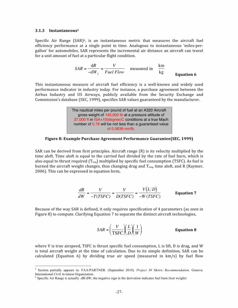
3.1.3 Instantaneous5 Specific Air Range (SAR)6, is an instantaneous metric that measures the aircraft fuel efficiency performance at a single point in time. Analogous to instantaneous ‘miles-‐per-‐gallon’ for automobiles, SAR represents the incremental air distance an aircraft can travel for a unit amount of fuel at a particular flight condition.
Equation 6 This instantaneous measure of aircraft fuel efficiency is a well-‐known and widely used performance indicator in industry today. For instance, a purchase agreement between the Airbus Industry and US Airways, publicly available from the Security Exchange and Commission’s database (SEC, 1999), specifies SAR values guaranteed by the manufacturer.
Figure 8: Example Purchase Agreement Performance Guarantee(SEC, 1999)
SAR can be derived from first principles. Aircraft range (R) is its velocity multiplied by the time aloft. Time aloft is equal to the carried fuel divided by the rate of fuel burn, which is also equal to thrust required (Treq) multiplied by specific fuel consumption (TSFC). As fuel is burned the aircraft weight changes, thus changing drag and Treq, time aloft, and R (Raymer, 2006). This can be expressed in equation form,
€
dRdW
=V
−T(TSFC)=
VD(TSFC)
=V L D( )
−W (TSFC) Equation 7
Because of the way SAR is defined, it only requires specification of 4 parameters (as seen in Figure 8) to compute. Clarifying Equation 7 to separate the distinct aircraft technologies,
€
SAR =V
TSFC⎛
⎝ ⎜
⎞
⎠ ⎟ LD⎛
⎝ ⎜
⎞
⎠ ⎟ 1W⎛
⎝ ⎜
⎞
⎠ ⎟ Equation 8
where V is true airspeed, TSFC is thrust specific fuel consumption, L is lift, D is drag, and W is total aircraft weight at the time of calculation. Due to its simple definition, SAR can be calculated (Equation 6) by dividing true air speed (measured in km/s) by fuel flow
5 Section partially appears in: FAA/PARTNER. (September 2010). Project 30 Metric Recommendation. Geneva: International Civil Aviation Organization. 6 Specific Air Range is actually -dR/dW; the negative sign in the derivation indicates fuel burn (lost weight)
!
SAR =dR
"dWf
=V
Fuel Flowmeasured in km
kg!
The nautical miles per pound of fuel at an A320 Aircraft gross weight of 145,000 lb at a pressure altitude of
37,000 ft in ISA+10(degree)C conditions at a true Mach number of 0.78 will be not less than a guaranteed value
of 0.0839 nm/lb. !

-28-
(measured in kg/s). L/D and, to a lesser extent, TSFC are functions of altitude and atmospheric conditions. Thus, when measured in steady-‐level conditions, SAR depends only on aircraft weight, altitude, air speed, ambient temperature and some operational assumptions such as electrical power extraction, operation of the air conditioning system, and aircraft center of gravity location in terms of the mean aerodynamic chord. This makes SAR relatively simple in comparison to full-‐mission metrics in 3.1.1 Full Mission. In addition, SAR encapsulates fundamental parameters that directly influence airplane fuel efficiency including: propulsion system efficiency (V/TSFC), aerodynamic efficiency (L/D), and airplane weight (1/W). The first term (V/TSFC) of Equation 8 is equivalent to (T*V)/(Fuel Flow*Heating Value) for a given fuel type, which denotes the ratio of the time rate of work done to the time rate of chemical energy input, also known as the overall efficiency of a propulsion system. The second term (L/D) of Equation 8 is the lift-‐to-‐drag ratio, a well-‐known parameter that represents aerodynamic efficiency of an airplane. The last term is airplane weight at the evaluation condition, which includes airframe weight. Therefore, SAR is able to capture the progression of CO2 reduction technologies encompassing the areas of aerodynamics, propulsion system, and airframe weight reduction. While these fundamental parameters are included in Equation 8, the equivalent definition of SAR as V / Fuel Flow (Equation 6) is anticipated to allow the evaluation of SAR either by demonstration through flight tests or numeric analysis. Numerical analysis is typically done using an airplane performance model calibrated and validated through analyses and flight tests. Although not required by airworthiness authorities, manufacturers conduct a number of flight tests during the certification process to validate cruise performance for the development of flight manuals that are supplied to the operators. Due to this common use, it is expected that SAR would be relatively easy to certify compared to mission-‐based metrics, which require numerous parameters to be defined and agreed upon, by a regulatory authority as well as complex methodology to implement within the certification process. Although SAR is a point-‐based metric measured for a single aircraft, the fleet fuel burn performance communicated to the public could be calculated based on certification data. Although SAR is widely used in the aeronautical engineering community, the reciprocal of SAR (1/SAR) is used in this research for two reasons. First, there is a general consensus amongst regulatory bodies that a CO2 metric should be in a form of CO2 emissions normalized by a parameter or a product of parameters. The reciprocal of SAR represents the amount of fuel required per a unit air distance, and thus is consistent with this general metric form (i.e. fuel burn per unit of air transportation output). Secondly, by using 1/SAR along with the appropriate CP, a reduction in the metric indicates an improvement, which is consistent with the nature of mission-‐based metrics. This consistent principle metric form facilitates the common assessment of 1/SAR and block fuel metrics, since both can be investigated for improvement trends in the same direction.

3.2 Measures of Output A major consideration in the definition of candidate fuel efficiency metrics is how to define “Output” in Equation 1. The purpose of air transportation is to transport people and goods over some distance in some amount of time. Thus, air transportation output can be constructed using one or a combination of the following high-‐level parameters:
(1) Measure of distance traveled (2) Measure (or proxy) of what is transported (3) Measure of speed (or time)
3.2.1 Measure of distance traveled Any measure of transportation productivity must include some measure of distance traveled. There are two ways to reference distance: first, absolute distance in terms of miles or kilometers; or second, a relative distance that is defined as a fraction of some measure of aircraft range capability.
Figure 9: Notional Payload-Range Diagram
Figure 9 depicts a notional payload-‐range diagram. The boundary of the diagram is limited by characteristics of the aircraft (e.g. Maximum Structural Payload (MSP), max landing weight, MTOW, and fuel capacity). The region inside of the boundary represents feasible combinations of payload and range (missions). A contour inside of the boundary and parallel with the MTOW limited boundary represents lines of constant takeoff weight (TOW) (i.e. all combinations of payload and range on a given line can be achieved by a single TOW). In order to achieve a different mission at the same TOW, the proportion of payload and fuel must be changed.
!"#!"$#
!%#
!"#$%&'()&('"*$+",*-".$/010$!234$5/6/&1.$$
!"#$5"7./78$41/89&$5/6/&1.$
!"#/6(6$:";1-<$$41/89&$5/6/&1.$
3(1*$=">")/&,$$5/6/&1.$
?"781$
+",*-"
.$
&'()*#+,#-+(*.$(.##/$0)+1#2)'34.#
-30-
R1 is a commonly used reference distance. It is the intersection of the MSP limited line and the MTOW (or max landing weight) limited line. R1 represents the maximum range an aircraft can fly the MSP. For this reason, R1 serves in this research as a proxy for aircraft design range. R1a is depicted here for completeness. Not all aircraft are max landing weight limited on their payload-‐range boundary as this only happens when the reserve fuel for long-‐range missions is very large. In this research, relative distance measurements are preferred over absolute distance measurements due to design differences inherent to the aircraft fleet. There is a factor of 15 difference between the shortest and longest R1 range amongst aircraft in this study (Piano-‐X). Thus, fractions of R1 range are used, as it is convenient to compare aircraft on a similar relative basis.
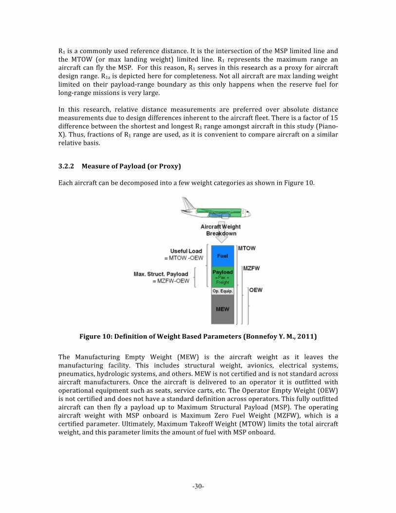
3.2.2 Measure of Payload (or Proxy) Each aircraft can be decomposed into a few weight categories as shown in Figure 10.
Figure 10: Definition of Weight Based Parameters (Bonnefoy Y. M., 2011)
The Manufacturing Empty Weight (MEW) is the aircraft weight as it leaves the manufacturing facility. This includes structural weight, avionics, electrical systems, pneumatics, hydrologic systems, and others. MEW is not certified and is not standard across aircraft manufacturers. Once the aircraft is delivered to an operator it is outfitted with operational equipment such as seats, service carts, etc. The Operator Empty Weight (OEW) is not certified and does not have a standard definition across operators. This fully outfitted aircraft can then fly a payload up to Maximum Structural Payload (MSP). The operating aircraft weight with MSP onboard is Maximum Zero Fuel Weight (MZFW), which is a certified parameter. Ultimately, Maximum Takeoff Weight (MTOW) limits the total aircraft weight, and this parameter limits the amount of fuel with MSP onboard.

Table 1: Certification Status of Aircraft Weight Parameters (Bonnefoy Y. M., 2011)
Availability of Certified Metrics Acronym Metric
Aircraft Manufacturer Certification Operator Certification
MTW Maximum taxi weight Certified N/A
MTOW Maximum takeoff weight Certified N/A
MLW Maximum landing weight Certified N/A
MZFW Maximum zero fuel weight Certified N/A
OEW Operating empty weight Not Certified Certified (in Airplane Flight Manual)
Max. Payload Maximum Payload Not Certified Certified (in Airplane Flight Manual)
MEW Manufacturer’s empty weight Not Certified N/A
While some weight parameters are not certified (Table 1) at the manufacturer stage, they are certified by the operator in the aircraft flight manual in order to inform pilots during flight planning. Parameters that are not certified by the manufacturer do not have consistent definitions across manufacturers or operators. There is no certified payload parameter. The definition of MSP is MZFW-‐OEW, which is not certified as OEW varies across manufacturers and operators. Other measures of ‘What is Transported’ include floor area, volume, number of seats, or some combination of these. Floor area was eliminated from consideration due to the lack of a standard definition across manufacturers and the potential gaming of a standard based on floor area (i.e. increases in “non-‐productive” floor area in order to beat the standard). Volume was eliminated from consideration for this same reason. Number of seats is a highly dependant on operational considerations. For example, a B737-‐700 can be outfitted with a standard ~126-‐seat configuration, or it can be outfitted with an all business class configuration. The manufacturer has no control over the number of seats that are outfitted by the operator; thus, in this example there is a large difference between the certification value of the metric and the “day-‐to-‐day” value of the metric. For these reasons, the parameters of interest to this research are MTOW, MZFW, and OEW (while not certified, is the only available parameter to be used as a proxy to calculate payload).
3.2.3 Considerations for Including Speed in the Metric There are consequences for including speed in a proposed metric, and there are potential implications for not including any measure of speed. First, Block Fuel and Speed are coupled at the operational level and design level. The cruise speed at which airlines choose to fly the aircraft (operational) influences fuel burn. From a design stand point, aircraft
-32-
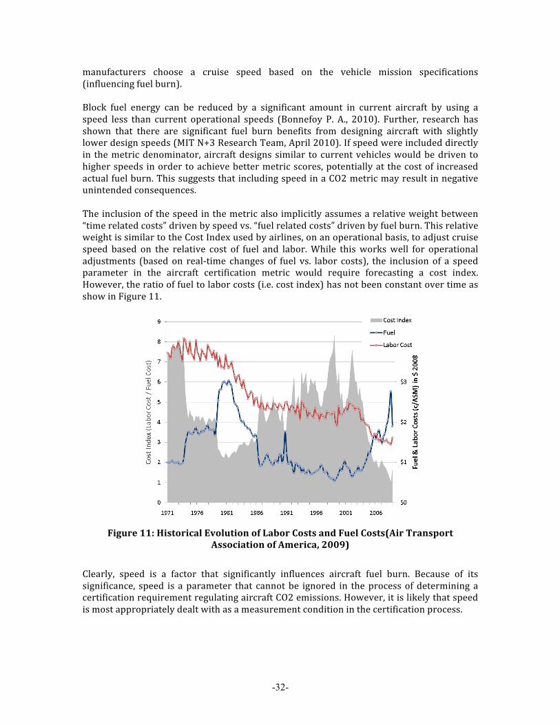
manufacturers choose a cruise speed based on the vehicle mission specifications (influencing fuel burn). Block fuel energy can be reduced by a significant amount in current aircraft by using a speed less than current operational speeds (Bonnefoy P. A., 2010). Further, research has shown that there are significant fuel burn benefits from designing aircraft with slightly lower design speeds (MIT N+3 Research Team, April 2010). If speed were included directly in the metric denominator, aircraft designs similar to current vehicles would be driven to higher speeds in order to achieve better metric scores, potentially at the cost of increased actual fuel burn. This suggests that including speed in a CO2 metric may result in negative unintended consequences. The inclusion of the speed in the metric also implicitly assumes a relative weight between “time related costs” driven by speed vs. “fuel related costs” driven by fuel burn. This relative weight is similar to the Cost Index used by airlines, on an operational basis, to adjust cruise speed based on the relative cost of fuel and labor. While this works well for operational adjustments (based on real-‐time changes of fuel vs. labor costs), the inclusion of a speed parameter in the aircraft certification metric would require forecasting a cost index. However, the ratio of fuel to labor costs (i.e. cost index) has not been constant over time as show in Figure 11.
Figure 11: Historical Evolution of Labor Costs and Fuel Costs(Air Transport
Association of America, 2009)
Clearly, speed is a factor that significantly influences aircraft fuel burn. Because of its significance, speed is a parameter that cannot be ignored in the process of determining a certification requirement regulating aircraft CO2 emissions. However, it is likely that speed is most appropriately dealt with as a measurement condition in the certification process.

-33-
3.3 Aircraft Categories and Aircraft List An objective of this research is to identify performance for a wide variety of aircraft. Aircraft in this study span sizes from 4,500kg to 600,000kg and 6 seats to 800 seats. An aircraft list is included in Appendix B: Aircraft List. Broad classification schemes were used to place the aircraft models into general categories based on general type and capability. Grouping aircraft into bins facilitated observation of how metrics treated different classes of aircraft. Several different categorizations were used in this research and are listed in Table 2 along with the associated abbreviations.
Table 2: Aircraft Categories
Categorization 1 Categorization 2 Turboprop (TP) Turboprop (TP) Business Jet (BJ) Business Jet (BJ) Regional Jet (RJ) Regional Jet (RJ) Single Aisle (SA) Small Twin Aisle (STA) Narrow Body (NB)
Large Twin Aisle (LTA) Large Quad (LQ) Wide Body (WB)

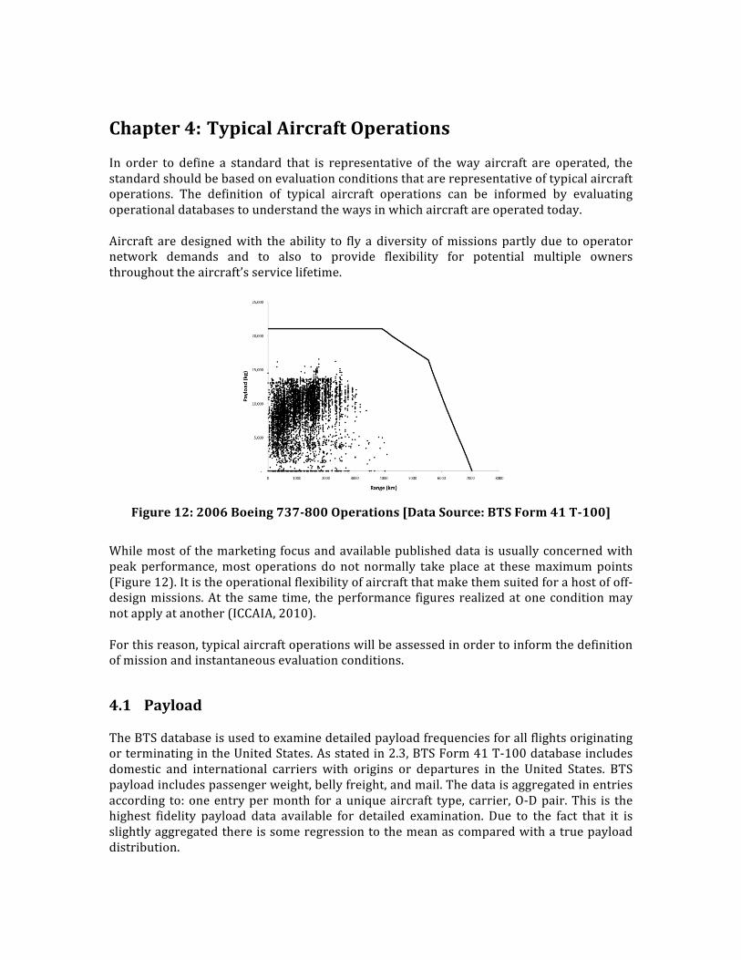
Chapter 4: Typical Aircraft Operations In order to define a standard that is representative of the way aircraft are operated, the standard should be based on evaluation conditions that are representative of typical aircraft operations. The definition of typical aircraft operations can be informed by evaluating operational databases to understand the ways in which aircraft are operated today. Aircraft are designed with the ability to fly a diversity of missions partly due to operator network demands and to also to provide flexibility for potential multiple owners throughout the aircraft’s service lifetime.
Figure 12: 2006 Boeing 737-800 Operations [Data Source: BTS Form 41 T-100]
While most of the marketing focus and available published data is usually concerned with peak performance, most operations do not normally take place at these maximum points (Figure 12). It is the operational flexibility of aircraft that make them suited for a host of off-‐design missions. At the same time, the performance figures realized at one condition may not apply at another (ICCAIA, 2010). For this reason, typical aircraft operations will be assessed in order to inform the definition of mission and instantaneous evaluation conditions.
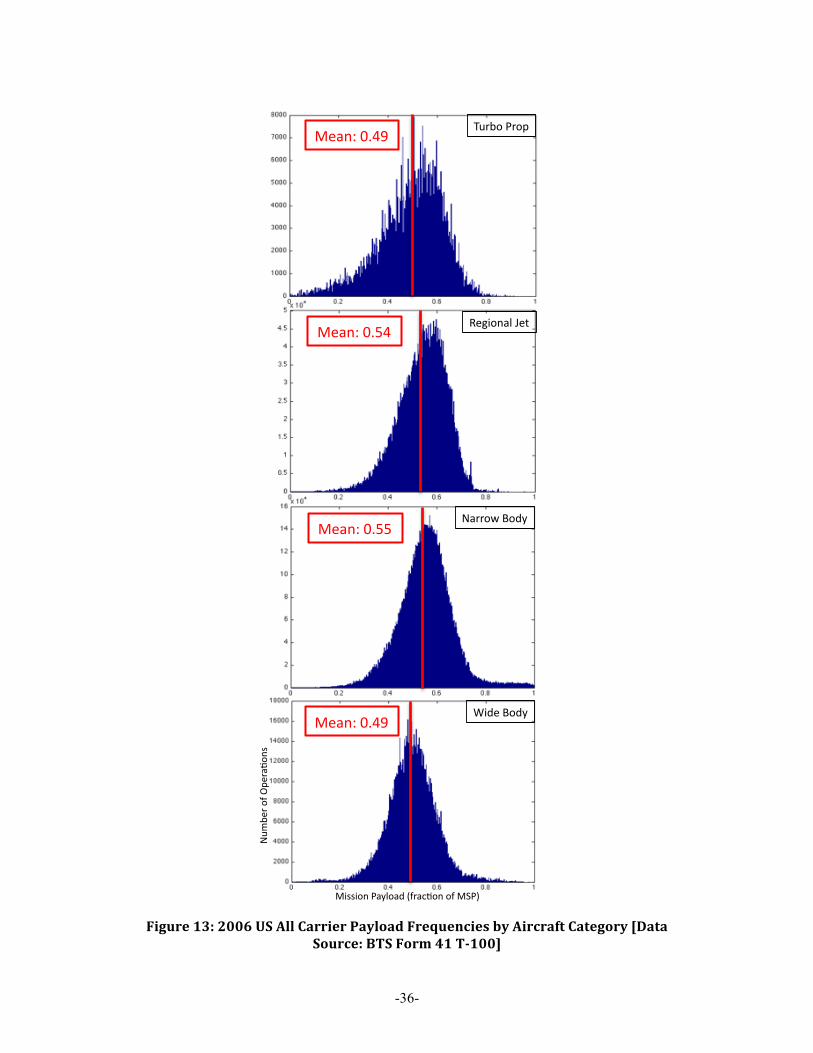
4.1 Payload The BTS database is used to examine detailed payload frequencies for all flights originating or terminating in the United States. As stated in 2.3, BTS Form 41 T-‐100 database includes domestic and international carriers with origins or departures in the United States. BTS payload includes passenger weight, belly freight, and mail. The data is aggregated in entries according to: one entry per month for a unique aircraft type, carrier, O-‐D pair. This is the highest fidelity payload data available for detailed examination. Due to the fact that it is slightly aggregated there is some regression to the mean as compared with a true payload distribution.
-36-
Figure 13: 2006 US All Carrier Payload Frequencies by Aircraft Category [Data
Source: BTS Form 41 T-100]
!"##"$%&'()*$(+&,-.(/0$%&$-&!1'2&
345
67.&$-&897
.(0$
%#&
:4.6$&'.$9&
;7<"$%(*&=7>&
3(..$?&@$+)&
A"+7&@$+)&!"#$%&'()*&
!"#$%&'(++&
!"#$%&'(+)&
!"#$%&'()*&

-37-
As seen in Figure 13, all payload frequencies are have a single mode, with an average frequency between 49% to 55% of MSP. The chart is ordered from top to bottom by (generally) shorter-‐range aircraft to longer-‐range aircraft.
4.2 Range The BTS database was used to assess range frequencies by aircraft type and category. An example range frequency is depicted in Figure 14 for a Boeing 737-‐800.
Figure 14: 2006 Boeing 737-800 Range Frequency [Data Source: BTS Form 41 T-100]
The Boeing 737-‐800 (with winglets) has an R1 range at 4,009km (Piano-‐X). As can be seen in Figure 14, approximately 97% of operations occur below R1 range. The distribution has a peak near 40% of R1 range. Absolute range frequency for the total fleet is shown in Figure 15.

-38-
Figure 15: 2006 Total Fleet US All Carrier Range Frequency [Data Source: BTS Form
41 T-100]
Most fleet missions occur below 5,000km mission range. This is due to the fact that all intra-‐US missions are less than this distance. Trans-‐Atlantic flights from the Northeastern United States to Western Europe are approximately 5,000km (BOS to LHR, 5,230km). The slight increase in frequency on missions of approximately 6,000km+ is due to trans-‐Atlantic flights from Southeastern and Mid/Mid-‐Western United States to Western Europe, all of US to Mid/Eastern Europe, and trans-‐Pacific flights. Range frequencies by aircraft category were computed and the results were aggregated into 500 bins based on fraction of R1 range for each aircraft type. The charts with relative distances (i.e. percent of R1) presented in this section include distances up to R1 range. On a fleet-‐wide basis, 1.7% of operations occur past R1 range (BTS, Piano-‐X).
Figure 16: 2006 Narrow Body Aircraft US All Carrier Range Frequency [Data Source:
BTS Form 41 T-100]
!"##"$%&'(%)*&+,-.&
/0-
1*2&$3&45*
2(6$
%#&
!"#$%
!"#$%&'()*&
-39-
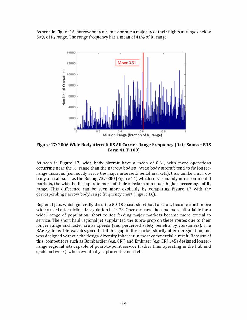
As seen in Figure 16, narrow body aircraft operate a majority of their flights at ranges below 50% of R1 range. The range frequency has a mean of 41% of R1 range.
Figure 17: 2006 Wide Body Aircraft US All Carrier Range Frequency [Data Source: BTS
Form 41 T-100]
As seen in Figure 17, wide body aircraft have a mean of 0.61, with more operations occurring near the R1 range than the narrow bodies. Wide body aircraft tend to fly longer-‐range missions (i.e. mostly serve the major intercontinental markets), thus unlike a narrow body aircraft such as the Boeing 737-‐800 (Figure 14) which serves mainly intra-‐continental markets, the wide bodies operate more of their missions at a much higher percentage of R1 range. This difference can be seen more explicitly by comparing Figure 17 with the corresponding narrow body range frequency chart (Figure 16). Regional jets, which generally describe 50-‐100 seat short-‐haul aircraft, became much more widely used after airline deregulation in 1978. Once air travel became more affordable for a wider range of population, short routes feeding major markets became more crucial to service. The short haul regional jet supplanted the tubro-‐prop on these routes due to their longer range and faster cruise speeds (and perceived safety benefits by consumers). The BAe Systems 146 was designed to fill this gap in the market shortly after deregulation, but was designed without the design diversity inherent in most commercial aircraft. Because of this, competitors such as Bombardier (e.g. CRJ) and Embraer (e.g. ERJ 145) designed longer-‐range regional jets capable of point-‐to-‐point service (rather than operating in the hub and spoke network), which eventually captured the market.
!"#$%&'()*&

-40-
Figure 18: April 2006 Regional Jet US All Carrier Range Frequency [Data Source: BTS
Form 41 T-100]
Due to these design considerations and the market that they serve, regional jets are operated with a mean frequency of 39% of R1 (Figure 18). Currently, amid competition from low cost carriers on midsize city pairs, regional jets are facing declining number of departures.
Figure 19: 2006 Turbo Prop US All Carrier Range Frequency [Data Source: BTS Form
41 T-100]
Turbo prop aircraft compete with regional jets by offering lower fuel consumption (but higher maintenance costs) and an ability to take off from shorter runways. However, the emergence of regional jets has pushed the turbo prop into very short-‐range markets, as exhibited by the mean range frequency at 30% of R1 range in Figure 19.
!"#$%&'()*&
!"#$%&'()'&
-41-
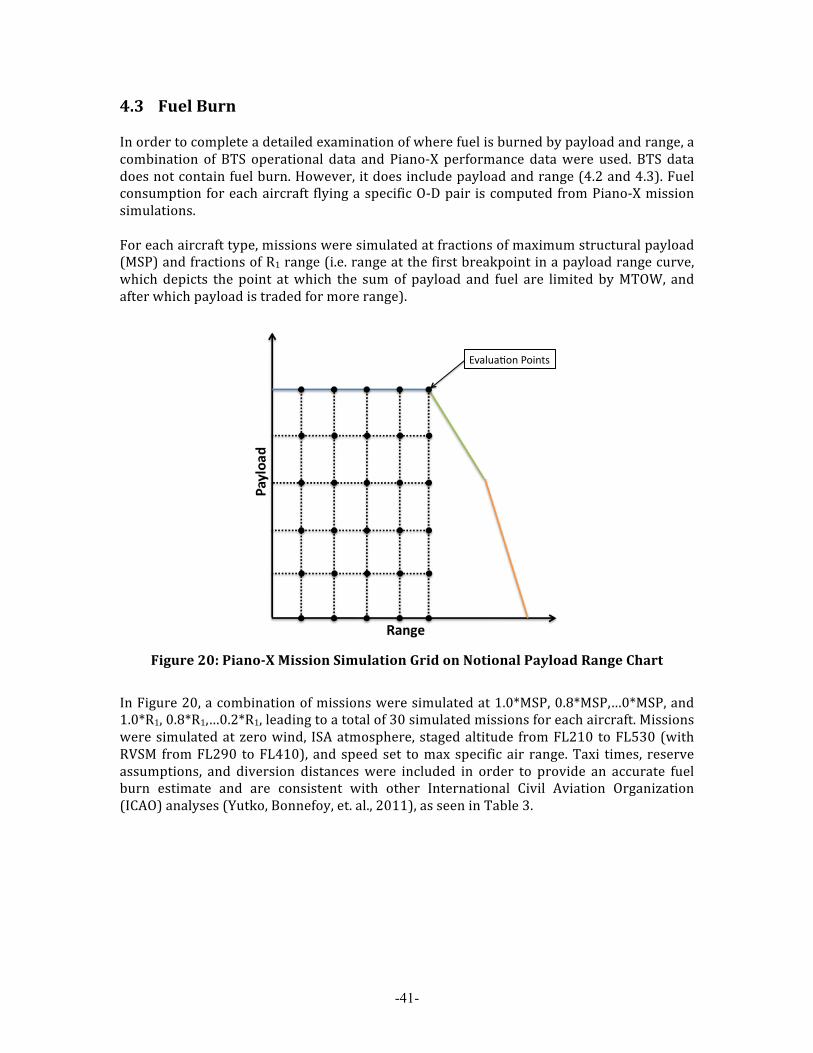
4.3 Fuel Burn In order to complete a detailed examination of where fuel is burned by payload and range, a combination of BTS operational data and Piano-‐X performance data were used. BTS data does not contain fuel burn. However, it does include payload and range (4.2 and 4.3). Fuel consumption for each aircraft flying a specific O-‐D pair is computed from Piano-‐X mission simulations. For each aircraft type, missions were simulated at fractions of maximum structural payload (MSP) and fractions of R1 range (i.e. range at the first breakpoint in a payload range curve, which depicts the point at which the sum of payload and fuel are limited by MTOW, and after which payload is traded for more range).
Figure 20: Piano-X Mission Simulation Grid on Notional Payload Range Chart
In Figure 20, a combination of missions were simulated at 1.0*MSP, 0.8*MSP,…0*MSP, and 1.0*R1, 0.8*R1,…0.2*R1, leading to a total of 30 simulated missions for each aircraft. Missions were simulated at zero wind, ISA atmosphere, staged altitude from FL210 to FL530 (with RVSM from FL290 to FL410), and speed set to max specific air range. Taxi times, reserve assumptions, and diversion distances were included in order to provide an accurate fuel burn estimate and are consistent with other International Civil Aviation Organization (ICAO) analyses (Yutko, Bonnefoy, et. al., 2011), as seen in Table 3.
!"#$%#&'()*'+(,-)
Table 3: Full Mission Piano-X Assumptions
Variable Assumption Atmosphere ISA
Taki-‐out/Takeoff/Approach/Taxi-‐in Piano-‐X Default7 Cruise Speed Schedule Maximum Range Cruise (MRC)
Cruise Altitude Schedule Staged Altitude from FL210 to FL530 (with RVSM from FL290 to FL410)
Contingency Fuel WB, NB (5%); Others (0%) Distance to Alternate WB, NB (370km); RJ and TP (185km); BJ (NBAA IFR:
370km for long-‐haul –185km for short-‐haul) Hold Time WB, NB, BJ (30min)
Given the grid of simulated fuel consumption by mission specification (payload and range), values of fuel burn for each aircraft type serving specific routes (range) at partial load factors (payload) were estimated using a bi-‐cubic interpolation algorithm (Figure 21).
Figure 21: Bi-Cubic Fuel Burn Interpolation
A heat map was used to visualize the fuel burn data computed by the bi-‐cubic interpolation algorithm. Each heat map is divided 100 times on each axis so that the map contains a 100x100 grid. Each grid is assigned a color that depicts the actual amount of total fuel consumed (kg) by aircraft that flew missions inside of that grid. Grids are either absolute (i.e. kg, km) or relative (%R1, %MSP). Due to the way in which fuel burn is computed, fuel burn data only includes mission up to R1 and MSP.
7 Piano-X default varies by aircraft type.
known fuel-burn:!performance data!
unknown fuel-burn: !actual operation point!

-43-
Figure 22: 2006 US All Carrier Fleet Wide Fuel Burn, Payload Frequency, and Range
Frequency [Data Source: BTS Form 41 T-100 and Piano-X]
As can be seen on Figure 22, most fleet fuel burn occurs near 10,000kg payload and 1,000km mission distance. The region of the fuel burn temperature map less than ~4,000 km indicates intra-‐US flights. The gap between ~4,000km and ~5,000km indicates the geographic difference between intra-‐US flights and intercontinental flights. As is evident by the frequency plots, there are significantly less international flights. However, these long-‐range flights burn a relatively high amount of fuel. The grids near 5,000km with 1.5e9kg of fuel burn have approximately 12 times less operations than an equivalent fuel burn grid on mission distances less than 5,000km.
!"#$%

-44-
Figure 23: Worldwide Fuel Burn, Payload, and Departures (Operations) by Aircraft
Type [Data Source: COD]
A majority of fleet-‐wide fuel burn, 54%, comes from narrow body aircraft8, while 38% comes from wide body aircraft. However, while wide bodies account for a smaller proportion of fuel burn, their fuel burn per flight is relatively very high as they are only 4% of departures (as opposed to 59% for narrow bodies).
Figure 24: 2006 US All Carrier Wide Body Fuel Burn, Payload Frequency, and Range
Frequency [Data Source: BTS Form 41 T-100 and Piano-X]
8 Here, narrow body is defined as SA and STA; Wide body is defined as LTA and LQ; see: 3.3 Aircraft Categories and Aircraft List
!"#
$!"#
%!"#
&!"#
'!"#
(!"#
)!"#
*!"#
+!"#
,!"#
$!!"#
-./0#1.23# 4560758# 9:/25;73<#
1=#
>=#
?4#
-#
@A#
@?B#
C?B#
CB#
!"#
$!"#
%!"#
&!"#
'!"#
(!"#
)!"#
*!"#
+!"#
,!"#
$!!"#
-./0#1.23# 4560758# 9:/25;73<#
1=#
>=#
?4#
-#
@A#
@?B#
C?B#
CB#
num
ber o
f ops!
Fuel Burn (kg)!
%R1!
%M
P!
Mean: 0.49 !
Mean: 0.61 !
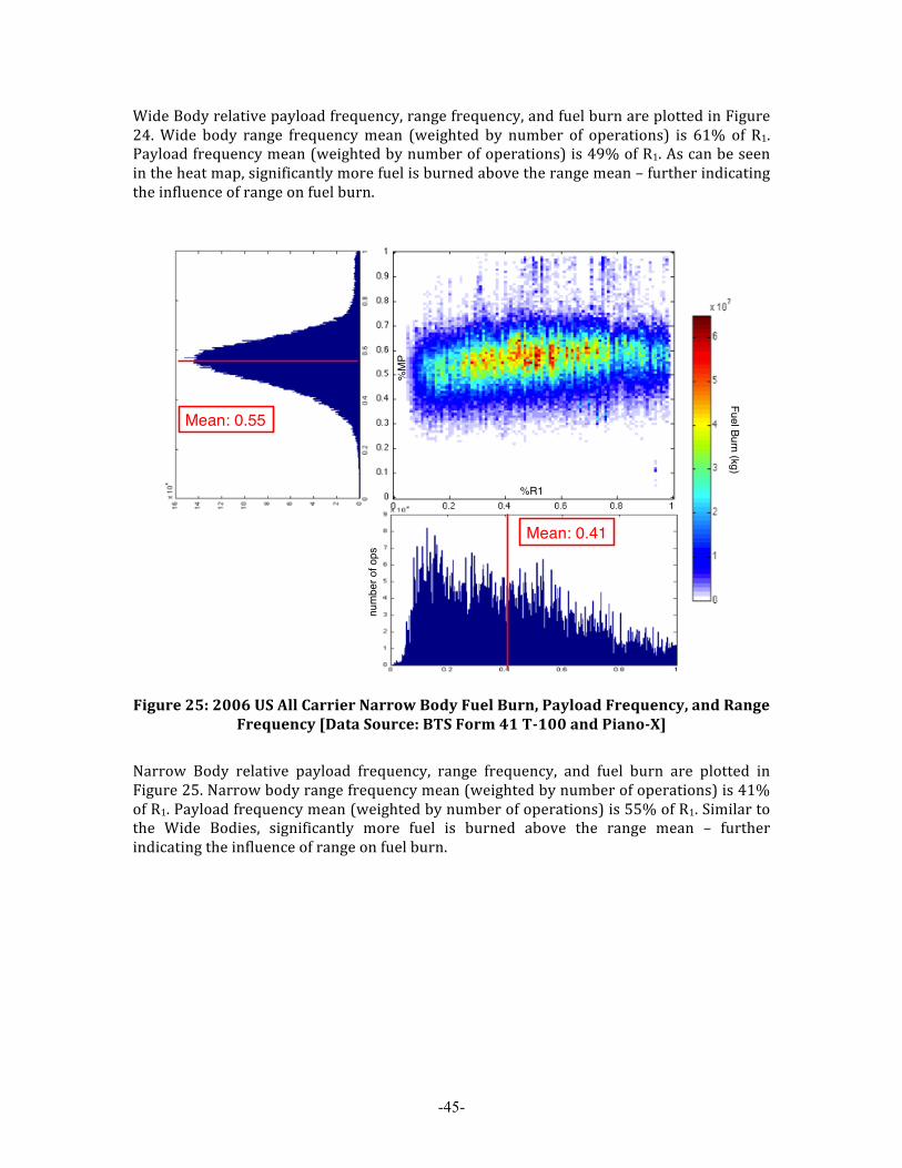
-45-
Wide Body relative payload frequency, range frequency, and fuel burn are plotted in Figure 24. Wide body range frequency mean (weighted by number of operations) is 61% of R1. Payload frequency mean (weighted by number of operations) is 49% of R1. As can be seen in the heat map, significantly more fuel is burned above the range mean – further indicating the influence of range on fuel burn.
Figure 25: 2006 US All Carrier Narrow Body Fuel Burn, Payload Frequency, and Range
Frequency [Data Source: BTS Form 41 T-100 and Piano-X]
Narrow Body relative payload frequency, range frequency, and fuel burn are plotted in Figure 25. Narrow body range frequency mean (weighted by number of operations) is 41% of R1. Payload frequency mean (weighted by number of operations) is 55% of R1. Similar to the Wide Bodies, significantly more fuel is burned above the range mean – further indicating the influence of range on fuel burn.
num
ber o
f ops!
Fuel Burn (kg)!
%R1!
%M
P!
Mean: 0.55 !
Mean: 0.41 !

-46-
Figure 26: 2006 US All Carrier Regional Jet Fuel Burn, Payload Frequency, and Range
Frequency [Data Source: BTS Form 41 T-100 and Piano-X]
Regional Jet relative payload frequency, range frequency, and fuel burn are plotted in Figure 26. Range frequency mean (weighted by number of operations) and payload frequency mean (weighted by number of operations) are very similar to Narrow Body aircraft (39% of R1 and 54% of MSP respectively), leading to a similar fuel burn profile.
!"#$%

-47-
Figure 27: 2006 US All Carrier Regional Jet Fuel Burn, Payload Frequency, and Range
Frequency [Data Source: BTS Form 41 T-100 and Piano-X]
Turbo Prop relative payload frequency, range frequency, and fuel burn are plotted in Figure 27. Turbo props are operated at a lower weighted average range (30% of R1) than other aircraft types but with a similar mean payload (49% of MSP). The fuel burn map less concentrated than other aircraft types. In Figure 22, most fleet wide range operations occur near 1,000km. This distance was used to examine fuel burn frequencies on missions longer and shorter by aircraft type.
Figure 28: April 2006 Global Operations Above and Below 1,000km by Percent
Departure (left) and Percent Fuel Burn (right) [Data Source: COD]
!"#$%
!"#
$!"#
%!"#
&!"#
'!"#
(!"#
)!"#
*!"#
+!"#
,!"#
$!!"#
-$!!!./#
01$!!!./#
!"#
$!"#
%!"#
&!"#
'!"#
(!"#
)!"#
*!"#
+!"#
,!"#
$!!"#
-$!!!./#
01$!!!./#
!"#$!"#%!"#&!"#'!"#(!"#)!"#*!"#+!"#,!"#$!!"#
-.# -/0# 1/0# 10# 23# /4# 53# /6789#!"#
$!"#%!"#&!"#'!"#(!"#)!"#*!"#+!"#,!"#
$!!"#
-.# -/0# 1/0# 10# 23# /4# 53# /6/0-#

-48-
Percentages of departures above and below 1,000km are depicted in the left side of Figure 28, while percentage of fuel burn for the same aircraft categories are shown on the right side. Percent fuel burn is less than percent departures on missions less than 1,000km for every aircraft category, indicating that missions over 1,000km are more fuel intensive. 82% of total fuel burn is from missions over 1,000km, which only comprise 42% of departures.
Figure 29: April 2006 World Wide Operations: % of Total Fuel Burned on Missions
+/- 1,000km by Aircraft Type [Data Source: COD]
Figure 29 shows percentage of total fuel burn on missions above and below 1,000km by aircraft type. Wide bodies and turbo props exhibit a small distribution of fuel burn across aircraft types, illustrating that, on a fuel burn basis, wide bodies and turboprops are less operationally diverse. The opposite is true for narrow bodies and regional jets, which exhibit a large difference amongst each aircraft category. A detailed list April 2006 global fuel burn above and below 1,000km by aircraft type is included in Figure 30.
!"#
$!"#
%!"#
&!"#
'!"#
(!"#
)!"#
*!"#
+!"#
,!"#
$!!"#
(SA)!
% o
f Tot
al F
uel B
urn!
!"#
$!"#
%!"#
&!"#
'!"#
(!"#
)!"#
*!"#
+!"#
,!"#
$!!"#
-$!!!./#
01$!!!./#
(LQ)!(LTA)! (STA)! (RJ)! (TP)! (BJ)!
Large Quad !(LQ)!Large Twin Aisle !(LTA)!Small Twin Aisle !(STA)!Single Aisle !(SA)!Regional Jet !(RJ)!Turbo Prop !(TP)!Business Jet !(BJ)!
(Each Bar Represents a Single
Aircraft Type)!

-49-
!"# $!"# %!"# &!"# '!"# (!"# )!"# *!"# +!"# ,!"# $!!"#
-*'*./0#
-*'*.'12#
-*'*.%#
-*'*.'#
-*'*.&#
-*'*.$#
-*'*./2#
3&'!.%#
3&'!.)#
3&'!.&#
45$$#
-***.%12#
45$$.12#
3&&!.%#
3&'!.(#
-***.&12#
3&&!.&#
-***.%#
45$!.&#
-***.&#
!"#
$!"#
%!"#
&!"#
'!"#
(!"#
)!"#
*!"#
+!"#
,!"#
$!!"#
-$!!!./#
01$!!!./#
!"#
$!"#
%!"#
&!"#
'!"#
(!"#
)!"#
*!"#
+!"#
,!"#
$!!"#
-$!!!./#
01$!!!./#
!"# $!"# %!"# &!"# '!"# (!"# )!"# *!"# +!"# ,!"# $!!"#
-*'*./0#
-*'*.'12#
-*'*.%#
-*'*.'#
-*'*.&#
-*'*.$#
-*'*./2#
3&'!.%#
3&'!.)#
3&'!.&#
45$$#
-***.%12#
45$$.12#
3&&!.%#
3&'!.(#
-***.&12#
3&&!.&#
-***.%#
45$!.&#
-***.&#
!"#
!$%#
!"# $!"# %!"# &!"# '!"# (!"# )!"# *!"# +!"# ,!"# $!!"#
-*)*.'/0#
12$!.'#
3$!$$.&#
12$!.&/0#
-*)*.'#
12$!.&#
-*(*.&#
-*)*.%/0#
-*)*.&/0#
4&$!.&#
-*(*.%#
12$!.$#
-*)*.%#
4&!!2'.)#
-*%*.%0/.567/0%*#
4&$!.%#
-*)*.&#
4&!!-'.)#
4&!!-'.%#
4&!!-'.$#
-*%*.%#
-*%*.$#
4&!!-%.%#
4&!!-%8.&#
&$%#
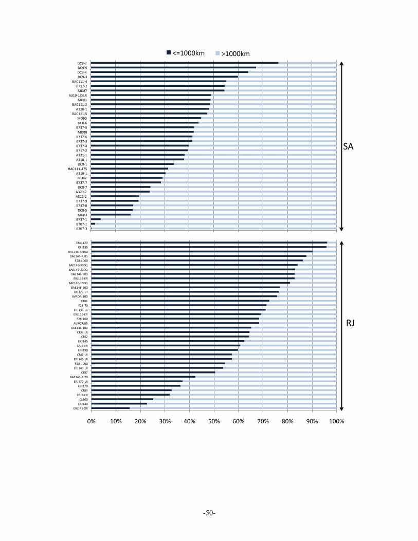
-50-
!"# $!"# %!"# &!"# '!"# (!"# )!"# *!"# +!"# ,!"# $!!"#
-./$'(01.#-./$'!#23)!!#
2./*0-.#2./,#
-./$*!#-./$*!03.#
45-$')0./*!#2./*#
-./$'!03.#6%+0$!!!#-./$'(03.#2./$03.#-./$,!#2./%0-.#-./$'(#2./%#
2./%03.#45-$')0$!!#57.8./+(#6%+0$!!#
-./$&(0-.#-./$&(03.#
6%+0*!#2./$#
57.8./$!!#98&%+/-:#
45-$')0%!!#45-$')0$!!;#
-./$'(0-.#45-$')0&!!#
45-$')0%!!;#45-$')0&!!;#
6%+0'!!!#45-$')0./+(#
45-$')0./$!!#-./$&(#
-<4$%!#!"# $!"# %!"# &!"# '!"# (!"# )!"# *!"# +!"# ,!"# $!!"#
-*!*.&#-*!*.$#-*&*.$#/0++.(#-*&*.+#-*&*.,#2&%$.%#2&%!.%#01+.*#-*&*.*#/0+%#2&$,.$#
-21$$$.'*(#01,.$#2&$+.$#2&%$.$#-*$*.%#-*&*.'#-*&*.&#-*&*.)#/0++#-*&*.(#01+.)#/0,!#
-21$$$.(#2&%!.$#
-21$$$.%#/0+$#
2&$,.$3456#/0+*#-*&*.%#
-21$$$.'#01,.,.'#01,.(#01,.%#
!"#
$!"#
%!"#
&!"#
'!"#
(!"#
)!"#
*!"#
+!"#
,!"#
$!!"#
-$!!!./#
01$!!!./#
!"#
$!"#
%!"#
&!"#
'!"#
(!"#
)!"#
*!"#
+!"#
,!"#
$!!"#
-$!!!./#
01$!!!./#
!"#
$%#

-51-
Figure 30: April 2006 Percentage of Fuel Burn +/- 1,000km by Aircraft Type [Data
Source: COD]
!"# $!"# %!"# &!"# '!"# (!"# )!"# *!"# +!"# ,!"# $!!"#
-./01.2345266#
-7.8(#
-7.8%#
-7.8'964#
-7.8%90#
-7.8'#
-7.8%964#
-7.8&#
81.,!!0#
81.,!!:#
-7.8%!!#
81.(!923#
81.,!!#
0*&*9*900;#
<6$%(9*#
<6$%(9+#
81.(!#
81.%!92#
81.%!98#
81.%!9=#
81.%!!#
81.%!9:#
81.%!9-#
:>1((!#
:>1((!96#!"# $!"# %!"# &!"# '!"# (!"# )!"# *!"# +!"# ,!"# $!!"#
-./'%0&#
12234%!!#
-./'%0&%!#
5--1%!!!#
6%*0$#
5-%%*#
5-%%)#
743+80'#
-./'%0%#
5--1&'!01#
5--1&'!019#
7:&%+0$#
5--1&'!0-#
-./'%0'#
-./'%0(#
-./*%0%#
12234$,!!07#
12234$,!!03#
743+80$#
743+0$#
743+0&#
743+80&#
6%*0(!#
743+0%#
743+80%#
!"#
$!"#
%!"#
&!"#
'!"#
(!"#
)!"#
*!"#
+!"#
,!"#
$!!"#
-$!!!./#
01$!!!./#
!"#
$!"#
%!"#
&!"#
'!"#
(!"#
)!"#
*!"#
+!"#
,!"#
$!!"#
-$!!!./#
01$!!!./#
!"#
$%#

Figure 31 further illustrates that a significant portion of fleet-‐wide fuel burn is due to long-‐range missions.
Figure 31: April 2006 Cumulative Distribution of Fuel Burn, Payload, and Departures
[Data Source: COD]
For example, 86% of fleet-‐wide departures happen at or below 2,000km mission distance while only consuming 40% of fleet-‐wide fuel burn. 60% of fleet fuel burn comes from missions over 2,000km, while only consisting of 14% of fleet-‐wide departures.
Figure 32: Fuel Burn by Phase of Flight for Each Aircraft Category [Data source: COD]
!"#
$!"#
%!"#
&!"#
'!"#
(!"#
)!"#
*!"#
+!"#
,!"#
$!!"##-####
#$.!!!
##
#%.!!!
##
#&.!!!
##
#'.!!!
##
#(.!!!
##
#).!!!
##
#*.!!!
##
#+.!!!
##
#,.!!!
##
#$!.!!
!##
#$$.!!
!##
#$%.!!
!##
#$&.!!
!##
#$'.!!
!##
#$(.!!
!##
#$).!!
!##
/012#3045# 678297:# ;1<74=041>#
!"#
$!"#
%!"#
&!"#
'!"#
(!"#
)!"#
*!"#
+!"#
,!"#
$!!"#
#-####
#$.!!!
##
#%.!!!
##
#&.!!!
##
#'.!!!
##
#(.!!!
##
#).!!!
##
#*.!!!
##
#+.!!!
##
#,.!!!
##
#$!.!!
!##
#$$.!!
!##
#$%.!!
!##
#$&.!!
!##
#$'.!!
!##
#$(.!!
!##
#$).!!
!##
/012#3045# 678297:# ;1<74=041>#
Mission Distance (km)!
Cum
ulat
ive
Dis
trib
utio
n:!
% o
f Tot
al (a
ttrib
ute)
on
Mis
sion
s at
or B
elow
Dis
tanc
e!(e
.g. 5
0% o
f tot
al fl
eet f
uel b
urn
is c
onsu
med
on
mis
sion
s <
2,90
0km
)!
!"#
$!"#
%!"#
&!"#
'!"#
(!"#
)!"#
*!"#
+!"#
,!"#
$!!"#
-.# -/.# 0/.# 01# 2# /3# 45# 65#
.7789:;#2<=;#6<7>#?@20$!!A#
2<=;#6<7>#?B20$!!A#
C=D:7E<7=#2<=;#6<7>#?@20$!!A#
!"#
$!"#
%!"#
&!"#
'!"#
(!"#
)!"#
*!"#
+!"#
,!"#
$!!"#
-.# -/0# 1/0# 10# 23# /4# 53#

-53-
Climb is an inherently less ‘efficient’ phase than cruise because the aircraft is expending energy to increase its potential energy (altitude). As is expected, short-‐range aircraft tend to burn relatively more fuel during climb than long-‐range aircraft (Figure 32).
4.4 Takeoff Weights In order to inform the definition of a SAR evaluation weight, it is useful to understand the frequency takeoff weights. Takeoff weight (see: Figure 10) was computed by adding the aircraft OEW to the payload and fuel burn for the mission, as calculated by the bi-‐cubic interpolation.
Figure 33: Histogram of Useful Load at Takeoff by Aircraft Category [Data Source: BTS
Form 41 T-100 and Piano-X]
Average useful load at takeoff (weighted average by number of departures) is approximately similar across all aircraft categories. A few business jets (Citation III) flew very low payload load factors in 2006 (~10% MSP) which skewed the business jet useful load average to the left.
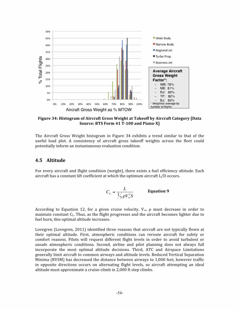
-54-
Figure 34: Histogram of Aircraft Gross Weight at Takeoff by Aircraft Category [Data
Source: BTS Form 41 T-100 and Piano-X]
The Aircraft Gross Weight histogram in Figure 34 exhibits a trend similar to that of the useful load plot. A consistency of aircraft gross takeoff weights across the fleet could potentially inform an instantaneous evaluation condition.
4.5 Altitude For every aircraft and flight condition (weight), there exists a fuel efficiency altitude. Each aircraft has a constant lift coefficient at which the optimum aircraft L/D occurs.
€
CL =L
12 ρV∞
2S Equation 9
According to Equation 12, for a given cruise velocity, V∞, ρ must decrease in order to maintain constant CL. Thus, as the flight progresses and the aircraft becomes lighter due to fuel burn, this optimal altitude increases. Lovegren (Lovegren, 2011) identified three reasons that aircraft are not typically flown at their optimal altitude. First, atmospheric conditions can reroute aircraft for safety or comfort reasons. Pilots will request different flight levels in order to avoid turbulent or unsafe atmospheric conditions. Second, airline and pilot planning does not always full incorporate the most optimal altitude decisions. Third, ATC and Airspace Limitations generally limit aircraft to common airways and altitude levels. Reduced Vertical Separation Minima (RVSM) has decreased the distance between airways to 1,000 feet, however traffic in opposite directions occurs on alternating flight levels, so aircraft attempting an ideal altitude must approximate a cruise-‐climb in 2,000 ft step climbs.
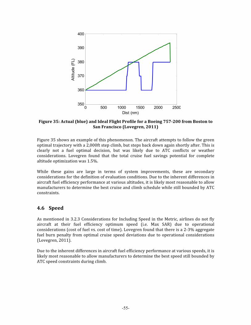
-55-
Figure 35: Actual (blue) and Ideal Flight Profile for a Boeing 757-200 from Boston to
San Francisco (Lovegren, 2011)
Figure 35 shows an example of this phenomenon. The aircraft attempts to follow the green optimal trajectory with a 2,000ft step climb, but steps back down again shortly after. This is clearly not a fuel optimal decision, but was likely due to ATC conflicts or weather considerations. Lovegren found that the total cruise fuel savings potential for complete altitude optimization was 1.5%. While these gains are large in terms of system improvements, these are secondary considerations for the definition of evaluation conditions. Due to the inherent differences in aircraft fuel efficiency performance at various altitudes, it is likely most reasonable to allow manufacturers to determine the best cruise and climb schedule while still bounded by ATC constraints.
4.6 Speed As mentioned in 3.2.3 Considerations for Including Speed in the Metric, airlines do not fly aircraft at their fuel efficiency optimum speed (i.e. Max SAR) due to operational considerations (cost of fuel vs. cost of time). Lovegren found that there is a 2-‐3% aggregate fuel burn penalty from optimal cruise speed deviations due to operational considerations (Lovegren, 2011). Due to the inherent differences in aircraft fuel efficiency performance at various speeds, it is likely most reasonable to allow manufacturers to determine the best speed still bounded by ATC speed constraints during climb.
16
right, the calculated airspeed in Mach. The blue lines represent the actual path flown, while the
green represents the optimal path. This flight representsof the forces at play. In due diligence,
the pilot makes a 2,000 step up at about 1,200 nm into the flight, the smallest increment
possible under RVSM. This step is in line with staying as close to optimal as is possible.
Unfortunately, at approximately 1,500 nm, the pilot steps down again. Clearly this was not a
performance enhancing choice—most likely this diversion was caused by ATC due to a traffic
conflict, or by turbulence at the higher flight level that the pilot hoped to escape by returning to
the last known smooth flight level. The speed profile illustrates a trend all too common in
today’s cruise operations: flying fast. Despite some noise in the data, it is clear the aircraft was
traveling at approximately Mach 0.80 when the best economy speed for the 757 is
approximately Mach 0.76.
Figure 1. Actual and ideal flight profiles for a Boeing 757-200 from Boston to San Francisco.
Another sample cruise flight profile is shown in Figure 2. This flight represents a shorter
trip of a Boeing 737-700 from Los Angeles to Chicago. In this altitude profile, the aircraft
remained at FL390 for the entirety of the flight. As fuel was burned, however, the ideal altitude
rose to over FL400. Whether or not the pilot intended to seek the optimal altitude condition is
not known, because step climbs of 1,000 ft are not normally given under current RVSM
0 500 1000 1500 2000 2500350
360
370
380
390
400
Dist (nm)
Alti
tude
(FL)
0 500 1000 1500 2000 25000.55
0.6
0.65
0.7
0.75
0.8
0.85
0.9
0.95
Dist (nm)
Mac
h
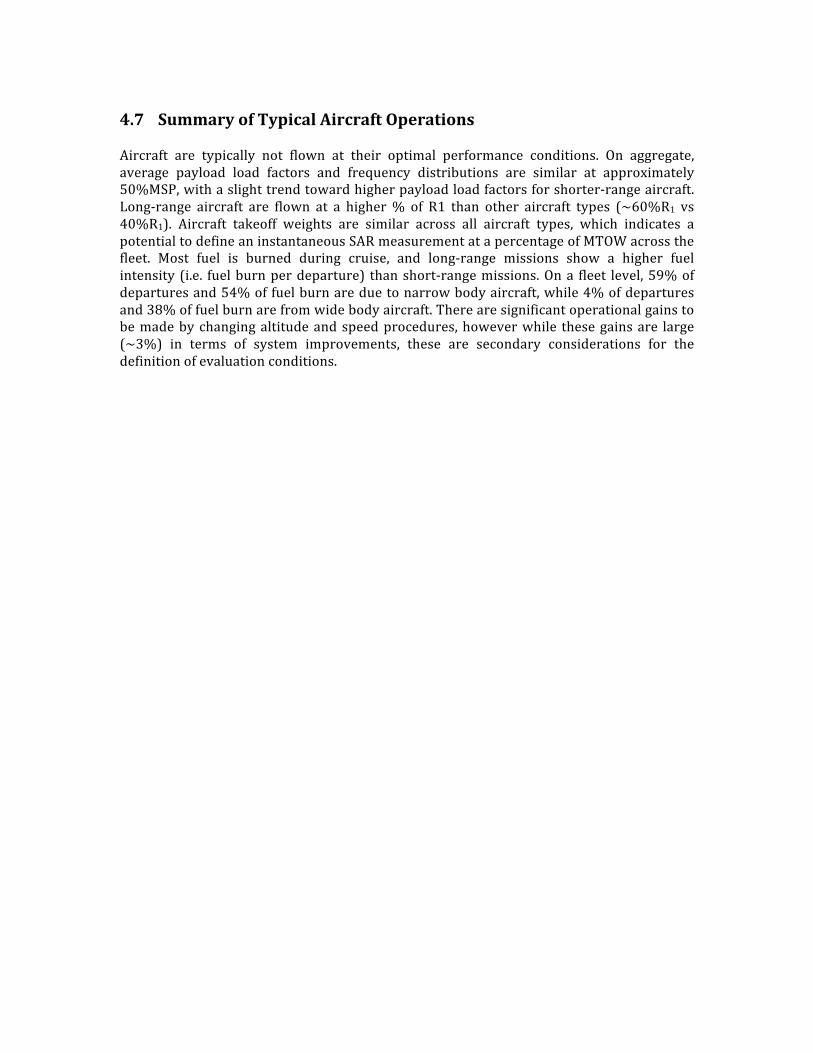
4.7 Summary of Typical Aircraft Operations Aircraft are typically not flown at their optimal performance conditions. On aggregate, average payload load factors and frequency distributions are similar at approximately 50%MSP, with a slight trend toward higher payload load factors for shorter-‐range aircraft. Long-‐range aircraft are flown at a higher % of R1 than other aircraft types (~60%R1 vs 40%R1). Aircraft takeoff weights are similar across all aircraft types, which indicates a potential to define an instantaneous SAR measurement at a percentage of MTOW across the fleet. Most fuel is burned during cruise, and long-‐range missions show a higher fuel intensity (i.e. fuel burn per departure) than short-‐range missions. On a fleet level, 59% of departures and 54% of fuel burn are due to narrow body aircraft, while 4% of departures and 38% of fuel burn are from wide body aircraft. There are significant operational gains to be made by changing altitude and speed procedures, however while these gains are large (~3%) in terms of system improvements, these are secondary considerations for the definition of evaluation conditions.

Chapter 5: Evaluation Conditions for a Full Mission Metric Definition of a full mission metric requires assumptions with regard to many parameters. However, while attributes such as speed and altitude (and to a lesser extent: taxi time, operational equipment, etc) do have an effect on day-‐to-‐day fuel burn (see: 4.5 and 4.6), the main driver for fuel burn is range (Figure 31). In this chapter, potential evaluation conditions with regard to range are identified based on their ability to represent typical aircraft operations while reducing the manufacturer burden of certification.
5.1 Fuel Efficiency Performance Sensitivity to Evaluation Conditions Measured fuel efficiency performance changes based on the evaluation condition at which the performance is measured. As an example, BF/R is evaluated at two different range conditions as shown in Figure 36.
Figure 36: BF/R vs MTOW Evaluated at Two Different Range Conditions [Data Source:
Piano-X]
In Figure 36, the same metric, CP, and payload (BF/R vs MTOW at MSP) is evaluated for the full Piano-‐X aircraft fleet using two different range assumptions. R1 is used as a proxy for design range, and 40% of R1 is used to approximate the range frequency most commonly found in typical operations (Figure 17-‐Figure 19). A single power law regression is used as a notional stringency or regulatory limit. The single regression is based on fleet-‐wide data rather than multiple regressions for each aircraft category. This is for simplification of the illustrative example and also to avoid the unintended consequences identified through literature review of the CAFE standard (10.1.2 Corporate Average Fuel Economy (CAFE)) (i.e. emergence of SUV’s). In a practical sense, the “regulatory incentive” from the standard comes from an aircraft’s margin to the regulatory limit.
!"#"$%$&'()$%(*+&",-"#"$%*./+0"
!"!!!!
!#$%%!!
!&$%%!!
!'$%%!!
!($%%!!
!)%$%%!!
!)#$%%!!
!)&$%%!!
!)'$%%!!
!"!!!! !)%*%%%!! !#%*%%%!! !+%*%%%!! !&%*%%%!! !,%*%%%!! !'%*%%%!! !-%*%%%!! !(%*%%%!!
123,"4567897:;<
"7:",
/"7=
<">?@A"
>BCD"
!"#"$%$&'()$%(*$*"+,"#"$%-.-&/"
!"!!#
$"!!#
%"!!#
&"!!#
'"!!#
(!"!!#
($"!!#
(%"!!#
(&"!!#
#)#### #(!*!!!## #$!*!!!## #+!*!!!## #%!*!!!## #,!*!!!## #&!*!!!## #-!*!!!## #'!*!!!##
012+"34567869:;
"69"$
%&+*
"6<;
"=>?@"
=ABC"

-58-
Figure 37: Margin to Regression Line [Data Source: Piano-X]
An aircraft with a large positive margin (Figure 37) is in less danger of failing the certification standard for future variants or for new aircraft derivatives, thus the manufacturer has less regulatory incentive to improve their aircraft. Margin is expressed as a residual from the regression line,
Equation 10
where R is the value of the regression line and M is the value of the metric at that point (Equation 10). Aircraft were ranked from worst (#1) to best (#214) by margin to the regression line for each evaluation condition. In Figure 38, the ranking for evaluation at R1 is plotted against the ranking for evaluation at 40% of R1. Aircraft on the line of equivalent ranking had the same ranking on both evaluation conditions. The amount of deviation from this line indicates that the two evaluation conditions rank the aircraft very differently. This implies that the certified performance changes based on the definition of the mission evaluation condition. Thus, the evaluation condition must be defined using defendable rationale.
!"!!!!
!#$%%!!
!&$%%!!
!'$%%!!
!($%%!!
!)%$%%!!
!)#$%%!!
!)&$%%!!
!)'$%%!!
!"!!!! !)%*%%%!! !#%*%%%!! !+%*%%%!! !&%*%%%!! !,%*%%%!! !'%*%%%!! !-%*%%%!! !(%*%%%!!
!"#$%&'()*+),-.
%),%$
/%)0
.%1234%
1567%
!"#$%&'()*+,$-(."(/',+'##$"-(0$-'(
1',*%&'()*+,$-(."(/',+'##$"-(0$-'(
!
margin =R "MR
!!"#$%&'

-59-
Figure 38: Aircraft Ranked by Residual for Two Different Evaluation Conditions [Data
Source: Piano-X]
One method for developing defendable rationale and assumptions is to ensure the evaluation condition represents typical aircraft operations.
5.2 Principle for Constructing Weighted Metric In order to more closely represent typical aircraft operations, a fuel efficiency metric can be weighted by operational frequencies (e.g. range) or impact (e.g. fuel burn). By doing this, the metric can more closely represent typical day-‐to-‐day operations. The weighted metric can also be compared to a non-‐weighted metric to understand if the single point (non-‐operations based metric) would have sufficiently measured performance, ex post facto. A “weighted metric” is a metric that is evaluated at multiple points and weighted at those points by operational frequency or impact.
Figure 39: Principle for Constructing Weighted Metric
!"#$%&'("
&)%&$'*+#',-"./"0+
&'"1'(
2'
!"#$%&'("&)%&$'*+#',-"./"0+&'"1'345'+*'(2'
=!M 2006 ops, B737-800 != 0.0073 !
COD!!"#$%&
'& ()*+,-.*/&
(*.0+1&
20*3
4*5
16&

-60-
Figure 39 shows a notional example of weighting a metric based on an operational frequency. On the left, a metric is evaluated at fractions of R1 range using Piano. On the right, operational frequencies are binned with centers on the locations of the piano evaluation points. The weighted metric is computed by performing a sum product of these two quantities (Equation 14).
€
MW = f0.2*R1 *M0.2*R1( ) + f0.4*R1 *M0.4*R1( ) + ...+ fR1 *MR1( ) Equation 11
5.3 Full Mission Metric Weighted by Range Frequency Range has the largest effect on aircraft fuel burn. J.E. Green found that “Payload Fuel Efficiency” (defined as payload*range/fuel_burn) declines significantly after 4,000km due to the need to carry extra fuel simply to carry the fuel for a long-‐range mission (Green, August 2006).
Figure 40: Fuel Efficiency Performance for Aircraft Types as a Function of R1 Range
[Data Source: PIANO-X] (Bonnefoy Y. M., 2011)
As demonstrated in Figure 40, the cutoff between aircraft with best BF/P*R fuel efficiency performance at R1 versus aircraft with best fuel efficiency performance at a range less than R1 is approximately 4,000km. Thus, aircraft with an R1 range less than 4,000km will have best fuel efficiency performance at R1, while aircraft with longer R1 ranges will have a best fuel efficiency performance point at some distance less than R1. Also, Figure 31 clearly demonstrates the impact of long-‐range missions on total fleet fuel burn. For these reasons, the range evaluation condition should exhibit an ability to reflect typical operations.
!"#$#%&'()*+,'-"./'0+,.'12+3'45$"+6$)'7+#89#:%6$+'

-61-
Range frequencies from Chapter 4:Typical Aircraft Operations and Piano performance data were used to compute the weighted metric in Equation 14. Figure 41 attempts to capture the differences between the weighted metric and a single-‐condition non-‐weighted metric (e.g. BF/R evaluated at R1) by dividing the two. The single evaluation condition metric “over states” the performance of aircraft above 1, while it “under states” the performance of the aircraft below 1. The standard is not meant to be predictive of operational performance, however, if different classes of aircraft are under and overstated differently based on the evaluation condition, then the evaluation condition fails to be equitable across stakeholders and represent typical operations.
Figure 41: Weighted Metric Normalized by Single Evaluation Condition Metric (R1) by
Aircraft Type
It is clear that the single evaluation condition at R1 overstates the performance of short-‐range aircraft. This is due to the fact that short-‐range aircraft have a fuel efficiency optimal point at R1, while their operations at ranges significantly less than R1 (Figure 16-‐Figure 19). Likewise, long range aircraft, which have an optimal performance point somewhere less than R1, are understated by a single point evaluation at R1. Sensitivity to evaluation condition is shown by comparing the weighted metric to metrics computed at 20% steps of R1 range. In Figure 42, the results are shown with a best-‐fit log trend line. Each log trend line is the weighted metric divided by a single-‐condition non-‐weighted metric.
!"#$
!"%$
!"&$
'$
'"'$
'"($
'")$
'"*$
!$ (!!!$ *!!!$ +!!!$ %!!!$ '!!!!$ '(!!!$ '*!!!$
!"#!
$%&'(
%&(%)*+,($-!'(
,-."/0120/!"(3'44$
,-."/0120/!"*3'44$
,-."/0120/!"+3'44$
,-."/0120/!"%3'44$
,-."/0120/3'44$!"#$
!"%$
!"&$
'$
'"'$
'"($
'")$
'"*$
!$ (!!!$ *!!!$ +!!!$ %!!!$ '!!!!$ '(!!!$ '*!!!$
!"#!
$%&'()*+,-
&'./+
01+02'(*+$3!/+
,-."/0120/!"(3'44$
,-."/0120/!"*3'44$
,-."/0120/!"+3'44$
,-."/0120/!"%3'44$
,-."/0120/3'44$
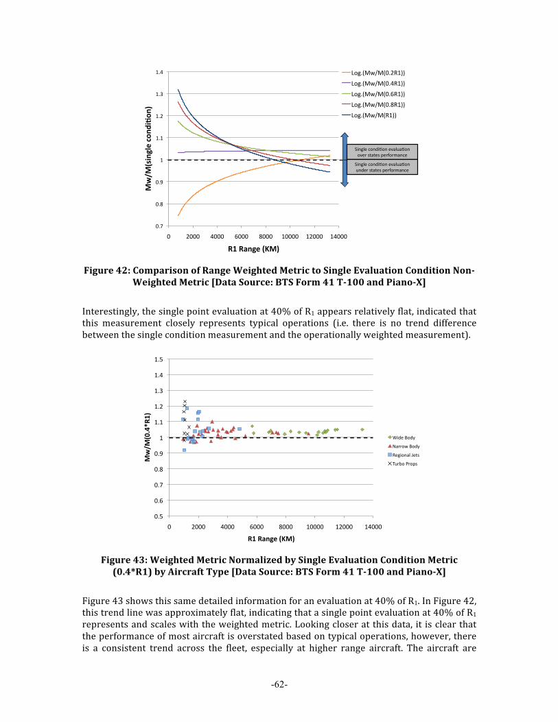
-62-
Figure 42: Comparison of Range Weighted Metric to Single Evaluation Condition Non-
Weighted Metric [Data Source: BTS Form 41 T-100 and Piano-X]
Interestingly, the single point evaluation at 40% of R1 appears relatively flat, indicated that this measurement closely represents typical operations (i.e. there is no trend difference between the single condition measurement and the operationally weighted measurement).
Figure 43: Weighted Metric Normalized by Single Evaluation Condition Metric (0.4*R1) by Aircraft Type [Data Source: BTS Form 41 T-100 and Piano-X]
Figure 43 shows this same detailed information for an evaluation at 40% of R1. In Figure 42, this trend line was approximately flat, indicating that a single point evaluation at 40% of R1 represents and scales with the weighted metric. Looking closer at this data, it is clear that the performance of most aircraft is overstated based on typical operations, however, there is a consistent trend across the fleet, especially at higher range aircraft. The aircraft are
!"#$
!"%$
!"&$
'$
'"'$
'"($
'")$
'"*$
!$ (!!!$ *!!!$ +!!!$ %!!!$ '!!!!$ '(!!!$ '*!!!$
!"#!
$%&'()*+,-
&'./+
01+02'(*+$3!/+
,-."/0120/!"(3'44$
,-."/0120/!"*3'44$
,-."/0120/!"+3'44$
,-."/0120/!"%3'44$
,-."/0120/3'44$
!"#$
!"%$
!"&$
'$
'"'$
'"($
'")$
'"*$
!$ (!!!$ *!!!$ +!!!$ %!!!$ '!!!!$ '(!!!$ '*!!!$
!"#!
$%&'()*+,-
&'./+
01+02'(*+$3!/+
,-."/0120/!"(3'44$
,-."/0120/!"*3'44$
,-."/0120/!"+3'44$
,-."/0120/!"%3'44$
,-."/0120/3'44$
!"#$
!"%$
!"&$
'$
'"'$
'"($
'")$
'"*$
!$ (!!!$ *!!!$ +!!!$ %!!!$ '!!!!$ '(!!!$ '*!!!$
!"#!
$%&'()*+,-'.
&/-'
0+
12+13'(*+$4!0+
,-."/0120/!"(3'44$
,-."/0120/!"*3'44$
,-."/0120/!"+3'44$
,-."/0120/!"%3'44$
,-."/0120/3'44$
!"#$%&'()#*"+)#'&,-%.-+)#''),&/'01-1&0'2&/3)/4-#(&'
!"#$%&'()#*"+)#'&,-%.-+)#''.#*&/'01-1&0'2&/3)/4-#(&'
!"#$
!"%$
!"&$
!"'$
!"($
)$
)")$
)"*$
)"+$
)",$
)"#$
!$ *!!!$ ,!!!$ %!!!$ '!!!$ )!!!!$ )*!!!$ ),!!!$
!"#!
$%&'()
*+,
)*,)-./0,$1!+,
-./0$12/3$
456627$12/3$
809.2:5;$<0=>$
?@6A2$B62C>$
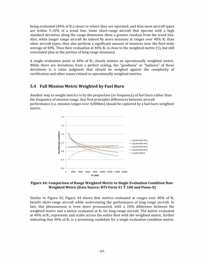
-63-
being evaluated (40% of R1) closer to where they are operated, and thus most aircraft types are within 5-‐10% of a trend line. Some short-‐range aircraft that operate with a high standard deviation along the range dimension show a greater residual from the trend line. Also, while longer range aircraft do indeed fly more missions at ranges over 40% R1 than other aircraft types, they also perform a significant amount of missions near the fleet-‐wide average of 40%. Thus their evaluation at 40% R1 is close to the weighted metric (1), but still overstated (due to the portion of long range missions). A single evaluation point at 40% of R1 closely mimics an operationally weighted metric. While there are deviations from a perfect scaling, the “goodness” or “badness” of these deviations is a value judgment that should be weighed against the complexity of certification and other issues related to operationally weighted metrics.
5.4 Full Mission Metric Weighted by Fuel Burn Another way to weight metrics is by the proportion (or frequency) of fuel burn rather than the frequency of mission range. Any first principles differences between aircraft performance (i.e. mission ranges over 4,000km) should be captured by a fuel burn weighted metric.
Figure 44: Comparison of Range Weighted Metric to Single Evaluation Condition Non-
Weighted Metric [Data Source: BTS Form 41 T-100 and Piano-X]
Similar to Figure 42, Figure 44 shows that metrics evaluated at ranges over 40% of R1 benefit short-‐range aircraft while understating the performance of long-‐range aircraft. In fact, this phenomenon is even more pronounced, with a 20% difference between the weighted metric and a metric evaluated at R1 for long-‐range aircraft. The metric evaluated at 40% of R1 represents and scales across the entire fleet with the weighted metric, further indicating that 40% of R1 is a promising candidate for a single evaluation condition metric.
!"#$
!"%$
!"&$
'"'$
'"($
'"#$
'"%$
!$ )!!!$ *!!!$ +!!!$ ,!!!$ '!!!!$ ')!!!$ '*!!!$ '+!!!$
!"#!
$%&'()*+,-'.
&/-'
0+
12+$3!0+
-./"012310!")4'55$
-./"012310!"*4'55$
-./"012310!"+4'55$
-./"012310!",4'55$
-./"0123104'55$

5.5 Issues Resulting from Evaluation Conditions Weighted based on Operational Data
A certification scheme that includes a metric weighted by operational parameters implicitly assumes how the aircraft will be operated. While population geography does not change often, networks can. Morrison et. al found that the Freeman Network Centrality Index9 changed significantly under fuel price increase scenarios, from 0.17 in the base year (2010) to 0.38 for a 200% fuel price increase. Extreme fuel prices from economic volatility or stringent environmental regulation may result in a significant strengthening of hub-‐and-‐spoke networks due to point-‐to-‐point service becoming uneconomical (James K.D. Morrison, 2011). Thus, a standard based on operational weighted parameters could require updating. Because aircraft design and development programs can be 10+ years long, stability of the standard during the design process is a key criterion that cannot be overlooked. These factors should be taken into account during design of a certification standard.
9 Pure hub-and-spoke network =1; fully connected network = 0.
Chapter 6: Evaluation Conditions for an Instantaneous Single Point Metric10
In this chapter, evaluation conditions for 1/SAR are defined. In order to properly assess Specific Air Range as a metric, a study was conducted to determine an objective and representative evaluation condition(s) at which 1/SAR is measured, including:
• Atmospheric Conditions • Speed • Altitude • Weight
6.1 Atmospheric Conditions Aircraft are typically designed for global operations versus being tailored to a specific set of atmospheric conditions. For simplicity of the certification requirement, it is suggested that atmospheric temperature and pressure be derived from the International Standard Atmosphere (ISA) at the chosen altitude with zero wind speed. ISA conditions are commonly used in the industry and as a result are not expected to be a challenge for the development of a CO2 certification requirement.
6.2 Speed and Altitude 1/SAR variation with speed and altitude is a complex relationship driven by aircraft design philosophy, technology, and performance characteristics, and is unique to each aircraft. FIGURE 1 shows how 1/SAR varies as function of both speed and altitude for a representative narrow body aircraft.
10 Partly appears in FAA/MIT (PARTNER). (September 2010). Project 30 Evaluation Options to Support Specific Air Range Metric Recommendation. MIT. Geneva: International Civil Aviation Organization.
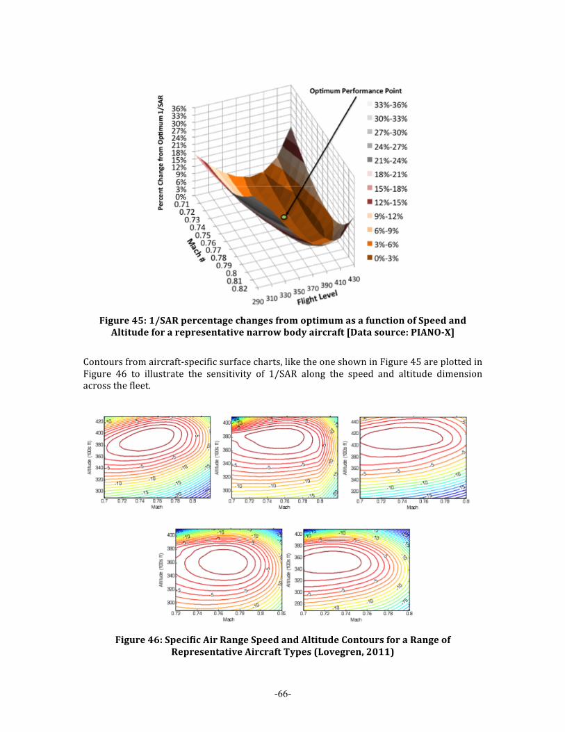
-66-
Figure 45: 1/SAR percentage changes from optimum as a function of Speed and Altitude for a representative narrow body aircraft [Data source: PIANO-X]
Contours from aircraft-‐specific surface charts, like the one shown in Figure 45 are plotted in Figure 46 to illustrate the sensitivity of 1/SAR along the speed and altitude dimension across the fleet.
Figure 46: Specific Air Range Speed and Altitude Contours for a Range of
Representative Aircraft Types (Lovegren, 2011)
!"#

-67-
Because aerodynamic characteristics and engine performance change with speed, there exists some optimal aircraft speed at which aircraft fuel intensity is optimum. As a result, the 1/SAR value (as well as CO2 emissions per mile travelled) is minimized. This speed is defined as Maximum Range Cruise (MRC) and is also known in the industry as 100% SAR speed.
Figure 47: Example 1/SAR sensitivity as a function of speed (fixed altitude and weight) for representative aircraft for five aircraft types from the following
categories: WB, NB, RJ, TP, BJ. [Data source: PIANO-X]
As shown in Figure 47, speed at 100% SAR varies widely amongst aircraft categories (from approximately Mach 0.4 for turboprops to over Mach 0.8 for wide body jets). Due to this variation, identifying and setting a unique speed at which all aircraft should fly during a certification test would introduce a significant bias in 1/SAR measurements and would favor certain aircraft types. Recognizing the fact that airlines will attempt to operate aircraft at speeds not too distant from optimum (i.e. generally between 100%SAR and 99%SAR), a more reasonable and equitable approach would be to allow manufacturers to certify aircraft at a speed that minimizes the value of 1/SAR. A sensitivity analysis using altitude contours for representative aircraft was also conducted to inform the recommendation on the altitude evaluation condition. For every aircraft type, configuration, and flight conditions (e.g. speed, weight) there exists an altitude at which 1/SAR is minimized (Figure 46).

-68-
Figure 48: Illustrative Example of Aircraft Performance Dependence on Altitude
Across the Fleet [Data source: PIANO-X]
Figure 48 illustrates the principle of a variation in aircraft performance across the fleet based on altitude. Using Piano-‐X, five representative aircraft were flown on an equivalent length mission at a fixed altitude. The fuel burn results were normalized to the lowest mission fuel burn to show each aircraft’s sensitivity to altitude, along with deviations across the fleet. It is clear that aircraft are designed to perform optimally at different altitudes (from ~FL200 to ~FL500). Because of this, and the contours depicted in Figure 46, it is unlikely that a single fleet wide altitude assumption could be defined. Thus, the optimum altitude or altitude profile, like speed, varies amongst aircraft types and categories. As such, the most reasonable and equitable approach would be to allow manufacturers to certify aircraft at an altitude that minimizes the value of the 1/SAR.
6.3 Weight As suggested in Equation 11, aircraft weight at the time of evaluation significantly affects 1/SAR. In order to identify an objective and representative weight point it is necessary to evaluate the weight composition of the aircraft fleet in terms of already certified and/or future certifiable points and analyze the sensitivity of 1/SAR as a function of the evaluation weight.
Climb! Descent!Cruise!
Constant !Altitude!
3000 km!
Increasing fuel burn!from minimum!
!"#
$!"#
%!"#
&!"#
'!"#
(!"#
)!"#
*!"#
+!"#
,!"#
!# $!-!!!# %!-!!!# &!-!!!# '!-!!!# (!-!!!# )!-!!!#
!"#$%&"'()"#'*+,"+-.,/'01$+2"'3456'7
.+.6
)6'
04).-"'8#%,)9"':("",;'
./0123#.&+!4+!!#56!,7#
8*&*4+!!#5$*$79:;<=#
>?:?@?/0#>AB#*!!CA#
D?3E#+#FG0/G3#H'!!#IJK#
J2<L3=0G?M#J#N#56,,7#
!"#
$!"#
%!"#
&!"#
'!"#
(!"#
)!"#
*!"#
+!"#
,!"#
!# $!-!!!# %!-!!!# &!-!!!# '!-!!!# (!-!!!# )!-!!!#
!"#$%&"'()"#'*+,"+-.,/'01$+2"'3456'7
.+.6
)6'
04).-"'8#%,)9"':("",;'
./0123#.&+!4+!!#56!,7#
8*&*4+!!#5$*$79:;<=#
>?:?@?/0#>AB#*!!CA#
D?3E#+#FG0/G3#H'!!#IJK#
J2<L3=0G?M#J#N#56,,7#

-69-
Figure 49: 1/SAR and Aircraft Weight evolution over an Illustrative Mission (R1, MSP)
for a Representative Narrow Body Aircraft [Data source: PIANO-X]
Figure 49 shows a detailed flight profile of a representative narrow body aircraft flying a mission at MSP and R1. Aircraft weight decreases quickly during climb (Figure 49, right) as the aircraft burns fuel at a greater rate to reach cruise altitude. Once at cruise altitude, aircraft weight linearly decreases. As such, 1/SAR decreases linearly with the exception of deviations during short phases of step-‐climbing. This further implies that a 1/SAR varies linearly with aircraft weight, which is indeed the case according to Equation 11. One attractive way to measure aircraft weight is to define the evaluation point at a fixed percentage of already certified Maximum Takeoff Weight (MTOW).
Figure 50: Takeoff Weight Iso-Contours for a Representative Narrow Body Aircraft
(Boeing Airport Planning Guides)

-70-
Percentage of MTOW implies a set of possible payload and range missions, as seen in Figure 50 and Figure 9. Aircraft tend to have widely varying fuel and payload fractions as a percentage of MTOW (Figure 51), mostly due to differences in mission design philosophy (Figure 52). For example, longer haul aircraft tend to carry a higher percentage of their maximum takeoff weight in the form of fuel. Additionally, business jets tend to favor low payload capability for a given range (i.e. increase fuel fraction) whereas commercial aircraft (e.g. narrow body jets and wide body jets) have higher payload (and payload fraction) for the same ranges.
Figure 51: Aircraft weight fractions across aircraft categories [Data source: PIANO-X]
Figure 52: Design philosophy differences: maximum structural payload and R1 range
for aircraft in five categories. [Data source: PIANO-X]
Given the consistent takeoff weights shown in 4.4 Takeoff Weights, a solution to mitigate the differences between the widely varying fuel fractions would be to use a single weight assumption that varies appropriately based on aircraft type. Using already certified parameters, a representative average weight can be defined as (MTOW+MZFW)/2, where MZFW is the aircraft Maximum Zero Fuel Weight. This evaluation weight is equivalent to MZFW+50% of total mission fuel at MSP-‐R1.

-71-
6.4 Potential Considerations with Regard to Single Point Evaluation Schemes
One of the evaluation criteria for a CO2 standard is to correlate with CO2 reductions in day-‐to-‐day operations (10.2 Desired Attributes of Certification Requirement). Airplanes fly a variety of routes (i.e. distances) with diverse loadings over their service lifetime (Chapter 4: Typical Aircraft Operations). Thus, to address this criteria, a metric must be evaluated at a certain condition(s) where it can objectively reflect an improvement or degradation in CO2 emissions over a range of different missions that an airplane being certified is anticipated to perform during real operations. Ideally, a CO2 certification requirement based on 1/SAR would be measured at a single evaluation point to reduce the burden of compliance and limit the complexity of the certification process. However, a single evaluation point may not fully represent short-‐haul flight performance for which taxi and climb are a significantly larger portion of the mission. Further, if aircraft performance is not robust and is highly sensitivity to a flight parameter (e.g. speed) within the typical operational range then a single point evaluation may lead to gaps between certified and real-‐world performance due to off-‐optimal operation. A notional example is shown in Figure 53, where aircraft (1) would score better on a single point evaluation but would have worse operational performance than the more robust aircraft (2).
Figure 53: Notional Depiction of Aircraft Robustness to a Flight Parameter
A potential solution is the development of a multipoint evaluation scheme that reflects performance improvements over a broader range of conditions. The development of a multipoint evaluation scheme may more closely resemble day-‐to-‐day aircraft operations and balance the simplicity of measuring 1/SAR and the complexity of defining a full mission based evaluation option.
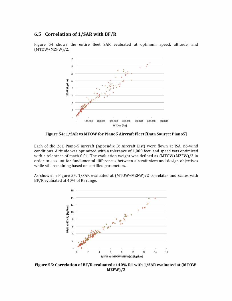
6.5 Correlation of 1/SAR with BF/R Figure 54 shows the entire fleet SAR evaluated at optimum speed, altitude, and (MTOW+MZFW)/2.
Figure 54: 1/SAR vs MTOW for Piano5 Aircraft Fleet [Data Source: Piano5]
Each of the 261 Piano-‐5 aircraft (Appendix B: Aircraft List) were flown at ISA, no-‐wind conditions. Altitude was optimized with a tolerance of 1,000 feet, and speed was optimized with a tolerance of mach 0.01. The evaluation weight was defined as (MTOW+MZFW)/2 in order to account for fundamental differences between aircraft sizes and design objectives while still remaining based on certified parameters. As shown in Figure 55, 1/SAR evaluated at (MTOW+MZFW)/2 correlates and scales with BF/R evaluated at 40% of R1 range.
Figure 55: Correlation of BF/R evaluated at 40% R1 with 1/SAR evaluated at (MTOW-
MZFW)/2
!"!!
!#!!
!$!!
!%!!
!&!!
!'(!!
!'#!!
!'$!!
!'%!!
!"!! !'(()(((!! !#(()(((!! !*(()(((!! !$(()(((!! !+(()(((!! !%(()(((!! !,(()(((!!
!"#$
%&'()"(*
+&
,-./&'&()+&
!"!!
!#!!
!$!!
!%!!
!&!!
!'(!!
!'#!!
!'$!!
!'%!!
(! #! $! %! &! '(! '#! '$! '%!
!"#$%&'%(
)*$ +
%%,-.#-/0%
+#12$%&'%34567849"7:#;%,-.#-/0%
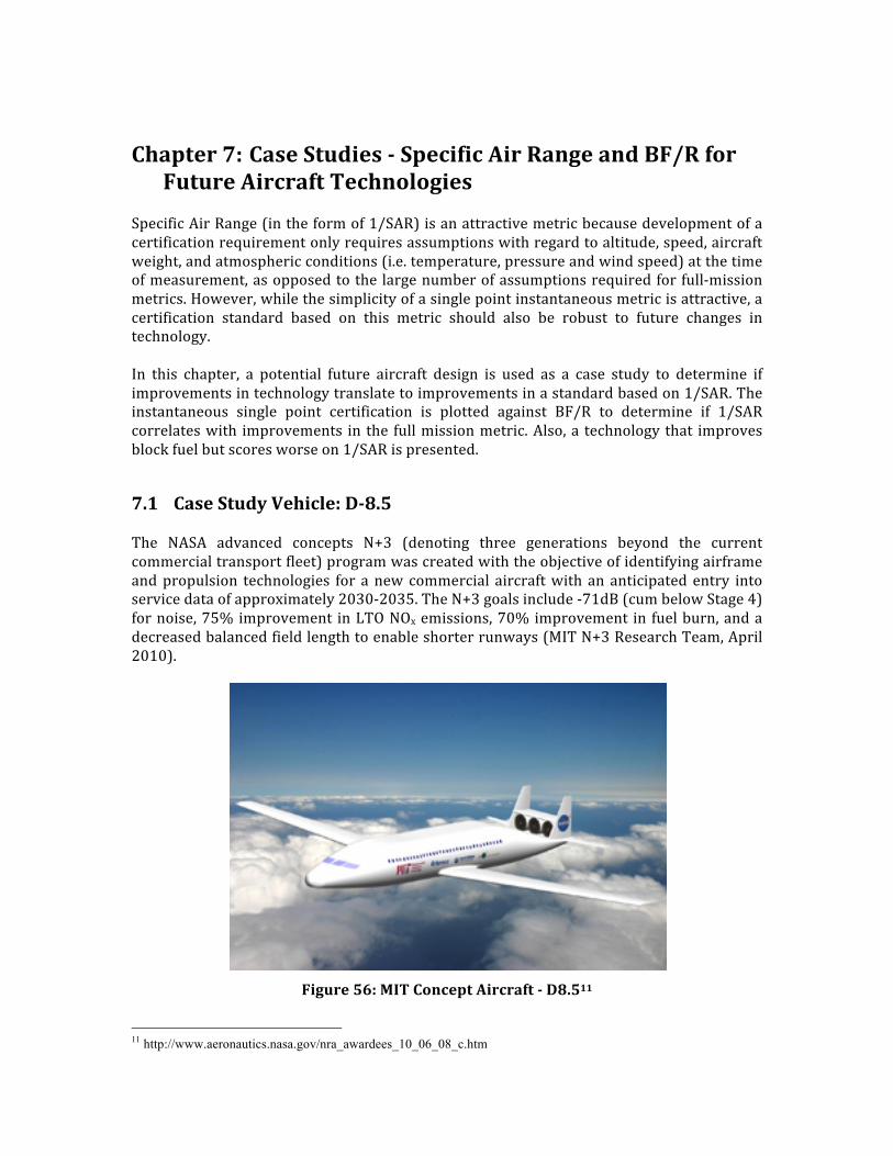
Chapter 7: Case Studies - Specific Air Range and BF/R for Future Aircraft Technologies
Specific Air Range (in the form of 1/SAR) is an attractive metric because development of a certification requirement only requires assumptions with regard to altitude, speed, aircraft weight, and atmospheric conditions (i.e. temperature, pressure and wind speed) at the time of measurement, as opposed to the large number of assumptions required for full-‐mission metrics. However, while the simplicity of a single point instantaneous metric is attractive, a certification standard based on this metric should also be robust to future changes in technology. In this chapter, a potential future aircraft design is used as a case study to determine if improvements in technology translate to improvements in a standard based on 1/SAR. The instantaneous single point certification is plotted against BF/R to determine if 1/SAR correlates with improvements in the full mission metric. Also, a technology that improves block fuel but scores worse on 1/SAR is presented.
7.1 Case Study Vehicle: D-8.5 The NASA advanced concepts N+3 (denoting three generations beyond the current commercial transport fleet) program was created with the objective of identifying airframe and propulsion technologies for a new commercial aircraft with an anticipated entry into service data of approximately 2030-‐2035. The N+3 goals include -‐71dB (cum below Stage 4) for noise, 75% improvement in LTO NOx emissions, 70% improvement in fuel burn, and a decreased balanced field length to enable shorter runways (MIT N+3 Research Team, April 2010).
Figure 56: MIT Concept Aircraft - D8.511
11 http://www.aeronautics.nasa.gov/nra_awardees_10_06_08_c.htm
-74-
MIT developed the D8.5 concept commercial transport aircraft as seen in Figure 56. The D8.5 features a “double bubble” fuselage, lifting body, boundary layer ingestion with high bypass ratio engines, and composite construction, among other technologies. This concept aircraft shows a 60EPNdB noise reduction, 87.3% reduction in LTO NOx, 70.8% reduction in fuel burn, and a reduction of balanced field length to 5,000 feet for metroplex operations (MIT N+3 Research Team, April 2010). The D8.5 was developed by “morphing” a Boeing 737-‐800 through a series of technology introductions and mission specification changes. The mission payload and range, 180 passengers at 215lb per passenger (with luggage) and 3,000nm with 5% fuel reserve, remain the same for all morphing cases. The design objective function is set to minimize fuel burn for all morphing cases.
• Case 0: Baseline Boeing 737-‐800 • Case 1: Boeing 737-‐800 optimized to minimize fuel burn • Case 2: Boeing 737-‐800 fuselage replaced by double bubble fuselage • Case 3: Cruise mach number reduced to 0.76 and aircraft was reoptimized • Case 4: Cruise mach number reduced to 0.72 and the aircraft was reoptimized • Case 5: The CFM56-‐ class engines were moved from the wing to the tail and
mounted flush with the top fuselage. The tail is changed to a pi-‐tail shape. • Case 6: The engine overall pressure ratio was increased from 30 to 35 and the fan,
compressor, and turbine efficiencies were increased one point to reflect 15 years of improved technology relative to CFM56
• Case 7: Slats were removed • Case 8: Balanced field length reduced from 8,000 feet to 5,000 feet • Case 9: Engine technology improved to 2035 timeframe. The bypass ratio was
increased to 20. The metal temperature of the hot section as well as the film cooling effectiveness was increased to 1500 K and 0.4 respectively to allow for a reduction of the required cooling flows. The engine component efficiencies were increased. Advanced engine materials including ceramic matrix composites and titanium aluminum alloys were included, giving rise to a 10% engine weight reduction.
• Case 10: Advanced materials such as carbon fiber reinforced polymer and short carbon nanotubes were used. Also, a reduction of secondary structural weight was included.
• Case 11: Natural laminar flow was considered for 60% of the bottom surface of the wing.
• Case 12: Load reduction technologies such as gust load alleviation, health monitoring, flight envelope protection, and predicting path planning were included on the aircraft design to lower the loading while still operating safely throughout the life of the vehicle.
The D8.5 is a realistic example of future aircraft technology and mission specification changes. For this reason, it will serve as a case study to understand how instantaneous and mission based metrics would measure the fuel efficiency performance at each stage in the morphing analysis12.
12 D8.5 performance data and morphing case descriptions supplied by Dr. Elena de la Rosa Blanco, MIT.

-75-
7.2 Impacts of Measurement on Future Aircraft Designs D8.5 fuel efficiency performance values, 1/SAR at top of climb and overall block fuel at the design range (3,000km), were used to assess the impact of new technology on fuel efficiency performance measurements.
Figure 57: Percent Improvements in 1/SAR and BF/R for Aircraft in MIT D8.5
Morphing Study
Figure 57 shows percent improvements from the baseline aircraft for 1/SAR and BF/R. As can be seen in the figure, the improvements do not exactly scale with one another, but the trend of improvements is nearly identical. This indicates that improvements in a mission metric are also realized as improvements in an instantaneous metric. Likewise, cases that resulted in a negative fuel efficiency performance difference (e.g. case 8 – reducing balanced field length) in BF/R also resulted in a negative performance difference on 1/SAR.
Figure 58: Percent Improvements from Baseline in BF/R vs 1/SAR
!"#
$!"#
%!"#
&!"#
'!"#
(!"#
)!"#
*!"#
+!"#
!# %# '# )# +# $!# $%#
!"#$
%&'()$
)*+",
&'$"-./)01*)"
2'&%31*4"5./)"
6789:"
-,7:"
!"#
$!"#
%!"#
&!"#
'!"#
(!"#
)!"#
*!"#
+!"#
!"# $!"# %!"# &!"# '!"# (!"# )!"# *!"# +!"#
!"#$
%&'()$
)*+",*"-./0"1&'$
"-23)4,*)"
!"#$%&'()$)*+",*"5/670"1&'$"-23)4,*)"
!"
#"$"
%"
&"'"("
)"
*"!+"!!"
!#"

-76-
Figure 58 explicitly shows this trend. Points lying on the 45 degree dashed line show an equivalently scaled percent improvement from the baseline in both the BF/R metrics and the 1/SAR metric. This case study indicates that improvements to a single evaluation point during certification would translate to overall improvements during operations and vice versa. However, consideration should be given towards the fact that while 1/SAR improvements trend with BF/R, a standard comprised of 1/SAR might not equally reward a technology with the same regulatory margin benefit as a BF/R metric.

Chapter 8: Conclusions A fuel efficiency certification standard is one way to reduce aircraft CO2 emissions and mitigate aviation impacts on the climate. In order to develop a commercial aircraft certification standard, a fuel efficiency performance metric and the condition at which it is evaluated was determined. The fuel efficiency metric form identified in this research was fuel/range, where fuel and range can either be evaluated over the course of a reference mission or at a single, instantaneous point. A mission-‐based metric encompasses all phases of flight and is robust to changes in technology; however, definition of the reference mission requires many assumptions and is cumbersome for both manufacturers and regulators. An instantaneous metric based on fundamental aircraft parameters measures the fuel efficiency performance of the aircraft at a single point, greatly reducing the complexity of the standard and certification process; however, a single point might not be robust to future changes in aircraft technology. Typical aircraft operations were assessed in order to develop evaluation assumptions for a mission-‐based metric, Block Fuel divided by Range (BF/R), and an instantaneous metric, incremental fuel burn per incremental distance (inverse Specific Air Range (1/SAR)). Operating patterns and fuel burn maps were used to demonstrate the importance of mission range on fleet fuel burn, and thus the importance of a properly defined range evaluation condition for BF/R. An evaluation condition of 40% of R1 range was determined to be appropriate for the mission-‐based metric. A potential evaluation condition for 1/SAR was determined to be optimal speed and altitude for a representative mid-‐cruise weight defined by half of Maximum Takeoff Weight (MTOW) less Maximum Zero Fuel Weight (MZFW). Good correlation between 1/SAR at (MTOW+MZFW)/2 and BF/R at 40% R1 was shown for the current fleet. A case study of potential future aircraft technologies was presented to show the correlation of improvements in the 1/SAR metric with improvements in BF/R. This demonstrates the suitability of 1/SAR as a potential surrogate for mission-‐based metrics.

-78-
[Page Intentionally Left Blank]

-79-
Chapter 9: Bibliography Air Transport Association of America. (2009). Quarterly Cost Index: U.S. Passenger Airlines. Retrieved 2009 йил September from available at: http://www.airlines.org/economics/finance/Cost+Index.htm B. J. (December 2007). ICAO Committee on Aviation Environmental Protection (CAEP) and Background on Annex 16 to the Chicago Convention. Euromed Aviation Project Safety/Environmental Seminar, Cologne. B. P. (September 2010). Operational Implications of Cruise Speed Reductions for Next Generation Fuel Efficient Subsonic Aircraft. Proceedings of the 27th International Congress of the Aeronautical Sciences, Nice France. Bonnefoy, P. A. (2010). Operation Implications of Cruise Speed Reductions for Next Generation Fuel Efficient Subsonic Aircraft. MIT, Department of Aeronautics and Astronautics. International Congress of the Aeronautical Sciences. Bonnefoy, Y. M. (2011). Assessment of CO2 Emission Metrics for a Commercial Aircraft Certification Requirement. PARTNER. D. D. (1970). 747 Flight Test Certification. Society of Automotive Engineers. D. g. (n.d.). General Information on the NoisedB database. From http://noisedb.stac.aviation-civile.gouv.fr/ F. M. (2004). Initial Flight Testing of the HondaJet. Proceedings of the 24th International Congress of the Aeronautical Sciences, Yokohama, Japan. FAA/MIT (PARTNER). (September 2010). Project 30 Evaluation Options to Support Specific Air Range Metric Recommendation. MIT. Geneva: International Civil Aviation Organization. FAA/PARTNER. (September 2010). Project 30 Metric Recommendation. Geneva: International Civil Aviation Organization. GIACC/4-IP/12. (May 2009). U.S. Fuel Trends Analysis. Presented at the Fourth Meeting of the Group on International Aviation and Climate Change (GIACC/4). Green, J. E. (August 2006). Kuchemann's weight model as applied in the first Greener by Design Technology Sub Group Report: a correction, adaptation and commentary. Aircraft Research Association. The Aeronautical Journal. I. C. (n.d.). Engine Databank. From http://www.caa.co.uk/default.aspx?catid=702&pagetype=90 ICCAIA. (Sept 2010). Considerations for the definition of "Mission Fuel" parameter for evaluation options and fuel efficiency metric puropses. CAEP Working Group 3 CO2TG. Geneva. ICCAIA. (2010). Designing Aeroplanes to Meet a CO2 Standard: A Manufacturers' Perspective. ICAO CAEP/9 Working Group 3 - CO2 Task Group, Second Meeting. ICCAIA. (2010). Overview of concepts associated with the definition of Block Fuel. ICAO CAEP/9 Working Group 3 - CO2 Task Group, Second Meeting. Florence, Italy. International Civil Aviation Organization, C. o. (April, 2009). Consideration of CO2 Standards for Aircraft Engines. London, England: Working Group 3 - Emissions Technical. James K.D. Morrison, B. M. (2011). Transitioning the US Air Transportation System to Higher Fuel Costs. MIT, Department of Aeronautics and Astronautics. K. P. (November 1998). Cycle-Beating and the EU Test Cycle for Cars. Brussels, Belgium. Kirby M., e. a. (September 2010). An Investigation Of The Potential Implications Of A CO2 Emission Metric On Future Aircraft Designs. Proceedings of the 27th International Congress of the Aeronautical Sciences, Nice France. Kirby M., M. D. (September 2008). The Environmental Design Space. Proceedings of the 26th International Congress of the Aeronautical Sciences, Anchorage Alaska. L. D. (2009). Aviation and global climate change in the 21st century. Elsevier.

-80-
L. D. (2003). EC-NEPAIR: Work Package 1, Aircraft Engine Emissions Certification – A Review of the Dof ICAO Annex 16, Volume II. QinetiQ. L. L. (2010). Piano-5. information available at www.piano.aero . used under license: U.S. DOT Volpe Center. L. L. (2010). Piano-5. information available at www.piano.aero . used under license: U.S. DOT Volpe Center. L. L. (2008). Piano-X. information available at www.piano.aero . used under MIT License. Lovegren, J. A. (2011). Estimation of Potential Aircraft Fuel Burn Reduction in Cruise via Speed and Altitude Optimization Strategies. Thesis, Massachusetts Institute of Technology, Aeronautics and Astronautics, Cambridge. M. R. (1936). The Unanticipated Consequences of Purposive Social Action. American Sociological Review. MIT N+3 Research Team. (April 2010). NASA N+3 Final Review. MIT. Langley, VA: NASA. MODTF Rapporteurs. (2008). Implementation of the Fuel Efficiency Metric in GHG Models in Support of Environmental Goals. ICAO Committee on Aviation Environmental Protection Modeling and Task Force Meeting. Sixth Meeting. Miami: CAEP/8 MODTF. N. G. (February 2010). Boeing Details 747-8 Freighter Flight Test Plan. National Research Council, T. R. (2002). Effectiveness and Impact of Corporate Average Fuel Economy (CAFE) Standards. Washington D.C.: National Academies Press. Raymer, D. P. (2006). Aircraft Design: A Conceptual Approach (Fourth Edition ed.). Reston, VA: AIAA. Regulatory Announcement: New Emission Standards for New Commercial Aircraft Engines EPA420-F-05-015. (2005 йил November). From http://www.epa.gov/oms/regs/nonroad/aviation/420f05015.htm S. S. (2007). Climate Change 2007: The Physical Science Basis. Contribution of Working Group I to the Fourth Assessment Report of the Intergovernmental Panel on Climate Change. NY: Cambridge University Press. SEC. (1999 йил 19-3). SEC Info - US Airways Group Inc, et. al. Retrieved 2011 йил May from SEC Info: http://www.secinfo.com/dWcTe.67.b.htm?Find=PERFORMANCE%20GUARANTEES#1stPage U. E. (April 2010). Inventory of U.S. Greenhouse Gas Emissions and Sinks: 1990-2008. U.S. Department of Transportation, B. o. (n.d.). From http://www.transtats.bts.gov/databases.asp?Mode_ID=1&Mode_Desc=Aviation&Subject_ID2=0 U.S. Department of Transportation, F. A. (November 1969). Adoption of Noise Type Certification Standards and Procedures. U.S. Department of Transportation, V. C. (2006). Common Operations Database. W. D. (2006). Workshop on the Impacts of Aviation on Climate Change: A Report of Findings and Recommendations. Cambridge, MA. W. D. (August 2006). Workshop on the Impacts of Aviation on Climate Change: A Report of Findings and Recommendations. Cambridge, MA.

Chapter 10: Appendix
10.1 Appendix A: Background Review of Aviation and Non-Aviation Certification Standards13
10.1.1 NOx The NOX emission standards were established on the recommendation of CAEP/2. The CAEP/2 standard was adopted by ICAO member states with few, if any, exceptions as the universally recognized international standard for aviation. It is to be applied to all engines produced after 2000, to all new and derivative engines for which certification has been or is to be applied for after 1995, and, as a practical matter, to currently certified in-‐production engines that are to be altered to meet the standard.
Figure 59: NOx performance metric, correlating parameter, and regulatory levels
(Bonnefoy Y. M., 2011)
10.1.1.1 Metric The metric used to regulate aircraft engine emissions (Figure 59) is DP/F00, where DP is the mass of pollutants emitted and F00 is the engine’s sea level static maximum rated thrust. This metric was chosen in part because it succinctly relates emissions performance to the useful capability of the engine.
13 This section originally appeared in greater detail in REPORT NO. PARTNER-COE-2011-002 (Bonnefoy, Y. M. (2011). Assessment of CO2 Emission Metrics for a Commercial Aircraft Certification Requirement. PARTNER.), and was the collaborative effort of all authors.
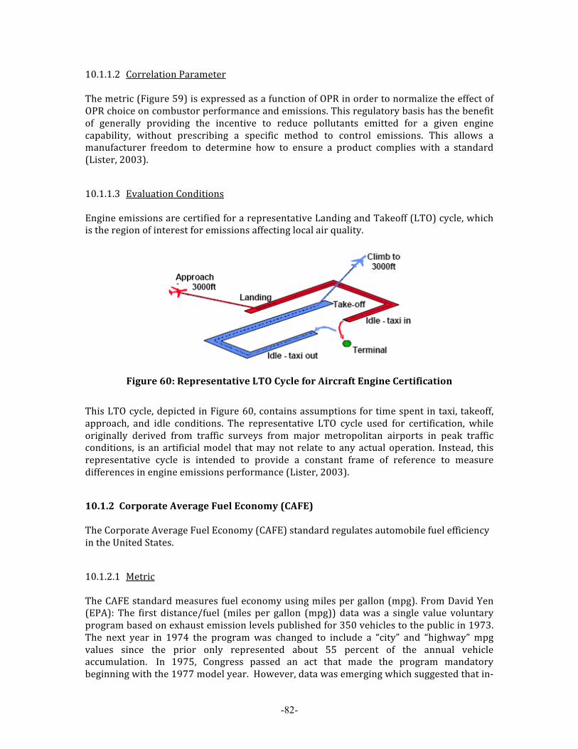
-82-
10.1.1.2 Correlation Parameter The metric (Figure 59) is expressed as a function of OPR in order to normalize the effect of OPR choice on combustor performance and emissions. This regulatory basis has the benefit of generally providing the incentive to reduce pollutants emitted for a given engine capability, without prescribing a specific method to control emissions. This allows a manufacturer freedom to determine how to ensure a product complies with a standard (Lister, 2003).
10.1.1.3 Evaluation Conditions Engine emissions are certified for a representative Landing and Takeoff (LTO) cycle, which is the region of interest for emissions affecting local air quality.
Figure 60: Representative LTO Cycle for Aircraft Engine Certification
This LTO cycle, depicted in Figure 60, contains assumptions for time spent in taxi, takeoff, approach, and idle conditions. The representative LTO cycle used for certification, while originally derived from traffic surveys from major metropolitan airports in peak traffic conditions, is an artificial model that may not relate to any actual operation. Instead, this representative cycle is intended to provide a constant frame of reference to measure differences in engine emissions performance (Lister, 2003).
10.1.2 Corporate Average Fuel Economy (CAFE) The Corporate Average Fuel Economy (CAFE) standard regulates automobile fuel efficiency in the United States.
10.1.2.1 Metric The CAFE standard measures fuel economy using miles per gallon (mpg). From David Yen (EPA): The first distance/fuel (miles per gallon (mpg)) data was a single value voluntary program based on exhaust emission levels published for 350 vehicles to the public in 1973. The next year in 1974 the program was changed to include a “city” and “highway” mpg values since the prior only represented about 55 percent of the annual vehicle accumulation. In 1975, Congress passed an act that made the program mandatory beginning with the 1977 model year. However, data was emerging which suggested that in-‐
-83-
use passenger vehicles were not achieving the fuel economy levels listed on the labels and in the Guides. Citizen complaints, Congressional subcommittee hearings, and law suites resulted in the 1979 model year vehicles only having a “city” value being used for overall driving while the EPA began an in-‐depth study to develop a solution. In 1985 after test adjustments to deal with the in-‐use shortfall, an addition of “highway” mpg was added to the labels again. In the early 2000’s renewed concerns over in-‐use shortfall of label values similar to those that drove the 1979 model year changes developed. In 2008, EPA began a revised label calculation method to account for in-‐use shortfalls based on 5 test cycles(City(FTP), Highway (HFET), High Speed & Aggressive Drive (US06), Air Conditioning Test (SC03), 20 degree Fahrenheit Drive Mode (FTP)) that now account directly for factors such as air conditioning, aggressive driving, high speed cruise, and cold temperatures. “City” and “Highway” values are still listed on the new light weight vehicle labels. The general public expects accuracy and representativeness based on how the vehicle is operated in actual operational patterns. Today mileage/fuel is not a characteristic of the vehicle with some SUVs getting 34 mpg city, and some passenger cars that achieve 14 mpg city; they are a characteristic of technology, operations, and other factors.
10.1.2.2 Correlating Parameter Through 2011, passenger car and light trucks were subject to standards based solely on mpg. However, beginning in 2008 and subject to the choice of the manufacturer, optional reformed standards were applied that imposes standards for light trucks based on the same fuel economy metric but also expressed as a function of vehicle footprint. This change was motivated by the findings of a National Academy of Sciences report evaluating the effectiveness of the CAFE standards, which found the CAFE program “might be improved significantly by converting it to a system in which fuel targets depend on vehicle attributes (National Research Council, 2002).” These reformed light truck standards are currently in a transition period through 2011, when all light trucks will be required to comply with this reformed standard based on this vehicle attribute. Furthermore, it has been proposed that similar attribute-‐based standards be extended to passenger cars beginning in 2011.
10.1.2.3 Evaluation Conditions The measurement of vehicle fuel efficiency within the CAFE standard is achieved with the use of a set of test cycles. Various parameters such as engine run-‐in time before testing, track conditions, maximum speed, repeatability of results, and weather conditions are all prescribed by the respective governing bodies. These conditions are meant to create consistent results across many different manufacturers. While a test cycle cannot possibly exactly reproduce the driving conditions of every type of driver, the test cycles intend to mimic normal driving conditions the vehicle will typically operate at during its lifetime. Evidence has been presented that manufacturers have participated in “cycle beating:” developing their cars and engines to perform better on the test cycle than they would in day-‐to-‐day operations. It is clear that choosing a test cycle that accurately represents the way the vehicle will be operated is very important for a robust emission metric. Without this appropriate test cycle, there is the possibility for manufacturers to participate in cycle beating or other methods of gaming the system (Kageson, November 1998).

-84-
10.1.2.4 Scope of Applicability This standard applies to manufacturer’s fleet of any model year passenger cars or light trucks with a gross vehicle weight rating (GVWR) of 8,500 lbs. or less and manufactured for sale within the United States. Fuel economy is defined as the average mileage traveled by an automobile per gallon of gasoline (or equivalent amount of other fuel) consumed as measured in accordance with the testing and evaluation protocol set forth by the EPA. The current CAFE limit on light vehicles is 27.5 mpg with a financial penalty for companies with a fleet average above this value. The penalty is $5.50 per tenth of a mpg under the target value, per vehicle sold by the company.
10.2 Desired Attributes of Certification Requirement The first steps in creating a list of desired attributes of a certification requirement were literature review, brainstorming, and interactions with stakeholders. Collective engineering judgment was used to generate the following desired attributes of a certification requirement. They closely mimic the “key criteria” of the CO2TG (IP27).
Differentiate generations of CO2 reduction technologies. A metric and CP system should clearly distinguish between levels of inherent aircraft technology levels, so as to best encourage the introduction of fuel efficient technologies in the future
Exhibit independence of purpose or utilization. A metric and CP system should not discriminate between the performance of aircraft intended for different purposes in use.
Account for fundamental airplane design elements and capabilities. Not require inappropriate amount of resources to implement. The parameters
in the metric, CP, and evaluation option should limit the burden on the authorities to implement as part of a certification requirement.
Explainable to the general public. The parameters in the metric and CP should be simple and easily understood by the layman.
Be easily measurable. The metric should be based upon certified parameters to ensure commonality between different manufacturers. The parameters that compose the metric should be easily measurable at the certification stage, or derived from engineering data, and should consider the industry certification requirement practices of measurement and adjustment. In order to ensure the successful implementation of a CO2 certification requirement, there is a need to limit the regulatory burden associated with obtaining and tracking information to a reasonable level,
Be fair (equitable) across set of stakeholders. To the extent practicable, the metric should be fair across the set of stakeholders covered by the CO2 certification requirement, including the distribution of cost and benefits, when initially applied and with respect to the future,
Limit unintended consequences. The use of poorly defined metrics to establish policies can create equity issues and can result in the emergence of opportunities to influence the system in a way that may reduce the effectiveness of the policies and have the potential to drive the system to a different operating point than the one originally intended,

-85-
Be based on evaluation conditions that are representative of typical aircraft operations. In order to avoid single point performance optimization and limit gaming dynamics, the metric should be computed at “evaluation points” that are representative of typical aircraft operations,
Maximize the environmental benefit. The metric (when adopted as part of a certification requirement) should contribute to achieving the highest effectiveness at reducing CO2 emissions both at the vehicle-‐level and at a system-‐wide aggregate level.
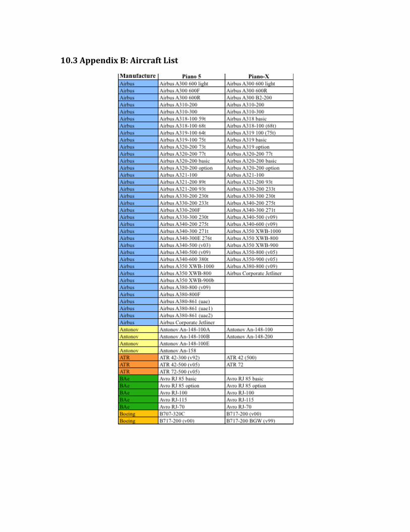
10.3 Appendix B: Aircraft List

-87-

-88-
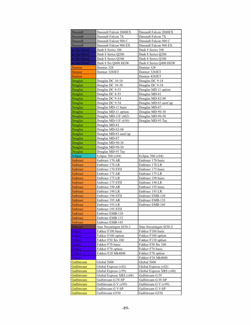
-89-

-90-