APPROACHES TO OPEN QUANTUM SYSTEMS: DECOHERENCE ...
113
APPROACHES TO OPEN QUANTUM SYSTEMS: DECOHERENCE, LOCALISATION AND ALL THAT by Ting Yu Department of Physics Imperial College of Science, Technology and Medicine Submitted in partial fulfilment of the requirements for the degree of Doctor of Philosophy at the University of London and for the Diploma of Membership of Imperial College March 1998
Transcript of APPROACHES TO OPEN QUANTUM SYSTEMS: DECOHERENCE ...
APPROACHES TO OPEN QUANTUM SYSTEMS: DECOHERENCE,
LOCALISATION AND ALL THAT
by
Ting Yu
Department of Physics
Imperial College
of Science, Technology and Medicine
Submitted in partial fulfilment of the requirements for the degree of
Doctor of Philosophy at the University of London
and for the Diploma of Membership of Imperial College
March 1998
A b s t r a c t
This thesis is mainly concerned with issues in quantum open systems
and the foundations of quantum theory.
Chapter I introduces the aim, background and main results which
take place in the following chapters. Chapters II and III are used to
study and compare the decoherent histories approach, the environment-
induced decoherence and the localisation properties of the solutions to
the stochastic Schrodinger equation in quantum jump simulation and
quantum state diffusion approaches, for a quantum two-level system
model. We show, in particular, that there is a close connection between
the decoherent histories and the quantum jump simulation, comple-
menting a connection with the quantum state diffusion approach noted
earlier by Diosi, Gisin, H alii well and Percival. In the case of the de-
coherent histories analysis, the degree of approximate decoherence is
discussed in detail. As by-product, by using the von Neumann entropy,
we also discuss the predictability and its relation to the upper bounds
of degree of decoherence.
In Chapter IV, we give an alternative and elementary derivation of
the Hu-Paz-Zhang master equation for quantum Brownian motion in
a general environment, which involves tracing the evolution equation
for the Wigner function. We also discuss the master equation in some
special cases. This master equation provides a very useful tool to study
the decoherence of a quantum system due to the interaction with its
environment.
In Chapter V, a derivation of the parameter-based uncertainty re-
lation between position and momentum is given. This uncertainty
relation can be regarded as an exact counterpart of the time-energy
uncertainty relation.
The final chapter is a rather brief summary of the thesis.
Decla ra t ion
The work in this thesis was carried out in the Theoretical Physics
Group, Imperial College, London between October 1994 and October
1997 under the supervision of Dr. J. J. Halliwell.
The thesis is based on a series of published papers [Physical Review,
D 53, 2012 (1996); Physics Letters, A 223, 9 (1996) and Physica, A
248, 393 (1998)]. In particular. Chapter four in the thesis is based on a
collaboration work with Jonathan Halliwell. I would like to thank him
for his kind permission to include it into this thesis.
The work presented in this thesis, except where otherwise stated, is
original and has not been submitted before for any degree or diploma
of this or any other university.
4
Acknowledgements
First and foremost, I would like to thank my supervisor Jonathan Halli-
well for his insightful advice, constant encouragement and great support
in the various stages of my PhD studies. I thank him for bringing me
into a wonderful new research field - Decoherence and Quantum Open
System, which is full of exciting ideas and adventures. I would also like
to thank the other members of Theory Group for their various help and
support.
I have benefited over last three years from many people through
conversations, correspondences and lectures, I would like here to thank
all of them. In particular, I am very grateful to Lajos Diosi, Bei-Lok liu
and Ian Percival for very useful discussion and encouragement. I am
also grateful to Charalambos Anastopoulos, Dorje Brody, Todd Brun,
Bernhard Meister, Zhaoyan Wu and Andreas Zoupas for discussions
and communications.
To my two sisters, Shuqin Yu and Jianhua Yu, I owe a special thank.
Over years they have given me their enormous selfless support.
I would like to thank my wife Jingshi and my daughter Linda for
their understanding, support and love.
Finally, the financial support from the British Council through
SBFSS fellowship is gratefully acknowledged.
To
the memory of my mother, Guofeng Han-Yu
and to
my father, Tian-Cai Yu
Contents
1 Introduction 8
2 Decoherence and Predictability 14
2.1 Environment-induced decoherence 15
2.2 Decoherent histories approach 17
2.3 Two-state model 21
2.4 Decoherent histories in the two-level system m o d e l . . . . 27
2.4.1 Decoherent history analysis 27
2.4.2 Decoherent history vs. environment-induced de-
coherence 31
2.5 Degree of decoherence and predictability 33
2.5.1 Approximate decoherence 33
2.5.2 von Neumann entropy and predictability 40
2.6 Discussion 43
3 Stochastic Localisation Processes 46
6
CONTENTS 7
3.1 Unravelling of master equation 46
3.1.1 Quantum jump simulation 47
3.1.2 Quantum state diffusion 52
3.2 Discussion 60
4 Quantum Brownian motion 63
4.1 Introduction 64
4.2 Master equation for quantum Brownian motion 65
4.3 Determination of coefficients (general case) 72
4.4 Particular cases 81
4.5 Discussion 84
5 Parameter-based Uncertainty Relations 86
5.1 Introduction 86
5.2 Derivation of uncertainty relation 88
5.3 Summary 92
6 General Conclusion 94
A Proof of theorem 96
B Coefficients in master equation of Q B M 99
Chapter 1
Introduction
"What sort of things do you re-member best?" Alice ventured to ask. "Oh, things that happened the week after next," the Queen replied in a careless tone.
—Lewis Carroll Through the Looking-Glass
Quantum theory has been so successful that it has been regarded as
a universal physical theory. On the one hand, it allows precise calcula-
tion of various physical processes and the theoretical calculations agree
with empirical data to a remarkable degree. On the other hand, the
foundation of quantum theory, at least the Copenhagen interpretation,
has made many physicists uneasy even since the birth of the theory.
In the Copenhagen interpretation [1], the measuring devices or clas-
sical observers play an integral part in the formulation of the theory.
Quantum theory takes classical theory as its limiting case while as an
indispensable part of its own theoretical formulation.
Moreover, the measurement problem in quantum theory has never
been fully settled. The von Neumann projection postulate is only an
ad hoc hypothesis which is imperfectly understood. The measurement
process is not described by the Schrodinger equation. One can only
talk about the measured results, but not the measuring process itself.
In quantum cosmology, the situation is even worse. Quantum theory
of the whole universe must be interpreted without relying on the so-
called classical outside observer.
In summary, the traditional Copenhagen interpretation is inade-
quate, since it relies on an outside classical domain.
In last three decades, several proposals have been made to over-
come the weak points of the Copenhagen interpretation. A real break-
through has occurred in recent years. Two primary paradigms - the
environment-induced decoherence approach, proposed by Zurek [2, 3,
4], and the consistent histories approach by Griffiths [5] and later by
Omnes [6, 7] and by Gell-Mann and Hartle [8, 9, 10] have been recently
developed to solve the fundamental issues in quantum theory, especially,
quantum measurement problems and the transition from quantum to
classical. The environment-induced decoherence emphasises the divi-
sion between the system and its environment. The interaction of the
10 CHAPTER 1. INTRODUCTION
system with its environment is responsible for the decay of the quantum
coherence of the system. The decoherent histories approach is designed
to provide the most general descriptions for a closed system by using
the concept of history - a sequence of events at a succession of times.
Both approaches are appHcable to open quantum systems.
Another set of viable theories within the framework of quantum
mechanics are the various unravellings of master equation as stochastic
Schrodinger equations for the single member of the ensemble. Among
others, the quantum state diffusion by Gisin and Percival and the quan-
tum jump simulation approaches have been extensively studied in re-
cent years {e.g., see [11, 12, 13, 14, 15]). As phenomenological theories,
these stochastic approaches are not only of theoretical interest but also
of practical value.
The open quantum system provides a unified framework to exhibit
the properties of the various approaches we have mentioned above. The
master equation which describes the evolution of the open quantum sys-
tem plays a central role in the investigations into the decay of quantum
coherence due to the interaction with a much larger environment. It
does not, however, tell us how an individual member of an ensemble
evolves in a dissipative environment. The unravelling of master equa-
tion as stochastic Schrodinger equation could provide such a description
11
within its domain of applicability. Corresponding to the decoherence
process in the density operator formalism, in stochastic Schrodinger
equation approaches, the solution to the stochastic Schrodinger equa-
tion often possesses a very remarkable property - the solution tends
to localise at some special states after a localisation time scale. For
quantum state diffusion approach, this localisation property has been
justified in many different situations [14, 15, 16, 17, 18, 19].
It is worth emphasising that a key point in these approaches is the
mutual influence between the system of interest and its environment.
This mutual influence is the common sources of the many different
phenomena such as dissipation, fluctuation, decoherence, localisation,
etc.
Analysis of decoherence and localisation properties is usually rather
involved. The entanglement of the complicated mathematics and the
subtle conceptual issues often tends to make detailed scrutiny of the
basic concepts impossible. The some quantum optical models and quan-
tum Brownian motion models, as exactly solvable models, are of great
attractiveness due to their simplicity and yet physical meaningfulness.
The purposes of this thesis are following: First, in Chapters II and
III, we will employ a widely used quantum open system model — a two
level system model as a unified framework to examine the dynamics of
12 CHAPTER 1. INTRODUCTION
the open quantum system by decoherent histories, environment-induced
decoherence and stochastic Schrodinger equations. We mainly consider
the decoherence process and the localisation process. The various time
scales concerning these processes are discussed. One of main result in
this part is an establishment of a close connection between the deco-
herence histories and quantum jump simulation [20], complementing a
connection with quantum state diffusion noted earlier by Diosi, Gisin,
H alii well and Percival [18]. By using this simple model, we have com-
pared the decoherent histories and environment-induced decoherence
approaches in some detail. In the case of the approximate decoher-
ence, we provide a detailed analysis of the degree of decoherence of the
two-level models, which is important for a real physical process.
Second, we provide, in Chapter IV, an alternative derivation of mas-
ter equation for quantum Brownian motion model in general environ-
ment at arbitrary temperature [21]. This is another typical quantum
open system model. Our derivation is physically natural and mathe-
matical simple.
Finally, in Chapter V, we present a derivation of a new uncertainty
relation between position and momentum which can be served as a
counterpart of the time-energy uncertainty relation [22].
The plan of this thesis is as follows. In Chapter I, we present a
13
brief introduction of conceptual development of our research subjects.
In Chapter II, after a brief review of environment-induced decoher-
ence and decoherent histories approaches, we present a two-level system
model and its basic properties. We then study the consistent histories
approach and its relation to the environment-induced decoherence, the
degree of decoherence and predictability by using von Neumann en-
tropy. In Chapter III, we study the unravelling of master equation and
the localisation properties of the solutions to the stochastic Schrodinger
equations in both quantum jump simulations and quantum state diffu-
sions. We discuss the quantum Brownian motion and parameter-based
uncertainty relation in Chapters IV and V, respectively. We finally
conclude the whole thesis in Chapter VI. The proof of a Theorem in
Chapter II and an alternative determination of coefficient of master
equation of QBM in Chapter V are included in the appendices.
Chapter 2
Decoherence and Predictability
"All right" said the Cat; and this time it vanished quite slowly, be-ginning with the end of the tail, and ending with the grin, which remained some time after the rest of it had gone.
—Lewis Carroll Alice's Adventures in Wonderland
The first purpose of this chapter is to examine, by making use of a
two-level system, the two rival approaches: environment-induced deco-
herence and decoherent histories approaches. In particular, the deco-
herent histories analysis for this two-level model will be used to compare
with quantum jump simulation and quantum state diffusion approaches
in Chapter 3.
Our second purpose is to investigate the degree of approximate de-
coherence by using Dowker-Halliwell criterion. We also show a rela-
14
2.1. ENVIRONMENT-INDUCED DECOHERENCE 15
tionship between the predictability and von Neumann entropy.
This chapter will concentrate on examining the decoherence process
in a two-level system, starting with a brief review of both environment-
induced decoherence and decoherent histories approaches, which play
a central role in the next two chapters.
2.1 E n v i r o n m e n t - i n d u c e d decoherence
Decoherence of density matrices (often called the environment-induced
decoherence) was initiated by Zurek for the purpose of providing a so-
lution to the measurement problem [2]. The essence of this theory is to
single out, through the interaction of the system with its environment,
some special states (often called the pointer basis) which remain least
affected by the interaction of environment.
It has been noticed that macroscopic objects are impossible to iso-
late from their surroundings [23, 24]. The constant interaction of the
system with the large environment results in a decoherence process
(often in a very short time scale) which destroys the all possible super-
positions of macroscopically distinct states [4, 24]. One consequence of
this decoherence, being described by a density matrix, is that, after a
decoherence time scale, the density matrix is approximately diagonal
in the pointer basis.
16 CHAPTER 2. DECOHERENCE AND PREDICTABILITY
In some idealised models [2], the self-Hamiltonian of the system Hg
was completely neglected or was assumed codiagonal with interaction
Hamiltonian Hint- The eigenstates of an observable A which satisfies
[Hs + Hint, A] = 0
naturally constitute a "pointer basis".
In realistic physical processes, however, a set of nontrivial observ-
ables which simultaneously commute with both the self- and interaction
Hamiltonian is not likely to exist. In fact, during the decoherence pro-
cess, all of the states in Hilbert space will be affected by the interaction
with environment, the "pointer basis" are the states that are most sta-
ble, so they can be selected by a "predictability sieve" [4, 25, 26].
We should mention that the emergence of classicality is in a central
position in both environment-induced decoherence and consistent his-
tories programmes. But it is noticeable that the criteria for classicality
are not entirely clear.
It has been argued that the consistent histories approach cannot
provide a complete characterisation of classicality without borrowing
the concepts from the other formalisms such as environment-induced
decoherence [27]. More thorough investigation into this aspect would
be important.
2.2. DECOHERENT HISTORIES APPROACH 17
Based on the quantum Brownian motion model, Zurek et al [26]
have characterised the effectiveness of decoherence in terms of a. pre-
dictability sieve, and identified the maximally predictive states as the
most classical, and have shown that coherent states are maximal. It
seems that entropy plays important role in these studies.
2.2 Decoheren t his tor ies a p p r o a c h
The consistent histories approach was proposed by Griffiths [5] and
developed by Omnes [6, 7] and by Gell-Mann and Hartle [8, 9, 10]. The
reviews of the theory and some important developments can be found
in [28, 29, 30, 31, 32, 33].
A history is defined in general as a sequence of properties of an
isolated system occurring at different times. Precisely, suppose that
system is given at initial time to by a density matrix p and (1,^2,- -
is a sequence of time satisfying
We also suppose that, at each time a property of system, represented
by a projection operator will be assigned. A typical history is denoted
as
18 CHAPTER 2. DECOHERENCE AND PREDICTABILITY
where P^^{ti) are the projection operators in the Heisenberg picture at
times tf.
f (2.1)
here, H is the Hamiltonian of the closed system. These projection
operators satisfy exhaustive and exclusive conditions:
E P S ( t - ) ='' (2.2) CVi
The superscript {i) labels the set of projections used at time ti and a,
denotes the particular alternative.
Like in ordinary probability theory, rather than merely consider-
ing single history, one usually considers the whole sample space which
contains all possible outcomes.
The main goal of decoherent histories approach is to assign each
history a probability without referring to the measurements. A natural
way to assign the probability to a history is
p(C„) = Tr(Ctp(i„)C„)
= (2.3)
However, one finds that (2.3) generally does not satisfy the usual
probability sum rule. Precisely, for two different histories Ca and Cq,/,
one would not expect that
p{Ca + Ca') = p{Ca) + p{Ca')
2.2. DECOHERENT HISTORIES APPROACH 19
always holds.
The necessary and sufficient condition to guarantee the above equa-
tion holds is the real part of decoherence functional D[a,Q/] vanishes.
i.e.:
Re£>[a,^] = ReTr(C^X^o)Ca') = 0 (2.4)
for any two different histories Cq. and Ca'- The sets of histories sat-
isfying (2.4) are said to be consistent (or weakly decoherent). Physi-
cal mechanisms causing (2.4) to be satisfied typically lead also to the
stronger condition
D[a,a']=0, Ma^ol (2.5)
which is called medium decoherence [9]. (In this thesis, we simply refer
it as decoherence)
Decoherent histories approach ofl:ers a sensible way to assign proba-
bility to a sequence of properties of a quantum system without referring
to the measurement. It has many appeaUng features. Some of them
are mentioned as follows:
1. Physically interesting histories are seldom exactly decoherent,
they satisfy, at best, the so-called approximate decoherence conditions
[9,30].
2. Generally, only coarse-graining histories can be consistent. Obvi-
ously, the coarse-graining preserves decoherence but loses information
^For simplicity we write Ca as a .
20 CHAPTER 2. DECOHERENCE AND PREDICTABILITY
about the system (initial state).
3. The existence of decoherent sets of histories is closely related to
the existence of records, i.e. storage of information about the system
of interest somewhere in the environment [9, 28].
4. Although the decoherent histories approach was primarily de-
signed for a closed system, the approach is of particular importance for
a open system which may be regarded as a subsystem of a large closed
system. For the open quantum system, a natural coarse-graining is to
focus only on the properties of the distinguished system whilst ignoring
the environment. In this case, a natural selection of projections at each
time is of form 0 where Pa is a projection onto the distinguished
subsystem and denotes the identity projection on the environment.
In the Markovian regime, the decoherence functional could be con-
structed entirely in terms of the reduced density matrix of the system
[27]:
(2.6)
where the trace is taken over the distinguished system only. The quan-
tity Ktk-il ' ] super-propagator for the reduced density operator:
= Kl[po]. This property will be well used in the following discussions
in this and next chapters.
2.3. TWO-STATE MODEL 21
5. It has been argued that consistent histories approach can be used
to characterise the emergence of classical behaviour from the quantum
substrate, a quasi-classical domain is defined as a set of decohering,
maximally refined coarse-grained histories that exhibit strong correla-
tions according to some deterministic law [8, 9]
6. Finally, we should mention that the decoherent histories ap-
proach is related to another mechanism of transition from quantum to
classical which bear the same name - decoherence proposed by Zurek (a
brief review of this approach is given in last subsection). The relation
between these two approaches have been discussed^ [27, 34, 35, 36].
2.3 Two-s ta t e mode l
A two-level system can be regarded as, in some sense, the fundamen-
tal building block in quantum theory. We consider a two-level atom
system, which is radiatively damped by its interaction with the many
modes of a radiation field in thermal equilibrium at temperature T.
The upper level and lower level are denoted by |2) and |1), respec-
tively. This is a typical example of the so-called system-plus-reservoir
models in which quantum mechanics is fully implemented. In the case
of our model, the system of interest is a single atom, and the reservoir
^We will compare those two approaches based on a two-level systems in Section 2.4.2
22 CHAPTER 2. DECOHERENCE AND PREDICTABILITY
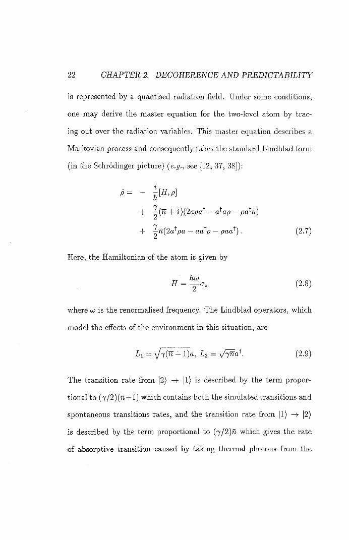
is represented by a quantised radiation field. Under some conditions,
one may derive the master equation for the two-level atom by trac-
ing out over the radiation variables. This master equation describes a
Markovian process and consequently takes the standard Lindblad form
(in the Schrodinger picture) (e.g., see [12, 37, 38]):
+ '^(n + l)(2apa^ — a'^ap — pa'^a)
4- ^n(2a^pa — aa^p — paa^) . (2.7)
Here, the Hamiltonian of the atom is given by
ff = (2.8)
where w is the renormalised frequency. The Lindblad operators, which
model the effects of the environment in this situation, are
Li = 1)«, ^2 = (2.9)
The transition rate from |2) -4 |1) is described by the term propor-
tional to (7/2)(n-l-l) which contains both the simulated transitions and
spontaneous transitions rates, and the transition rate from |1) |2)
is described by the term proportional to (7/2)n which gives the rate
of absorptive transition caused by taking thermal photons from the
2.3. TWO-STATE MODEL 23
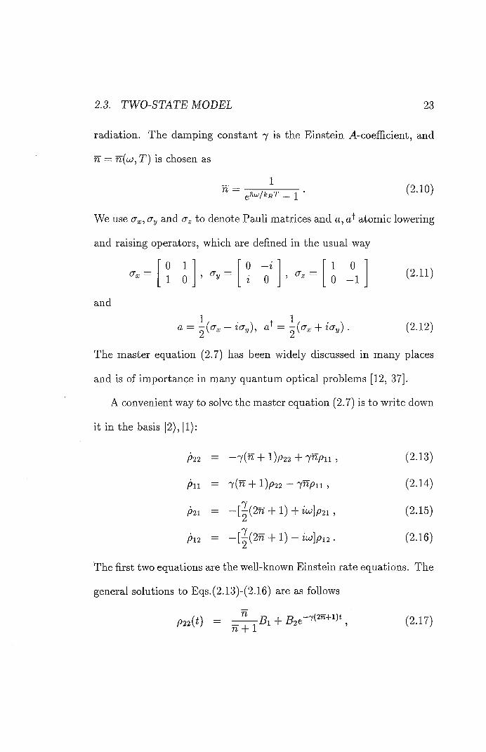
radiation. The damping constant 7 is the Einstein A-coefiicient, and
n = n{(jj, T) is chosen as
" = gRw/kgT _ 1 •
We use <Tr, cTy and cr to denote Pauli matrices and a, atomic lowering
and raising operators, which are defined in the usual way
" 0 1 • ' 0 - i ' • 1 0 —
1 0 , CTy —
I 0 , (Tz =
0 - 1
and
-{(7^ — i(Ty)^ a) — -{(7:^ icTy) .
(2.11)
(2.12)
The master equation (2.7) has been widely discussed in many places
and is of importance in many quantum optical problems [12, 37].
A convenient way to solve the master equation (2.7) is to write down
it in the basis j2), |1):
P22 = - 7 ( " + l ) / ) 2 2 + 7 " P i i ,
Pii = 7 ( " + l)p22 - ^npii ,
P 2 1 r 7 (2n + 1) -(- iio\p2i 1
Pi2 = — [•^(2n-F 1) — ia;]pi2 .
(2.13)
(2.14)
(2.15)
(2.16)
The first two equations are the well-known Einstein rate equations. The
general solutions to Eqs.(2.13)-(2.16) are as follows
(2.17) P22\
24 CHAPTER 2. DECOHERENCE AND PREDICTABILITY
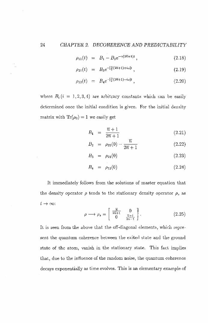
m i W = (2.18)
= B3e-[2(2"+i)+^w]f^
(2.20)
where Bi{i = 1,2,3,4) are arbitrary constants which can be easily
determined once the initial condition is given. For the initial density
matrix with Tr(po) — 1 we easily get
«• = _ P-"' ft
B2 = ^22(0) - (2.22)
B3 = P2i(0) (2.23)
B4 = ^12(0) (2.24)
It immediately follows from the solutions of master equation that
the density operator p tends to the stationary density operator ps as
t - 4 - 0 0 :
r " n 1 (2.25)
2 ^ 0 0
2n+l
It is seen from the above that the off-diagonal elements, which repre-
sent the quantum coherence between the exited state and the ground
state of the atom, vanish in the stationary state. This fact implies
that, due to the influence of the random noise, the quantum coherence
decays exponentially as time evolves. This is an elementary example of
2.3. TWO-STATE MODEL 25
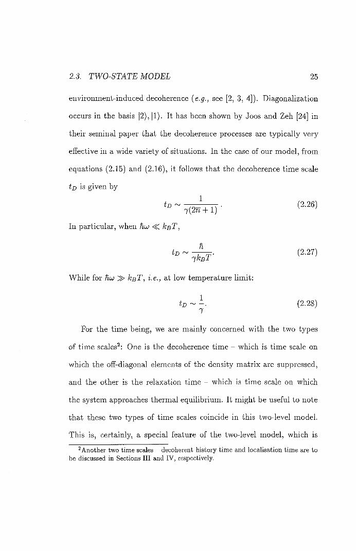
environment-induced decoherence {e.g., see [2, 3, 4]). Diagonalization
occurs in the basis |2), |1). It has been shown by Joos and Zeh [24] in
their seminal paper that the decoherence processes are typically very
effective in a wide variety of situations. In the case of our model, from
equations (2.15) and (2.16), it follows that the decoherence time scale
tjD is given by
~ 7(2n + 1) •
In particular, when hoo <K ksT ,
While for hu> i.e., at low temperature limit:
ZD -J (2.SI8)
7
For the time being, we are mainly concerned with the two types
of time scales^: One is the decoherence time - which is time scale on
which the off-diagonal elements of the density matrix are suppressed,
and the other is the relaxation time - which is time scale on which
the system approaches thermal equilibrium. It might be useful to note
that these two types of time scales coincide in this two-level model.
This is, certainly, a special feature of the two-level model, which is ^Another two time scales - decoherent history time and localisation time are to
be discussed in Sections III and IV, respectively.
26 CHAPTER 2. DECOHERENCE AND PREDICTABILITY
unlikely shared by other models^. It has been found that, for example,
the decoherence time in quantum Brownian motion model is typically
much shorter than the relaxation time [19, 39].
It is easily shown that master equation (2.7) is invariant under uni-
tary transformations of the Lindblad operators:
a I—> UaU\ \—YUa}U\ (2.29)
where is a unitary matrix. Correspondingly, the density operator p
transforms in the same way:
Thus, when t —>• oo
(2.31)
Generally, the density matrix UpsU^ is no longer diagonal. This in-
dicates that environment-induced decoherence does not occur in other
bases. This property is useful on comparison between the environment-
induced decoherence and decoherent histories approaches.
^It is not difEcult to contemplate a two-level model in which those two time scales are different.
2.4. DECOHERENT HISTORIES IN THE TWO-LEVEL SYSTEM MODEL27
2.4 Decoheren t his tor ies in t h e two-level sys t em mode l
2.4.1 Decoherent history analysis
In what follows we shall make a detailed analysis of the decoherent
histories in the two-level model described by the master equation (2.7)
which depicts a Markovian process.
First, let us consider the projection operators represented by
= |1)(1| and = |2>(2| . (2.32)
Obviously, {Pi,i = 1,2} form a set of complete and exclusive projection
operators. Physically, Pi may represent that the atom emits a photon
whereas P2 may represent that the atom absorbs a photon. Then the
decoherence functional at two time points is given by
D[a,d\ = Tr (p„] P^,]) . (2.33)
It is easily shown that, for any 2 x 2 matrix A, the matrix PiAPj (i / j)
is an upper (or a lower) triangle matrix. From equations (2.15),(2.16)
we know that [ • ] propagates the matrix with zero diagonal ele-
ments into the matrix with zero diagonal elements. So, for any initial
density matrix po, the trace in Eq. (2.33) is exactly zero for any dif-
ferent pairs of histories {a ^ a') and for any interval 2 — This
28 CHAPTER 2. DECOHERENCE AND PREDICTABILITY
demonstrates that the set of histories consisting of projectors (2.32)
are exactly decoherent. The generalisation to n time points is straight-
forward. The exact decoherence for any time interval is slightly surpris-
ing. (The density matrix, by contrast, only becomes exactly diagonal
as F -> GO). This exactness is due to the simplicity of the model and
we do not expect it to be a generic feature.
Next, consider more general projection operators which correspond
to the projection to any direction. With any direction denoted by a
unit vector n = (sin ^ cos sin 0 sin ( , cos (/>), we associate a vector |?2)
which belongs to the Hilbert space of the two-level system,
|n) = cos- |1) — e sin - |2) . (2.34)
Then one can define the following projection operators on the Hilbert
space of the system:
/ P+ = |n)(n|, P- = |n ' ) ( " ' l ; (2.35)
where 1? ') is the orthogonal complimentary of \n)-.
\n ') = e ' * 8 i n - | l ) + c o 8 - | 2 ) . (2.36)
We shall show that a set of histories consisting of the projection opera-
tors and P- are approximately decoherent. To this end, first, note
2.4. DECOHERENT HISTORIES IN THE TWO-LEVEL SYSTEM MODEL29
that for any 2 x 2 matrix A,
Tr (P+AP_) = Tr {P-AP+) = 0 . (2.37)
Hence, from (2.17)-(2.20), it can be seen that, after the propagation
of • ], all of the diagonal elements of matrix Kti[P±^'^to[Po]P^]
contain an exponential damping factor
Damping factor = . (2.38)
Thus, we conclude
V a f a ' . (2.39)
This proves that the set of histories consisting of P+,P- are approxi-
mately decoherent if time interval between tk and tk+i is larger than
the characteristic time scale,
decoherence ^ /<-. i 7T' (2.40) 7(2n + 1)
This is an expected result. We will give a more detailed estimate of the
degree of decoherence in the next section.
Note that (decoherence decreases as the coupling 7 is made stronger.
From (2.10), it is easy to see that the decoherence is more effective if
the temperature of bath, T, increases. Conversely, decreasing temper-
ature will make system spend more time to decohere. The maximum
30 CHAPTER 2. DECOHERENCE AND PREDICTABILITY
decoherence time for a set of histories is I / 7 which corresponds to
zero temperature of bath. In this case, the damping is caused by only
spontaneous emission, and then the decoherence process is not very
effective.
In summary, we find exact decoherence of histories characterised by
the projections onto |1) and |2), and approximate decoherence in any
other basis.
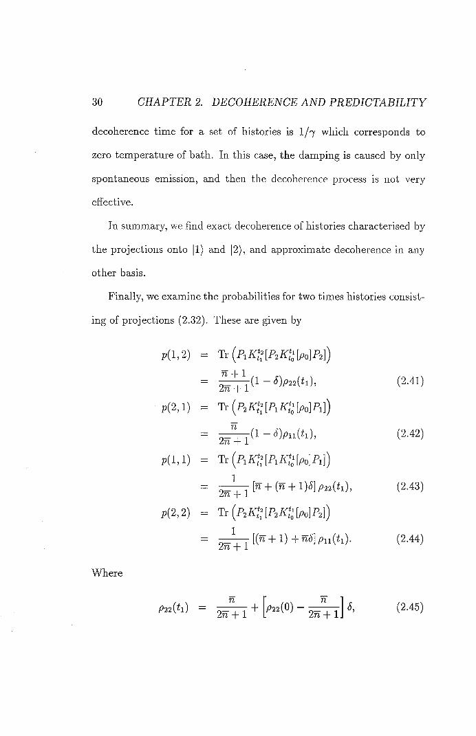
Finally, we examine the probabihties for two times histories consist-
ing of projections (2.32). These are given by
p(i,2) = Ti-{p,k;;ip,k;mp2])
W -U 1 (1 — S)p22(ti), (2.41)
2n -|-1
p(2, l ) = Tr{P2is'f[P,A'J[p„]P,])
n (1 — ^)pii(ti), (2.42)
2n + 1
p ( l , l ) = Tr(P,/^5[FiAX'[p„]Fij)
= 2 [" + (" + 1)< ] ^22(^1), (2.43)
p(2,2) =
= + (2.44)
Where
n
2n + l
n p22{ti) - T + p22{0) - S, (2.45)
2n + IJ
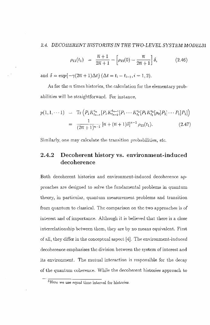
2.4. DECOHERENT HISTORIES IN THE TWO-LEVEL SYSTEM M0DEL31
a, ( 2 j a ) n
^ 2 i T T .
and 5 = exp{—7(2n + l )At} (At = ti — = 1,2).
As for the n times histories, the calculation for the elementary prob-
abilities will be straightforward. For instance,
p( l , 1.. • • 1) = Tr • • • m P i K r , M P i ] • • • P.]P.l)
= (2n + l)»-" + + (2.47)
Similarly, one may calculate the transition probabilities, etc.
2.4.2 Decolierent history vs. environment-induced decoherence
Both decoherent histories and environment-induced decoherence ap-
proaches are designed to solve the fundamental problems in quantum
theory, in particular, quantum measurement problems and transition
from quantum to classical. The comparison on the two approaches is of
interest and of importance. Although it is believed that there is a close
interrelationship between them, they are by no means equivalent. First
of all, they differ in the conceptual aspect [4]. The environment-induced
decoherence emphasises the division between the system of interest and
its environment. The mutual interaction is responsible for the decay
of the quantum coherence. While the decoherent histories approach to
Here we use equal time interval for histories.
32 CHAPTER 2. DECOHERENCE AND PREDICTABILITY
quantum theory permits prediction to be made in genuinely closed sys-
tems, such as the whole universe. Apart from this conceptual difference,
with this two-level system we will be able to see some other interesting
differences. One such difference is that, for any direction |n), the sets
of histories consisting of the projections = |n)(?2| and P_ = \n'){n'\
are decoherent (approximately) for any initial state. However, we have
seen from Section 2.3 that the density matrix tends to become diagonal
only in a particular basis |1), |2). Another intriguing difference is the
time scales in two formulations. As was shown in the previous section,
the histories consisting of the projection onto two levels |1) and |2)
are exactly decoherent for any time, moreover, it is independent of the
initial density matrices. Whereas environment-induced decoherence in
the same basis |1), |2) could only occur after a certain time, which is
dependent on the initial state. From the above we see that those two
formalisms differ enormously in this two-level model.
It should be noted that the differences exhibited here may not be
of generality. It is likely that these differences are purely due to the
simplicity of the model or due to the approximations employed in the
derivation of master equation (such as Born-Markov approximations).
However, at any rate, we have shown, within the domain of applica-
bility of the model presented here, the differences between these two
2.5. DEGREE OF DECOHERENCE AND PREDICTABILITY 33
formalisms are significant. Moreover, our discussions here could serve
as the useful hints for the further studies on more realistic models.
2.5 Degree of decoherence a n d predic tabi l -i ty
In this section we will explicitly estimate the degree of decoherence. We
show that the degree of decoherence is determined by the largest and
the smallest eigenvalues of the projection operators and density matrix
at a certain time (See below Section 2.5.1). By using von Neumann
entropy, we also discuss the predictability and its relation to the upper
bounds of degree of decoherence.
2.5.1 Approximate decoherence
Physically, one would not expect the decoherence takes place exactly.
Therefore the investigation of the approximate decoherence is of im-
portance. In practical problems, one can, at best, only expect that
probability sum rules are satisfied up to order e, for some constant
e < 1. Namely, the interference terms do not have to be exactly zero,
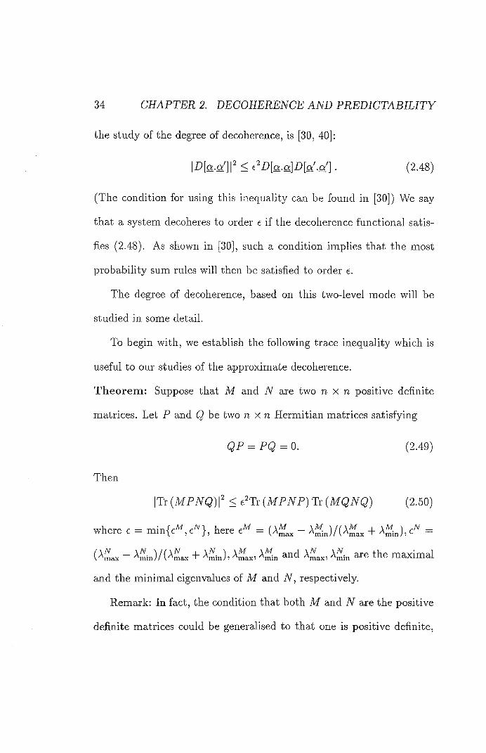
but SOTallerthan probabilities by a factor of e. One simple inequality,
called Dowker-Halliwell criterion, which turns out to be very useful to
34 CHAPTER 2. DECOHERENCE AND PREDICTABILITY
the study of the degree of decoherence, is [30, 40]:
|Z)[a.a']p < [a.a]£)[«'.a'] . (2.48)
(The condition for using this inequality can be found in [30]) We say
that a system decoheres to order e if the decoherence functional satis-
fies (2.48). As shown in [30], such a condition implies that the most
probability sum rules will then be satisfied to order e.
The degree of decoherence, based on this two-level mode will be
studied in some detail.
To begin with, we establish the following trace inequality which is
useful to our studies of the approximate decoherence.
T h e o r e m : Suppose that M and N are two n x n positive definite
matrices. Let P and Q be two n x n Hermitian matrices satisfying
QP = PQ = 0. (2.49)
Then
|Tr ( M f 7VQ) I" < e"Tr ( M f TVf) Tr ( M Q ( 2 . 5 0 )
where e = min{e^, here = ( A ^ - Aj)<^)/(Aj;^ + AjK ), =
A ; aje the maximal
and the minimal eigenvalues of M and N, respectively.
Remark: In fact, the condition that both M and N are the positive
definite matrices could be generalised to that one is positive definite.
2.5. DEGREE OF DECOHERENCE AND PREDICTABILITY 35
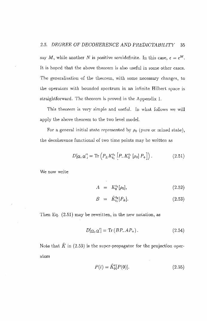
say M, while another N is positive semi definite. In this case, e = e^.
It is hoped that the above theorem is also useful in some other cases.
The generalisation of the theorem, with some necessary changes, to
the operators with bounded spectrum in an infinite Hilbert space is
straightforward. The theorem is proved in the Appendix 1.
This theorem is very simple and useful. In what follows we will
apply the above theorem to the two-level model.
For a general initial state represented by po (pure or mixed state),
the decoherence functional of two time points may be written as
B[s , s ' ] = Tr [p_Ki' [p„] f + j ) . (2.51)
We now write
== (2^52)
(2J)3)
Then Eq. (2.51) may be rewritten, in the new notation, as
a'] = Tr ( g f _ A f + ) . (2.54)
Note that K in (2.53) is the super-propagator for the projection oper-
ators
P(i) = /^5(F(0)]. (2.55)
36 CHAPTER 2. DECOHERENCE AND PREDICTABILITY
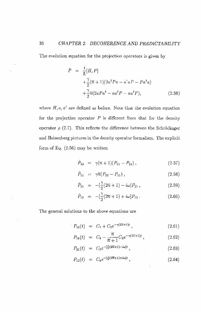
The evolution equation for the projection operators is given by
p =
+ ^(n + l)(2a'^Pa — a^aP — Pa^a)
+ ^n{2aPa^ — aa^P — aa^P), (2.56)
where H, a, a'^ are defined as before. Note that the evolution equation
for the projection operator P is different from that for the density
operator p (2.7). This reflects the difference between the Schrodinger
and Heisenberg pictures in the density operator formalism. The explicit
form of Eq. (2.56) may be written
P22 — 7(M + 1)(-Pii — P22) 5 (2.57)
A i = '7M(f22 - f i i ) , (2.58)
P21 = —[^(2n + 1) — za;]P2i ) (2.59)
P12 = " [ ^ ( 2 » + 1) + iu>]Pi2 • (2.60)
The general solutions to the above equations are
f22(<) = + (2.61)
fn(<) = (2.62) n + i
f2i(() = (2.63)
fi2(<) = (2.64)
2.5. DEGREE OF DECOHERENCE AND PREDICTABILITY 37
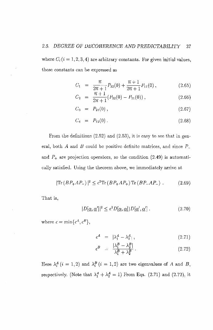
where Q (i = 1,2,3,4) are arbitrary constants. For given initial values,
these constants can be expressed as
rf 4- 1
^2 = ^=-jjy(-P22(0) - Pii(O)) , (2.66)
C3 = ^21(0) , (2.67)
C4 = Pi2(0) . (2.68)
From the definitions (2.52) and (2.53), it is easy to see that in gen-
eral, both A and B could be positive definite matrices, and since P_
and P+ are projection operators, so the condition (2.49) is automati-
cally satisfied. Using the theorem above, we immediately arrive at
|Tr {BP+AP_) I" < e^Tr {BP+AP+) Tr ( 8 f _ A f _ ) . (2.69)
That is,
|-D[a,a']|^ < e '^D[a,a])D[^,^] . (2.70)
where e = min{e^, e-®},
= |A^ —A^l, (2.71)
= i f w -
Here Xf {i = 1,2) and Af {i = 1,2) are two eigenvalues of A and B,
respectively. (Note that Xf + Xf = 1) From Eqs. (2.71) and (2.72), it
38 CHAPTER 2. DECOHERENCE AND PREDICTABILITY
is easily seen that the degree of decoherence may depend on both the
projection operators we use and the initial state of the system. This
is also an expected result. For the two-level system, and can
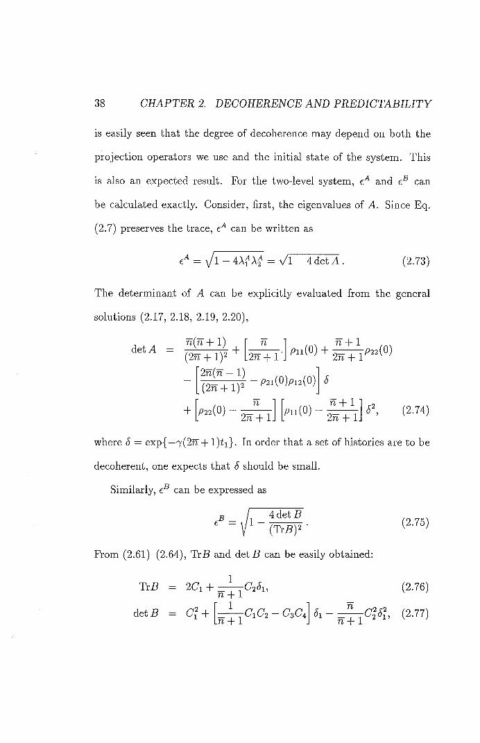
be calculated exactly. Consider, first, the eigenvalues of A. Since Eq.
(2.7) preserves the trace, can be written as
\ / l — 4A^A2 = Vl — 4 det A . (2.73)
The determinant of A can be explicitly evaluated from the general
solutions (2.17, 2.18, 2.19, 2.20),
n(n-h 1) det A
(2n + 1)2
•2n(n + 1)
n
+
(Sin 4- 1):
P22(0)
L2n + 1
P2I(0)PI2(0)
W 4- 1 />ii(0) + ^22(0)
2n + 1'
n
2n + IJ (2.74)
2n + IJ
where S = exp{—7(2n + l)Zi}. In order that a set of histories are to be
decoherent, one expects that 5 should be small.
Similarly, e-® can be expressed as
R 4 det B 11 -
(TTrZ?): '
From (2.61)-(2.64), TiB and det B can be easily obtained:
1
(2.75)
TrB 2Ci +
d e t B = C^ +
n + l 1
n + l C1C2 — C3C4
(2.76)
(2.77)
2.5. DEGREE OF DECOHERENCE AND PREDICTABILITY 39
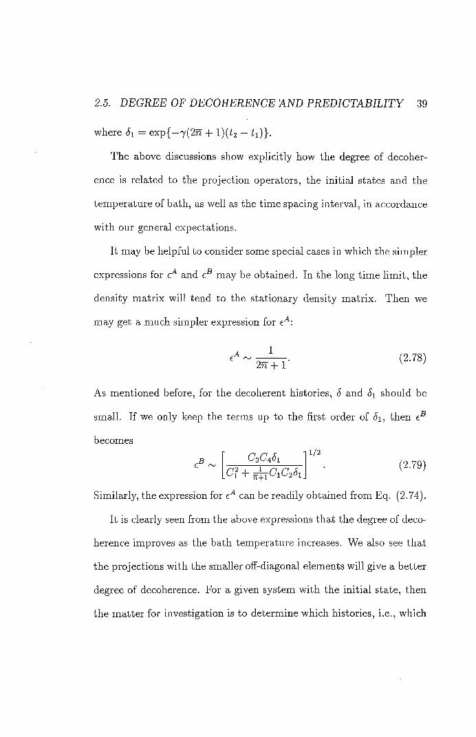
where = exp{—7(2^ + l)(t2 — ^i)}-
The above discussions show explicitly how the degree of decoher-
ence is related to the projection operators, the initial states and the
temperature of bath, as well as the time spacing interval, in accordance
with our general expectations.
It may be helpful to consider some special cases in which the simpler
expressions for and e"® may be obtained. In the long time limit, the
density matrix will tend to the stationary density matrix. Then we
may get a much simpler expression for
- 2 ^ -
As mentioned before, for the decoherent histories, S and should be
small. If we only keep the terms up to the first order of ^i, then e®
becomes 1/2
C2-79)
Similarly, the expression for can be readily obtained from Eq. (2.74).
It is clearly seen from the above expressions that the degree of deco-
herence improves as the bath temperature increases. We also see that
the projections with the smaller off-diagonal elements will give a better
degree of decoherence. For a given system with the initial state, then
the matter for investigation is to determine which histories, i.e., which
40 CHAPTER 2. DECOHERENCE AND PREDICTABILITY
string of projections, will lead to the decoherence condition being sat-
isfied. Therefore, we see that serves as the main criterion for the
degree of decoherence.
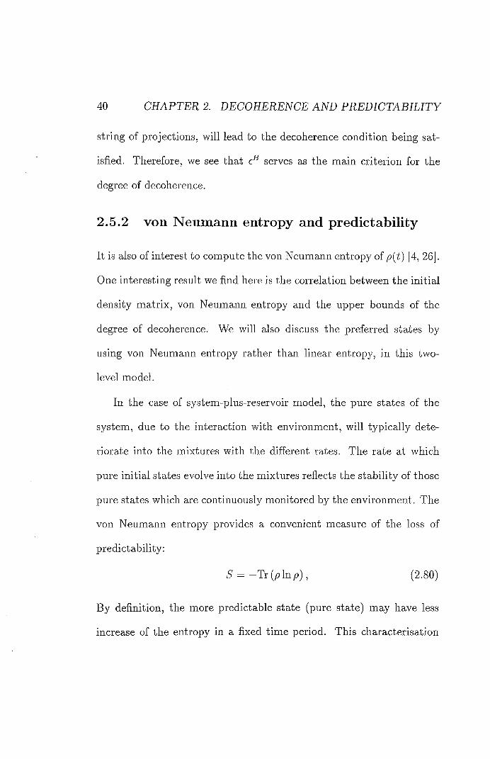
2.5.2 von N e u m a n n entropy and predictability
It is also of interest to compute the von Neumann entropy of p(t) [4, 26].
One interesting result we find here is the correlation between the initial
density matrix, von Neumann entropy and the upper bounds of the
degree of decoherence. We will also discuss the preferred states by
using von Neumann entropy rather than linear entropy, in this two-
level model.
In the case of system-plus-reservoir model, the pure states of the
system, due to the interaction with environment, will typically dete-
riorate into the mixtures with the different rates. The rate at which
pure initial states evolve into the mixtures reflects the stability of those
pure states which are continuously monitored by the environment. The
von Neumann entropy provides a convenient measure of the loss of
predictability:
5 ' = - T r (p lnp) , (2.80)
By definition, the more predictable state (pure state) may have less
increase of the entropy in a fixed time period. This characterisation
2.5. DEGREE OF DECOHERENCE AND PREDICTABILITY 41
process of predictability is called the predictability sieve (coined by
Zurek [4]) which has been studied recently in quantum Brownian mo-
tion model by using the linear entropy [4, 26, 41]. We will see that
two-level system serves as a very nice toy model to employ this "pre-
dictability sieve" by directly using the von Neumann entropy.
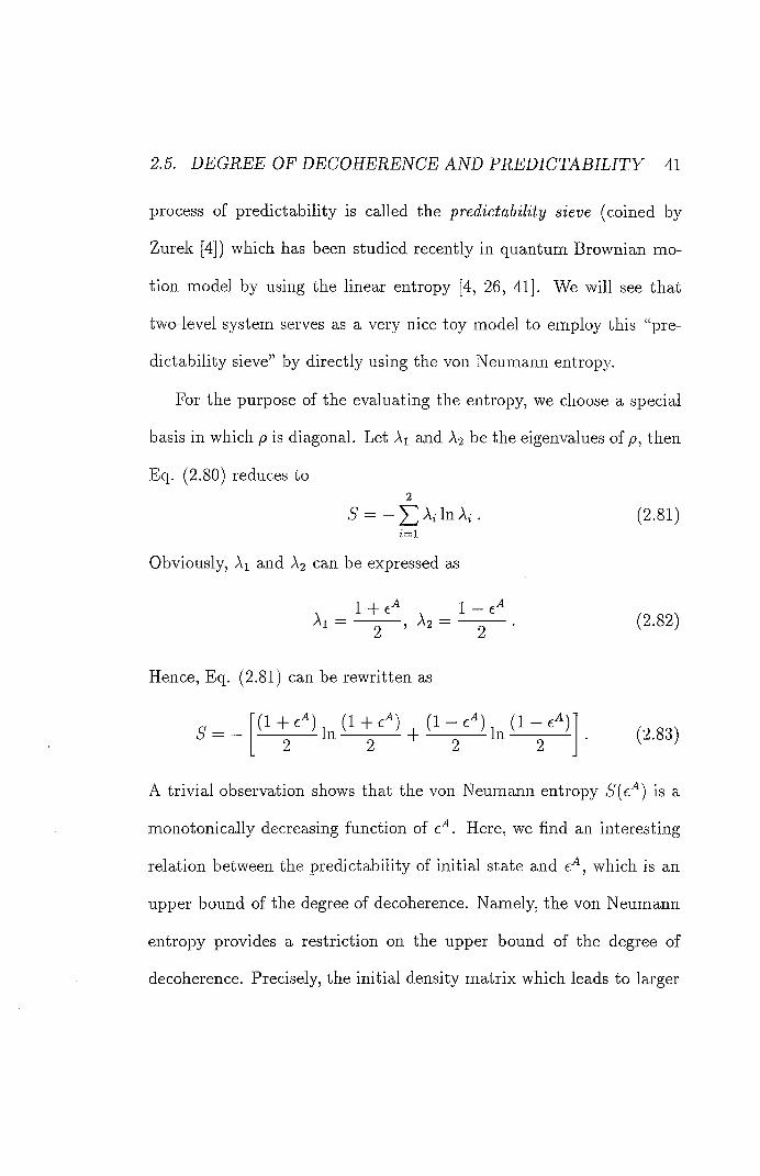
For the purpose of the evaluating the entropy, we choose a special
basis in which p is diagonal. Let Ai and Ag be the eigenvalues of /?, then
Eq. (2.80) reduces to 2
= -- A; . (2Jgl) i=l
Obviously, Ai and A2 can be expressed as
1 1 — Ai = A , = . ( 2 . 8 2 )
Hence, Eq. (2.81) can be rewritten as
S = (1 + (1 + I (1 - (1 - ^^)
( 2 . 8 3 )
A trivial observation shows that the von Neumann entropy S'(e'^) is a
monotonically decreasing function of e^. Here, we find an interesting
relation between the i)redictability of initial state and e^, which is an
upper bound of the degree of decoherence. Namely, the von Neumann
entropy provides a restriction on the upper bound of the degree of
decoherence. Precisely, the initial density matrix which leads to larger
42 CHAPTER 2. DECOHERENCE AND PREDICTABILITY
entropy production may give smaller e^. This relation between the
predictability and the degree of the decoherence is a physically expected
result. To obtain the higher degree of the decoherence one would expect
that the environment has stronger influence on the system of interest,
such as increasing the temperature of the bath. Then the predictability
of the state, correspondingly, decreases.
It is useful to point out here that the actual degree of decoherence
could be much smaller than the upper bound since it is often typi-
cally undercut by the lesser upper bound Moreover, the matter for
investigation in histories approach is to determine which histories will
satisfy the given degree of decoherence. In contrast, our goal here is
merely to see how the initial states are related to the upper bounds of
the degree of decoherence, hence, we do not take any particular set of
histories into account.
Next, by using von Neumann entropy we shall find the most pre-
dictable states, those states will, by definition, generate least entropy
production for a given time interval. Since the entropy S (2.83) is the
monotonically decreasing function of e^, it is equivalent to find the
states which give rise to the largest e^. From (2.73) and (2.74) it is
2.& jDfSCUS&nDN 43
easily seen that
a) = e | l > ± \ f c T T l 2 > (2.84) 2iT + r ' V 2n + 1
minimise the von Neumann entropy, and therefore are the preferred
states. This is slightly surprising from both decoherent histories and
environment-induced decoherence points of view. At first sight, one
might expect that |1) and |2) would be the preferred states, since this
basis plays a very special role in both formalisms. However, from equa-
tions (2.15) and (2.16) it is easy to see that the pure states |1) and |2)
will immediately deteriorate into the mixed states. Namely, those two
states are most vulnerable to the influence of the environment. This
explains why the basis |1) and |2) are not the preferred states.
Also, we see from the above discussions that the states, which di-
agonalize the density matrix, are not necessarily same as the preferred
states that are sorted by the Zurek's predictability sieve.
2.6 Discussion
In this chapter, we have shown that there are a number of sets of
decoherent histories in this two-level model. Clearly, these decoherent
histories are not equally important from physical point of view. Among
those, the most natural one is that which consist of the projections onto
44 CHAPTER 2. DECOHERENCE AND PREDICTABILITY
|1) and 12). We have proven that this set of histories give the best degree
of decoherence. Note that the density matrix in the basis |1) and |2)
will become diagonal after a typically short time.
The approximate decoherence is of basic importance in practical
physical process. By using this two-level system model we can clearly
see what determines the degree of decoherence. For a given set of his-
tories, the only adjustable parameters are the temperature of bath, the
time-spacing interval and the initial state of the system, in accordance
with our general expectations.
We have studied the predictability of the pure states in this two-
level model. The von Neumann entropy in this situation serves as pre-
dictability sieve to sort out the preferred states which yield the smallest
entropy production. As byproduct, we also see an interesting relation
between the upper bound of degree of decoherence and the initial den-
sity operators through the von Neumann entropy.
Finally, there are several special features of our model which are
worth pointing out explicitly. First, the Hamiltonian of the system
is diagonal in the basis |1), |2). We see that the evolution equations
for the diagonal elements and the off-diagonal elements of the density
matrix are decoupled in this situation. One consequence of this is the
exactness of decoherence histories of the projections onto |1), |2). An
2.& jDfSCL/S&RDN 45
immediate generalisation of our model is to consider the Hamiltonian
that does not enjoy this property. One such example is that, in addition
to a thermal radiation field, the two-level atom is applied a coherent
driving field. Notice that, in this situation, the evolution equations
for the diagonal and off-diagonal elements of density matrix are no
longer decoupled. The effect of making this change is that, instead
of decoherence, the quantum coherence could be generated due to the
influence of the coherent driving field [12]. Another special feature is
that the decoherence time and relaxation time scales coincide. This
is perhaps a typical feature of the two level-models. In the quantum
Brownian motion model, the decoherence time is much shorter than
relaxation time [19, 39]. At last, let us note that the coarse-graining
in our two-level system is made by using projection operators on the
system whilst ignoring the environment. It would be interesting to
consider the general 72-dimensional model in which the effect of a further
coarse-graining on the degree of decoherence can be discussed.
Chapter 3
Stochastic Localisation Processes
Alice laughed. "There's no use trying," she said; "One can't believe the impos-sible things." "I dare say you haven't had much prac-tice," said the Queen. "When I was your age, I always did it for half hour a day. Why, sometime I've believed as many as six impossible things before breakfast. . . ."
—Lewis Carroll Through the Looking-Glass
3.1 Unravel l ing of mas t e r equa t ion
It is well known that the master equation provides an ensemble de-
scription of a quantum system. The unravelling of master equation as
the stochastic Schrodinger equation for the state vector, complement-
ing the ensemble description, provide many insights into the foundation
of quantum theory, especially in quantum measurement and the use-
46
3.1. UNRAVELLING OF MASTER EQUATION 47
ful tools to study various practical problems in the quantum optics
{e.g., see [16, 17]). In this chapter we will study the localisation in the
two different unravellings of the master equation - quantum jump sim-
ulation and quantum state diffusion approaches. The former use the
discrete random variables whereas the latter use the continuous random
variables.
3.1.1 Quantum j u m p simulation
In the measurement schemes, such as direct photo-detection, the mas-
ter equation, which models the measurement process, in some sense
describes the lack of information of the systems. Namely, it describes
the measurement process in which the results of measurement are not
extracted. The quantum jump simulations, by contrast, mimic that
Vililck may be observed in a single run of the experiment. The state of
system in this situation is represented by a wave function. The whole
physical process under consideration is the combinations of continuous
evolutions and abrupt jumps which are characterised by the discrete
random variables. Therefore, the wave function of an individual system
is usually governed by a stochastic differential equation. The stochas-
tic unravellings are said to be equivalent to the master equations if the
former after the stochastic average could reproduce the latter. The al-
4:8 3. PftoczosffE:;?
ternative description by a single wave function is not confined in the
measurement processes. In general, any master equation with Lindblad
form [42] can be unravelled into the stochastic Schrodinger equation^.
For the master equation (2.7), the stochastic Schrodinger equation
takes the following form:
+ g " y ) I • (3- )
Here Li = + l)a, L2 = are the Lindblad operators rep-
resenting the influence of the environment and Ni — L^Li {i — 1,2).
{Ni) = {il)\Ni\ijj) represents quantum average and M represents the
ensemble average. The real random variables dWi (% == 1,2) satisfy
dWidWj = 6ijdWi , (3.2)
M{dWi) = {Ni)dt (%==1,2). (3.3)
Under condition (3.2), it is easy to see that dWi only take two values: 0
and 1. The master equation (2.7) can be recovered from the stochastic
Schrodinger equation (3.1) in the sense that if |^) is the solution to Eq.
(3.1) then p = M|V')(^| satisfies master equation (2.7).
^Very recently, Diosi, Gisin and Strunz have described a nonlinear non-Markovian version of quantum state diffusion theory. See [43, 44].
3.i. L /NRAyEIIMG OF MASTER EQL/ATfON 49
In what follows we shall discuss the the 'localisation' properties of
the single jump trajectories. Here, by 'localisation' we mean that the
quantum state vector generated by the stochastic Schrodinger equation
will converge to some fixed states in the mean square .
More precisely, let A be an operator (not necessarily Hermitian),
then we define the quantum mean square deviation as
cr (A,A) = (AtA}-(A'}(A). (3.4)
If the solution of the stochastic Schrodinger equation (3.1) satisfies
M—a{A,A)<0, (3.5)
namely, the dispersion of the operator A tends to decrease as time
evolves. Then we say that the solution localises at the eigenstates of
the operator A [A is sometimes called the collapse operator).
For the stochastic Schrodinger equation for the quantum jump sim-
ulation in two-level system, the collapse operator is cr . Then quantum
mean square deviation in this case is
(Acr^)^ = 1 — {(JzY • (3.6)
In order to prove the localisation, we should first derive the evolution
equation of the expectation value of az by using the following formula:
d{A) = -I- {dij)\A\il)) + , (3.7)
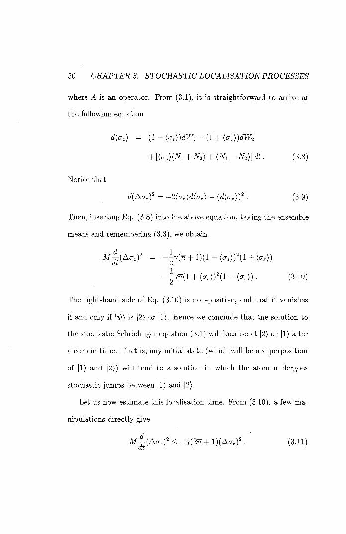
50 CHAPTER 3. STOCHASTIC LOCALISATION PROCESSES
where A is an operator. From (3.1), it is straightforward to arrive at
the following equation
d{o'z) = (1 — {o'z))dWi — (1 + {crz))dW2
+ [(c^)(yVi + N2) + {Ni — VY2)] dt. (3.8)
Notice that
d^Aa^Y — ~'^{'^z)d{crz) — (< ((7 )) • (3.9)
Then, inserting Eq. (3.8) into the above equation, taking the ensemble
means and remembering (3.3), we obtain
= —^7(^+ 1)(1 - (crz))^(l + (cTz))
27^(1 + ((^z))^(l ~ i^z)) • (3.10)
The right-hand side of Eq. (3.10) is non-positive, and that it vanishes
if and only if \ij ) is |2) or |1). Hence we conclude that the solution to
the stochastic Schrodinger equation (3.1) will localise at |2) or |1) after
a certain time. That is, any initial state (which will be a superposition
of |1) and |2)) will tend to a solution in which the atom undergoes
stochastic jumps between |1) and |2).
Let us now estimate this localisation time. From (3.10), a few ma-
nipulations directly give
M^(Acr^)^ < -7(2n-1- l)(Acr^)^ . (3.11)
3.1. UNRAVELLING OF MASTER EQUATION 51
So the localisation rate localization is
^localization ~ /Q . \ 5 ( 3 . 1 2 )
7(2n + l)
which agrees with the decoherence time scale (2.26). Note that this is
the minimum localisation time. The actual time for localisation might
be larger than this time.
In some sense, that the localisation in quantum jump simulation
chooses the basis |1), |2) appears to be natural, since they correspond
to the trajectories that would actually observed in an individual experi-
ment. As expected, the set of histories consisting of projection onto the
basis give the best degree of decoherence. In addition, we have seen that
density matrix become diagonal in this basis. Here, we have demon-
strated a close connection between the different approaches. This is
the main results in the paper. The connection we have established here
bridges the two different approaches-decoherent histories and quantum
jump simulations. The former is regarded as a fundamental theory
with a wide range of api^licability, whilst the latter is mainly seen as a
tool with the great practical values, in particular, in the computational
aspects.
Finally, let us compute the evolution of the populations of the two
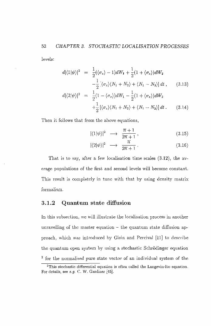
52 CHAPTER 3. STOCHASTIC LOCALISATION PROCESSES
levels:
~2 + %) + (^1 — %)] dt, (3.13)
+ - + (^1 — %)] • (3.14)
Then it follows that from the above equations,
I C W I ' - S t ' (3.15)
^ (3.16)
That is to say, after a few localisation time scales (3.12), the av-
erage populations of the first and second levels will become constant.
This result is completely in tune with that by using density matrix
formalism.
3.1.2 Quantum state diffusion
In this subsection, we will illustrate the localisation process in another
unravelling of the master equation - the quantum state diffusion ap-
proach, which was introduced by Gisin and Percival [11] to describe
the quantum open system by using a stochastic Schrodinger equation
^ for the normalised pure state vector of an individual system of the
^This stochastic differential equation is often called the Langevin-Ito equation. For details, see e.g. C. W. Gardiner [45].
3J. [/NRAVEILfNG OF MASTER EQLIATfON 53
ensemble. Similar to the quantum jump simulation, a solution of the
Langevin-Ito equation for the diffusion of a pure quantum state in state
space represents a single member of an ensemble whose density operator
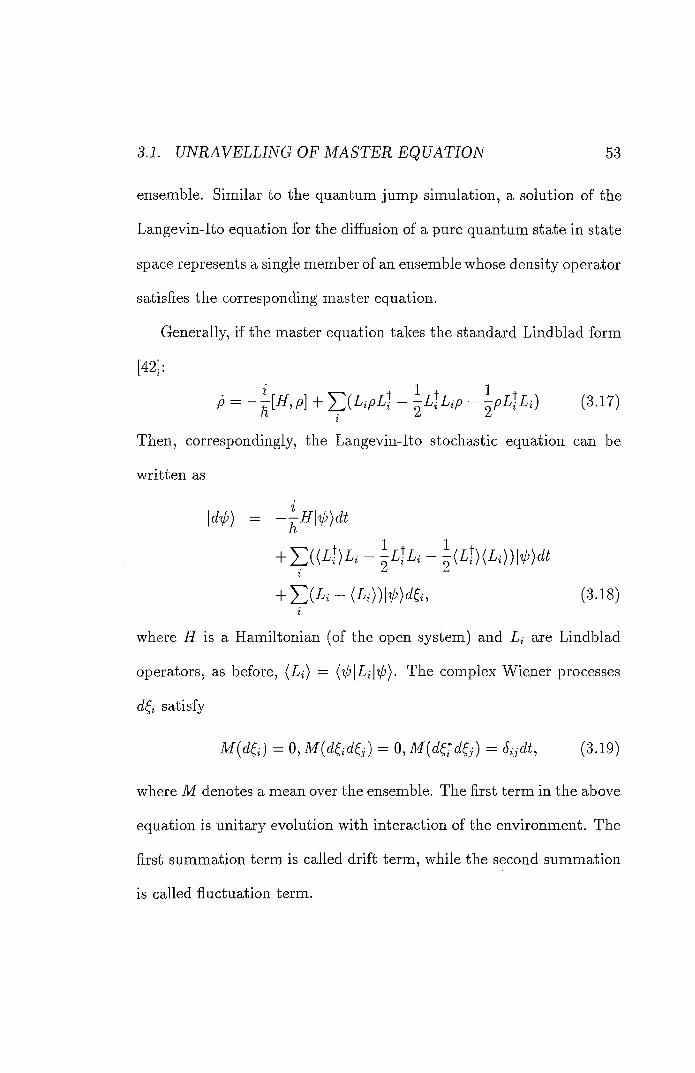
satisfies the corresponding master equation.
Generally, if the master equation takes the standard Lindblad form
P — + '^{LipLl — -L^Lip — -pL\Li) (3.17)
Then, correspondingly, the Langevin-Ito stochastic equation can be
written as
\d'^) = ——H\ip)dt
+ E ( ( 4 > i . - - \{i^)(L,))mt
+ (3.18)
where is a Hamiltonian (of the open system) and Li are Lindblad
operators, as before, {Li) = ('0|Li|'0). The complex Wiener processes
d^i satisfy
M[d(i) = 0 , M(d^id^j) = 0 , M{d^*d^j) = 5ijdt, ( 3 . 1 9 )
where M denotes a mean over the ensemble. The first term in the above
equation is unitary evolution with interaction of the environment. The
first summation term is called drift term, while the second summation
is called fluctuation term.
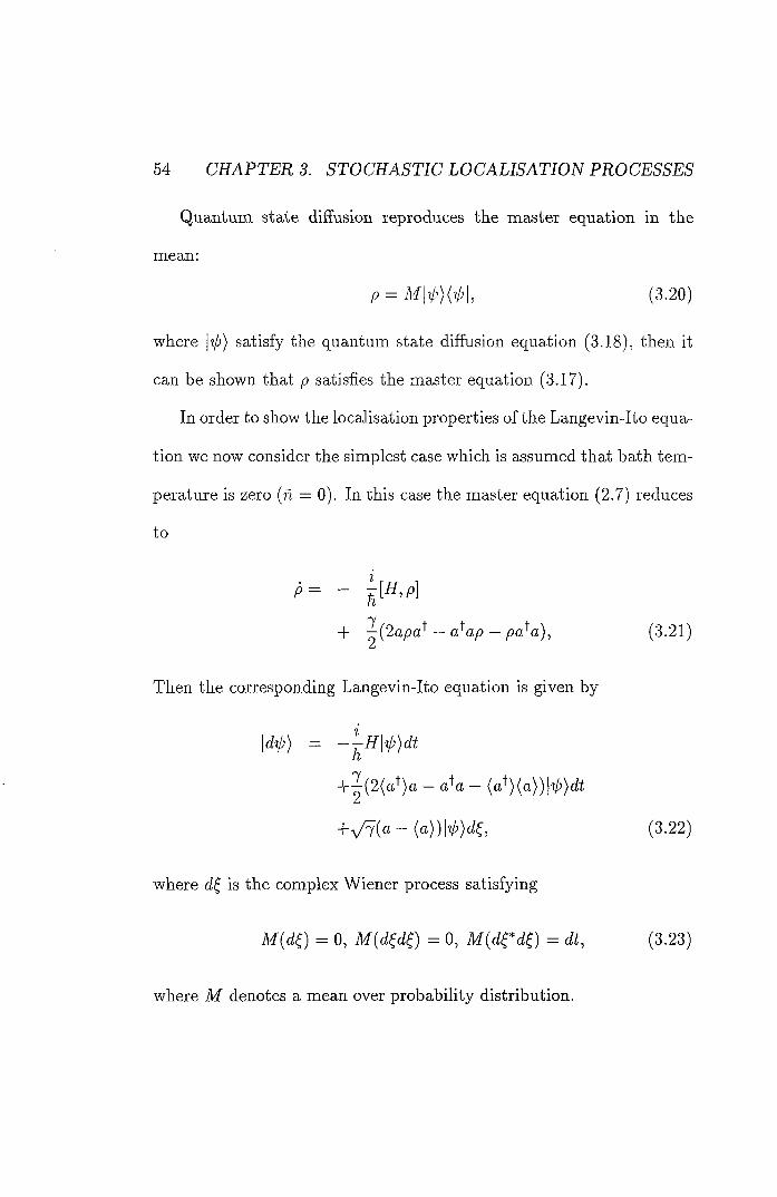
54 CHAPTER 3. STOCHASTIC LOCALISATION PROCESSES
Quantum state diffusion reproduces the master equation in the
mean:
p = M|^)(V'|, (3.20)
where \ip) satisfy the quantum state diffusion equation (3.18), then it
can be shown that p satisfies the master equation (3.17).
In order to show the localisation properties of the Langevin-Ito equa-
tion we now consider the simplest case which is assumed that bath tem-
perature is zero (n = 0). In this case the master equation (2.7) reduces
to
p = - j i f f . Pi
+ ^{2apa^ — a^ap — pa^a), (3.21)
Then the corresponding Langevin-Ito equation is given by
\d^|J) — ——H\tp)dt
— a^a — {a^){a))\'il))dt
+V9(a - (3.22)
where is the complex Wiener process satisfying
M(( ) = 0, M(d^(f^) = 0, M(drc(^) = (ft, (3.23)
where M denotes a mean over probability distribution.
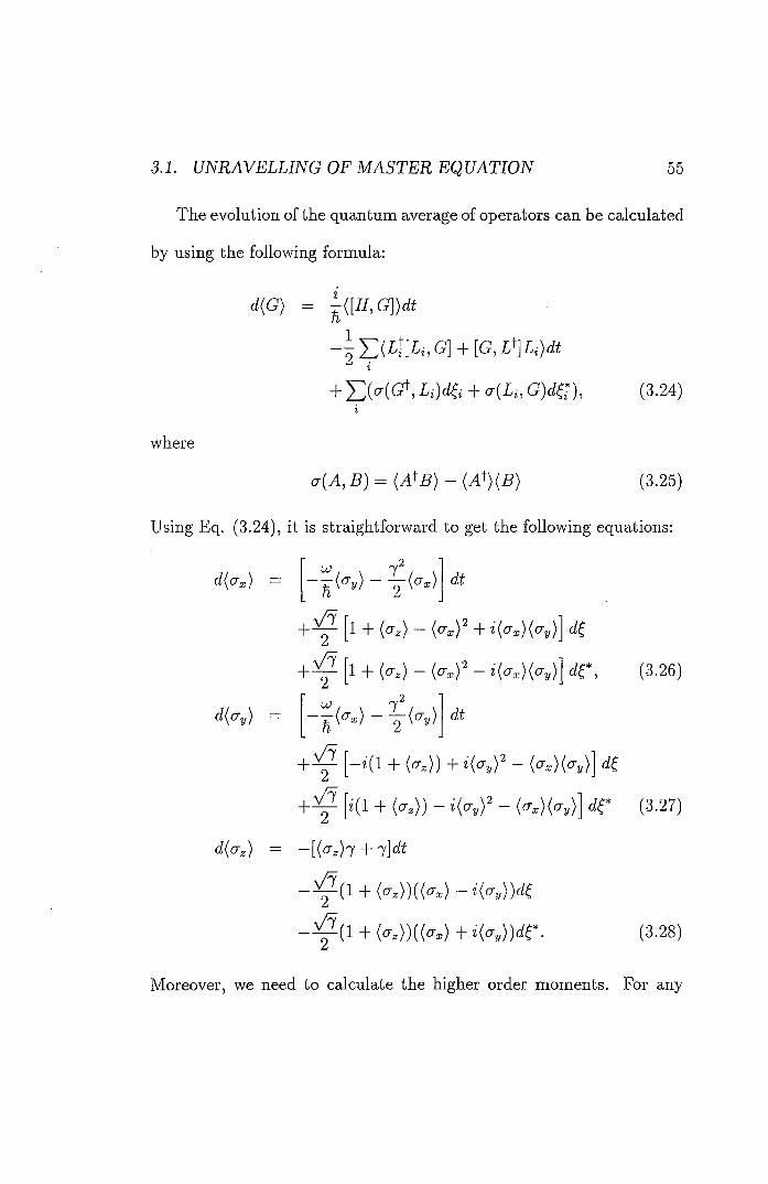
3.1. UNRAVELLING OF MASTER EQ UATION 55
The evolution of the quantum average of operators can be calculated
by using the following formula:
— - ^(Lj[Li, G] + [G, L^Li)dt i
+ j;,(a(G\Li)d(i+<T(L„G)d(n, (3,24)
where
(J {A, B) = {A^B} - {A^){B) (3.25)
Using Eq. (3.24), it is straightforward to get the following equations:
d{ CTr. dt
Vl 2
(3.26)
2
1 + (<7z) — {( xY + i{(^x){(^y) di
1 + (Cz) — {'^xY — i{<^x){<^y)
dt
—i{l + {az))+i{o-yy — {<rx){ay) d(
%(1 + (o-;:)) - (3-27)
d{a^) = -[{a^)-f +'y]dt
Vl 2
(1 + (crz))((o'z> -i((Z^))(^(
(1 + (a;:))(((7^) + z(o-y))(fr- (3.28)
Moreover, we need to calculate the higher order moments. For any
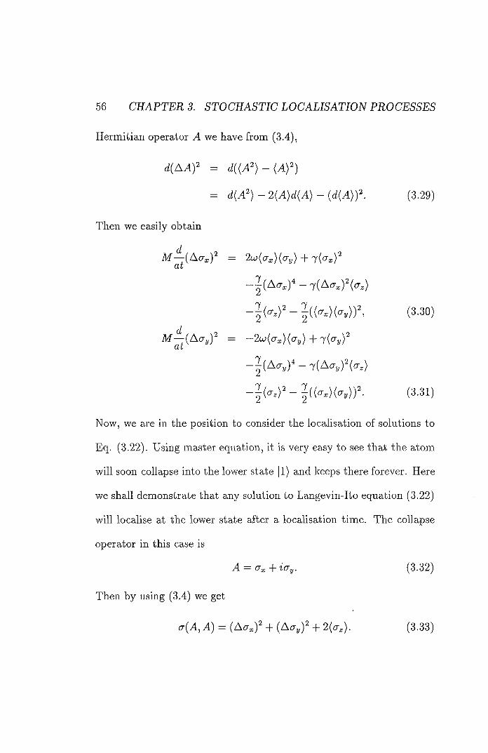
56 CHAPTER 3. STOCHASTIC LOCALISATION PROCESSES
Hermitian operator A we have from (3.4),
= - 2(A)(f(A) - (3.29)
Then we easily obtain
M^(Ao-^)^ = 2w((7^)((Zy) + 'y((7^)^
, (3.30)
M^(A(7^)^ = -2w((7^)((7y)+'Y((7y)^
- ^((':^r)(o'y))^. (3.31)
Now, we are in the position to consider the localisation of solutions to
Eq. (3.22). Using master equation, it is very easy to see that the atom
will soon collapse into the lower state |1) and keeps there forever. Here
we shall demonstrate that any solution to Langevin-Ito equation (3.22)
will localise at the lower state after a localisation time. The collapse
operator in this case is
A = (Ta; + iay. (3.32)
Then by using (3.4) we get
(7(A, A) = (A(Ta;) + (Actj,)^ + 2((j^). (3.33)
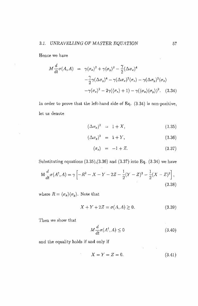
3.1. UNRAVELLING OF MASTER EQUATION 57
Hence we have
+ lf{cryy -dt
2
-l{<^zY ~ ^^((O'z) + 1) — l{{(^x){(^y)Y• (3.34)
In order to prove that the left-hand side of Eq. (3.34) is non-positive,
let us denote
(Acr^)^ = l + X, (3.35)
(AaJ^ = 1 + y , (3.36)
{'^z) — —'1 4- Z. (3.37)
Substituting equations (3.35),(3.36) and (3.37) into Eq. (3.34) we have
d
dt
„.o 1 A) = -Y - X - y - 2Z - - ( y - Z)^ - - ( X - ^)
2 ' ' 2
(3.38)
where R = {crx){(Jy). Note that
X + y + 2Z = (7(A, A) > 0. (3.39)
Then we show that
M ^ ( 7 ( A \ A ) < 0 (3.40)
and the equality holds if and only if
% = y = z = 0. (3.41)
f)8 3. 2^()(:vijLf(L4LT'jrc)ff Pftocj5s:.sj3(?
That is, the average in the left hand sides of equations (3.35), (3.36),
and (3.37) is taken over the ground state |1). This proves that the so-
lution to Eq. (3.22) will localise at the ground state when the evolution
time is larger than the localisation time.
Finally, let us estimate the localisation rate of the quantum state
evolution. Using Eq. (3.38) and Eq. (3.39), we immediately obtain
M^(7(A, A) < -7 (a (A , A))":. (3.42)
So the localisation rate localization is
^local ization ^ • ( 3 . 4 3 )
7
In summary, we have shown the localisation process in both quan-
tum jump simulation and quantum state diffusion. Those localisations
have been extensively discussed in the quantum state diffusion ap-
proaches. Here we have seen that the similar localisation process could
also occur in the quantum jump simulation. It should be noted that,
in the case of the zero-temperature of our two-level model, for any ini-
tial state of the system, the atom will eventually localise at the ground
state. Therefore, the system will always evolve from a pure state into
the pure state. In this sense we say that the decoherence and localisa-
tion are basically trivial in this case. However, the above demonstration
of localisation can still be regarded as a useful example for showing that
3.1. UNRAVELLING OF MASTER EQUATION 59
quantum state diffusion picture provides a consistent description with
the density matrix formalism and decoherence approach.
It is interesting to compare the master equation formulation with
their stochastic unravellings. Clearly, the master equations provide a
fundamental description of the quantum open systems. But numer-
ical simulation of the many-freedom problems seems rather awkward
due to occupying the large memory of computer. Moreover, it cannot
provide a description for an individual system. The quantum trajec-
tories approaches-the unravelling of master equation as the stochastic
Schrodinger equation could do this job and have advantages over mas-
ter equation in computational aspect [11, 46]. For this two-level model,
the merit of stochastic unravellings is mainly in conceptual aspects.
Generally, the localisation process is very difficult to show analytically,
if not impossible.
Obviously, the unravelling of master equation is not unique. Quan-
tum jump simulations and quantum state diffusions are only two well-
known examples, which lie in our interests in this paper. These stochas-
tic unravellings are often connected with the certain measurement schemes.
For instance, the quantum jump simulation can be associated with the
direct photo-detection, and quantum state diffusion corresponds to the
heterodyne detection. In a quantum jump process, quantum jump sim-
ulation may be a natural candidate for description of the process. The
quantum state diffusion by nature is continuous diffusion precess. How-
ever, if the transition is so fast that the "diffusion" from one level to
the other level of atom can be regarded as an instantaneous process,
then quantum state diffusion could also give rise to the "jump" process
[13, 16]. It should be noted that the applicability of quantum jump
simulation and quantum state diffusion are different. The preference of
these stochastic approaches are largely dependent on the physical mod-
els employed and the problems to be solved. In general, the relation
between those two approaches is by no means obvious. Undoubtedly,
the researching into this relation would be of importance and of interest
[47].
3.2 Discussion
In this chapter, based on the two-level system models presented in the
last chapter, we have studied quantum jump simulation and quantum
state diffusion. We have demonstrated the localisation in both quantum
jump simulations and quantum state diffusion approaches. Here we
conclude with a summary and a few remarks.
On combining the results in the last chapter, in which we have
shown that the most natural set of histories is that which consist of
&2. DISCUSSION 61
the projections onto |1) and |2). We have proven that this set of histo-
ries give the best degree of decoherence. Note that the density matrix
in the basis |1) and |2) will become diagonal after a typically short
time. Remarkably, we have shown, in this chapter, that the solutions
to the stochastic Schrodinger equation in the quantum jump simulation
will localise at |1) or |2) after certain time which is basically same as
the decoherence time. Also, we have shown the localisation process in
quantum state diffusion in the case of zero temperature. Our results
have demonstrated a close connection between the decoherent histo-
ries and quantum jump simulation approaches, knowing that the two
approaches have totally different origins^.
In addition, we have found that the environment-induced decoher-
ence, decoherent histories and the localisation process are more effective
as the bath temperature increases. Physically, this is an expected re-
sult as the bath at a higher temperature would have stronger influence
on the system. These results are in agreement with former studies on
the quantum Brownian models [19] as well as on the quantum optical
models [35].
It is important to notice that, as phenomenological theories, both
quantum state diffusion and quantum jump simulation must be used
®This connection has been independently proved by T. Brun [48]. For a recent review, see M. Plenio and P. Knight [49].
under some conditions {e.g., see [13]). The comparison between dif-
ferent approaches therefore must be made in caution since the corre-
spondence between them is by no means mathematically one-to-one
correspondence. Rather, we emphasise that, underlying the quantum
open system, the mutual influence between the system and its envi-
ronment is the common theoretical base of all of those approaches and
both decoherence and localisation are nothing more than the different
manifestations of a single entity.
The environment-induced decoherence, decoherent histories as well
as various stochastic Schrodinger equations have provided many im-
portant insights into the understanding of fundamental problems in
quantum theory. The investigation into the similarity and difference
between the different approaches is of importance. The more thorough
studies in this aspect would be useful.
Chapter 4
Quantum Brownian motion
"... there is a pleasure in recog-nising the old things from a new point of view."
—Richard Feynman An Abstract from "Space-Time Approach to Non-Relativistic Quantum Mechanics"
In the previous two chapters, the quantum two-level system, being
taken as a typical quantum open system, has been studied in some
details. As we emphasised before, analysis of the decoherence is rather
mathematical involved, and it is often very difficult, if not impossible, to
find an exact solutions of the problems. For a deepening understanding,
however, the exact soluble models are always useful. Besides two-level
systems, quantum Brownian motion(QBM) model is another widely
used model in quantum decoherence, quantum dissipation, statistical
physics in general etc [50, 51, 52, 53]. In the following sections we will
provide an alternative derivation of the master equation of QBM.
63
64 CHAPTER 4. Q[7ANT[/MBR0WNfAN MOTION
4.1 I n t r o d u c t i o n
Quantum Brownian motion (QBM) models provide a paradigm of open
quantum systems that has been very useful in quantum measurement
theory [54], quantum optics [12] and decoherence [9, 30, 55]. One of the
advantages of the QBM models is that they are reasonably simple, yet
sufficiently complex to manifest many important features of realistic
physical processes.
Central to the study of QBM is the master equation for the reduced
density operator of the Brownian particle, derived by tracing out the
environment in the evolution equation for the combined system plus
environment. A variety of such derivation have been given [56, 57, 58,
59]. The most general is that of Hu, Paz and Zhang [60, 61], who
used path integral techniques and in particular, the Feynman-Vernon
influence functional.
The purpose of this chapter is to provide an alternative and ele-
mentary derivation of the Hu-Paz-Zhang master equation for QBM, by
tracing the evolution equation for the Wigner function of the whole
system.
This chapter is planned as follows. In Section 4.2, the quantum
Brownian motion model is presented and a derivation of Fokker-Planck
4.2 MASTEREQL/ATfONFOR QI7ANT[/MBROWNfANMOTfON65
equation governing the evolution of Wigner functions of the system of
interest is given. In Sections 4.3 and 4.4, the determination of coeffi-
cients of the master equation for the general case and particular case
are given\ respectively.
4.2 M a s t e r equa t ion for q u a n t u m Brown-ian mo t ion
The system we considered is a harmonic oscillator with mass M and
bare frequency (1, in interaction with a thermal bath consisting of a set
of harmonic oscillators with mass and natural frequency The
Hamiltonian of the system plus environment is given by
2M + -MVi^q^ + ^ C'ngn , (4.1)
where and are the coordinates and momenta of the Brownian
particle and oscillators, respectively, and Cn are coupling constants.
The state of the combined system (4.1) is most completely described
by a density matrix p{q^ qi] q', q[^t) where g, denotes (gi, ...g/f), and p
evolves according to
p = -^[H,p\. (4.2)
^Another method of determining the coefficients of the master equation by using the Laplace transform will be given in Appendix 2.
66 (jd/LPfTCfAf AfOGTfOjV
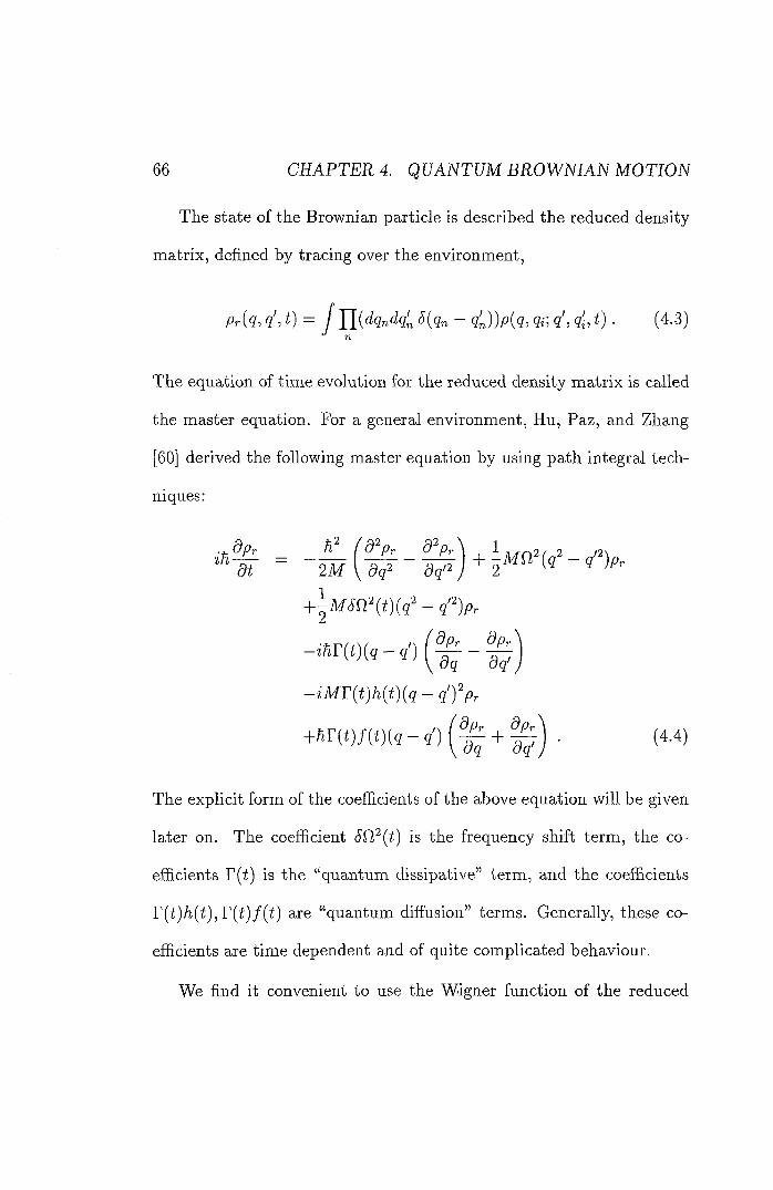
The state of the Brownian particle is described the reduced density
matrix, defined by tracing over the environment,
= y ' (4-3)
The equation of time evolution for the reduced density matrix is called
the master equation. For a general environment, Hu, Paz, and Zhang
[60] derived the following master equation by using path integral tech-
niques:
— q'^)pr
-zMT{t)h{t)(q- q'Ypr
+ar(t)y(t)(g - ?') . (4.4)
The explicit form of the coefficients of the above equation will be given
later on. The coefficient SD,' {t) is the frequency shift term, the co-
efficients r{t) is the "quantum dissipative" term, and the coefficients
r(t)/i(i5), r ( t ) / ( t ) are "quantum diffusion" terms. Generally, these co-
efficients are time dependent and of quite complicated behaviour.
We find it convenient to use the Wigner function of the reduced
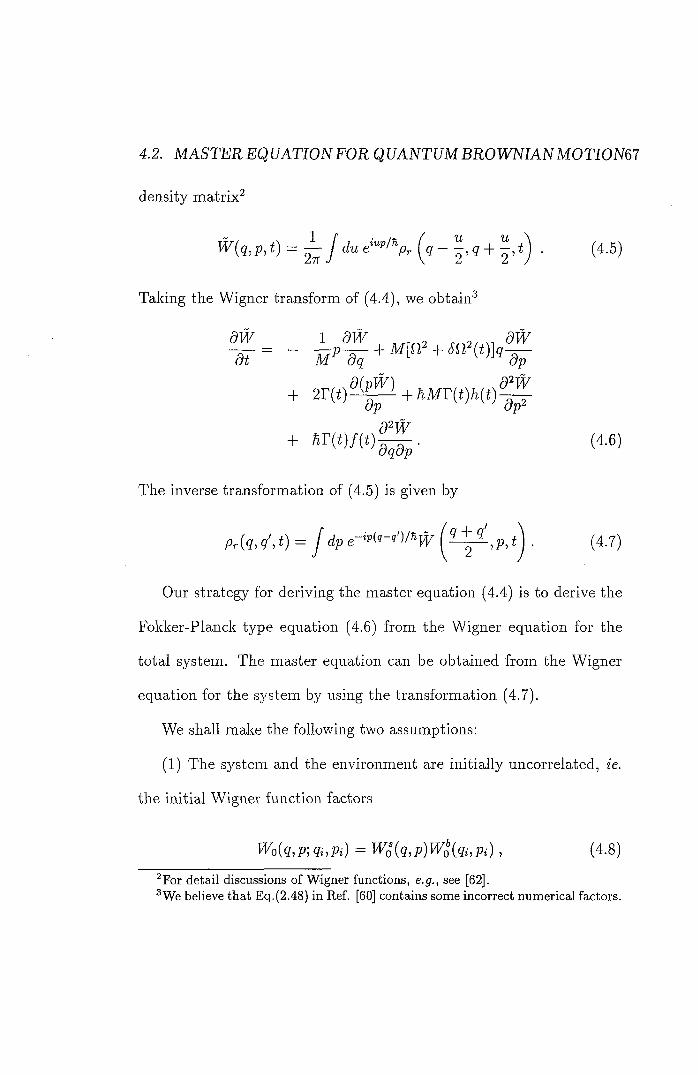
4.2. MASTER EQ UATION FOR Q UANTUM BROWNIAN MOTION67
density matrix^
W(<l,p,t) = ^ f due<"'\ . (4.5)
Taking the Wigner transform of (4.4), we obtain^
f = - i - t
+ 2 r ( t ) ^ + R M r ( t ) f c w | ^
+ (4.6)
The inverse transformation of (4.5) is given by
e-v(9-9')/R][y
Our strategy for deriving the master equation (4.4) is to derive the
Fokker-Planck type equation (4.6) from the Wigner equation for the
total system. The master equation can be obtained from the Wigner
equation for the system by using the transformation (4.7).
We shall make the following two assumptions:
(1) The system and the environment are initially uncorrelated, ie.
the initial Wigner function factors
, (4.8)
^For detail discussions of Wigner functions, e.g., see [62]. ®We believe that Eq.(2.48) in Ref. [60] contains some incorrect numerical factors.
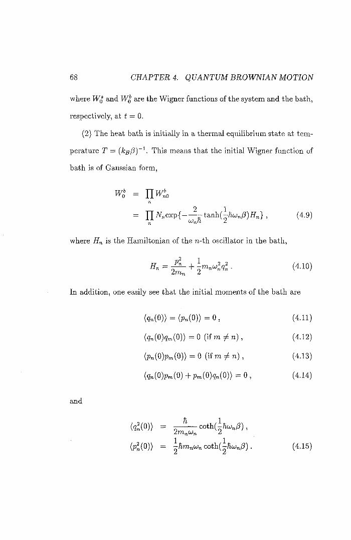
68 CHAPTER 4. QUANTUM BROWNIAN MOTION
where Wq and are the Wigner functions of the system and the bath,
respectively, at t = 0.
(2) The heat bath is initially in a thermal equilibrium state at tem-
perature T = This means that the initial Wigner function of
bath is of Gaussian form,
Wo' = n»'« 6 nO
n
2 1 = n A^»exp{ - ta ,nh. { -hu}nP)Hn} , (4.9)
where Hn is the Hamiltonian of the n-th oscillator in the bath,
% = + . (4.10) 2m„ 2
In addition, one easily see that the initial moments of the bath are
(g . (o)> = (Pn(o)) = o , (4.11)
(%(0)gm(0)) = 0 (if m 7 n) , (4.12)
(Pn(O)pm(O)) ==0 (if m n) , (4.13)
(gn(O)pm(O) + Pm(0)g„(0)) = 0 , (4.14)
and
(Pn(0)) = ^huinU^n COth{^hUn(3) . (4.15)
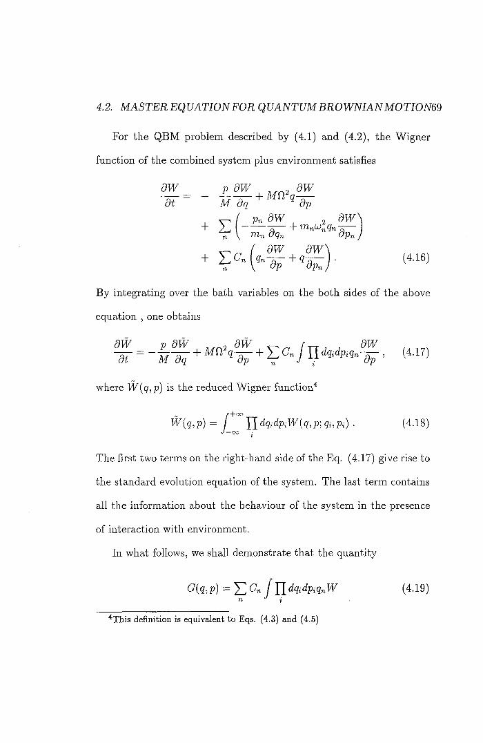
4.2. MASTER EQ UATION FOR Q UANTUM BROWNIAN M0TI0N&9
For the QBM problem described by (4.1) and (4.2), the Wigner
function of the combined system plus environment satisfies
6% ' a? ^
By integrating over the bath variables on the both sides of the above
equation , one obtains
where W{q,p) is the reduced Wigner function^
f+ 00 _ ^ ( g , p ) = / (4-18)
The first two terms on the right-hand side of the Eq. (4.17) give rise to
the standard evolution equation of the system. The last term contains
all the information about the behaviour of the system in the presence
of interaction with environment.
In what follows, we shall demonstrate that the quantity
(?(g,p) = J YidqidpiqnW (4.19)
^This definition is equivalent to Eqs. (4.3) and (4.5)
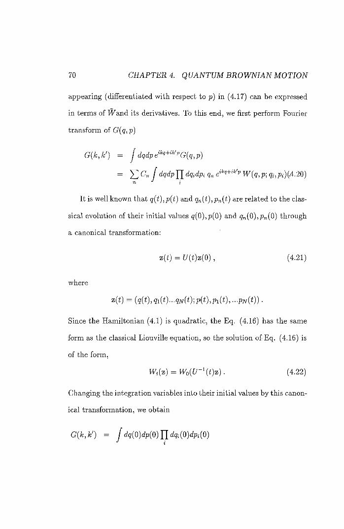
70 CHAPTER 4. Q UANTUM BROWNIAN MOTION
appearing (differentiated with respect to p) in (4.17) can be expressed
in terms of IVand its derivatives. To this end, we first perform Fourier
transform of G{q,p)
= J n W{q, p\ g„p,)(.4.20)
It is well known that q{t),p{t) and qn{t), Pnii) are related to the clas-
sical evolution of their initial values g(0),p(0) and g„(0), j9„(0) through
a canonical transformation;
z(t) = [/(t)z(O) , (4.21)
where
z(<) (g((),gi(^)...gN(^);p((),Pi(^),...PN(()).
Since the Hamiltonian (4.1) is quadratic, the Eq. (4.16) has the same
form as the classical Liouville equation, so the solution of Eq. (4.16) is
of the form,
W,(z) = M/o([/-X()z). (4.22)
Changing the integration variables into their initial values by this canon-
ical transformation, we obtain
G{k,k') = J dq{0)dp{0)Y[dqi{0)dpi{0)
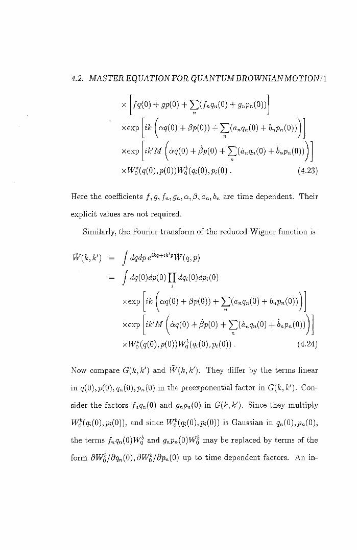
4.2. MASTER EQUATION FOR QUANTUM BROWNfANMOTfOjWl
X /g(0) + gp(0) + ^ (Agn(O) + 9nPn(0))
xexp
xexp
1^0:9(0) + ^p(O)) + ^(Ongn(O) + 6nPn(0))
ik'M (aq{0) + /3p(0) + X^(a„gn(0) + Kpn{0))
x;yj(g(o),p(o))w;^(%(o),p,(o). (4.23)
Here the coefficients f^g,fnign,o:,P,an,bn are time dependent. Their
explicit values are not required.
Similarly, the Fourier transform of the reduced Wigner function is
= I c;g(0)c(p(0) %% (ig,(0)(fp, (0) i
ik (a:g(0) + ,9p(0)) + ^(angn(O) + 6nPn(0)) xexp
xexp ik'M ( 6g(0) + Pp(0) + ^(6^9^(0) + Lpn(O))
xw;^(g(0),X0))w;^(%(0),pX0)). (4.24)
Now compare G(k,k') and W{k,k'). They differ by the terms linear
in < ? ( 0 ) , p ( 0 ) , 5 r i ( 0 ) , P n ( 0 ) in the preexponential factor in G{k,k'). Con-
sider the factors /n?n(0) and gnPn{0) in G{k^k'). Since they multiply
W^o(gi(0),]?i(0)), and since M/^(%(0),p,(0)) is Gaussian in gn(0),p„(0),
the terms /ngn(0)M^ and fi'nPn(0)M^o may be replaced by terms of the
form 5W^o/5g„(0),(9WoV^Pn(0) up to time dependent factors. An in-
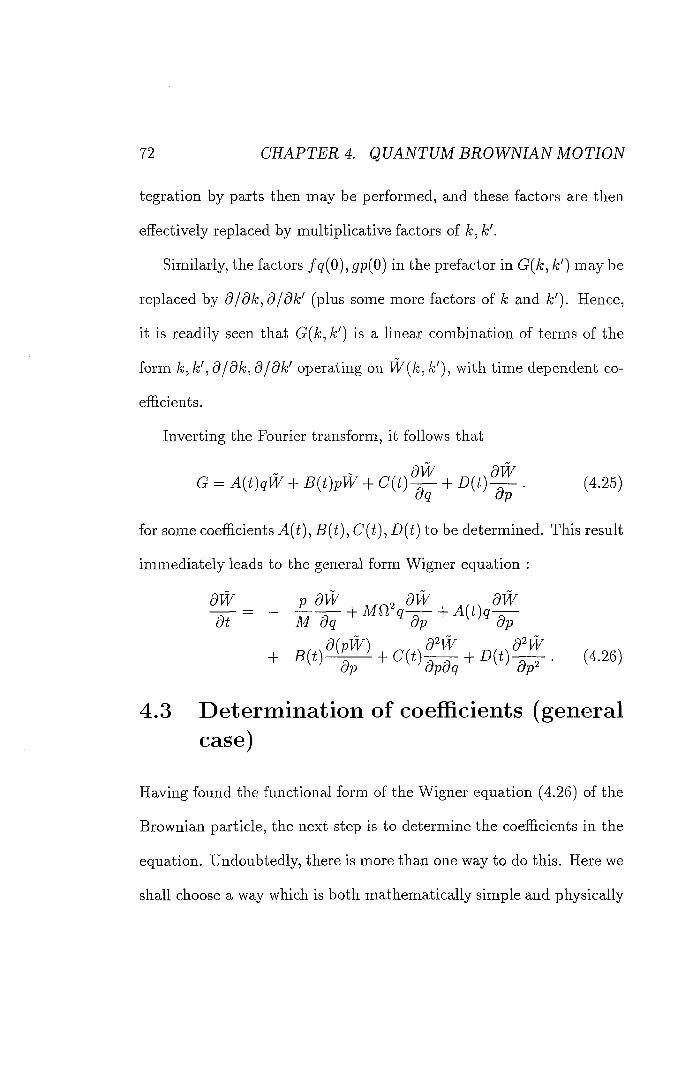
72 CHAPTER 4. Q UANTUM BROWNIAN MOTION
tegration by parts then may be performed, and these factors are then
effectively replaced by multiplicative factors of k, k'.
Similarly, the factors fq(0)^gp(0) in the prefactor in G(k^ k') may be
replaced by d/dk,d/dk' (plus some more factors of k and k'). Hence,
it is readily seen that G{k^ k') is a linear combination of terms of the
form k, k', d/dk,d/dk' operating on W{k, fe'), with time dependent co-
efficients.
Inverting the Fourier transform, it follows that
G = - (4-25)
for some coefficients A(i), B{t), C{t), D{t) to be determined. This result
immediately leads to the general form Wigner equation :
§ - - i f - " . ! - « » . f
* « . . T " " S i - " • » >
4.3 D e t e r m i n a t i o n of coefficients (general case)
Having found the functional form of the Wigner equation (4.26) of the
Brownian particle, the next step is to determine the coefficients in the
equation. Undoubtedly, there is more than one way to do this. Here we
shall choose a way which is both mathematically simple and physically
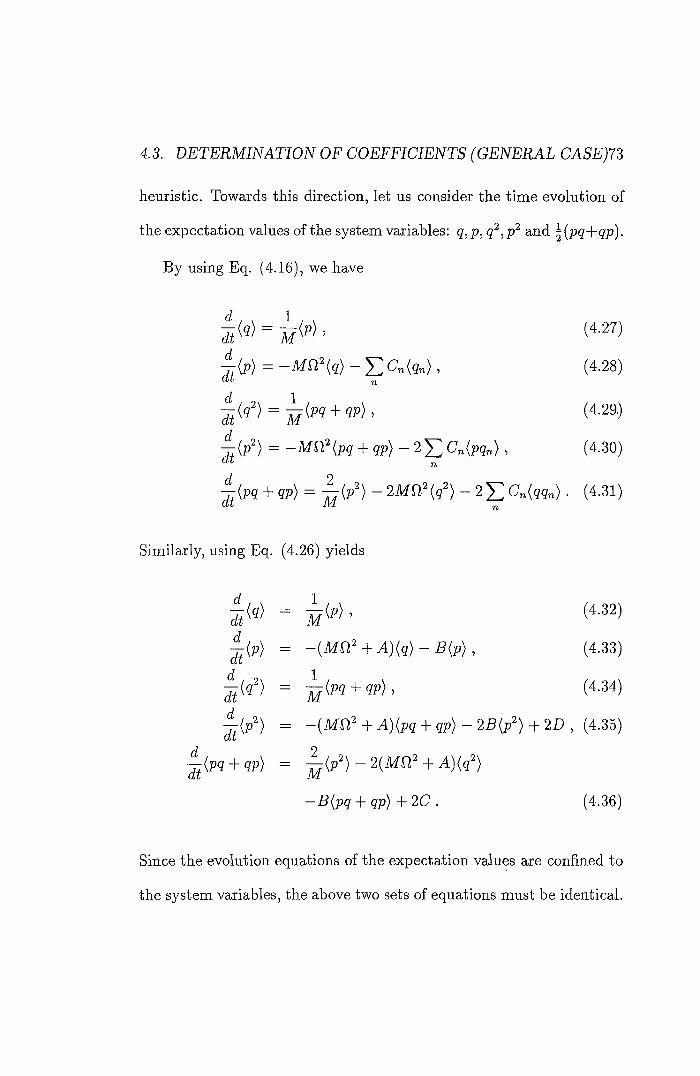
4.3. DETERMINATION OF COEFFICIENTS (GENERAL CASE)7$
heuristic. Towards this direction, let us consider the time evolution of
the expectation values of the system variables: g,p, and ^{pq+qp).
By using Eq. (4.16), we have
= —MVL {q) — ^Cn{qn) , (4.28)
, (4: S!9)
= -Mfl^{pq + qp) — 2'y]Cn{pqn) , (4.30)
— (pg + qp) — ~ 2MQ^(q^) — 2'^Cn{qqn) • (4.31)
Similarly, using Eq. (4.26) yields
(4.32)
= - ( M n ' + A ) ( g > - B ( p ) , (4.33)
== --(Jkfilf 4- yl)(f,g 4- ,%p) -- 4- SUD , (4.35)
4-<ZP) == -- -K /l)((r')
-B{pq + qp) + 20 . (4.36)
Since the evolution equations of the expectation values are confined to
the system variables, the above two sets of equations must be identical.
74 CHAPTER 4. QUANTUM BROWNIAN MOTION
Now by comparing (4.28) with (4.33) we see that
T,Cn{qr,) = A{q) + B{p) . (4.37)
Similarly, by comparing (4.31) with (4.36), (4.30) with (4.35), respec-
tively, we get
Cn{Q<ln) = + iriQP + PQ) — C , (4.38) n ^
Z) C'n(pgn) = ^ - (4.39) n ^
The coefficients A, B, C, D may now be determined from (4.37)-
(4.39) by regarding the expectation values (^), {(/„<?) etc. as expectation
values of Heisenberg picture operators, and by solving the operator
equation of motion. For simplicity, we still use ordinary notation to
represent an operator without adding a hat on it.
The solution to the equation of motion may be written
9»(^) — Pnp(i) y H" (0)) ; (4.40)
g( ) = a:g(0) + ^p(O) -K ^(ong»(0) + 6,iPn(0)) , (4.41) 71
for some time-dependent coefficients ck„, /3„, a„m, an-, K- Note
that qn{t) has been expressed in terms of the final, not initial values
of g,p. By substituting Eq. (4.40) into Eq. (4.37), keeping (4.11) in
mind, and comparing the two sides of the resulting equation, we have
A = ^ CnCKn , B ^ CnPn • (4.42)
4.3. DETERMINATION OF COEFFICIENTS (GENERAL CASE)75
Similarly, substituting (4.40) and (4.41) into (4.38) and (4.39), respec-
tively, we get
C = - I ] + 6nm6m(pl(0))) , (4.43)
D = - M ^ - (4.44) 77171
Here we have made use of p = Mq. The coefficients A, B, C, D are
therefore completely determined by solving the equation of motion.
We now do this explicitly.
We have
q(t) + Q.'^q{t) == ---TT Cnqn{t) , (4.45)
qn{t) + w^gn(^) = g(^) • (4.46) 171 n
The solution to Eq.(4.46) is as follows:
p„(0) sin(a;„^) (&i(Z) == gn(l])(X)8(Wn() 4"
777/^1. Wf]
Jo Un rUn
Combining (4.45) and (4.47) gives
2 J A, \ \ jf(f)
where
g( ) + n^g( ) + ^ ^ - 6)g(a) = — , (4.48)
f i t ) = (gn(0) cos(uj„t) + P"(Q) 8m(Wn<)\ ^ (4.49) n \ )
76 CHAPTER 4. QUANTUM BROWNIAN MOTION
The kernel i]{s) is defined as
7(5) = , (4.50)
where
r+co Kuj) 7 ( 5 ) = / du co8(wa) . (4.51)
Jo LO
Here I [u) is the spectral density of the environment:
/(w) = E <F(w - W » ) - ^ . (4.52)
In order to get the expressions (4.40) and (4.41), we solve equation
(4.48) with the following two different initial conditions:
q[s = 0) = g(0) , q{s = 0) = ^ . (4.53)
and
g(g = () = g(^) , g(g = () = ^ . (4.54)
where t is any given time point. In doing so, we consider the elementary
functions Ui{s){i = 1,2) introduced by Hu, Paz and Zhang [60] which
satisfy the following homogeneous integro-differential equation
2(a) + n"2(6) + ^ ( A,7(6 - A)2(A) = 0 (4.55)
with the boundary conditions:
ui{s = 0) = 1 , Ui(5 = t) = 0 , (4.56)
4.3. DETERMINATION OF COEFFICIENTS (GENERAL CASE)77
and
U2{s = 0) = 0 , U2{s = t) = 1 . (4.57)
The solution to equation (4.55) with the initial condition (4.53) is
obtained as the linear combination of
The solution to equation (4.48) with the homogeneous initial conditions
can be formally written as
^(5) = ^ T)/(T). (4.59)
Where Green function Gi{s^t) satisfies
ds^
with
7")+ ^^^^1(5, r ) + — F dXr](s~ X ) G I { X , T ) — S{S — T ) (4.60) M Jo
Gi{s = 0 , r ) = 0 , —Gi{s = 0,T) = 0 . (4.61)
Then the solution to the equation (4.48) with initial condition (4.53)
reads
q{s) = w{s)w{s)^ (4.62)
explicitly,
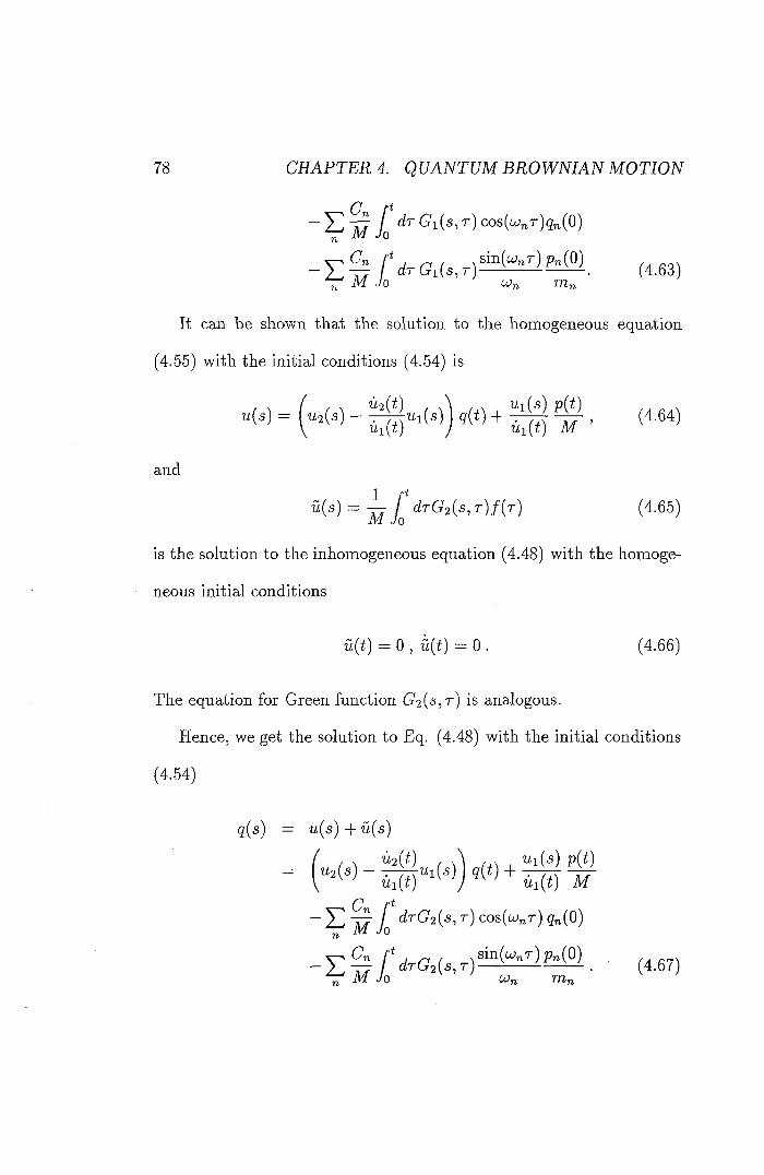
78 4 f%toi4/7vi/uv jVfo:rf()j\r
~12^ dTGi{s,T)cOs{(X>nT)qn{0)
(4.63)
It can be shown that the solution to the homogeneous equation
(4.55) with the initial conditions (4.54) is
+ i f )
and
(^TG2(g,T)/(7-) (4.65)
is the solution to the inhomogeneous equation (4.48) with the homoge-
neous initial conditions
{t(f) == 0 , {((0 == 0 . (4.66)
The equation for Green function r ) is analogous.
Hence, we get the solution to Eq. (4.48) with the initial conditions
(4.54)
q{s) = u{s) + u(5)
c/rG2(5,r)cos(u;„r)g„(0)
(4.67) ^ M Jo ^ ' UJn rUn ^ ^
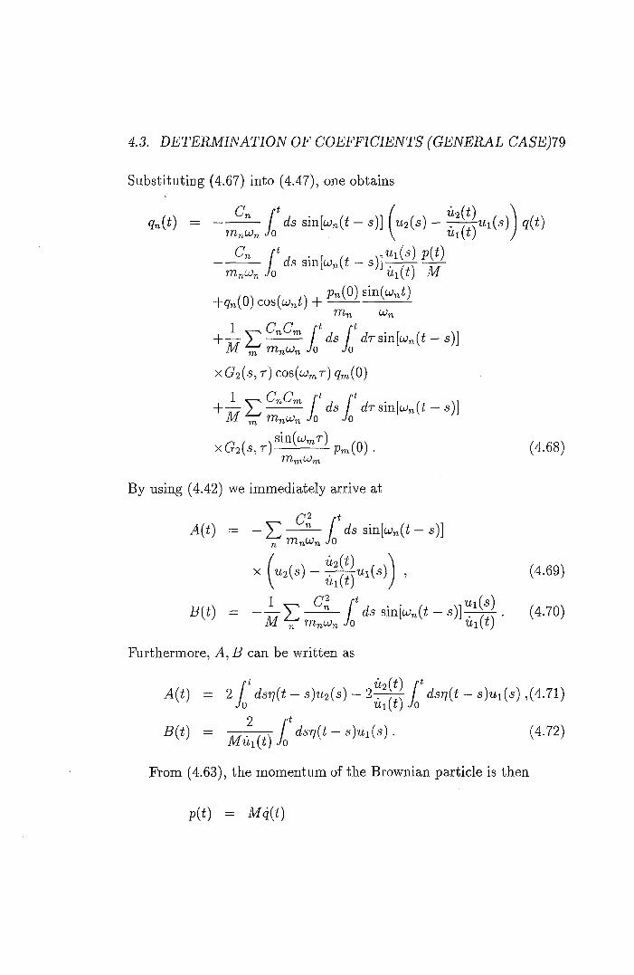
4.3. DETERMINATION OF COEFFICIENTS (GENERAL CASE)79
Substituting (4.67) into (4.47), one obtains
quit) = f ds sin[a;„(t - 5)] q{t)
f* , . r \i 1*1(4) P(0
+ , „ ( 0 ) c o 3 K i ) + P"(°'
' 'Vo
X(92(5, r ) C08(WmT) 9^(0)
X ( 9 2 ( 5 , 7 - ) ^ ^ ° ' ^ ^ " ' ^ ^ Pm{0) • (4.68) '^m^m
By using (4.42) we immediately arrive at
v4(z) = - y" —— f ds sin[a;„(t - 5)] t r rUnU^n Jo
X ^ t ( 2 ( g ) - - , ( 4 ( i s )
Furthermore, A, B can be written as
A{t) = 2 [ dsri{t — s)u2{s) — j dsr]{t — s)ui{s) ,{4:.71) Jo Ui[t) Jo
From (4.63), the momentum of the Brownian particle is then
]p(() == 7kfg(Z)
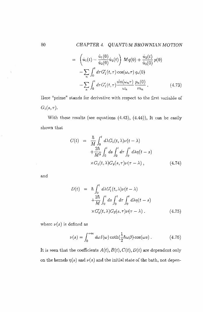
80 CHAPTER 4. QUANTUM BROWNIAN MOTION
f dTG[{t,T) COs{uJnT) qn{0) n "'O
- E (4,73) n -/O <^n rUn
Here "prime" stands for derivative with respect to the first variable of
Gi(6,T).
With these results (see equations (4.43), (4.44)), It can be easily
shown that
h
I Jo 2% f*
(/(Z) — Jq d.XGi{tj X)u{t — X)
M'£'''lo
and
xGi(t , A)G2('S,'r)z/(r - A) , (4.74)
D ( ^ ) = ^ y * ( i A G ; ( ( , A ) i / ( < - A )
2h y* ft
^mL ''"l ''^1'-*-''^
xG[{t,X)G2{s,T)u{r - X) . (4.75)
where u[s) is defined as
r+oo % i^{s) — J dujl{u) coth.(-hbj(3) cos{uis). (4.76)
It is seen that the coefficients A(f), -B(t), C(f), D{t) are dependent only
on the kernels ri(s) and u{s) and the initial state of the bath, not depen-
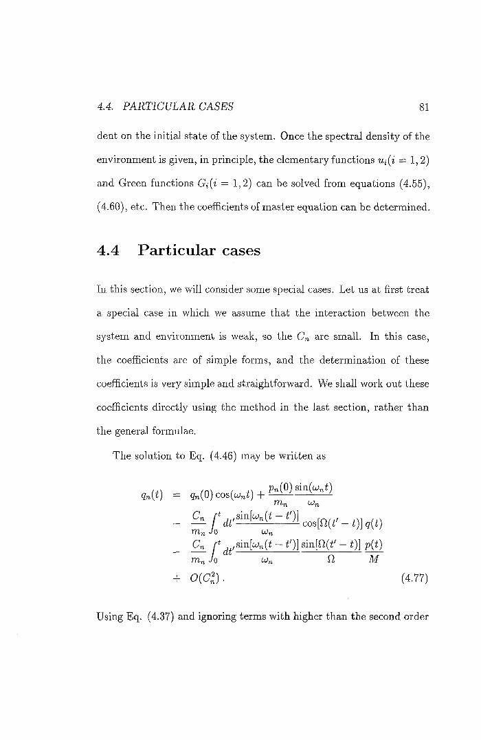
4.4. 81
dent on the initial state of the system. Once the spectral density of the
environment is given, in principle, the elementary functions Ui{i = 1,2)
and Green functions Gi{i = 1,2) can be solved from equations (4.55),
(4.60), etc. Then the coefficients of master equation can be determined.
4.4 P a r t i c u l a r cases
In this section, we will consider some special cases. Let us at first treat
a special case in which we assume that the interaction between the
system and environment is weak, so the C„ are small. In this case,
the coefficients are of simple forms, and the determination of these
coefficients is very simple and straightforward. We shall work out these
coefficients directly using the method in the last section, rather than
the general formulae.
The solution to Eq. (4.46) may be written as
«„(<) = +
Cn f* ,Sm[uJn{t-t')]
m„. Jo
Jo
Cn /•* ^^,8in[w»(( - f')] sin[0(f - it)] p{t)
rrin Jo UJn Q, M
+ 0(Cl). (4.77)
Using Eq. (4.37) and ignoring terms with higher than the second order
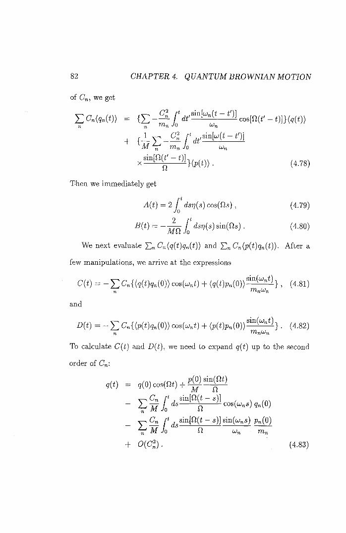
82 CHAPTER 4. QUANTUM BROWNIAN MOTION
of C„, we get
EC'M*)) = ( E / ' - i f ' c o s [ n ( f ' - i ) ] } ( g ( t ) )
M V rrinJo OJn
(4.78)
Then we immediately get
A(f) = 2 y dsr]{s) 003(^5) , (4.79)
^ 8in(ng). (4.80)
We next evaluate T.nCn{q{t)qn{t)) and T,nCn{p{t)qn{t))- After a
few manipulations, we arrive at the expressions
CM = - E C08(Wn() + (g( )Pn(0)) ^°^^^"^^} , (4.81) n
and
= - 1 ] C'»{(p(^)9n(0)) COs(Wn() + (p(()pn(0))^^^^^"^^} . (4.82) n '^TT-n^n
To calculate C{t) and D{t), we need to expand q(t) up to the second
order of C„:
q{t) = q{0) cos(m) +
- ^ cos(u;„5) g„(0)
Cn ^^sin[0(i - 5)] sin(cu„s) p„(0)
V M io „ ... n Wn m„
+ 0 ( c : ) . (4.83)
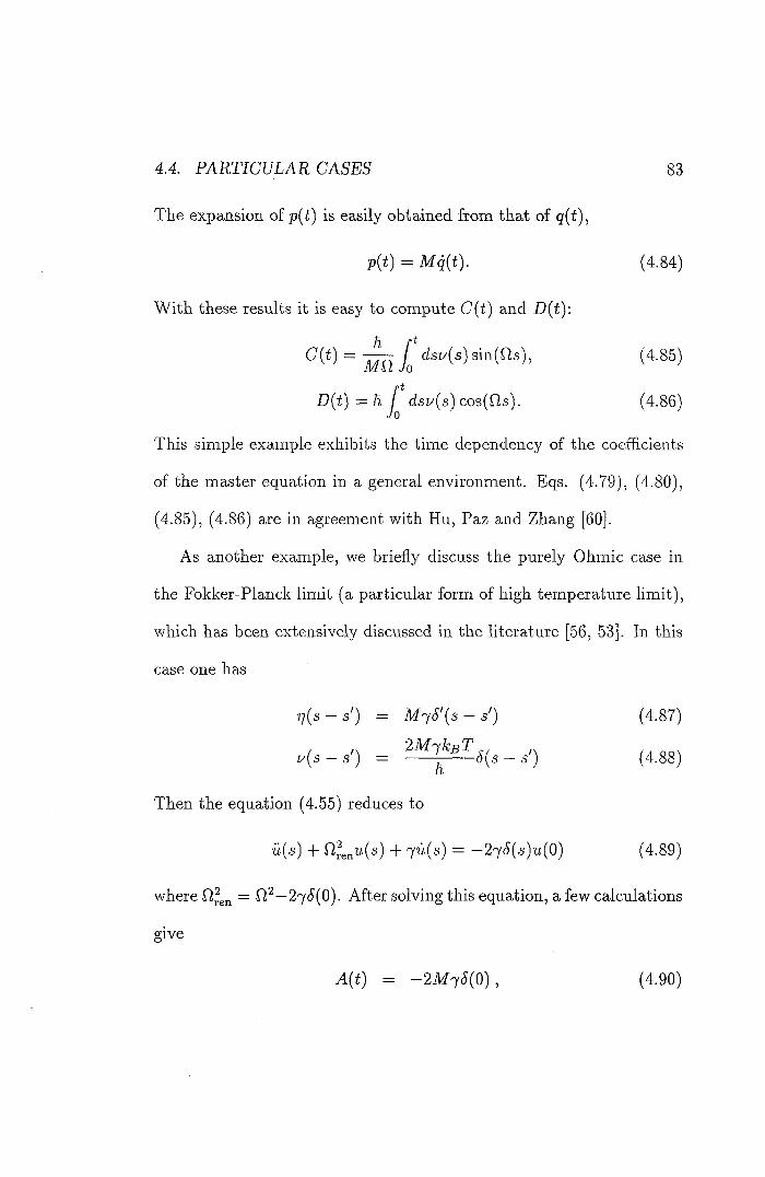
4L4. 83
The expansion of p(t) is easily obtained from that of q{t),
p{t) = Mq{t). (4.84)
With these results it is easy to compute C(t) and D{t):
^ ( 5i/(g) 8m(as), (4.85)
D{t)—h f (isi/(s) cos(Os). (4.86) Jo
This simple example exhibits the time dependency of the coefficients
of the master equation in a general environment. Eqs. (4.79), (4.80),
(4.85), (4.86) are in agreement with Hu, Paz and Zhang [60].
As another example, we briefly discuss the purely Ohmic case in
the Fokker-Planck limit (a particular form of high temperature limit),
which has been extensively discussed in the literature [56, 53]. In this
case one has
ri(s — s') — M'yS'{s — s') (4.87)
y ( a - g ' ) =
Then the equation (4.55) reduces to
u{s) + + 7^(5) = -27^(5)^^(0) (4.89)
where = 0^—27^(0). After solving this equation, a few calculations
give
A(() = -2M7(^(0), (4.90)
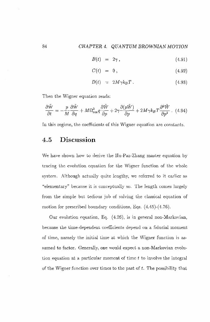
84 CHAPTER 4. QUANTUM BROWNIAN MOTION
= 2 ^ , (4.91)
== 0 , (4.92)
D{t) = 2M'ykjBT. (4.93)
Then the Wigner equation reads;
In this regime, the coefficients of this Wigner equation are constants.
4.5 Discussion
We have shown how to derive the Hu-Paz-Zhang master equation by
tracing the evolution equation for the Wigner function of the whole
system. Although actually quite lengthy, we referred to it earlier as
"elementary" because it is conceptually so. The length comes largely
from the simple but tedious job of solving the classical equation of
motion for prescribed boundary conditions, Eqs. (4.45)-(4.76).
Our evolution equation, Eq. (4.26), is in general non-Markovian,
because the time-dependent coefficients depend on a fiducial moment
of time, namely the initial time at which the Wigner function is as-
sumed to factor. Generally, one would expect a non-Markovian evolu-
tion equation at a particular moment of time t to involve the integral
of the Wigner function over times to the past of t. The possibility that
<L5. 85
this non-Markovian equation can be written in the simpler, superfi-
cially "memoryless" form (4.26) was first emphasised by Shibata et al.
[63,64,65].
Finally, we have a remark on the relevant work by Anglin and Habib
[66], who also consider the derivation of the Wigner equation Eq. (4.6)
by tracing the Wigner equation for the whole system. Their approach
is very similar to our derivation of Eq. (4.26) in section 4.2. They
also emphasised that, at least as far as solving equations goes, the
derivation is an essentially classical calculation. They do not, however,
give explicitly the detailed derivation of the coefficients, as we do in
section 4.3.
Chapter 5
Parameter-based Uncertainty Relations
"I have tasted eggs, certainly,"said Al-ice, who was a very truthful child; "but little girls eat eggs quite as much as ser-pents do, you know." "I don't believe it," said the Pigeon; "but if you do, why then they're a kind of serpent, that's all I can say."
—Lewis Carroll Alice's Adventures in Wonderland
5.1 I n t r o d u c t i o n
In [67] Mandelstam and Tamm prove the following uncertainty relation
between the time and energy:
\{ip{0)\tp{t))\'^ > cos^ [ ~ ~ ^ J ' (5.1) /A.Ht\ ^ ^ ^ Trfi
2 A 1
where AH = \/{H^} — {Sy. Since then the parameter based uncer-
tainty relation and related problems have been extensively studied in
86
,5.1 g?
various contexts [68, 69, 70, 71, 72, 73, 74, 75, 76, 77]. For an excellent
review, e.g. see [74].
The parameter-based uncertainty relations between position and
momentum has been considered in [71, 73]. A particular interesting
case can be formulated as follows: For a given state represented by
we use 8x to denote the distance for the translation of
to an orthogonal state and A P to denote the momentum uncertainty
in the state \'ip{x)), then
SxAP > ^ (5.2)
where h is Planck constant without being divided by 27r. The interpre-
tation of (5.2) may be as follows: The distance for displaced observer
who 'see' the quantum state is completely different from that the undis-
placed observer does is not less than AP/h. Note that this uncertainty
relation is on the same footing as that between time and energy (see
[70]).
In this chapter we shall provide a new derivation for the inequality
(5.2), we also prove that the right hand side of the above inequality (5.2)
can not be improved, namely, h/A is the greatest lower bound. Our
derivation is analogous to that in [76] for the time-energy uncertainty
relation.
88 CHAPTER 5. PARAMETER-BASED C/NCERTAfNTYRELATIONS
5.2 Der iva t ion of unce r t a in ty re la t ion
In the following, for simplicity, we only consider the wave functions
with one spatial dimension in the position space. Also, we assume that
the system is not in an eigenstate of the momentum operator P.
In order to get the shortest distance for the translation to an orthog-
onal state we introduce a formal quantity that will play a central role
in our derivation. This quantity is known as the correlation amplitude.
To begin with, let us consider a system in a state described by
the wave function (with a slight abuse of notation), we use the
notation — a)) to stand for the displaced state. The correlation
amplitude associated with these two states is defined as
C{a) = — a)) ( 5 . 3 )
The modulus of C{a) provides a quantitative measure of the "resem-
blance" between the states which are localised around different places,
or equivalently, the state remains unchanged but the observer is dis-
placed, then the above " between the states " should be replaced by "
between the observers ".
Our aim now is to find the smallest D which satisfies
C{D) — {\ip{x)\tj;'{x — D)) — Q. (5.4)
5.2. DERIVATION OF UNCERTAINTY RELATION 89
It is convenient to use (C(a)p. Taking the derivative with respect to
the parameter a then we get the following equation,
A da
|C(o)|" = 2Re - a)[il>(x)){i>(x)\^\<l>(x - a ) ) (5.5)
Let \ip{x — a)) be the state displaced through the distance a:
X — a)) = e (5.6)
It follows easily that
' ' 'x — a)) = ——P|'0(rc — a)) da
(5.7)
For any Hermitian operator A, the following formula holds [76, 78];
A|^(z)) = (A)l^(z)) + AA|T/'j.(2)> (5.8)
where
(A) = (T^(z)|A|TA(2))
AA = \/(A2> - (A>2
and |^(z)) and |'0j.(a;)) satisfy
(^(a;)|^j.(z)) = 0
Using (5.7) and (5.8), we obtain
^1^ (® - «)) = - «)) + AP\iP_l{X - a))] (5.9)
'^Note the decomposition on the right hand side of equality is not unique.
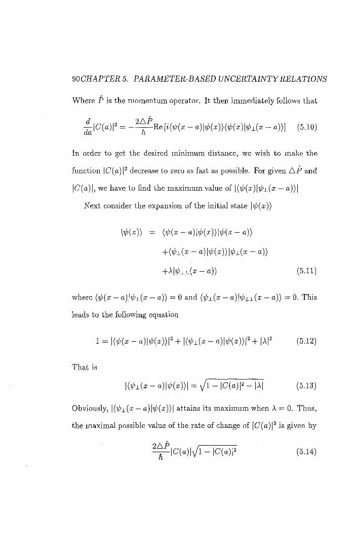
90CHAPTER5. PARAMETER-BASED UNCERTAINTY RELATIONS
Where P is the momentum operator. It then immediately follows that
^ | C ( a ) p = - a)\ip{x)){i^{x)\'tpx{x - a))] (5.10)
In order to get the desired minimum distance, we wish to make the
function |C(a)P decrease to zero as fast as possible. For given A P and
|C(a)|, we have to find the maximum value of — a))|
Next consider the expansion of the initial state [^(z))
+(^_L(z - - a))
+'^|'0j_x(^ — a)) (5.11)
where (^(a: — a)\tpx{x — a)} = 0 and (i/^±(x — a)lt/)j_±(x — a)) = 0. This
leads to the following equation
1 = j(^(x - a)l^(x)}l^ + - a)l^(x))j^ + |Ap (5.12)
That is
|(V'±(a: - o) |V'N)| = ] / l - |C(«)P - |A| (5.13)
Obviously, \{^^^±(x — a)\'tp(x))\ attains its maximum when A = 0. Thus,
the maximal possible value of the rate of change of |C(a)p is given by
2 A f , h
• | C ( o ) | ^ l - | C ( a ) | ^ (5.14)
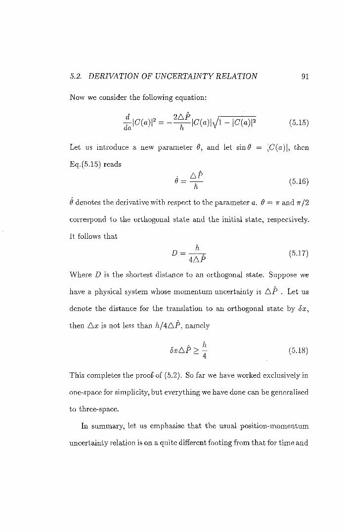
5.2. DERIVATION OF UNCERTAINTY RELATION 91
Now we consider the following equation:
l | C ( » ) p = - H | ^ | C ( « ) | y ' l - |C(a)P (5.15)
Let us introduce a new parameter and let sin0 = |C(o)|, then
Eq.(5.15) reads
A f g = — (5.16)
6 denotes the derivative with respect to the parameter a. 0 = -k and 7r/2
correspond to the orthogonal state and the initial state, respectively.
It follows that
D = (5.17) 4 A f
Where D is the shortest distance to an orthogonal state. Suppose we
have a physical system whose momentum uncertainty is A P . Let us
denote the distance for the translation to an orthogonal state by
then Ax is not less than A / 4 A f , namely
(^zAf > ^ (5.18)
This completes the proof of (5.2). So far we have worked exclusively in
one-space for simplicity, but everything we have done can be generalised
to three-space.
In summary, let us emphasise that the usual position-momentum
uncertainty relation is on a quite different footing from that for time and
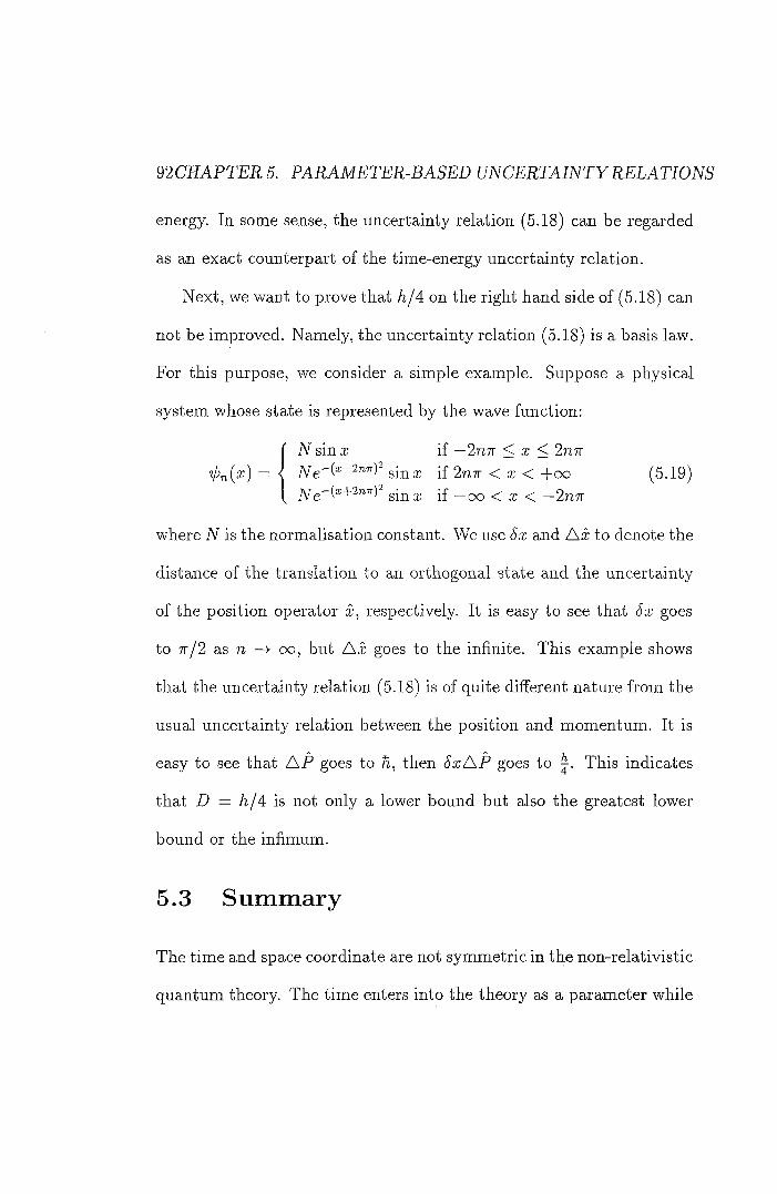
92 CEAf TEE 5. PARAMETER-BASED [/NCERTAfNTYREI/ATfONS
energy. In some sense, the uncertainty relation (5.18) can be regarded
as an exact counterpart of the time-energy uncertainty relation.
Next, we want to prove that A/4 on the right hand side of (5.18) can
not be improved. Namely, the uncertainty relation (5.18) is a basis law.
For this purpose, we consider a simple example. Suppose a physical
system whose state is represented by the wave function:
{ N sin X if —2?27r < x < 2n7r
]yg-(a;-2n7r)- if 2n7r < x < +00 (5.19) jYg-(a:+2nw)2 if —OO < X < —2n7r
where N is the normalisation constant. We use 5x and Ax to denote the
distance of the translation to an orthogonal state and the uncertainty
of the position operator x, respectively. It is easy to see that Sx goes
to 7r/2 as n —> oo, but Ax goes to the infinite. This example shows
that the uncertainty relation (5.18) is of quite different nature from the
usual uncertainty relation between the position and momentum. It is
easy to see that AP goes to then SxAP goes to This indicates
that D = A/4 is not only a lower bound but also the greatest lower
bound or the infimum.
5.3 S u m m a r y
The time and space coordinate are not symmetric in the non-relativistic
quantum theory. The time enters into the theory as a parameter while
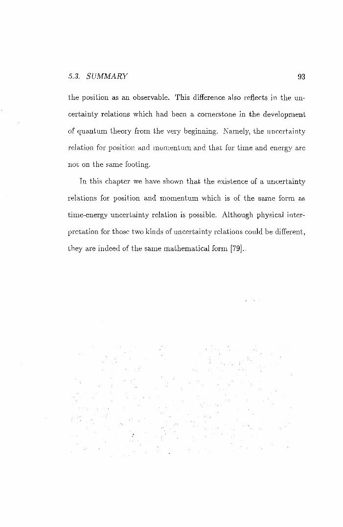
93
the position as an observable. This difference also reflects in the un-
certainty relations which had been a cornerstone in the development
of quantum theory from the very beginning. Namely, the uncertainty
relation for position and momentum and that for time and energy are
not on the same footing.
In this chapter we have shown that the existence of a uncertainty
relations for position and momentum which is of the same form as
time-energy uncertainty relation is possible. Although physical inter-
pretation for those two kinds of uncertainty relations could be different,
they are indeed of the same mathematical form [79].
Chapter 6
General Conclusion
The central themes of thesis are the investigation of various approaches
in connection to the quantum open systems and the foundations of
quantum theory.
We have discussed, based on a two-level system model, decoherent
histories approach, environment-induced decoherence and stochastic lo-
calisation of quantum jump simulation and quantum state diffusion.
We furnished a new derivation of master equation of QBM in general
environment, which is a typical quantum open system and is of partic-
ular importance in the recent advance of decoherence programmes.
In the last part of the thesis we have described a parameter-based
uncertainty relations for position and momentum.
We conclude the thesis with a remark. Recent advances in quan-
tum open system theory have opened up a brand new avenue of ex-
94
95
ploring the issues in quantum theory. Among others, the environment-
induced decoherence, decoherent histories, as well as various stochastic
Schrodinger equations have provided many important insights into the
solution to fundamental problems in quantum theory. However, the
power, depth and width of the new theories are far beyond fully ex-
plored and understood. It is very likely that what we have done so far
is merely one touch on the trunk of an elephant by a blind man, it is
still far to grasp the whole picture of the animal.
Appendix A
Proof of theorem
111 t h i s A p p e n d i x , w e s h a l l g i v e a p r o o f o f T h e o r e m i n C h a p t e r I I . S i n c e
b o t h M a n d N a r e p o s i t i v e d e f i n i t e m a t r i c e s , t h e r e f o r e , o n e o f t h e m ,
s a y , N c a n b e d e c o m p o s e d a s
yy = (/L.i)
w h e r e S i s a n n x n m a t r i x . A f t e r a n a r r a n g e m e n t , t h e r i g h t - h a n d s i d e
o f E q . ( 2 . 5 0 ) b e c o m e s
|Tr ( M f I = |Tr |. (A.2)
S u p p o s e X m a r e a n o r t h o n o r m a l b a s i s i n n d i m e n s i o n a l s p a c e V . T h e n
|Tr ( M f ATQ) I = I 771
w h e r e i s t h e t r a n s p o s e o f X m - N o w , w e s e t
Vm — QS^Xmt ( A . 4 )
= P S ^ X m - ( A . 5 )
96
97
Then the trace in Eq. (A.3) may be rewritten as
= (A.6) m
Since Hm, are orthogonal vectors and M is a positive definite matrix,
then it is not difficult to arrive at the following inequality (see [80])
I I < , (A.7)
where and are the largest
and the smallest eigenvalues of M, respectively. Combining (A.7) with
Cauchy's inequality,
( E < Z Z (A.8) m m m
then (A.3) becomes
]Tr (MPJV0)1 = (sOMPS't):c„|
< Y,\ymMZm\ m
< (A.9) m m
It is easy to identify that
Ti(MPNP) = Y.ylMy^, (A.IO) m
Tr(MQ^Q) = (A. l l )
98 APPENDIX A. PROOF OF THEOREM
This proves that
|Tr ( M f I < [Tr (MPTVf [Tr ( M Q . (A.12)
Since M and N are in the completely symmetric position, so the similar
result is true for . Then it completes the proof of the theorem. •
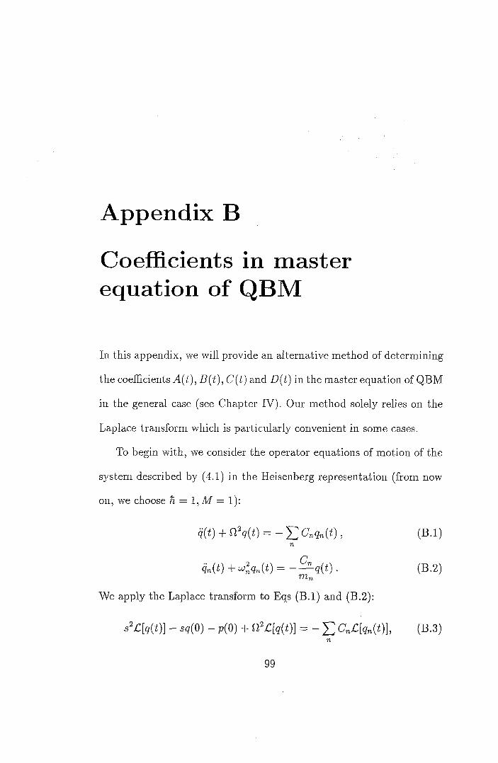
Appendix B
Coefficients in master equation of QBM
In this appendix, we will provide an alternative method of determining
the coefficients A(t), B{t)^ C{t) and D{t) in the master equation of QBM
in the general case (see Chapter IV). Our method solely relies on the
Laplace transform which is particularly convenient in some cases.
To begin with, we consider the operator equations of motion of the
system described by (4.1) in the Heisenberg representation (from now
on, we choose /i = 1, M = 1):
g(<) + , (B.l)
^n{t) — g(^) • (B.2)
We apply the Laplace transform to Eqs (B.l) and (B.2);
s^C[q{t)] — 5^(0) — p(0) + Q?C[q{t)] — — ^ CnC[qn{t)], (B.3)
99
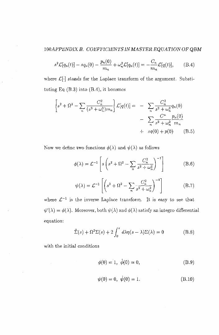
m APPENDIX B. COEFFICIENTS IN MASTER EQ UATION OF QBM
Pn(0) a ^[?n(^)] — •59n(0) H — (B.4)
rUr
where £[•] stands for the Laplace transform of the argument. Substi-
tuting Eq (B.3) into (B.4), it becomes
5 + 9? E n + ^ 4
- E C" Pn(0)
+ 69(0)+p(0) (B.5)
Now we define two functions < (A) and ^(A) as follows
( (A) = r -1 c ' -1
'0(A) = C -1 r ^2
(B.6)
(13.7)
where is the inverse Laplace transform. It is easy to see that
'0'(A) = ^(A). Moreover, both and 0(A) satisfy an integro-difFerential
equation:
2(5) + O^S(a) + 2 ^,7(6 - A)S(A) = 0 (B.8)
with the initial conditions
0(0) = 1, 0(0) = 0,
V'(O) = 0, ^(0) = 1.
(B.9)
(B.IO)
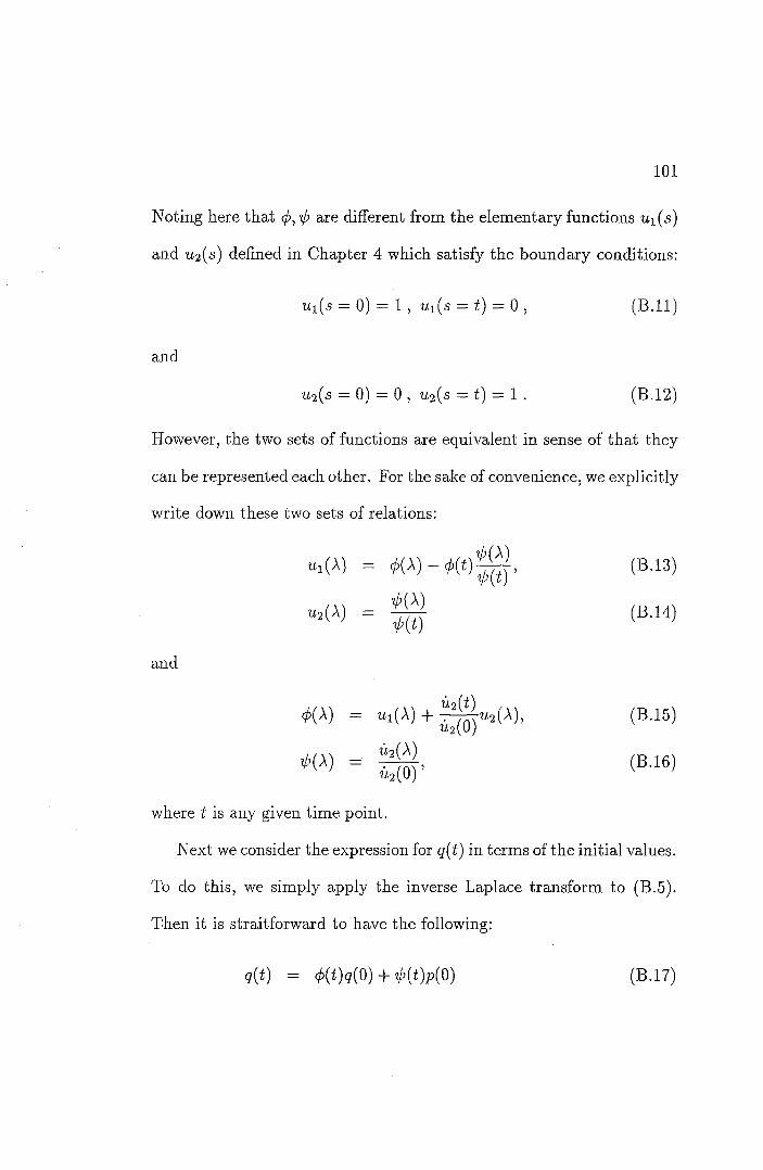
101
Noting here that ( , xjj are different from the elementary functions «i(g)
and ^2(5) defined in Chapter 4 which satisfy the boundary conditions:
ui(s = 0) = 1 , ui(5 = t) = 0 , (B.l l )
and
U2{s = 0) = 0 , 1(2(5 = t) = 1 . (B.12)
However, the two sets of functions are equivalent in sense of that they
can be represented each other. For the sake of convenience, we explicitly
write down these two sets of relations:
«.(A) = (B.13)
- g and
0(A) = ui(A) + (B.15)
where t is any given time point.
Next we consider the expression for q{t) in terms of the initial values.
To do this, we simply apply the inverse Laplace transform to (B.5).
Then it is straitforward to have the following:
g(f) = <^(t)g(0) + ^(t)p(0) (B.17)
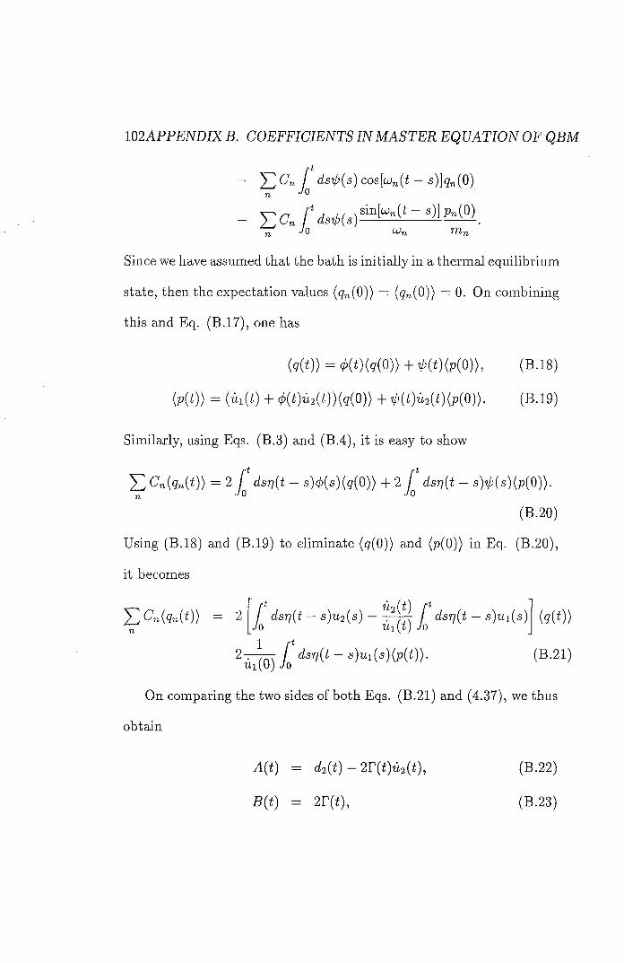
102 APPENDIX B. COEFFICIENTS IN MASTER EQ UATION OF QBM
dsip{s) COs[uJn{t - S)]qn(0)
- E C .
Since we have assumed that the bath is initially in a thermal equilibrium
state, then the expectation values (<2'n(0)) = (<?n(0) ) = 0. On combining
this and Eq. (B.17), one has
= <^(()(g(0)) + ^(^)(X0)), (B.18)
(p(()) = (i[i(() + (^(^)t[2(())(g(0)) + ^(()t(2(^)(p(0))- (B.19)
Similarly, using Eqs. (B.3) and (B.4), it is easy to show
^ - -s)4a)(g(0)> + 2 / d577(t - a)^(5)(p(0)>.
(B.20)
Using (B.18) and (B.19) to eliminate (g(0)) and (p(0)) in Eq. (B.20),
it becomes
]^Gn(g,:(^)) = 2 I dsi]{t - s)u2{s) - . / dsri{t - s)ui{s 0 Ui[t) Jo
2 1 '•
(gW)
j dsri{t — s)ui{s){p{t)). (B.21) 1^1(0)
On comparing the two sides of both Eqs. (B.21) and (4.37), we thus
obtain
A(<) = (f2(<)-2r(<)u3((), (B.22)
B(() = 2r(<), (B.23)
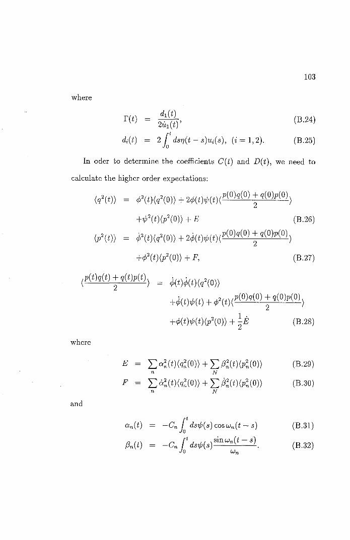
103
where
" W = # ' (S.24)
di{t) = 2 ^ dsr]{t - s)ui{s), (z = 1,2). (B.25)
In oder to determine the coefficients C{t) and D{t), we need to
calculate the higher order expectations:
+^"(^)(p"(0)) + E (B.26)
{/{()) = ^=(t)(g'(O)> + 2 0 ( o ^ ( < ) ( ? ^ M ? ) + i ( 2 M )
+#(i ) (p'(0)) + F, (B.27)
+«i)V,(i) + ^ ^ ( i ) ( ? 2 M 2 ) + i ( 2 M 2 ) )
+4>{i)4>{i){p^{0)) + -E (B.28)
where
and
E = (B.29) n N
F = E«»{ ' ) (9 ' ( 0 ) ) + E/5n(')(Pn(»)) (B.30) n J\f
(Xn{t) = -Cn dsip{s) COS OJn{t — s) (B.31)
(B.32) 0 CUvi
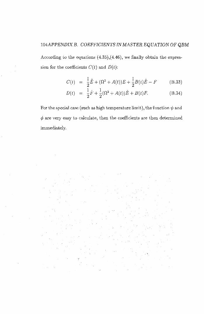
104APPENDIX B. COEFFZCJENTS IN MASTER EQUATION OF QBM
According to the equations (4.35),(4.46), we finally obtain the expres-
sion for the coefficients C{t) and D{t):
C(f) = ^E + (n" + A ( ^ ) ) E + ^ B ( < ) E - F (B.33)
D(() = l F + l (n" + A(^))E + B(t)F. (B.34)
For the special case (such as high temperature limit), the function ijj and
(f) are very easy to calculate, then the coefficients are then determined
immediately.
Bibliography
[1] Quantum Theory and Measurement., edited by J.A. Wheeler and
W.H. Zurek (Princeton University Press, Princeton, NJ, 1983).
[2] W.H. Zurek, Phys. Rev. D 24, 1516 (1981); Phys. Rev. D 26, 1862
(1982).
[3] W.H. Zurek, Phys. Today 44 (10), 36 (1991).
[4] W.H. Zurek, Prog. Theor. Phys. 89, 281 (1993) and references
therein; and in The Physical Origins of Time Asymmetry, edited
by J.J. Halliwell, J. Perez-Mercader and W. Zurek (Cambridge Uni-
versity Press, Cambridge, England, 1994).
[5] R.B. Griffiths, J. Stat. Phys. 36, 219 (1984).
[6] R. Omnes, J. Stat. Phys. 53, 893 (1988); J. Stat. Phys. 53, 933
(1988); J. SW. Piiys. 53, 957 (1988); J. SW. Phys. 57, 357 (1989);
Rev. Mod. Phys. 64, 339 (1992).
105
106 BfBLfOGRAPHY
[7] R. Omnes, The Interpretation of Quantum Mechanics (Princeton
University Press, Princeton, New Jersey, 1994).
[8] M. Gell-Mann and J. Hartle, in Complexity, Entropy, and the
Physics of Information, SFI Studies in the Science of Complexity,
Vol. VIII," edited by W. Zurek (Addison Wesley, Reading, USA,
19M).
[9] M. Gell-Mann and J. Hartle, Phys. Rev. D 47, 3345 (1993).
[10] J. Hartle, in Quantum Cosmology and Baby Universe, edited by
S. Coleman, J. Hartle, T. Piran, and S Weinberg (World Scientific,
Singapore, 1991).
[11] N. Gisin and I.C. Percival, J. Phys. A 25, 5677 (1992); J. Phys.
A 26, 2233 (1993); J. Piys. A 26, 5677 (1993).
[12] H.J. Carmicliael, An Open Systems Approach to Quantum Optics
(Springer-Verlag, Berlin, 1994).
[13] H.M. Wiseman and G.J. Milburn, Phys. Rev. A 47, 1652 (1993).
[14] L. Diosi, J. Piys. A 21, 2885 (1988).
[15] I. Percival, J. Phys. A 27, 1003 (1994).
BIBLIOGRAPHY 107
[16] N. Gisin, P.L. Knight, I.C. Percival, R.C. Thompson and D.C.
Wilson, J. Mod. Optics, 40, 1663 (1993).
[17] B. Garraway and P.L. Knight, Phys. Rev. A 49, 1266 (1994).
[18] L. Diosi, N. Gisin, J. Halliwell and I. Percival, Phys. Rev. Lett.
74,203 (1995).
[19] J. Halliwell and A. Zoupas, Phys. Rev. D 52, 7294 (1995).
[20] T. Yu, PAygjca A 248, 393 (1998).
[21] J. Halliwell and T. Yu, Phys. Rev. D 53, 2012 (1996).
[22] T. Yu, P6yg. lett . A 223, 9 (1996).
[23] H.D. Zeh, Found. Phys. 1, 69 (1971).
[24] E. Joos and H.D. Zeh, Z.Phys. B 59, 223 (1985).
[25] J.B. Paz, S. Habib, and W.H. Zurek, Phys. Rev. D 45, 2843 (1992)
[26] W.H. Zurek, S. Habib, and J.B. Paz, Phys. Rev. Lett. 70, 1187
(1993)
[27] J. B. Paz and W. H. Zurek, Phys. Rev. D 48, 2728 (1992).
108 BIBLIOGRAPHY
[28] J.J. Halliwell, "A Review of the Decoherent Histories Approach
to Quantum Mechanics", in proceedings of the Baltimore con-
ference, Fundamental Problems in Quantum Theory, edited by
D.Greenberger (New York Academy of Sciences New York, New
York, 1995).
[29] J.B. Hartle, Spacetime Quantum Mechanics and the Quantum
Mechanics of Spacetime in Proceedings of the 1992 Les Houches
Summer School, Gravitation et Quantifications, edited by B.Julia
(North-Holland, 1995).
[30] H.F. Dowker and J.J. H alii well, Phys.Rev. D 46, 1580 (1992).
[31] C. Isham, J. Math. Phys. 35, 2157 (1994).
[32] C. Isham and N. Linden, J. Math. Phys. 35, 5452 (1994).
[33] S. Goldstein and D. Page, Phys. Rev. Lett. 47, 3715 (1995).
[34] R. Laflamme and A. Matacz, Int. J. Mod. Phys. D 48, 171 (1993).
[35] J. Twamley, Phys. Rev. D 48, 5730 (1993).
[36] J. Finkelstein, Phys. Rev. D 47, 2843 (1993).
[37] C.G. Gardiner, Quantum Noise (Springer-Verlag, Berlin, 1994).
BIBLIOGRAPHY 109
[38] D.F. Walls and G.J. Milburn, Quantum Optics (Springer-Verlag,
Berlin, 1994).
[39] J.J. Halliwell and A. Zoupas, Pbys. Rev. D 55, 4697 (1997).
[40] J. N. McElwaine, Phys. Rev. A 53, 2021 (1996).
[41] M. Gallis, Pbys. Rev. A 53, 655 (1996).
[42] G. Lindblad, Comm. Math. Pbys. 48, 119 (1976).
[43] L. Diosi and W. Strunz, Phys. Lett. A 235, 569 (1997).
[44] L. Diosi, N. Gisin and W. Strunz, Non-Markovia,n Qua,ntum State
Diffusion, preprint 1998, quant-ph/9803062 (unpublished).
[45] C. W. Gardiner, A Handbook of Stochastic Methods (Springer,
Berlin, 1985).
[46] R. Schack, T. Brun and 1. Percival, Quantum State Diffusion, Lo-
calisation and Computation. ~J, A 2 - S A - ^ f
O M R S ' ) .
[47] T.Brun, N. Gisin, P. O'Mahony and M. Rigo, From Quan-
tum Trajectories to Classical Orbits, A ^ ^
110 BIBLIOGRAPHY
[48] T. Bmn, Phys. Rev. Lett. 78. 1833 (1997).
[49] M. Plenio and P. Knight, Rev. Mod. Phys. 70, 101 (1998).
[50] G.S. Agarwal, Phys. Rev. A 3, 828 (1971); Phys. Rev. A 4, 739
(1971); H. Dekker, Phys. Rev. A 16, 2116 (1977); Phys.Rep. 80,
1 (1991); G.W. Ford, M. Kac and P. Mazur, J. Math. Phys. 6,
504 (1965); H. Grabert, P. Schramm, G-L. Ingold, Phys. Rep. 168,
115 (1988); V. Hakim and V. Ambegaokar, Phys. Rev. A 32, 423
(1985); J. Schwinger, J. Math. Phys. 2, 407 (1961); I.R. Senitzky,
Phys. Rev. 119, 670 (1960).
[51] R. Kubo, M. Toda, N. Hashitsume, Statistical Physics (Springer,
Berlin, 1985).
[52] C. Anastopoulos and J.J. Halliwell, Phys. Rev. D 51, 6870 (1995).
[53] B.L. Hu and Y. Zhang, Mod. Phys. Lett. A 8, 3575 (1993).
[54] W. Zurek, in Proceedings of the NATO Advanced Study Institute
on Non-Equilibrium Statistical Mechanics, Sante Fe, 1984 (Plenum,
New York, 1984).
[55] W.G. Unruh and W. Zurek, Phys. Rev. D 40, 1071 (1989).
[56] A.O. Caldeira and A.J. Leggett, Physica A 121, 587 (1983).
BIBLIOGRAPHY 111
[57] H. Dekker, Phys. Rev. A 16, 2116 (1977).
[58] F. Haake and R. Reibold, Phys. Rev. A 32, 2462 (1985).
[59] J.P. Paz, in The Physical Origins of Time Asymmetry, edited by
J.J. Halliwell, J. Perez-Mercader, and W. Zurek (Cambridge Uni-
versity Press, Cambridge, 1994).
[60] B.L. Hu, J. Paz, and Y. Zhang, Phys. Rev. D 45, 2843 (1992).
[61] B.L. Hu, J. Paz, and Y. Zhang, Phys. Rev. D 47, 1576 (1993).
[62] N. Balazs and B.K. Jennings, Phys. Rep. 104, 347 (1984);
M.Hillery, R.F.O'Connell, M.O.Scully and E.P.Wigner, Phys. Rep.
106, 121 (1984); V.I.Tatarskii, Sov. Phys. Usp. 26, 311 (1983).
[63] N. Hashitsume, F. Shibata, and M. Shingu, J. Stat. Phys. 17, 155
(1977).
[64] F. Shibata, Y. Takahashi, and N. Hashitsume, J. Stat. Phys. 17,
177 (1977).
S. Chaturvedi and F. Shibata, Z. Physik B 35, 297 (1979).
[66] J. Anglin and S. Habib, Mod. Phys. Lett. A 11, 2655 (1996).
[67] L. Mandelstam and I. Tamm, J. Phys. (USSR) 9, 249 (1945).
112 BIBLIOGRAPHY
[68] G.N. Fleming, Nuovo Cimento A 16, 263 (1973).
[69] K. Bhattacharyya, J. Phys. A 16, 2993 (1983).
[70] J. Uffink and J. Hilgevoord, Found. Phys. 15, 925 (1985).
[71] J. UfSnk, Phys. Lett. A 108, 59 (1985).
[72] J.M. Levy-Leblond, Phys. Lett. A 111, 353 (1985).
[73] J. Hilgevoord and J. Uffink, in Microphysical Reality and Quantum
Formalism., edited by A. van der Merwe et al. (Kluwer, Dordrecht,
1988).
[74] J. Hilgevoord and J. Uffink, in Sixty-two years of Uncertainty,
edited by A. Miller, (Plenum, N.Y., 1990) and references therein.
[75] J. Anandan and Y. Aharonov, Phys. Rev. Lett. 65, 1697 (1991).
[76] L. Vaidman, Am. J. Phys. 60, 182 (1992).
[77] J. Uffink, Am. J. Phys. 61, 935 (1993).
[78] Y. Aharonov and L. Vaidman, Phys. Rev. A 41, 11 (1990).
[79] L. Vaidman and 0 . Belkind, Phys. Rev. A 57, 1583 (1998).
[80] B. Meister, PhD Thesis, Imperial College 1996, (unpublished).