Applying Resource Loading, Production & Learning Curves to ...

AEW Services, Vancouver, BC ©2001 Email: [email protected]

Applying Resource Loading, Production & Learning Curvesto Construction: A Pragmatic Approach

This paper was first published in the Canadian Journal of Civil Engineering, Vol. 21, 1994pp 939-953, under the title "A Pragmatic Approach to Using Resource Loading, Productionand Learning Curves on Construction Projects".

Abstract

The purpose of this paper is to present some rules of thumb based on experience for theearly planning of new civil and building construction work. In such construction, resourceinput (men, materials, equipment, etc.) is varied according to the planned timing andavailability of the work. On a well-run site, this resource loading as well as its consequentoutput follows a distinctive pattern within relatively narrow limits for the whole of the job.Practical considerations why this should be so are presented.

Based on experience, this paper suggests first approximation profiles for both typicalresource loading and progress S-curves, and shows that the difference could be due to theeffects of learning. The basis for calculating the shape of the learning curve and how theapplication of this concept is limited on a construction site are described. The manner inwhich an alternative learning curve calculation can be more useful in tracking progress isdemonstrated. The significance of these profiles and their relationships for improvedplanning and tracking of new construction work is suggested. An example of the outputfrom a less-well managed project as compared to the planned S-curve is also included.

Keywords: learning curve, productivity improvement, progress/production curve,resource loading.

Introduction

In order to optimize productivity on new facility construction, the input of resourcesincluding men, materials and equipment, is varied according to the planned timing andavailability of the work. This applies on all but the smallest construction jobs whereminimal crew size may limit flexibility. However, even on quite small “maintenanceprojects" this flexibility may be facilitated by managing the manpower levels over severalconcurrent assignments. This optimizing of productivity results in an initial period of buildup, a period of peak loading, followed by a period of progressive demobilizing. This typicalprofile, or curve, when plotted cumulatively over time for a whole project, results inanother typical curve in the shape of the letter “S”.

The purpose of this paper is to present some rules of thumb relating to these curveswhich have resulted from experience on new civil and building construction work. Theserules of thumb suggest simple ways to draw first approximations for cumulative resourceor production curves over the life of the project. The first relates to resource loading, i.e.men, materials, equipment or cash. A second relates to the consequent production output.The two curves are closely related and it is suggested that the difference can beaccounted for by the effects of learning. The phenomenon of learning itself is alsoexplored to show how it may be used for planning or tracking repetitive tasks onconstruction work.

These relationships have been found by the author to be most helpful for preliminary

Resource Loading, Production & Learning Curves in Construction of 26

AEW Services, Vancouver, BC © 2001 Email: [email protected]

project planning, for checking the validity of proposed plans, or for analyzing the recordsof completed work. Since the author has used these techniques while employed variouslyby owners, developers, and general contractors, it is hoped that they will be seen asbeneficial for anyone in similar positions.

In the following discussion, unless otherwise stated, the presumption is that the project isor will be “well run”. For the definition of a well-run construction job, refer to Appendix 1.

Resource Loading (input)

Figure 1 shows an example of manpower loading for a profitable civil contract which waspredominantly formwork and concrete placing.1 It displays a histogram of the make upand total numbers in the production work force, week by week over a 38 week period. Italso shows the progressive cumulative total, or actual manpower loading S-curve. Asnoted earlier, the general profiles of these curves appear to be quite typical (Christian1991) whether the observations refer to a whole construction project, a sub-contract, anindividual trade or a continuous construction activity of significant duration.

Figure 1 – Civil contract example of site manpower (predominantly) concretework

The important points to note about the S-curve are that the initial part of the curverepresents the "build-up", the central part of the curve is relatively "steady-state", oreffectively a straight line slope, and the latter part of the curve represents a "run-down"which closely mirror-images the early part of the S-curve.

In order to understand the generality of the suggested rules of thumb that follow, it isinstructive to recite the many practical reasons for the shapes of each of these threestages.

1 From the author’s personal records of progress tracking.



In Stage 1 there is an accelerating build up of manpower because

§ Access to the work has to be opened up from a zero start, with the result that thework itself becomes progressively more available.

§ Necessary preliminary preparatory activities, including planning and understandinglocal conditions, as well as ordering of materials, etc., often require fewer peoplebut more intensive supervision.

§ Key people may be brought in to start the work, but supporting labour is recruitedlocally. The recruiting and selection of local labour itself takes time.

§ With productive efficiency in mind, crews are added only as experience builds andthe work becomes available to be performed.

§ Further crews are added only as pressure builds to get the job done within therequired time frame.

Stage 2 achieves a steady state because

§ The working environment has reached optimum conditions for balancedperformance and repetition.

§ Physical limitations to the capabilities of the men and equipment provided isreached.

§ Adding more labour or separate crews would over-crowd the working area andreduce productivity.

§ The number of repetitions available from which the benefits of "productivityimprovement" can be derived would be reduced.

§ In either case the costs would be higher.§ Alternatively, if the work force is held at a lower level, the elapsed time to

accomplish the work will be prolonged, with consequent higher overheads and,possibly, contract penalties to be faced.

These obvious trade-offs require careful management and balance.

In stage 3 almost the reverse of Stage 1 is true. Manpower is progressivelyreduced because

§ The work begins to run out.§ The remaining work space not occupied by following trades, or owner occupation,

runs the danger of becoming over crowded.§ Morale sometimes deteriorates as the end of the work is in sight and people leave

to join more active sites§ Less successful crews or individuals are let go first.§ The more difficult work may have been left to the end, may be more congested, or

otherwise require only the skills of those brought in initially.§ Pressure to complete "the last few percent" dies down as management attention

turns to more critical work.§ Latent defects may surface upon final inspection requiring re-work with no added

measurable product to show for the effort.

A report issued by the National Electrical Contractors Association (NECA) in 1983 furtherillustrates the general shape of the resource loading S-curve. Data was collected from 40different contractors on 54 building projects in 32 cities. The projects represented fourbroad types of public buildings competitively bid and which the contractors felt were



typical of their business. The report includes the supporting data which show the ranges ofvariation.

Figure 2 shows the overall average manpower consumption rate S-curve for all the datacollected (NECA 1983). The figure also shows the overall low and high values and it isinteresting to note that the range of variation over a considerable number of projects isonly 10% of the total time scale. It should also be noted that a particular conditiontypically prevails in electrical work on building construction. At the outset, only a smallcrew is required for installing conduit and other electrical hardware during the course ofwork by other trades. The bulk of the electrical work cannot be undertaken until thosetrades are substantially complete. In other words, the work takes longer to open up andaccounts for a longer Stage 1 in this particular S-curve.

Figure 2 – Cumulative manpower consumed for electrical systems installationin new buildings — NECA

Progress S-curves (output)

As might be expected, the foregoing factors have a considerable impact on totalproduction especially as represented by the more familiar output or progress S-curves.

A complete determination of the project status and projections to final completion formanagement action can perhaps best be tracked by an integrated cost/schedule systemor technique known as "Earned Value and Performance Measurement" (Kerzner 1989).The earned value, i.e. the Budgeted Cost of Work Performed (BCWP), is determined atregular intervals during the course of the project. At the same time, the Actual Cost ofWork Performed (ACWP) is also determined, and both are compared to the baseline planwhich is the Budgeted Cost of Work Scheduled (BCWS). By presenting these resultsgraphically as S-curves, the variances in cost and schedule can readily be seen, and byanalyzing the results relative to the baseline plan S-curve, estimates can be made ofanticipated variations at completion. The key elements of the technique are shown in



Figure 3.

Figure 3 – Earned value and performance measurement

The technique is especially useful on projects involving a large number of significantactivities by different trades and/or under conditions which change during the course ofthe work. There are, however, several weaknesses in the approach (Meredith 1985). Costdata must be collected which reflects the actual progress of the work, work in progressmust be measurable and it must be measured. Consequently, this form of trackingrequires significant additional effort or qualified dedicated staff to collect reasonablyreliable data. This is particularly true where large purchases of off-site equipment mayinvolve staged payment assessments.

Since the results are at best estimates of work-in-hand and the final results are estimatedprojections, the technique is not usually considered worth the effort on most projects. Theexceptions are large complex projects, or projects on which this approach is requiredunder the terms of the contract. When the technique is adopted, an essential element inits successful use is a realistically shaped baseline plan S-curve.

A better strategy for tracking progress is to identify the major critical activities on site thatare measurable and plot those S-curves as surrogates for the whole job or stages of thejob. Figure 4 shows three S-curves2 illustrating different major activities. To facilitatecomparison they are shown plotted as percent progress against percent time.

Curve (a) shows progress on a 5560 pipe pile driving contract lasting 137 working days.Curve (b) shows the cumulative progress on a 180,000 cu. yd. bulk excavation contractlasting 15 weeks. Notice the progressive addition of plant as the work opens up in thebeginning, and the subsequent removal of plant as the availability of work runs out

2 From the author’s personal records of progress tracking.



towards the end. Curve (c) shows progress on a 7-month civil contract as reflected by theapproved monthly measurement progress billings.

Figure 4 – Three examples of progress S-curves

Figure 5 – Placing of formed structural concrete.Total concrete = 31 900 m3; total time = 16.5 months

Figure 5 shows measured progress on a 42,000 cu. yd. structural concrete activity of 16-months duration in Ontario, Canada. This curve is interesting because it clearly shows the



slow down in progress over the winter months. The original data indicates that the virtualcessation of activities due to cold weather was only two-and-a-half months. However, dueto the S-curve effects just before and after the cold weather cessation, the total impact ofthis condition was closer to three-and-a-half months. In the preparation of the originalconstruction schedule, this situation could have been reasonably foreseen and anappropriate adjustment made to the "standard" S-curve profile. What can be Learned ofPractical Value?

Manpower Consumption

In Figure 6, the data in Figure 1 has been re-plotted to a horizontal time scale of 100%and a vertical scale such that the overall average manpower loading is at 100%.Superimposed is a smoothed envelope curve representing the same data. This curve is inthe shape of an asymmetrical dome and, since it is directly related to the shape of themanpower loading curves discussed earlier, also appears to be quite typical. The typical fitis never perfect of course, but it is suggested that the fit is sufficiently close to draw someconclusions relating to planning and management of similar type jobs.

Figure 6 – Histogram, envelope, and empirical resource loading inputof the Figure 1 civil contract example of site manpower

However, the mathematics of such a curve is complex and not particularly useful forpreliminary planning purposes. A simple profile made up of straight lines would be moreuseful as a first approximation. Such a relationship has been suggested by Allen.

A First Approximation to Manpower Loading (Empirical Relation #1)

Allen puts forward the following simple empirical relationship as a first approximation toplanned manpower loading (Allen 1979).

1. The maximum on-the-job manpower is 160% of the average manpower



requirement.2. The maximum on-the-job manpower first occurs after 40% of the total manpower

requirement has been expended.3. The period of maximum on-the-job manpower accounts for 40% of the total

manpower requirement.4. The maximum on-the-job manpower first occurs when 50% of the project time has

elapsed.5. The period of maximum on-the-job manpower occurs for 25% of the project time.

Note that manpower may be measured in man-hours or dollars.

The resulting figure is a trapezoid and for convenience will be referred to as a "StandardResource Input" (SRI) profile. This profile is also shown in Figure 6. Summarizing, it willbe noted that 40% of the total manpower requirements occurs in the first 50% of thetime, a further 40% of the total manpower requirements occurs in the next 25% of thetime, and the last 20% of the manpower requirements occurs in the last 25% of the time.

The period of peak loading at 160% of the overall average is a valuable indicator. Oncethe total man-days and duration of the work have been estimated, the level of sitesupport services required for the work force during the period of peak production can bedetermined.

For comparison, this SRI profile is shown in Figure 7 superimposed over the NECAmanpower envelope corresponding to the NECA S-curve shown in Figure 2.

Figure 7 – Standard resource input vs. typical manpower loadingof electrical systems installation in new building construction — NECA

It will be seen that the profile is very similar, but that the peak electrical manpowerloading occurs some 10-12% later than in the SRI profile. This is due to the longerStage 1 for the reasons described earlier. The SRI trapezoidal profile can be integrated to



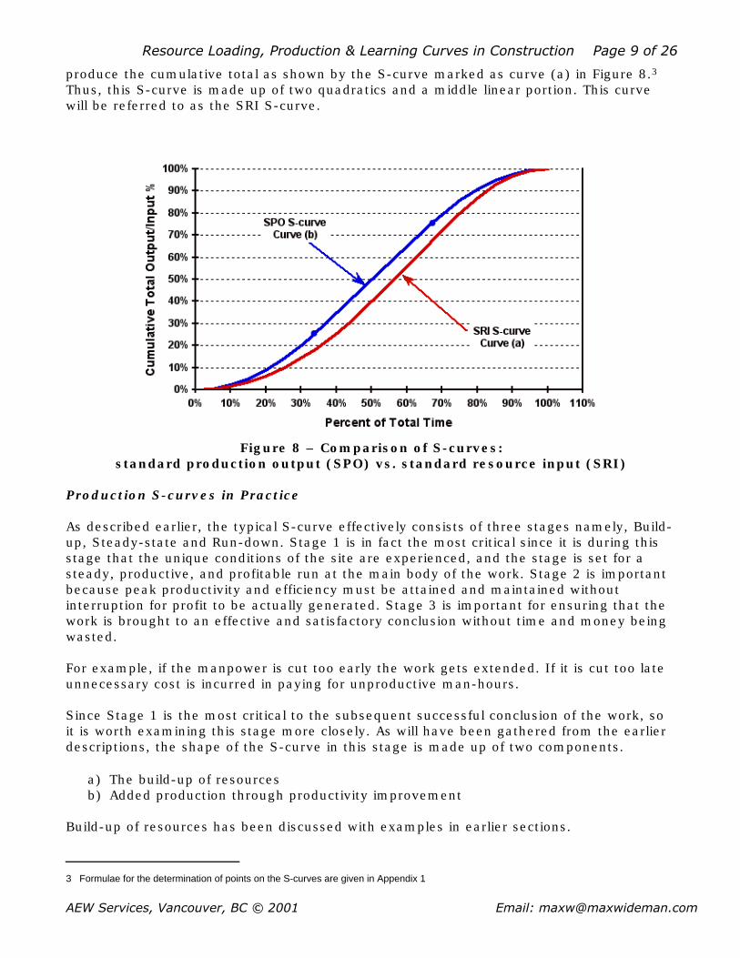
produce the cumulative total as shown by the S-curve marked as curve (a) in Figure 8.3Thus, this S-curve is made up of two quadratics and a middle linear portion. This curvewill be referred to as the SRI S-curve.

Figure 8 – Comparison of S-curves:standard production output (SPO) vs. standard resource input (SRI)

Production S-curves in Practice

As described earlier, the typical S-curve effectively consists of three stages namely, Build-up, Steady-state and Run-down. Stage 1 is in fact the most critical since it is during thisstage that the unique conditions of the site are experienced, and the stage is set for asteady, productive, and profitable run at the main body of the work. Stage 2 is importantbecause peak productivity and efficiency must be attained and maintained withoutinterruption for profit to be actually generated. Stage 3 is important for ensuring that thework is brought to an effective and satisfactory conclusion without time and money beingwasted.

For example, if the manpower is cut too early the work gets extended. If it is cut too lateunnecessary cost is incurred in paying for unproductive man-hours.

Since Stage 1 is the most critical to the subsequent successful conclusion of the work, soit is worth examining this stage more closely. As will have been gathered from the earlierdescriptions, the shape of the S-curve in this stage is made up of two components.

a) The build-up of resourcesb) Added production through productivity improvement

Build-up of resources has been discussed with examples in earlier sections.

3 Formulae for the determination of points on the S-curves are given in Appendix 1



Added production through productivity improvement implies that the rate of outputachieved will exceed that which might be inferred simply from examining the resourceloading. On a well-run project this is a key management expectation, which will bereflected in the shape and timing of the progress S-curve for the job. Indeed, this leads toa second simple empirical relationship.

Empirical Relation #2

A First Approximation to a Project Progress curve4

A first approximation to project progress or output is suggested by the following empiricalrelationship.§ 25% of total progress is achieved in the first third of the total time,§ Another 50% in the next third, and§ The remaining 25% in the last third.

This, a curve representing an accelerating rate of progress will be exhibited in the first25% of the time, while a similar but opposite curve will occur in the last third.

Like the SRI S-curve, this curve is also made up of two quadratics and a linear section inthe middle. For convenience it will be referred to as a "Standard Production Output" (SPO)S-curve. Note that if this profile is being used for planning or forecasting, the 100% TotalTime base will correspond to the realistically planned duration. If, however, the profile isbeing used for post completion analysis, the Actual Total Time may be substituted. Theunits of progress may be expressed in units appropriate to the work, such as excavationvolumes, numbers of piles, or value of work produced as shown in Figure 4.

The SPO S-curves is shown plotted as curve (b) in Figure 8. The differences between thetwo curves is essentially developed during Stage 1 of the S-curves, i.e. the first third ofthe Total Time. The shapes of the two curves are largely driven by the addition ofresources. However, if the difference is attributed to improvement through learning, it canbe shown that this difference is equivalent to a Learning Curve of 86% based on the LL-CA Model calculation discussed below. This is within the range of productivity-improvement-through-learning observed through independent measurements onconstruction sites.

Productivity Improvement Through Learning

The theory behind productivity improvement through learning is worth reviewing briefly,because there are somewhat different, though similar, approaches to the mathematicsinvolved. In addition, the theory can make a useful contribution in terms of:

§ Demonstrating the importance of consistent management direction andeffectiveness

§ Showing the benefits of establishing on a job the highest possible degree ofrepetition

§ Ensuring sufficient and continuous availability of work prior to commencement§ Underpinning work crew motivation and attitude§ Forecasting output, and hence time and cost to completion§ Estimating work which is comparable, but which may be significantly different in the

4 This empirical progress curve has been used on the job by the author for many years and has been offered to students in cost

management and cost control project management workshops.



amount to be accomplished.And conversely, in§ Demonstrating the adverse impacts of interference to the flow of work

Learning Curve vs. Experience Curve

The principle of the learning curve is given in Appendix 1. However, there is someconfusion in the construction industry regarding the use of this term. Because differentconstruction work typically takes place under unique conditions at a unique site, it isuseful to differentiate between productivity improvement due to “learning” and that due to“experience”.

As craft apprentices learn their trade, productivity increases. However, when skilled craftsperform a specific task on site and repeat it a number of times, there is a similarproductivity increase. The former increase is due to “learning the skill”, while the latter isdue to acquiring “experience of the particular site conditions” associated with the workactivity at the time.

This is an important distinction because it has significant implications if a site is not wellrun, or a job is subject to changes which interrupt the development of the learningpattern.

In construction, unfortunately, "learning curve" is typically used to refer to theproductivity improvement resulting from the site experience, that is, by crafts who arealready skilled at their trade. Consistent with this practice, this paper uses "learningcurve" to imply "experience" and therefore assumes that all crafts have already acquiredthe relevant skills for the work.

Original Theory

The phenomenon of "learning" was first expressed mathematically in 1936 by T. P.Wright. He observed in the aircraft industry that certain costs per unit tend to decrease ina predictable pattern as the workers and their supervisors become more familiar with thework. These decreasing costs are a function of a learning process in which fewer andfewer man-hours are required to produce a unit of work as more and more units areproduced. The key elements of the theory may be summarized as follows (Adrian 1987).

§ The repetition of any task leads to an improvement in productivity as a result of theexperienced gained.

§ This phenomenon is well established in the mass production industry as well as inthe construction industry under appropriate circumstances.

§ The application of the theory (in the construction industry) assumes that operativesstart with the necessary basic skills as well as the required support for the work tobe accomplished.

§ Productivity improvement then typically follows a constant ratio relationship whichis expressed as follows.

For every doubling of units, the cumulative average time per unit is reduced by aconstant ratio.

This relationship is illustrated in Table 1, showing examples of Cumulative Average Timeper Unit (Chellew 1974).



Number of Units in Cumulative Average Time per UnitSequence 90% Ratio 80% Ratio

1 100.0 100.02 90.0 80.04 81.0 64.08 72.9 51.2

16 65.6 40.932 59.1 32.8

Table 1: - Examples of Cumulative Average Time per Unit for Two Different Ratios

In Table 1, the time taken for the first unit is 100%. At a 90% ratio, the average timetaken for the first and second unit is 90%, i.e., the actual time taken for the second unit is80%. By the time the fourth unit is reached the average time taken for all four units is90%x90% = 81% and so on.

These values can be plotted as curves as shown in Figure 9. However, if the same data isplotted on log-log paper as shown in Figure 10, the result is a straight line which is moreuseful for manual analysis or mathematical illustration.

Figure 9 – Illustration of learning curves



Figure 10 – Learning curves plotted on log-log scale

Two Approaches

The above log-log relationship can be expressed mathematically as follows.

The cumulative average time (or cost) for each of 'n' units up to the nth unit, whenplotted against the number of units on log-log paper, produces a straight line.

This may be referred to as the “Log Linear - Cumulative Average Approach" (The LL-CAModel). This relationship is useful in forecasting or comparing similar operations but withsignificantly different numbers of units involved. It is also useful in analyzing largeamounts of data as, for example, the records of a large number of units produced from aprecasting yard. This is because the cumulative average curve has considerable power tosmooth out the unit data. It can also be deceptive because this power increases as thequantity increases (Thomas 1986). It is, therefore, less useful for examining theexpectations for individual units or the latest unit such as would be needed in trackingactual progress on a construction site.

This has led to a variation of the first relationship which states as follows.

The time (or cost) of the nth unit, when plotted against the number of units on log-logpaper, produces a straight line.

This may similarly be referred to as the "Log Linear - Unit Approach" (The LL-U Model)(Drewin 1982; DSMC 1989). The mathematics of both models are developed andcompared in Appendix 2. Table 2 shows calculations of the time to the nth unit and thetime of the nth unit over a range from one to fifty units for ratios ranging from 70% to95% as determined by each approach. The Cumulative Average figures are shown onwhite background, while the corresponding Cumulative Unit figures are shaded. As mightbe expected, the results of the two approaches are similar but not identical. The



differences in results obtained from the two approaches vary from about 7% for arepetition of only five units at a 95% productivity ratio to over 100% for 50 units at aratio of 70%.

Lp = r 0.950 0.900 0.850s=logr/log2 -0.074 -0.152 -0.234

Cum-Av Cum-Unit Cum-Av Cum-Unit Cum-Av Cum-Unitn Tn/U1 Un/U1 Tn/U1 U'n/U1 Tn/U1 Un/U1 Tn/U1 U'n/U1 Tn/U1 Un/U

1Tn/U1 U'n/U1

1 1.0 1.000 1.0 1.000 1.0 1.000 1.0 1.000 1.0 1.000 1.0 1.0005 4.4 0.829 4.7 0.888 3.9 0.675 4.4 0.783 3.4 0.538 4.2 0.686

10 8.4 0.784 9.0 0.843 7.0 0.602 8.1 0.705 5.8 0.452 7.3 0.58315 12.3 0.760 13.2 0.818 9.9 0.565 11.5 0.663 7.9 0.409 10.1 0.53020 16.0 0.743 17.2 0.801 12.7 0.540 14.8 0.634 9.9 0.382 12.6 0.49525 19.7 0.731 21.2 0.788 15.3 0.521 17.9 0.613 11.8 0.362 15.0 0.47030 23.3 0.721 25.1 0.777 17.9 0.507 20.9 0.596 13.5 0.346 17.3 0.45035 26.9 0.713 29.0 0.769 20.4 0.495 23.9 0.583 15.2 0.334 19.6 0.43440 30.4 0.705 32.8 0.761 22.8 0.485 26.7 0.571 16.8 0.323 21.7 0.42145 34.0 0.699 36.6 0.755 25.2 0.476 29.6 0.561 18.4 0.314 23.8 0.41050 37.4 0.694 40.3 0.749 27.6 0.469 32.4 0.552 20.0 0.307 25.8 0.400

Lp = r 0.800 0.750 0.700s=logr/log2 -0.322 -0.415 -0.515

Cum-Av Cum-Unit Cum-Av Cum-Unit Cum-Av Cum-Unitn Tn/U1 Un/U1 Tn/U1 U'n/U1 Tn/U1 Un/U1 Tn/U1 U'n/U1 Tn/U1 Un/U

1Tn/U1 U'n/U1

1 1.0 1.000 1.0 1.000 1.0 1.000 1.0 1.000 1.0 1.000 1.0 1.0005 3.0 0.418 3.9 0.596 2.6 0.314 3.7 0.513 2.2 0.224 3.4 0.437

10 4.8 0.329 6.6 0.477 3.8 0.230 5.9 0.385 3.1 0.152 5.2 0.30615 6.3 0.287 8.8 0.418 4.9 0.193 7.6 0.325 3.7 0.123 6.6 0.24820 7.6 0.261 10.8 0.381 5.8 0.171 9.2 0.288 4.3 0.105 7.8 0.21425 8.9 0.242 12.6 0.355 6.6 0.155 10.5 0.263 4.8 0.094 8.8 0.19130 10.0 0.228 14.3 0.335 7.3 0.144 11.8 0.244 5.2 0.085 9.7 0.17435 11.1 0.217 16.0 0.318 8.0 0.135 13.0 0.229 5.6 0.078 10.5 0.16040 12.2 0.208 17.5 0.305 8.7 0.127 14.1 0.216 6.0 0.073 11.3 0.15045 13.2 0.200 19.0 0.294 9.3 0.121 15.1 0.206 6.3 0.069 12.0 0.14150 14.2 0.193 20.5 0.284 9.9 0.116 16.1 0.197 6.7 0.065 12.7 0.134

= Cum-Av Approach = Cum-Unit Approach

Table 2 - Comparison of Cum. Av. and Cum. Unit Productivity from 70% to 90%

In practice, one would select one approach or the other depending on the objective, anduse the corresponding set of ratios. It does mean, however, that

When comparing the learning ratios on different jobs or of different crews on similarwork, the method of calculation must be the same and it must be specified.

Illustration of Learning Curve Application

For purposes of illustration, consider the following hypothetical case. The construction offloors on a 25 storey concrete high-rise building are being tracked. From the second floorup, all floors are virtually the same, so that the second floor is the first of a uniform seriesof 24. The roof and mechanical penthouse are not included in the observations.



Construction data is collected as follows.5

Time sheets are carefully marked up with job allocations, and hours are abstracted forforming and pouring concrete on each standard floor. The man-hours for the first in theseries is noted as 1175 man-hours. The second, third and fourth in the series take 855,905, and 735 respectively. This data is plotted on log-log paper using the LL-U Model asshown by line (a) in Figure 11. At this stage the data suggests a line whose slope is -.152(approx. 90% learning ratio) and that future floors would be expected to take the timesshown in Column 1b of Table 3.

Col 1a Col 1b Col 2a Col 2b Col 3

Floor# Observed Projected Observed Projected Final

4 floors 90%learning

6 floors 85%learning

All floors

1 1175 1175 1175

2 880 880 880

3 940 940 940

4 820 820 820

5 822 700 700

6 800 690 690

7 781 698 620

8 765 676 700

9 752 658 695

10 740 642 720

11 729 628 650

12 720 615 620

13 711 604 680

14 703 593 670

15 696 584 710

16 689 575 660

17 683 567 640

18 677 559 670

19 671 552 750

20 666 546 710

21 661 540 850

22 656 534 790

23 652 528 935

24 648 523 1060

Projected Totals:- 18036 15825

Final Total:- 18,335

Table 3 – High-rise repetitive construction: hypothetical case

However, suppose actual records for the next two floors, five and six, produce results of700 and 690 respectively. The addition of the latest data suggests a new line whose slopeis -.234 (approx. 85%) as shown by line (b) in Figure 11, and the new times taken tocomplete are as shown in Table 3, Column 2b. The new result shows a reduction in totalhours of approximately 2200 hours (12%, or the equivalent of some four extra floors).

5 The variation of “actuals” selected for the illustration are within the authors experience.



Figure 11 – High-rise repetitive construction:four floors projected (green), and six floors projected (turquoise)

Typically, practical reality follows neither of the two models. When record keeping iscontinued until all floors are completed, the results could be as shown in Table 3, Column3. These results are shown plotted in Figure 12.

Figure 12 – High-rise repetitive construction:cumulative unit projections and observed (LL-U model)



Many projects experience a decrease in productivity at the end of a run of work, (Barrie,Paulson 1978) and in the example the "tail end" departs significantly from either of thetwo earlier projections. The total man-hours shown in Table 3, Column 3 is 15% higherthan the second projected total in column 2b.

The same data, plotted according to the LL-CA Model, are shown in Figure 13. It will beseen that this model substantially conceals the significant changes in trends associatedwith the "tail end" effect. Thus, the LL-U Model, although not consistent with the originaltheory, is a more useful tool in many practical applications and for project managementobservation and control.

Figure 13 – High-rise repetitive construction:cumulative average projections and observed (LL-CA model)

When the figures shown in Table 3, Column 3 are plotted at normal scales, they display ashape sometimes referred to as the "Bath Tub" effect as shown in Figure 14. In fact, thisis simply a reflection of some of the considerations associated with each of the threestages of the S-curve discussed in an earlier section.

This suggests that the application of "Learning Curve Theory" on a construction siteshould be limited to the first 25% or so of the total production under consideration, whichis to say approximately 30-35% of the allotted time. In the high-rise constructionexample, the target for reaching optimum performance must be the 6th or 7th floor.

Issues Regarding Total Time and Stage 1 Time

A reasonable question to ask is how can the planner be assured of choosing the rightoverall time (i.e., equivalent to 100%) and why should the learning always take 30-35%of that value? Should it not be possible to contemplate a 36-storey high-rise, rather than24, and still achieve the Stage 2 efficiency of the 24 storey high-rise in the first six floors?



Figure 14 – High-rise repetitive construction:showing the "bath tub" effect

The practical reality is that if the building is that much larger in all likelihood the wholescale of the project operation is correspondingly larger and will be planned and organizedaccordingly. This includes increased use of temporary materials, plant, equipment and siteorganization all optimized to suit the larger project.

The planned time must also be realistic and achievable, especially if it is beingcompressed. Having chosen this time, it is essential that all the supporting logistics of thesite, including management, supervision, equipment, supplies etc., are all present tosupport this choice. Failing this, it is the author’s observation that the job then "takes on awill of its own" wherein it charts its own progress record. Thus, it is the organizationalculture associated with the site that ultimately determines the final outcome.

As one example of what can go wrong, Figure 15 compares actual production of rockexcavation with planned production on a less than well managed site preparationcontract.6 Partly due to changes, final quantities were significantly higher than originallyanticipated, the planned peak level of production was never reached, and Stage 1 of theS-curve took more time. Not surprisingly in this case, the whole contract took a lot longerto complete — and ended in litigation.

Conclusions

A review of resource input and production output on construction work shows threeseparate stages in any activity. This is true whether viewed at the task, trade, subcontractor whole project level. These stages constitute "build-up", "steady-state" and "run-down".Each stage has distinctive features.

6 From the author’s personal records of an actual contract.



Figure 15 – Comparison of actual vs. planned production of bulk rock excavation.Percent cumulative total is based on original estimate of 133 000 m3 (174,000

cubic yards)

If data over these three stages are viewed as a histogram of period resources input overthe duration of the work, a first approximation empirical profile can be articulated. That is:40% of resource input occurs in the first 50% of the time, a further 40% input in the next25% of the time and the remaining 20% in the last 25% of the time. This profiledetermines that peak loading will be 160% of the overall average.

If the same data is plotted as a running total on a percentage of total scale on both axes,the result is a typical S-curve. On a well-run project actual timing of this peak loading,i.e., Stage 2, appears to vary by only 10-15%.

As can be expected, production output follows a similar profile. However, if input andoutput S-curves are plotted to the same scales, the output S-curve will precede the inputS-curve to the extent that productivity improvement is achieved. For the whole of thiswork to be optimized, it appears that productivity improvement must essentially becompleted in Stage 1.

An empirical output or progress S-curve is suggested. This takes the form of one quarterof the progress in the first third of the time, another half in the next third and the finalquarter in the final third of the time. A realistic productivity improvement ratio of 86% inStage 1 would account for the difference between the two empirical S-curves of outputand input.

Obviously, the best source of information for planning and estimating is derived fromexperience of very similar previous work. In the absence of specific experience, however,these empirical relations can be used as a first approximation, particularly for early



planning.

Many construction projects offer various opportunities for repetitive work, though the totalnumber of repetitions may be small compared to manufacturing processes. However,when carefully managed and tracked, such work provides distinct opportunities forproductivity improvement. To optimize productivity gain, management energy must befocused on the first 25% of the series. The target must be to hit peak production withinone-third of the planned total time.

Two approaches to productivity improvement calculations are described. The first focuseson the Cumulative Average Time for 'n' units. However, the second, a modification of thefirst but focusing on the time taken for the nth unit, is more useful in most constructionapplications. In any case, it is suggested that the learning curve theory should not becarried further into the work than the first 25-30%.

Application of S-curve theory to construction work includes comparative estimating,forecasting, and quantifying the effects of delays upon performance. In these, the naturalloss of productivity in the final 25% of the work should also not be over looked.

References

Adrian, J. J. 1987. Construction Productivity Improvement. Elsevier Science PublishingCo., Inc., New York. p 154.

Allen, W. 1979. Developing the Project Plan. Notes prepared for Engineering Institute ofCanada Annual Congress Workshop. Toronto. pp 3-9.

Barrie, D. S. and Paulson, Jr. B. C. 1978. Professional Construction Management.McGraw-Hill, New York. p 224.

Chellew, J. H., 1974. The use of the learning curve. Proceedings PMISeminar/Symposium, Drexel Hill, Pennsylvania. p 163.

Christian, J., and Kallouris, G. 1991. An expert system for predicting the cost - timeprofiles of building activities. Canadian Journal of Civil Engineering, Vol. 18, 1991,Ottawa, Ontario. Fig. 3, p 814.

Defense Systems Management College, 1989. Applying Learning Curve Theory to ActualData. PMI Seminar/Symposium Education Workshop, Drexel Hill, Pennsylvania. p 1.

Drewin, F. J. 1982. Construction Productivity - Measurement and Improvement throughWork Study. Elsevier Science Publishing Co., Inc., New York. p 102.

Kerzner, H. 1989. Project Management: A Systems Approach to Planning, Scheduling, andControlling. Van Nostrand Reinhold, New York. pp 804-809.

Meredith, J. R. and Mantel, Jr. S. J. 1985. Project management - A Managerial Approach.John Wiley & Sons, New York. p 328.

National Electrical Contractors Association (NECA), 1983. Rate of Manpower Consumptionin Electrical Construction. Bethesda, Maryland. p 10.



Thomas H. R., Mathews C. T. and Ward J. G. 1986. Learning Curve Models of ConstructionProductivity. Journal of Construction Engineering and Management, ASCE, New York. p250.

Appendix 1

Definitions and Formulae adopted in this paper

Production (Rate)The rate at which units are produced over a given period of time, independent of thenumber of man-hours consumed.

ProductivityIn its broadest form, productivity may be described as a measure of how well theresources in a firm are brought together and used to accomplish a set of results.7 In itssimplest form, it may be expressed as the ratio of output to input or the actual rate ofoutput or production per unit of time worked.8 These represent measures of productionefficiency. When measurements are taken over a given period of time, the periodproductive efficiency is the number of units produced in that time period divided by thenumber of man-hours to do so.

S-curveWhen the cumulative total of on-going work on a construction job is plotted against time,the resulting curve typically follows the shape of the letter "S". It is more generallyreferred to as a Progress Curve.

Learning or Experience CurvesStudies have shown that the change in cost associated with a change in productivity has,in many situations, a characteristic curve that can be estimated with reasonable accuracy.This is called the “learning curve” or “experience curve”.9

The underlying phenomenon is that skill and productivity in performing tasks improve withexperience and practice and there are a number of different ways of plotting thisrelationship that facilitate mathematical analysis. Two models of Learning Curves aregiven in Appendix 2, Learning Curve Mathematics.

Well-runA well-run construction job implies that adequate and realistic planning has taken placeand a positive cultural environment has been established for the performance of the workon site. It also means that supporting logistics, including delivery of materials andequipment, have been properly assessed and will be provided when needed to enableoptimized crew sizes to maximize their production at least cost at each point in time. Itfollows that the resulting project should be perceived as successful in terms of meetingrequirements and being completed within credible time and cost parameters. For anowner this would mean that the resulting facility has satisfied the stipulated needs, withinreasonable time and budget. For a contractor, it would mean satisfying the owner at aprofit.

7 Cleland, D. I. 1990. Project Management Strategic Design and Implementation. TAB Books Inc. Blue Ridge Summit, Pennsylvania. 344.

8 Cleland, D. I. and Kerzner H. 1985. A Project Management dictionary of Terms. Van Nostrand Reinhold C. New York. 193.

9 Anthony, R. N. and Reece, J. S. 1975. Management Accounting: Text and Cases. Richard D. Irwin, Inc., Homewood, Illinois. 540.



In contrast, actual progress on a not-so-well-run job will depart from the plan or proceedas "a voyage of discovery". The records will likely reflect wasted manpower beforesufficient work is available or after it is substantially completed, lower productivity, highermanpower turnover, additional learning costs, added supervision, labour and non-labour-related job expenses and overhead, added material storage, handling and wastage, andextended completion.

Standard Resource Input curve (SRI S-curve)

Points on the SRI S-curve may be determined as follows:

In Stage 1: If t1 is a time between 0 and 50% then the cumulative total production isp = 0.5 t12 x 1.6/0.5

= 1.6 x t12

In Stage 2: If t2 is a time between 50% and 75%, then the cumulative total production is p = p50 + 1.6 (t2 - t50)or

p = 0.40 + 1.6 (t2 - 0.50) = 1.6 t2 - 0.40

In Stage 3: If t3 is a time between 75% and 100% then the cumulative total production is p = p75 + 0.8 (t100 - t75) - 0.8 (t100 - t3)2/ (t100 - t75)or p = 0.8 + 0.8 (1 - 0.75) - 0.8 (1 - t3)2/ (1 - 0.75) = 1 - 3.2 (1 - t3)2

Standard Production Output curve (SPO S-curve)

Points on the SPO S-curve may be determined as follows:

In Stage 1: If t1 is a time between 0 and 33.3% then the cumulative total production isp = 0.5 t12 x 1.5/0.333

= 2.25 t12

In Stage 2: If t2 is a time between 33.3% and 66.7%, then the cumulative totalproduction is

p = p33 + 1.5 (t2 - t33)or p = 0.25 + 1.5 (t2 - 0.333) = 1.5 t2 - 0.25

In Stage 3: If t3 is a time between 66.7% and 100% then the cumulative total productionis

p = p67 + 0.75 (t100 - t67) - 0.75 (t100 - t3)2/ (t100 - t67)



orp = 0.75 + 0.75 (1 - 0.667) - 0.75 (1 - t3)2/ (1 - 0.667) = 1 - 2.25 (1 - t3)2

Appendix 2

Learning Curve Mathematics

Learning Curve Mathematics is based on the observation that when a particular task orsequence of work is repeated without interruption certain costs per unit tend to decreasein a predictable pattern. This is attributed to the experienced gained as the workers andtheir supervisors become more familiar with the work being repeated. There are,however, two approaches or mathematical models for purposes of practical application.

Model A: Log Linear - Cumulative Average (LL-CA)

This model was first stated mathematically in 1936 by T. P. Wright who observed thatproductivity improvement typically follows a constant ratio relationship in the form

For every doubling of units, the cumulative average time per unit is reduced by aconstant ratio.

When plotted to log-log scale, the result is a straight line. Expressed more fully

The cumulative average time (or cost) for each of 'n' units up to the nth unit, whenplotted against the number of units on log-log paper, produces a straight line.

This is referred to as the Log Linear - Cumulative Average (LL-CA) Model.

Suppose the time for the first unit is taken as 100% and the ratio 'r' is 80%. then theaverage time for the first and second units is 80%. That is the second unit took 60% ofthe time of the first unit. By the time the fourth unit is reached, the average time takenfor all four units is 64% and so on.

Consider Figure (a) and the following relationships.

Symbols

Let Cn = y ordinate = Cumulative Average Time over 'n' units(CATn)

n = x ordinate = number of unitsN = n.th unit

U1 = Time to produce first unit (constant) = T1Un = Time to produce n.th unit

s = Slope of CAT line on log-log plotr = the constant ratio (by definition), otherwise known as the Learning

Curve Ratio; Learning Rate; Decremental Rate of Experience; Learning percent; PercentLearning etc. Usually expressed as 80%, 90% etc, and

s', r', = corresponding symbols for Model B



slope measured in non-log units e.g. 80%, 90% etcor s = negative slope "as plotted"

log n

=

nU 1

Cn

Figure A1: Typical learning curve plotted on a Log-Log scale

From Figure A1

By definition



Model B: Log Linear - Unit (LL-U)

Model A is useful in forecasting or comparing similar operations but with significantlydifferent numbers of units involved. It is less useful for examining results for individualunits as in tracking progress on a construction site. This has led to a variation which isexpressed as follows.

The time (or cost) of the nth unit, when plotted against the number of units on log-logpaper, produces a straight line.

This is referred to as the Log Linear - Unit (LL-U ) Model.

Again, assume that the time for the first unit is taken as 100% and the ratio 'r' is 80%.In this model, the reduction of time between the first and second unit will be 20%.Between the 2nd and 4th units it will be a further 20% and so on. That is to say, thefourth unit will take 64% of the time of the first unit. This is very different from Model Ain which the fourth unit must take about 48% of the first unit.

In Figure (a) the 'y' ordinate is now 'time per unit' (rather than Cumulative Average Timeper Unit). Using the symbols previously listed, the new relationship is expressed by

By definition

and

Integrating

or

and



Plotting Stage 1 of the Standard Progress Output (SPO) S-curve

In this case Model A is easier to use and the difference from Model B is minimal. Bydefinition of the SPO S-curve, the learning curve must "force fit" to the start of Stage 2,which is one quarter of the units at one third of the time and at the slope of Stage 2which, between points N and N+1, is two thirds.

Then from equation (3) above

or

In the special case where 100% of the units are being plotted against 100% of the time,the learning curve ratio can be calculated by trial and error to 71% or .

Thus

or

This curve is shown plotted as Stage 1 in figure 8.

Applying Resource Loading, Production & Learning Curves to ...

Documents

Transcript of Applying Resource Loading, Production & Learning Curves to ...