Applying Divide and Conquer Search

Algorithm in Traveling Salesman Problem

ESE 499 Senior Design Project

Heinz Schaettler (Supervisor) Washington University in St. Louis Electrical &Systems Engineering Associate Professor hms@wustl.edu (314) 935-6019 Campus Box 1127 One Brookings Drive St. Louis, MO 63130

Kevin Teng Systems Science Engineering Undergraduate Student kst1@go.wustl.edu (919)270-5435 6122 Waterman Blvd. St. Louis, MO 63112

Abstract

The Traveling Salesman Problem is a classical operations research problem that deals

with optimization, scheduling, and planning. The objective of this senior design project is to

implement a divide and conquer algorithm to code a more efficient search algorithm than

conventional exhaustive methods. Using Matlab, the Traveling Salesman Problem was perceived

as an incidence matrix and divided into smaller sub-matrices. The divide and conquer method

algorithm successfully processed the graph faster than exhaustive approaches. However, an

important note to make is that there is a trade-off for the faster data processing. Though far

slower, the exhaustive method produces all possible paths and possibilities, whereas the divide

and conquer method neglects many paths. This divide and conquer method can be incorporated

into larger graph problems to expedite search time and search for a relatively viable and

efficient solutions.

Introduction

The Traveling Salesman Problem (TSP) is a classical optimization problem often studied

in operations research and theoretical computer science. The general idea of the problem is

that a salesman is assigned to traveling

through a set of n cities, but can only visit

each city once and cities have specific

paths connecting to another city

(Schättler, 88-100). Given these

restrictions, the salesman’s goal is to find

the shortest, optimal path. Further complications can be added to the problem such as a path

cost or queue time at a city. For the purpose of this project, the graph is converted to a

Hamiltonian graph. The paths have no weight and the paths are undirected (Hamiltonian Path).

Essentially a Hamiltonian graph is a simplified version of TSP graph without cost or direction. To

clarify future references, cycles and graph henceforth mentioned will be Hamiltonian.

TSP and Hamiltonian cycle represents a general, broader class of combinatorial

optimization problems called NP-complete. Therefore a specific algorithm applied to the TSP

will also be applicable to all NP-complete problems (Hoffman and Padberg). The motivation of

study the TSP is its applicability in real-world use. Scheduling, city design, genome sequecing,

and computer algorithms are some of the many fields that TSP contributes to (TSP Applications).

Methods

In order to easily manipuate and configure parameter of TSP, we converted a TSP graph

into an incidence matrix. The idea behind the conversion is to have a more numerical

representation of the problem for easy management and for a way to actually code the

problem in Matlab. A incidence matrix, pertaining to a unique graph, defines each row as a

node (city). The sequential columns represent the possible connections to the row node by

using 0 and 1. 0 are defined as having no connection between a specific nodes and 1 confirms a

path between the nodes. For simplification of the project, cost and direction between nodes

are omitted.

[ ]

Incidence matrix Graph

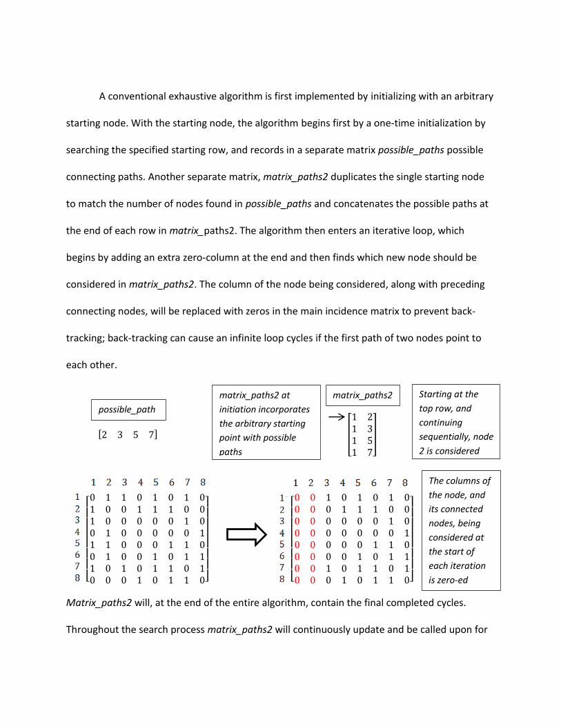
A conventional exhaustive algorithm is first implemented by initializing with an arbitrary

starting node. With the starting node, the algorithm begins first by a one-time initialization by

searching the specified starting row, and records in a separate matrix possible_paths possible

connecting paths. Another separate matrix, matrix_paths2 duplicates the single starting node

to match the number of nodes found in possible_paths and concatenates the possible paths at

the end of each row in matrix_paths2. The algorithm then enters an iterative loop, which

begins by adding an extra zero-column at the end and then finds which new node should be

considered in matrix_paths2. The column of the node being considered, along with preceding

connecting nodes, will be replaced with zeros in the main incidence matrix to prevent back-

tracking; back-tracking can cause an infinite loop cycles if the first path of two nodes point to

each other.

[ ] [

]

[ ]

[ ]

Matrix_paths2 will, at the end of the entire algorithm, contain the final completed cycles.

Throughout the search process matrix_paths2 will continuously update and be called upon for

The columns of

the node, and

its connected

nodes, being

considered at

the start of

each iteration

is zero-ed

matrix_paths2 matrix_paths2 at

initiation incorporates

the arbitrary starting

point with possible

paths

Starting at the

top row, and

continuing

sequentially, node

2 is considered

possible_path

ss

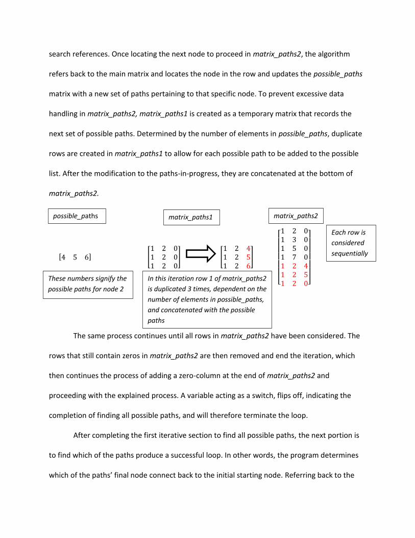
search references. Once locating the next node to proceed in matrix_paths2, the algorithm

refers back to the main matrix and locates the node in the row and updates the possible_paths

matrix with a new set of paths pertaining to that specific node. To prevent excessive data

handling in matrix_paths2, matrix_paths1 is created as a temporary matrix that records the

next set of possible paths. Determined by the number of elements in possible_paths, duplicate

rows are created in matrix_paths1 to allow for each possible path to be added to the possible

list. After the modification to the paths-in-progress, they are concatenated at the bottom of

matrix_paths2.

[ ] [

] [

]

[ ]

The same process continues until all rows in matrix_paths2 have been considered. The

rows that still contain zeros in matrix_paths2 are then removed and end the iteration, which

then continues the process of adding a zero-column at the end of matrix_paths2 and

proceeding with the explained process. A variable acting as a switch, flips off, indicating the

completion of finding all possible paths, and will therefore terminate the loop.

After completing the first iterative section to find all possible paths, the next portion is

to find which of the paths produce a successful loop. In other words, the program determines

which of the paths’ final node connect back to the initial starting node. Referring back to the

matrix_paths2 possible_paths

These numbers signify the

possible paths for node 2

matrix_paths1

In this iteration row 1 of matrix_paths2

is duplicated 3 times, dependent on the

number of elements in possible_paths,

and concatenated with the possible

paths

Each row is

considered

sequentially

initial main incidence matrix, without column editing, the non-zero elements of the starting

node column are determined. An additional zero-column is added to the matrix_paths2 to

leave space for editing and concatenation. The non-zero elements found in the starting node

column of the incidence matrix refer to nodes that have connections back to the starting node.

So cycling through the ending elements of each matrix_paths2 row, the paths that can

complete a Hamiltonian cycle are found. If the ending element of a row in matrix_paths2 does

not match one of the cycle nodes, the ending elements of that path will remain zero.

Conversely, if a matching node is found during the comparison, the starting node will be added

as a final element to that specific row in matrix_paths2. Completing each row comparison, the

paths that contain a zero at the end are deleted.

[ ]

[ ]

Another problem still exists after the completion of finding the cycles. Given the

exhaustive search algorithm properties, duplicate paths will form. So the next part of the

algorithm deletes the duplicate cycles. A separate delete matrix is created to keep track of

which rows should be deleted. Starting at the top of matrix_paths2, the cycle is reversed and

compared with each following cycle. The reason for reversing the cycle and then comparing is

because the duplicate cycles will be in reversed form of each other since the exhaustive method

will find both forward and reverse cycles. If two rows compared are identical, the row is

incidence matrix matrix_paths2

Connecting nodes are

found in the first column

in the incidence matrix

and compared to the

final elements of

matrix_paths2 and

added if they match

recorded and deleted immediately and jumps to the next row to be considered. Following this

process, matrix_paths2 will finally be left with all complete cycles for the specific TSP.

For the divide and conquer algorithm, given a TSP incidence matrix, the algorithm will

first divide the matrix into two separate sub-matrices. Splitting the matrix into four quadrants,

the second and fourth quadrants are the main focuses. Treating the two quadrants as separate

matrices, they are processed through the previously mentioned exhaustive search algorithm,

but stopping before finding cycles within the smaller sub-matrices.

[ ]

After running through the sub-searches the algorithm will produce two separate

matrices, matrix_paths_1 and matrix_paths_21, that contain path-pieces. For matrix_paths_2 a

simple equaton of matrix_paths_2 + a/2 is applied, variable “a” being the size of the incidence

matrix. Since the index of the fourth quadrant sub-matrix will be shifted, the equation is applied

to recalibrate the nodes to their correct indices. The unique elements of the first and last

columns of both matrix_paths_1 and matrix_paths_2 are determined and stored in four

matrices: link1, link2, link3, link4. The four matrices serve as a reference to see which ends of

the path-pieces connect. Starting with link1, each connective node is identified from the

incidence matrix and paths are identified from quadrant one. The identified paths are then

compared with link3 and link4. If there is a path between matrix link1 and link3 or link1 and

1 These matrices have different names from the code for clarification

incidence matrix Given an incidence

matrix, the divide and

conquer algorithm splits

the original matrix into

four quadrants

The second and fourth

quadrant sub-matrices are the

focus and are passed through

the exhaustive search

algorithm

link4, the path-piece pertaining to the identified node in link1 is called and combined with the

path-piece from link3 or link4. Depending on which node link1 is connected to, the

matrix_paths_1 path-piece will have to be reverse to correctly form the path. The same

procedure is used with link2 to obtain all possible paths.

[ ] [

]

[ ]

After piecing together the paths-pieces into a complete path in a new matrix matrixpaths, the

same procedure as described in the exhaustive method is used to find cycles and eliminate

duplicate paths.

Data and Analysis

Several tests were applied to both exhaustive and divide and conquer methods to

obtain detailed results. Beginning with the exhaustive search, a simple script was coded to

observe and plot the amount of time the algorithm took, beginning with a 3 by 3 matrix. With

each successive iteration, the matrix would increase by one node. A single circular path was

incorporated into the graph to ensure that no errors would occur when running the script. The

results of 350 iterations are shown in Figure 1. As one can see, the amount of time for each

matrix_paths_1 matrix_paths_2

link1 link2 link4 link3

incidence matrix

paths are identified in

quadrant 1 using link1

and link2 to determine

which nodes to refer to

0 50 100 150 200 250 300 350 4000

0.02

0.04

0.06

0.08

0.1

0.12

0.14

0.16

0.18

0.2

Nodes

Run T

ime (

s)

Run Time in Relation to Graph Size

Figure 1. Results of running the algorithm with

a matrix increasing by one node each iteration

0 5 10 15 20 250

10

20

30

40

50

60

70

80

Paths

Run T

ime (

s)

Run Time in Relation to Graph Complication

Figure 2. Results of running the algorithm with a matrix

increasing complexity by one path each iteration

successive iteration increases. However, most notable are the initial and ending changes. At

around 3 to 50 nodes, the time increases in a linear fashion. After reaching past 100 nodes, the

increase in time became more and more similar to an exponential function. Given that every

computer runs differently and often fluctuates due to hardware, background processes, and

external factors, fluctuations are unavoidable.

The next test that was conducted was to

increase the complexity of a graph with

each iteration. A 8 by 8 matrix is designed

to be sparse with only a circular cycle

path running through the graph. With each

iteration a path is connected between two

nodes. The diagonal of the incidence matrix,

however, must remain zero at all times. If

any element on the diagonal should be 1, it

signifies that a node has a path connecting

to itself, which is fundamentally incorrect

and will create errors when running

through the algorithm. Figure 2 shows the

results of the test. As one can see, the time

taken to complete the search increases

much more dramatically. Initially, the

change in time is almost nothing, however after more than 15 extra paths have been

incorporated into the matrix, the time increase drastically. An odd relative drop at around 21

paths appears consistently each time the test script is executed. My only guess is that the extra

paths generated at 20 and 21 do not generate too many extra cycles, which therefore will not

consume as much time.

Figure 3 to Figure 7 are data plots of the exhaustive method when a specified graph with

a certain percentage of spareness is determined.

0 10 20 30 40 50 60 70 80 90 1004

5

6

7

8

9

10

11

12

13x 10

-4 Computation Time 30% Fill with Graph Size 8

nth loop (Iteration)

Tim

e (

s)

0 10 20 30 40 50 60 70 80 90 1005

6

7

8

9

10

11

12

13x 10

-4 Computation Time 30% Fill with Graph Size 10

nth loop (Iteration)

Tim

e (

s)

0 10 20 30 40 50 60 70 80 90 1000.6

0.8

1

1.2

1.4

1.6

1.8x 10

-3 Computation Time 30% Fill with Graph Size 12

nth loop (Iteration)

Tim

e (

s)

0 10 20 30 40 50 60 70 80 90 1000.8

1

1.2

1.4

1.6

1.8

2

2.2

2.4

2.6x 10

-3 Computation Time 30% Fill with Graph Size 15

nth loop (Iteration)

Tim

e (

s)

Figure 3. Graph size

8 with random paths

generated at 30% fill

Figure 4. Graph size

10 with random paths

generated at 30% fill

Figure 5. Graph size

12 with random paths

generated at 30% fill

Figure 6. Graph size

15 with random paths

generated at 30% fill

Figure 7. A compilation of the graphs of different

sizes with randomly generated paths all with 30% fill

0 10 20 30 40 50 60 70 80 90 1000.4

0.6

0.8

1

1.2

1.4

1.6

1.8

2

2.2

2.4x 10

-3Computation Time between Graphs of Different Size and 30% Fill

nth loop (Iteration)

Tim

e (

s)

The dotted line apparent in Figure 3 to Figure 6 is the average run time for the specific graph.

As one can observe, the fluctuations are always random with each successive script run.

However, a very apparent trend is that there will generally always be some run times that are

greatly above and below relative to the average run time. This is due to the fact that the

randomly generated paths sometimes will generate more complete cycles, which will increase

the processing time for that specific

iteration. As expect, with the

increase of graph size the average

run time will be slower.

Something worth noting is the

combination plot in Figure 7. As one

can see, most of the run time for

the smaller graphs will be below the

time of larger graphs. However, there

are still a significant number of iterations that come close or even exceed the run time of a

larger graph. The impact of a graph’s run time is more dependent on the complexity of the

graph. Size does indeed play a role in how slow the graph is processed, as seen from the

previous exhaustive experiments; however, the graph complexity will play a larger role in

determining the run time.

0 10 20 30 40 50 60 70 80 90 1002

2.5

3

3.5

4

4.5

5

5.5x 10

-4 Computation Time with 100 Runs

nth loop(Iteration)

Run T

ime (

s)

Figure 8. Divide and conquer processing

an 8 node graph over 100 iterations

0 10 20 30 40 50 60 70 80 90 1001.5

2

2.5

3

3.5

4

4.5

5x 10

-4 Computation Time with 100 Runs

Run Times (Loop)

Run T

ime (

s)

Figure 9. Divide and conquer processing

different sized graphs over 100 iterations

Figure 8 and Figure 9 are data obtained from testing the divide and conquer algorithm.

Figure 8 shows the run time over 100 iterations.

What is very noticeable is that there are almost

no iteration that have a run time close to the

average run time. Though there are some, the

occurrence is very low. Most of the iterations

have a run time significantly higher or lower than

the average run time.

Figure 9 shows a plot comparing the run

time of several graphs of different sizes. Similar to

the exhaustive method, the run times often vary

and sometimes run longer than graph sizes

that are larger. One very peculiar thing to note

is that the blue graph, with a graph size of 20

nodes, has a significantly higher run time than

the preceding 18 node graph. I speculate that

similar to the exhaustive search method, the

larger the graph size becomes, exponentially longer the run time will be. However, it must be

noted that the run time is still on the scale of 10-4 seconds whereas the exhaustive method

would already be in the 10-3 realm. The increase in time mathematically is still considerably

small, but in the graphical perspective, the average increase run time is quite distinguishable.

0 10 20 30 40 50 60 70 80 90 1001

2

3

4

5

6

7x 10

-3 Computation Time with 100 Runs

nth loop (Iterations)

Run T

ime (

s)

Figure 10. Comparison of run times between

exhaustive and divide and conquer methods

Given the same graph, both algorithms were applied with 100 iterations. Figure 10

shows the run time comparison between the two methods. The blue plot is the run time for the

divide and conquer method and the red

plot is the run time for the exhaustive

search method. The difference between

the two is quite large. Theoretically,

the divide and conquer should indeed

run at a faster speed, since as we

observed in the exhaustive algorithm

data, the larger the graph, the longer the time

it takes to compute in an exponential behavior.

And since the divide and conquer method does incorporate the exhaustive method, but with

smaller matrices, it should be considerably faster, and the difference should be apparent in

larger graph sizes. Again, it is noted that there are sometimes very large spikes in the graph, as

one can see in Figure 10, at around the 58th iteration. There is an enormous run time spike that

comes close or even surpasses the exhaustive method run time.

This random outlier was probably caused by a sudden hiccup in the computer’s

background process. But it is also possible that at a small enough graph size, the divide and

conquer method may run slower. Due to the fact that the divide and conquer will split the

original graph to two sub-matrices, the extra computation in dividing and comparing paths-

pieces can possibly increase run time and run slower than the exhaustive method for small

graphs. Figure 11 shows the comparison between the exhaustive and divide and conquer

0 50 100 150 200 250 300 3500

0.05

0.1

0.15

0.2

0.25

0.3

0.35

0.4

0.45

0.5Split and Exhaustive Comparison

Graph Size (Nodes)

Run T

ime (

s)

Figure 11. Comparison between exhaustive and

divide and conquer method with increasing graph

size per iteration

method when computing for a graph whose size increases by one node each iteration. The red

plot defines the exhaustive search algorithm and the blue line denotes the divide and conquer

method. The run time speed for the

exhaustive search is considerably slower

than that of the divide and conquer

method. Towards the largest graph size

tested, a 350 node graph, the exhaustive

search reaches almost 0.5 seconds to

complete whereas the divide and

conquer method reaches a value close to

0.1 seconds. The difference in run time is quite large with larger graph sizes. At the small graph

sizes, the two algorithms run quite well until about 50 nodes, when the speed differentiation

becomes more apparent. At the earlier stages, the divide and conquer can still possibly run

slower, as one can see at around 10 nodes the divide and conquer method had a considerably

slower run time. The outlying point can also be a product of the computer’s error; however, I

think it is a high possibility that in some certain graphs the divide and conquer can be slower

than the exhaustive method. Overall, only a small percentage of graphs will run more efficiently

by utilizing the exhaustive method.

To further investigate the behavior of the exhaustive and divide and conquer method, I

processed the logarithmic run time of the two systems. The graph would plot a linear behavior

if the algorithm is exponential. But shown in Figure 12, the behavior of the exhaustive search is

Figure 12. A quadratic plot fitting to the

exhaustive search algorithm

0 50 100 150 200 250 300 350-8

-7

-6

-5

-4

-3

-2

-1

0

Graph Size (Nodes)

Logarith

mic

Run T

ime

Exhaustive Logarithmic Analysis

y = - 3.7e-005*x2 + 0.028*x - 6.3

y = 1.9e-007*x3 - 0.00014*x2 + 0.043*x - 6.8

y = - 1.3e-009*x4 + 1.1e-006*x3 - 0.00035*x2 + 0.06*x - 7.1

data 2

quadratic

cubic

4th degree

Figure 13. Extra cubic and 4th degree

fitting plots to the exhaustive algorithm

0 50 100 150 200 250 300 350-8

-7

-6

-5

-4

-3

-2

-1

0

Graph Size (Nodes)Logarith

mic

Run T

ime

Exhaustive Logarithmic Analysis

y = - 3.7e-005*x2 + 0.028*x - 6.3

data 2

quadratic

a quadratic polynomial. As the script

runs, one can see the slow plateau

behavior of the graph. Converting the

logarithmic back to the original run

time, the curve would be escalating

upwards faster. Figure 12 also shows a

basic fitting of the logarithmic plot.

Using the built-in Matlab fitting tools, the basic

behavioral equation is in the form

of . Testing out higher

order plot fittings, though do

increase the accuracy, but not

significantly. It can probably be

concluded that the behavior

closely resembles a quadratic

function. Figure 13 shows other

basic fittings to the exhaustive method. The

divide and conquer has a similar behavior to

the exhaustive search, since both apply the same basic foundation. The divide and conquer

method just performs the task to a much more efficient degree.

Conclusion

The divide and conquer method indeed does have a much more efficient search pattern

compared to that of the exhaustive search. However, it must be noted that the divide and

conquer method does not find every single possible cycle. Contrary to the divide and conquer,

the exhaustive method can successfully list out all the paths, but at a high time consuming cost.

Though reliable in the sense that given a smaller problem, the solution can be quickly searched

and optimized. However, in many worldly problems, the graph size is often of large magnitude,

and requires a faster algorithm. Given the massive size of some optimization problems, it is

sometimes ideal to forgo optimal solutions and settle for a reasonable option calculated in a

faster method.

In this respect, the divide and conquer method is a viable approach in solving NP-

complete optimization problems, as it performs computational task faster than brute force

exhaustive methods. In a larger graph scenario, the divide and conquer will be able to calculate

a reasonable solution within a shorter period time and is more pragmatic compared to the

exhaustive method.

Future Motivations and Studies

TSP is a highly studied topic and its applications are very widespread. One major topic

that can utilize this TSP divide and conquer method is genome sequencing. The purpose of

genome sequencing is to determine the DNA sequence of an organism’s genome. The

applications of understanding the complete details and structure of a genome can lead to many

scientific development and studies involved in medicinal and evolutionary fields. However, the

major obstruction is the sheer length of genomes. The time to sequence a genome, is vastly

unreasonable and long.

To confront this issue, geneticists often break up and split long genome sequences into

smaller pieces. Translating each smaller portion, the geneticists mark each piece with a marker,

which denotes the likelihood of the specific piece following another. One can conceptualize this

as a TSP, where each genome piece represents a node and the likelihood that a piece follows

another acts as a path with a cost (TSP Applications). The divide and conquer search algorithm

can possible play a part in expediting genome sequencing with its efficient search properties,

especially since the divide and conquer method far exceeds the exhaustive search method in

larger exhaustive problems.

References

"Hamiltonian Path." Wikipedia, the Free Encyclopedia. 05 May 2005. Web. 05 Dec. 2011.

<http://en.wikipedia.org/wiki/Hamiltonian_path>.

Hoffman, Karla, and Manfred Padberg. "The Traveling Salesman Problem." Web. 05 Dec. 2011.

<http://iris.gmu.edu/~khoffman/papers/trav_salesman.html>.

Schättler, Heinz. “Operations Research.” Powerpoint presentation for Introduction to Systems

Science and Engineering, Washington University in St. Louis. Fall 2010

"TSP Applications." Traveling Salesman Problem. Jan. 2007. Web. 05 Dec. 2011.

<http://www.tsp.gatech.edu/apps/index.html>.

Appendices

A 1.

Matlab script for exhaustive search algorithm

%Given problem

%A = [0 1 0 1; 1 0 1 0; 0 1 0 1; 1 0 1 0]

%A = [0 1 1 1; 1 0 1 1; 1 1 0 1; 1 1 1 0]

% A = [0 1 1 0 1 0 1 0; 1 0 0 1 1 1 0 0; 1 0 0 0 0 0 1 0; 0 1 0 0 0 0 0 1; 1

1 0 0 0 1 1 0 ; 0 1 0 0 1 0 1 1 ; 1 0 1 0 1 1 0 1 ; 0 0 0 1 0 1 1 0];

function [matrix_paths2 run_time] = matrix_paths(A)

tic %starts the timing of the process

%Initializing variables

C = A; % matrix for modification

button = 0; %condition to stop looping

starting = 1;

matrix_paths1 = [];

matrix_paths2 = [];

%initializing phase to start off the operation

possible_paths = find(C(starting(1),:)); %find the possible continuing pathes

a = size(possible_paths,2); %checks to see initially how many paths are

possible

matrix_paths2 = zeros(a,1); %creates a column of zeros to start adding

matrix_paths2(:,1) = starting; %sets the first column to be the starting

point

matrix_paths2(:,2) = possible_paths'; %transposes possible paths and add it

onto the first point

%Actual cycling and looking for paths

while (button == 0)

k = size(matrix_paths2,2); %used to search the correct column

matrix_paths2(:,end+1) = 0; %creates a column of zeros to fix

concatenation issue

for i = 1:size(matrix_paths2,1)

starting = matrix_paths2(i,k); %changes which row we starting

searching for paths

C(:,matrix_paths2(i,1:k)) = 0; %modifies C for that specific path

possible_paths = find(C(starting,:)); %finds all possible connections

for that specific path

if(isempty(possible_paths)==0) %this confirms that there is a

available path. if not a zero is added at the end

%let that line be eliminated after the inner for loop

p = size(possible_paths,2); %sets the number path duplication

needed

else %if no available path is given, set the next path to be zero so

it can be deleted later on

p = 1;

possible_paths = 0;

end

for j = 1:p

matrix_paths1 = [matrix_paths1;matrix_paths2(i,:)]; %creates

additional paths, manual concatentation

end

matrix_paths1(:,end) = possible_paths'; %adds those paths to

matrix_paths1

matrix_paths2 = [matrix_paths2;matrix_paths1]; %concatenates those

new paths at the BOTTOM of matrix_paths2

matrix_paths1 = []; %resets matrix_paths1 for the next cycle

if(size(matrix_paths2,2) == size(A,2)) %checks to see the termination

condition

button = 1; %sets the button to 1 to temrinated the while loop

end

C = A; %resets matrix C for other paths

end

[x,y] = find(matrix_paths2 == 0); %finds all rows that have zeros

matrix_paths2(x',:) = []; %deletes those rows, as they are not needed

end

%Section checks for complete loops

[q,w] = find(A(:,matrix_paths2(1,1))); %figures out which pathes will have a

complete loop

[e,r] = size(matrix_paths2);

matrix_paths2(:,end+1) = 0; %adds an extra column of zeros so additional

paths can be added

for t = 1:e

if(find(q' == matrix_paths2(t,end-1)) > 0) %if the end element of a paths

exists in q, then it is

%a complete cycle

matrix_paths2(t,end) = matrix_paths2(t,1); %completes the loop if it

exists

else

matrix_paths2(t,end) = 0; %tags a zero if it isn't a complete loop

end

end

[x,y] = find(matrix_paths2 == 0); %finds all rows that have zeros

matrix_paths2(x',:) = []; %deletes those rows, as they are not needed

%This section deletes the repeats

delete = []; %keeps track on the row number to be deleted

counter = 1; %counter to increment the row

while(size(delete,2) <= size(matrix_paths2,1)/2) %termination factor is

decided by when the delete matrix size

%is less than equal to half the number of rows of matrix paths

o = size(matrix_paths2,1); %resets the for loop, since we are editing the

paths directly

for u = 1:o

if(fliplr(matrix_paths2(counter,:)) == matrix_paths2(u,:))%checks to

see if two rows are the same

delete(end+1) = u; %adds to the delete matrix

matrix_paths2(u,:) = []; %deletes the row if condition is met

break %once condition is met, jump out of the for loop

end

end

counter = counter + 1; %increases the counter

end

matrix_paths2;

toc; %ends the timing on the process

run_time = toc;

A 2.

Matlab base script for divide and conquer algorithm.

function [matrix_paths2] = matrix_split_graph(A)

%Initializing variables num_starting = find(sum(A,2) == 1); %finds the row that only have one path starting = []; %initializing the variable if (size(num_starting,1) > 2) %if any sub-matrix has more than three nodes

with more one path, we can conclude that %the sub matrix we arbitrated is in more than one piece error('Sub-matrix has broken subsections') elseif (isempty(num_starting) == 1) %if no node has a single path, choose

first node arbitrarily starting = 1; else starting = num_starting(1); %randomly choose one of the two (if two exist)

as a starting point end C = A; % matrix for modification button = 0; %condition to stop looping beginning = starting; matrix_paths1 = []; matrix_paths2 = [];

%initializing phase to start off the operation possible_paths = find(C(starting(1),:)); %find the possible continuing pathes a = size(possible_paths,2); %checks to see initially how many paths are

possible matrix_paths2 = zeros(a,1); %creates a column of zeros to start adding matrix_paths2(:,1) = starting; %sets the first column to be the starting

point matrix_paths2(:,2) = possible_paths'; %transposes possible paths and add it

onto the first point

%Actual cycling and looking for paths while (button == 0) k = size(matrix_paths2,2); %used to search the correct column matrix_paths2(:,end+1) = 0; %creates a column of zeros to fix

concatenation issue for i = 1:size(matrix_paths2,1) starting = matrix_paths2(i,k); %changes which row we starting

searching for paths C(:,matrix_paths2(i,1:k)) = 0; %modifies C for that specific path possible_paths = find(C(starting,:)); %finds all possible connections

for that specific path if(isempty(possible_paths)==0) %this confirms that there is a

available path. if not a zero is added at the end %let that line be eliminated after the inner for loop p = size(possible_paths,2); %sets the number path duplication

needed else %if no available path is given, set the next path to be zero so

it can be deleted later on

p = 1; possible_paths = 0; end for j = 1:p matrix_paths1 = [matrix_paths1;matrix_paths2(i,:)]; %creates

additional paths, manual concatentation end matrix_paths1(:,end) = possible_paths'; %adds those paths to

matrix_paths1 matrix_paths2 = [matrix_paths2;matrix_paths1]; %concatenates those

new paths at the BOTTOM of matrix_paths2 matrix_paths1 = []; %resets matrix_paths1 for the next cycle if(size(matrix_paths2,2) == size(A,2)) %checks to see the termination

condition button = 1; %sets the button to 1 to temrinated the while loop end C = A; %resets matrix C for other paths end [x,y] = find(matrix_paths2 == 0); %finds all rows that have zeros matrix_paths2(x',:) = []; %deletes those rows, as they are not needed end

%This section deletes the repeats matrix_paths2(:,1) = [] % deletes the first column delete = []; %keeps track on the row number to be deleted counter = 1; %counter to increment the row button2 = 0; %to keep track when to terminate the loop while(button2 == 0) %termination factor is decided by when the delete matrix

size %is less than equal to half the number of rows of matrix paths o = size(matrix_paths2,1); %resets the for loop, since we are editing the

paths directly for u = 1:o if(fliplr(matrix_paths2(counter,:)) == matrix_paths2(u,:))%checks to

see if two rows are the same delete(end+1) = u; %adds to the delete matrix matrix_paths2(u,:) = [] %deletes the row if condition is met break %once condition is met, jump out of the for loop end end o = size(matrix_paths2,1); counter = counter + 1; %increases the counter if(counter >= o) %if the counter is the same size or greater than o we

have reached the bottom of the matrix button2 = 1; %flips the switch to break out of the loop end end matrix_paths2 = fliplr(matrix_paths2); %flips the matrix left-right matrix_paths2(:,end+1) = beginning %adds the column back to the end matrix_paths2 = fliplr(matrix_paths2) %flips the matrix left-right again

A 3.

Second part of divide and conquer method that calls upon A 2 script.

clean runtime = [];

A = [0 1 1 0 1 0 1 0; 1 0 0 1 1 1 0 0; 1 0 0 0 0 0 1 0; 0 1 0 0 0 0 0 1; 1 1

0 0 0 1 1 0 ; 0 1 0 0 1 0 1 1 ; 1 0 1 0 1 1 0 1 ; 0 0 0 1 0 1 1 0]; a = size(A,1); %keeps a size to calibrate index [matrix_paths] = matrix_split_graph(A(1:4,1:4)); %runs first submatrix [matrix_paths2] = matrix_split_graph(A(5:8,5:8)); %runs second submatrix matrix_paths2 = matrix_paths2 + a/2; %modifies the index of second submatrix

to be consistent clc [x,y] = size(matrix_paths); %finds the unique elements in the first and last column of each submatrix link1 = transpose(unique(matrix_paths(:,1))); link2 = transpose(unique(matrix_paths(:,end))); link3 = transpose(unique(matrix_paths2(:,1))); link4 = transpose(unique(matrix_paths2(:,end)));

matrixpaths = []; counter = 1; %to index matrixpaths correctly %checks to see which nodes connect to the front of the first submatrix %using the front of the second submatrix for u = 1:101 tic for i = 1:size(link1,2) connection = find(A(link1(i),a/2+1:a)) + a/2; %finds all possible

connections for specific node link1_3 = ismember(link3, connection); %checks to find if such

element links to the front of the second submatrix link1_4 = ismember(link4, connection); %checks to find if such

element links to the end of the second submatrix if(nnz(link1_3 == 1)) %if there are nonzero elements in link1_3 [q,w] = find(matrix_paths(:,1) == link1(i)); %find the positions

of the rows [e,r] = find(matrix_paths2(:,1) == link3(find(link1_3))); %find

the positions of the rows for p = 1:size(e) for o = 1:size(q) matrixpaths(counter,:) =

[fliplr(matrix_paths(q(o),:)),matrix_paths2(e(p),:)]; %combines the two

matrices counter = counter + 1; %increment counter end end end %checks to see which nodes connect to the front of the first

submatrix %using the end of the second submatrix if(nnz(link1_4 == 1)) [q,w] = find(matrix_paths(:,1) == link1(i)); [e,r] = find(matrix_paths2(end,:) == link4(find(link1_4)));

for p = 1:size(e) for o = 1:size(q) matrixpaths(counter,:) =

[matrix_paths2(e(p),:),matrix_paths(q(o),:)]; counter = counter + 1; end end end end

%same procedure but connects to the end of the first submatrix for i = 1:size(link2,2) connection = find(A(link2(i),a/2+1:a)) + a/2; link2_3 = ismember(link3, connection); link2_4 = ismember(link4, connection); if(nnz(link2_3 == 1)) [q,w] = find(matrix_paths(:,end) == link2(i)); [e,r] = find(matrix_paths2(:,1) == link3(find(link2_3))); for p = 1:size(e) for o = 1:size(q) matrixpaths(counter,:) =

[matrix_paths(q(o),:),matrix_paths2(e(p),:)]; counter = counter + 1; end end end if(nnz(link2_4 == 1)) [q,w] = find(matrix_paths(:,end) == link2(i)); [e,r] = find(matrix_paths2(:,end) == link4(find(link2_4))); for p = 1:size(e) for o = 1:size(q) matrixpaths(counter,:) =

[matrix_paths2(e(p),:),fliplr(matrix_paths(q(o),:))]; counter = counter + 1; end end end end runtime(end+1) = toc; end runtime(1) = [];

num_runs = linspace(1,100,100); plot(num_runs,runtime,num_runs,mean(runtime)) title('Computation Time with 100 Runs') xlabel('nth loop(Iteration)') ylabel('Run Time (s)')