APPLIED VIEW YSIS - Texas Tech University€¦ · APPLIED YSIS: Ph.D. University...

APPLIED LATENT CLASS ANALYSIS:

A WORKSHOP

Katherine Masyn, Ph.D.Harvard University

[email protected]

December 5, 2013Texas Tech University

Lubbock, TX

OVERVIEW

© Masyn (2013) LCA Workshop- 2 -

Statistical Modeling in the Mplus Framework 3The Finite Mixture Model Family 11Latent Class Analysis (LCA) 16LCA Example: LSAY 27LCA Model Building 36Direct and Indirect Applications 38Model Estimation 42Class Enumeration 55Fit Indices 60Classification Quality 70Summing It Up 79Latent Class Regression (LCR) 89“1-STEP” APPROACH for Latent Class Predictors 102“OLD” 3-STEP APPROACH for Latent Class Predictors 105NEW 3-STEP APPROACH for Latent Class Predictors 107Distal Outcomes 114Modeling Extensions 123Longitudinal Mixture Models 132Parting Words 143Questions? 151Select References & Resources 153

STATISTICAL MODELING IN THEMPLUS FRAMEWORK


MODEL DIAGRAMS

Boxes for observed measures

Circles for latent variables

Arrow for “causal”/directional relationship

Arrow for “noncausal” relationship

Arrow, not originating from box or circle, for residual or “unique” variance


MPLUS MODELING FRAMEWORK

c

y

u

x T

© Muthén & Muthén (2013)© Masyn (2013) LCA Workshop- 5 -

c

y

u

x

= continuous latent variable; c = categorical latent variabley = continuous observed variable; u = discrete observed variableT =continuous event time; x = observed continuous/categorical covariate

WITHIN

BETWEENFrom: Muthén & Muthén, 1998-2013

T

STATISTICAL CONCEPTS CAPTUREDBY LATENT VARIABLES

Continuous LVs• Measurement errors• Factors• Random effects• Frailties, liabilities• Variance components• Missing data

Categorical LVs• Latent classes• Clusters• Finite mixtures• Missing data


STATISTICAL MODELSUSING LATENT VARIABLES

Continuous LVs• Factor analysis; IRT• Structural equation

models • Growth models• Multilevel models• Missing data models

Categorical LVs• Latent class analysis• Finite mixture models• Discrete-time survival

analysis• Missing data models

© Muthén & Muthén (2013)

Mplus integrates the statistical concepts captured by latent variables into a general modeling framework that includes not only

all of the models listed above but also combinations and extensions of these models.


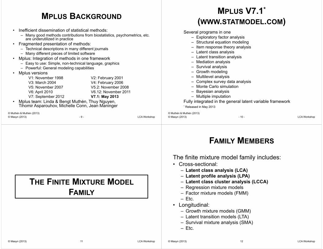
MPLUS BACKGROUND

• Inefficient dissemination of statistical methods:– Many good methods contributions from biostatistics, psychometrics, etc.

are underutilized in practice• Fragmented presentation of methods:

– Technical descriptions in many different journals– Many different pieces of limited software

• Mplus: Integration of methods in one framework– Easy to use: Simple, non-technical language, graphics– Powerful: General modeling capabilities

• Mplus versionsV1: November 1998 V2: February 2001V3: March 2004 V4: February 2006V5: November 2007 V5.2: November 2008V6: April 2010 V6.12: November 2011V7: September 2012 V7.1: May 2013

• Mplus team: Linda & Bengt Muthén, Thuy Nguyen, Tihomir Asparouhov, Michelle Conn, Jean Maninger


MPLUS V7.1*

(WWW.STATMODEL.COM)Several programs in one

– Exploratory factor analysis– Structural equation modeling– Item response theory analysis– Latent class analysis– Latent transition analysis– Mediation analysis– Survival analysis– Growth modeling– Multilevel analysis– Complex survey data analysis– Monte Carlo simulation– Bayesian analysis– Multiple imputation

Fully integrated in the general latent variable framework* Released in May 2013


THE FINITE MIXTURE MODELFAMILY

11© Masyn (2013) LCA Workshop

FAMILY MEMBERS

The finite mixture model family includes:• Cross-sectional:

– Latent class analysis (LCA)– Latent profile analysis (LPA)– Latent class cluster analysis (LCCA)– Regression mixture models– Factor mixture models (FMM)– Etc.

• Longitudinal:– Growth mixture models (GMM)– Latent transition models (LTA)– Survival mixture analysis (SMA)– Etc.


LATENT CLASS ANALYSIS –CATEGORICAL LV AND CATEGORICAL MVS

c

y

u

x T


LATENT PROFILE ANALYSIS/LATENT CLASSCLUSTER ANALYSIS – CATEGORICAL LV AND

CONTINUOUS MVS

c

y

u

x T


FINITE MIXTURE MODEL LIKELIHOOD

• The basic finite mixture model has the following likelihood function:

• K is the number of latent classes• is the proportion of the total population

belonging to Class k.• is the class-specific density function for

the latent class indicator (manifest) variables with class-specific parameters, .


LATENT CLASS ANALYSIS (LCA)

© Masyn (2013) 16 LCA Workshop

17

c

u1 u2 u3 u4

© Masyn (2013) LCA Workshop 18

• Categorical indicators• Categorical latent variable• Cross-sectional data• Some consider LCA the categorical analogue

to factor analysis. • Sometimes referred to as person-centered

analysis to stand in contrast to variable-centered analysis such as CFA.

• Different from IRT that models categorical variables as indicators of an underlying continuous trait (ability).

TRADITIONAL LCA

© Masyn (2013) LCA Workshop

19

• Binary test items as multiple indicators for an underlying 2-level categorical latent variable representing profiles of Mastery and Non-mastery.

• DSM-VI symptom checklist (diagnostic criteria) for depression.

FOR EXAMPLE


StudentItem 1 Item 2 Item 3 Item 4

1 1 1 1 12 0 0 0 03 1 0 1 04 1 0 0 05 0 0 1 06 1 1 1 07 1 1 1 0

EXAMPLE DATA


21

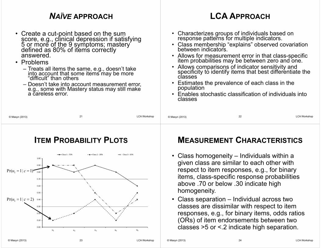
• Create a cut-point based on the sum score, e.g., clinical depression if satisfying 5 or more of the 9 symptoms; mastery defined as 80% of items correctly answered.

• Problems– Treats all items the same, e.g., doesn’t take

into account that some items may be more “difficult” than others

– Doesn’t take into account measurement error, e.g., some with Mastery status may still make a careless error.

NAÏVE APPROACH

© Masyn (2013) LCA Workshop 22

• Characterizes groups of individuals based on response patterns for multiple indicators.

• Class membership “explains” observed covariation between indicators.

• Allows for measurement error in that class-specific item probabilities may be between zero and one.

• Allows comparisons of indicator sensitivity and specificity to identify items that best differentiate the classes

• Estimates the prevalence of each class in the population

• Enables stochastic classification of individuals into classes

LCA APPROACH


ITEM PROBABILITY PLOTS


MEASUREMENT CHARACTERISTICS

• Class homogeneity – Individuals within a given class are similar to each other with respect to item responses, e.g., for binary items, class-specific response probabilities above .70 or below .30 indicate high homogeneity.

• Class separation – Individual across two classes are dissimilar with respect to item responses, e.g., for binary items, odds ratios (ORs) of item endorsements between two classes >5 or <.2 indicate high separation.


ITEM PROBABILITY PLOTS

25© Masyn (2013) LCA Workshop 26

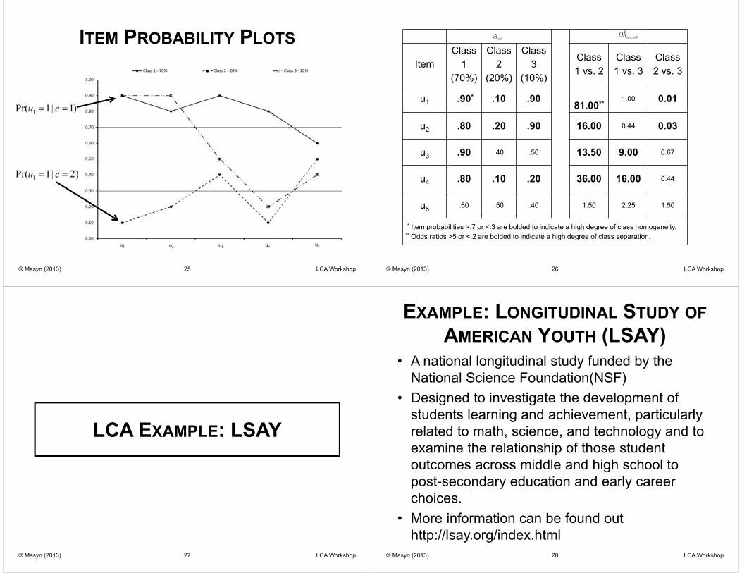
ItemClass

1 (70%)

Class 2

(20%)

Class 3

(10%)

Class 1 vs. 2

Class 1 vs. 3

Class 2 vs. 3

u1 .90* .10 .90 81.00**1.00 0.01

u2 .80 .20 .90 16.00 0.44 0.03

u3 .90 .40 .50 13.50 9.00 0.67

u4 .80 .10 .20 36.00 16.00 0.44

u5 .60 .50 .40 1.50 2.25 1.50

* Item probabilities >.7 or <.3 are bolded to indicate a high degree of class homogeneity.** Odds ratios >5 or <.2 are bolded to indicate a high degree of class separation.


LCA EXAMPLE: LSAY


EXAMPLE: LONGITUDINAL STUDY OFAMERICAN YOUTH (LSAY)

• A national longitudinal study funded by the National Science Foundation(NSF)

• Designed to investigate the development of students learning and achievement, particularly related to math, science, and technology and to examine the relationship of those student outcomes across middle and high school to post-secondary education and early career choices.

• More information can be found out http://lsay.org/index.html


LCA EXAMPLE: LSAY

• Research Aim:– Characterize population heterogeneity in math

attitudes (manifest in 9 survey items) using latent classes of math dispositions.

• Why not state research questions like:– Are there different profiles of math

dispositions based on the math attitude items?

– How many profiles are there?– What are the profiles?

29© Masyn (2013) LCA Workshop 30

Survey Prompt:“Now we would like you to tell us how you feel about math and science. Please indicate for you feel about each of the following statements.”

Total sample (nT = 2675)

f rf

1) I enjoy math. 1784 .67

2) I am good at math. 1850 .69

3) I usually understand what we are doing in math. 2020 .76

4) Doing math often makes me nervous or upset. 1546 .59

5) I often get scared when I open my math book see a page of problems.

1821 .69

6) Math is useful in everyday problems. 1835 .70

7) Math helps a person think logically. 1686 .64

8) It is important to know math to get a good job. 1947 .74

9) I will use math in many ways as an adult. 1858 .70


Usevariables = ca28ar ca28br ca28cr ca28er ca28gr ca28hr ca28ir ca28kr ca28lr;

CATEGORICAL = ca28ar ca28br ca28cr ca28er ca28gr ca28hr ca28ir ca28kr ca28lr;

missing=all(9999);classes= c(5);

Analysis:type=mixture;starts=500 100;processors=4;

Model:Next slide


Model:%overall%[ ca28ar$1 ca28br$1 ca28cr$1 ca28er$1 ca28gr$1 ca28hr$1 ca28ir$1 ca28kr$1 ca28lr$1 ];

%c#1%[ ca28ar$1 ca28br$1 ca28cr$1 ca28er$1 ca28gr$1 ca28hr$1 ca28ir$1 ca28kr$1 ca28lr$1 ];

%c#2%[ ca28ar$1 ca28br$1 ca28cr$1 ca28er$1 ca28gr$1 ca28hr$1 ca28ir$1 ca28kr$1 ca28lr$1 ];

.

.

.%c#5%[ ca28ar$1 ca28br$1 ca28cr$1 ca28er$1 ca28gr$1 ca28hr$1 ca28ir$1 ca28kr$1 ca28lr$1 ];


Note: With categorical indicators, the

following model statement would

produce the same result!

Model:

LCA EXAMPLE: LSAY

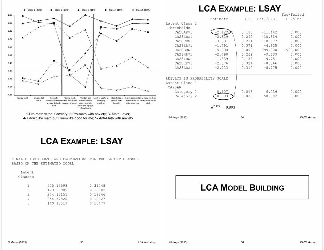
1-Pro-math without anxiety; 2-Pro-math with anxiety; 3- Math Lover; 4- I don’t like math but I know it’s good for me; 5- Anti-Math with anxiety

LCA EXAMPLE: LSAY

34

Two-TailedEstimate S.E. Est./S.E. P-Value

Latent Class 1Thresholds

CA28AR$1 -2.122 0.185 -11.442 0.000CA28BR$1 -2.539 0.242 -10.514 0.000CA28CR$1 -3.081 0.291 -10.577 0.000CA28ER$1 -1.791 0.371 -4.825 0.000CA28GR$1 -15.000 0.000 999.000 999.000CA28HR$1 -2.498 0.262 -9.533 0.000CA28IR$1 -1.839 0.188 -9.781 0.000CA28KR$1 -2.876 0.324 -8.866 0.000CA28LR$1 -2.723 0.310 -8.775 0.000

RESULTS IN PROBABILITY SCALELatent Class 1CA28AR

Category 1 0.107 0.018 6.039 0.000Category 2 0.893 0.018 50.392 0.000


LCA EXAMPLE: LSAY

35

FINAL CLASS COUNTS AND PROPORTIONS FOR THE LATENT CLASSESBASED ON THE ESTIMATED MODEL

LatentClasses

1 525.13598 0.392482 173.96909 0.130023 244.13155 0.182464 254.57820 0.190275 140.18517 0.10477


LCA MODEL BUILDING


MIXTURE MODEL BUILDING STEPS

1. Data screening and descriptives.2. Class enumeration process.3. Select final unconditional model (this is

your measurement model).4. Add potential predictors (and check for

measurement invariance).5. Add potential distal outcomes.


DIRECT AND INDIRECTAPPLICATIONS


DIRECT VS. INDIRECT APPLICATION

y

c

Is the “Truth” a heterogeneous population composed of a mixture of two normally-distributed homogeneous subpopulations?Is the “Truth” a single, non-normally-distributed homogeneous population?


DIRECT APPLICATIONS OF MIXTUREMODELING

• Mixture models are used with the a priori assumption that the overall population is heterogeneous, and made up of a finite number of (latent and substantively meaningful) homogeneous groups or subpopulations, usually specified to have tractable distributions of indicators within groups, such as a multivariate normal distribution.


INDIRECT APPLICATIONS OF MIXTUREMODELING

• It is assumed that the overall population is homogeneous and finite mixtures are simply used as more tractable, semi-parametric technique for modeling a population of outcomes for which it may not be possible (practically- or analytically-speaking) to specify a parametric model.

• The focus for indirect applications is then not on the resultant mixture components nor their interpretation, but rather on the overall population distribution approximated by the mixing.


MODEL ESTIMATION


ML ESTIMATION FOR LCA

• c is treated as missing data under MAR.

• MAR assumes that the probabilities of values being missing are independent of the missing values conditional on those values that are observed (both u and x). (Little and Rubin, 2002)


• Basic principle of ML: Choose estimates of the model parameters whose values, if true, would maximize the probability of observing what had, in fact, been observed.

• This requires an expression that describes the distribution of the data as a function of the unknown parameters, i.e., the likelihood function.


• Under MAR, the ML estimates for the complete data may be obtained by maximizing the likelihood function summed over all possible values of the missing data, i.e., integrate out the missingness.

• Often, this integrated likelihood cannot be maximized analytically and requires an iterative estimation procedure, e.g., EM.


THE EM ALGORITHM

• How does it work?– Start with random split of people into classes. – Reclassify based on a improvement criterion– Reclassify until the “best” classification of

people is found.• The EM algorithm is a missing data

technique. In this application, the latent class variable is the missing data– and it happens to be missing for the entire data set.


ML ESTIMATION VIA EM ALGORITHM

E(xpectation) step: c is treated as missing data. Missing values ci are replaced by the conditional means of cigiven the yi’s. These means are the posterior probabilities for each class.

M(aximization) step: New estimates of the parameters are obtained from the maximization based on the estimated complete-data. Pr(yj|c=k) and Pr(c=k) parameters are estimated by regression and summation over the posterior probabilities.

• Missing data is allowed on the y’s as well, assuming MAR.

• Standard errors are obtained using some approximation to the Fisher information matrix. (In Mplus, “ML” default for no missing data on the y’s; “MLR” for missing data on indicators).


THE CHALLENGES OF ML VIA EM• MLE for mixture models can present

statistical and numeric challenges that must be addressed during the application of mixture modeling:– The estimation may fail to converge even if

the model is theoretically identified.– If the estimation algorithm does converge,

since the log likelihood surface for mixtures is often multimodal, there is no way to prove the solution is a global rather than local maximum.


© Masyn (2013) 49 LCA Workshop © Masyn (2013) 50 LCA Workshop

How would you distinguish between these two cases?

MOST IMPORTANTLY: • Use multiple random sets of starting values with the

estimation algorithm—it is recommended that a minimum of 50 to 100 sets of extensively, randomly varied starting values are used (Hipp & Bauer, 2006) but more may be necessary to observe satisfactory replication of the best maximum log likelihood value.

• Recommendations for a more thorough investigation of multiple solutions when there are more than two classes:ANALYSIS: STARTS = 50 5;or with many classesANALYSIS: STARTS = 500 10


Note: LL replication is neither necessary or sufficient for a given solution to be the global maximum.


And keep track of the following information:• The number and proportion of sets of random starting values

that converge to proper solution (as failure to consistently converge can indicate weak identification);

• The number and proportion of replicated maximum likelihood values for each local and the apparent global solution (as a high frequency of replication of the apparent global solution across the sets of random starting values increases confidence that the “best” solution found is the true maximum likelihood solution);

• The condition number. It is computed as the ratio of the smallest to largest eigenvalue of the information matrix estimate based on the maximum likelihood solution. A low condition number, less than 10-6, may indicate singularity (or near singularity) of the information matrix and, hence, model non-identification (or empirical underidentification)

• The smallest estimated class proportion and estimated class size among all the latent classes estimated in the model (as a class proportion near zero can be a sign of class collapsing and class over-extraction).


• This information, when examined collectively, will assist in tagging models that are non-identified or not well-identified and whose maximum likelihoods solutions, if obtained, are not likely to be stable or trustworthy. These not well-identified models should be discarded from further consideration or mindfully modified in such a way that the empirical issues surrounding the estimation for that particular model are resolved without compromising the theoretical integrity and substantive foundations of the analytic model.


CLASS ENUMERATION


NOW THE HARD PART • In the majority of applications of mixture

modeling, the number of classes is not known.

• Even in direct applications, when one assumes a priori that the population is heterogeneous, you rarely have specific hypotheses regarding the exact number or nature of the subpopulations.

• Thus, in either case (direct or indirect), you must begin with the model building with an exploratory class enumeration step.


• Deciding on the number of classes is often the most arduous phase of the mixture modeling process.

• It is labor intensive because it requires consideration (and, therefore, estimation) of a set of models with a varying numbers of classes

• It is complicated in that the selection of a “final” model from the set of models under consideration requires the examination of a host of fit indices along with substantive scrutiny and practical reflection, as there is no single method for comparing models with differing numbers of latent classes that is widely accepted as best.


EVALUATING THE MODEL

The statistical tools are divided into three categories: 1. evaluations of

absolute fit; 2. evaluations of

relative fit; 3. evaluations of

classification.

Model Usefulness• Substantive meaningful

and substantively distinct classes (face + content validity)

• Cross-validation in second sample (or split sample)

• Parsimony principle• Criterion-related validity


CLASS ENUMERATION PROCESS FOR LCA

• Fit models for K=1, 2, 3, increasing K until the models become not well-identified.

• Collect fit information on each model using a combination of statistical tools

• Decide on 1-2 “plausible” models • Apply broader set of statistical tools to set

of candidate models and evaluate the model usefulness.


FIT INDICES


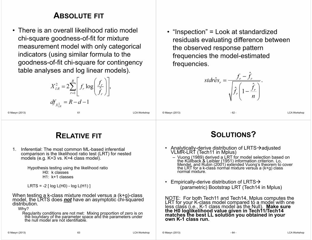
ABSOLUTE FIT

• There is an overall likelihood ratio model chi-square goodness-of-fit for mixture measurement model with only categorical indicators (using similar formula to the goodness-of-fit chi-square for contingency table analyses and log linear models).


• “Inspection” = Look at standardized residuals evaluating difference between the observed response pattern frequencies the model-estimated frequencies.


RELATIVE FIT

1. Inferential: The most common ML-based inferential comparison is the likelihood ratio test (LRT) for nested models (e.g. K=3 vs. K=4 class model).

Hypothesis testing using the likelihood ratioH0: k classesH1: k+1 classes

LRTS = -2 [ log L(H0) - log L(H1) ]

When testing a k-class mixture model versus a (k+g)-class model, the LRTS does not have an asymptotic chi-squared distribution.

Why?Regularity conditions are not met: Mixing proportion of zero is on

the boundary of the parameter space and the parameters under the null model are not identifiable.


SOLUTIONS?• Analytically-derive distribution of LRTS adjusted

VLMR-LRT (Tech11 in Mplus)– Vuong (1989) derived a LRT for model selection based on

the Kullback & Leibler (1951) information criterion. Lo, Mendel, and Rubin (2001) extended Vuong’s theorem to cover the LRT for a k-class normal mixture versus a (k+g) class normal mixture.

• Empirically-derive distribution of LRTS(parametric) Bootstrap LRT (Tech14 in Mplus)

NOTE: For both Tech11 and Tech14, Mplus computes the LRT for your K-class model compared to a model with one less class (i.e., K-1 class model as the Null). Make sure the H0 loglikelihood value given in Tech11/Tech14 matches the best LL solution you obtained in your own K-1 class run.


2. Information-heuristic criteria: These indices weigh the fit of the model (as captured by the maximum log likelihood value) in consideration of the model complexity (recognizing that although one can always improve the fit of a model by adding parameters, there is a cost that improvement in fit to model parsimony).

• These information criteria can be expressed in the following form:

• Traditional penalty is a function of n and d; n= sample size, d= number of parameters


INFORMATION CRITERIA

• Bayesian Information Criterion

• Consistent Akaike’s Information Criterion

• Approximate Weight of Evidence Criterion

• For these ICs, lower values indicate a better model, relatively-speaking. Sometime, a minimum values if not reached and scree/”elbow” plots are utilized.


How much lower does an IC values have to be to mean the model is really better?• Bayes Factor: Which model, A or B, is

more likely to be the true model if one of the two is the true model?


• The approximate correct model probability (cmP) for a Model A is an approximation of the actual probability of Model A being the correct model relative to a set of J models under consideration .



CLASSIFICATION QUALITY


CLASSIFICATION QUALITY/CLASSSEPARATION

• A good mixture model in a direct application* should yield empirically, highly-differentiated, well-separated latent classes whose members have a high degree of homogeneity in their responses on the class indicators.

*A well-fitting mixture model can have very poor class separation Classificationquality is not a measure of model fit!


• Most all of the classification diagnostics are based on estimated posterior class probabilities.

• Posterior class probabilities are the model-estimated values for each individual’s probabilities of being in each of the latent classes based on the maximum likelihood parameter estimates and the individual’s observed responses on the indicator variables (similar estimated factor scores).


RELATIVE ENTROPY

• An index that summarizes the overall precision of classification for the whole sample across all the latent classes

• When posterior classification is no better than random guessing, E=0, and when there is perfect posterior classification for all individuals in the sample, E=1.


• Since even when E is close to 1.00 there can be a high degree of latent class assignment error for particular individuals, and since posterior classification uncertainty may increase simply by chance for models with more latent classes, E was never intended nor should it be used for model selection during the class enumeration process. (REMEMBER: A mixture model with low entropy could still fit the data well.)

• However, values near zero may indicate that the latent classes are not sufficiently well-separated for the classes that have been estimated. Thus, E may be used to identify problematic over-extraction of latent classes and may also be used to judge the utility of the latent class analysis directly applied to a particular set of indicators to produce empirically, highly-differentiated groups in the sample.


AVEPP• Average posterior class probability (AvePP),

enables evaluation of the classification uncertainty for each of the latent classes separately.

• The average posterior class probability for each class, k, among all individuals whose maximum posterior class probability is for Class k (i.e., individuals modally assigned to Class k).

• Nagin suggests AvePP values >.7 indicate adequate separation and classification precision.


OCC

• The denominator of the odds of correct classification (OCC) is the odds of correct classification based on random assignment using the model-estimated marginal class proportions.

• The numerator is the odds of correct classification based on the maximum posterior class probability assignment rule (i.e., modal class assignment).

• When the modal class assignment for Class k is no better than chance, then OCC(k)=0.

• As AvePP(k) gets close to one, OCC(k) gets large.• Nagin suggests OCC(k)>5 indicate adequate separation and

classification precision.


MCAP• Modal class assignment proportion (mcaP) is

the proportion of individuals in the sample modally-assigned to Class k.

• If individuals were assigned to Class k with perfect certainty, then mcaP(k) would be equal to the model-estimated Pr(c=k). Larger discrepancies are indicative of larger latent class assignment errors.

• To gauge the discrepancy, each mcaP can be compared to the to 95% confidence interval for the corresponding model-estimated Pr(c=k).

© Masyn (2013) LCA Workshop- 77 - © Masyn (2013) LCA Workshop- 78 -

SUMMING IT UP


1)

2)


3)


4)

5)


5a)


5b)


5c)


5d)

5e)

6)


AND, FINALLY

• On the basis of all the comparisons made in Steps 5 and 6, select the final model in the class enumeration process. – Note: You may end up carrying forward two

candidate models into the conditional modeling stage.

• If you had a large enough sample to do a split-half cross-validation, now is when you would look at the validation sample.


7)

LATENT CLASS REGRESSION(LCR)


LATENT CLASS VALIDATION

• Link the conceptual/theoretical aspects of the latent class variable with observable variables

• “[To] make clear what something is” means to set forth the laws in which it occurs

• Cronbach & Meehl (1955) termed this process the nomological (or lawful) network


LINKAGES CRITERION-RELATED VALIDITY• In criteria-related validity (concurrent and

predictive), we check the performance of our latent classes against some criterion based on our theory of the construct represent by the latent class variable. – Concurrent: Latent class membership predicted

by or covarying with past or concurrent events (Latent class regression)

– Predictive: Latent class membership predicting future concrete events (Latent class w/ distal outcomes).


COVARIATES AND MIXTURE MODELS

u1 u2 u3 u4 u5

CRisk Factor

Indirect Effect

Direct effect


LATENT CLASS REGRESSION

• Like a MIMIC model in regular CFA/SEM• Categorical latent variable• Continuous or categorical covariates with

direct effects on y’s or indirect effects on y’s through c. – Indirect effects can also be thought of as

predictors of class membership. – Direct effects can also be thought of as

differential item functioning.


INCLUDING COVARIATES INTO LCA

• The inclusion of covariates into mixture models– Allow us to explore relationships of mixture

classes and auxiliary information.

– Understand how different classes relate to risk and protective factors

– Explore differences in demographics across the classes

© Masyn (2013) LCA Workshop94

“C ON X” = MULTINOMIAL REGRESSION

• Multinomial logistic regression is essentially simultaneous pairs of logistic regression of the odds in each outcome category versus a reference/baseline category.

• Mplus uses the last category/class as the baseline.

• So for K classes, we have K-1 logit equations.

© Masyn (2013) LCA Workshop95

• We model the following: Given membership in either Class k or K, what is the log odds that class membership is k (instead of K), given x? That is,


I enjoy Math I am good at math

I will use math later. . .

Male C

LSAY EXAMPLE

MODEL:%Overall% c on male;


LCA EXAMPLE: LSAY

1-Pro-math without anxiety, 2-Pro-math with anxiety, 3- Math Lover, 4- I don’t like math but I know it’s good for me, 5- Anti-Math with anxiety

EXAMPLE: LSAY WITH COVARIATECategorical Latent Variables*C#1 ON

FEMALE 0.320 0.217 1.476 0.140C#2 ON

FEMALE -0.343 0.269 -1.274 0.203C#3 ON

FEMALE 0.485 0.266 1.823 0.068C#4 ON

FEMALE 0.865 0.258 3.356 0.001

*Class 5 is reference group

There is a statistically significant overall association with gender and math deposition: - Null Model (no effect of female) vs. Alt. Model (c on female):

, df = 4, p<.001) - Interpretation of coefficients:- Given membership in either Class 1 or 5, girls are as likely to be in Class 1 as boys

(p=.14).- Given membership in either Class 2 or 5, girls are as likely to be in Class 2 as boys

(p=.20). - Etc.


EXAMPLE: LSAY WITH COVARIATE

ALTERNATIVE PARAMETERIZATIONS FOR THE CATEGORICAL LATENT VARIABLE REGRESSION

Parameterization using Reference Class 1

C#2 ONFEMALE -0.662 0.205 -3.223 0.001

C#3 ONFEMALE 0.165 0.207 0.798 0.425

C#4 ONFEMALE 0.545 0.187 2.916 0.004

C#5 ONFEMALE -0.320 0.217 -1.476 0.140

100

Switching the reference group to Class 1:

© Masyn (2013)


LCA Workshop

EXAMPLE: LSAY WITH COVARIATE


“1-STEP” APPROACH FORLATENT CLASS PREDICTORS


LCR MODELING PROCESS1. Fit models without covariates first.2. Decide on the number of classes.3. Integrate covariate (indirect) effects in a

systematic way. (You can preview covariate, x, using auxiliary = x (r) or (r3step) option in Variable command.) Include indirect effects (class predictors) first with direct effects @0 and then explore the evidence for direct effects using modindices.

4. Add direct effects as suggest by modindices but do not vary across class.

5. Trim until only significant direct effects remain.NOTE: This is just like MIMIC modeling in SEMAlso NOTE: There are other approaches currently in development for detection of direct effects and DIF more generally.


WHY NOT ADD CLASS-VARYINGDIRECT EFFECTS?

u1 u2 u3 u4 u5

C

Indirect Effect;Mplus:%overall%C on X;

Direct effect:%overall%U4 on X; Class-varying Direct Effect:

%c#1%U4 on X;

%c#2%U4 on X;

104

Covariate


“OLD” 3-STEP APPROACH FORLATENT CLASS PREDICTORS


• Estimate the LCA model• Determine each subject’s most likely class

membership (“hard” classify people using modal class assingment)

• Save the class assignment and use in separate analysis as observed multinomial outcome to relate predictors to class membership.

• Problematic: Unless the classification is very good (high entropy), this gives biased estimates and biased standard errors for the relationships of class membership with other variables.


NEW 3-STEP APPROACH FORLATENT CLASS PREDICTORS


BASIC IDEA

• The real problem with the classify-analyze (“old” 3-step approach) is that it ignores the uncertainly/imprecision in classification.

• Based on the results of the unconditional LCA, we can compile information about classification quality that we can then use in a subsequent model (akin to using a previously estimated scale reliability to specify the measurement error variance in an SEM model).– The information is summarized in: Logits for the

Classification Probabilities for Most Likely Class Membership (Row) by Latent Class (Column)


• Average Latent Class Probabilities for Most Likely Latent Class Membership (Row) by Latent Class (Column) estimates

Pr(C = j | CMOD = k) for j=1, ,K, k=1, ,K• Classification Probabilities for the Most Likely

Latent Class Membership (Row) by Latent Class (Column) estimates

Pr(CMOD = k | C = j) for j=1, ,K, k=1, ,K• How do you get from one quantity to the

others? Bayes' Theorem:


1. Estimate the LCA model2. Create a nominal most likely class variable,

CMOD3. Use a mixture model for CMOD, C, and X,

where CMOD is the nominal indicator of C with measurement error rates prefixed at the misclassification rates of the estimated model in the step 1 LCA.

The information is summarized in: Logits of Average Latent Class Probabilities for Most Likely Class Membership (Row) by Latent Class (Column)

To do this in Mplus for X, use auxiliary = X (r3step) option in Variable command.



CMOD

X

C

Fixed according to Step 1 misclassification rates

Estimated

MANUAL R3STEPSTEP 1:• Run model with covariate(s) as auxiliary variable.

Include SAVEDATA:File is step1save.dat;SAVE=CPROB;

STEP 2:• Create new input file using

DATA:File is step1save.dat;VARIABLE:UseVar = cmod x;Nominal = cmod;


• Use value from the rows of the Logits for the Classification Probabilities for the Most Likely Latent Class Membership (Row) by Latent Class (Column) table in Step 1 output to fix the class-specific multinomial intercepts for cmod.

Step 3:• Specify LCR of “c on x” and run.


DISTAL OUTCOMES


DISTAL OUTCOMES AND MIXTUREMODELS

Distal Outcome

u1 u2 u3 u4 u5

C


AN EVER-GROWING # OF APPROACHES

• 1-step• “Old” 3-step (classify-analyze)• Modified 1-step• Pseudo-class draws

– Auxiliary = z (E);• New 3-step

– Auxiliary = z (DU3step) or (DE3step)– Manual 3-step

• New Bayes’ Theorem approach by Lanza et al. (2013)– Auxiliary = z (DCON) or (DCAT)


1-STEP

• Also referred to as the “distal-as-indicator” approach.

• Distal is treated as an additional latent class indicator if included as endogenous variable– This means you latent class variable is now

specified as measured by all the items andthe distals.

– This may be what you intend but, if so, the distals should be included as indicators from the get-go.


NOT GOOD OR BAD, JUST MAYBE NOTWHAT YOU WANT

• What if you don’t want your distal outcomes to characterized/measure the latent class variable?

• All the other existing approaches are an attempt to keep the distal outcome from influencing the class formation.


ALTERNATIVES TO DISTAL-AS-INDICATOR

• Old 3-step has the same problems as it does for latent class regression

• Modified 1-step fixes all measurement parameters (e.g., item thresholds) at their estimated values from the unconditional model.


• New 3-step– Done the same as for the LCR. Mplus will test for

differences in means assuming equal variances (DE3step) or allowing unequal variances (DU3step).

– Mplus implementation is limited but you can always do a manual 3-step in order to analyze multiple distal outcomes at the same time while including covariates, potential moderators, etc.

– WARNING: The 3-step approach does not guarantee that your distal will not influence the latent class formation. Mplus checks for this now—you have to check yourself if using manual 3-step.


AUXILIARY = Z (DCON/DCAT)• Based on clever application of Bayes’ Theorem by

Lanza et al. (2013)

• Basic idea: Regress C on Z to obtain Pr(C|Z) and Pr(C), estimate the density function of Z for Pr(Z) and then apply Bayes’ Theorem to get Pr(Z|C).

• This technique does better w.r.t. not allowing Z to influence class formation, but is very limited w.r.t. to the structural models that can be specified (e.g., one distal at a time, must assume distal independent of covariates, etc.)


MIXTURE MODEL BUILDING STEPS

1. Data screening (and unconditional, saturated non-mixture model if applicable)

2. Class enumeration process (without covariates)a) Enumeration (within each k structure if applicable)b) Comparisons of most plausible models from (a).NOTE: You may end up going through this step multiple times as you may realize to need to modify or reconsider your set of class indicators.

3. Select final unconditional model.4. Add potential predictors; Consider both prediction

of class membership and also possibly measurement non-invariance/DIF

5. Conditional mixture model with distal outcomes: Add potential distal outcomes of class membership.


MODELING EXTENSIONS


PREDICTORS AND DISTALS= LC MEDIATION!


REGRESSION MIXTURE MODELS


HIGHER-ORDER LATENT CLASS

C1 C3C2

C


MULTIPLE GROUP LCA(USES KNOWNCLASS OPTION)

C1

CG


MULTILEVEL LCA


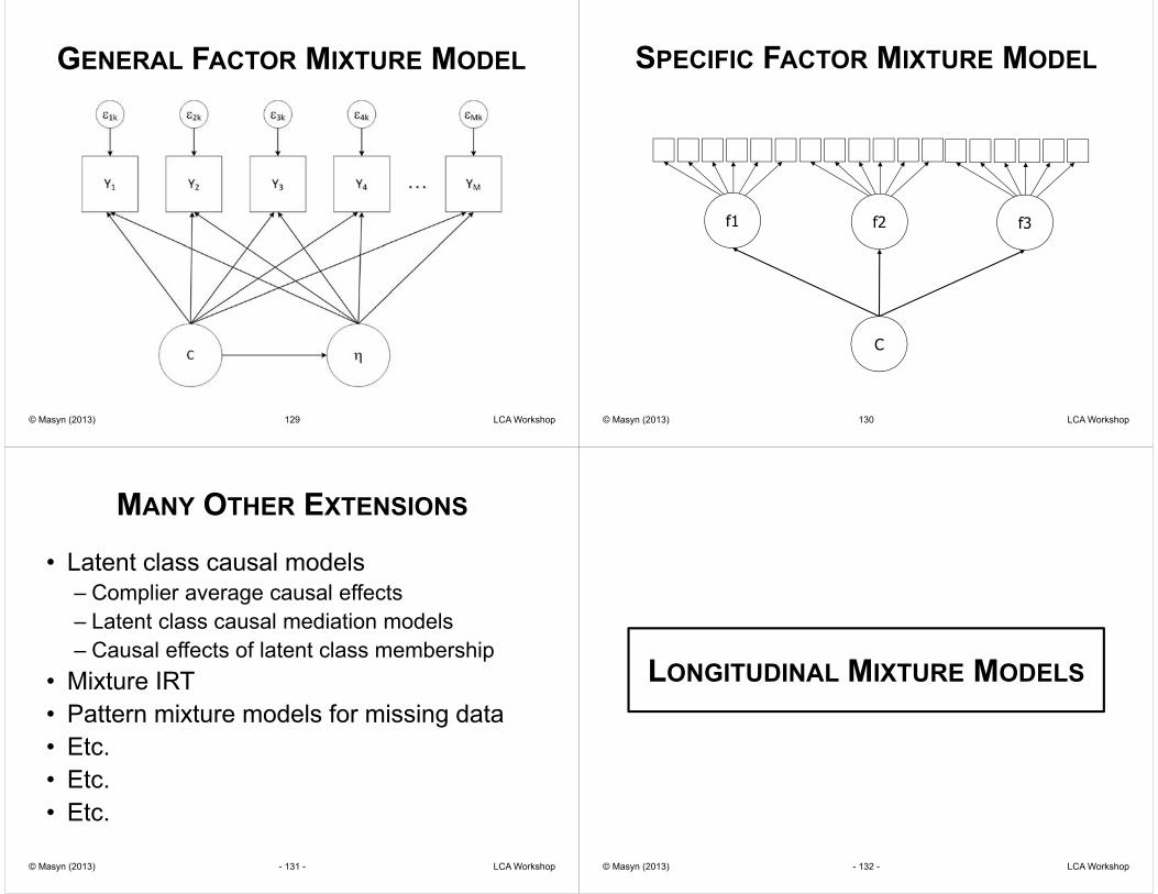
GENERAL FACTOR MIXTURE MODEL


f1 f3f2

C


SPECIFIC FACTOR MIXTURE MODEL

MANY OTHER EXTENSIONS

• Latent class causal models– Complier average causal effects– Latent class causal mediation models– Causal effects of latent class membership

• Mixture IRT• Pattern mixture models for missing data• Etc.• Etc.• Etc.


LONGITUDINAL MIXTURE MODELS


LONGITUDINAL LCA (LLCA) / RMLCA


LONGITUDINAL LCA

• Use latent class variable to characterize longitudinal response patterns.

• The EXACT same modeling process as for LCA/LPA!

• The EXACT same syntax in Mplus.– The only differences is that in your data, u1-

uM or y1-yM are single variables measured at multiple time points rather than multiple measures at single time point.


GROWTH MIXTURE MODELS


c

10

Y 2Y 1 Y 3 Y 4

x

u

z

GENERAL GROWTH MIXTURE MODEL (GGMM)

AGGRESSION DEVELOPMENT: CONTROL AND INTERVENTION GROUPS

LATENT TRANSITION ANALYSIS (LTA)


C2=1 C2=2 C2=3

C1=1 Pr(1 1) Pr(1 2) Pr(1 3)

C1=2 Pr(2 1) Pr(2 2) Pr(2 3)

C1=3 Pr(3 1) Pr(3 2) Pr(3 3)

Time 1

Time 2

- 139 -

LTA• Begin with LCA/LPA models for each time

point separately. Use the same exact modeling process as for a single cross-sectional LCA/LPA.

• Bring the latent class variables together in a single model. Watch for label switching and actual changes in measurement model parameters at each wave with all time points in same model.– There is a LTA 3-Step. See NEW Webnote 15 for

more information• Bring in covariates and distal outcomes using

same approaches as for LCA/LPA.© Masyn (2013) LCA Workshop- 140 -


LTA with predictors that influence not only class membership at each time point but the transitions as well.

Here’s how you have to specify that in Mplus. You can rearrange results to address questions posed by model above.

MANY OTHER LONGITUDINALMIXTURE MODELS

• Survival mixture models• Latent change score mixture models• Onset-to-growth mixture models• Associative LTA• Latent transition growth mixture models• Etc.• Etc.• Etc.


PARTING WORDS


MIXTURE MODELS: LAUDED BY SOME

• Theoretical models that conceptualize individual differences at the latent level as differences in kind, that consider typologies or taxonomies, map directly onto analytic latent class models.

• Mixture models give us a great deal of flexibility in terms of how we characterize population heterogeneity and individual differences with respect to a latent phenomenon.

• Can help avoid serious distortions that can results from ignoring population heterogeneity if it is, indeed, present.


MIXTURE MODELS: IMPUGNED BY OTHERS

• Latent classes or mixtures may not reflect the Truth.

• Nominalistic fallacy: Naming the latent classes does not necessarily make them what we call them or ensure that we understand them.

• Reification: Just because the model yield latent classes doesn’t mean the latent classes are real or that we’ve done anything to prove their existence.


• The empirically extracted latent classes depend upon the within- and between-class model specification and the joint distribution of the indicators. Thus, the resultant classes may diverge markedly from the underlying “True” latent structure in the population.

• Do these criticisms sound familiar? They are nearly identical to the critique of path analysis and SEM in the second half of the 20th century because some of the same bad modeling practices have reappeared:– “Nobody pays much attention to the

assumptions, and the technology tends to overwhelm common sense.” (Friedman, 1987)


DON’T CUT OFF YOUR LATENT CLASSESTO SPITE YOUR MODEL

• Any model is, at best, an approximation to reality.• “All models are wrong, but some are useful”. (George

Box)• We can evaluate model-theory consistency. • We can evaluate model-data consistency. • There are many alternative ways of thinking about

relationships in a variable system and if mixture modeling can be useful in empirically distinguishing between or among alternative perspectives, then they provide important information.


• Understanding individual differences is paramount in social and developmental research.

• The flexibility we gain in the parameterization of individual differences using mixtures extends to flexibility in prediction of those differences and prediction from those differences.


MIXTURE MODEL CARE AND FEEDING• Be sure to very carefully document your model building and

selection for yourself and reviewers. Be prepared to defend your modeling choices in the event you get a reviews that is more skeptical than most about the methodology.

• Resist the temptation to take your discrete representation of population heterogeneity and claim and interpret and discuss the resultant classes as if you had established their existence (e.g., if you fit a three class model and you get a three class solution, you haven’t proved the existence of three classes generally nor those three classes specifically).

• In designing studies in which you plan to do LCA/LPA, don’t formulate hypotheses such as “There will be four classes of engagement” because the exploratory class enumeration process doesn’t actually test K=4 versus K 4. This also makes it impossible to compute power.


• Don’t be afraid to do some sensitivity analyses to understand the hierarchy of influence in your variable system and the vulnerability of your latent class formations to small shifts in that system.

• Don’t check your common sense and broader modeling skills at the door when embarking on LCA/LPA. There are some modeling best-practices that translate extremely well to the LCA setting.

• Don’t get so overwhelmed with all the fit indices, etc. that you forget to fully evaluate the substantive utility and meaning in the resultant classes.

• Don’t be so dazzled by your own results that you aren’t able to effective and critically evaluate them with respect to validity criteria.

• Don’t fall so deeply in love with mixture modeling that it becomes your default analytic approach with any multivariate data.


QUESTIONS?

THANK YOU!


SELECT REFERENCES & RESOURCES


• Mplus websitewww.statmodel.com

• Latent GOLD websitehttp://statisticalinnovations.com/products/latentgold.html

• Penn State Methodology Centerhttp://methodology.psu.edu/

• UCLA Institute for Digital Research & Educ.https://idre.ucla.edu/stats

For more, see the text and references of: Masyn, K. (2013). Latent class analysis and finite mixture modeling. In T. D. Little (Ed.) The Oxford handbook of quantitative methods in psychology (Vol. 2, pp. 551-611). New York, NY: Oxford University Press.

APPLIED VIEW YSIS - Texas Tech University€¦ · APPLIED YSIS: Ph.D. University...

Documents

Transcript of APPLIED VIEW YSIS - Texas Tech University€¦ · APPLIED YSIS: Ph.D. University...