Applied Numerical Mathematics - LIRMM

JID:APNUM AID:2865 /FLA [m3G; v 1.137; Prn:25/09/2014; 11:51] P.1 (1-17)

Applied Numerical Mathematics ••• (••••) •••–•••

Contents lists available at ScienceDirect

Applied Numerical Mathematics

www.elsevier.com/locate/apnum

Nonlinear PDE based numerical methods for cell tracking

in zebrafish embryogenesis

Karol Mikula a,∗,1, Róbert Špir a,1, Michal Smíšek a,1, Emmanuel Faure b, Nadine Peyriéras c

a Department of Mathematics, Slovak University of Technology, Radlinskeho 11, 813 68 Bratislava, Slovakiab CREA, École Polytechnique, 32 boulevard Victor, 75015 Paris, Francec Institut de Neurobiologie Alfred Fessard, CNRS UPR 3294, Av. de la Terrasse, 91198 Gif-sur-Yvette, France

a r t i c l e i n f o a b s t r a c t

Article history:Available online xxxx

Keywords:Numerical methodsNonlinear partial differential equationsImage processingCell tracking

The paper presents numerical algorithms leading to an automated cell tracking and reconstruction of the cell lineage tree during the first hours of animal embryogenesis. We present results obtained for large-scale 3D+time two-photon laser scanning microscopy images of early stages of zebrafish (Danio rerio) embryo development. Our approach consists of three basic steps – the image filtering, the cell centers detection and the cell trajectories extraction yielding the lineage tree reconstruction. In all three steps we use nonlinear partial differential equations. For the filtering the geodesic mean curvature flow in level set formulation is used, for the cell center detection the motion of level sets by a constant speed regularized by mean curvature flow is used and the solution of the eikonal equation is essential for the cell trajectories extraction. The core of our new tracking method is an original approach to cell trajectories extraction based on finding a continuous centered paths inside the spatio-temporal tree structures representing cell movement and divisions. Such paths are found by using a suitably designed distance function from cell centers detected in all time steps of the 3D+time image sequence and by a backtracking in the steepest descent direction of a potential field based on this distance function. We also present efficient and naturally parallelizable discretizations of the aforementioned nonlinear PDEs and discuss properties and results of our new tracking method on artificial and real 4D data.

© 2014 IMACS. Published by Elsevier B.V. All rights reserved.

1. Introduction

The development of the modern microscopy techniques allows the in vivo imaging of organisms at cell level at very early stages of development without corrupting the cell integrity and normal development of the embryo. The multi-photon laser scanning microscopy is able to deliver 3D+time images of long periods of the embryonic development with a relatively short time step. With such data, one can perform various analyses of the embryogenesis and the development of organisms. Due to a similarity with human in many aspects and due to transparency for the microscope, the zebrafish (Danio rerio) embryogenesis is studied extensively and the results are used both in basic and applied biology and medicine research, e.g. in the anticancer drug design.

* Corresponding author.1 The authors were supported by the grant APVV-0184-10.

http://dx.doi.org/10.1016/j.apnum.2014.09.0020168-9274/© 2014 IMACS. Published by Elsevier B.V. All rights reserved.

http://www.ScienceDirect.com/

http://www.elsevier.com/locate/apnum

http://dx.doi.org/10.1016/j.apnum.2014.09.002


2 K. Mikula et al. / Applied Numerical Mathematics ••• (••••) •••–•••

Although a large amount of work has been already done, e.g. by a combination of various image processing techniques and manual inspection, for the zebrafish developmental stages up to about one thousand cells [19], there is a great challenge to study embryogenesis at very complex stages of development with thousands of cells present. In [12,22,18,3] new efficient and robust 3D filtering and segmentation algorithms together with a workflow for performing various analyses of such complex developmental stages were suggested and studied. Among other goals, the image processing algorithms aim to deliver the so-called cell lineage tree, the spatio-temporal branching process giving topological description of movement and division of the cells. This problem is related to tracking of cells during the embryogenesis. Having the tree, one can track the cells by following the links in the tree, either forward or backward. On the other hand, having the good cell tracking algorithm and thus individual cell trajectories, one can reconstruct the tree.

The tracking of cells and construction of the cell lineage tree for such complex stages of embryogenesis is a very difficult problem unsolved satisfactorily yet. A seminal work towards building the cell lineage tree for the complex stages of zebrafish embryo development based on stochastic simulated annealing minimization of a heuristic energy functional has been done in [13]. After the construction of the tree, the individual cells or cell populations are tracked. In this paper we suggest new PDE based cell tracking method for such complex stages of zebrafish embryogenesis. In the present work we continue the effort started in [1,17] devoted to 2D+time and 3D+time cells tracking. In contrast to [13], in our approach we first extract all possible cell trajectories inside the 3D+time data and then the cell lineage tree is reconstructed by finding merging trajectories going backward in time.

Our overall approach to cell tracking consists of three basic steps – the image filtering, the cell centers detection and the cell trajectories extraction yielding the cell lineage tree reconstruction. In all three steps we use suitably designed nonlinear partial differential equations – for filtering the geodesic mean curvature flow in level set formulation is used, for cell center detection the motion of level sets by a constant speed regularized by mean curvature flow is used and solution of the eikonal equation is essential for the cell trajectories extraction. We also present efficient and naturally parallelizable discretizations of the aforementioned nonlinear PDEs and discuss properties and results of our new tracking method.

The first step of our technique is the image filtering. This is an important step because noise is always present in microscopy images and its level increases with the speed of image acquisition. We perform the filtering of 3D images of the 3D+time image sequence by the numerical solution of the so-called geodesic mean curvature flow (GMCF) model [5,11,6]which was chosen from several available methods by careful testing [12].

In the second step of our approach we use the level set center detection (LSCD) method [10] to extract an approximate position of the cell nuclei centers (which we also call the cell identifiers) in every 3D image of the 3D+time image sequence. LSCD method is represented by an evolutionary process based on the motion of level sets of 3D image intensity in normal direction by a constant speed regularized by the mean curvature flow. Following the local maxima of the solution during the evolution one can obtain a reasonable approximation of cell nuclei center positions and its number in every 3D image.

The cell identifiers represent the basic input for the third step of the overall tracking procedure, the cell trajectories extraction and the cell lineage tree reconstruction. The cell trajectories are extracted by finding centered paths inside a specifically constructed 4D spatio-temporal tree structure. Although we call it tree structure, it represents a subset of nonzero measure of the Euclidean space R4 and is given by a 4D segmentation step. Thus, in the first step of the trajecto-ries extraction we construct a 4D segmentation yielding the desired 4D spatio-temporal tree structure. Then a computation of constrained distance functions inside this 4D segmentation is performed by solving a spatially 4D eikonal equation. By a proper combination of computed distance functions we build a potential field which is backtracked in the steepest descent direction in order to get the cell trajectories. Finally we construct the cell lineage tree by detecting trajectories which merge together when going backward in time indicating mitosis and thus a branching node of the cell lineage tree.

The paper is organized as follows. In the next subsection we present the zebrafish embryo development data acquired by the two-photon laser scanning microscope. Then we present all three steps of our approach, the image filtering, the cell center detection and the cell trajectories extraction. Together with the PDE based models, we outline the numerical approaches used in all three steps of our tracking method. Finally we discuss the numerical experiment devoted to tracking cells in a representative 3D video of the early zebrafish embryogenesis.

1.1. 3D+time = 4D image data of zebrafish embryogenesis

Data for processing comes from two-photon laser scanning microscopy and they are of general interest, so we present some illustrative examples how it looks like. The data we deal with represents first hours of zebrafish embryo development, approximately from the 4th until 14th–20th hour. Usually, the data comes in two channels (two colors), in one channel there is an acquisition of the cell nuclei and in the second channel the acquisition of the cell membranes. The embryo labeling is obtained through RNA injection performed at the one-cell stage to obtain expression of fluorescence proteins staining nuclei and membranes, respectively. The embryo imaging starts about 4 hours post-fertilization and take next 10–15 hours. The 3D images of both channels are obtained by moving the focal plane from the top more deeply inside the embryo and their quality depend on the speed of scanning in one plane. Many various quality datasets are available thanks to EC Embryomics and BioEmergences projects (http :/ /bioemergences .iscpif .fr). The data quality is related to a level of noise depending mainly on the size of the time step between acquisition of subsequent 3D images. The acquisition step ranges from 50 seconds to 5 minutes. A longer time step produces better 3D image quality, one has a good visual impression of what is happening during embryogenesis and such data is well suited for segmentation purposes e.g. for obtaining a shape of cells and other

http://bioemergences.iscpif.fr


K. Mikula et al. / Applied Numerical Mathematics ••• (••••) •••–••• 3

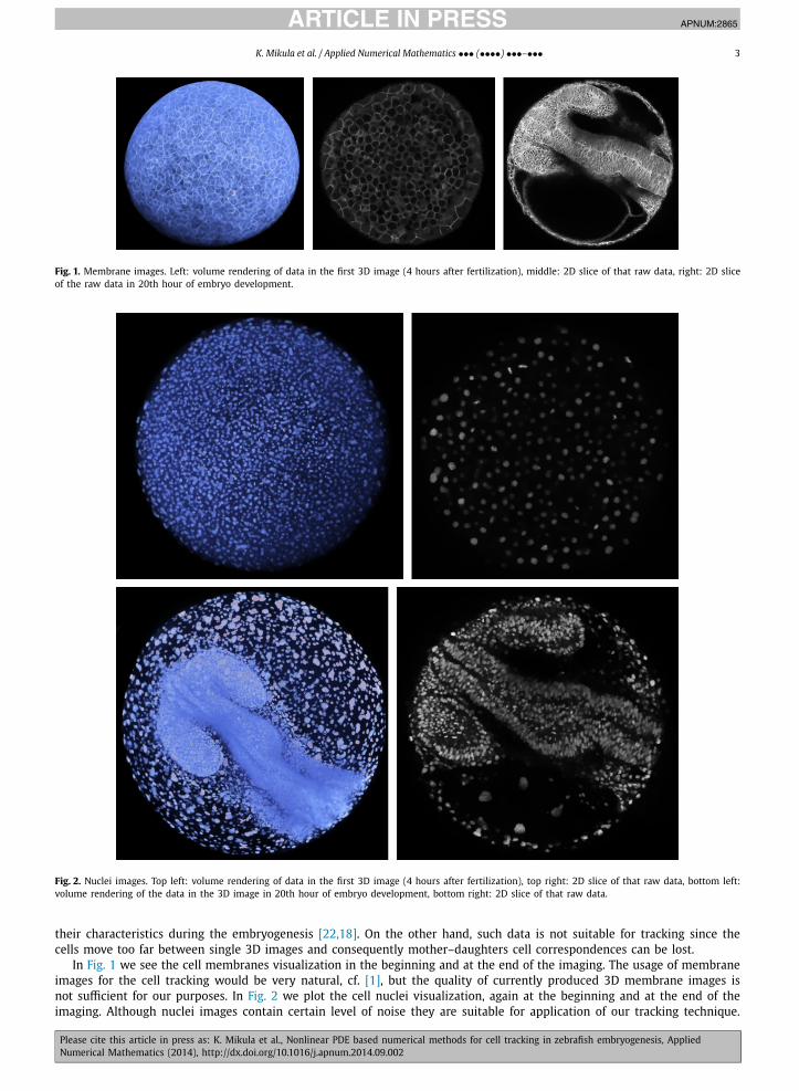
Fig. 1. Membrane images. Left: volume rendering of data in the first 3D image (4 hours after fertilization), middle: 2D slice of that raw data, right: 2D slice of the raw data in 20th hour of embryo development.

Fig. 2. Nuclei images. Top left: volume rendering of data in the first 3D image (4 hours after fertilization), top right: 2D slice of that raw data, bottom left: volume rendering of the data in the 3D image in 20th hour of embryo development, bottom right: 2D slice of that raw data.

their characteristics during the embryogenesis [22,18]. On the other hand, such data is not suitable for tracking since the cells move too far between single 3D images and consequently mother–daughters cell correspondences can be lost.

In Fig. 1 we see the cell membranes visualization in the beginning and at the end of the imaging. The usage of membrane images for the cell tracking would be very natural, cf. [1], but the quality of currently produced 3D membrane images is not sufficient for our purposes. In Fig. 2 we plot the cell nuclei visualization, again at the beginning and at the end of the imaging. Although nuclei images contain certain level of noise they are suitable for application of our tracking technique.



Fig. 3. Image filtering. Left: isosurface visualization of the original 3D data in 100th time step, right: the result after 10 filtering steps by GMCF.

In both figures we can observe how complex the development of organism in few first hours of embryogenesis is. It grows from an unorganized set of cells to various morphogenetic structures corresponding to future organs of the zebrafish adult.

For the testing of the method and for the extraction of cell trajectories we use the representative dataset with acquisition step dθ = 67 seconds, Nθ number of time steps and with dimension of every 3D image 512 × 512 × 104 voxels. The real voxel size is dx1 = dx2 = dx3 = 1.37 micrometer in every spatial dimension and the whole 3D+time sequence has 760 time steps. In this paper we present its processing up to time step Nθ = 479 in which the biologists selected manually cells forming presumptive organs during the zebrafish brain early embryogenesis. Using developed approach we can track those cell populations, see Section 5, and thus follow their dynamics and clonal history. Since the size of the single 3D image is about 27 MB, for 479 time steps we deal with about 13 GB of raw data which requires the usage of high-performance parallel computing facilities especially when designing spatially 4D numerical algorithms.

From a mathematical point of view, the 3D+time image sequence is understood as a function u(x1, x2, x3, θ), u : Λ →[0, 1], where Λ is a bounded spatio-temporal (rectangular) subdomain of R4. When we consider processing of 3D images, in Sections 2 and 3, we consider u at a corresponding time step θ , but for simplicity we denote it as u(x) = u(x1, x2, x3)

omitting the θ variable. Similarly, the subset of Λ for a given θ in 3D image processing will be denoted by Ω . Since our image processing algorithms are based on evolutionary PDEs we add the artificial time (filtering “time”, center detection “time”, “time” relaxation for the eikonal equation) variable t . This variable should not be confused with the real image sequence time θ .

2. Nonlinear diffusion filtering

The image filtering is the first step of our overall tracking procedure. The noise is intrinsically linked to the microscopy technique and its level increases with decreasing the time step dθ of the scanning. The careful study of various filtering methods was performed in [12] and the geodesic mean curvature flow (GMCF) was chosen as an optimal one with re-spect to smoothing of spurious noisy structures and sharpening the edges of 3D+time cell nuclei images during zebrafish embryogenesis. The GMCF filtering model is based on a discretization of the following nonlinear diffusion equation

ut − |∇u|∇.

(g(|∇Gσ ∗ u|) ∇u

|∇u|)

= 0, (1)

where u(t, x), t > 0, represents the filtered image intensity function. We start from the initial condition u(0, x) = u0(x), where u0 is an original 3D image and we consider few discrete time steps of the discretized model. We consider zero Neumann boundary conditions on the boundary ∂Ω of the 3D image domain Ω . In this model, the mean curvature motion of the level sets of function u is determined by the edge indicator function

g(s) = 1

1 + K s2, K ≥ 0 (2)

that is applied to the image gradient presmoothed by the Gaussian kernel Gσ with a small variance σ . The essential property of this function is that its negative gradient points towards the edges in the image and overall nonlinear diffusion process given by (1) causes accumulation of the level sets of u along the boundaries of objects in the image and therefore the filtering is also edge preserving. The filtered image uF is obtained as the solution of (1) at a time t = T F . The optimal choice of the model and discretization parameters was studied in [12] on the basis of the mean Hausdorff distance of the level sets of the filtered image and the manually segmented nucleus shapes. In Fig. 3 we present the filtering result by using optimal parameters of the GMCF model.

2.1. Discretization of the nonlinear diffusion filtering equation

For discretization of (1) in time we use the semi-implicit approach that guarantees unconditional stability of the numer-ical scheme. Let us suppose that we solve the PDE (1) in the interval [0, T F ] and let N F be a number of uniform time steps with size τF = T F /N F . The semi-implicit scheme for solving Eq. (1) is given by



un − un−1

τF− ∣∣∇un−1

∣∣∇.

(g(∣∣∇Gσ ∗ un−1

∣∣) ∇un

|∇un−1|)

= 0, (3)

where un represents the solution in the nth filtering step, n = 1 . . . N F .For spatial discretization of (3) we use the finite volume method. First, we identify the finite volumes of the mesh Th

with the voxels of the 3D image. We denote each finite volume by V ijk , i = 1 . . . N1, j = 1 . . . N2, k = 1 . . . N3. Such a finite volume grid is rectangular and let h1 = dx1, h2 = dx2, h3 = dx3 represent the size of the voxels in x1, x2, x3 direction, respectively. Let m(V ijk) denote the volume of V ijk and ci jk its barycenter. By un

ijk we denote the approximate value of un

in ci jk .For all volumes V ijk , we define two index sets. First, let Nijk denote the set of all (p, q, r) such that p, q, r ∈ {−1, 0, 1},

|p| + |q| + |r| = 1. Then, let Pijk represent the set of all (p, q, r) satisfying p, q, r ∈ {−1, 0, 1}, |p| + |q| + |r| = 2. Let us first consider (p, q, r) ∈ Nijk . The line connecting the center of V ijk and the center of its neighbor V i+p, j+q,k+r is denoted by bpqr

i jk and its length m(bpqri jk ). The faces of the finite volume V ijk are denoted by epqr

i jk with area m(epqri jk ) and normal ν pqr

i jk . Let xpqr

i jk be the point where the line bpqri jk crosses the face epqr

i jk . Finally, for any (p, q, r) ∈ Pijk , let ypqri jk denote the midpoints of

the voxel edges. The approximate value of un−1 at xpqri jk and ypqr

i jk , where (p, q, r) belongs to the corresponding index set, is denoted by upqr

i jk , omitting the time index, as only the values from the time level n − 1 will be needed in these points.

Now let us divide Eq. (3) by |∇un−1| and integrate it over every finite volume V ijk . After application of the Green theorem on the right hand side we get∫

V ijk

1

|∇un−1|un − un−1

τFdx =

∑Nijk

∫

epqri jk

g(∣∣∇Gσ ∗ un−1

∣∣) ∇un

|∇un−1|νpqri jk dγ . (4)

As one can see from Eq. (4) in order to proceed further we have to approximate |∇un−1| on voxel faces epqri jk and on voxel

V ijk itself. Similarly, the term g(|∇un−1σ |), un−1

σ = Gσ ∗un−1 must be approximated on the voxel faces. Moreover, the norm of the gradient |∇un−1| appears in denominator. Due to Evans and Spruck regularization approach [8], such term is substituted by the regularized one

√ε2 + |∇un−1|2, where ε is the regularization parameter, usually ε � 1. In order to approximate

(regularized) values of the gradient norm we define, cf. [14], values of un−1 in the midpoints ypqri jk of the voxel edges which

are approximated for any (p, q, r) ∈ Pijk by

upq0i jk = 1

4

(un−1

i jk + un−1i+p, j,k + un−1

i, j+q,k + un−1i+p, j+q,k

),

up0ri jk = 1

4

(un−1

i jk + un−1i+p, j,k + un−1

i, j,k+r + un−1i+p, j,k+r

),

u0qri jk = 1

4

(un−1

i jk + un−1i, j+q,k + un−1

i, j,k+r + un−1i, j+q,k+r

).

Let us denote by ∇ pqr un−1i jk the approximation of the gradient in the barycenter xpqr

i jk of the face epqri jk , (p, q, r) ∈ Nijk , of the

voxel V ijk . Using the above definitions, we can define gradient approximations on faces by

∇ p00un−1i jk = (

p(un−1

i+p, j,k − un−1i jk

)/h1,

(up10

i jk − up,−1,0i jk

)/h2,

(up01

i jk − up,0,−1i jk

)/h3

),

∇0q0un−1i jk = ((

u1q0i jk − u−1,q,0

i jk

)/h1,q

(un−1

i, j+q,k − un−1i jk

)/h2,

(u0q1

i jk − u0,q,−1i jk

)/h3

),

∇00run−1i jk = ((

u10ri jk − u−1,0,r

i jk

)/h1,

(u01r

i jk − u0,−1,ri jk

)/h2, r

(un−1

i, j,k+r − un−1i jk

)/h3

)and then the terms (including regularization) which we need in the scheme will be denoted by

Q pqr;n−1ε,i jk =

√ε2 + ∣∣∇ pqrun−1

i jk

∣∣2,

Q n−1ε,i jk =

√√√√ε2 + 1

6

∑Nijk

∣∣∇ pqrun−1i jk

∣∣2,

g pqr;n−1i jk = g

(∣∣∇ pqrun−1σ ;i jk

∣∣), (5)

where un−1σ ;i jk denotes the result of convolution of un−1 with Gaussian kernel in voxel V ijk . If we approximate the left hand

side of (4) by

∫V

1

|∇un−1|un − un−1

τFdx ≈ m(V ijk)

1

Q n−1ε,i jk

uni jk − un−1

i jk

τF·

i jk



Fig. 4. Cell center detection for the lth 3D image, l = 100. We plot a detail of the solution u(x1, x2, x3), x3 = 60h3 in the 0th (left), 10th (middle) and 30th (right) time step of LSCD evolution.

and using all further definitions in (5) we get discretization of (1) in the following form

m(V ijk)un

ijk − un−1i jk

τF= Q n−1

ε,i jk

∑Nijk

m(epqri jk )

m(bpqri jk )

g pqr;n−1i jk

Q pqr;n−1ε,i jk

(un

i+p, j+q,k+r − unijk

). (6)

The discrete equation (6), together with boundary conditions (the zero Neumann boundary conditions are treated by the reflection of inner values to additional finite volumes along the boundary) represent the linear system of equations with unknowns un

ijk , i = 1 . . . N1, j = 1 . . . N2, k = 1 . . . N3. The system is solved in each step n by the parallel Red–Black SOR iterative method implemented in the MPI framework. Since we start the iterative process using the result from the previous time step n −1, we have a good initial approximation and parallel SOR method is fast approaching the linear system solution.

3. Cell center detection

The second step of our approach is the detection of cell nuclei centers, we call them also cell identifiers. The cell center detection method is based on the fact that objects visible in the image can be seen as humps of relatively higher image intensity, bright nuclei on dark background is a typical example, see figures in Section 1.1. Any such hump is represented by certain image intensity level sets. The diameter of these level sets allows us to distinguish between significant objects, e.g. cell nuclei, and spurious inner structures which still remain after GMCF filtering. For cell nuclei, the diameter d is relatively large, 0 � c1 ≤ d ≤ c2, while the diameter of the spurious inner structures is much smaller, 0 < d � c1. If the level sets are moving (advected) at a constant speed in the direction of the inner normal, the encompassed volume is decreasing and finally the hump disappears. It is also well-known that if the evolution of the level set depends on its mean curvature (such evolution represents an intrinsic diffusion of the isosurfaces) then the speed of shrinking tends to infinity as the diameter of the level set tends to zero. So our model is based on the fact that the level sets with small diameter corresponding to spurious structures disappear quickly (by the above mentioned nonlinear advection–diffusion mechanism) while level sets representing cell nuclei are observable in a much longer time scale, in Fig. 4 we present example of such evolution computed by our model. Since the motion of every level set is given by the normal velocity V = δ + μk where δ and μ are constants (model parameters) and k is the mean curvature, we formulate our level set center detection (LSCD) method in the form of following nonlinear advection–diffusion equation [10]

ut + δ∇u

|∇u| .∇u − μ|∇u|∇.

( ∇u

|∇u|)

= 0 (7)

which is applied to the initial condition given by uF , the result of GMCF filtering. Again, we consider the zero Neumann boundary condition and the equation is solved in time interval [0, TC ]. Due to the shrinking and smoothing of all (real and spurious) structures in the evolutionary process represented by (7), we observe a decrease of the number of local maxima of the solution u as time proceeds. This decrease is fast in the beginning and much slower later and we stop this process when the speed of decrease is below a certain threshold. The cell centers are detected as points of local maxima of the function u at the stopping time TC . This is done for every 3D image of the sequence and usually 10 discrete time steps of LSCD model are sufficient to get high quality estimate of the cell identifiers. Moreover, if we still need to remove some false positives (more identifiers inside one nucleus) we can use the nucleus segmentation approach by generalized subjective surface (GSUBSURF) method [21,7,16,22] as described in [3], Section 6.3.1. The set of all cell identifiers detected in all time steps of the image sequence is denoted by sl

m , m = 1, . . . , nlC , l = 1, . . . , Nθ . In [3,22,18,4,13] the centers detected by LSCD

were used for various purposes including cell shape, epithelium and whole embryo segmentation and tracking.



Fig. 5. Examples of segmentation of cell nuclei using 3D GSUBSURF method [18].

3.1. Discretization of the nonlinear level set center detection equation

The time discretization of LSCD equation (7) is explicit in advective and semi-implicit in diffusion parts and it uses the finite volume method together with upwind principle for space discretization [9,10,14]. We chose a number of center detection steps NC and define a uniform time step size τC = TC /NC . Let us define integrated advective fluxes for (p, q, r) ∈Nijk by

v pqri jk = m

(epqr

i jk

)(δ

un−1i+p, j+q,k+r − un−1

i jk

Q pqr;n−1ε,i jk m(bpqr

i jk )

)(8)

and identify inflow boundaries by the index set Nini jk := {(p, q, r) ∈ Nijk, v

pqri jk ≤ 0}. Using these definitions and definitions (5)

we can write a discretization of Eq. (7) in the following form

m(V ijk)un

ijk − un−1i jk

τC=

∑Nin

i jk

v pqri jk

(un−1

i+p, j+q,k+r − un−1i jk

)

+ Q n−1ε,i jk

∑Nijk

m(epqr

i jk

)uni+p, j+q,k+r − un

ijk

Q pqr;n−1ε,i jk m(bpqr

i jk ). (9)

The method is parallelized in MPI framework and the Red–Black SOR parallel solver is used for solving the linear system (9)in every time step n.

4. Cell trajectories extraction and lineage tree construction

The main new idea of our cell tracking method is presented in this section. The tracking is based on the cell trajectories extraction which is done by finding centered paths inside a specifically constructed 4D spatio-temporal tree structure. The 4D spatio-temporal tree structure is a subset of all doxels (4 dimensional pixels) of the 3D image sequence which represents the 3D cell shapes moving (and splitting) in time. The method is composed by five basic steps:

• construction of a 4D segmentation yielding the 4D spatio-temporal tree structure,• computation of constrained 4D distance functions inside this 4D segmentation and designing of a proper combination

of them in order to build a potential field for tracking,• extraction of cell trajectories using the steepest descent direction of the potential field,• centering the extracted trajectories inside the 4D spatio-temporal trees in order to eliminate duplicates,• construction of the cell lineage tree by detecting trajectories which merge together when going backward in time

indicating mitosis and thus a branching node of the lineage tree.

4.1. 4D segmentation

We call 4D segmentation a spatio-temporal structure which approximates the space–time movement of nuclei in 3D+time image sequence. As one can see from Fig. 5 the shape of cell nuclei in 3D images is reasonably approximated by spheres or ellipsoids. Thus, in order to construct the 4D segmentation we use cell identifiers detected in all time steps,



Fig. 6. Projection of the 4D segmentation to one time step. For each cell identifier we can see central sphere (inside the red circle) surrounded by the overlaps from the previous time step (inside the green circle) and from the next time step (inside the blue circle). Three further parts of 4D segmentation are shown as well. (For interpretation of the references to color in this figure legend, the reader is referred to the web version of this article.)

slm , m = 1, . . . , nl

C , l = 1, . . . , Nθ , and create 4D ellipsoids around all these points. Currently we are using the same halfaxes in space equal to 2dx, where dx = dy = dz is voxel size (same in all three spatial dimensions) and with halfaxis equal to dθ

in temporal dimension. The nonzero temporal halfaxis is important due to the time overlap which we create and thus we achieve better connectivity of 4D spatio-temporal tree structures, Fig. 6 shows our 4D segmentation projected to one time step. Thanks to the time overlap we also make connected such branches of the 4D spatio-temporal tree where a cell center is not detected in one frame but it is detected in two neighboring frames and thus we correct false negative errors of the cell center detection algorithm.

We also have to note that our current approach is not optimal in the sense of getting real 4D image segmentation of cell nuclei movement. Such approach using 4D generalized subjective surface (GSUBSURF) method was originally developed in [17] but used only locally in time (for short time sequence) and space (for a detail of the full 3D volume) and utilization of such type of method for long 3D+time image sequences remains a great challenge from modeling, discretization and (parallel) computation point of view and it will be objective of our further study. On the other hand, the simplified approach suggested and used in this paper also gives, thanks to the time overlap, the reliable 4D segmentation which can be used in further steps of cell trajectories extraction.

4.2. Constrained distance functions

Our 4D segmentation containing 4D spatio-temporal tree structures can be represented by a 4D piecewise constant function, with some BIG value outside of the segmentation and with zero value inside it. Using this information, we compute two types of distance functions inside the 4D spatio-temporal tree structures. We call them constrained because all the calculations are constrained by the boundaries of the 4D segmentation. Due to that fact, the computed distances between 4D points of the 3D+time image sequence are not a standard Euclidean distances in R4 but they represent a minimal Euclidean paths between the points inside the 4D segmentation.

The first type of distance functions will be denoted by Dl(x1, x2, x3, θ), l ≥ 1. The function Dl(x1, x2, x3, θ) represents the distance of any inner point (x1, x2, x3, θ) of the 4D segmentation to the set of cell identifiers {sl

m, m = 1, . . . , nlC } detected

in the lth time step. Moreover we impose the constraints that Dl(x1, x2, x3, θ) = BIG if θ < l, which means we look only forward in time when computing Dl , and Dl(x1, x2, x3, θ) = BIG for all (x1, x2, x3, θ) outside of the 4D segmentation. It is worth to note that we compute Dl for all time steps l = 1, . . . , Nθ of the image sequence so it represents the most computationally demanding part of our approach. The second type of distance function, D B (x1, x2, x3, θ), is computed just once and it represents the distance of any inner point of the 4D segmentation to the boundary of the 4D segmentation. In this case, D B(x1, x2, x3, θ) = 0 for all (x1, x2, x3, θ) outside of the 4D segmentation. Both types of distance functions are computed numerically on the doxel structure of the 3D+time image sequence using the 4D Rouy–Tourin scheme. The scheme is presented in the next section.

Together with computing constrained distance functions Dl(x1, x2, x3, θ), l ≥ 1, we subsequently build their combination denoted by D(x1, x2, x3, θ). The combined distance function D(x1, x2, x3, θ) is built in such a way that it gives the max-imal shortest distance of a point (x1, x2, x3, θ) of the 4D segmentation to a cell identifier sl

m among all m and all l ≤ θ . Simply saying, it represents the distance to the most far cell identifier to which the point (x1, x2, x3, θ) is continuouslyconnected inside the 4D segmentation. Such construction of the combined distance function D will help us to get all, also partial, cell trajectories contained in our 4D spatio-temporal tree structures. Its utilization represents a main important novelty with respect to [1,17] where just D = D1 was used so only cell trajectories starting in the first frame could be detected.



Fig. 7. On the left we can see the plot of the constrained distance function D1, in the middle we can see the plot of the constrained distance function Dl , l > 1 and on the right we can see the plot of the combined distance function D after time step l. Information about the (most left) simply connected component of the 4D segmentation which was not detected in the 1st time step is added into the function D in time step l. The values of D in the previously detected simply connected components were not changed by values of Dl .

Fig. 8. On the left we can see the plot of values for a constrained distance function Dl in one simply connected component of the 4D segmentation, on the right we can see the plot of values for the constrained distance function D B in the same simply connected component. (For interpretation of the references to color in this figure, the reader is referred to the web version of this article.)

In order to construct the combined distance function D , first we define a set of values

D(x1, x2, x3, θ) = {Dl(x1, x2, x3, θ); l ∈ {1,2, . . .}, Dl(x1, x2, x3, θ) < BIG

}and then we set

D(x1, x2, x3, θ) ={

maxD(x1, x2, x3, θ), D(x1, x2, x3, θ) = ∅BIG otherwise.

In Fig. 7 we show how the combined distance function contains information about all simply connected components of the 4D segmentation. Inside the valleys encompassed by the BIG values, the value of D is growing from zero, in cell identifier where any simply connected component begins, up to a maximal value, where the simply connected component ends.

Now, looking at Fig. 7 and also Fig. 8 left, we can think about D as a potential field and traverse it in the steepest descent direction from the highest value in every simply connected component to the zero value. The paths obtained in such way would represent good approximation of the space–time cell trajectories. And, if the 4D segmentation would contain only perfectly separated 4D spatio-temporal tree structures, we would obtain correctly all (also partial) cell trajectories which can be extracted from the data. Unfortunately, in the real 4D data it is not always the case and we must deal with imperfections given mainly by a cells overlapping. In order to overcome this difficulty we have to keep the extracted paths at a certain distance from the spatio-temporal cell boundaries or, in other words, they should be more centered inside the 4D segmentation. This can be achieved by using the constrained distance function D B (x1, x2, x3, θ) [15,1,17] values of which grow from boundaries to the center of the 4D spatio-temporal trees, see Fig. 8 right. Based on these facts we build the new potential field

V (x1, x2, x3, θ) = D(x1, x2, x3, θ) − D B(x1, x2, x3, θ) (10)

which will be used in our algorithm for the extraction of cell trajectories.



4.3. Numerical method for computing the constrained distance function

For the calculation of the constrained distance functions we solve numerically the so-called time relaxed eikonal equation

dt + |∇d| = 1 (11)

for the unknown function d(x1, x2, x3, θ, t). In contrast to Sections 2 and 3 we solve here spatially 4D problem, so ∇dis a 4D gradient of the function d, i.e. the vector of partial derivatives with respect to x1, x2, x3 and θ variables. For the discretization of Eq. (11) we use spatially the 4D Rouy–Tourin scheme [20]. The constrained distance function, which we look for, is obtained as an equilibrium of the numerical solution, i.e. it satisfies numerically the classical eikonal equation |∇d| = 1. When solving Eq. (11), the values of the solution at points outside the 4D segmentation are fixed to a BIG value which is arbitrary but bigger than any distance which can be obtained for points inside the 4D segmentation. For Eq. (11), we have to prescribe zero Dirichlet condition on the set from which we compute the distances. In case of computing the constrained distance function Dl we prescribe the zero values to the set of cell identifiers {sl

m, m = 1, . . . , nlC } detected in

the lth time step. In case of computing the constrained distance function D B we prescribe the zero values for all boundary points of the 4D segmentation.

In analogy with Sections 2 and 3, where we solve spatially 3D problems, we identify here the 4D doxels with finite volumes V ijkl having four indices. Without losing generality, we rescale the time step dθ to be equal to dx1 = dx2 = dx3and denote their common value by hD (standardly we set hD = 1). Let dn

ijkl denote the approximate value of solution d in barycenter of V ijkl in a discrete step tn = nτD where τD is the length of step discretizing t variable. Then, for every V ijklwe define the index set Nijkl of all (p, q, r, s) such that p, q, r, s ∈ {−1, 0, 1}, |p| + |q| + |r| + |s| = 1. In order to build the scheme, for any (p, q, r, s) ∈ Nijkl , we define (see formula (10) in [20])

D pqrsi jkl = (

min(dn−1

i+p, j+q,k+r,l+s − dn−1i jkl ,0

))2(12)

and then also

M1000i jkl = max

(D−1,0,0,0

i jkl , D1,0,0,0i jkl

), M0100

i jkl = max(

D0,−1,0,0i jkl , D0,1,0,0

i jk

)M0010

i jkl = max(

D0,0,−1,0i jkl , D0,0,1,0

i jkl

), M0001

i jkl = max(

D0,0,0,−1i jkl , D0,0,0,1

i jkl

). (13)

Using these notations, the 4D Rouy–Tourin scheme for solving Eq. (11) has the following form

dnijkl = dn−1

i jkl + τD − τD

hD

√M1000

i jkl + M0100i jkl + M0010

i jkl + M0001i jkl . (14)

Due to stability reasons, the coupling τD = hD/2 is used. We also speed-up the basic algorithm (14) by subsequently omitting calculations in points which are already in equilibrium using the fixing strategy proposed in [2], see also [18].

The method (14) with the fixing was parallelized using OpenMP programming interface for shared memory parallel servers. Such parallel implementation can be used for processing the long-time image sequences, e.g. the one with 479 3D volumes discussed in Section 5. In that case we needed almost 200 GB of shared memory and we obtained the speed-up 23.5 for 32 threads. Such speed-up was obtained thanks to the utilization of the NUMA library functions which allow the optimal NUMA nodes memory usage on the nowadays standard servers with NUMA (non-uniform memory access) architecture.

4.4. Extraction of the cell trajectories

The cell trajectory is represented by a series of points in space–time (discrete spatio-temporal curve) for which we prescribe the condition that there exists exactly one point Pl of the trajectory in time step l = Nb, . . . , Ne , 1 ≤ Nb < Ne ≤ Nθ . The extraction of cell trajectories is realized in two steps:

• first, we use backtracking in time by the steepest descent direction of the potential V built in (10) starting from all cell identifiers sl

m , m = 1, . . . , nlC detected in all time steps l = 2, . . . , Nθ ,

• then, we center all the extracted trajectories inside the 4D spatio-temporal trees, by using the constrained distance function D B , in order to eliminate duplicates.

The first step is realized as follows: Let sem be one of the cell centers detected in the eth time step. We search recursively in

the nearest vicinity of sem , but only in the current time step e and the previous time step e − 1, for a doxel with the minimal

value of the potential V strictly less than its value at sem . The cell trajectory point P e for the time step e is defined as the

(last in search) doxel from which we move to a point in the previous time step e − 1. Then from this point we continue the same search, etc. We end the process when we cannot move from the time step b to the previous time step b − 1 by decreasing the value of potential V . Then the last point of the search in time step b, which must be some detected center, becomes the first point of the cell trajectory starting in the time step b and ending in time step e (when going forward in



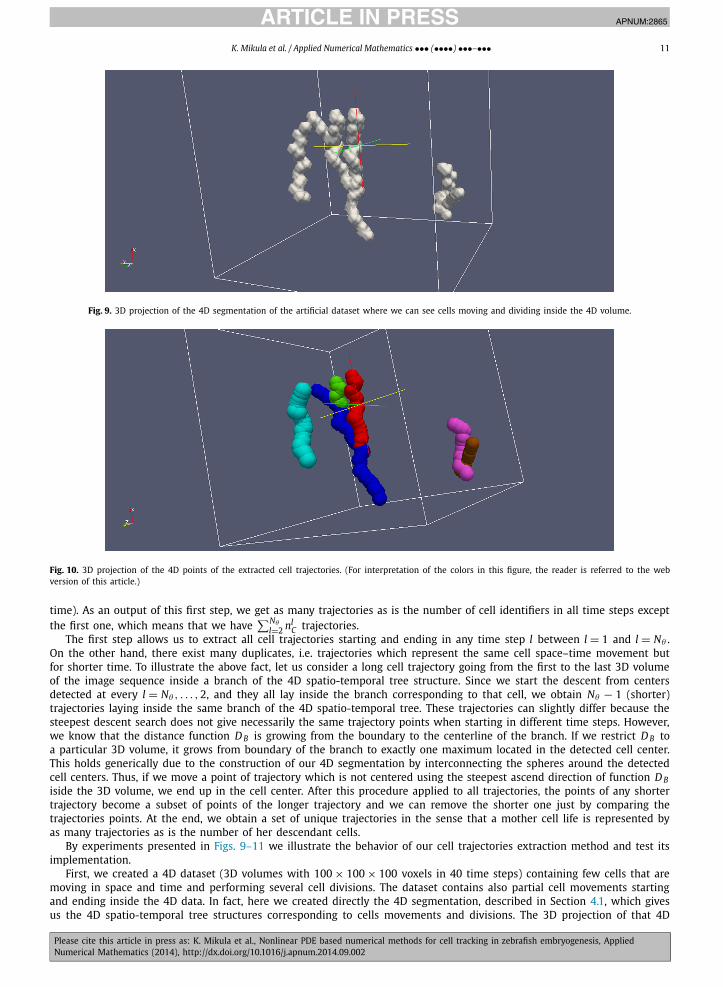
Fig. 9. 3D projection of the 4D segmentation of the artificial dataset where we can see cells moving and dividing inside the 4D volume.

Fig. 10. 3D projection of the 4D points of the extracted cell trajectories. (For interpretation of the colors in this figure, the reader is referred to the web version of this article.)

time). As an output of this first step, we get as many trajectories as is the number of cell identifiers in all time steps except the first one, which means that we have

∑Nθ

l=2 nlC trajectories.

The first step allows us to extract all cell trajectories starting and ending in any time step l between l = 1 and l = Nθ . On the other hand, there exist many duplicates, i.e. trajectories which represent the same cell space–time movement but for shorter time. To illustrate the above fact, let us consider a long cell trajectory going from the first to the last 3D volume of the image sequence inside a branch of the 4D spatio-temporal tree structure. Since we start the descent from centers detected at every l = Nθ , . . . , 2, and they all lay inside the branch corresponding to that cell, we obtain Nθ − 1 (shorter) trajectories laying inside the same branch of the 4D spatio-temporal tree. These trajectories can slightly differ because the steepest descent search does not give necessarily the same trajectory points when starting in different time steps. However, we know that the distance function D B is growing from the boundary to the centerline of the branch. If we restrict D B to a particular 3D volume, it grows from boundary of the branch to exactly one maximum located in the detected cell center. This holds generically due to the construction of our 4D segmentation by interconnecting the spheres around the detected cell centers. Thus, if we move a point of trajectory which is not centered using the steepest ascend direction of function D Biside the 3D volume, we end up in the cell center. After this procedure applied to all trajectories, the points of any shorter trajectory become a subset of points of the longer trajectory and we can remove the shorter one just by comparing the trajectories points. At the end, we obtain a set of unique trajectories in the sense that a mother cell life is represented by as many trajectories as is the number of her descendant cells.

By experiments presented in Figs. 9–11 we illustrate the behavior of our cell trajectories extraction method and test its implementation.

First, we created a 4D dataset (3D volumes with 100 × 100 × 100 voxels in 40 time steps) containing few cells that are moving in space and time and performing several cell divisions. The dataset contains also partial cell movements starting and ending inside the 4D data. In fact, here we created directly the 4D segmentation, described in Section 4.1, which gives us the 4D spatio-temporal tree structures corresponding to cells movements and divisions. The 3D projection of that 4D



Fig. 11. Separated trajectories after tracking, before post processing centering.

Fig. 12. A detail of the extracted cell lineage tree.

segmentation is given in Fig. 9. Then we performed computations of constrained distance functions Dl , l = 1, . . . , 40 together with building of the combined distance function D and computation of the constrained distance function D B . After, we built the potential V and performed both steps (the steepest descent of V and centering by D B ) of cell trajectories extraction. The resulting extracted trajectories are presented in Fig. 10. By different colors we plot 3D projection of 4D points (represented by small 4D spheres) of different trajectories. As we can see, all trajectories, including partial and dividing, are correctly extracted. Since the trajectories are overlapping we can see only the color of the last drawn one, e.g. the red trajectory is the same as the blue one before the first division.

In the second testing example, we created two touching branches of a 4D segmentation imitating situation that the cell nuclei are not perfectly separated due to acquisition errors. And, we tested our method in an extremal case when the branches are fully overlapped in space in two subsequent time steps (we used the same cell identifiers for those two time steps when building the 4D segmentation). In Fig. 11 we present the result obtained after the first step of our method, i.e. after the backtracking in time by the steepest descent direction of V . Since we perform only the steepest descent and not the centering in this step, we can obtain two separated paths. When we center them in the second step they will remain different (although with two equal points) and thus they will represent two correctly extracted cell trajectories.

4.5. Cell lineage tree reconstruction

Let us consider a mother cell which is going to divide at time step l, i.e. at time step l + 1 it has two descendants and in later times maybe more due to further divisions. Without losing generality, let the number of descendant of this cell in the whole image sequence be Nd = 2m . As noticed already in the previous section, up to time l the life of the cell is represented by exactly Nd trajectories which are, however, until time l composed by the same spatio-temporal points. From the time l + 1, the half of trajectories differs from the second half, but every half is again composed by the same points until the next division. The representation of cell life by the multiple trajectories which are partially the same does not cause any problem in visualization and/or reconstruction of single cell or cell population movements and divisions. However, the reduction of the equal multiple parts of trajectories is necessary for the reconstruction of the cell lineage tree and is explained below.



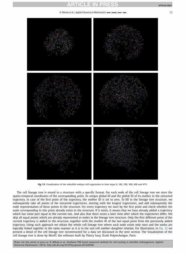
Fig. 13. Visualization of the zebrafish embryo cell trajectories in time steps 0, 100, 200, 300, 400 and 479.

The cell lineage tree is stored in a structure with a specific format. For each node of the cell lineage tree we store the spatio-temporal coordinates of the corresponding point, its unique global ID and the global ID of its mother in the extracted trajectory. In case of the first point of the trajectory, the mother ID is set to zero. To fill in the lineage tree structure, we subsequently take all points of the extracted trajectories, starting with the longest trajectories, and add subsequently the node representation of those points to the structure. For every trajectory we start by the first point and check whether the node corresponding to this point already exists in the structure. If it exists, it means that we have already added a trajectory which has some part equal to the current one. And also that there exists a later time after which the trajectories differ. We skip all equal points which are already represented as nodes in the lineage tree structure. Only the first different point of the current trajectory is added to the structure, together with the mother ID of the last equal point from the previously added trajectory. Using such approach we obtain the whole cell lineage tree where each node exists only once and the nodes are logically linked together in the same manner as it is in the real cell mother–daughter relation. For illustration, in Fig. 12 we present a detail of the cell lineage tree reconstructed for a data set discussed in the next section. The visualization of the cell lineage tree is done by MovIT, the software built by Thiery Savy, École Polytechnique, Paris.



Fig. 14. Visualization of the formation of presumptive organs during embryogenesis obtained by backward tracking of cells selected by biologists in time step 479. The visualization presents seven cell populations in time steps 0, 100, 200, 300, 400 and 479. (For interpretation of the colors in this figure, the reader is referred to the web version of this article.)

5. Numerical experiment on real zebrafish embryogenesis data

We performed the cell tracking by the approach designed in Sections 2–4 on the dataset described in Section 1.1representing the zebrafish brain early embryogenesis. All 3D images were filtered by 10 steps of GMCF model and the cell nuclei identifiers were detected by 10 steps of LSCD algorithm. From several millions of cell identifiers we built the 4D segmentation and then the cell trajectories were extracted by the approach developed in Section 4. We present here Figs. 13–16 showing results of the tracking procedure. In Fig. 13 one can see the visualization of the



Fig. 15. The cell population movement visualized by long parts of trajectories. Top left: trajectories from time step 0 to time step 120, top right: from 120 to 240, bottom left: from 240 to 360, bottom right: from 360 to 479.

cell trajectories in developing embryo. To that goal we built software, running on graphics card, where we can fluently zoom, rotate and animate in time a 3D scene even with a very high number of trajectories. The trajectories are dis-played as short lines (in random colors) connecting few subsequent spatio-temporal points with a freely chosen starting time.

In Fig. 14 we use a similar visualization, but we show trajectories only for a subset of all cells and different colors represent different cell populations trajectories. The subset represents seven cell populations forming different presumptive organs in the zebrafish embryo brain, e.g. hypoblast including pre-chordal-plate and notochord (red), presumptive hypotha-lamus (yellow), ventral telencephalon (brown), right eye (blue) or left eye (green). By the colored ellipsoid we also plot a motion of the mean trajectory of every cell population. One can see the evolution of cells from the 0th still chaotic stage, through 100th, 200th, 300th, 400th time steps where the cells are becoming more compactly localized up to 479th time step where the cells were marked by biologists. In order to have more dynamical impression, in Fig. 14 we show long parts of cell trajectories to illustrate the cell population movements from the central part up to the presumptive organ stage.

The last series of plots, in Fig. 16, presents the tracking of a single cell in several subsequent time steps of embryogenesis. One can see that the cell moves in a complicated manner, however, the visual inspection in 3D+time data shows that its trajectory is correct.

At the end of this section we shortly discuss an important difference between our new approach and previously sug-gested approaches [1,17]. In [1,17], only the distance function D1 was used instead of combined distance function D . It means that we can extract only cell trajectories laying in simply connected components of 4D segmentation starting in the first time step of the image sequence. After the centering step such trajectories are composed by a subset of all detected cell centers. For real data experiment presented in this section, such extracted trajectories would cover only 52% of all cell centers, which means we would lose many partial cell trajectories which can be extracted from the data by the new ap-proach. In fact, by using the method presented in this paper, the extracted cell trajectories cover all detected cell centers, which is an important improvement obtained by using the combined distance function D .

6. Conclusions

In this paper we developed a new approach to the cell tracking in 3D+time confocal microscopy data. We applied the tracking method to complex stages of the zebrafish early embryogenesis images. Together with [13] it is a first cell tracking



Fig. 16. Tracking of a single cell (green cross) displayed together with 2D slice of 3D data where the current cell identifier is localized. The visualization is presented for time steps 0, 100, 200 and 300. On the left: the 2D slice of current cell location, on the right: detail of the 2D slice with tracked cell better visible. (For interpretation of the references to color in this figure legend, the reader is referred to the web version of this article.)



method able to deal with such type of data. We discussed mathematical models in form of nonlinear PDEs the tracking method is based on and we also present their numerical discretizations which leads to parallel computing algorithms.

Acknowledgement

We thank to all former members of EC Embryomics and BioEmergences project teams, particularly to Paul Bourgine whose continuous encouragement has helped to obtain presented results.

References

[1] Y. Bellaïche, F. Bosveld, F. Graner, K. Mikula, M. Remešíková, M. Smíšek, New robust algorithm for tracking cells in videos of drosophila morphogenesis based on finding an ideal path in segmented spatio-temporal cellular structures, in: Proceeding of the 33rd Annual International IEEE EMBS Conference, Boston Marriott Copley Place, Boston, MA, USA, August 30–September 3, 2011, IEEE Press, 2011.

[2] P. Bourgine, P. Frolkovic, K. Mikula, N. Peyriéras, M. Remešíková, Extraction of the intercellular skeleton from 2D microscope images of early embryo-genesis, in: Proceeding of the 2nd International Conference on Scale Space and Variational Methods in Computer Vision, Voss, Norway, June 1–5, 2009, in: Lecture Notes in Computer Science, vol. 5567, Springer, 2009, pp. 38–49.

[3] P. Bourgine, R. Cunderlík, O. Drblíková, K. Mikula, N. Peyriéras, M. Remešíková, B. Rizzi, A. Sarti, 4D embryogenesis image analysis using PDE methods of image processing, Kybernetika 46 (2) (2010) 226–259.

[4] M. Campana, B. Maury, M. Dutreix, N. Peyriéras, A. Sarti, Methods toward in vivo measurement of zebrafish epithelial and deep cell proliferation, Comput. Methods Programs Biomed. 98 (2) (2010) 103–117.

[5] V. Caselles, R. Kimmel, G. Sapiro, Geodesic active contours, Int. J. Comput. Vis. 22 (1997) 67–79.[6] Y. Chen, B.C. Vemuri, L. Wang, Image denoising and segmentation via nonlinear diffusion, Comput. Math. Appl. 39 (5–6) (2000) 131–149.[7] S. Corsaro, K. Mikula, A. Sarti, F. Sgallari, Semi-implicit co-volume method in 3D image segmentation, SIAM J. Sci. Comput. 28 (6) (2006) 2248–2265.[8] L.C. Evans, J. Spruck, Motion of level sets by mean curvature, J. Differ. Geom. 33 (1991) 635–681.[9] P. Frolkovic, K. Mikula, Flux-based level set method: a finite volume method for evolving interfaces, Appl. Numer. Math. 57 (4) (2007) 436–454.

[10] P. Frolkovic, K. Mikula, N. Peyriéras, A. Sarti, A counting number of cells and cell segmentation using advection-diffusion equations, Kybernetika 43 (6) (2007) 817–829.

[11] S. Kichenassamy, A. Kumar, P. Olver, A. Tannenbaum, A. Yezzi, Conformal curvature flows: from phase transitions to active vision, Arch. Ration. Mech. Anal. 134 (1996) 275–301.

[12] Z. Krivá, K. Mikula, N. Peyriéras, B. Rizzi, A. Sarti, O. Stašová, 3D early embryogenesis image filtering by nonlinear partial differential equations, Med. Image Anal. 14 (4) (2010) 510–526.

[13] C. Melani, Algoritmos de procesamiento de imagenes para la reconstruccion del desarrollo embrionario del pez cebra. Computer Science PhD Thesis, UBA, FCEN, Buenos Aires, Argentina, 2013.

[14] K. Mikula, M. Remešíková, Finite volume schemes for the generalized subjective surface equation in image segmentation, Kybernetika 45 (4) (2009) 646–656.

[15] K. Mikula, J. Urbán, 3D curve evolution algorithm with tangential redistribution for a fully automatic finding of an ideal camera path in virtual colonoscopy, in: Proceedings of the Third International Conference on Scale Space Methods and Variational Methods in Computer Vision, Ein Gedi, Israel, 2011, in: Lecture Notes in Computer Science, vol. 6667, 2012, pp. 640–652.

[16] K. Mikula, N. Peyriéras, M. Remešíková, A. Sarti, 3D embryogenesis image segmentation by the generalized subjective surface method using the finite volume technique, in: Proceedings of FVCA5–5th International Symposium on Finite Volumes for Complex Applications, ISTE and WILEY, London, 2008, pp. 585–592.

[17] K. Mikula, N. Peyriéras, M. Remešíková, M. Smíšek, 4D numerical schemes for cell image segmentation and tracking, in: J. Fort, et al. (Eds.), Finite Volumes in Complex Applications VI, Problems & Perspectives, Proceedings of the Sixth International Conference on Finite Volumes in Complex Appli-cations, Prague, June 6–10, 2011, Springer Verlag, 2011, pp. 693–702.

[18] K. Mikula, N. Peyriéras, M. Remešíková, O. Stašová, Segmentation of 3D cell membrane images by PDE methods and its applications, Comput. Biol. Med. 41 (6) (2011) 326–339.

[19] R. Mikut, T. Dickmeis, W. Driever, P. Geurts, F.A. Hamprecht, B.X. Kausler, M.J. Ledesma-Carbayo, R. Marée, K. Mikula, P. Pantazis, O. Ronneberger, A. Santos, R. Stotzka, U. Strähle, N. Peyriéras, Automated processing of zebrafish imaging data: a survey, Zebrafish (2013), http://dx.doi.org/10.1089/zeb.2013.0886.

[20] E. Rouy, A. Tourin, Viscosity solutions approach to shape-from-shading, SIAM J. Numer. Anal. 29 (3) (1992) 867–884.[21] A. Sarti, R. Malladi, J.A. Sethian, Subjective surfaces: a method for completing missing boundaries, Proc. Natl. Acad. Sci. USA 12 (97) (2000) 6258–6263.[22] C. Zanella, M. Campana, B. Rizzi, C. Melani, G. Sanguinetti, P. Bourgine, K. Mikula, N. Peyrieras, A. Sarti, Cells segmentation from 3-D confocal images

of early zebrafish embryogenesis, IEEE Trans. Image Process. 19 (3) (2010) 770–781.

http://refhub.elsevier.com/S0168-9274(14)00154-8/bib626F73746F6Es1



http://refhub.elsevier.com/S0168-9274(14)00154-8/bib6E6F72776179s1



http://refhub.elsevier.com/S0168-9274(14)00154-8/bib6B796232303130s1


http://refhub.elsevier.com/S0168-9274(14)00154-8/bib6D617474656Fs1

http://refhub.elsevier.com/S0168-9274(14)00154-8/bib6D617474656Fs1


http://refhub.elsevier.com/S0168-9274(14)00154-8/bib76656D757269s1


http://refhub.elsevier.com/S0168-9274(14)00154-8/bib6573s1




http://refhub.elsevier.com/S0168-9274(14)00154-8/bib6B6B6F7479s1

http://refhub.elsevier.com/S0168-9274(14)00154-8/bib6B6B6F7479s1

http://refhub.elsevier.com/S0168-9274(14)00154-8/bib6B6D707273s1

http://refhub.elsevier.com/S0168-9274(14)00154-8/bib6B6D707273s1

http://refhub.elsevier.com/S0168-9274(14)00154-8/bib43616D696C6F546865736973s1

http://refhub.elsevier.com/S0168-9274(14)00154-8/bib43616D696C6F546865736973s1



http://refhub.elsevier.com/S0168-9274(14)00154-8/bib4D55636F6C6F6E6Fs1









http://refhub.elsevier.com/S0168-9274(14)00154-8/bib63626Ds1

http://refhub.elsevier.com/S0168-9274(14)00154-8/bib63626Ds1

http://dx.doi.org/10.1089/zeb.2013.0886



http://refhub.elsevier.com/S0168-9274(14)00154-8/bib7A616E656C6C61s1

http://refhub.elsevier.com/S0168-9274(14)00154-8/bib7A616E656C6C61s1

http://dx.doi.org/10.1089/zeb.2013.0886

Applied Numerical Mathematics - LIRMM

Documents

Transcript of Applied Numerical Mathematics - LIRMM