Applied Mathematics - GitHub Pagessethc23.github.io/wiki/Python/good_python_intro.pdfto other topics...

Applied Mathematics

and

Computing

Volume I

List of Contributors

J. HumpherysBrigham Young University

J. WebbBrigham Young University

R. MurrayBrigham Young University

J. WestUniversity of Michigan

R. GroutBrigham Young University

K. FinlinsonBrigham Young University

A. Zaitze↵Brigham Young University

i

ii List of Contributors

Preface

This lab manual is designed to accompany the textbook Foundations of Ap-plied Mathematics by Dr. J. Humpherys.

cThis work is licensed under the Creative Commons Attribution 3.0 UnitedStates License. You may copy, distribute, and display this copyrighted work only ifyou give credit to Dr. J. Humpherys. All derivative works must include an attribu-tion to Dr. J. Humpherys as the owner of this work as well as the web address to

https://github.com/ayr0/numerical_computing

as the original source of this work.To view a copy of the Creative Commons Attribution 3.0 License, visit

http://creativecommons.org/licenses/by/3.0/us/

or send a letter to Creative Commons, 171 Second Street, Suite 300, San Francisco,California, 94105, USA.

iii

https://github.com/ayr0/numerical_computing

http://creativecommons.org/licenses/by/3.0/us/

5/2/13 IPython Notebook

127.0.0.1:8888/7344a512-2932-4022-8f67-260318011223/print 1/13

Introduction to Python

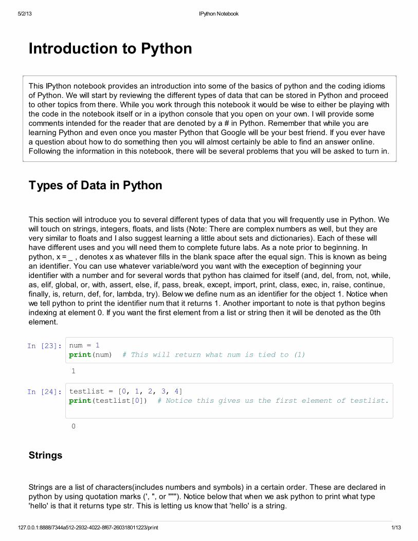
This IPython notebook provides an introduction into some of the basics of python and the coding idioms

of Python. We will start by reviewing the different types of data that can be stored in Python and proceed

to other topics from there. While you work through this notebook it would be wise to either be playing with

the code in the notebook itself or in a ipython console that you open on your own. I will provide some

comments intended for the reader that are denoted by a # in Python. Remember that while you are

learning Python and even once you master Python that Google will be your best friend. If you ever have

a question about how to do something then you will almost certainly be able to find an answer online.

Following the information in this notebook, there will be several problems that you will be asked to turn in.

Types of Data in Python

This section will introduce you to several different types of data that you will frequently use in Python. We

will touch on strings, integers, floats, and lists (Note: There are complex numbers as well, but they are

very similar to floats and I also suggest learning a little about sets and dictionaries). Each of these will

have different uses and you will need them to complete future labs. As a note prior to beginning. In

python, x = _ , denotes x as whatever fills in the blank space after the equal sign. This is known as beingan identifier. You can use whatever variable/word you want with the exeception of beginning your

identifier with a number and for several words that python has claimed for itself (and, del, from, not, while,

as, elif, global, or, with, assert, else, if, pass, break, except, import, print, class, exec, in, raise, continue,

finally, is, return, def, for, lambda, try). Below we define num as an identifier for the object 1. Notice when

we tell python to print the identifier num that it returns 1. Another important to note is that python begins

indexing at element 0. If you want the first element from a list or string then it will be denoted as the 0th

element.

In [23]:

In [24]:

Strings

Strings are a list of characters(includes numbers and symbols) in a certain order. These are declared in

python by using quotation marks (', ", or """). Notice below that when we ask python to print what type

'hello' is that it returns type str. This is letting us know that 'hello' is a string.

num = 1print(num) # This will return what num is tied to (1)

1

testlist = [0, 1, 2, 3, 4]print(testlist[0]) # Notice this gives us the first element of testlist.

0


127.0.0.1:8888/7344a512-2932-4022-8f67-260318011223/print 2/13

In [3]:

There are several operations that can be done to strings. Typically strings are useful for printing updates

or information from the code, but they can be used for other things as well (such as creating urls to direct

python to). For example, when printing, you can print multiple lines within one print statement by using \n.

You can also concatenate(add). Look at the difference between the examples below.

In [27]:

In [29]:

We can also slice(pull specific elements from) strings. Look at the examples below (The %s is a place

holder for what comes after %) :

In [36]:

We can also access a range of elements from strings in the following way.

In [39]:

Now see what the command [::-1] does after the string.

In [41]:

print(type('hello'))'hello'

<type 'str'>

Out[3]: 'hello'

str1 = 'welcome'str2 = 'to'str3 = 'bootcamp'print(str1 + str2 + str3) # Here we just print the strings concatenated together

welcometobootcamp

print(str1 + ' \n'+str2 + ' \n'+str3)# Here we concatenate&printthe strings and add \n

welcome to bootcamp

practicestr = 'abcdefghi'print('first element of practicestr is "%s"' % practicestr[0])

first element of practicestr is "a"

pracstr = 'abcdefghi'print(pracstr[0:]) # The : means everything afterwards. This will print whole string.print(pracstr[5:]) # This will print from element 5 on

abcdefghifghi

pracstr = 'abcdefghi'# Write your practice command here


127.0.0.1:8888/7344a512-2932-4022-8f67-260318011223/print 3/13

There are other things that you can do with strings, but this should suffice for now. A couple of the other

cool things are included below (The actual command is after the %). If you want more instruction on any

of these, ask questions.

In [73]:

Integers and Floats

Integers are exactly what they sound like. Integers are all positive and negative integers;; for you math

folk it is . Floats are all of the real numbers, . It is important to note the difference in programming

between integers and floats because their operations will do different things. To declare a number as a

float, you either need to tell the computer it is a float via command or add a decimal place. See below:

In [46]:

In [45]:

In [47]:

In [63]:

In [64]:

string = 'thisisasentencestring'capitallets = 'ABCDEFGH'print('number of a\'s in string = %s') %string.count('a')print('string in all upper case is %s') %string.upper()print('capitallets in all lower case is %s') %capitallets.lower()print('replace D in capitallets with another A is %s') %capitallets.replaceprint('a is in the %s element of string') %string.find

number of a's in string = 1string in all upper case is THISISASENTENCESTRINGcapitallets in all lower case is abcdefghreplace D in capitallets with another A is ABCAEFGH

type(1) # Just a normal integer will be recorded as an integer

Out[46]: int

type(1.0) # Just adding a decimal place is the easiest way to declare a float

Out[45]: float

type(float(1)) # but you can tell python that something is a float.

Out[47]: float

print(int(5.5))

5

print(float(5))

5.0


127.0.0.1:8888/7344a512-2932-4022-8f67-260318011223/print 4/13

I told you that they were going to be a little different so let me show you the difference. We obviously

know that 2/4 should be equal to .5, but lets see what happens when we try it with integers.

In [48]:

Integer division gave us 0 for 2/4. This is the wrong answer. The explanation is actually pretty simple.

The division algorithm says:

Note that r is actually the remainder. Integer division simply returns the q from this equation.

Now if we do this division in floats, we will get the answer that we are looking for.

In [49]:

Integer operations certainly have their place, but typically you will want to be using float division. If at

least one of the numbers is a float then the output will be returned as a float. There is also a small cheat

you can put at the beginning of your file that will declare all of your division as float division for your

whole script. That cheat is to write from __future__ import division at the beginning of your script. That

will make all division float division.

In [54]:

The rest of the operations should work pretty similarly between the two, but it is always better to be safe

and work with floats if you want to be in the real numbers. Another operation that tends to be very useful

is modulus. You do modulus with %. The modulus will return the r from the division algorithm. This will be

useful in many instances. For example, if you need to know whether a number is even or odd then you

can check the number modulus 2.

In [57]:

In [58]:

In [59]:

2/4

Out[48]: 0

2.0/4.0

Out[49]: 0.5

from __future__ import division4/3

Out[54]: 1.3333333333333333

4%2 # gives us 0 so 2 must divide evenly into 4

Out[57]: 0

5%2 # gives us 1 so 2 doesn't divide evenly into 5

Out[58]: 1

1436213623%2 # gives us 1 so 2 doesn't divide evenly into that number


127.0.0.1:8888/7344a512-2932-4022-8f67-260318011223/print 5/13

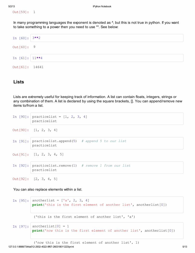
In many programming languages the exponent is denoted as , but this is not true in python. If you want

to take something to a power then you need to use **. See below:

In [60]:

In [61]:

Lists

Lists are extremely useful for keeping track of information. A list can contain floats, integers, strings or

any combination of them. A list is declared by using the square brackets, []. You can append/remove new

items to/from a list.

In [90]:

In [91]:

In [92]:

You can also replace elements within a list.

In [95]:

In [97]:

Out[59]: 1

3**2

Out[60]: 9

11**4

Out[61]: 14641

practicelist = [1, 2, 3, 4]practicelist

Out[90]: [1, 2, 3, 4]

practicelist.append(5) # append 5 to our listpracticelist

Out[91]: [1, 2, 3, 4, 5]

practicelist.remove(1) # remove 1 from our listpracticelist

Out[92]: [2, 3, 4, 5]

anotherlist = ['a', 2, 3, 4]print('this is the first element of another list', anotherlist[0])

('this is the first element of another list', 'a')

anotherlist[0] = 1print('now this is the first element of another list', anotherlist[0])

('now this is the first element of another list', 1)


127.0.0.1:8888/7344a512-2932-4022-8f67-260318011223/print 6/13

Taking slices of lists works the same way as taking slices of strings.

In [99]:

We can also concatenate lists just like we did with strings.

In [93]:

In addition to being able to do these things that you were able to do in a string, lists allow you to find the

max and min (among other things) within the list.

In [108]:

One of the built in commands to build lists is with the range command. Below we will build a list of

numbers from 0 to 9 using range in several different ways.

In [100]:

In [101]:

In [102]:

Conditionals, Loops, and Booleans

('now this is the first element of another list', 1)

list1 = [1, 2, 3, 4, 5, 6, 7]list1[2:5] # take elements 2 through 5

Out[99]: [3, 4, 5]

list1 = [1, 2]list2 = ['a', 'b']list1 + list2

Out[93]: [1, 2, 'a', 'b']

list1 = [1, 2, 36, 256, 2562, 56]print('The max is %s' %max(list1))print('The min is %s' %min(list1))

The max is 2562The min is 1

range(10) # if you just input an integer it will build up until that number

Out[100]: [0, 1, 2, 3, 4, 5, 6, 7, 8, 9]

range(0,10,1) # you can tell it to start at 0 and go to 10 taking 1 unit steps

Out[101]: [0, 1, 2, 3, 4, 5, 6, 7, 8, 9]

range(1,10) # we can go from 1 to 9 as well by specifying to start at 1

Out[102]: [1, 2, 3, 4, 5, 6, 7, 8, 9]


127.0.0.1:8888/7344a512-2932-4022-8f67-260318011223/print 7/13

Conditional statements, loops, and booleans permit a programmer increased flexibility. These permit you

to give your computer specific commands that save you a lot of coding. For example, if you want to

remove all of the even numbers from a list then you can say something like below:

Also some symbols that will be useful: < less than

greater than <= less than or equal = greater than or equal != not equal == equal to

In [113]:

In [112]:

Booleans are just values tied to certain expressions that evaluate to either true or false. If and while

statements are evaluated based on these values. For example, below we said 5 < 3 and the computer

says False because that isn't true

In [117]:

The conditional statements that you should be most familiar with are "if/elif/else" and "while". They are

used exactly how you would imagine that they are used. You want to tell the computer if something is true

then do this, else do this other thing. You could also tell your computer while this condition is true then

continue doing what I told you to do. Below are two examples (Note where the indentations (done by

inserting 4 spaces) are):

In [118]:

In [115]:

list1 = range(25)print(list1)

[0, 1, 2, 3, 4, 5, 6, 7, 8, 9, 10, 11, 12, 13, 14, 15, 16, 17, 18, 19, 20, 21, 22, 23, 24]

list2 = [list1[n] for n in list1 if n%2!=0] # This removes all even numbersprint(list2)

[1, 3, 5, 7, 9, 11, 13, 15, 17, 19, 21, 23]

5 < 3

Out[117]: False

x = 3if x < 3: print('x is less than 3')elif x < 4: print('x is less than 4')else: print('x is not less than 4')x is less than 4

x = 1while x < 7: print('x is still less than 7') x = x + 1 # Increase x by 1

x is still less than 7x is still less than 7


127.0.0.1:8888/7344a512-2932-4022-8f67-260318011223/print 8/13

For conditional statements, if you are asking whether something is equal you need to use two =. This is

because python thinks one = means that you are setting something equal to that, but you are asking

whether it is or isn't. See example:

In [124]:

Looping is a very similar to a while loop, but you give it a specific number of times it should do something.

For example if we had a list and we wanted to square every element, we could use a for loop.

In [121]:

Developing a Function and Exploring Modules

Python Modules

One of the biggest benefits of python is the fact that it is open source. This means that there are almost

constanly individuals contributing to python to build modules. Modules are just files that contain python

code that you are able to use. Some of the modules that you will use very frequently are: math, numpy,

pandas, byumcl, and other modules you might write for yourself. Although you will use these most, if you

ever think that something would be nice to be able to do then most likely someone has written a module

that does that task. Once again, google will be your best friend in finding these.

You need to import modules into your session to be able to use them. You need to do all of your imports

at the very beginning when you are writing a script. These imports are done like this:

In [106]:

x is still less than 7x is still less than 7x is still less than 7x is still less than 7

x = 6if x == 6: print('told ya so :)')

told ya so :)

list1 = [1, 2, 3, 4, 5, 6] for i in range(len(list1)): # len(list1) tells us how many elements we need to loop on list1[i] = list1[i]**2 # The ith element of list1 = (ith element of list1) ^2 print('list1 squared is %s' %list1)

list1 squared is [1, 4, 9, 16, 25, 36]

import numpy as np # the 'as np' part creates a nickname for functions from this moduleimport mathimport osfrom filename import * # will import functions that you have written in another script


127.0.0.1:8888/7344a512-2932-4022-8f67-260318011223/print 9/13

You have to refer to the module you just imported in order to call an object from that module. For

example: We wrote math.pi in the code above. This tells python to look in the math module and call the

function pi. When we write things like the "import numpy as np", we are giving numpy a nickname and we

can write np.numpy_function instead of writing numpy.numpy_function. It is also helpful to try

help(module) to see if you can find documentation. You can also use module.object(?? to open the

documentation for a specific object in a module.

Defining Functions

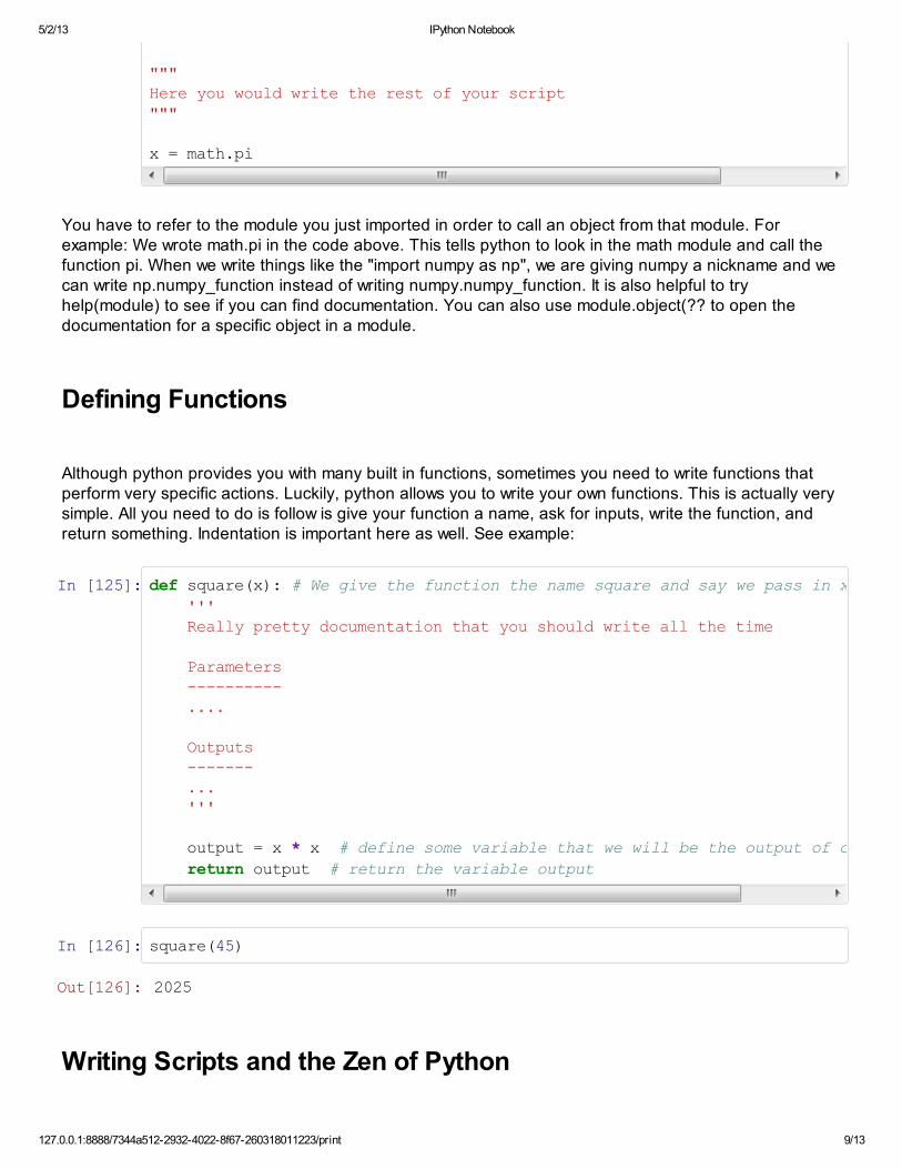
Although python provides you with many built in functions, sometimes you need to write functions that

perform very specific actions. Luckily, python allows you to write your own functions. This is actually very

simple. All you need to do is follow is give your function a name, ask for inputs, write the function, and

return something. Indentation is important here as well. See example:

In [125]:

In [126]:

Writing Scripts and the Zen of Python

"""Here you would write the rest of your script""" x = math.pi

def square(x): # We give the function the name square and say we pass in x ''' Really pretty documentation that you should write all the time Parameters ---------- .... Outputs ------- ... ''' output = x * x # define some variable that we will be the output of our function return output # return the variable output

square(45)

Out[126]: 2025


127.0.0.1:8888/7344a512-2932-4022-8f67-260318011223/print 10/13

Writing a Script

Writing a script is pretty simple, so I will try and go over it pretty quick. A script should start with all of your

imports and then you write your code. It should be neat and you should leave one clean line at the end of

your script or the code monster will come and eat you. Example of a script:

In [128]:

After you have written a script then you need to enter your ipython console. From there, direct your

computer to the directory where the script is stored and type "run script.py" That's it for running scripts.

Zen of Python (PEP 20)

The Zen of Python is a set of basic rules that one should follow when writing python code. They are

important to follow as they will make your code readable and will bring good code karma to you and your

family. Anytime that you forget these rules, type "import this" into your console.

Beautiful is better than ugly.

Explicit is better than implicit.

Simple is better than complex.

Complex is better than complicated.

Flat is better than nested.

Sparse is better than dense.

Readability counts.

Special cases aren't special enough to break the rules.

Although practicality beats purity.

Errors should never pass silently.

Unless explicitly silenced.

In the face of ambiguity, refuse the temptation to guess.

There should be one-- and preferably only one --obvious way to do it.

import mathimport osfrom __future__ import division x = 2.0 y = x * math.pi finalstuff = square(y)


127.0.0.1:8888/7344a512-2932-4022-8f67-260318011223/print 11/13

Although that way may not be obvious at first unless you're Dutch.

Now is better than never.

Although never is often better than right now.

If the implementation is hard to explain, it's a bad idea.

If the implementation is easy to explain, it may be a good idea.

Namespaces are one honking great idea -- let's do more of those!

In [129]:

Style Guide for Python (PEP 8)

PEP 8 is too long to put into this document, but I would highly suggest reading through it. The

suggestions in PEP 8 are very helpful in making your code readable and in line with the Zen of Python. I

will include a few of the tips that I find important.

Indentation: Use 4 spaces per indentation level. Python's implicit line joining inside parentheses,brackets and braces, or using a hanging indent. When using a hanging indent the following

considerations should be applied;; there should be no arguments on the first line and further indentation

should be used to clearly distinguish itself as a continuation line.

Maximum Line Length: Limit all lines to a maximum of 79 characters.

Blank Lines: Separate top-level function and class definitions with two blank lines. Method definitionsinside a class are separated by a single blank line. Extra blank lines may be used (sparingly) to separate

groups of related functions. Blank lines may be omitted between a bunch of related one-liners (e.g. a set

import this

The Zen of Python, by Tim Peters

Beautiful is better than ugly.Explicit is better than implicit.Simple is better than complex.Complex is better than complicated.Flat is better than nested.Sparse is better than dense.Readability counts.Special cases aren't special enough to break the rules.Although practicality beats purity.Errors should never pass silently.Unless explicitly silenced.In the face of ambiguity, refuse the temptation to guess.There should be one-- and preferably only one --obvious way to do it.Although that way may not be obvious at first unless you're Dutch.Now is better than never.Although never is often better than *right* now.If the implementation is hard to explain, it's a bad idea.If the implementation is easy to explain, it may be a good idea.Namespaces are one honking great idea -- let's do more of those!


127.0.0.1:8888/7344a512-2932-4022-8f67-260318011223/print 12/13

of dummy implementations).

Whitespace in Expressions: Avoid extraneous whitespace in the following situations: Immediatelyinside parentheses, brackets or braces;; Immediately before a comma, semicolon, or colon, Immediately

before the open parenthesis that starts the argument list of a function call, Immediately before the open

parenthesis that starts an indexing or slicing, More than one space around an assignment (or other)

operator to align it with another. If operators with different priorities are used, consider adding whitespace

around the operators with the lowest priority(ies). Use your own judgement;; however, never use more

than one space, and always have the same amount of whitespace on both sides of a binary operator.

For example:

Yes

In [130]:

No

In [ ]:

Comments: Comments that contradict the code are worse than no comments. Always update comments!Comments should be complete sentences.

We are hoping to edit your code and give you tips on how to make it stay consistent with PEP 8 and PEP

20. We recommend using the sublime_linter in Sublimetext 2 to stay in line with PEP 8.

Problems:

All scripts submitted should obviously be in line with PEP 8 and PEP 20 for this assignment because that

is one of the topics covered. Include comments.

Problem 1: Write a script that generates the following:

i) A list with all of the elements from 0 to 100

ii) A list with all of the even elements from 0 to 100

iii) A list that contains all of the even numbers starting at 100 and going to 0

Problem 2: Write a script that creates a piecewise function f(x) = y that satisfies the following:

x = 0x += 1x = x + 1x = x**2 + 2test = x*x + 2*xy = (x+2) * (x-3)

x=x+1x +=1x = 2 * x + 1y = (x + 2) * (x - 3)


127.0.0.1:8888/7344a512-2932-4022-8f67-260318011223/print 13/13

i) When x < 0 then y = 0

ii) When 0 < x <=5 then y = x*x

iii) When x > 5 then y = 25

iv) Now copy the following code to create a plot

In [132]:

Problem 3: If we list all the natural numbers below 10 that are multiples of 3 or 5, we get 3, 5, 6 and 9.The sum of these multiples is 23.

Write a script that prints the sum of all the multiples of 3 or 5 below 1000.

In [ ]:

import matplotlib.pyplot as plt# Define function in here

test = range(-10, 15, 1)plt.plot(f(test)) # Note this isn't your actual function being plotted below.

Out[132]: [<matplotlib.lines.Line2D at 0x7070828>]

Lab 3

Essentials: NumPy

Why Arrays?

Problem 1 Let’s begin with a simple demonstration of why arrays are importantfor numerical computation. Why use arrays when Python already has decentlyecient list object? In this demonstration, we will try squaring a matrix. Thematrix will be represented as a two dimensional list (i.e. a list of lists).

Write a function that will accept two matrices (two dimensional list), A andB, and return AB following the rules of matrix multiplication.

k = 10

a = [range(i, i+k) for i in range(0, k**2, k)]

Time how long your function takes to square matrices for increasing values of k.Now import NumPy and create a NumPy array, b as shown below. We demon-

strate how to square NumPy arrays as matrices below. b*b does not square the array,but rather multiplies b with itself element-wise. To get matrix multiplication forNumPy arrays, you must use np.dot

import numpy as np

b = np.array([range(i, i+k) for i in range(0, k**2, k)])

np.dot(b, b)

Time how long NumPy takes to square arrays for increasing sizes of k.What do you notice about the time needed to square a two dimensional list

vs. a two dimensional NumPy array?

NumPyNumPy is a fundamental package for scientific computing with Python. It providesan ecient n-dimensional array object for fast computations. This lab will focus on

19

20 Lab 3. NumPy

how to use these powerful objects. NumPy is commonly imported as shown below.

: import numpy as np

Before beginning this lab, it will be useful to understand certain concepts and termsused to describe NumPy arrays.

N-Dimensions

One, two, and three dimensional arrays are easy to visualize. But how do wevisualize a four, ten, or fifteen dimensional array? NumPy arrays are best thoughtof as arrays within arrays. A one dimensional array consists of only elements. A twodimensional array is really just an array containing arrays which contain elements.Extending this metaphor, a three dimensional array is an array of arrays of arrays.Can you guess what a five dimensional array is? Let’s define a three dimensionalarray.

: arr = np.random.randint (50, size=(5, 4, 3))

Arrays have several attributes. We use shape and size to describe the how bigan array is. Shape tells how how many dimensions an array has and how big eachdimension is. Size gives the total number of elements in the array.

: arr.shape

(5, 4, 3)

: arr.size

60

If we want to know how much memory an array takes to store, we can usearr.nbytes. The number of bytes is dependent on the data type (dtype) of the array.The data types that NumPy uses are di↵erent from Python data types. An integerin NumPy is not the same as an integer Python. Remembering this is vital. NumPyuses machine data types to speed up calculations. However, these datatypes are sus-ceptible to a problem called overflow. A 64 bit integer has enough bits to representintegers between 9, 223, 372, 036, 854, 775, 808 and 9, 223, 372, 036, 854, 775, 807. Ifwe have an array with 9, 223, 372, 036, 854, 775, 808 and we decide to subtract 1,the integer wraps around and becomes 9, 223, 372, 036, 854, 775, 807!

: arr.dtype

dtype(’int64’)

: arr.nbytes

480

Each element of the array has a unique address that describes it location.Indexing always starts at 0. Also, like Python lists, negative indices are valid andcount from the tail of the array. We will discuss indexing in detail later in this lab.

: arr[0, 0, 0] # returns the first element of arr

: arr[-1, -1, -1] #returns the last element of arr

21

Creating ArraysNumPy has several methods for creating and initializing arrays. When creating anarray, we can optionally specify the data type that is stored in the array. NumPyarrays only store elements of the same data type, however, that data type can beany arbitrary object. The array order dictates how the array is laid out in memory.There is C order and Fortran order. C ordered arrays are also known as row-majorarrays. This means that the fastest changing index correspond to the rows of thearray. Fortran ordered arrays are column-major. Let’s look at a few of the ways wecan create arrays in NumPy.

• np.array: Makes an array from a Python list or tuple.

• np.empty: Allocates an array of a specific size without initializing the elements.

• np.ones: Allocates and array and initializes each element to 1.

• np.zeros: Allocates and array and initializes each element to 0.

• np.identity: Allocates a 2D array array with the main diagonal initialized to1 and zeros everywhere else.

Indexing Arrays

Array Views and Copies

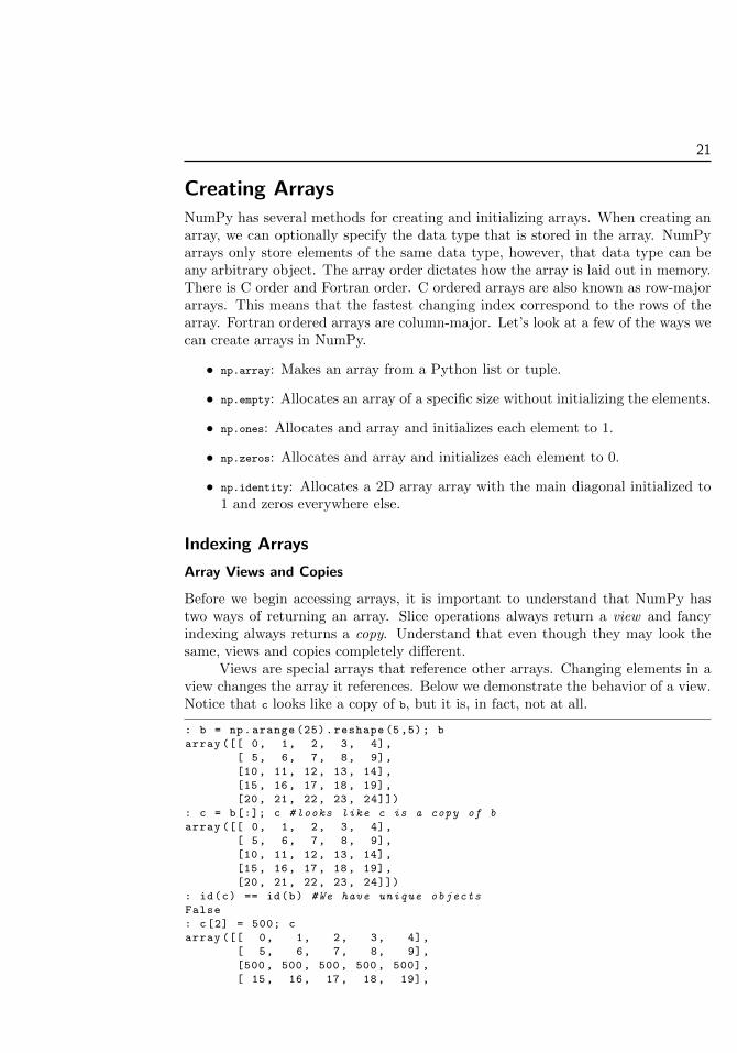
Before we begin accessing arrays, it is important to understand that NumPy hastwo ways of returning an array. Slice operations always return a view and fancyindexing always returns a copy. Understand that even though they may look thesame, views and copies completely di↵erent.

Views are special arrays that reference other arrays. Changing elements in aview changes the array it references. Below we demonstrate the behavior of a view.Notice that c looks like a copy of b, but it is, in fact, not at all.

: b = np.arange (25).reshape (5,5); b

array ([[ 0, 1, 2, 3, 4],

[ 5, 6, 7, 8, 9],

[10, 11, 12, 13, 14],

[15, 16, 17, 18, 19],

[20, 21, 22, 23, 24]])

: c = b[:]; c #looks like c is a copy of b

array ([[ 0, 1, 2, 3, 4],

[ 5, 6, 7, 8, 9],

[10, 11, 12, 13, 14],

[15, 16, 17, 18, 19],

[20, 21, 22, 23, 24]])

: id(c) == id(b) #We have unique objects

False

: c[2] = 500; c

array ([[ 0, 1, 2, 3, 4],

[ 5, 6, 7, 8, 9],

[500, 500, 500, 500, 500],

[ 15, 16, 17, 18, 19],

22 Lab 3. NumPy

[ 20, 21, 22, 23, 24]])

: b #changing c also changed b!

array ([[ 0, 1, 2, 3, 4],

[ 5, 6, 7, 8, 9],

[500, 500, 500, 500, 500],

[ 15, 16, 17, 18, 19],

[ 20, 21, 22, 23, 24]])

The reason that changing the array c also changed the array b is because c andb share the same memory, even though they are di↵erent Python objects. Viewsreduce the overhead of making copies of arrays and are useful when we want tochange certain parts of the array.

A copy of an array is a separate array that is allocated separately.

: b = np.arange (25).reshape(5, 5); b

array ([[ 0, 1, 2, 3, 4],

[ 5, 6, 7, 8, 9],

[10, 11, 12, 13, 14],

[15, 16, 17, 18, 19],

[20, 21, 22, 23, 24]])

: c = b.copy()

: id(c) == id(b) #we still have separate objects

False

: c[2] = 500

array ([[ 0, 1, 2, 3, 4],

[ 5, 6, 7, 8, 9],

[500, 500, 500, 500, 500],

[ 15, 16, 17, 18, 19],

[ 20, 21, 22, 23, 24]])

: b

array ([[ 0, 1, 2, 3, 4],

[ 5, 6, 7, 8, 9],

[10, 11, 12, 13, 14],

[15, 16, 17, 18, 19],

[20, 21, 22, 23, 24]])

Changing the data in a copy of an array, doesn’t change the data in the originalarray. The two arrays address di↵erent locations in memory.

Slices

Each element of an array has a unique address that we can use to retrieve thatelement. Indexing NumPy arrays is syntatically the same as indexing Python lists.We will demonstrate on a random 2D array. Remember that slicing arrays alwaysreturn views of the array. In this case, the indexing object is a Python tuple.

: arr = np.arange (25).reshape (5,5); arr

array ([[ 0, 1, 2, 3, 4],

[ 5, 6, 7, 8, 9],

[10, 11, 12, 13, 14],

[15, 16, 17, 18, 19],

[20, 21, 22, 23, 24]])

: arr[0, 0] #access the first element

0

: arr[-1, -1] #access the last element

23

24

: arr[0] #access the first row

array([0, 1, 2, 3, 4])

We can access ranges of elements using Python lists. NumPy, though, has a muchfaster, more concise way to select ranges using the arr[start:stop:step] notation.

: arr [::2] #get every other row. equivalent to arr[range (0, len(arr),

2)]

array ([[ 0, 1, 2, 3, 4],

[10, 11, 12, 13, 14],

[20, 21, 22, 23, 24]])

: arr[::2, ::2] #get every other row and every other column

array ([[ 0, 2, 4],

[10, 12, 14],

[20, 22, 24]])

: arr[3:, 3:] #extract lower right 2x2 subarray

array ([[18, 19],

[23, 24]])

: arr[:, 1] #extract second column

array([ 1, 6, 11, 16, 21])

Fancy Indexing

When the indexing object is an object other than a tuple, NumPy behaves slightlydi↵erent. One di↵erence is that fancy indexes always return a copy of an array in-stead of a view. There are two types of fancy indexes: boolean and integer. Booleanindexing returns an array of True or False values depending on some evaluating con-dition.

: bmask = (arr > 15) & (arr < 23)

array ([[False , False , False , False , False],

[False , False , False , False , False],

[False , False , False , False , False],

[False , True , True , True , True],

[ True , True , True , False , False]], dtype=bool)

: arr[bmask]

array ([16, 17, 18, 19, 20, 21, 22])

: arr[(arr > 15) & (arr < 23)] #this is the shortened form

array ([16, 17, 18, 19, 20, 21, 22])

: arr[~bmask] #invert the mask

: arr[(0, 2, 4), (0, 2, 4)] #grab every other element of diagonal

array([ 0, 12, 24])

: arr[range(0, 5, 2), range(0, 5, 2)] #same as above , but with ranges

array([ 0, 12, 24])

: arr[:, [0, -1]] #grab first and last column

array ([[ 0, 4],

[ 5, 9],

[10, 14],

[15, 19],

[20, 24]])

24 Lab 3. NumPy

Array BroadcastingArray broadcasting allows NumPy to e↵ectively work with arrays with sizes thatdon’t match exactly. There are four basic rules to determine the behavior of broad-casted arrays

1. All input arrays of lesser dimension than the input array with largest dimen-sion have 1’s prepended to their shapes.

2. The size in each dimension of the output shape is the maximum of all theinput sizes in that dimension.

3. An input can be used in the calculation if its size in a particular dimensioneither matches the output size in that dimension, or has a value exactly 1.

4. If an input has a dimension size of 1 in its shape, the first data entry in thatdimension will be used for all calculations along that dimension.

To broadcast arrays, at least one of the following must be true.

1. All input arrays have exactly the same shape.

2. All input arrays are of the same dimension and the length of correspondingdimensions match or is 1.

3. All input arrays of fewer dimension can have 1 prepended to their shapes tosatisfy the second criteria.

Problem 2 Explore array broadcasting. Create example for each of the three caseswhere arrays are broadcasted.

Saving ArraysSometimes it is desirable to save an array to a file to be used for later. NumPyprovides several easy to use methods for saving and loading array data to files.

np.save(file, arr) Save an array to a binary filenp.savez(file, *arrs) Save multiple arrays to a binary filenp.savetxt(file, arr) Save an array to a text file

np.load(file) Load and return an array from a binary filenp.loadtxt(file) Load and return an array from text file

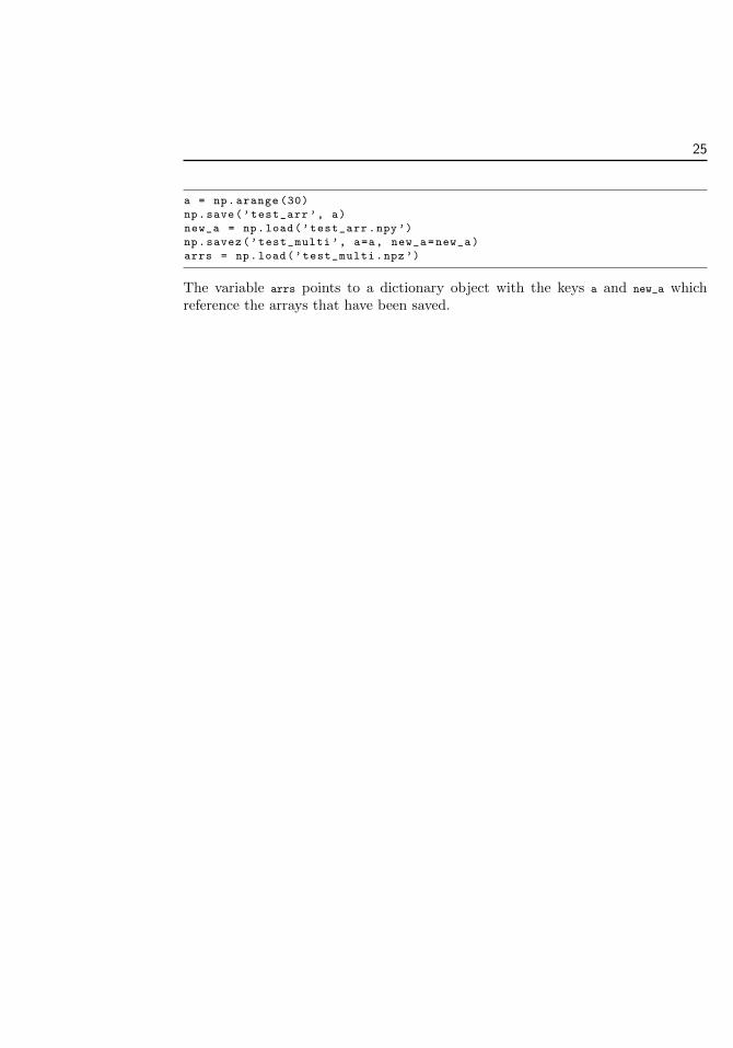
Let’s practice saving an array to a file and loading it again. Note that whensaving an array, NumPy automatically appends the extension .npy if it does notalready exist.

25

a = np.arange (30)

np.save(’test_arr ’, a)

new_a = np.load(’test_arr.npy’)

np.savez(’test_multi ’, a=a, new_a=new_a)

arrs = np.load(’test_multi.npz’)

The variable arrs points to a dictionary object with the keys a and new_a whichreference the arrays that have been saved.

Lab 4

Algorithms: PythonEssentials (Arrays)

Lesson Objective: This lesson explains basic matrix operations in Python.

Matrices form the core data structure of NumPy and SciPy. Thus, we willexplore the ways one can manipulate matrices in Python.

Before we begin, we make a few important comments about how Python workswith matrices. First, matrices can be represented in NumPy in two ways. NumPyhas a matrix data type and an array data type. Matrix objects are a special caseof the array object. The main di↵erences are that the matrix object allows fora clearer, more MATLAB style syntax. In these labs, we will use arrays becausemost functions in NumPy accept arrays as input. We can easily convert arrays tomatrices using the .asmatrix() method. As such, all future references to matricesin the context of NumPy will be mentioned as arrays (a matrix being a 2D array).When using arrays it is important to be sure that the dimensions are compatible.

We also note that arrays are by default are accessed row by row. This is calledrow-major. This is the opposite of MATLAB, which is column-major. However,NumPy arrays can converted to column-major arrays.

Finally, with all code examples in these labs we assume that you have alreadyimported the SciPy library (type import scipy as sp when you first open ipython).

To begin, we will work with vectors. We will demonstrate a variety of methodsto create vectors. You should follow these demonstrations on your own computerand experiment as you go. Vectors are at least one dimensional arrays. There areseveral ways to create vectors in Python. Try the following in IPython:

: a = sp.array ([1,2,3,4]); a

array([1, 2, 3, 4])

Notice the square brackets and the commas. The square brackets denote alist in Python with values separated by commas. This is a row vector. The ; a isresponsible for printing the current value of a. How do we make a column vector?We simply pass the array() method a list of lists containing a single value each.

29

30 Lab 4. Python Essentials (Arrays)

: b = sp.array ([[3] ,[4] ,[6] ,[1]]); b

array ([[3],

[4],

[6],

[1]])

We can also use the hstack() and vstack() methods (meaning horizontal stackand vertical stack).

: a1 = sp.hstack ([5,6,7,8])

: b1 = sp.vstack ([9,0,1,2])

We combine vectors together by placing two or more of equal dimension insidesquare brackets. The technical term for this is concatenation. Remember that thedimensions of each array must match. Try the following.

: c = sp.concatenate ((b,b1), axis =1); c

There are several methods to automate vector creation. For example, we canbuild a vector of consecutive values using the arange() method.

: sp.arange (5)

Notice how the values start at zero and increment up to, but not including 5.This is standard Python behaviour. The arange() method also allows us to specifiystep size This syntax also allows us to specify step size:

: sp.arange(1,3,step =0.5)

We can similarly use negative step sizes (note that the starting must be greaterthan the endpoint).

: sp.arange(3,1, step =-.5)

A related function is called linspace(). It allows us to specify two endpointsand the number of equidistant values we want between the two. Unlike arange(),linspace() will always include both endpoints.

: sp.linspace (1,2,5)

The plot() function uses two vectors to create a graph, the first vector rep-resenting x-values and the second representing the corresponding y-values. To useplot(), we need to import the Matplotlib library. As an example we plot a line ofslope two using the following commands (See figure 1.1):

: import matplotlib.pyplot as plt

: x = sp.linspace (-2,2,20)

: plt.plot(x,2*x)

: plt.show()

By typing plt.plot? into the command line we can find the exact syntax andoptions for the plot() function. For example we can type plot(x,2*x,’r*’) to plotred star data points instead of a line.

31

Figure 4.1: A simple graph

Problem 1 Plot a line with slope three with black diamond data points. Plot forthe domain x 2 [5, 5].

Creating is done by concatenating vectors in the correct manner. For example:

: sp.array ([[1, 2, 3],[4, 5, 6],[7, 8, 9]])

Problem 2 Create a matrix showing the times table from 1 to 6. Do not enter eachnumber manually. Instead, create a variable x = sp.arange(1,7) and let the rows ofthe matrix be multiples of x.

Another technique for creating matrices is using outer products. An outerproduct is the method of multiplying two vectors to get a matrix. For example, ifwe want to make a matrix that is two repeated rows of the vector 1:5 we can dothe following:

: sp.vstack ([1 ,1])*sp.arange (1,6)


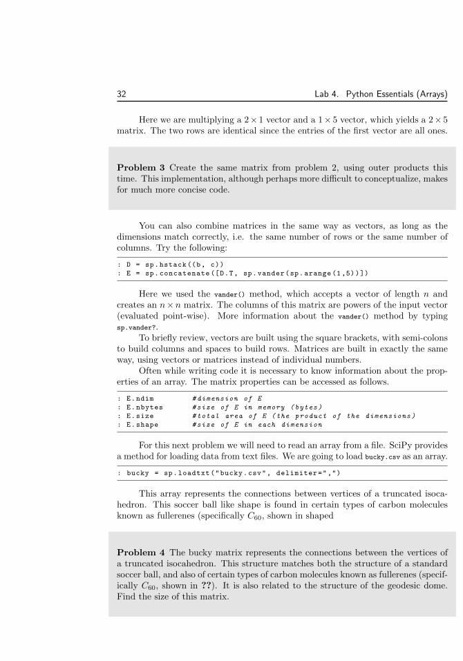
Here we are multiplying a 2 1 vector and a 1 5 vector, which yields a 2 5matrix. The two rows are identical since the entries of the first vector are all ones.

Problem 3 Create the same matrix from problem 2, using outer products thistime. This implementation, although perhaps more dicult to conceptualize, makesfor much more concise code.

You can also combine matrices in the same way as vectors, as long as thedimensions match correctly, i.e. the same number of rows or the same number ofcolumns. Try the following:

: D = sp.hstack ((b, c))

: E = sp.concatenate ([D.T, sp.vander(sp.arange (1,5))])

Here we used the vander() method, which accepts a vector of length n andcreates an nn matrix. The columns of this matrix are powers of the input vector(evaluated point-wise). More information about the vander() method by typingsp.vander?.

To briefly review, vectors are built using the square brackets, with semi-colonsto build columns and spaces to build rows. Matrices are built in exactly the sameway, using vectors or matrices instead of individual numbers.

Often while writing code it is necessary to know information about the prop-erties of an array. The matrix properties can be accessed as follows.

: E.ndim #dimension of E

: E.nbytes #size of E in memory (bytes)

: E.size #total area of E (the product of the dimensions )

: E.shape #size of E in each dimension

For this next problem we will need to read an array from a file. SciPy providesa method for loading data from text files. We are going to load bucky.csv as an array.

: bucky = sp.loadtxt("bucky.csv", delimiter=",")

This array represents the connections between vertices of a truncated isoca-hedron. This soccer ball like shape is found in certain types of carbon moleculesknown as fullerenes (specifically C60, shown in shaped

Problem 4 The bucky matrix represents the connections between the vertices ofa truncated isocahedron. This structure matches both the structure of a standardsoccer ball, and also of certain types of carbon molecules known as fullerenes (specif-ically C60, shown in ??). It is also related to the structure of the geodesic dome.Find the size of this matrix.

33

Figure 4.2: The structure of the C60 molecule.

To access information in an array, you put the index you wish to access insidesquare brackets after the variable name. This works for both variable assignmentand retrieval. Remember that indices start at zero in SciPy.

: rand_mat = sp.random.randint (10, size =(3 ,5))

: rand_mat [0,0]

: rand_mat [2,2] = 37

The colon operator is used to retrieve an entire row or column from an array.For example, enter the following to get the third column of an array:

: rand_mat [:,2]

We similarly retrieve the first row:

: rand_mat [0,:]

Note that each retrieved row or column is returned as a single dimensionalarray (meaning that row or column loses it meaning). If we want to retain theretrieved row as a column or row we can write instead rand_mat[:,[2]].

It is also possible to retrieve multiple columns or rows at once. For example,we retrieve the second and fourth columns of an array by entering:

: rand_mat [:,[1 ,3]]

We list the entries of an array as a single dimensional array using the flatten()method.

: rand_mat.flatten () #flattens along the rows (C like arrays)

: rand_mat. flatten(’F’) #flattens along the columns (Fortran like

arrays)

The following line tells Python to retrieve the entries in the second row, fromthe second column to the end:

: rand_mat [1,1:]


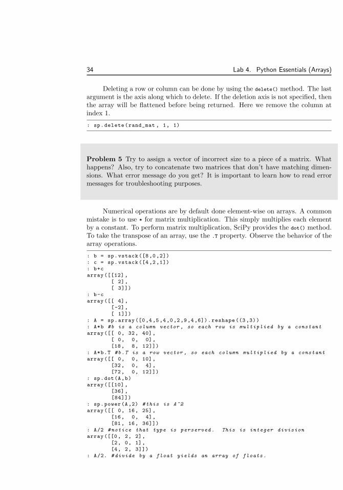
Deleting a row or column can be done by using the delete() method. The lastargument is the axis along which to delete. If the deletion axis is not specified, thenthe array will be flattened before being returned. Here we remove the column atindex 1.

: sp.delete(rand_mat , 1, 1)

Problem 5 Try to assign a vector of incorrect size to a piece of a matrix. Whathappens? Also, try to concatenate two matrices that don’t have matching dimen-sions. What error message do you get? It is important to learn how to read errormessages for troubleshooting purposes.

Numerical operations are by default done element-wise on arrays. A commonmistake is to use * for matrix multiplication. This simply multiplies each elementby a constant. To perform matrix multiplication, SciPy provides the dot() method.To take the transpose of an array, use the .T property. Observe the behavior of thearray operations.

: b = sp.vstack ([8 ,0 ,2])

: c = sp.vstack ([4 ,2 ,1])

: b+c

array ([[12] ,

[ 2],

[ 3]])

: b-c

array ([[ 4],

[-2],

[ 1]])

: A = sp.array ([0,4,5,4,0,2,9,4,6]).reshape ((3 ,3))

: A*b #b is a column vector , so each row is multiplied by a constant

array ([[ 0, 32, 40],

[ 0, 0, 0],

[18, 8, 12]])

: A*b.T #b.T is a row vector , so each column multiplied by a constant

array ([[ 0, 0, 10],

[32, 0, 4],

[72, 0, 12]])

: sp.dot(A,b)

array ([[10] ,

[36],

[84]])

: sp.power(A,2) #this is A^2

array ([[ 0, 16, 25],

[16, 0, 4],

[81, 16, 36]])

: A/2 #notice that type is perserved. This is integer division

array ([[0, 2, 2],

[2, 0, 1],

[4, 2, 3]])

: A/2. #divide by a float yields an array of floats.

35

array ([[ 0. , 2. , 2.5],

[ 2. , 0. , 1. ],

[ 4.5, 2. , 3. ]])

The majority of elementary functions, such as sin, cos, exp, etc. act element-wise on arrays as well. In fact, for any operation in SciPy, expect it to act element-wise unless otherwise noted. For example:

: sp.sin(sp.arange (4)*sp.pi/4)

array([ 0. , 0.70710678 , 1. , 0.70710678])

Also, as a matter of reference, raising a value to a power is done using **. Thisis a convention from older programming languages that has carried over.

There are a variety of functions that let us summarize information about agiven array. For example, the sum() function returns the sum along a given axisof an array. When an axis is not specified, all elements in the array are summedtogether.

: B = sp.arange (9).reshape ((3 ,3))

: sp.sum(B) #all entries are summed together

36

: sp.sum(B, axis =0) #sum each column

array([ 9, 12, 15])

: sp.sum(B, axis =1) #sum each row

array([ 3, 12, 21])

Some other functions that summarize information about the entries of anarray are contained in the Table 1.1. Note that each of these functions reducesthe size of the matrix (which makes sense, since they are summarizing functions).These functions work across columns by default, although most of them allow youto specify an axis to work across.

These functions can be incredibly useful. For example, suppose that we wantto estimate the derivative of sin(x2). A simple approximation for a derivative is

f 0(x) f(x+ h) f(x)

h

Presumably this approximation is good when h is small. We use the diff()

function to perform this approximation using the following code:

: h = .001

: x = sp.arange(0,sp.pi,h)

: approx = sp.diff(sp.sin(x**2))/h

We have just approximated the derivative of sinx2 at several thousand pointsbetween 0 and . The approximated derivatives are stored in the array approx. Nowlet’s compute the actual derivative at each point using the formula:

f 0(x) = 2xcos(x2)

: actual = 2*sp.cos(x**2)*x;


Function Description Usagemax Returns maximum entries A.max(axis)min Returns mimimum entries A.min(axis)mean Returns the mean A.mean(axis)scipy.median Returns the median sp.median(A, axis)std Returns the standard de-

viationA.std(axis)

scipy.diff Returns the di↵erencesbetween entries

sp.di↵(A, axis)

prod Returns the product of en-tries

A.prod(axis)

any Returns 1 if there are non-zero entries, zero other-wise

A.any(axis)

all Returns 1 if all entries arenon-zero, zero otherwise

A.all(axis)

nonzero Returns indices of non-zero entries

A.nonzero(axis)

scipy.linalg.norm Returns the norm norm(A, order)

Table 4.1: Various summarizing functions

Plot the approximated derivative and the actual derivative on two di↵erentplots. They should look almost identical.

: from matplotlib import pyplot as plt

: plt.figure (1) #create an empty figure

: plt.subplot (211) #create an empty subplot in figure

: plt.plot(x, approx)

: plt.subplot (212) #create another subplot in same figure

: plt.plot(x, actual)

: plt.show()

Problem 6 Now use the max() command to find the maximum di↵erence betweenthe estimated derivative and the actual derivative (the dimensions will not matchexactly (why?); fix this by removing the last entry from one of the vectors). Tryplotting the approximation, actual deriviatives, and the error on the same graph.What does it look like?

Problem 7 The command sp.rand() returns an array of a specified shape with val-ues “randomly” selected from a uniform distribution between zero and one. Create

37

a vector with ten thousand entries using this command. The theoretical values forthe mean(µ) and standard deviation() of a uniformly distributed random variablebetween a and b are

µ =a+ b

2

=b ap

12

These values are calculated using moment-generating functions. Use the mean() andstd() methods on the vector you created earlier. How do these compare to thetheoretical values?

The canonical problem in linear algebra is solving the equation Ax = b for x,where A is an n n matrix and b is a 1 n vector. One method for solving thisequation is by calculating the matrix inverse of A (A1) and multiplying A1b. Tofind the inverse of an array, use the linalg.inv() method. For example, we createa random system Ax = b and solve it using the inv() method (you may check thecalculations by hand):

: A = sp.array ([1,5,2,3,5,1,4,7,2]).reshape ((3 ,3))

: b = sp.vstack ([1, 3, 11./3])

: from scipy import linalg as la

: sol = sp.dot(la.inv(A),b); sol

array ([[ 0.66666667] ,

[ 0.33333333] ,

[ -0.66666667]])

Recall that a norm is a measurement on the size of a vector. For example, theEuclidean norm measures the straight line distance from the origin to the “end” ofa vector.

kxk =q

x21 + ...+ x2

n

If the norm of the di↵erence of two vectors is close to zero, then they are goodapproximations of each other. The linalg.norm() function calculates the euclideannorm of an input vector, and thus we use it to verify that our approximation of thederivative is close to the actual derivative:

: la.norm(b-sp.dot(A,sol))

5.5288660751834285e-15

However, computing the inverse of a large matrix is dicult. Not only that,but not all matrices have inverses. There is a much more ecient and general wayto solve Ax = b in SciPy. This method is similar to the backslash method found inMATLAB. It is the linalg.solve() method. Compare the results obtained with thelinalg.solve() method to those of the linalg.inv() method.


: sol2 = la.solve(A,b); sol2

array ([[ 0.66666667] ,

[ 0.33333333] ,

[ -0.66666667]])

: la.norm(sol2 -sol)

4.5775667985222375e-16

We mentioned that linalg.solve() is more ecient than using the functioninv, meaning it returns a result faster. Create the following script to compare theeciency of each method:

import scipy as sp

from scipy import linalg as la

from timer import timer

def invMethod(A, b):

return sp.dot(la.inv(A),b)

def solveMethod(A, b):

return la.solve(A,b)

n = 300

A = sp.rand(n,n)

b = sp.rand(n,1)

with timer(repeats=3, loops =10) as t:

t.time(invMethod ,A,b)

t.time(solveMethod ,A,b)

t.printTimes ()

Now run the script. You should notice a significant di↵erence in executiontime (you may need to scale n appropriately). Are you surprised that invMethod()

is significantly slower than solveMethod? Specifically, SciPy uses the the LU factor-ization and backwards substitution to solve the linear system without any matrixinversions.

The linalg.solve() method can also be used to solve several systems at once.For example:

: c = sp.rand(n, 1)

: la.solve(A, sp.c_[b,c]) #sp.c_[] concatenates column vectors

You might now be asking why we would want to do this. We can answer thisby investigating the time it takes to solve two systems. Open a new script file andwrite the following:

import scipy as sp

from timer import timer

n = 3000

A = sp.rand(n,n)

b = sp.rand(n,1)

c = sp.rand(n,1)

def multSys(A, *col_vecs):

return la.solve(A, sp.hstack(col_vecs))

39

def singSys(A, *col_vecs):

return [la.solve(A, x) for x in col_vecs]

with timer(repeats=3, loops =100) as t:

t.time(multSys ,A,b,c)

t.time(singSys ,A,b,c)

t.printTimes ()

This script creates a random 3000 3000 matrix, and two random 3000 1vectors (you can experiment with di↵erent sizes of matrices and vectors). It thensolves the two systems of equations twice, once using two backslash commands andthe other using only one. Remember that the semi-colons suppress the output inthe script.

Now execute this script. You should notice that the first method takes abouttwice as long as the second method. This is because linalg.solve() uses the LUdecomposition, and in the second method it only has to execute this factorizationonce. This highlights the importance of understanding the algorithms that pythonuses: we can solve problems much faster if we understand what python is doing.

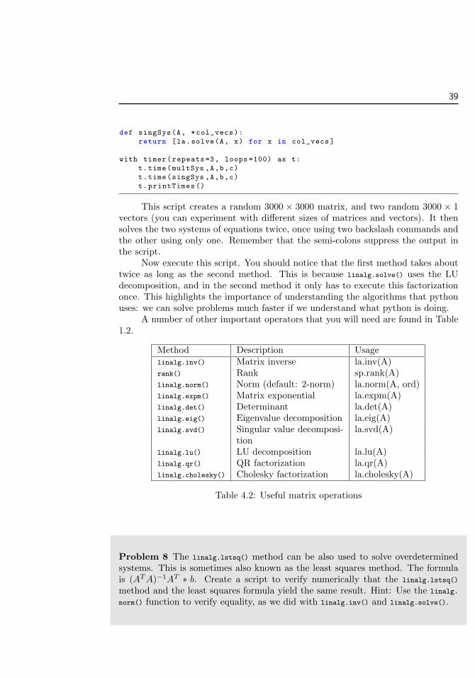
A number of other important operators that you will need are found in Table1.2.

Method Description Usagelinalg.inv() Matrix inverse la.inv(A)rank() Rank sp.rank(A)linalg.norm() Norm (default: 2-norm) la.norm(A, ord)linalg.expm() Matrix exponential la.expm(A)linalg.det() Determinant la.det(A)linalg.eig() Eigenvalue decomposition la.eig(A)linalg.svd() Singular value decomposi-

tionla.svd(A)

linalg.lu() LU decomposition la.lu(A)linalg.qr() QR factorization la.qr(A)linalg.cholesky() Cholesky factorization la.cholesky(A)

Table 4.2: Useful matrix operations

Problem 8 The linalg.lstsq() method can be also used to solve overdeterminedsystems. This is sometimes also known as the least squares method. The formulais (ATA)1AT b. Create a script to verify numerically that the linalg.lstsq()

method and the least squares formula yield the same result. Hint: Use the linalg.

norm() function to verify equality, as we did with linalg.inv() and linalg.solve().

Lab 5

Algorithms: MatrixOperations andAlgorithmic Complexity

Lesson Objective: This section explains how to create specific types of largematrices. It also introduces the concept of temporal complexity. Finally, it exploresSciPy’s special methods for working with sparse matrices.

Temporal ComplexityOne of the most important questions in scientific computing is: How long willthis operation take? The concept of temporal complexity attempts to answer thisquestion by determining how much time a function needs to operate on a given sizeof input. For example suppose calculating the inverse of a matrix of size n requiresthe following number of calculations.

f(n) =3n3

2+ 75n2 + 250n+ 30

What is the most important part of this expression? When our input gets verylarge the only relevant term in this equation is n3. For this reason we say thatf(n) 2 O(n3), or more commonly that f(n) is O(n3) (spoken “Big O of n cubed”or “Order of n cubed”). This notation is borrowed from analysis. This notationcaptures the salient behavior of our temporal complexity, or more precisely thegrowth rate we can expect of the execution time of our algorithm. We will discussthis concept later, but this is a simple introduction to the notion of complexityand Big O. Spatial complexity is the amount of memory an algorithm uses, and isdefined similarly.

Advanced Matrix ToolsWe now introduce a few di↵erent ways to build matrices. Two important methodsavailable for building matrices are zeros() and ones(). These commands allow us to

41

42 Lab 5. Matrices and Complexity

build matrices populated entirely with zeros or ones, respectively. For example, tobuild a 3-vector filled with zeros we enter the following command:

: import scipy as sp

: sp.zeros ((3 ,1))

array ([[ 0.],

[ 0.],

[ 0.]])

To find additional options for these methods, you can use the help system.One important use of the zeros() method is to allow us to pre-allocate memory.

Pre-allocation is simply the practice of reserving a chunk of memory for later use.We can always add more space to a matrix using the methods we learned in lab 1,but this requires many extra internal operations because of way arrays are storedin memory. Thus, it is generally faster to allocate a matrix with its final size andmodify its values rather than building an array as you go.

Table 1.3 gives a few commands that allow us to build types of useful matrices.

Function Description Usageeye() Identity matrix sp.eye(m, n)zeros() Zero matrix sp.zeros((m, n))ones() One matrix sp.ones((m, n))diag() Building (or retrieving)

along a diagonallinalg.toeplitz() Matrix with constant di-

agonalsla.toeplitz()

linalg.triu() Upper triangularlinalg.tril() Lower triangularrand Psuedo-random matrix,

uniformily distributedrandn Psuedo-random matrix,

normally distributedrandom.randint() Psuedo-random matrix,

uniformily distributedintegers

sp.random.randint()

tile() Copy across a given di-mension

sp.tile(A, reps)

Table 5.1: Special matrix creation commands

For example, suppose that we want to create a matrix with 2 on the diagonal,and ones on the super and sub diagonal. We can do this by using the followingcommand:


: la.toeplitz ([-2,1,0])

array([[-2, 1, 0],

[ 1, -2, 1],

43

[ 0, 1, -2]])

This matrix is useful because it numerically approximates the second deriva-tive of a function. We investigate some properties of this matrix in Problem 6 ofthis lab, and explain more about this matrix later.

Problem 1 Use the diagflat() method to create the following matrices. All of thesematrices should be easily scaleable (ie only minor modification would be requiredto change the size).

0

BBBB@

1 2 3 4 50 1 2 3 40 0 1 2 30 0 0 1 20 0 0 0 1

1

CCCCA

0

BBBB@

1 1/2 1/3 1/4 1/51/2 1 1/2 1/3 1/41/3 1/2 1 1/2 1/31/4 1/3 1/2 1 1/21/5 1/4 1/3 1/2 1

1

CCCCA

Problem 2 Create the matrices from Problem 1 using the methods linalg.toeplitz

() or linalg.triu(). Which method is easier? Now use whichever command is easiestto create the matrix: 0

BBBB@

1 0 0 0 00 2 0 0 00 0 3 0 00 0 0 4 00 0 0 0 5

1

CCCCA

Sparse MatricesIn this section we discuss how sparse matrices are used and constructed. A sparsematrix is a matrix that has few non-zero entries (where few is generally relative tothe number of entries in the matrix). SciPy has several di↵erent ways of storingsparse matrices. Each way has it pros and cons (the reader is encouraged to readthe help for way).

Type the following into IPython.

: from scipy import sparse as spar

: A = sp.diagflat ([2 ,3 ,4])

: B = spar.csc_matrix(A)

: C = B.todense ()

Notice that the matrix A has only three non-zero entries, and so we canconsider it sparse. In memory, an array stores a bit of data (be it an integer, float,


Function Descriptionsparse.bsr() Compressed Block Sparse Rowsparse.coo() Coordinatesparse.csc() Compressed Sparse Columnsparse.csr() Compress Sparse Rowsparse.dia() Sparse Diagonalsparse.dok() Dictionary of Keyssparse.lil() Linked List

Table 5.2: Sparse matrix representations in SciPy

or complex number) each entry, meaning that a 3 3 matrix requires a total 9blocks of memory. However, if we leverage the sparsity of A we realize that we onlyneed to store 3 numbers. The sparse methods do exactly this: they store only thenon-zero entries and their locations in the matrix. No longer are we working witharray. SciPy has many methods for performing operations on sparse arrays. Toconvert back to a dense matrix, we use the .todense() property of the sparse matrix.We can also convert between the di↵erent types sparse arrays.

We remark that if you want to make a sparse diagonal matrix, the best wayto do it isn’t to use diagflat() followed by sparse, it’s actually better to use thesparse.spdiags() method:

: spar.spdiags ([2,3,4],0,3,3)

This is because oftentimes when we are using sparse matrices we are dealingwith matrices that are too large to be handled eciently by python when representedin full form.

Banded MatricesA banded matrix is one whose only non-zero entries are diagonal strips. For exam-ple, the matrix

A =

0

BB@

1 2 0 03 4 5 00 6 7 80 0 9 10

1

CCA

is banded because there are three nonzero diagonals. This particular type of bandedmatrix is called a tri-diagonal matrix.

You can easily create banded matrices using the diagflat() method. For ex-ample, the matrix A above can be created by entering

: sp.diagflat ([3,6,9],-1) + sp.diagflat ([1,4,7,10],0) + sp.diagflat

([2,5,8],1)

45

Often a better way to create a tri-diagonal is it use the spar.spdiags() method.This is because many diagonal matrices are sparse. For example, we create thesame matrix in Python (while designating that it is sparse) using the command:

: Z = sp.array ([[3, 1, 0],[6, 4, 2],[9, 7, 5] ,[0 ,10 ,8]]).T

: spar.spdiags(Z,[-1,0,1],4,4)

For more information, check the documentation by typing spar.spdiags?. Forexample we create a tri-diagonal array with uniformily distributed random entries.This example also demonstartes the eciency of using sparse arrays.

: B = sp.rand (3 ,10000)

: A = spar.spdiags(B,range(-1,2) ,10000 ,10000)

: denseA = A.todense () #only do this step if you have _lots_ of

memory!

: A.data.nbytes

240000 #about 0.24 MB of memory

: denseA.nbytes

800000000 #about 762.9 MB of memory!

We can’t use the full command in this case because the computer will almostcertainly run out of memory (the matrix is 10,000 10,000). However, we can stillvisualize this matrix using the plt.spy() command from matplotlib, which essentiallyshows the location of non-zero entries in a matrix. The output of plt.spy(A) in thiscase is shown in Figure 1.2:

Figure 5.1: The output of the spy command.


Using Sparse MatricesConsider the linear system Ax = b, where A is a 100,000 100,000 tri-diagonalmatrix. To store a full matrix of that size in your computer, it would normallyrequire 10 billion double-precision floating-point numbers. Since it takes 8 bytesto store a double, it would take roughly 80GB to store the full matrix. For mostdesktop computers, that fact alone makes the system numerically prohibitive tosolve. The temporal complexity of the problem is even more problematic. Methodsfor directly solving an arbitrary linear system are usually O(n3). As a result, evenif the computer could store an 80GB matrix in RAM, it would still take severalweeks to solve the system. However, since we don’t have computers with that muchavailable RAM, most of the matrix would have to be stored on the hard drive, sothe computation would probably take between 6 months to a year.

The point is that even the next generation of computers will struggle withsolving arbitrary linear systems of this size in a reasonable period of time. However,if we take advantage of the sparse structure of the tri-diagonal matrix, we can solvethe linear system, even with a modest modern computer. This is because all ofthose zeros don’t need to be stored and we don’t need to do as many operations torow reduce the tri-diagonal system.

Let’s first compute the spatial complexity of the above system when consideredas a sparse matrix. There are three diagonals that have roughly 100,000 non-zeroentries. That’s 300,000 double-precision floating point numbers, which is about 2.4MB (Less storage than your favorite song). As a result, it will easily fit into thecomputer’s RAM. Furthermore, the temporal complexity for solving a tri-diagonalmatrix is O(n). Let’s see how long it takes to solve the system for random data:

: from scipy.sparse import linalg as sparla

: from timer import timer

: D = sp.rand(3, 100000)

: b = sp.rand(1, 100000)

: A = spar.spdiags(D,[ -1 ,0 ,1] ,100000 ,100000)

: def solSys ():

....: return sparla.spsolve(A,b)

: with timer() as t:

....: t.time(solSys)

....: t.printTimes ()

Problem 3 Write a function that returns a full n n tri-diagonal array with 2’salong the diagonal and 1’s along the two sub-diagonals above and below the di-agonal. Hint: Use the la.toeplitz() method. Note that this is the second derivativematrix that we discussed at the beginning of this lab.

Problem 4 Write another function that builds the same array as above, but as a

47

sparse array. You must build this as a sparse matrix from the beginning. Hint: Usethe spar.spdiags() method.

Problem 5 Solve the linear system Ax = b where A is the nn tri-diagonal arrayfrom the above two problems and b is randomly generated. How high can you gofor each method? Make a table for several di↵erent values of n and the time it tookto solve for each run. What conclusions can you draw?

Problem 6 Using the sparse array above and the method la.eigs(), calculate thesmallest eigenvalue of the array as the array’s size goes to infinity. What valuedoes n2 approach? Hint: It’s the square of an important number. This is relatedto operator theory: the second derivative operator has this eigenvalue in certaincases.

Other Sparse CommandsOne important method of sparse array objects is the nonzero() method, which isrelated to the number of nonzero entries in an array. This number is importantbecause it is an indicator of the amount of time and space that is required tooperate on the sparse array. You should be aware that there is some overhead tousing and storing the sparse array data structure. Sparsely represented arrays arevery beneficial when the number of nonzero entries is relatively small compared tothe total number of entries. When the array has many nonzero entries, a sparserepresentation becomes disadvantageous. To see this, create and execute a scriptwith the following code:

: A = sp.rand (600 ,600); B = spar.csc_matrix(A)

: def square(A): return sp.power(A, 2)

: with timer() as t:

....: t.time(square , A)

....: t.time(square , B)

Run the script and note the two di↵erent runtimes. Notice that it takes muchlonger to square the sparse array. This is because the sparse array data structure isoptimized for arrays that are actually sparse. The array A is entirely nonzero. Thus,you incur the overhead of the sparse array representation without any benefits sincethere are no entries you are not required to store or compute. To summarize, onlyuse a sparse array when your array is in fact sparse. Using sparse arrays for mostlynonzero arrays will negatively impact performance and memory requirements.


Just as with dense arrays, we can pre-allocate sparse arrays. Sometimes it isnecessary to create sparse matrices that do not have a nice banded pattern. Weinitialize a sparse array just like any other array. The most ecient sparse array forpre-allocation is LIL. Once you are done constructing you sparse array and wish toperform calculations, you should convert to a more ecient sparse array (CSR orCSC).

: Z = spar.lil_matrix ((400 ,300))

<400x300 sparse matrix of type ’<type ’numpy.float64 ’>’

with 0 stored elements in LInked List format >

: Z[1 ,34] = 23

: Z[23 ,32] = 56

: Z[2,:] = 13.2

This code snippet creates a 400 300 LIL sparse array. We can then workwith the sparse array as though it were a dense array. When the array is initializedall of the entries are assumed to be zero.

Lab 6

Applications: MarkovChains I

Lesson Objective: This section teaches about two simple applications of LinearAlgebra. First it teaches about Markov Chains, which in this context representdiscrete random transitions. Second it teaches about Graph Theory, which can beused to represent many physical problems.

Markov ChainsAMarkov Chain describe a particular type of random variable. This type of randomvariable is characterized by the fact that all relevant information is related to itscurrent state. We can easily model this type of random variable using matrices. Wewill start with a canonical example of a frog jumping from one lilypad to another.

Fredo the Frog hops around between the three lily pads A, B, and C. If he’son lily pad A and jumps, there is a 25% chance that he will land back on lily padA, a 25% chance that he will land on lily pad B, and a 50% chance that he willland on lily pad C. In Figure ‘2.1, we have a transition diagram that reflects thevarious probabilities from which Fredo will go from one lily pad to another.

We can convert our transition diagram into a transition matrix, where the(i, j)-entry of the matrix corresponds to the probability that Fredo jumps from thejth lily pad to the ith lily pad (where of course A is the first lily pad, B is thesecond, and so on). In Fredo’s case, the transition matrix is

A =

0

@1/4 1/2 1/21/4 1/6 1/21/2 1/3 0

1

A

Note that all of the columns add up to one. This is important.If Fredo is on lily pad A, where will he be after two jumps? By multiplying

the matrix A by itself, we have (approximately)

49

50 Lab 6. Markov Chains I

Figure 6.1: Transition diagram for Fredo the Frog

A2 =

0

@0.4375 0.3750 0.37500.3542 0.3194 0.20830.2083 0.3056 0.4167

1

A

From this, we infer that there is a 43.75% chance he will still be on lily pad Aafter two jumps. Note that he might have jumped from A to A to A, denotedA ! A ! A, or he could have jumped to one of the other lily pads and then backagain, that is, either A ! B ! A or A ! C ! A. In addition, there is a 35.42%chance he will be on lily pad B and a 20.83% chance that he will be on lily pad C.Using Python, we can type in our transition matrix and see where Fredo will beafter 5, 10, 20 or 100 jumps.

#Remember , the 1.’s in the numerator force floating point division

: A = sp.array ([[1./4 ,1./2 ,1./2] ,[1./4 ,1./6 ,1./2] ,[1./2 ,1./3 ,0]])

: np.linalg.matrix_power(A,5)




Note that in the limit that the number of jumps goes to infinity, we get

A1 =

0

@0.4 0.4 0.40.3 0.3 0.30.3 0.3 0.3

1

A

This means that after several jumps, the probability that we will find Fredo on agiven lily pad will have nothing to do with where he started initially.

51

Markov ChainsWe can generalize this notion beyond that of frogs and lily pads. Let the state ofour system be represented by a probability vector

x =

2

6664

x1

x2...xn

3

7775

where each entry represents the probability of being in that state. Note that eachentry is nonnegative and the sum of all the entries adds up to one. For example,in the case of Fredo, if we know initially that he is on lily pad A, then we have thestate vector

x0 =

2

4100

3

5

because we know for certainty (100%) that Fredo is in the first state. After onejump, we have

x1 = Ax0 =

2

40.250.250.50

3

5

After two jumps, we have

x2 = Ax1 = A2x0 =

2

40.43750.35420.2083

3

5

After a large number of jumps (n >> 1), we have

xn = Axn1 = · · · = Anx0

2

40.40.30.3

3

5

Since all of the columns are the same for A1, then for any initial probability vectorx0, we get the same limiting output, or in other words, all initial vectors convergeto the same point, call it x1. Moreover, we have that

x1 = Ax1

This is called a stable fixed point. How can we check that a stable fixed pointexists? Hint: Think eigenvalues and eigenvectors.

ExampleConsider the Markov chain given by

A =

0

@0.5 0.3 0.40.2 0.2 0.30.3 0.5 0.3

1

A .


We show that it has a stable fixed point by checking that it has a single eigenvalue = 1. We do this via Python:

: A = sp.array ([[.5 ,.3 ,.4] ,[.2 ,.2 ,.3] ,[.3 ,.5 ,.3]])

: V = la.eig(A)[1]

Note that the entries in the = 1 eigenvector do not generally add up to one.Indeed, any multiple of an eigenvector is an eigenvector. So we need to multiply itby the appropriate constant so that all of the entries add up to one.

: x = V[:,0]

: x = x/sp.sum(x);x

array([ 0.41836735 , 0.23469388 , 0.34693878])

We can check this answer by taking A to a high exponent, say A100.

Problem 1 Suppose a basketball player’s success at shooting free throws can bedescribed with the following Markov chain

A =

.75 .50.25 .50

where the first state corresponds to success and the second state to failure.

1. If the player makes his first free throw, what is the probability that he alsomakes his third one?

2. What is the player’s average free throw percentage?

Problem 2 Consider the Markov process given by the transition diagram in Figure2 below:

1. Find the transition matrix.

2. If the Markov process is in state A, initially, find the probability that it is instate B after 2 periods.

3. Find the stable fixed point if it exists.

53

Figure 6.2: Transition diagram

Graph Theory

Graph theory is an important branch of mathematics and computer science.It describes how objects are connected to one another. In a rigorous sense, a graphis composed of two sets: a set of nodes and a set of edges that connect these nodes.

A graph is directed if connections are uni-directional, and undirected if theyare bi-directional. The above graphic shows an undirected graph. We can write amatrix that describes this type of graph. We let each row of our matrix representour starting point and each column represent our destination. We put a 1 if thereis a path and a 0 if there is not. For the above graph we generate the followingmatrix:

A =

0

BBBBBB@

0 1 0 0 1 01 0 1 0 1 00 1 0 1 0 00 0 1 0 1 11 1 0 1 0 00 0 0 1 0 0

1

CCCCCCA


This matrix is called an adjacency matrix. Note that this matrix is symmetric,since the graph is undirected.

What happens if we square an adjacency matrix? It turns out that raising anadjacency matrix to the n power yields the number of paths of length n betweentwo vertices. For example by squaring the above matrix Python gives:


array ([[2, 1, 1, 1, 1, 0],

[1, 3, 0, 2, 1, 0],

[1, 0, 2, 0, 2, 1],

[1, 2, 0, 3, 0, 0],

[1, 1, 2, 0, 3, 1],

[0, 0, 1, 0, 1, 1]])

Now try to find the number of connections of length 6 from node 3 to itself.This is simple to do in Python:


array ([[45, 54, 38, 45, 54, 16],

[54, 86, 29, 77, 51, 11],

[38, 29, 55, 15, 70, 27],

[45, 77, 15, 75, 31, 4],

[54, 51, 70, 31, 93, 34],

[16, 11, 27, 4, 34, 14]])

It turns out that there are 55 unique paths of length 6 from node 3 to itself. Imaginetrying to count all of those paths by hand! It would be very easy to count incorrectly.However, this method makes it very simple to count paths without any mistakes.

Problem 3 Let the following matrix represent a directed graph

A =

0

BBBBBBBB@

0 0 1 0 1 0 11 0 0 0 0 1 00 0 0 0 0 1 01 0 0 0 1 0 00 0 0 1 0 0 00 0 1 0 0 0 10 1 0 0 0 0 0

1

CCCCCCCCA

The greatest number of paths of length five are from which node to each node?From which node to which node is their no path of length seven?

The astute reader may ask now why this matters. It turns out that thestudy of graphs and connectivity have many important applications. For example,connections between web pages can be described as graphs. So can flights betweenairports or friends on social networking sites. The same ideas are applied frequentlyin computer chip design and in the preservation of endangered species. We willexplore one surprising application to chemistry.

55

Remeber the bucky array we explored in chapter one? The graph that thismatrix represents is a graph for a geodesic dome, which has structure almost iden-tical to certain types of carbon atoms. Understanding the graphs of certain typesof molecules allows scientists to better understand the structure of the molecule,making identification and manipulation easier.

We will manipulate the matrix the bucky to simulate the types of analysis ascientist could do on a complex carbon atom. For our purposes, each column androw of the bucky matrix represents an atom in our molecule, and connections arechemical bonds from one atom to another.

Problem 4 Find the number of connections between atoms in our molecule(thecommand sp.count_nonzero may be useful). Then find the number of atoms thatare connected by paths of length two. Three? At what path length are all of theatoms connected? A nifty way to visualize this is the plt.spy command. Readthe documentation for plt.spy and then use plt.spy to visualize how the graph isconnected at path length one, two, four and ten. Remember, to load ‘‘bucky.csv’’

into an array use the command bucky = sp.loadtxt ( "bucky.csv", delimiter = ",").

Lab 7

Algorithms:RREF/ElementaryMatrices

Lesson Objective: In this section we will use elementary matrices to find theRREF and to find the LU decomposition.

In Linear algebra there are 3 elementary row operations: switching two rows,multiplying a row by a constant, and adding a multiple of one row to another row.We carry out each of these operations with a corresponding elementary matrix.These matrices are easy to construct. Suppose A is an m n matrix and youwant to perform one of the three elementary operations on A. You can do this beconstructing the mm identity matrix, I, performing the elementary row operationon I to obtain E and then multiplying EA. For example, consider the matrix

A =

0

@a11 a12 a13 a14a21 a22 a23 a24a31 a32 a33 a34

1

A

If we want to swap the first two rows, we can left multiply the matrix A by:

E =

0

@0 1 01 0 00 0 1

1

A ,

then

EA =

0

@a21 a22 a23 a24a11 a12 a13 a14a31 a32 a33 a34

1

A .

E in this case is called a type I matrix.Now let’s examine the next row operation. If we want to multiply, say, the

second row of A by the constant b, we can left multiply the matrix A by the following

57

58 Lab 7. RREF/Elementary Matrices

matrix:

E =

0

@1 0 00 b 00 0 1

1

A .

Then

EA =

0

@a11 a12 a13 a14ba21 ba22 ba23 ba24a31 a32 a33 a34

1

A .

E is called a type II matrix.Now let’s examine the last row operation. If we want to multiply, say, the first

row of A by a constant c and add it to the second row, we can left multiply thematrix A by the following matrix:

bE =

0

@1 0 0c 1 00 0 1

1

A .

Then

bEA =

0

@a11 a12 a13 a14

ca11 + a21 ca12 + a22 ca13 + a23 ca14 + a24a31 a32 a33 a34

1

A .

bE is called a type III matrix.Below, the elementary matrices corresponding to each row operation is imple-

mented in Python.

1 from scipy import eye

2

def rowswap(n, j, k):

4 """ Swaps two rows

6 INPUTS: n -> matrix size

j, k -> the two rows to swap """

8 out = eye(n)

out[j,j]=0

10 out[k,k]=0

out[j,k]=1

12 out[k,j]=1

return out

14

def cmult(n, j, const):

16 """ Multiplies a row by a constant

18 INPUTS: n -> array size

j -> row

20 const -> constant """

out = eye(n)

22 out[j,j]= const

return out

24

def cmultadd(n, j, k, const):

26 """ Multiplies a row (k) by a constant and adds the result to

another row (j)"""

59

out = eye(n)

28 out[j,k] = const

return out

row opers.py

Programming Row ReductionA fundamental problem in linear algebra is using matrix representations to solvesystems of linear equations. In this section, we do this by using elementary matricesto reduce a matrix into “row echelon form” (REF), as opposed to “reduced rowechelon form” (RREF). We remark that to solve a linear system, it is actuallyfaster computationally to use REF and then finish with back-substitution, than itis to use RREF. Consider the following matrix:

0

@4 5 6 32 4 6 47 8 0 5

1

A

By iteratively left multiplying by elementary matrices, we can reduce as fol-lows:

Remember that our functions returns the elementary array corresponding tothe desired row operation. Also note that setting the type of our initial array iscrucial.

: import scipy as sp

: import row_opers as op

: A = sp.array ([[4, 5, 6, 3],[2, 4, 6, 4],[7, 8, 0, 5]], dtype=’

float32 ’)

array ([[ 4., 5., 6., 3.],

[ 2., 4., 6., 4.],

[ 7., 8., 0., 5.]], dtype=float32)

: A1 = sp.dot(op.cmultadd (3,1,0,-A[1 ,0]/A[0 ,0]), A); A1

array ([[ 4. , 5. , 6. , 3. ],

[ 0. , 1.5, 3. , 2.5],

[ 7. , 8. , 0. , 5. ]])

: A2 = sp.dot(op.cmultadd (3,2,0,-A1[2 ,0]/A1[0 ,0]), A1); A2

array ([[ 4. , 5. , 6. , 3. ],

[ 0. , 1.5 , 3. , 2.5 ],

[ 0. , -0.75, -10.5 , -0.25]])

: A3 = sp.dot(op.cmultadd (3,2,1,-A2[2 ,1]/A2[1 ,1]), A2); A3

array ([[ 4. , 5. , 6. , 3. ],

[ 0. , 1.5, 3. , 2.5],

[ 0. , 0. , -9. , 1. ]])

To complete REF we would need to divide each row by its leading coecient.We can do that using Type II matrices. We leave it to you to carry this out.

60 Lab 7. RREF/Elementary Matrices

Problem 1 Write a Python function, which takes as input an n(n+1) matrix (inother words and augmented matrix) and performs the above naive row reduction toREF using elementary matrices. (You do not need to worry about underdeterminedmatrices or getting zeros on the main diagonal)

LU DecompositionAgain, consider the matrix A. By iteratively left multiplying by Type 3 elementarymatrices, we reduce as follows:

: E1 = op.cmultadd (3,1,0,-A[1 ,0]/A[0 ,0]); E1

array ([[ 1. , 0. , 0. ],

[-0.5, 1. , 0. ],

[ 0. , 0. , 1. ]])

: B1 = sp.dot(E1, A)

array ([[ 4. , 5. , 6. , 3. ],

[ 0. , 1.5, 3. , 2.5],

[ 7. , 8. , 0. , 5. ]])

: E2 = op.cmultadd (3,2,0,-B1[2 ,0]/B1[0 ,0])

: B2 = sp.dot(E2, B1)

: E3 = op.cmultadd (3,2,1,-B2[2 ,1]/B2[1 ,1])

: U = sp.dot(E3, B2); U

array ([[ 4. , 5. , 6. , 3. ],

[ 0. , 1.5, 3. , 2.5],

[ 0. , 0. , -9. , 1. ]])

Note that we have reduced the above matrix into upper-triangular form, denotedas U . Hence, we have

U = E3E2E1A.

Since the elementary matrices are invertible, we also have

(E3E2E1)1U = A.

This can be re-written asE1

1 E12 E1

3 U = A.

Then we define L to beL = E1

1 E12 E1

3 ,

which yields LU = A.


: I = lambda x: la.inv(x)

: L = sp.dot(sp.dot(I(E1), I(E2)), I(E3)); L

array ([[ 1. , 0. , 0. ],

[ 0.5 , 1. , 0. ],

[ 1.75, -0.5 , 1. ]])

: sp.dot(L, U)

array ([[ 4., 5., 6., 3.],

[ 2., 4., 6., 4.],

[ 7., 8., 0., 5.]])

61

What makes LU decomposition so easy is that the inverses of elementary matricesare elementary matrices. For example, the inverse of a Type 3 elementary matrixis the same matrix with the opposite sign in the (j, k) entry. In the above problem,we have: Note that the minus signs are gone. Doing it this way, we don’t have toactually invert anything to compute L. This makes the computation much faster.

Why Should I Care?The LU Decomposition isn’t very useful when doing matrix computation by hand.It is, however, very important in scientific computation for the following reasons:

• If you want to solve the matrix equation Ax = b, for several di↵erent b0s,you can replace A with L and U , giving LUx = b. Then solve the equationsLy = b and Ux = y, using forward and backward substitution, respectively.This is actually faster than solving them with row reduction.

• The LU decomposition allows quick computation of both inverses and deter-minants.

• For very large matrices the LU decomposition is crucial. Indeed one canperform the LU decomposition on a given matrixA without needing additionalspace, that is, the program actually over-writes A with L and U . Note thatsince the diagonal of L are all ones, they don’t need to be stored, and sothe upper diagonal (including the diagonal) is U and the lower diagonal (notincluding the diagonal) is L.

Problem 2 Write a Python function which takes as input a random nn matrix,performs the LU decomposition and returns L and U . To verify that it works,multiply L and U together and compare to A. Note: you should not use the inv

function when you do this. You should only use the elementary matrices thatwe just created. Additionally, have your function count the number of operationsneeded to perform the LU decomposition.

Problem 3 Write a Python function which uses the solution to Problem 2 to findthe determinant of A.

Applied Mathematics - GitHub Pagessethc23.github.io/wiki/Python/good_python_intro.pdfto other topics...

Documents

Transcript of Applied Mathematics - GitHub Pagessethc23.github.io/wiki/Python/good_python_intro.pdfto other topics...