Applied Brief Notes Mechanics - California Institute of...

cs butxceedlineto

uld be

Three

nthstension

Journal ofApplied

Mechanics Brief NotesA Brief Note is a short paper that presents a specific solution of technical interest in mechaniwhich does not necessarily contain new general methods or results. A Brief Note should not e1500 wordsor equivalent~a typical one-column figure or table is equivalent to 250 words; a oneequation to 30 words!. Brief Notes will be subject to the usual review procedures priorpublication. After approval such Notes will be published as soon as possible. The Notes shosubmitted to the Technical Editor of the JOURNAL OF APPLIED MECHANICS. Discussions on the BriefNotes should be addressed to the Editorial Department, ASME, United Engineering Center,Park Avenue, New York, NY 10016-5990, or to the Technical Editor of the JOURNAL OF APPLIEDMECHANICS. Discussions on Brief Notes appearing in this issue will be accepted until two moafter publication. Readers who need more time to prepare a Discussion should request an exof the deadline from the Editorial Department.

t

ara

n

ento-

pos-m-

edent-

e de-

ssssti-

-

n

On the Relation Between theL-Integral and the BuecknerWork-Conjugate Integral

J. P. Shi, X. H. Liu, and J. M. LiDepartment of Engineering Mechanics, Xi’an Universityof Technology, 710048 Xi’an, China

A simple but inherent relation between the L-integral andBueckner work conjugate integral is deduced for crack problemisotropic, anisotropic, and dissimilar materials, respectively. Itproved the L-integral, from the mathematical point of view as was in principle, is arising from the Betti’s reciprocal theorem.@S0021-8936~00!00103-3#

1 IntroductionKnowles and Sternberg@1# have shown that theL-integral is

given by

L5 RGe3i j ~Wxjni2Tiuj2Tkuk,ixj !ds (1)

whereG is a closed contour in thex15x, x25y plane surroundinga whole crack;W is the strain energy density, andTi is the tractionacting on the outer side of theG. The characteristics of theL-integral and theJk-integral are different. It can be proven ththe L-integral is a path-independent integral. We can also vethat theL-integral is independent of the selection of the coordinsystem.

The Bueckner work-conjugate integral~@2#! was derived fromthe well-known Betti’s reciprocal theorem, which could be formlated as follows:

I G5EG~ui

~ I !s i j~ II !2ui

~ II !s i j~ I !!njds ~ i , j 5x,y! (2)

where the superscripts~I! and ~II ! refer to two possibledisplacement-stress fields which satisfy the traction-free co

Contributed by the Applied Mechanics Division of THE AMERICAN SOCIETY OFMECHANICAL ENGINEERS for publication in the ASME JOURNAL OF APPLIEDMECHANICS. Manuscript received by the ASME Applied Mechanics Division, Ju6, 1999; final revision, January 21, 2000. Associate Technical Editor: J. T. Ju.

828 Õ Vol. 67, DECEMBER 2000 Copyright ©

hein

isell

tifyte

u-

di-

tions on the crack faces. The property of the path-independintegral is proved by Bueckner using Betti’s work reciprocal therem, that isI G5I C .

2 ProofFor homogeneous isotropic materials, assume that the first

sible displacement-stress field is induced by the following coplex potentialsw(z) andc(z):

w8~z!51

Az22a2 (k51

1`

Ekzk1(

k51

1`

Fkzk21

(3)

c8~z!51

Az22a2 (k51

1`

Ekzk2(

k51

1`

Fkzk21

whereEk and Fk are complex coefficients which can be definby remote conditions. Introduce a supplemental displacemstress field defined by the following complex potentialsw (II )(z)andc (II )(z):

w~ II !~z!52 izw8~z!(4)

c~ II !~z!52 izc8~z!12i zw8~z!.

The corresponding displacement and stress components arrived as follows:

ui~ II !5yui ,x2xui ,y

s i j~ II !5ys i j ,x2xs i j ,y1

1

2E s i j ,xdy21

2E s i j ,ydx ~ i , j 51,2!

(5)

whereui ands i j , as the~I! field, are the displacement and strecomponents induced by Eq.~3!. It can be examined that the stress i j

~II ! satisfy the traction-free conditions on the crack faces. Subtuting Eq.~5! andui ands i j into Eq. ~2!, we obtain

I G5E Fuis i j ,xy2uis i j ,yx2ui ,xs i j y1ui ,ys i j x

11

2uiE s i j ,xdy2

1

2uiE s i j ,ydxGnjds (6)

wheredx52n2ds, dy5n1ds.Now, theI G – 2L is examined. Utilizing the equilibrium condi

tions in plane problems and noting the integral termsTiui , s i j uiand ui*s i j ,xdy have no contribution forI G22L when r→0 ~atthe near of crack tip!. Thus,I G – 2L is equal to zero. We obtaine

2000 by ASME Transactions of the ASME

rh

e

d

t

-

in

o

i

l

s

rom

thealllexare

c-nderrilla-

t in

’sate

hersub-ath-

s in

o-

ce

ch.

a,

ede-

lyr.

I G52L. (7)

Equation~7! shows that between theL-integral and the Buecknework conjugate integral there is a simple but inherent relationsWe need not to know the obvious function expressions of coplex potentials for the crack beforehand, but the traction-free cditions must be satisfied.

If there are two displacement-stress fields, namely,ui , s i j andui

(II ), s i j(II ), using the Betti’s reciprocal theorem to the regio

bounded by crack borders, one can divide the contourC into CL ,CR andC1 ,C2 , whereCL ,CR are circles around the left and thright crack tips andC1 ,C2 are the straight line along the uppeand lower crack faces, respectively. Because the stresses aron the crack faces, thenI G5I CL1I CR . In this case, if integralsI CL andI CR can be evaluated for some displacement-stress fiethen the path-independent integralI G can also be defined anevaluated. If the displacement-stress fields are defined by Eqs~3!and ~4!, we can deduce the following relationship betweenL-integral and the stress intensity factors:

L523~k21!a

4m~K1LK2L1K1RK2R! (8)

whereKL5K1L1 iK 2L , KR5K1R1 iK 2R are stress intensity factors at the left and the right crack tips, respectively.k andm areelastic constants.

3 DiscussionThe complex potentials of the center crack,w1(z),v1(z),

w2(z),v2(z), were obtained by Chen and Shi@3# by using thesame method obtained the eigenfunction expansion form by R@4# in interfacial cracks for dissimilar material. The stress adisplacement fields that are obtained from these complex potials satisfy the traction-free conditions on the crack faces andcontinuous condition along the entire interface.

A supplemental displacement-stress field defined bycomplex potentials w1

(II )(z),v1(II )(z),w2

(II )(z),v2(II ) is intro-

duced. The relations betweenw1(II )(z),v1

(II )(z),w2(II )(z),v2

(II )

andw1(z),v1(z),w2(z),v2(z) are analogous to Eq.~4!.In a similar manner, the displacement and stress of the~II ! field

are presented in Eq.~5!. They satisfy the traction-free conditionon the crack faces also. The corresponding displacementstress components will be substituted into Eq.~6!. Note that thecurveG can be divided into two sections: curveG1 of the upperplane and the curveG2 of the below plane. The deductions of Eq~6! to ~7! relate to the equilibrium equations in plane problemand traction-free conditions only, but don’t involve the materparameter. The process is the same as the above homogeisotropic material. Finally, we still obtain Eq.~7! in the interfacecrack, that isI G52L.

BetweenL-integral and stress intensity factors there is the flowing relation:

L52S k121

m11

k221

m2D 3~K1LK2L1K1RK2R!

8 cosh2~p«!a (9)

where « is ‘‘oscillation index’’ and KL5K1L1 iK 2L , KR5K1R1 iK 2R are complex stress intensity factors at the left and the rcrack-tips, respectively. They cannot be separated into the pumodel and II model;k1 ,m1 and k2 ,m2 stand for the materiaparameters of the upper and lower plane.

For anisotropy material, the Lekhenitski complex potenttheory needs to be used~@5#!. According to the need of the Bueckner work conjugate integral, the subsidiary stress-displacemfields, which represents~II ! field, are

w~ II !~z1!52 iz1w8~z1!

c~ II !~z2!52 iz2c8~z2!12i z2w8~z1!. (10)

Copyright © 2Journal of Applied Mechanics

ip.m-on-

n

erfree

lds,

.he

icendten-the

the

sand

s.s

aleous

l-

ghtre I

ial-ent

The stress fields caused by Eq.~10! satisfy the traction-freeconditions. The relation between the~II ! field and a physical stresfield are analogous to Eq.~5!.

By proceeding in the same manner as the isotropic case fEq. ~6! to Eq. ~7!, we draw a conclusionI G52L.

It can be seen that a simple but inherent relation betweenL-integral and the Bueckner work conjugate integral is rightalong, although the characteristic of material is more compthan isotropic and the complex potentials in these two casesmore different with in isotropic.

4 ConclusionsUsing the Bueckner work conjugate integral through introdu

ing a special subsidiary stress-displacement field, one can rethe L-integral. The relation betweenL-integral and the Buecknework conjugate integral seems independent of the stress osctory singularities on the interface crack tips and the eigenroothe anisotropy. It is found that theL-integral, from the mathemati-cal point of view as well as in principle, is arising from the Bettireciprocal theorem. This means that the Bueckner work conjugintegral is a more general path-independent integral than otare. Using the Bueckner integral through choosing a different ssidiary stress-displacement field could render any other pindependent integrals.

References@1# Knowles, J. K., and Sternberg, E., 1972, ‘‘On a Class of Conservation Law

Linearized and Finite Elastostatics,’’ Arch. Ration. Mech. Anal.,44, pp. 187–211.

@2# Bueckner, H. F., 1973,Mechanics of Fracture: Methods of Analysis and Slution of Crack Problems, G. C. Sih, ed., Noordhoff, Leyden, pp. 239–314.

@3# Chen, Y. H., and Shi, J. P., 1998, ‘‘On the Relation Between theM-integraland the Bueckner Work-Conjugate Integral,’’ Acta Mech. Sin.,30, pp. 495–502 ~in Chinese!.

@4# Rice, J. R., 1988, ‘‘Elastic Fracture Mechanics Concepts for InterfaCracks,’’ J. Appl. Mech.,55, pp. 98–103.

@5# Sih, G. C., and Chen, E. P., 1981, ‘‘Cracks in Composite Materials,’’ MeFracture,6, pp. 1–99.

A Note on the Driving Traction Actingon a Propagating Interface:Adiabatic and Non-Adiabatic Processesof a Continuum

R. AbeyaratneMem. ASME, Department of Mechanical Engineering,Massachusetts Institute of Technology, Cambridge,MA 02139

J. K. KnowlesFellow ASME, Division of Engineering and AppliedSciences, California Institute of Technology, PasadenCA 91125

An expression for the driving traction on an interface is derivfor an arbitrary continuum undergoing an arbitrary thermomchanical process which may or may not be adiabatic.@S0021-8936~00!00403-7#

Contributed by the Applied Mechanics Division of THE AMERICAN SOCIETY OFMECHANICAL ENGINEERS for publication in the ASME JOURNAL OF APPLIEDMECHANICS. Manuscript received by the ASME Applied Mechanics Division, Ju30, 1997; final revision, Aug. 5, 1997. Associate Technical Editor: L. T. Wheele

000 by ASME DECEMBER 2000, Vol. 67 Õ 829

,n

c

ax

e

r

i

in

e

n

w

, forace-to

ely.es

ust

va--ith

heov-to

1 SummaryIn this note we derive an expression for the ‘‘driving traction

or Eshelby force~@1#!, acting on a propagating interface in a cotinuum. The interfaces that we have in mind might represent,example, a shock wave or a boundary between two phasesmaterial, and the thermomechanical processes which thetinuum is permitted to undergo may or may not be adiabatic. Frthe perspective of irreversible thermodynamics, the driving trtion corresponds to a ‘‘thermodynamic affinity’’; see, for eample,@2–4#. It plays a central role in modeling the kinetics ophase transformations by characterizing the rate of propagatiophase boundaries~e.g., see@5–8#!.

The derivation sketched below makes no assumptions abouconstitutive law for the continuum under consideration. Whspecialized to a thermoelastic material, the expression for the ding traction obtained here has certain similarities with the Lendre transform of the Helmholtz free-energyc~F,u! with respectto both the deformation gradient tensorF and the temperatureu,as well as with the Legendre transform of the internal ene«~F,h! with respect toF and the specific entropyh.

The result derived here generalizes an earlier one whichbeen established for non-adiabatic processes~@9,10,5#!. Thisformer characterization of driving traction was not valid in adbatic processes, and therefore did not, in particular, apply to shwaves in classical gas dynamics or to impact-induced rapmoving phase boundaries in solids. A one-dimensional versiothe present result was obtained in@11#.

2 Momentum and EnergyConsider a body which occupies a regionR in a reference con-

figuration. LetxPR denote the position of a particle in this configuration and lett denote time. Consider a thermomechanicprocess of this body on some time interval@ t1 ,t2# which is char-acterized by the motiony(x,t), body force per unit massb(x,t),Piola-Kirchhoff stresss(x,t), heat fluxq(x,t), heat supplyr (x,t)and internal energy per unit mass«(x,t). Suppose that during thisprocessy is continuous with piecewise continuous first and sond derivatives onR3@ t1 ,t2#; b(•,t) and r (•,t) are continuouson R; s(•,t) andq(•,t) are piecewise continuous with piecewiscontinuous gradient onR; and « is piecewise continuous withpiecewise continuous first derivatives onR3@ t1 ,t2#. During thisprocess, the usual balance laws of linear and angular momenand the first law of thermodynamics require that for any subregD,

E]D

sn dA1EDrb dV5

d

dt EDrv dV, (1)

E]D

y3sn dA1EDy3rb dV5

d

dt EDy3rv dV, (2)

E]D

~sn•v1q•n!dA1ED~rb•v1rr !dV

5d

dt EDS 1

2rv•v1r« DdV. (3)

Herev5y denotes particle velocity,r~x! is the mass density in thereference configuration which is assumed to be continuous oR,andn is a unit outward normal vector on]D.

At a point inR at which the fields are smooth the balance la~1!–~3! yield the usual field equations

Div s1rb5r v, (4)

sFT5FsT, (5)

s•F1Div q1rr 5r«, (6)

whereF5Grady is the deformation gradient tensor.

830 Õ Vol. 67, DECEMBER 2000

’’-forof aon-

omc--fn of

t theenriv-g-

gy

had

a-ockdly

of

-al

c-

e

tumion

s

Next, suppose that there is a surfaceSt in R such that the fieldsF, v, q, s and« suffer jump discontinuities acrossSt while beingcontinuous on either side of it. Such a surface may representexample, the Lagrangian image of a shock wave or an interfseparating two material phases. LetVn>0 denote the normal velocity of propagation of this interface. We refer to the side inwhich Vn points as the positive side ofSt . For any field quantity

g(x,t) let g1 and g2 denote the limiting values ofg as a point onSt is approached from its positive and negative side, respectivThen, we let@@g## and^g& denote the jump and the average valuof g on St :

@@g##5 g12 g2, ^g&51

2~ g11 g2 !. (7)

At a point onSt , the balance laws~1!–~3! yield the usual jumpconditions

@@sn##1@@rv##Vn50, (8)

@@sn•v##1F Fr«11

2rv•vG GVn1@@q•n##50. (9)

The energy jump condition~9! can be written in the followingalternative form by making use of~8! and @@v##1Vn@@Fn##50which follows from the continuity of the deformation~for alge-braic details see, for example,@5#!:

~@@r«##2^s&•@@F## !Vn52@@q•n##. (10)

3 Rate of Entropy ProductionIn order to address the second law of thermodynamics one m

consider two additional fields, viz. the temperatureu(x,t) and theentropy per unit massh(x,t). Suppose thatu(•,t) is piecewisecontinuous with a piecewise continuous gradient onR, and thathis piecewise continuous with piecewise continuous first deritives onR3@ t1 ,t2#; u andh are permitted to suffer jump discontinuities acrossSt . The rate of entropy production associated wa subregionD is defined by

G5d

dt EDrh dV2E

]D

q•n

udA2E

D

rr

udV, (11)

and the second law of thermodynamics requires thatG>0 for allregionsD and all processes. When the regionD intersects theinterfaceSt one can rewrite~11! in the form

G5EDH rh2DivS q

u D2rr

u J dV

2EStùD

H @@rh##Vn1F Fq•n

u G G J dA (12)

by carrying out a standard calculation; e.g. see page 116 of@12#.The first term in~12! represents the entropy production rate in tbulk of the body and the second term is associated with the ming interface. LetGs denote the rate of entropy production duethe propagating surface:

Gs52ESt

H @@rh##Vn1F Fq•n

u G G J dA. (13)

One finds by using~13! and ~10!, that Gs can be alternativelyexpressed as

Gs5ESt

H F K 1

uL ~@@r«##2^s&•@@F## !2@@rh##GVn

1^q•n&F F1

uG G J dA. (14)

Transactions of the ASME

t

e

a

t

ht

c

o

pa-

al

ls,’’

aseeo-

,’’

ase

elyost

ant

liar

acy,of

ndiader

u-. K.

In an adiabatic process there is no heat transfer:q50 and r50. On the other hand if the process is not adiabatic, the typheat conduction law, whatever it may be, involves Gradu andtherefore the partial differential equations resulting from usingconstitutive relationships in the energy Eq.~6! involve ~at least!the second spatial derivative ofu; thus, one usually requires thtemperature to be continuous in non-adiabatic processes:@@u##50on St . Thus in both the adiabatic and non-adiabatic cases one

@@u##q6

50 on St and therefore necessarily

^q•n&F F1

uG G50 and S K 1

uL 21

û& D @@q•n##50. (15)

In view of this and~10!, we can writeGs as

Gs5ESt

@@r«##2^s&•@@F##2û&@@rh##

û&Vn dA, (16)

or in terms of the Helmholtz free-energyc5«2hu as

Gs5ESt

@@rc##2^s&•@@F##1^rh&@@u##

û&Vn dA. (17)

4 Driving TractionThe rate of entropy production due to the propagating interf

can be written as

Gs5ESt

f Vn

û&dA (18)

where

f 5@@rc##2^s&•@@F##1^rh&@@u##

5@@r«##2^s&•@@F##2û&@@rh## (19)

is called the driving traction or Eshelby force. The second lawthermodynamics requires thatf Vn>0 on St which specifies thedirection in which the interface is permitted to move. This resulvalid for any continuum undergoing an arbitrary thermomechacal process which may or may not be adiabatic. If the procesadiabatic,~19! and ~10! yield f 52û&@@rh##. If it is not adia-batic, ~19! specializes tof 5@@rc##2^s&•@@F##.

In the special case of a thermoelastic material onec5c~F,u! and the stress and entropy are given by the constiturelationshipss5rcF , h52cu . Equivalently one has«5«~F,h!with the stress and temperature given bys5r«F , u5 «h . Thusfor a thermoelastic material~19! can be written as

f 5@@rc##2^rcF&•@@F##2^rcu&@@u##

5@@r«##2^r«F&•@@F##2^r«h&@@h## (20)

which is reminiscent of the Legendre transforms ofrc~F,u! andr«~F,h!.

AcknowledgmentThe results reported here were obtained in the course of

search supported by the National Science Foundation.

References@1# Eshelby, J. D., 1956, ‘‘Continuum Theory of Lattice Defects,’’Solid State

Physics, Vol. 3, F. Seitz and D. Turnbull, eds., Academic Press, San Diego,79–144.

@2# Callen, H. B., 1985,Thermodynamics and an Introduction to Thermostatisti,Second Ed., John Wiley and Sons, New York, Chapter 14.

@3# Kestin, J., 1968,A Course on Thermodynamics, Vol. II, McGraw-Hill, NewYork, Chapter 14.

@4# Truesdell, C., 1969,Rational Thermodynamics~Lecture 7!, Springer-Verlag,New York.

@5# Abeyaratne, R., and Knowles, J. K., 1990, ‘‘On the Driving Traction Actinga Surface of Strain Discontinuity in a Continuum,’’ J. Mech. Phys. Solids,38,pp. 345–360.


ical

he

has

ce

of

isni-s is

asive

re-

pp.

s

n

@6# Abeyaratne, R., and Knowles, J. K., 1991, ‘‘Kinetic Relations and the Progation of Phase Boundaries in Solids,’’ Arch. Ration. Mech. Anal.,114, pp.119–154.

@7# Abeyaratne, R., Kim, S-J., and Knowles, J. K., 1994, ‘‘A One-DimensionContinuum Model for Shape-Memory Alloys,’’ Int. J. Solids Struct.,31, pp.2229–2249.

@8# Rosakis, P., and Tsai, H., 1995, ‘‘Dynamic Twinning Processes in CrystaInt. J. Solids Struct.,32, pp. 2711–2723.

@9# Heidug, W., and Lehner, F. K., 1985, ‘‘Thermodynamics of Coherent PhTransformations in Non-Hydrostatically Stressed Solids,’’ Pure Appl. Gphys.,123, pp. 91–98.

@10# Truskinovsky, L., 1985, ‘‘Structure of an Isothermal Phase DiscontinuitySov. Phys. Dokl.,30, pp. 945–948.

@11# Abeyaratne, R., and Knowles, J. K., 1994, ‘‘Dynamics of Propagating PhBoundaries: Adiabatic Theory for Thermoelastic Solids,’’ Physica D,79, pp.269–288.

@12# Chadwick, P., 1976,Continuum Mechanics, John Wiley and Sons, New York.

Characterizing Damping andRestitution in Compliant Impactsvia Modified K-V and Higher-OrderLinear Viscoelastic Models

E. A. ButcherAssoc. Mem. ASME, Departmentof Mechanical Engineering,University of Alaska, Fairbanks, AK 99775-5905

D. J. SegalmanFellow ASME, Sandia National Laboratories,1

P.O. Box 5800,MS 0847, Albuquerque, NM 87185-0847

1 IntroductionTime-domain models for compliant impacts have been wid

used to model collision dynamics as finite-time events. The mcommon way to account for energy dissipation in the compliimpact model has been via the standard Kelvin-Voigt~K-V ! vis-coelastic model

F~ t !5kx1cx (1)

in which the resulting equation of motion assumes the familinear form

x12zvnx1vn2x50 (2)

from vibration theory wherevn5Ak/m and z5c/(2Akm). Theinitial conditionsx(0)50 andx(0)5v0 yield the solution

x~ t !5v0

vdexp~2zvnt !sinvdt (3)

wherevd5vnA12z2. If the impact duration is assumed to behalf-period of vibration associated with the damped frequenthen the exact restitution coefficient is obtained easily in termsthe dimensionless damping ratio as

1Sandia National Laboratories is a multiprogram laboratory operated by SaCorporation, A Lockheed Martin Company for the U.S. Department of Energy unContract DE-ACO4, 94AL85000.

Contributed by the Applied Mechanics Division of THE AMERICAN SOCIETY OFMECHANICAL ENGINEERS for publication in the ASME JOURNAL OF APPLIEDMECHANICS. Manuscript received by the ASME Applied Mechanics Division, Agust 25, 1998; final revision, February 10, 2000. Associate Technical Editor: VKinra.


l

n

e

m

.o

h

s atrce

mi-ing

iesattion

ere

nti-lse

-ndi-nti-kp.achrizedardre-the

is

ithrce

ryatis-el

ui-n-w-

tionin

resistted

erhenhe

ofs

-iti-

e

e52x~ t r !

x~0!5expS 2

zp

A12z2D (4)

wheret r5p/vd is the release time~@1,2#!. While the undampedcollision is elastic, for critical damping or overdamping the colsion is purely plastic. Another reason the half-period K-V modhas been widely used is that Eq.~4! may easily be used to obtaithe impact damping parameterc as

c52u ln euA km

~ ln e!21p2 (5)

in terms of an experimentally obtained restitution coefficient~@3#!.The energyEL lost in the impact is

EL5E0~12e2!5E0S 12expS 22zp

A12z2D D (6)

whereE0 is the initial kinetic energy. This energy loss is reprsented in Fig. 1 by the area enclosed inside the hysteresis cO-A-B-D-O. The peak elastic potential energy stored in the ipact is

U51

2kxmax

2 5E0 expS 22z

A12z2tan21

A12z2

z D (7)

from which an equivalent linear damping ratiozeq may be foundvia the loss factorh5EL /(2pU) as

zeq5h

25

1

4pexpS 2z

A12z2tan21

A12z2

z D3S 12expS 2

2zp

A12z2D D (8)

Thus the bilinear impact model may be replaced by an equivalinear Kelvin-Voigt model with damping constantceq52zeqAkm which dissipatesEL energy per period of vibrationThis technique is often advantageous in vibratory impact prlems.

Hunt and Crossley@4# noticed, however, that linear viscoudamping in the K-V model gives an unrealistic hysteresis diagrfor the impact force-deflection curve. Specifically, they noted t

Fig. 1 Hysteresis diagrams for the Kelvin-Voigt „solid …, Max-well „dotted …, and standard linear impact models with vnÄ1and zÄ0.1 where hÄ0.0 „solid …, 0.05 „long-dashed …, 0.2 „short-dashed …, and 0.4 „short-long-dashed …. The modified K-V andstandard linear models omit the tension at the conclusion ofthe restitution phase of impact.


i-el

-urve

-

lent

b-

samat

the parallel linear dashpot results in discontinuous force profileinitial contact and release as well as a nonphysical tensile foapplied during the end of the restitution phase. In order to elinate this force discontinuity, they suggested a nonlinear dampfunction for use with the Hertzian stiffness model which complwith the expected boundary conditions of vanishing forcecontact and release. Estimates of the corresponding restitucoefficient in terms of the model’s damping parameters wmade by the above authors and Herbert and McWhannell@5#,who also noted that the effects of eliminating the force disconuities include a more realistic frequency content in the impugenerated.

While other authors~e.g., @6,7#! have proposed different nonlinear models which also satisfy the expected boundary cotions, there have been few efforts to eliminate the force disconuities in the K-V model while remaining within the frameworof linear viscoelasticity. This paper attempts to help fill this gaIn contrast to using the various nonlinear models, this approenables the associated damping and restitution to be characteanalytically without the need to approximate. First, the standK-V model is reconsidered here under a different assumptiongarding the restitution phase: that the mass releases whenforcevanishes—beforethe initial contact location is reached. Thapproach was recently used by Luo and Hanagud@8# in order toimprove the modeling and simulation of vibration absorbers wmotion-limiting stops. In order also to guarantee that the fovanishes upon impact, higher-order viscoelastic~Maxwell andstandard linear! models are implemented in which the boundaconditions in the force-displacement hysteresis curve are all sfied and the force history is entirely continuous. A similar modfor the impact surface has been utilized in a previous paper~@9#!in an effort to circumvent the previously mentioned discontinties in the dynamic model of robotic manipulator collisions. Ulike these studies which were concerned with simulation, hoever, this paper presents analytical values of the restitucoefficient and related quantities for the viscoelastic modelsterms of the dimensionless viscoelastic parameters. Hystediagrams and restitution coefficients for each model are ploand compared.

2 Modified K-V ModelIn order to eliminate the tension in the K-V model, a bett

representation of the dynamics allows the mass to release wthe net force vanishes. In Fig. 1, this occurs at point C. Tresulting area of the hysteresis curve O-A-B-C-O~the energyloss! is thus smaller than that obtained using a half-periodvibration. Setting the force in Eq.~1! to zero, the release time ifound as

t r51

vdtan21S 2zA12z2

2z221 D (9)

which yields the restitution coefficient

e5expS 2z

A12z2tan21S 2zA12z2

2z221 D D ; z,1 (10)

As z→1,e→exp(22)'0.14 so that, unlike the half-period version, the impact is not perfectly plastic when the damping is crcal. Instead, the nonzero restitution coefficient

e5S z2Az221

z1Az221D z/Az221

; z.1 (11)

which matches Eq.~10! for z51 is obtained for overdamping. Thenergy lost in an impact isEL5E0(12e2). Since the peakpotential energy is given by Eq.~7! for z,1 and byU5E0e forz.1, the equivalent linear damping ratio may be obtained as


zeq551

4pexpS 2z

A12z2tan21

A12z2

z D S 12expS 22z

A12z2tan21S 2zA12z2

2z221 D D D ; z,1

1

2psinhS 2z

Az221lnS z2Az221

z1Az221D D ; z.1

(12)

o

l

s

nu

s

lt

l

t

n

delists

V

-Vf-rmtion

ond

ad-tce,, forreon

e

asesd,his

act

from which an equivalent damping constant for use in vibratimpact isceq52zeqAkm. Although zeq is less than in the half-period model, the difference remains less than 0.02 forz,1. Thus,eliminating the force discontinuity at release results in a minimdecrease in equivalent damping.

3 Maxwell ModelThe force discontinuity at impact cannot be eliminated

the K-V model due to the model’s lack of an instantaneous eticity. Instead, a higher-order viscoelastic model which portrainstantaneous elasticity may be utilized. The most basic of thethe Maxwell model in which the force-displacement relation~@10#!

F1c

kF5cx. (13)

Equation~13! results in the third-order differential equation

x12zvnx1vn2x50 (14)

describing the impact dynamics wherevn5Ak/m and z5Akm/(2c). The initial conditions x(0)50, x(0)5v0 , andx(0)50 yield the solution

x~ t !5exp~2zvnt !S v0

vd~122z2!sinvdt2

2zv0

vncosvdt D

12zv0

vn(15)

wherevd5vnA12z2.As seen in Fig. 1~hysteresis curve O-E-F-O!, the discontinuity

upon impact has been eliminated via the third initial conditioFurthermore, if release occurs when the force vanishes theboundary conditions are satisfied. Since the release time is eqlent to a half-period (t r5p/vd), the restitution coefficiente andenergy lostEL are thus found to be equivalent to those obtainedthe half-period K-V model. Thus asz→1,e→0 and the collisionbecomes perfectly plastic. Since Eq.~4! also applies for the Max-well model, the damping parameter is easily calculated in termthe coefficient of restitution~as in the K-V model! as

c5Akm~~ ln e!21p2!

2u ln eu. (16)

Because the spring and dashpot are in series, the peak epotential energy stored in the spring is found in terms ofmaximumforce as

U51

2kS Fmax

k D 2

5E0 expS 22z

A12z2tan21

A12z2

z D . (17)

The equivalent linear damping ratio, therefore, is also equivato that for the half-period K-V model so that the Maxwell impamodel may be replaced by a linear K-V model withceq52zeqAkm which dissipatesEL energy per period of vibration. Ishould be observed that, although certain quantities of the hperiod K-V and Maxwell impact models are conveniently equivlent, their inherent physics are completely different as represeby the corresponding hysteresis curves.

Journal of Applied Mechanics

ry

al

inas-yse isis

n.all

iva-

in

of

astiche

entct

alf-a-ted

4 Standard Linear ModelAnother instantaneously elastic higher-order viscoelastic mo

which can be utilized is the standard linear model which consof a K-V element~with spring constantk2! in series with anotherspringk1 . The force-displacement relation is~@10#!

~k11k2!F1cF5k1k2x1k1cx. (18)

Equation~18! results in the third-order equation

2zh

vnx1 x12zvnx1vn

2x50 (19)

for the impact dynamics wherevn5Ak1k2 /((k11k2)m), whilez5k1c/(2(k11k2)mvn) andh5k2 /(k11k2) are the dimension-less viscoelastic parameters. In the limit ask1→`, then vn→Ak2 /m,2zvn→c/m,h→0, and the system becomes a K-model with natural frequencyvn and damping ratioz. Hence forh!1, Eq. ~19! represents a perturbation of the standard Kmodel~Eq. ~2!!. Although the exact solution and restitution coeficient are intractable in this model, an approximate closed-fosolution may be obtained be means of a singular perturbatechnique~@11#! in which the three rootsa and b6 ig are ob-tained to first order inh as

a52vn

2zh12zvn1h~124z2!zvn

b52zvn1h~124z2!zvn

g5vnA12z21h~324z2!z2

A12z2vn . (20)

The perturbation series converges providingz,1/(2Ah).The force-displacement hysteresis curves in Fig. 1 corresp

to different values of the dimensionless parameterh. This param-eter affects the model’s instantaneous elasticity and can bejusted to sufficiently ‘‘smooth out’’ the K-V force discontinuity athe origin. By allowing the mass to release at vanishing foreach of the force boundary conditions remain satisfied. Hencesmall values ofh, the damping and restitution for this model aperturbations of those for the modified K-V model. The restituticoefficient was found forz,1 to first order inh as

e5expS S 2z

A12z21h f 1~z!D S tan21S 2zA12z2

2z221 D 1h f 2~z! D D(21)

where f 1(z) and f 2(z) were found to expand asf 1(z)5z2z3/21O(z5) and f 2(z)52z23z31O(z5). These approximations araccurate for smallz and break down forz near unity. In order toverify the analytical expression in Eq.~21! using the expansionsfor f 1(z) and f 2(z), the restitution for differenth values was alsoobtained numerically from the final velocity at release. It wfound that the two results are practically identical for small valuof both h and z. Finally, unlike the previous models considerean equivalent linear damping ratio is not easily obtained for tmodel in terms ofh andz.

5 DiscussionThe restitution coefficients for each of the viscoelastic imp

models are plotted as a function ofz in Fig. 2 in which the half-

DECEMBER 2000, Vol. 67 Õ 833

r

ra

rva

e

inp

h

ly

s

n

n

n

e

ers

:

nalydso-ute.thessase-

sity

lity.m-

las-

elyds.lterashe

anyr-r-

w iniden-ha-rt-ns,

ril

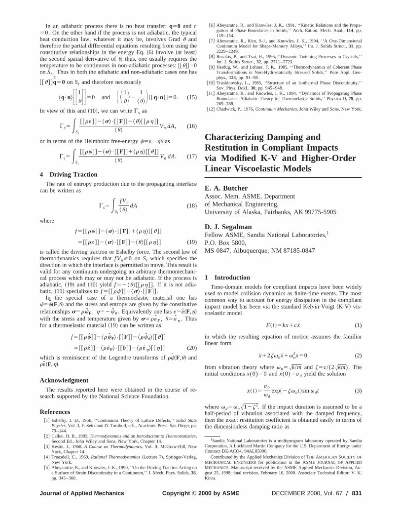
period K-V and Maxwell results are identical. The numericalsults for the standard linear model are shown for several valueh. The corresponding perturbation results~not shown! are essen-tially the same for smallh and z. It is seen that the restitutioncoefficient of the half-period K-V and Maxwell models indeevanishes asz→1. Hence, a finite damping constantcp may beassociated with purely plastic impacts in these two models whcp52Akm for K-V and cp5Akm/2 for Maxwell. In the modifiedK-V model, however, the restitution vanishes only asz→` so thatthe impact can never be purely plastic. It is also seen thatmodified K-V model has a restitution coefficient which is veclose to that of the half-period K-V and Maxwell models for smdamping ratios since the release times in these models fordamping are nearly the same. The advantages of analyticallytaining both the impact damping parameter~in terms of an experi-mentally obtained restitution coefficient! and the equivalent lineadamping constant for use in vibroimpact, together with the emore significant fact that all of the force boundary conditionssatisfied, leads to the conclusion that the Maxwell model isattractive choice for practical implementation in the modelingdissipative compliant impacts. However, the standard linmodel may also be helpful in ‘‘smoothing out’’ the K-V impacdiscontinuity. Especially if the impact duration is relatively lonor there are additional static forces on the impact surface,finite static deformation of this model is preferable to the flulike behavior of the Maxwell model. Furthermore, if the dampiis small and the instantaneous stiffness is large, then the imdynamics and restitution may be found as a perturbation of thfor the modified K-V model as was done here. Finally, furthwork is needed to extend these results to general planar and tdimensional collision theories and to include the use of kineand energetic restitution coefficients.

References@1# Yigit, A. S., Ulsoy, A. G., and Scott, R. A., 1990, ‘‘Dynamics of a Radial

Rotating Beam With Impact, Part 1: Theoretical and Computational ModeASME J. Vibr. Acoust.,112, pp. 65–70.

@2# Brach, R. M., 1991,Mechanical Impact Dynamics: Rigid Body Collision,John Wiley and Sons, New York.

@3# Brogliato, B., 1996,Nonsmooth Impact Mechanics: Models, Dynamics, aControl, Springer-Verlag, New York.

@4# Hunt, K. H., and Crossley, F. R. E., 1975, ‘‘Coefficient of RestitutioInterpreted as Damping in Vibroimpact,’’ ASME J. Appl. Mech.,42, pp.440–445.

@5# Herbert, R. G., and McWhannell, D. C., 1977, ‘‘Shape and FrequeComposition of Pulses From an Impact Pair,’’ J. Eng. Ind.,99, pp.513–518.

Fig. 2 Restitution coefficients for the half-period K-V and Max-well models „dotted …, modified K-V „solid …, and standard linearimpact model „numerical results … where hÄ0.0 „solid …, 0.05„long-dashed …, 0.2 „short-dashed …, and 0.4 „short-long-dashed …


e-s of

d

ere

theylllowob-

enreanofar

tgthed-gact

oseerree-tic

l,’’

d

n

cy

@6# Lee, T. W., and Wang, A. C., 1983, ‘‘On the Dynamics of Intermittent-MotioMechanisms,’’ ASME J. Mech. Des.,105, pp. 534–540.

@7# Khulief, Y. A., and Shabana, A. A., 1987, ‘‘A Continuous Force Model for thImpact Analysis of Flexible Multibody Systems,’’ Mech. Mach. Theory,22,No. 3, pp. 213–224.

@8# Luo, H., and Hanagud, S., 1998, ‘‘On the Dynamics of Vibration AbsorbWith Motion-Limiting Stops,’’ ASME J. Appl. Mech.,65, pp. 223–233.

@9# Mills, J. K., and Nguyen, C. V., 1992, ‘‘Robotic Manipulator CollisionsModeling and Simulation,’’ ASME J. Dyn. Syst., Meas., Control,114, pp.650–659.

@10# Haddad, Y. M., 1995,Viscoelasticity of Engineering Materials, Chapman andHall, New York.

@11# Nayfeh, A. H., 1981,Introduction to Perturbation Techniques, John Wiley andSons, New York.

Finite-Amplitude Elastic Instability ofPlane-Poiseuille Flow ofViscoelastic Fluids

R. E. Khayate-mail: [email protected]

N. Ashrafi

Department of Mechanical and Materials Engineering,University of Western Ontario, London,Ontario N6A 5B9, Canada

The purely elastic stability and bifurcation of the one-dimensioplane Poiseuille flow is determined for a large class of Oldrofluids with added viscosity, which typically represent polymerlutions composed of a Newtonian solvent and a polymeric solThe problem is reduced to a nonlinear dynamical system usingGalerkin projection method. It is shown that elastic normal streeffects can be solely responsible for the destabilization of the b(Poiseuille) flow. It is found that the stability and bifurcation picture is dramatically influenced by the solvent-to-solute viscoratio, «. As the flow deviates from the Newtonian limit and«decreases below a critical value, the base flow loses its stabiTwo static bifurcations emerge at two critical Weissenberg nubers, forming a closed diagram that widens as the level of eticity increases.@S0021-8936~00!00703-0#

1 IntroductionWhile the problem of stability of plane-Poiseuille flow~PPF!

has been extensively investigated for Newtonian fluids, relativlittle attention has been devoted to the flow of viscoelastic fluiThe presence of viscoelasticity is expected to dramatically athe stability and bifurcation picture in PPF, and yet no study hso far predicted the nonlinear bifurcation from the base flow. Tpresence of additional nonlinearities that are usually part ofrealistic constitutive model~@1#! are expected to lead to the depature from the Newtonian picture. Similarly to the case of TayloCouette flow, there is experimental evidence that the base floa channel may lose its stability as a result of fluid elasticity insthe tube~@2#!. This mechanism is now known as constitutive istability, as opposed to stick-slip induced instability. This mecnism of loss of stability should not be confounded with the showave instability due to a change in type of the field equatio

Contributed by the Applied Mechanics Division of THE AMERICAN SOCIETY OFMECHANICAL ENGINEERS for publication in the ASME JOURNAL OF APPLIEDMECHANICS. Manuscript received by the ASME Applied Mechanics Division, Ap28, 1999; final revision, July 27, 1999. Associate Technical Editor: A. K. Mal.


f

a

e

l

nee.e

s

il

i

sh

o

c

oy

at

e

-

oe

We,

r aon-

-

as

or.v-d

is

ndear

ureeioravior

which is known as Hadamard instability~@3#!. The emergence osurface instability at the exit of an extrusion die~sharkskin andmelt fracture! keeps hinting at the possibility of a link withhydrodynamic instability inside the channel, away and upstrefrom the exit~@4,5#!. However, linear stability analyses of chann~Couette and Poiseuille! flows, using elementary constitutivmodels, such as Maxwell and Oldroyd-B fluids, failed to assthat the base flow may be linearly unstable when the leveelasticity ~Weissenberg number! exceeds a critical level~@4,5#!.More recent studies based on more generalized constitutive mels of the Oldroyd class showed that the base flow in a chacan become unstable to small perturbations for some rangWeissenberg numbers~@6–8#!. These generalized constitutivmodels display a nonmonotonic shear-stress/shear-rate curverange of instability coincides with the negative slope of the strcurve. However, only linear stability analyses were carried ou

The present study focuses on the nonlinear constitutive inbility of the PPF of high-molecular-weight fluids. These fluids atypically composed of a Newtonian solvent and a polymeric sute. The Johnson-Segalman~JS! constitutive model is used, whichis a highly nonlinear equation, and is one of the very few contutive models that exhibit a nonmonotonic stress/shear-rate cuIt is thus expected that, while the presence of inertia and shthinning alone can destabilize the flow, fluid elasticity or normstresses will give rise to additional nonlinearities and couplamong the flow variables, making an already complex prob~due mainly to inertia! even more difficult to solve. Similarly toany flow in the transition regime, the PPF of viscoelastic fluinvolves a continuous range of excited spatio-temporal scalesorder to assess the influence of the arbitrarily many smaller lenand time scales on the flow, one would have to resort toresolution of the flow at the small-scale level. This issue remaunresolved since, despite the great advances in storage andof modern computers, it will not be possible to resolve all of tcontinuous ranges of scales in the transition regime.

It is by now well established that dynamical systems can bviable alternative to conventional numerical methods asprobes the nonlinear range of flow behavior~@9#!. Dynamical sys-tems are obtained using the Galerkin approximation. The veloand stress components assume truncated Fourier or other orthnal representations in space, depending on the boundary cotions. The expansion coefficients are functions of time alone, tleading to a nonlinear system upon projection of the equationto the various modes. The relative simplicity of dynamical stems, and the rich sequence of nonlinear flow phenomena exited by their solution, have been the major contributing factorstheir widespread use as models for examining the onset of nlinear behavior. The dynamical system approach has typicbeen used to handle simple flow configurations, and most parlarly Newtonian flows. Recently, this approach has beentempted for non-Newtonian flows in thermal convection~@10–12#! and rotating flow ~@13–17#!. For Taylor-Couette flow,comparison was carried out with the experiments of Muller et@18#, leading to excellent agreement~@15#!. A modal expansionsimilar to that in@14,15# is used to solve the current problem.

2 Problem Formulation and Solution ProcedureConsider the plane channel~Poiseuille! flow of an incompress-

ible viscoelastic fluid of densityr, relaxation timel, and viscosityh. In this study, only fluids that can be reasonably representeda single relaxation time and constant viscosity are considered.fluid considered here, is a polymer solution composed of a Ntonian solvent and a polymer solute of viscositieshs and hp ,respectively. Thereforeh5hs1hp . The velocity, time, space coordinates, pressure, and stress are nondimensionalized byd/l, l,d, hpU/d andhp /l, respectively. HereU is the maximum veloc-ity of the base Poiseuille flow, andd is the gap between the twplates. There are three important similarity groups in the probl


amel

ertof

od-nel

of

Thess

t.sta-reol-

ti-rve.earalngem

ds. Ingththeinspeede

e ane

ityogo-ndi-

husnss-hib-toon-lly

icu-at-

al.

byThew-

m,

namely, the Reynolds number, Re, the Weissenberg number,and the solvent-to-solute viscosity ratio,«, which are given, re-spectively, by

Re5d2r

hpl, We5

Ul

d, «5

hs

hp. (1)

The continuity and conservation of momentum equations fogeneral incompressible viscoelastic fluid are given in dimensiless form as

¹•u50, Redu

dt52We¹p1¹•t1«¹2u (2)

whereu is the velocity vector,p is the pressure,t is the polymericcontribution of the stress tensor,t is the time,d/dt is the substan-tial derivative operator, and¹ is the gradient operator. The constitutive equation adopted in this study belongs to theOldroydclass of incompressible viscoelastic fluids:

dt

dt2S 12

z

2D @~¹u! t•t1t•¹u#1

z

2@¹u•t1t•~¹u! t#

5¹u1~¹u! t (3)

where (¹u) t denotes the transpose of¹u. Equation~3! includesboth lower and upper-convective terms. It is often referred tothe Johnson-Segalman model~@19#!. Here zP@0,2#, which is adimensionless material~slip! parameter. The value ofz is a mea-sure of the contribution of nonaffine motion to the shear tensFor z50, the motion is affine and the Oldroyd-B model is recoered, whereas forz52, the motion is completely nonaffine anthe model is reduced to the Oldroyd-Jaumann model~@4#!. Whenz50 and hs50, the upper-convected Maxwell modelrecovered.

If the x-axis is taken to lie halfway between the two plates, ay is the coordinate in the transverse direction, then the total shstress corresponding to the base~Poiseuille! flow is given by

Txyb 5«g1

g

11z~22z!g2 5Wey (4)

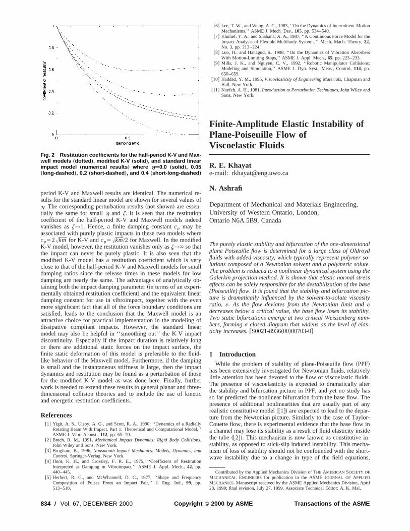
where g5du/dy is the shear rate andu is the velocity in thex-direction. Note that We is the dimensionless driving pressgradient. Equation~4! is perhaps the most revealing result of thJS model. It reflects the possibility of a nonmonotonic behavfor the stress/shear-rate relation. Indeed, Fig. 1 shows the behof the shear stress,Txy

b , as a function ofg for «P@0,1# and z

Fig. 1 Steady-state shear stress versus shear-rate curves forzÄ0.2 and ««†0,1‡. The loci of the two extrema are also shown,which join into one curve denoted here by gc . The curves inthe figure resemble the pressure Õstretch-ratio related to the in-flation of a Mooney-Rivlin material „see Fig. 2 in †20‡….


a

y

l

itun

n

as

d

f

i

s

that,

a

loss

s aatio

ere

a-

two

nge

2 foris-The

es

withsedf

luestlter-

-

es

hesach

rgee

hnge.ta-edthe

sta-nthe

iesace-e. 2

ter-isthealso

50.2. The curve«51 corresponds essentially to the Newtonilimit. For this value of the viscosity ratio, the elastic contributioto Txy

b in expression~4! is negligible. In this case Newton’s law oviscosity applies. The figure indicates that the stress curvesmonotonicity for«,1/8. Two extrema~a maximum and a mini-mum! appear, which tend to merge as« increases, as indicated bthe curve joining the loci of the extrema. The base flow is foundbe unstable for the range of the stress curves with negative sThis situation is reminiscent of the load/deformation behaviorelasticity. In the case of nonlinear inflation of a Mooney-Rivl~hyperelastic! membrane, for instance, the pressure also exhibisimilar behavior as function of the stretch ratio for varioMooney constants~@20#!. Upon comparison with the curves iFig. 1, the curve«50 is comparable to that of a Neo-Hookeasolid, while the curve for a Newtonian fluid («51) is comparableto the curve of a Hookean solid~see Fig. 2 in@20#!.

The solution of the system~1!–~2! is carried out using theGalerkin projection method. For one-dimensional disturbaalong the channel~x-axis!, the departure~from base flow! is re-duced to the axial velocity,u(y,t), normal stress differenceN(y,t), and shear stress,S(y,t). In this case, Eqs.~1!–~3! reduceto

Reut5«uyy1Sy (5a)

Nt52N12~WeS1Suy1Sbuy!. (5b)

St52S1uy1a~WeN1Nuy1Nbuy! (5c)

where a5z(z/221). Here Sb5g/11z(22z)g2 is the non-Newtonian contribution of the shear stress of the base flow,Nb52g2/11z(22z)g2 is the corresponding first normal stredifference. Note that a subscript in Eqs.~5! denotes partial differ-entiation. The flow departure is represented by series of Chdrasekhar functions, which satisfy the homogeneous~no-slip!boundary conditions~@15#!. A judicious selection process antruncation level is applied for the choice of the various modesorder to ensure the physical and mathematical coherence ofinal model.

3 Bifurcation and Stability PictureWhile the~linear! stability picture is somewhat predictable, th

bifurcation picture is far from being intuitively obvious. The bfurcation diagrams depend strongly on« andz. We thus monitorthe influence of the viscosity ratio by fixing the parameterz to 0.2

Fig. 2 Bifurcation diagrams for the normal stress difference,N„0,`…, at the center of the channel as function of We for zÄ0.2 and ««†0.06,0.08‡. The smallest diagram corresponds tothe highest viscosity ratio, «. As « exceeds a critical level „inthis case 1 Õ8…, the „closed … diagram reduces to zero, as thebase flow is always stable. The branches AB, CD, EF, and GH ofdiagram «Ä0.06 are unstable, whereas the branches BC, DE,EF, FG, and HA are stable.


nnflose

toope.inns as

n

ce

,

nds

an-

inthe

e-

and varying«. Figure 2 displays the resulting bifurcation diagramin the ~N, We! plane for«[email protected], 0.08#. The figure shows thedependence of the steady-state normal stress difference,N(0, ),at the center of the channel. Linear stability analysis assertsfor large« value ~.1/8!, the base flow is stable~to small pertur-bations! for any value of We. This situation corresponds tomonotonic shear-stress/shear-rate curve in Fig. 1. As« decreases,two extrema appear in the stress curves in Fig. 1, entraining aof stability of the base flow in between. For each«.1/8, a closedbifurcation diagram emerges as depicted in Fig. 2, which showwidening of the unstable range of We values as the viscosity rdecreases.

Although the case«50.06 will be discussed in detail below, wexamine first the evolution of the bifurcation and stability pictuas the flow deviates from close to the Newtonian limit~this limitis approached when the solvent-to-solute viscosity ratio,«, ishigh!. As « decreases below a critical value, two static bifurctions emerge at two critical values, Wec1 and Wec2 , of the Weis-senberg number as predicted by linear stability analysis. Thecritical points coincide with points A and E for the«50.06 dia-gram. The two bifurcating branches join over the unstable rato form a closed diagram. This is clearly illustrated for«50.08;the closed diagram intersects the We axis at Wec158.48 andWec2516.53. As« decreases further, the~closed! diagram wid-ens, and another closed diagram appears as depicted in Fig.«50.076. In this case, there are four critical values of the Wesenberg number that are present at 8.4, 17, 30, and 34.5.second range of We values~30 to 34.5! corresponds to unstablbase flow. A stable range exists between the two diagrams. A«decreases further, the two diagrams grow, come in contactone another, and finally merge to form a simply connected clodiagram as shown in Fig. 2 for«50.06. In this case, the range oinstability of the base flow becomes larger as it covers the va7.54,We,48.5~between A and E!. The figure also indicates thathe solution branch changes concavity, and presents regions anating in stability.

In general, and as typically depicted by the«50.06 diagram,there is an exchange of stability at the two critical points Wec1 ~A!and Wec2 ~E!, with the base flow losing its stability at Wec1 andregaining it at Wec2 . However, the base flow is not always unconditionally stable for We,Wec1 and We.Wec2 ; simulta-neously, the diagram«50.06 is not always unconditionally stablfor Wec1,We,Wec2 . We have indicated in Fig. 2 the varioubranches of alternating stability of the«50.06 diagram. Thus,branches AB, CD, EF, and GH are unstable, while the brancBC, DE, FG, and HA are stable. Consequently, close to ecritical point, just before Wec1 and just after Wec2 , there is abranch, BC and FG, respectively, to which the flow can conveif the perturbation is not small, similarly to what occurs in thvicinity of transcritical and subcritical bifurcations. Althougthere are stable and unstable nontrivial branches in the raWec1,We,Wec2 , there is total loss of stability of the base flowIn this range, only nonlinear velocity profiles are stable. The sbility of the branches at the two critical points was establishnumerically since linear stability analysis cannot be applied invicinity of the critical ~nonhyperbolic fixed! points.

It is, perhaps, at this stage that one begins to connect thebility and bifurcation picture to physical reality. It is well knowthat in real systems, physical instabilities are observed whenflow rate and/or the level of elasticity are high. These instabilitare believed to be potentially responsible for the onset of surfroughness in extrusion@10#. If we note that the flow rate is controlled by We, and the level of elasticity controlled by both Wand«, then we can clearly observe that the trend shown in Figconfirms that both the flow rate and fluid elasticity are the demining factors behind the destabilization of the base flow. Italso well known that instabilities are suspected to set in afterWeissenberg number has reached a certain value. This is


ue

d,tidb

cn

s

.e

v

uN

o

pc

-

i

t

w

tJ

d

a

m-e.ibu-ra-ks

andxt

oris-r-

ai-yce-

up-on

rim-ingob-ds.em

ed.the

are

ial

r..

inferred from Fig. 2, as the diagram corresponding to«50.06, forinstance, indicates that the base flow is practically unstable forwhole range We.7.5.

In summary, a nonlinear analysis is carried out to examineonset of constitutive instability and bifurcation for polymer soltions. Only elastic effects, which lead to the well-known Weissberg rod-climbing phenomenon, are responsible for the lossstability of the base~Poiseuille! flow. The viscoelastic model usedisplays nonmonotonicity of the shear-stress/shear-rate curvebelongs to the wider class ofOldroyd constitutive models thalead to the destabilization of channel flow. The bifurcation dgrams are obtained for the first time, and show how the seconflow evolves as one deviates from the Newtonian limit. Thefurcation diagrams are always closed and widen in range assolvent-to-solute viscosity decreases, thus reflecting the destazation observed in practice as the level of elasticity increases.emphasized that the present stability and bifurcation pictureresponds to perturbations of infinite wavelength, which maybe the most dangerous modes. Only a higher-dimensional stabanalysis can indicate whether the present findings are of phyrelevance.

AcknowledgmentsWe would like thank J. M. Floryan~UWO! for helpful com-

ments on the manuscript. This work is funded by the NatuSciences and Engineering Research Council of Canada.

References@1# Bird, R. B., Armstrong, R. C., and Hassager, O., 1987,Dynamics of Polymeric

Liquids, Vol. 1, 2nd Ed., John Wiley and Sons, New York.@2# Vinogradov, G. V., Malkin, A. Ya., Vanovskii, Yu G., Borisenkova, E. K

Yarlykov, B. V., and Berezheneya, G. V., 1972, J. Polym. Sci., Part A: GPap.,10, p. 1061.

@3# Joseph, D. D., Renardy, M., and Saut, J. C., 1985, ‘‘Hyperbolicity and Chaof Type in the Flow of Viscoelastic Fluids,’’ Arch. Ration. Mech. Anal.,87, p.213.

@4# Denn, M. M., 1990, ‘‘Issues in Viscoelastic Fluid Mechanics,’’ Annu. ReFluid Mech.,22, p. 13.

@5# Larson, R. G., 1992, ‘‘Instabilities in Viscoelastic Flows,’’ Rheol. Acta,31, p.213.

@6# Kolkka, R. W., Malkus, D. S., Hansen, M. G., and Ierley, G. R., 1988, ‘‘SpPhenomena of the Johnson-Segalman Fluid and Related Models,’’ J.Newtonian Fluid Mech.,29, p. 303.

@7# Malkus, D. S., Nohel, J. A., and Plohr, B. J., 1990, ‘‘Dynamics of Shear Flof a Non-Newtonian Fluid,’’ J. Comput. Phys.,87, p. 464.

@8# Georgiou, G. C., and Vlassopoulos, D., 1998, ‘‘On the Stability of the SimShear Flow of a Johnson-Segalman Fluid,’’ J. Non-Newtonian Fluid Me75, p. 77.

@9# Sell, G. R., Foias, C., and Temam, R., 1993,Turbulence in Fluid Flows: ADynamical Systems Approach, Springer-Verlag, New York.

@10# Khayat, R. E., 1994, ‘‘Chaos and Overstability in the Thermal ConvectionViscoelastic Fluids,’’ J. Non-Newtonian Fluid Mech.,53, p. 227.

@11# Khayat, R. E., 1995, ‘‘Nonlinear Overstability in the Thermal ConvectionViscoelastic Fluids,’’ J. Non-Newtonian Fluid Mech.,58, p. 331.

@12# Khayat, R. E., 1995, ‘‘Fluid Elasticity and Transition of Chaos in ThermConvection,’’ Phys. Rev. E,51, p. 380.

@13# Avgousti, M., and Beris, A. N., 1993, ‘‘Non-Axisymmetric Subcritical Bifurcations in Viscoelastic Taylor-Couette Flow,’’ Proc. R. Soc. London, Ser.A443, p. 17.

@14# Khayat, R. E., 1995, ‘‘Onset of Taylor Vortices and Chaos in ViscoelasFluids,’’ Phys. Fluids A,7, p. 2191.

@15# Khayat, R. E., 1997, ‘‘Low-Dimensional Approach to Nonlinear Overstabilof Purely Elastic Taylor-Vortex Flow,’’ Phys. Rev. Lett.,78, p. 4918.

@16# Graham, M. D., 1998, ‘‘Effect of Axial Flow on Viscoelastic Taylor-CouetInstability,’’ J. Fluid Mech.,360, p. 341.

@17# Ashrafi, N., and Khayat, R. E., 2000, ‘‘Finite Amplitude Taylor-Vortex Floof Weakly Shear-Thinning Fluids,’’ Phys. Rev. E,61, p. 1455.

@18# Muller, S. J., Shaqfeh, E. S. J., and Larson, R. G., 1993, ‘‘Experimental Sof the Onset of Oscillatory Instability in Viscoelastic Taylor-Couette Flow,’’Non-Newtonian Fluid Mech.,46, p. 315.

@19# Johnson, M. W., and Segalman, D., 1977, ‘‘A Model for Viscoelastic FluBehavior Which Allows Non-Affine Deformation,’’ J. Non-Newtonian FluiMech.,2, p. 278.

@20# Khayat, R. E., and Derdouri, A., 1994, ‘‘Inflation of Hyperelastic CylindricMembranes as Applied to Blow Moulding, Part I. Axisymmetric Case,’’ Int.Numer. Methods Eng.,37, p. 3773.


the

the-n-of

and

a-aryi-thebili-It isor-otilityical

ral

,n.

nge

.

rton-

w

leh.,

of

of

al

A,

tic

ty

e

udy.

id

lJ.

In-Plane Gravity Loadingof a Circular Membrane

R. O. TejedaResearch Assistant

E. G. LovellProfessor, Mem. ASME

R. L. EngelstadProfessor, Mem. ASME

Department of Mechanical Engineering, University ofWisconsin-Madison, Madison, WI 53706-1572

This paper develops the displacement field for a circular mebrane which is statically loaded by gravity acting in its planCoupled to the displacements are the stress and strain distrtions. The solution is applicable to the modeling of next genetion lithographic masks, ion-beam projection lithography masin particular. @S0021-8936~00!00803-5#

1 IntroductionIn most engineering applications, the displacement, stress,

strain fields induced by gravity are negligible. However, in negeneration~nonoptical! lithography masks used for semiconductdevice fabrication, it is critical to predict and compensate for dtortions which could potentially alter the quality of the microcicuit that is to be manufactured. Typically, the allowable error inlithographic mask is only a fraction of the microcircuit’s minmum feature size~@1#!. Since ion-beam projection lithograph~IPL! is targeting the production of sub-100 nm devices, displaments due to gravity can be significant.

An IPL mask is composed of a circular membrane that is sported by a relatively stiff frame and held in a vertical orientatiduring exposure~@2#!. It is typically made of silicon with a diam-eter on the order of 200 mm and 3.0-mm thickness. If the mask ismodeled as a circular membrane that is constrained on its peeter by a rigid ring and subjected to in-plane gravitational load~as shown in Fig. 1!, it can be considered as a plane stress prlem and solved directly by traditional applied elasticity methoTo the best of the authors’ knowledge, a solution to this problhas not been presented in the elasticity literature.

2 Solution DevelopmentThe position of an arbitrary point on the membrane is defin

by the polar coordinates (r ,u) with the origin taken at the centerAll translational displacement components are constrained atoutside radius,R. In general, radial~u! and circumferential (v)displacements which arise from the loading of the membranerelated to the radial strain (« r), circumferential strain («u), andshear strain (g ru) by strain-displacement equations, and to radnormal stress (s r), circumferential normal stress (su), and shearstress (t ru) by Hooke’s law, i.e.,

« r5]u

]r5

1

E~s r2nsu! (1)

Contributed by the Applied Mechanics Division of THE AMERICAN SOCIETY OFMECHANICAL ENGINEERS for publication in the ASME JOURNAL OF APPLIEDMECHANICS. Manuscript received by the ASME Applied Mechanics Division, Ap28, 1999; final revision, May 5, 2000. Associate Technical Editor: R. C. Benson


n

gt

,

s isffi-

rolvehich

-

uni-sr-

n-m-

«u5u

r1

1

r

]v]u

51

E~su2ns r ! (2)

g ru51

r

]u

]u1

]v]r

2vr

52~11n!

Et ru . (3)

Here,E is Young’s modulus andn is Poisson’s ratio. Equilibriumof the shaded element shown in Fig. 1 requires that

s r2su

r1

]s r

]r1

1

r

]t ru

]u2rg sinu50 (4)

1

r

]su

]u1

]t ru

]r1

2

rt ru2rg cosu50 (5)

where r and g are the material mass density and gravitatioacceleration, respectively.

A solution form which uses Airy’s stress function,f, can beexpressed as

s r51

r

]f

]r1

1

r 2

]2f

]u2 1F~r ,u! (6)

su5]2f

]r 2 1G~r ,u! (7)

t ru52]

]r S 1

r

]f

]u D (8)

where F(r ,u) and G(r ,u) are arbitrary functions. SubstitutinEqs.~6!–~8! into the equilibrium Eqs.~4! and~5! and subsequenintegration yields

G~r ,u!5rgr sinu1G2~r ! (9)

F~r ,u!5rgr sinu1F2~r !

r1

1

r E G2~r !. (10)

To preclude singular stresses, and without loss of generalityF2(u)5G2(r )50. Therefore,

s r51

r

]f

]r1

1

r 2

]2f

]u2 1rgr sinu (11)

su5]2f

]r 2 1rgr sinu. (12)

General forms off satisfying compatibility were originallygiven by Michell@3# for problems described in polar coordinateFrom Timoshenko’s~@4#! summary of this,

Fig. 1 In-plane gravity loading of a circular membrane


al

let

s.

f5a0 log r 1b0r 21c0r 2 log r 1d0r 2u1a08u1a1

2ru sinu

1~b1r 31a18r211b18r log r !cosu2

c1

2ru cosu

1~d1r 31c18r211d18r log r !sinu

1(n52

`

~anr n1bnr n121an8r2n1bn8r

2n12!cosnu

1(n52

`

~cnr n1dnr n121cn8r2n1dn8r

2n12!sinnu. (13)

A stress function which gives nonperiodic or singular stressenot admissible. Therefore, all the terms except those with coecients ofb0 , b1 , d1 , an , bn , cn , anddn will be dropped. So, forn52,3,4, . . .

f}r n~sinnu,cosnu! (14)

~s r ,su!}r n22~sinnu,cosnu! (15)

t ru}r n22~cosnu,sinnu!. (16)

On a circular edge, Eqs.~14!–~16! describe normal and sheastresses which vary harmonically. They are not necessary to sthe basic problem. Indeed, they may lead to displacements wcannot be zero at the boundaryr 5R. Thus, a solution may beconstructed using relevantf’s established by Michell, plus additional terms associated with the gravitational body forces:

f5b0r 21b1r 3 cosu1d1r 3 sinu. (17)

By the definition established in Eq.~8!,

t ru52b1r sinu22d1 r cosu. (18)

Due to the symmetric nature of the problem,t ru(r ,p/2)50.Therefore,b150. Similarly, Eqs.~11! and ~12! show that

s r52b012d1r sinu1rgr sinu (19)

su52b016d1r sinu1rgr sinu. (20)

Because it is associated with a hydrostatic loading such asform membrane prestress,b0 will also be discarded. This leaveone unknown,d1 , which can be identified by noting that the cicumferential normal strain is zero on the boundary, i.e.,«u(R,u)50. By using Eqs.~19!, ~20!, and~2!, this yields

d152rg

2

~12n!

~32n!(21)

and the stresses can now be written in the form

s r52rg

~32n!r sinu (22)

su52rgn

~32n!r sinu (23)

t ru5rg~12n!

~32n!r cosu. (24)

Employing Eqs.~1!–~3!, boundary conditions, and symmetry coditions gives the following strains and displacements in the mebrane:

« r~r ,u!52rg

E

~12n2!

~32n!r sinu (25)

«u~r ,u!50 (26)


a

lib-re

ksarlyich

or

the

ol-

gn,ng

ticc.,

y,

gateament

eamua-e’sareo aen-sultseg-

gis of

ics: N.

g ru~r ,u!52rg

E

~12n2!

~32n!r cosu (27)

u5rg

E

~12n2!

~32n!~r 22R2!sinu (28)

v5rg

E

~12n2!

~32n!~r 22R2!cosu. (29)

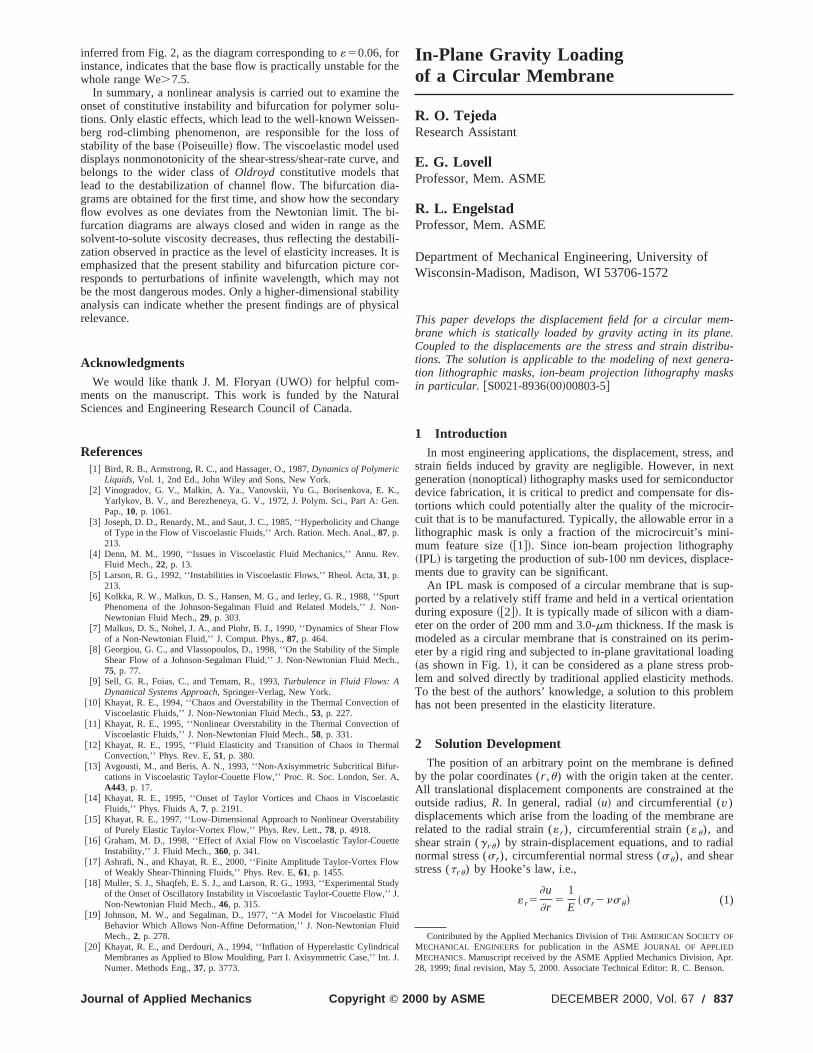
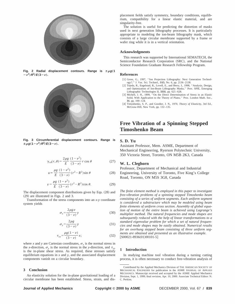
The displacement component distributions given by Eqs.~28! and~29! are illustrated in Figs. 2 and 3.

Transformation of the stress components into anx-y coordinatesystem yields

sx52rgn

~32n!y (30)

sy52rg

~32n!y (31)

txy5rg~12n!

~32n!x; (32)

wherex andy are Cartesian coordinates,sx is the normal stress inthe x-direction,sy is the normal stress in they-direction, andtxyis the in-plane shear stress. As required, these stresses sequilibrium equations inx andy, and the associated displacemecomponents vanish on a circular boundary.

3 ConclusionAn elasticity solution for the in-plane gravitational loading of

circular membrane has been established. Stress, strain, and

Fig. 2 Radial displacement contours. Range is Árg „1Àn2

…R2ÕE„3Àn….

Fig. 3 Circumferential displacement contours. Range isÁrg „1Àn2

…R2ÕE„3Àn….


tisfynt

adis-

placement fields satisfy symmetry, boundary conditions, equirium, compatibility for a linear elastic material, and asingularity-free.

The solution is useful for predicting the distortion of masused in next generation lithography processes. It is particulappropriate to modeling the ion-beam lithography mask, whconsists of a large circular membrane supported by a framewafer ring while it is in a vertical orientation.

AcknowledgmentsThis research was supported by International SEMATECH,

Semiconductor Research Corporation~SRC!, and the NationalScience Foundation Graduate Research Fellowship Program.

References@1# Gross, G., 1997, ‘‘Ion Projection Lithography: Next Generation Techn

ogy?,’’ J. Vac. Sci. Technol., B15, No. 6, pp. 2136–2138.@2# Tejeda, R., Engelstad, R., Lovell, E., and Berry, I., 1998, ‘‘Analysis, Desi

and Optimization of Ion-Beam Lithography Masks,’’ Proc. SPIE, EmergiLithographic Technologies II,3331, pp. 621–628.

@3# Michell, J. H., 1899, ‘‘On the Direct Determination of Stress in an ElasSolid, With Application to the Theory of Plates,’’ Proc. London Math. So31, pp. 100–124.

@4# Timoshenko, S. P., and Goodier, J. N., 1970,Theory of Elasticity, 3rd Ed.,McGraw-Hill, New York, pp. 132–135.

Free Vibration of a Spinning SteppedTimoshenko Beam

S. D. YuAssistant Professor, Mem. ASME, Department ofMechanical Engineering, Ryerson Polytechnic Universit350 Victoria Street, Toronto, ON M5B 2K3, Canada

W. L. CleghornProfessor, Department of Mechanical and IndustrialEngineering, University of Toronto, Five King’s CollegeRoad, Toronto, ON M5S 3G8, Canada

The finite element method is employed in this paper to investifree-vibration problems of a spinning stepped Timoshenko beconsisting of a series of uniform segments. Each uniform segmis considered a substructure which may be modeled using bfinite elements of uniform cross section. Assembly of global eqtion of motion of the entire beam is achieved using Lagrangmultiplier method. The natural frequencies and mode shapessubsequently reduced with the help of linear transformations tstandard eigenvalue problem for which a set of natural frequcies and mode shapes may be easily obtained. Numerical refor an overhung stepped beam consisting of three uniform sments are obtained and presented as an illustrative example.@S00021-8936~01!00101-5#

1 IntroductionIn studying machine tool vibration during a turning cuttin

process, it is often necessary to conduct free-vibration analys

Contributed by the Applied Mechanics Division of THE AMERICAN SOCIETY OFMECHANICAL ENGINEERS for publication in the ASME JOURNAL OF APPLIEDMECHANICS. Manuscript received and accepted by the ASME Applied MechanDivision, Sept. 1, 1999; final revision, Apr. 10, 2000. Associate Technical EditorC. Perkins.


lka

eocb

tes

g

;

nt,nt

-heum

ayin-is il-

ten

ty

heodbe

theding

ped

spinning stepped shaft. Bauer@1# presented an analytical study oa rotating uniform Euler-Bernoulli beam with various combintions of simple boundary conditions. Lee et al.@2# studied thefree vibration of a rotating Rayleigh shaft using the modal anasis approach and Galerkin’s method. Katz et al.@3# investigatedthe dynamic responses of a uniform rotating shaft subjectedmoving load in the axial direction using both Rayleigh and Tmoshenko beam theories. Zu and Han@4# presented analyticasolutions for free vibration of a spinning uniform Timoshenbeam with all combinations of the three classical boundconditions.

In this paper, free vibration of a rotating stepped Timoshenbeam is investigated using the finite element method. To enhathe accuracy of the computed eigenvalues and mode shapthree-node beam element, which permits the use of quintic pnomials as the interpolation function for both lateral displaments and bending angles, is utilized. For each of field variasix nodal quantities—the variable and its derivative with respto the axial coordinate at all three nodes are introduced toelement displacement vector. Two lateral deflections andbending angles at each axial location need be defined in bflexural vibration. Therefore, a three-node beam element hanodal variables.

Use of the finite element method makes it possible to reducefree-vibration problem of a spinning beam to a standard eigvalue problem for which all eigenvalues and eigenvectors maydetermined simultaneously. This is one advantage over the usan analytical method in which eigenvalues are determinedsearching for the roots of a characteristic equation. As an illustive example, natural frequencies of an overhung stepped aretained for several different spin rates.

2 Mathematical ProcedureIn this section, the equations of motion of a stepped beam

circular cross section, as shown in Fig. 1, are presented usininertial coordinate system. Parameters defining each segmenlength, diameter, and axial coordinate of the left-most plane.

2.1 Governing Differential Equations for a Substructure.In modeling the stepped beam, each segment is considered astructure. Within a substructure, the equations of motion maywritten as~@3#!

F FL2 0

0 L2G ]2

]t2 12VF 0 L1

2L1 0 G ]

]t1FL0 0

0 L0G G H ux

cx

uy

cy

J 5H 0000J

(1)

whereux anduy are lateral displacements of the beam centroidthe x andy directions, respectively;cx andcy are angles of rota-tion of the plane normal to the beam centroid, measured inxoz and yoz coordinate planes, respectively; the three operamatrices are defined as

L25FrA 0

0 rIG , L15F0 0

0 rIG ,

(2)

L05F 2kGA]2

]z2 kGA]

]z

2kGA]

]zkGA2EI

]2

]z2

G .

In Eq. ~2!, r is the volume mass density of the beam materialGis the shear modulus;E is the modulus of elasticity;A is thecross-sectional area;I is the second moment of area;k is the shearcorrection factor~0.9 for solid circular cross section,@4#!; V is thespin rate.


fa-

ly-

to ai-

ory

konces, aly-e-le,

ectthewoam24

theen-be

e ofby

tra-ob-

ofan

t are

sub-be

in

thetor

Assume that a uniform segmentk is modeled usingNe,k (k51,2, . . . ,Ns) three-node beam elements. Within each elemethe displacement vector$ue%k is related to the nodal displacemevector$qe%k by

$ue%k5@Ne~j!#$qe%k ~0<j< l e! (3)

wherej is the local coordinate;Ne(j) is the shape function matrix. The equations of motion of a uniform segment in terms of tnodal coordinate vector may be easily derived using the minimpotential energy principle or the Galerkin principle.

2.2 Assembly of Equations of Motion for the SteppedBeam. The global equations of motion for the entire beam mbe formulated by enforcing continuity conditions across eachterface between two adjacent substructures. The procedurelustrated here for a single interface at nodej with z5zj . The fourdisplacement and four force continuity conditions may be writin terms of the nodal displacements as

¦

ux

ux

cx

kx

uy

uy

cy

ky

§

z5zj2

531 0 0 0 0 0 0 0

0 a 12a 0 0 0 0 0

0 0 1 0 0 0 0 0

0 0 0 b 0 0 0 0

0 0 0 1 0 0 0 0

0 0 0 0 0 a 12a 0

0 0 0 0 0 0 1 0

0 0 0 0 0 0 0 b

435

ux

ux

cx

kx

uy

uy

cy

ky

6z5z

j1

5Cj5ux

ux

cx

kx

uy

uy

cy

ky

6z5z

j1

(4)

wherea andb are the shear rigidity ratio and the bending rigidiratio, defined as

a5~kGA!1

~kGA!2, b5

~EI !1

~EI !2. (5)

The continuity conditions may be implemented into tglobal equations of motion using the Lagrange multiplier meth~@5#!. The final equations of motion of a stepped beam maywritten as

@M #$q%1@G#$q%1@K #$q%50 (6)

where the global mass, gyroscopic and stiffness matrices forentire stepped beam may be formulated from the corresponmatrices for substructures and constraint matricesCj . Forexample, the global mass matrix for a three-segment stepbeam is

Fig. 1 An overhung stepped shaft


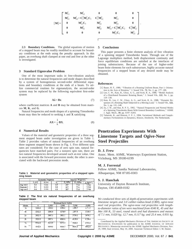
@M #5F M111 M12

1 0 0 0

M211 M22

1 1C1TM11

2 C1 C1TM12

2 M132 0

0 M212 C1 M22

2 M232 0

0 M312 M32

2 M332 1C2

TM113 C2 C2

TM123

0 0 0 M213 C2 M22

3

G .

o

s

d

-

usle

tionthendof

dertural

be

a-

is

e-

desE

withoseth-

seskg.

v..

2.3 Boundary Conditions. The global equations of motionof a stepped beam may be readily modified to account for bouary conditions at the ends using the penalty approach. Inpaper, an overhung shaft clamped at one end and free at theis investigated.

3 Standard Eigenvalue ProblemOne of the most important tasks in free-vibration analy

is to determine the natural frequencies and mode shapes descby a system of homogeneous second-order differential eqtions and boundary conditions at the ends of a beam. Tolize commercial routines for eigenanalysis, the second-orsystem may be replaced by the following equivalent first-orsystem

Ax5Bx (7)

where coefficient matricesA andB may be obtained from matricesM , K , andG.

Natural frequencies and mode shapes of a spinning Timoshebeam may then be reduced to seekingl andX satisfying

AX51

lBX. (8)

4 Numerical ResultsValues of the material and geometric properties of a three s

ment stepped beam under investigation are given in TableTable 2 provides values of natural frequencies of an overhthree segment stepped beam shown in Fig. 1. Five differentrates are considered. For the case of zero spin rate, naturaquencies have matched pairs. For a nonzero spin rate, thertwo natural frequencies developed around each at-rest value.is associated with the forward precession mode; the other is aciated with the backward precession mode.

Table 1 Material and geometric properties of a stepped spin-ning beam

Table 2 The first six natural frequencies of an overhungstepped beam


nd-thisther

isribedua-uti-derer

nko

eg-1.

ngpinfre-are

Onesso-

5 ConclusionsThis paper presents a finite element analysis of free vibra

of a spinning stepped Timoshenko beam. Through use ofLagrange multipliers method, both displacement continuity aforce equilibrium conditions are satisfied at the interfacesjoining substructures. Because of the use of higher-orbeam finite elements for each substructure, highly accurate nafrequencies of a stepped beam of any desired mode mayobtained.

References@1# Bauer, H. F., 1980, ‘‘Vibration of a Rotating Uniform Beam, Part 1: Orient

tion in the Axis of Rotation,’’ J. Sound Vib.,72, No. 2, pp. 177–189.@2# Lee, C. W., Katz, R., Ulsoy, A. G., and Scott, R. A., 1988, ‘‘Modal Analys

of a Distributed Parameter Rotating Beam,’’ J. Sound Vib.,122, No. 1, pp.119–130.

@3# Katz, R., Lee, C. W., Ulsoy, A. G., and Scott, R. A., 1988, ‘‘Dynamic Rsponses of a Rotating Shaft Subjected to a Moving Load,’’ J. Sound Vib.,122,No. 1, pp. 131–148.

@4# Zu, J. W., and Han, R. P. S., 1992, ‘‘Natural Frequencies and Normal Moof a Spinning Timoshenko Beam With General Boundary Conditions,’’ ASMJ. Appl. Mech.,59, pp. S197–S203.

@5# Tabarrok, B., and Rimrott, F. P. J., 1994,Variational Methods and Comple-mentary Formulations in Dynamics, Kluwer, Dordrecht, The Netherlands.

Penetration Experiments WithLimestone Targets and Ogive-NoseSteel Projectiles

D. J. FrewAssoc. Mem. ASME, Waterways Experiment Station,Vicksburg, MS 39180-6199

M. J. ForrestalFellow ASME, Sandia National Laboratories,Albuquerque, NM 87185-0303

S. J. HanchakUniversity of Dayton Research Institute,Dayton, OH 45469-0182

We conducted three sets of depth-of-penetration experimentslimestone targets and 3.0 caliber-radius-head (CRH), ogive-nsteel rod projectiles. The ogive-nose rod projectiles with lengto-diameter ratios of ten were machined from 4340 Rc 45 and AerMet 100 Rc 53 steel, round stock and had diameters and masof 7.1 mm, 0.020 kg; 12.7 mm, 0.117 kg; and 25.4 mm, 0.931

Contributed by the Applied Mechanics Division of THE AMERICAN SOCIETY OFMECHANICAL ENGINEERS for publication in the ASME JOURNAL OF APPLIEDMECHANICS. Manuscript received by the ASME Applied Mechanics Division, No29, 1999; final revision, May 10, 2000. Associate Technical Editor: I. M. Daniel


j1i

e

eeah

g

tc

e

m

ae

r

oeF

ash

e

tt

o

for

ribe

tionsec-rlyarens.

is

lleri-

eic-

.1,ten

her in-

e-

qua-

e-tio

peri-m,

ndherop-howted

Powder guns or a two-stage, light-gas gun launched the protiles at normal impacts to striking velocities between 0.4 andkm/s. In addition, we present an analytical penetration equatthat described the target resistance by its density and a strenparameter determined from depth of penetration versus strikvelocity data.@S0021-8936~01!00201-X#

IntroductionSeveral authors have written review articles that discuss

many analytical, computational, and experimental methods uto study the broad field of penetration mechanics~@1–5#!. Theresponses of the projectiles and targets depend strongly onproblem geometry, materials, and impact conditions. Becamany penetration mechanisms are possible, experimental obstions usually precede and guide analytical or computational mels. For this study, post-test observations showed a conical ecrater with a depth of two or more projectile diameters followby a circular penetration channel or tunnel with nearly the projtile diameter. For recent penetration studies with 6061-T6511minum targets~@6,7#! we could obtain post-test radiographs of tpenetration channels. However, we could obtain post-test obvations of the limestone penetration channels only after the tarwere split with the techniques used by stone masons. The protiles recovered from the targets had small mass losses causeabrasion, but the overall nose shapes before and after penetrlooked very similar. We previously observed similar post-test,get channels and abraded projectiles with our studies on contargets~@8,9#!. However, the concrete targets abraded the nosemore severely than the limestone targets.

Based on penetration data sets with three projectile scalespresent an analytical penetration equation that describes targsistance by a parameter determined from penetration depth vestriking velocity data. Our limestone penetration equation is silar to that previously derived for concrete targets~@10#!. However,for limestone targets, we observed a noticeable decrease intarget resistance parameter as the projectile diameters increSo for the limestone targets, the target resistance parametequal to a constant term plus a term that depends on the projediameter. We hypothesize that the penetration equation willreasonably accurate for larger scale projectiles, but data fmuch more expensive field tests must be obtained to confirmhypothesis.

The limestone targets were quarried and cut by the Elliot StCompany.1 In the rock mechanics literature, this particular limstone is often called Salem, Indiana, or Bedford limestone.this study, we conducted unconfined compression tests and striaxial compression tests on samples cored from representblocks and from individual targets before the penetration teMaterial properties from our targets are nearly the same as treported by Fossum, Senseny, Pfeifle, and Mellegard@11#.

As previously mentioned, our penetration equation containtarget strength constant that is determined from penetration dversus striking velocity data. While this methodology providesaccurate and convenient engineering equation, the detailedsponse mechanisms for the target are not modeled. The auare not aware of any rigorous target models for rock penetraproblems, but Lagrangian computational models that use adapmeshing techniques have shown promise for brittle ceramicgets~@12,13#!. Detailed computational approaches that model tget responses also require a broad array of quasi-static andnamic material properties data. For limestone, examples of smaterials experiments and data include~1! quasi-static, triaxialcompression experiments~@11#!, ~2! split Hopkinson bar experi-ments~@14–16#!, ~3! shock wave studies~@17#!, ~4! dynamic ten-sile failure with planar-impact techniques~@18,19#!, and ~5!

1Elliot Stone Company, 3326 Mitchell Road, Bedford, IN 47421.


ec-.9

ongthing

thesed

theuserva-

od-ntrydc-lu-eser-etsjec-d byationar-retetips

, wet re-rsusi-

thesed.r is

ctilebeomour

ne-or

ometivets.ose

s apth

anre-

horsiontivetar-ar-

dy-me

compression-shear loading with plate impact experiments~@20#!.Data from other experimental techniques may also be requireda careful target analysis.

In the next sections, we present the penetration model, descthe experiments, and present our results and conclusions.

Penetration ModelFor both limestone and concrete targets, post-test observa

showed a conical entry crater with a depth of two or more projtile diameters followed by a circular channel or tunnel with neathe projectile diameter. The limestone penetration equationssimilar to the previously published concrete penetration equatioFrom Forrestal, Altman, Cargile, and Hanchak@10#, depth of pen-etration P for an ogive-nose projectile and a concrete targetgiven by

P5m

2pa2rNlnS 11

NrV12

R D 14a, P.4a (1a)

N58c21

24c2 , V125

mVs224pa3R

m14pa3Nr(1b)

in which the ogive-nose rod projectile is described by massm,shank radiusa, and caliber-radius-headc. The target is describedby densityr and the target strength constantR. The strength con-stant is determined from

R5NrVs

2

S 114pa3Nr

m DexpF2pa2~P24a!Nr

m G21

(2)

whereVs is striking velocity. For a set of experiments, we hold aparameters constant and vary striking velocity. From each expment, we measure striking velocityVs and penetration depthP, soR can be determined from~2! for each experiment. We then takthe average value ofR from the data set and compare the predtion from ~1! with the measured values ofVs andP. For this studywith limestone targets, ogive-nose steel rod projectiles with 712.7, and 25.4-mm diameters and a length-to-diameter ratio ofhave values ofR5913, 787, and 693 MPa, respectively. Thus, ttarget resistance decreases as the projectile shank diametecreases. We found that for these limestone targets

R5K1k~2ao/2a! (3)

in which K and k are constants obtained from data fits, 2ao is areference projectile diameter, and 2a is the projectile diameter.We show later that withK5607 MPa, k586 MPa, and 2ao525.4 mm, we accurately recover the measured values ofR foreach of the three data sets.

In summary, the procedure used to calculateR from penetrationdepth data for a fixed projectile is the same for concrete or limstone targets. However, for limestone targets,R depends on theprojectile shank diameter. Thus, we can use the penetration etions ~1a! and ~1b! for limestone whenR is given by~3!.

ExperimentsWe conducted three sets of penetration experiments~a total of

30 experiments! with ogive-nose steel rod projectiles and limstone targets. All projectiles had a total length-to-diameter raof ten and 3.0 caliber-radius-head~CRH! nose shapes. Theshank diameters and masses for each of the three sets of exments were 7.1 mm, 0.020 kg; 12.7 mm, 0.117 kg; and 25.4 m0.931 kg.

Limestone Targets. The limestone targets were quarried acut by the Elliot Stone Company of Bedford, IN. We obtained ttargets in three batches from nearby sites. Nominal material perties for the three target batches are given in Table 1 and sminimal variations among the batches. In addition, we conduc


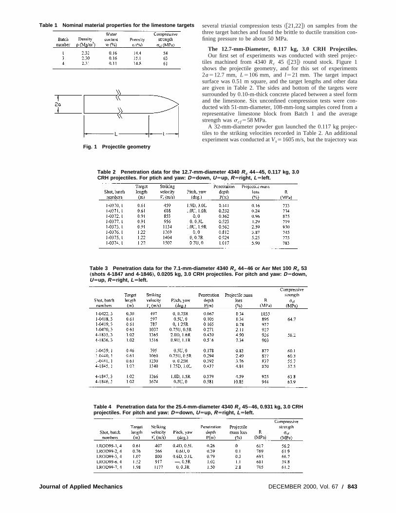
on-

ec-

ntstdataereormcon-m aage

ec-al

s
Fig. 1 Projectile geometry
Table 1 Nominal material properties for the limestone targets


several triaxial compression tests~@21,22#! on samples from thethree target batches and found the brittle to ductile transition cfining pressure to be about 50 MPa.

The 12.7-mm-Diameter, 0.117 kg, 3.0 CRH Projectiles.Our first set of experiments was conducted with steel proj

tiles machined from 4340Rc 45 ~@23#! round stock. Figure 1shows the projectile geometry, and for this set of experime2a512.7 mm, L5106 mm, andl 521 mm. The target impacsurface was 0.51 m square, and the target lengths and otherare given in Table 2. The sides and bottom of the targets wsurrounded by 0.10-m-thick concrete placed between a steel fand the limestone. Six unconfined compression tests wereducted with 51-mm-diameter, 108-mm-long samples cored frorepresentative limestone block from Batch 1 and the averstrength wassc f558 MPa.

A 32-mm-diameter powder gun launched the 0.117 kg projtiles to the striking velocities recorded in Table 2. An additionexperiment was conducted atVs51605 m/s, but the trajectory wa

Table 2 Penetration data for the 12.7-mm-diameter 4340 Rc 44–45, 0.117 kg, 3.0CRH projectiles. For ptich and yaw: DÄdown, UÄup, RÄright, LÄleft.

Table 3 Penetration data for the 7.1-mm-diameter 4340 Rc 44–46 or Aer Met 100 Rc 53„shots 4-1847 and 4-1846 …, 0.0205 kg, 3.0 CRH projectiles. For pitch and yaw: DÄdown,UÄup, RÄright, LÄleft.

Table 4 Penetration data for the 25.4-mm-diameter 4340 Rc 45–46, 0.931 kg, 3.0 CRHprojectiles. For pitch and yaw: DÄdown, UÄup, RÄright, LÄleft.


ua

inet of

tiles

this

ik-e-hedsure-pro-

nedThetwoeterex-

togli-Thets is

inAerfex-

nedren100

ma-

curved and the projectile exited the side of the target at a deptabout 0.65 m. The projectiles were fitted with sabots and obttors that separated from the projectiles before impact. Four ldiode systems measured striking velocities and orthogonal ragraphs measured pitch and yaw angles. The target resistanR

Fig. 2 Post-test photographs of the 25.4-mm-diameterprojectiles


h ofra-ser

dio-ce

was calculated from~2! for each experiment and recordedTable 2. The average target resistance parameter for this sexperiments isR5787 MPa.

The 7.1-mm-Diameter 0.020 kg, 3.0 CRH Projectiles. Oursecond set of experiments was conducted with steel projecmachined from both 4340Rc 45 and Aer Met 100Rc 53 ~@24#!round stock. Figure 1 shows the projectile geometry, and forset of experiments 2a57.11 mm,L559.3 mm, andl 511.8 mm.A 20-mm-powder gun launched the 0.020 kg projectiles to string velocities of 1230 m/s. For the larger striking velocities rcorded in Table 3, a two-stage 50/20 mm light-gas gun launcthe projectiles. The same target geometries and ballistics meaments as those described for the 12.7-mm-diameter 0.117 kgjectiles were used for this set of experiments.

For this second set of experiments, we performed unconficompression tests on two samples cored from the targets.compressive strengths listed in Table 3 are the average ofunconfined compression tests conducted with 50-mm-diam108-mm-long cores. In addition, we conducted penetrationperiments from both Batch 1 and Batch 3 limestone targetscompare results from the two batches. We show later negible differences in the penetration data from both batches.average target resistance parameter of this set of experimenR5913 MPa.

We also conducted an experiment with a 4340Rc 45 projectileat Vs51649 m/s. That projectile severely bent and turned withthe target. Table 3 shows two experiments conducted withMet 100Rc 53 projectiles. Shot 4-1846 with a striking velocity o1674 m/s had a nearly straight trajectory. We then conductedperiments atVs51749, 1826, and 1863 m/s with Aer Met 100Rc53 projectiles and these projectiles severely bent and turwithin the targets. Piekutowski, Forrestal, Poormon, and War@7# discusses in detail the better performance of the Aer MetRc 53 projectiles.

The 25.4-mm-diameter 0.931 kg, 3.0 CRH Projectiles. Ourthird set of experiments was conducted with steel projectiles

Fig. 3 Data and model predictions for the limestone targets


c

-

r

ir

e

notr

t

t

s

geo

t

0

n,uire

k

a

o

t ofD/.S.Pro-

of

of

k,

f

tes

ndith.99,ec-g.,

tra-. J.

en-act

‘Anon-

95,f a

of

ary-

theo-

d

, pp.

of

of

in

in

,

n,

us-

chined from 4340Rc 45 round stock. Figure 1 shows the projetile geometry, and for this set of experiments 2a525.4 mm, L5212 mm, andl 542 mm. The target impact surface was 1.02square and the target lengths are given in Table 4. The sidesbottom of the targets were surrounded by 0.10-m-thick concplaced between a steel form and the limestone. An 83-mm powgun launched the 0.931 kg projectiles to the striking velocitrecorded in Table 4. The same experimental methods used foother data sets were also used to obtain the results given in T4. Data in Table 4 were limited toVs51177 m/s because of thsize and mass of the targets. The average value ofR for this set ofexperiments wasR5693 MPa.

Results and DiscussionAs previously discussed, post-test target observations for

experiments summarized in Tables 2, 3, and 4 showed a coentry crater with a depth of two or more projectile diameters flowed by a circular penetration tunnel with nearly the projecdiameter. However, we made post-test observations only aftetargets were split with the techniques used by stone masons.ure 2 shows post-test photographs of the 25.4-mm-diameterjectiles, and mass losses are given in Table 4. These recovprojectiles lost mass caused by abrasion, but the nose shapefore and after penetration have similar shapes. Post-test projecfrom the other data sets~Tables 2 and 3! had shapes similar tothose shown in Fig. 2.

Figure 3 shows depth of penetrationP versus striking velocityVs for the data in Tables 2, 3, and 4. For the model, we useaverage value ofR calculated from~2! for the experiments ineach data set. For the 7.1, 12.7, and 25.4-mm-diameter projecthe average target resistance parameter isR5913, 787, and 693MPa, respectively. For projectile diameters not tested instudy, we recommend~3! be used to calculateR. Equation~3!with K5607 MPa,k586 MPa, and 2ao525.4 mm accurately re-cover the measured values ofR from each of the three data setWe hypothesize that the penetration equations~~1! and ~3!!for this limestone target will be reasonably accurate for larscale projectiles, but data from much more expensive field twith larger diameter projectiles must be obtained to confirmhypothesis.

SummaryWe conducted sets of penetration experiments into limest

targets with three scales of geometrically similar projectiles. Togive-nose rod projectiles with a length-to-diameter ratio ofwere machined from 4340Rc 45 and Aer Met 100Rc 53 steel,round stock and had diameters and masses of 7.1 mm, 0.0212.7 mm, 0.117 kg; and 25.4 mm, 0.931 kg. For the 4340Rc 45and Aer Met 100Rc 53 steel projectiles, penetration depth icreased as striking velocity increased to 1500 and 1700 m/sspectively. For larger striking velocities, the projectiles bent ding penetration without nose erosion, deviated from the shot land exited the sides of the target or turned severely in the ta

Based on data sets with these three projectile scales, we pran analytical penetration equation based on a target strengthrameter that is determined from penetration depth versus strivelocity data. We show that the target resistance parameterpends on the projectile shank diameter and present an equthat describes this diameter dependence. We hypothesize thapenetration equations for this limestone target will give accurpredictions for larger scale projectile, but data from much mexpensive field tests with larger diameter projectiles must betained to confirm our hypothesis.


-

mandetederesthe

able

theicall-

iletheFig-pro-ereds be-tiles

the

iles,

his

.

erstsur

oneheen

kg;

-re-r-

ne,get.sentpa-

ingde-tiont theatere

ob-

AcknowledgmentsThis work was supported by the United States Departmen

Energy under Contract DE-AC04-94AL85000, the Joint DoDOE Munitions Technology Development Program, and the UArmy Corps of Engineers Hardened Structures Researchgrams~AT22 and AT40!.

References@1# Backman, M. E., and Goldsmith, W., 1978, ‘‘The Mechanics of Penetration

Projectiles Into Targets,’’ Int. J. Eng. Sci.,16, pp. 1–99.@2# Anderson, C. E., and Bodner, S. R., 1988, ‘‘Ballistic Impact: The Status

Analytical and Numerical Modeling,’’ Int. J. Impact Eng.,7, pp. 9–35.@3# Hohler, V., and Stilp, A. J., 1990, ‘‘Long-Rod Penetration Mechanics,’’High

Velocity Impact Dynamics, J. A. Zukas, ed., John Wiley and Sons, New YorChapter 5.

@4# Recht, R., 1990, ‘‘High Velocity Impact Dynamics: Analytical Modeling oPlate Penetration Dynamics,’’High Velocity Impact Dynamics, J. A. Zukas,ed., John Wiley and Sons, New York, Chapter 7.

@5# Corbett, G. G., Reid, S. R., and Johnson, W., 1996, ‘‘Impact Loading of Plaand Shells by Free-Flying Projectiles: A Review,’’ Int. J. Impact Eng.,18, pp.141–230.

@6# Warren, T. L., and Forrestal, M. J., 1998, ‘‘Effects of Strain Hardening aStrain-Rate Sensitivity on the Penetration of Aluminum Targets WSpherical-Nosed Rods,’’ Int. J. Solids Struct.,35, Nos. 28–29, pp. 3737–3753

@7# Piekutowski, A. J., Forrestal, M. J., Poormon, K. L., and Warren, T. L., 19‘‘Penetration of 6061-T6511 Aluminum Targets by Ogive-Nose Steel Projtiles With Striking Velocities Between 0.5 and 3.0 km/s,’’ Int. J. Impact En23, pp. 723–734.

@8# Forrestal, M. J., Frew, D. J., Hanchak, S. J., and Brar, N. S., 1996, ‘‘Penetion of Grout and Concrete Targets With Ogive-Nose Steel Projectiles,’’ IntImpact Eng.,18, No. 5, pp. 465–476.

@9# Frew, D. J., Hanchak, S. J., Green, M. L., and Forrestal, M. J., 1998, ‘‘Petration of Concrete Targets With Ogive-Nose Steel Rods,’’ Int. J. ImpEng.,21, No. 6, pp. 489–497.

@10# Forrestal, M. J., Altman, B. S., Cargile, J. D., and Hanchak, S. J., 1994, ‘Empirical Equation for Penetration Depth of Ogive-Nose Projectiles Into Ccrete Targets,’’ Int. J. Impact Eng.,15, No. 4, pp. 395–405.

@11# Fossum, A. F., Senseny, P. E., Pfeifle, T. W., and Mellegard, K. D., 19‘‘Experimental Determination of Probability Distributions for Parameters oSalem Limestone Cap Plasticity Model,’’ Mech. Mater.,21, pp. 119–137.

@12# Ortiz, M., 1996, ‘‘Computational Micromechanics,’’ Comput. Mech.,18, pp.321–338.

@13# Camacho, G. T., and Ortiz, M., 1997, ‘‘Adaptive Lagrangian ModellingBallistic Penetration of Metallic Targets,’’ Comput. Meth., Appl. Eng.,142,pp. 269–301.

@14# Green, S. J., and Perkins, R. D., 1972, ‘‘Uniaxial Compression Tests at Ving Strain Rates on Three Geologic Materials,’’Proc. 10th Symp. Rock Me-chanics, Inst. Mining Metallurgical and Petroleum Engrs., K. E. Gray, ed.,AIME, New York, pp. 35–54.

@15# Lindholm, U. S., Yeakley, L. M., and Nagy, A., 1974, ‘‘The Dynamic Strengand Fracture Properties of Dresser Basalt,’’ Int. J. Rock Mech. Min. Sci. Gmech. Abstr.,II , pp. 181–191.

@16# Lipkin, J., Grady, D. E., and Campbell, J. D., 1977, ‘‘Dynamic Flow anFracture of Rock in Pure Shear,’’Proc. 18th U.S. Symp. Rock Mechanics, F.Wang and G. B. Clark, eds., Colorado School of Mines Press, Golden, Co3 B2–1, 3 B2–7.

@17# Larson, D. B., and Anderson, G. D., 1979, ‘‘Plane Shock Wave StudiesPorous Geological Media,’’ J. Geophys. Res.,84, No. B9, pp. 4592–4600.

@18# Grady, D. E., and Hollenbach, R. E., 1979, ‘‘Dynamic Fracture StrengthRock,’’ Geophys. Res. Lett.,6, No. 2, pp. 73–76.

@19# Ahrens, T. J., and Rubin, A. M., 1993, ‘‘Impact-Induced Tensional FailureRock,’’ J. Geophys. Res.,98, No. E1, pp. 1185–1203.

@20# Aidun, J. B., and Gupta, Y. M., 1995, ‘‘Shear and Compression WavesShocked Calcium Carbonate,’’ J. Geophys. Res.,100, No. B2, pp. 1955–1980.

@21# Farmer, I., 1983,Engineering Behavior of Rocks, 2nd Ed., Chapman and HallNew York.

@22# Jaeger, J. C., and Cook, N. G. W., 1979,Fundamentals of Rock Mechanics,3rd Ed., Chapman and Hall, New York.

@23# Brown, W. F., Mindlin, H., and Ho, C. Y., 1996,Aerospace Structural MetalsHandbook, Vol. 1, Code 1206, CINDAS/USAF CRDA Handbooks OperatioPurdue University, West Lafayette, IN.

@24# Dahl, J., 1991, ‘‘Aer Met 100—An Advanced Steel for the Aerospace Indtry,’’ Adv. Mat. Tech. Int., pp. 40–45.


tiz

tr

nh

e

te

u

elds,,ou-

ad-

a-

Eccentric Crack in a PiezoelectricStrip Under ElectromechanicalLoading

Jeong Woo ShinResearcher, Korea Aerospace Research Institute,52 Oun-dong, Yusong-gu, Taejon 306-333, Korea

Soon Man KwonGraduate Student

Kang Yong Lee1

Professor

Department of Mechanical Engineering, Graduate SchoYonsei University, Seoul 120-749, Korea

1 IntroductionWith an increasingly wide application media in engineering,

study on the crack problem in piezoelectric media has recemuch interest. In this paper, we apply the theory of linear pieelectricity to the electroelastic problem of a finite eccentric craoff the center line in a piezoelectric ceramic strip under antiplashear loading. The continuous crack boundary conditionadopted. By using integral transform techniques, the problemreduced to the solution of a Fredholm integral equation ofsecond kind, which is obtained from two pairs of dual integequations. Numerical results for the energy release rate are shgraphically.

2 Problem Statement and Method of SolutionConsider a piezoelectric medium in the form of an infinite

long strip containing a finite eccentric crack off the center liparallel to the edges subjected to the combined antiplane meccal and in-plane electric loads. A set of Cartesian coordina(x,y,z) is attached to the center of the crack. The total thicknof the strip is 2h(5h11h2), whereh1(5h2e) is the distancebetween the top surface of the strip and the crack planeh2(5h1e) is that between the bottom surface of the strip athe crack plane.e denotes the distance from the center line of tstrip to the crack plane. The crack is situated along the virtinterface (2a<x<a, y50). Because of the assumed symmein geometry and loading, it is sufficient to consider the problfor 0<x,` only. Antiplane governing equations are simplifieto

c44¹2w~ i !1e15¹

2f~ i !50, (1)

e15¹2w~ i !2d11¹

2f~ i !50, (2)

where ¹25]2/]x21]2/]y2 is the two-dimensional Laplace operator, w( i ), f ( i ) ( i 51,2), c44, d11, and e15 are the out-of-plane displacement, the electric potential, the elastic modmeasured in a constant electric field, the dielectric permittivmeasured at a constant strain, and the piezoelectric consrespectively. Superscripti ( i 51,2) stands for upper and loweregions, respectively. The boundary conditions are writtenfollows:

1To whom correspondence should be addressed.Contributed by the Applied Mechanics Division of THE AMERICAN SOCIETY OF

MECHANICAL ENGINEERS for publication in the ASME JOURNAL OF APPLIEDMECHANICS. Manuscript received by the ASME Applied Mechanics Division, Ja19, 2000; final revision, Apr. 20, 2000. Associate Technical Editor: D. Kouris.


ol,

hevedo-ckneisis

healown

lyeani-tesss

andndheualrymd

-

lusitytant,ras

syz~ i !~x,0!50, ~0<x,a!, (3)

w~1!~x,01!5w~2!~x,02!, ~a<x,`!, (4)

Dy~1!~x,01!5Dy

~2!~x,02!, ~0<x,a!, (5)

Ex~1!~x,01!5Ex

~2!~x,02!, ~0<x,a!, (6)

f~1!~x,01!5f~2!~x,02!, ~a<x,`!, (7)

syz~1!~x,01!5syz

~2!~x,02! ~a<x,`!,(8)

Dy~1!~x,01!5Dy

~2!~x,02!, ~a<x,`!.

Case 1: syz~1!~x,h1!5syz

~2!~x,2h2!5t0 ,(9)

Dy~1!~x,h1!5Dy

~2!~x,2h2!5D0 ,

Case 2: gyz~1!~x,h1!5gyz

~2!~x,2h2!5g0 ,(10)

Ey~1!~x,h1!5Ey

~2!~x,2h2!5E0 ,

Case 3: syz~1!~x,h1!5syz

~2!~x,2h2!5t0 ,(11)

Ey~1!~x,h1!5Ey

~2!~x,2h2!5E0 ,

Case 4: gyz~1!~x,h1!5gyz

~2!~x,2h2!5g0 ,(12)

Dy~1!~x,h1!5Dy

~2!~x,2h2!5D0 ,

wheresyz( i ) , gyz

( i ) , Dy( i ) , andEj

( i ) ( j 5x,y) are the shear stress, thshear strain, the electric displacements, and the electric fierespectively, andt0 , D0 , g0 , andE0 are a uniform shear stressdisplacement, shear strain, and electric field, respectively. A Frier transform is applied to Eqs.~1! and ~2!, and the results are

w~ i !~x,y!52

p E0

`

$A1~ i !~s!cosh~sy!1A2

~ i !~s!sinh~sy!%

3cos~sx!ds1a0y, (13)

f~ i !~x,y!52

p E0

`

$B1~ i !~s!cosh~sy!1B2

~ i !~s!sinh~sy!%

3cos~sx!ds2b0y, (14)

whereAj( i ) , Bj

( i ) ( j 51,2) are the unknowns to be solved.a0 ,b0are real constants, which will be determined from the edge loing conditions. Applying Eqs.~8!–~12!, and considering Eqs.~3!–~7!, we obtain the following two simultaneous dual integral equtions:

E0

`

sF~s!FMA~s!1e15

c44MB~s!Gcos~sx!ds5

p

2

c0

c44,

~0<x,a!,(15)

E0

`

MA~s!cos~sx!ds50, ~a<x,`!,

E0

`

sMB~s!sin~sx!ds50, ~0<x,a!,

(16)

E0

`

MB~s!cos~sx!ds50, ~a<x,`!,

where

2MA~s!5A1~1!~s!2A1

~2!~s!, 2MB~s!5B1~1!~s!2B1

~2!~s!, (17)

F~s!5tanh~sh!22 sinh2~se!

sinh~2sh!, (18)n.


d

yt

p

.

c

n

w

ainer--

,’’

inhear

em

c05c44a02e15b0 , (19)

5t0 , Cases 1 and 3, (20a)

5c44g02e15E0 , Case 2, (20b)

5~c44d111e15

2 !g02e15D0

d11, Case 4. (20c)

To solve the two sets of dual integral equations, we defiMA(s) andMB(s) as follows:

MA~s![p

2

c0a2

c44E

0

1

AjC~j!J0~saj!dj,

(21)

MB~s![E0

1

AjF~j!J0~saj!dj,

whereJ0(saj) is the zero-order Bessel function of the first kinInserting Eq. ~21! into Eqs. ~15! and ~16!, we can find thatF~j!50 andC~j! is given by a Fredholm integral equation of thsecond kind in the form

C~j!1E0

1

K~j,h!C~h!dh5Aj, (22)

where

K~j,h!5AjhE0

`

s$F~s/a!21%J0~sh!J0~sj!ds. (23)

Extending the traditional concept of stress intensity factorother field variables~@1#!, we have

KT5c0ApaC~1!, KS5KT/c44, KD5e15KT/c44, KE50,

(24)

whereKT, KS, KD, andKE are stress intensity, strain intensitelectric displacement intensity, and electric field intensity facrespectively. Evaluating the energy release rateG obtained by Pak@1#, we obtain

G5KTKS2KDKE

25

pa

2c44c0

2C2~1!. (25)

3 Numerical Results and DiscussionFrom Eq.~24!, it is noted that the uniform electric load has n

influence on the field singularities, and the electric displacemintensity factor depends on the material constants and the apmechanical load,t0 but not on the applied electric loads,D0 andE0 . The results coincide with the ones of Kwon and Lee@2# andGao and Fan@3#. Figure 1 displays the normalized energy relearate G/G` versus thea/h with various e/h values.G/G` in-creases with increase of thea/h and e/h ratios. The normalizedenergy release rateG/Gcr of a PZT-5H ceramic is shown in Fig2 with the variation of the applied electric fieldE0 and thea/hratio for a crack length of 2a50.02 m andg059.531025 ~Case2! in cases ofe/h50.0 ande/h50.5. As the magnitude of electrifield increases from zero,G increases or decreases accordingthe direction of the load. But once the minimum value ofG isreached, further increase of the electrical load increaseG continu-ously. G increase with increase of thee/h ratio. It can be shownthat similar results are obtained in Case 4.

4 ConclusionsThe normalized energy release rate increases when thea/h and

e/h ratios increase. The energy release rate is dependent oelectric loading only under constant strain loading and indepdent of it under constant stress loading. In constant strain loings, the minimum normalized energy release rate can existthe variation of electrical load but has always positive values.


ne

.

e

to

,or,

oentlied

se

to

theen-ad-ith

AcknowledgmentsThe authors are grateful for the support provided by the Br

Korea 21 Project and a grant from the Korea Science & Engineing Foundation~KOSEF! and Safety and Structural Integrity Research Center at the Sungkyunkwan University.

References@1# Pak, Y. E., 1990, ‘‘Crack Extension Force in a Piezoelectric Materials

ASME J. Appl. Mech.,57, pp. 647–653.@2# Kwon, S. M., and Lee, K. Y., 2000, ‘‘Analysis of Stress and Electric Fields

a Rectangular Piezoelectric Body With a Center Crack Under Anti-plane SLoading,’’ Int. J. Solids Struct.,37, pp. 4859–4869.

@3# Gao, C. F., and Fan, W. X., 1999, ‘‘A General Solution for the Plane Problin Piezoelectric Media With Collinear Crack,’’ Int. J. Eng. Sci.,37, pp.347–363.

Fig. 1 Energy release rate GÕG` versus aÕh with various eÕhvalues

Fig. 2 Energy release rate of PZT-5H „Case 2… with various eÕhvalues


Applied Brief Notes Mechanics - California Institute of...

Documents

Transcript of Applied Brief Notes Mechanics - California Institute of...