
Applied Biosystems Relative Quantitation Analysis...
94
For Research Use Only. Not for use in diagnostic procedures. Applied Biosystems ™ Relative Quantitation Analysis Module USER GUIDE Publication Number MAN0014820 Revision C.0
Transcript of Applied Biosystems Relative Quantitation Analysis...

For Research Use Only. Not for use in diagnostic procedures.
Applied Biosystems™ Relative QuantitationAnalysis ModuleUSER GUIDE
Publication Number MAN0014820
Revision C.0

The information in this guide is subject to change without notice.DISCLAIMERTO THE EXTENT ALLOWED BY LAW, LIFE TECHNOLOGIES AND/OR ITS AFFILIATE(S) WILL NOT BE LIABLE FOR SPECIAL, INCIDENTAL, INDIRECT,PUNITIVE, MULTIPLE, OR CONSEQUENTIAL DAMAGES IN CONNECTION WITH OR ARISING FROM THIS DOCUMENT, INCLUDING YOUR USE OF IT.
REVISION HISTORY: History of Pub. no. MAN0010505
Revision Date DescriptionC.0 June 2016 Outlier Wheel Plot and minor corrections
B.0 March 2016 Software user interface updates
A.0 September 2015 Document release
NOTICE TO PURCHASER: DISCLAIMER OF LICENSE: Purchase of this software product alone does not imply any license under any process,instrument or other apparatus, system, composition, reagent or kit rights under patent claims owned or otherwise controlled by Life TechnologiesCorporation, either expressly, or by estoppel.Corporate entity: Life Technologies Corporation | Carlsbad, CA 92008 USA | Toll Free in USA 1 800 955 6288
TRADEMARKS: All trademarks are the property of Thermo Fisher Scientific and its subsidiaries unless otherwise specified.
©2016 Thermo Fisher Scientific Inc. All rights reserved.
Contents
■ CHAPTER 1 Getting Started . . . . . . . . . . . . . . . . . . . . . . . . . . . . . . . . . . . . . . . . . . . . . 6
Getting started . . . . . . . . . . . . . . . . . . . . . . . . . . . . . . . . . . . . . . . . . . . . . . . . . . . . . . . . . . . . . . . . . . 6
Analysis workflow . . . . . . . . . . . . . . . . . . . . . . . . . . . . . . . . . . . . . . . . . . . . . . . . . . . . . . . . . . . . . . . 8
System requirements . . . . . . . . . . . . . . . . . . . . . . . . . . . . . . . . . . . . . . . . . . . . . . . . . . . . . . . . . . . . 9
Compatible Real-Time PCR System Data . . . . . . . . . . . . . . . . . . . . . . . . . . . . . . . . . . . . . . . . . . 10
About the software interface . . . . . . . . . . . . . . . . . . . . . . . . . . . . . . . . . . . . . . . . . . . . . . . . . . . . . 11
Best practices and tips for using the software . . . . . . . . . . . . . . . . . . . . . . . . . . . . . . . . . . . . . 11
■ CHAPTER 2 Manage your projects and experiment data . . . . . . . . . . . . 12
Create a project and add experiment data . . . . . . . . . . . . . . . . . . . . . . . . . . . . . . . . . . . . . . . . . 12
Manage projects and experiment data . . . . . . . . . . . . . . . . . . . . . . . . . . . . . . . . . . . . . . . . . . . . 13
Share experiments, folders, and projects . . . . . . . . . . . . . . . . . . . . . . . . . . . . . . . . . . . . . . . . . 14
About experiment data/files . . . . . . . . . . . . . . . . . . . . . . . . . . . . . . . . . . . . . . . . . . . . . . . . . . . . . 16
■ CHAPTER 3 Set up the project . . . . . . . . . . . . . . . . . . . . . . . . . . . . . . . . . . . . . . . . . 17
Create or edit an analysis group . . . . . . . . . . . . . . . . . . . . . . . . . . . . . . . . . . . . . . . . . . . . . . . . . . 17
Manage samples and targets . . . . . . . . . . . . . . . . . . . . . . . . . . . . . . . . . . . . . . . . . . . . . . . . . . . . 20
Manage biological groups . . . . . . . . . . . . . . . . . . . . . . . . . . . . . . . . . . . . . . . . . . . . . . . . . . . . . . . 21
Configure the analysis settings . . . . . . . . . . . . . . . . . . . . . . . . . . . . . . . . . . . . . . . . . . . . . . . . . . 22
Import sample information from design files . . . . . . . . . . . . . . . . . . . . . . . . . . . . . . . . . . . . . . 22
Import target information from AIF files . . . . . . . . . . . . . . . . . . . . . . . . . . . . . . . . . . . . . . . . . . 23
Define an endogenous control for the analysis . . . . . . . . . . . . . . . . . . . . . . . . . . . . . . . . . . . . . 23
■ CHAPTER 4 Edit experiment properties . . . . . . . . . . . . . . . . . . . . . . . . . . . . . . 25
Review and edit the plate setups . . . . . . . . . . . . . . . . . . . . . . . . . . . . . . . . . . . . . . . . . . . . . . . . . 25
Apply samples and targets . . . . . . . . . . . . . . . . . . . . . . . . . . . . . . . . . . . . . . . . . . . . . . . . . . . . . . 26
Specify and assign tasks . . . . . . . . . . . . . . . . . . . . . . . . . . . . . . . . . . . . . . . . . . . . . . . . . . . . . . . . 27
Template files . . . . . . . . . . . . . . . . . . . . . . . . . . . . . . . . . . . . . . . . . . . . . . . . . . . . . . . . . . . . . . . . . 28
Apply plate setup information using a template file . . . . . . . . . . . . . . . . . . . . . . . . . . . . . . . . . 29
Applied Biosystems™ Relative Quantitation Analysis Module 3
■ CHAPTER 5 Review the raw data . . . . . . . . . . . . . . . . . . . . . . . . . . . . . . . . . . . . . . 31
Review the quality data . . . . . . . . . . . . . . . . . . . . . . . . . . . . . . . . . . . . . . . . . . . . . . . . . . . . . . . . . 31
Using the Amplification Plot Histogram . . . . . . . . . . . . . . . . . . . . . . . . . . . . . . . . . . . . . . . . . . . 36
About the quality data summary . . . . . . . . . . . . . . . . . . . . . . . . . . . . . . . . . . . . . . . . . . . . . . . . . 36
Omit wells from the analysis . . . . . . . . . . . . . . . . . . . . . . . . . . . . . . . . . . . . . . . . . . . . . . . . . . . . 37
■ CHAPTER 6 Review the analyzed data . . . . . . . . . . . . . . . . . . . . . . . . . . . . . . . . 38
Review the analyzed data and plots . . . . . . . . . . . . . . . . . . . . . . . . . . . . . . . . . . . . . . . . . . . . . . . 38
Box Plot . . . . . . . . . . . . . . . . . . . . . . . . . . . . . . . . . . . . . . . . . . . . . . . . . . . . . . . . . . . . . . . . . . . . . . 42Changing the Box Plot display . . . . . . . . . . . . . . . . . . . . . . . . . . . . . . . . . . . . . . . . . . . . . . . 42
Correlation Plot . . . . . . . . . . . . . . . . . . . . . . . . . . . . . . . . . . . . . . . . . . . . . . . . . . . . . . . . . . . . . . . . 42
RQ Plot . . . . . . . . . . . . . . . . . . . . . . . . . . . . . . . . . . . . . . . . . . . . . . . . . . . . . . . . . . . . . . . . . . . . . . . 43
Heatmap Plot . . . . . . . . . . . . . . . . . . . . . . . . . . . . . . . . . . . . . . . . . . . . . . . . . . . . . . . . . . . . . . . . . . 45
Volcano Plot . . . . . . . . . . . . . . . . . . . . . . . . . . . . . . . . . . . . . . . . . . . . . . . . . . . . . . . . . . . . . . . . . . . 46View and modify the Volcano Plot . . . . . . . . . . . . . . . . . . . . . . . . . . . . . . . . . . . . . . . . . . . . 47
Melt Curve Plot . . . . . . . . . . . . . . . . . . . . . . . . . . . . . . . . . . . . . . . . . . . . . . . . . . . . . . . . . . . . . . . . 48
Omitting wells and samples . . . . . . . . . . . . . . . . . . . . . . . . . . . . . . . . . . . . . . . . . . . . . . . . . . . . . 48
■ CHAPTER 7 Export the results . . . . . . . . . . . . . . . . . . . . . . . . . . . . . . . . . . . . . . . . 49
Export the analyzed data from a project . . . . . . . . . . . . . . . . . . . . . . . . . . . . . . . . . . . . . . . . . . . 49
Export project data as a slide presentation . . . . . . . . . . . . . . . . . . . . . . . . . . . . . . . . . . . . . . . . 50
Export plots for presentation and publication . . . . . . . . . . . . . . . . . . . . . . . . . . . . . . . . . . . . . . 51
Export data for use in other projects . . . . . . . . . . . . . . . . . . . . . . . . . . . . . . . . . . . . . . . . . . . . . . 52
■ CHAPTER 8 Screens and plots . . . . . . . . . . . . . . . . . . . . . . . . . . . . . . . . . . . . . . . . . 56
Amplification Plot . . . . . . . . . . . . . . . . . . . . . . . . . . . . . . . . . . . . . . . . . . . . . . . . . . . . . . . . . . . . . . 57
Box Plot . . . . . . . . . . . . . . . . . . . . . . . . . . . . . . . . . . . . . . . . . . . . . . . . . . . . . . . . . . . . . . . . . . . . . . 58
Correlation Plot . . . . . . . . . . . . . . . . . . . . . . . . . . . . . . . . . . . . . . . . . . . . . . . . . . . . . . . . . . . . . . . . 59
Heatmap Plot . . . . . . . . . . . . . . . . . . . . . . . . . . . . . . . . . . . . . . . . . . . . . . . . . . . . . . . . . . . . . . . . . . 59
Melt Curve Plot . . . . . . . . . . . . . . . . . . . . . . . . . . . . . . . . . . . . . . . . . . . . . . . . . . . . . . . . . . . . . . . . 60
Multicomponent Plot . . . . . . . . . . . . . . . . . . . . . . . . . . . . . . . . . . . . . . . . . . . . . . . . . . . . . . . . . . . 61
Outlier Wheel Plot . . . . . . . . . . . . . . . . . . . . . . . . . . . . . . . . . . . . . . . . . . . . . . . . . . . . . . . . . . . . . . 62
RQ Plot . . . . . . . . . . . . . . . . . . . . . . . . . . . . . . . . . . . . . . . . . . . . . . . . . . . . . . . . . . . . . . . . . . . . . . . 63
Volcano Plot . . . . . . . . . . . . . . . . . . . . . . . . . . . . . . . . . . . . . . . . . . . . . . . . . . . . . . . . . . . . . . . . . . . 65
Well Table . . . . . . . . . . . . . . . . . . . . . . . . . . . . . . . . . . . . . . . . . . . . . . . . . . . . . . . . . . . . . . . . . . . . . 66
Contents
4 Applied Biosystems™ Relative Quantitation Analysis Module

■ CHAPTER 9 Quality flags . . . . . . . . . . . . . . . . . . . . . . . . . . . . . . . . . . . . . . . . . . . . . . . 69
AMPNC (Amplification in negative control) quality flag . . . . . . . . . . . . . . . . . . . . . . . . . . . . . . 70
AMPSCORE (Low signal in linear phase) quality flag . . . . . . . . . . . . . . . . . . . . . . . . . . . . . . . . 70
BADROX (Bad passive reference signal) quality flag . . . . . . . . . . . . . . . . . . . . . . . . . . . . . . . . 71
BLFAIL (Baseline algorithm failed) quality flag . . . . . . . . . . . . . . . . . . . . . . . . . . . . . . . . . . . . . 71
CQCONF (Calculated confidence in the Cq value is low) quality flag . . . . . . . . . . . . . . . . . . . 72
CRTAMPLITUDE (Broad Cq Amplitude) quality flag . . . . . . . . . . . . . . . . . . . . . . . . . . . . . . . . . 72
CRTNOISE (Cq Noise) quality flag . . . . . . . . . . . . . . . . . . . . . . . . . . . . . . . . . . . . . . . . . . . . . . . . . 72
CTFAIL (Cq algorithm failed) quality flag . . . . . . . . . . . . . . . . . . . . . . . . . . . . . . . . . . . . . . . . . . 72
DRNMIN (Detection of minimum DRn due to abnormal baseline) quality flag . . . . . . . . . . . 73
EXPFAIL (Exponential algorithm failed) quality flag . . . . . . . . . . . . . . . . . . . . . . . . . . . . . . . . . 73
HIGHSD (High standard deviation in replicate group) quality flag . . . . . . . . . . . . . . . . . . . . . 74
LOWROX (Low ROX™ Intensity) quality flag . . . . . . . . . . . . . . . . . . . . . . . . . . . . . . . . . . . . . . . . . 75
MAXCT (Cq above maximum) quality flag . . . . . . . . . . . . . . . . . . . . . . . . . . . . . . . . . . . . . . . . . . 75
MPOUTLIER (ΔCq outlier in multiplex experiment) quality flag . . . . . . . . . . . . . . . . . . . . . . . 75
MTP (Melt curve analysis shows more than one peak) quality flag . . . . . . . . . . . . . . . . . . . . 75
NOAMP (No amplification) quality flag . . . . . . . . . . . . . . . . . . . . . . . . . . . . . . . . . . . . . . . . . . . . 76
NOISE (Noise higher than others in plate) quality flag . . . . . . . . . . . . . . . . . . . . . . . . . . . . . . . 76
NOSAMPLE (No sample assigned to well) quality flag . . . . . . . . . . . . . . . . . . . . . . . . . . . . . . . 77
NOSIGNAL (No signal in well) quality flag . . . . . . . . . . . . . . . . . . . . . . . . . . . . . . . . . . . . . . . . . 77
OFFSCALE (Fluorescence is offscale) quality flag . . . . . . . . . . . . . . . . . . . . . . . . . . . . . . . . . . . 78
OUTLIERRG (Outlier in replicate group) quality flag . . . . . . . . . . . . . . . . . . . . . . . . . . . . . . . . . 79
PRFDROP (Passive reference signal changes significantly near the Cq/Ct) quality flag . . 79
PRFLOW (Average passive reference signal is below the threshold) quality flag . . . . . . . . 80
SPIKE (Noise spikes) quality flag . . . . . . . . . . . . . . . . . . . . . . . . . . . . . . . . . . . . . . . . . . . . . . . . . 81
THOLDFAIL (Thresholding algorithm failed) quality flag . . . . . . . . . . . . . . . . . . . . . . . . . . . . . 81
■ APPENDIX A Documentation and support . . . . . . . . . . . . . . . . . . . . . . . . . . . . 83
Customer and technical support . . . . . . . . . . . . . . . . . . . . . . . . . . . . . . . . . . . . . . . . . . . . . . . . . 83
Limited product warranty . . . . . . . . . . . . . . . . . . . . . . . . . . . . . . . . . . . . . . . . . . . . . . . . . . . . . . . 83
Glossary . . . . . . . . . . . . . . . . . . . . . . . . . . . . . . . . . . . . . . . . . . . . . . . . . . . . . . . . . . . . . . . . . . . 84
Contents
Applied Biosystems™ Relative Quantitation Analysis Module 5
Getting Started
■ Getting started . . . . . . . . . . . . . . . . . . . . . . . . . . . . . . . . . . . . . . . . . . . . . . . . . . . . . . . . 6
■ Analysis workflow . . . . . . . . . . . . . . . . . . . . . . . . . . . . . . . . . . . . . . . . . . . . . . . . . . . . 8
■ System requirements . . . . . . . . . . . . . . . . . . . . . . . . . . . . . . . . . . . . . . . . . . . . . . . . . . 9
■ Compatible Real-Time PCR System Data . . . . . . . . . . . . . . . . . . . . . . . . . . . . . . . . 10
■ About the software interface . . . . . . . . . . . . . . . . . . . . . . . . . . . . . . . . . . . . . . . . . . . 11
■ Best practices and tips for using the software . . . . . . . . . . . . . . . . . . . . . . . . . . . . . 11
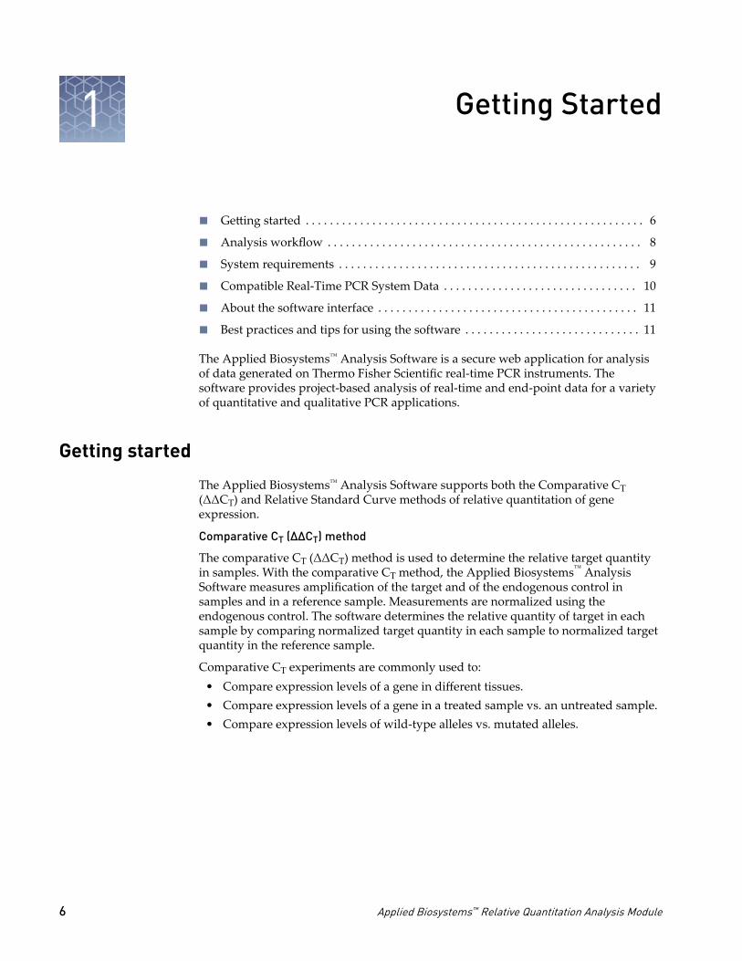
The Applied Biosystems™ Analysis Software is a secure web application for analysisof data generated on Thermo Fisher Scientific real-time PCR instruments. Thesoftware provides project-based analysis of real-time and end-point data for a varietyof quantitative and qualitative PCR applications.
Getting started
The Applied Biosystems™ Analysis Software supports both the Comparative CT(ΔΔCT) and Relative Standard Curve methods of relative quantitation of geneexpression.
Comparative CT (ΔΔCT) method
The comparative CT (ΔΔCT) method is used to determine the relative target quantityin samples. With the comparative CT method, the Applied Biosystems™ AnalysisSoftware measures amplification of the target and of the endogenous control insamples and in a reference sample. Measurements are normalized using theendogenous control. The software determines the relative quantity of target in eachsample by comparing normalized target quantity in each sample to normalized targetquantity in the reference sample.
Comparative CT experiments are commonly used to:• Compare expression levels of a gene in different tissues.• Compare expression levels of a gene in a treated sample vs. an untreated sample.• Compare expression levels of wild-type alleles vs. mutated alleles.
1
6 Applied Biosystems™ Relative Quantitation Analysis Module

The following components are required to perform a comparative Cq analysis andmust be present on all experiments added to the project:
• Sample – The sample in which the quantity of the target is unknown.• Reference sample – The sample used as the basis for relative quantitation results.
For example, in a project of drug effects on gene expression, an untreated controlwould be an appropriate reference sample. Also called calibrator.
• Endogenous control – A target or gene that should be expressed at similar levelsin all samples you are testing. The endogenous control is used to normalizefluorescence signals for the target you are quantifying. Housekeeping genes canbe used as endogenous controls.
• Replicates – The total number of identical reactions containing identical samples,components, and volumes.
• Negative controls – Wells that contain water or buffer instead of sampletemplate. No amplification of the target should occur in negative control wells.
Relative standard curve method
The Relative Standard Curve method is used to determine relative target quantity insamples using a standard curve as the basis for comparison. With the relativestandard curve method, the instrument measures the amplification of the target andendogenous control within unknown samples, a reference sample, and in a standarddilution series. During the analysis, the measurements are normalized using theendogenous control, then data from the standard dilution series are used to generatethe standard curve. Using the standard curve, the software interpolates the quantitiesof the target and endogenous control in the unknown and reference samples. For eachsample, the target quantity is normalized by the endogenous control quantity(quantity of target/quantity of endogenous control). The normalized quotient fromeach sample is divided by the quotient from the reference sample to obtain therelative quantification (fold change). The software determines the relative quantity oftarget in each sample by comparing target quantity in each sample to target quantityin the reference sample.
Relative Standard Curve experiments are commonly used to:• Compare expression levels of a gene in different tissues.• Compare expression levels of a gene in a treated sample and an untreated
sample.• Compare expression levels of wild-type alleles and mutated alleles.• Analyze the gene expression changes over time under specific treatment
conditions.
The following components are required to perform a relative standard curve analysisand must be present on all experiments added to the project:
• Sample – The tissue group that you are testing for a target gene.• Reference sample (also called a calibrator) – The sample used as the basis for
relative quantification results. For example, in a study of drug effects on geneexpression, an untreated control is an appropriate reference sample.
• Standard – A sample that contains known quantities of the target; used inquantification experiments to generate standard curves.
• Standard dilution series – A set of standards containing a range of knownquantities. The standard dilution series is prepared by serially diluting standards.
Chapter 1 Getting StartedGetting started 1
Applied Biosystems™ Relative Quantitation Analysis Module 7

• Endogenous control – A gene that is used to normalize template inputdifferences, and sample-to-sample or run-to-run variation.
• Replicates – The total number of identical reactions containing identicalcomponents and identical volumes.
• Negative Controls – Wells that contain water or buffer instead of sampletemplate. No amplification of the target should occur in the negative controlwells.
Analysis workflow
The following figure shows the general workflow for analyzing projects using theApplied Biosystems™ Analysis Software.
START
q
Create a project
q
Import and add experiment data
q
(Optional) Add and define analysis settings, samples, and targets
q
Review/edit the sample, target, and task configurations of the addedexperiments
q
Review the quality data and adjust the analysis settings if necessary
q
Review the results of the analysis and further refine the settings
q
Publish the project data
q
FINISH
Chapter 1 Getting StartedAnalysis workflow1
8 Applied Biosystems™ Relative Quantitation Analysis Module
System requirements
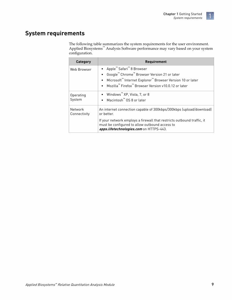
The following table summarizes the system requirements for the user environment.Applied Biosystems™ Analysis Software performance may vary based on your systemconfiguration.
Category Requirement
Web Browser • Apple™ Safari™ 8 Browser
• Google™ Chrome™ Browser Version 21 or later
• Microsoft™ Internet Explorer™ Browser Version 10 or later
• Mozilla™ Firefox™ Browser Version v10.0.12 or later
OperatingSystem
• Windows™ XP, Vista, 7, or 8
• Macintosh™ OS 8 or later
NetworkConnectivity
An internet connection capable of 300kbps/300kbps (upload/download)or better.
If your network employs a firewall that restricts outbound traffic, itmust be configured to allow outbound access toapps.lifetechnologies.com on HTTPS-443.
Chapter 1 Getting StartedSystem requirements 1
Applied Biosystems™ Relative Quantitation Analysis Module 9

Compatible Real-Time PCR System Data
The Applied Biosystems™ Analysis Software can import and analyze data generatedby any of the supported instruments listed in the following table. The softwareversions listed in the table represent only those tested for use with the AppliedBiosystems™ Software. Data generated by versions other than those listed can beimported and analyzed by the software, but are not supported by Thermo FisherScientific.
IMPORTANT! The Applied Biosystems™ Analysis Software can import and analyzedata from unsupported versions of the instrument software; however, we cannotguarantee the performance of the software or provide technical support for theanalyses.
Real-Time PCR System Supported softwareversion(s)
Fileextension
Applied Biosystems™ 7900 HT Fast Real-Time PCRSystem v2.4 or later
.sds
Applied Biosystems™ 7500 and 7500 Fast Real-Time PCR System
v1.4.1 or later
v2.0.5 or later
.eds
Applied Biosystems™ StepOne™ and StepOnePlus™
Real-Time PCR System v2.0.1, v2.1, or later
Applied Biosystems™ ViiA™ 7 Real-Time PCRSystem v1.1 or later
Applied Biosystems™ QuantStudio™ 12K Flex Real-Time PCR System v1.1.1 or later
Applied Biosystems™ QuantStudio™ 3 Real-TimePCR System
v1.0 or laterApplied Biosystems™ QuantStudio™ 5 Real-TimePCR System
Applied Biosystems™ QuantStudio™ 6 Flex Real-Time PCR System
v1.0 or laterApplied Biosystems™ QuantStudio™ 7 Flex Real-Time PCR System
Chapter 1 Getting StartedCompatible Real-Time PCR System Data1
10 Applied Biosystems™ Relative Quantitation Analysis Module
About the software interface
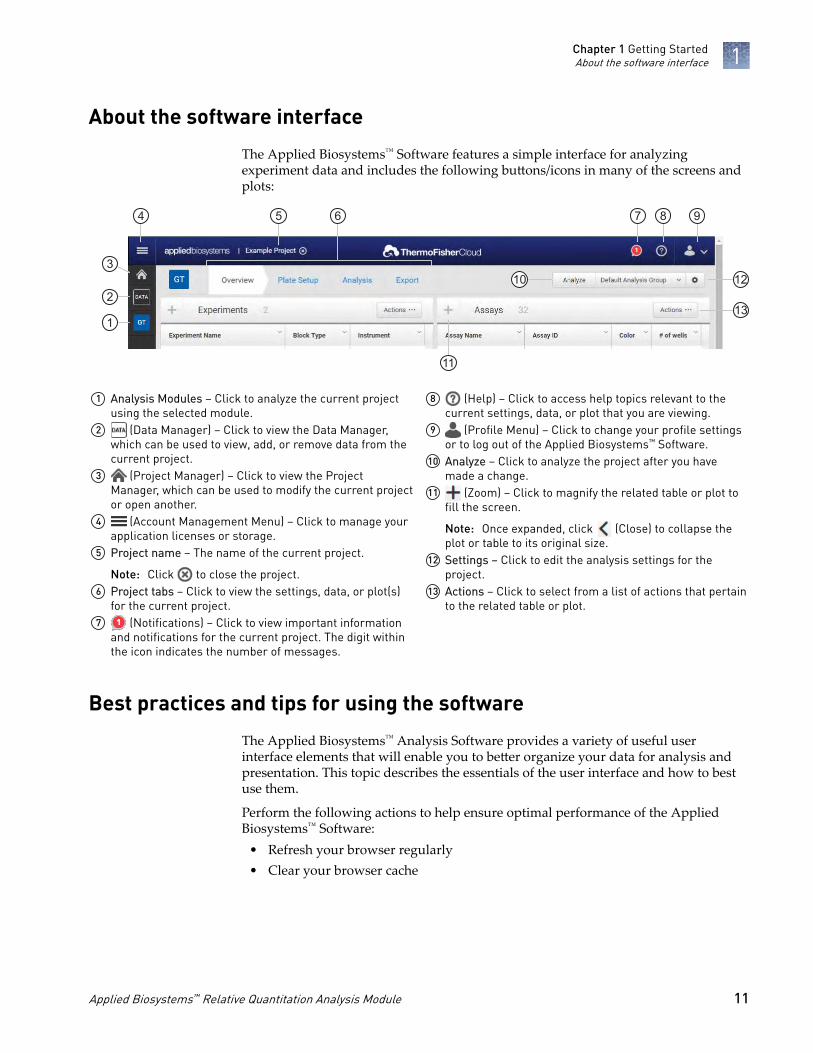
The Applied Biosystems™ Software features a simple interface for analyzingexperiment data and includes the following buttons/icons in many of the screens andplots:
3
2
1
8 97654
13
12
11
10
1 Analysis Modules – Click to analyze the current projectusing the selected module.
2 (Data Manager) – Click to view the Data Manager,which can be used to view, add, or remove data from thecurrent project.
3 (Project Manager) – Click to view the ProjectManager, which can be used to modify the current projector open another.
4 (Account Management Menu) – Click to manage yourapplication licenses or storage.
5 Project name – The name of the current project.
Note: Click to close the project.6 Project tabs – Click to view the settings, data, or plot(s)
for the current project.7 (Notifications) – Click to view important information
and notifications for the current project. The digit withinthe icon indicates the number of messages.
8 (Help) – Click to access help topics relevant to thecurrent settings, data, or plot that you are viewing.
9 (Profile Menu) – Click to change your profile settingsor to log out of the Applied Biosystems™ Software.
10 Analyze – Click to analyze the project after you havemade a change.
11 (Zoom) – Click to magnify the related table or plot tofill the screen.
Note: Once expanded, click (Close) to collapse theplot or table to its original size.
12 Settings – Click to edit the analysis settings for theproject.
13 Actions – Click to select from a list of actions that pertainto the related table or plot.
Best practices and tips for using the software
The Applied Biosystems™ Analysis Software provides a variety of useful userinterface elements that will enable you to better organize your data for analysis andpresentation. This topic describes the essentials of the user interface and how to bestuse them.
Perform the following actions to help ensure optimal performance of the AppliedBiosystems™ Software:
• Refresh your browser regularly• Clear your browser cache
Chapter 1 Getting StartedAbout the software interface 1
Applied Biosystems™ Relative Quantitation Analysis Module 11
Manage your projects andexperiment data
■ Create a project and add experiment data . . . . . . . . . . . . . . . . . . . . . . . . . . . . . . . . 12
■ Manage projects and experiment data . . . . . . . . . . . . . . . . . . . . . . . . . . . . . . . . . . . 13
■ Share experiments, folders, and projects . . . . . . . . . . . . . . . . . . . . . . . . . . . . . . . . . 14
■ About experiment data/files . . . . . . . . . . . . . . . . . . . . . . . . . . . . . . . . . . . . . . . . . . . 16
Use the Data Manager screen to add and remove experiments to and from yourproject. The screen displays all experiments associated with the current project. Youcan also use the Data Manager to upload new .eds and .sds files or view the details ofindividual experiments already added to the project.
Create a project and add experiment data
1. Click (Manage Projects) to view the Dashboard.
2. Create the project:a. Click New Project.
b. In the Create Project dialog box, enter a name for the project, select thefolder within which you want to place the project, then click OK.
Note: The project name cannot exceed 50 characters and cannot include anyof the following characters: / \ < > * ? " | : ; & % $ @ ^ ( ) !
2
12 Applied Biosystems™ Relative Quantitation Analysis Module
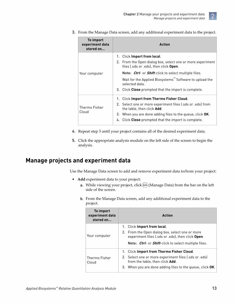
3. From the Manage Data screen, add any additional experiment data to the project.
To importexperiment data
stored on…Action
Your computer
1. Click Import from local.2. From the Open dialog box, select one or more experiment
files (.sds or .eds), then click Open.
Note: Ctrl- or Shift-click to select multiple files.
Wait for the Applied Biosystems™ Software to upload theselected data.
3. Click Close prompted that the import is complete.
Thermo FisherCloud
1. Click Import from Thermo Fisher Cloud.
2. Select one or more experiment files (.sds or .eds) fromthe table, then click Add.
3. When you are done adding files to the queue, click OK.
4. Click Close prompted that the import is complete.
4. Repeat step 3 until your project contains all of the desired experiment data.
5. Click the appropriate analysis module on the left side of the screen to begin theanalysis.
Manage projects and experiment data
Use the Manage Data screen to add and remove experiment data to/from your project:
• Add experiment data to your project:a. While viewing your project, click (Manage Data) from the bar on the left
side of the screen.
b. From the Manage Data screen, add any additional experiment data to theproject.
To importexperiment data
stored on…Action
Your computer
1. Click Import from local.2. From the Open dialog box, select one or more
experiment files (.sds or .eds), then click Open.
Note: Ctrl- or Shift-click to select multiple files.
Thermo FisherCloud
1. Click Import from Thermo Fisher Cloud.
2. Select one or more experiment files (.sds or .eds)from the table, then click Add.
3. When you are done adding files to the queue, click OK.
Chapter 2 Manage your projects and experiment dataManage projects and experiment data 2
Applied Biosystems™ Relative Quantitation Analysis Module 13
c. Wait for the Applied Biosystems™ Software to import the selected data.When you are prompted that the upload is complete, click Close.
• Delete projects, experiments, or folders:a. Select the experiments from the Files in this project table that you want to
remove.
b. From the Manage Data screen, select Actions4Delete.
c. When prompted, click OK to remove the experiment(s) from your project.
Note: Click the appropriate analysis module on the left side of the screen to return tothe analysis.
Share experiments, folders, and projects
The Applied Biosystems™ Analysis Software allows you to share any data(experiments, folders, and projects) with other users that have access to the software.Sharing data with other users grants them different access to the data depending onthe type of object shared:
• Projects – Sharing a project with other users grants them read/write access to theunlocked project.
IMPORTANT! A project is locked (preventing access) when it is open (in use) byany user with shared access to the project. For example, User A shares a projectwith two colleagues (User B and User C), User B opens the project and beginsdata analysis (the project is locked and unavailable to Users A and C) until User Bcloses the project at which time it is available again to all three users.
• Experiments – Sharing experiment files with other users grants them full accessto the data, allowing them to import the data to their own projects or downloadthe experiment data file.
• Folders – Sharing a folder with another user grants access to the contents of thefolder (projects, experiments, and subfolders).
To share projects, experiments, and subfolders with another user:
• Share an experiment, folder, or project:a. Click (Home), then click All Files to view your data.
b. From the Home Folder screen, select the check box to the left of the object(project, experiment, or folder) that you want to share, then click (displaydetails).
Chapter 2 Manage your projects and experiment dataShare experiments, folders, and projects2
14 Applied Biosystems™ Relative Quantitation Analysis Module

c. Enter the email address of the user with whom you want to share theselected object, then click .
The user is notified via email that you have shared with them and the shared itemwill appear in their Home Folder.
IMPORTANT! To share multiple files:
1. Select the desired objects (projects, experiments, and subfolders) from theHome Folder screen, then click Actions4Share.
2. In the Share Files dialog box, enter the email address of the user with whomyou want to share the selected objects, then click Share.
• Un-share a file, folder, or project:a. Click (Home), then click All Files to view your data.
b. Select the shared object, then click the display details icon.
c. In the details pane, select the Shared With tab, then click un-share adjacentto the email address of the user from which you want to remove sharingprivileges.The selected users are notified via email that you are no longer sharing thespecified file with them and the shared file(s) will no longer appear in theirHome Folder.
Chapter 2 Manage your projects and experiment dataShare experiments, folders, and projects 2
Applied Biosystems™ Relative Quantitation Analysis Module 15

About experiment data/files
The Applied Biosystems™ Analysis Software can import and analyze experiment files(.eds and .sds) that are generated by a variety of Thermo Fisher Scientific real-timeqPCR instruments. Every consumable run on a Thermo Fisher Scientific real-timeqPCR instrument requires the creation of one or more experiment files that store theassociated data. Each experiment file is a virtual representation of a specificconsumable (plate, array, or chip) that contains data for all aspects of the qPCRexperiment.
Experiment files contain the following information:• Target information and arrangement on the plate• Sample information and arrangement on the plate• Method parameters for the run
File compatibility
The Applied Biosystems™ Software can import data the following experiment fileformats generated by Applied Biosystems™ real-time qPCR instruments:
IMPORTANT! The Applied Biosystems™ Analysis Software can import and analyzedata from unsupported versions of the instrument software; however, we cannotguarantee the performance of the software or provide technical support for theanalyses.
Real-Time PCR System Supported softwareversion(s)
Fileextension
Applied Biosystems™ 7900 HT Fast Real-Time PCRSystem v2.4 or later
.sds
Applied Biosystems™ 7500 and 7500 Fast Real-Time PCR System
v1.4.1 or later
v2.0.5 or later
.eds
Applied Biosystems™ StepOne™ and StepOnePlus™
Real-Time PCR System v2.0.1, v2.1, or later
Applied Biosystems™ ViiA™ 7 Real-Time PCRSystem v1.1 or later
Applied Biosystems™ QuantStudio™ 12K Flex Real-Time PCR System v1.1.1 or later
Applied Biosystems™ QuantStudio™ 3 Real-TimePCR System
v1.0 or laterApplied Biosystems™ QuantStudio™ 5 Real-TimePCR System
Applied Biosystems™ QuantStudio™ 6 Flex Real-Time PCR System
v1.0 or laterApplied Biosystems™ QuantStudio™ 7 Flex Real-Time PCR System
Chapter 2 Manage your projects and experiment dataAbout experiment data/files2
16 Applied Biosystems™ Relative Quantitation Analysis Module
Set up the project
■ Create or edit an analysis group . . . . . . . . . . . . . . . . . . . . . . . . . . . . . . . . . . . . . . . . 17
■ Manage samples and targets . . . . . . . . . . . . . . . . . . . . . . . . . . . . . . . . . . . . . . . . . . . 20
■ Manage biological groups . . . . . . . . . . . . . . . . . . . . . . . . . . . . . . . . . . . . . . . . . . . . . 21
■ Configure the analysis settings . . . . . . . . . . . . . . . . . . . . . . . . . . . . . . . . . . . . . . . . . 22
■ Import sample information from design files . . . . . . . . . . . . . . . . . . . . . . . . . . . . . 22
■ Import target information from AIF files . . . . . . . . . . . . . . . . . . . . . . . . . . . . . . . . 23
■ Define an endogenous control for the analysis . . . . . . . . . . . . . . . . . . . . . . . . . . . . 23
After importing one or more experiments (.eds or .sds files) into your HRM project,use the Overview screen to set up the project.
Create or edit an analysis group
When a project is created, the Applied Biosystems™ Analysis Software generates thedefault analysis group from the analysis settings of the experiments added to theproject. If desired, you can create additional analysis groups to explore differentanalysis setting configurations (for example, manual versus automatic thresholding,stringent versus relaxed quality thresholds, etc).
1. From the Analysis Groups table in the Overview screen, do one of the following:• Select Actions4Add to create a new analysis group.• Select an existing group, then select Actions4Edit Analysis Settings. Go to
step 4.
2. From the Analysis Settings dialog box, enter the following information, thenclick Next.
• Group Name – Enter a name for the analysis group (up to 50 characters).• (Optional) Description – Enter a description for the analysis group (up to
256 characters).• Samples or Experiments – Select the option to determine the basis by which
the Applied Biosystems™ Software will apply the analysis group.For example, by selecting "Sample", the software allows you to apply theanalysis group to a subset of the samples within the project. Conversely, byselecting "Experiment", the software allows you to apply the analysis groupto only some of the experiments or reaction plates added to the project.
3. From the Analysis Group: Content dialog box, select the samples or experimentsto which the analysis group will apply, then click Next.
3
Applied Biosystems™ Relative Quantitation Analysis Module 17
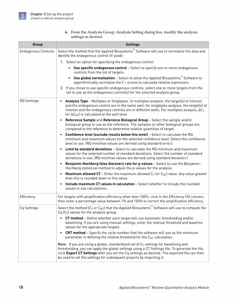
4. From the Analysis Group: Analysis Setting dialog box, modify the analysissettings as desired.
Group Settings
Endogenous Controls Select the method that the Applied Biosystems™ Software will use to normalize the data andidentify the endogenous control (if used):
1. Select an option for specifying the endogenous control:
• Use specific endogenous control – Select to specify one or more endogenouscontrols from the list of targets.
• Use global normalization – Select to allow the Applied Biosystems™ Software toalgorithmically normalize the C T scores to calculate relative expression.
2. If you chose to use specific endogenous controls, select one or more targets from thelist to use as the endogenous control(s) for the selected analysis group.
RQ Settings • Analysis Type – Multiplex or Singleplex. In multiplex analysis, the target(s) of interestand the endogenous control are in the same well; for singleplex analysis, the target(s) ofinterest and the endogenous controls are in different wells. For multiplex analysis, ∆CT(or ∆CRT) is calculated at the well level.
• Reference Sample and Reference Biological Group – Select the sample and/orbiological group to use as the reference. The samples or other biological groups arecompared to the reference to determine relative quantities of target.
• Confidence level (exclude results below this level) – Select to calculate the RQminimum and maximum values for the selected confidence level. Select the confidencelevel to use. (RQ min/max values are derived using standard error.)
• Limit by standard deviations – Select to calculate the RQ minimum and maximumvalues for the selected number of standard deviations. Select the number of standarddeviations to use. (RQ min/max values are derived using standard deviation.)
• Benjamin-Hochberg false discovery rate for p-values – Select to use the Benjamin-Hochberg statistical method to adjust the p-values for the analysis.
• Maximum allowed CT – Enter the maximum allowed CT (or CRT) value. Any value greaterthan this is rounded down to this value.
• Include maximum CT values in calculation – Select whether to include the roundedvalues in any calculations.
Efficiency For targets with amplification efficiency other than 100%, click in the Efficiency (%) column,then enter a percentage value between 1% and 150% to correct the amplification efficiency.
Cq Settings Select the method (CT or CRT) that the Applied Biosystems™ Software will use to compute theCq (CT) values for the analysis group:
• CT method – Define whether each target will use automatic thresholding and/orbaselining. If you are using manual settings, enter the manual threshold and baselinevalues for the appropriate targets.
• CRT method – Specify the cycle number that the software will use as the minimumparameter in defining the relative threshold for the CRT calculation.
Note: If you are using a global, standardized set of CT settings for baselining andthresholding, you can apply the global settings using a CT Settings file. To generate the file,click Export CT Settings after you set the Cq settings as desired. The exported file can thenbe used to set the settings for subsequent projects by importing it.
Chapter 3 Set up the projectCreate or edit an analysis group3
18 Applied Biosystems™ Relative Quantitation Analysis Module

Group Settings
Flag Settings Specify the quality measures that the Applied Biosystems™ Software will compute during theanalysis.
1. In the Use column, select the check boxes for flags you want to apply during analysis.
2. If an attribute, condition, and value are listed for a flag, you can specify the setting forapplying the flag.For example, with the default setting for the no amplification flag (NOAMP), wells areflagged if the amplification algorithm result is less than 0.1.
Note: If you choose to adjust the setting for applying a flag, make minor adjustments asyou evaluate the appropriate setting.
3. In the Reject column, select the check boxes if you want the software to reject wellswith the flag. Rejected wells are not considered for data analysis.
Inter-plate CalibratorSettings
Specify whether the Applied Biosystems™ Software will perform the analysis using an inter-plate calibrator.An IPC is a positive qPCR control, template, and assay that can be added to qPCRexperiments in a project to provide a method for normalization. When the experiments areadded for a collective analysis, a comparison of inter-plate calibrator performance can beused to account for minor variations in instrument performance.
1. Identify the target and sample combination to use as the inter-plate calibrator.
IMPORTANT! The inter-plate calibrator must be present on the reaction plates of allexperiments added to your project. Include at least three technical replicates on eachreaction plate to ensure optimal performance of the calibrator.
2. Click Add Inter-plate Calibrator Settings, then double-click the table cells in the Targetand Sample columns to select the inter-plate calibrator target and sample.
3. Repeat the previous step to add additional inter-plate calibrators to the analysissettings.
4. If desired, select Allow calculation of delta Cq across all plates in the analysis group toactivate cross-plate calculation of ∆Cq values.
Note: To remove an inter-plate calibrator setting, select the appropriate row from the table,click Delete Inter-plate Calibrator Settings, then click OK.
Chapter 3 Set up the projectCreate or edit an analysis group 3
Applied Biosystems™ Relative Quantitation Analysis Module 19

Group Settings
SC Settings If you are using a relative standard curve to perform relative quantitation, specify standardcurve settings that the Applied Biosystems™ Software will use to perform the analysis .The Relative Standard Curve is generated from a standard dilution series that is eitherpresent on the reaction plate with the unknowns or run separately on another plate. In bothcases, data from the standards are normalized to the amplification of an endogenous controland then used to generate the standard curve for quantitation. To construct the curve, youmust use the SC Settings to specify the location of the standards and select the curve fromthose detected by the software.
1. Select the location of the standard curve:
• On Plate Standard Curve – Select if the standard curve reactions are located on thesame reaction plate as the unknowns.If you want to use an on-plate standard curve to analyze other experiments,click Export and save the file.
• External Standard Curves – Select if the standard curve reactions are located on adifferent reaction plate that was run separately.
IMPORTANT! Before you can import an external standard curve, you must export itfrom the related experiment.
2. (External curve only) Click Import, then select the experiment from which you want toimport the standard curve data.
3. Select the standard curve that you want to use from the Standard Curves table.
Note: To remove an external standard curve from an analysis, select the curve from theStandard Curves table, click Delete, then click OK.
5. When done modifying the analysis settings, click Finish.
6. Click Analyze to reanalyze your project.
Manage samples and targets
The Applied Biosystems™ Analysis Software populates the Overview screen with thesamples and targets present in the experiments added to the project. If necessary, youcan add, edit, or remove the samples and targets as needed before the analysis.
• Create a new sample or target:a. From the Samples or Targets table in the Overview screen,
click Actions4Add.
b. In the New Sample/Target dialog box, enter a name for the new sample ortarget (up to 256 characters), then edit the properties of the newsample/target.
c. Click OK.
• Update an existing sample or target by editing the entry directly in the table.
Note: Alternately, select a sample or target from the table, thenselect Actions4Assign/Update.
Chapter 3 Set up the projectManage samples and targets3
20 Applied Biosystems™ Relative Quantitation Analysis Module
• Delete a sample or target:a. From the Samples or Targets table in the Overview screen, select the sample
or target of interest, then click Actions4Delete.
b. In the confirmation dialog box, click OK to delete the sample or target.
Manage biological groups
If your project uses biological replicates, assign biological replicate groups to thesamples to associate the data. The use of biological groups is optional and applicablewhen an experiment uses reactions with identical components and volumes toevaluate separate samples of the same biological source (for example, samples fromthree different mice of the same strain, or separate extractions of the same cell line ortissue sample). When an experiment uses biological replicate groups in a project, theresults are calculated by combining the results of the separate biological samples andtreating this collection as a single population (that is, as one sample).
You can use the Applied Biosystems™ Analysis Software to do the following:
• Create a new biological group:a. From the Bio Groups table in the Overview screen, select Actions4Add.
b. In the Add New Biological Group dialog box, enter a name for the newgroup (up to 256 characters), then click OK.
c. Edit the properties of the biological group directly in the BioGroups table,then click OK.
– (Optional) Select a color from the drop-down menu. (The color is shownin the box plot.)
– Enter up to a 72-character description of the biological group.
• Update an existing biological group by editing the group directly in the table.
Note: Alternately, select a biological group from the table, thenselect Actions4Update.
• Assign samples to biological groups:a. From the Samples table in the Overview screen, select one or more samples
from the list, then select Actions4Assign.
b. In the Update Sample dialog box, select the desired biological group, thenclick OK.
• Delete a biological group:a. From the Bio Groups table in the Overview screen, select the biological
group of interest, then select Actions4Delete.
b. In the confirmation dialog box, click OK to delete the group.
Chapter 3 Set up the projectManage biological groups 3
Applied Biosystems™ Relative Quantitation Analysis Module 21
Configure the analysis settings
The Applied Biosystems™ Analysis Software applies analysis settings through the useof analysis groups. You can either edit the analysis settings for the default analysisgroup or create additional groups to capture changes to the settings for latercomparison.
See “Create or edit an analysis group“ on page 17 for more information.
Import sample information from design files
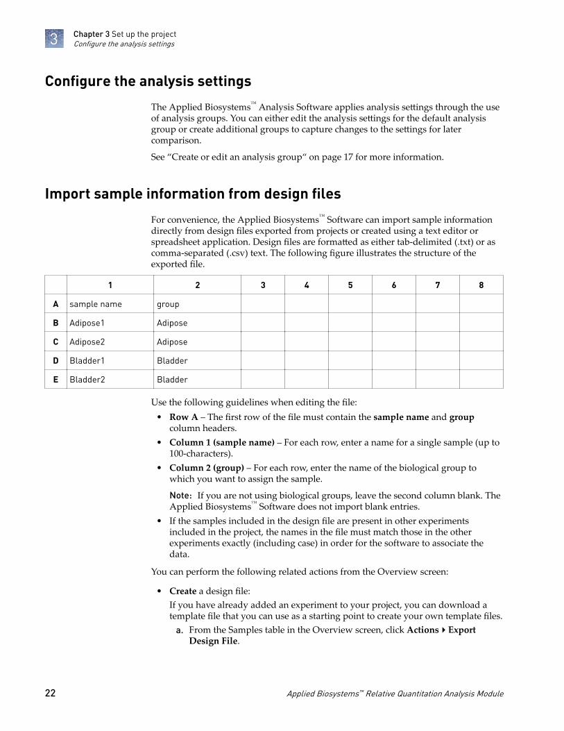
For convenience, the Applied Biosystems™ Software can import sample informationdirectly from design files exported from projects or created using a text editor orspreadsheet application. Design files are formatted as either tab-delimited (.txt) or ascomma-separated (.csv) text. The following figure illustrates the structure of theexported file.
1 2 3 4 5 6 7 8
A sample name group
B Adipose1 Adipose
C Adipose2 Adipose
D Bladder1 Bladder
E Bladder2 Bladder
Use the following guidelines when editing the file:• Row A – The first row of the file must contain the sample name and group
column headers.• Column 1 (sample name) – For each row, enter a name for a single sample (up to
100-characters).• Column 2 (group) – For each row, enter the name of the biological group to
which you want to assign the sample.
Note: If you are not using biological groups, leave the second column blank. TheApplied Biosystems™ Software does not import blank entries.
• If the samples included in the design file are present in other experimentsincluded in the project, the names in the file must match those in the otherexperiments exactly (including case) in order for the software to associate thedata.
You can perform the following related actions from the Overview screen:
• Create a design file:If you have already added an experiment to your project, you can download atemplate file that you can use as a starting point to create your own template files.
a. From the Samples table in the Overview screen, click Actions4ExportDesign File.
Chapter 3 Set up the projectConfigure the analysis settings3
22 Applied Biosystems™ Relative Quantitation Analysis Module
b. In the Export Sample Settings dialog box, select the format for the exportedfile (.txt or .csv), then click OK.
c. Using a text editor or spreadsheet application, open the sample design fileand edit it as needed.
• Import a design file:a. From the Samples table in the Overview screen, click Actions4Import
Design File.
b. Locate the sample design file with the sample information, then click Open.
If the import is successful, the sample(s) are populated to the samples in the table. If asample of the same name is already present in the project, it is overwritten with theinformation from the sample design file.
Note: Sample name matching is not case-sensitive. For instance, if the sample in theproject is "fly", then both "fly" and "Fly" in the sample design file will match.
Import target information from AIF files
For convenience, the Applied Biosystems™ Software can import target informationdirectly from assay information files (.aif), which are supplied with assaysmanufactured by Thermo Fisher Scientific. AIF are tab-delimited data files providedon a CD shipped with each assay order. The file name includes the number from thebarcode on the plate.
1. From the Targets table in the Overview screen, click Actions4Import AIF File.
2. Locate the .aif file with the target information, then click Open.
If the import is successful, the target is populated to the appropriate table. If a targetof the same target name is already present in the project, it is overwritten with theinformation from the AIF.
Note: Assay/target name matching is not case sensitive.
Define an endogenous control for the analysis
In the Applied Biosystems™ Analysis Software, the endogenous control is assignedwithin, and is specific to, each analysis group.
1. From the Analysis Groups table in the Overview screen, select an existing group,then select Actions4Edit Analysis Settings.
2. Click Endogenous Controls to view the settings.
Chapter 3 Set up the projectImport target information from AIF files 3
Applied Biosystems™ Relative Quantitation Analysis Module 23
3. Select an option for specifying the endogenous control:• Use specific endogenous control – Select to specify a specific endogenous
control from the list of targets.• Use global normalization – Select to allow the Applied Biosystems™
Software to algorithmically normalize the CT scores to calculate relativeexpression.
4. If you chose to use a specific endogenous control, select one or more targets fromthe list to use as the control(s) for the selected analysis group.
5. Click Finish.
Chapter 3 Set up the projectDefine an endogenous control for the analysis3
24 Applied Biosystems™ Relative Quantitation Analysis Module
Edit experiment properties
■ Review and edit the plate setups . . . . . . . . . . . . . . . . . . . . . . . . . . . . . . . . . . . . . . . 25
■ Apply samples and targets . . . . . . . . . . . . . . . . . . . . . . . . . . . . . . . . . . . . . . . . . . . . 26
■ Specify and assign tasks . . . . . . . . . . . . . . . . . . . . . . . . . . . . . . . . . . . . . . . . . . . . . . . 27
■ Template files . . . . . . . . . . . . . . . . . . . . . . . . . . . . . . . . . . . . . . . . . . . . . . . . . . . . . . . . 28
■ Apply plate setup information using a template file . . . . . . . . . . . . . . . . . . . . . . . 29
After populating your project with samples, targets, and controls, use the Plate Setupscreen to make changes to the plate setups of the experiments added to your project.The editor can be used to edit sample, target, task, and control assignments to correctmissing or incorrect settings.
Review and edit the plate setups
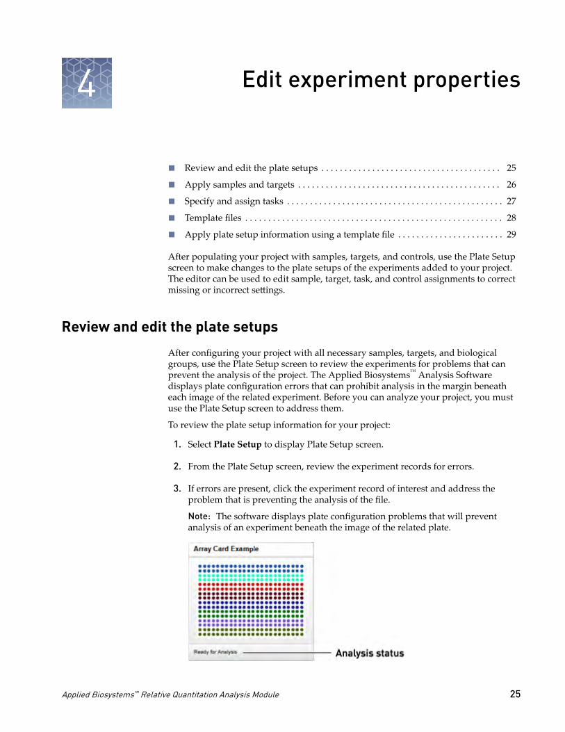
After configuring your project with all necessary samples, targets, and biologicalgroups, use the Plate Setup screen to review the experiments for problems that canprevent the analysis of the project. The Applied Biosystems™ Analysis Softwaredisplays plate configuration errors that can prohibit analysis in the margin beneatheach image of the related experiment. Before you can analyze your project, you mustuse the Plate Setup screen to address them.
To review the plate setup information for your project:
1. Select Plate Setup to display Plate Setup screen.
2. From the Plate Setup screen, review the experiment records for errors.
3. If errors are present, click the experiment record of interest and address theproblem that is preventing the analysis of the file.
Note: The software displays plate configuration problems that will preventanalysis of an experiment beneath the image of the related plate.
4
Applied Biosystems™ Relative Quantitation Analysis Module 25
Apply samples and targets
If the sample or target assignments of one or more of your experiments contain errorsor are missing, you can use the Applied Biosystems™ Analysis Software to correct theproblem prior to analysis.
Note: When reviewing a plate layout, click Actions4Clear Well Setup to remove thewell information (sample, task, and target assignments) from the selected wells in theplate grid.
1. From the Plate Setup screen, select the experiment that you want to modify.
2. (Optional) From the Edit Plate screen, click View , then select Target andSample to color the plate setup according to the element that you intend tomodify.
3. Select the wells of the plate layout to which you want to apply the target orsample.
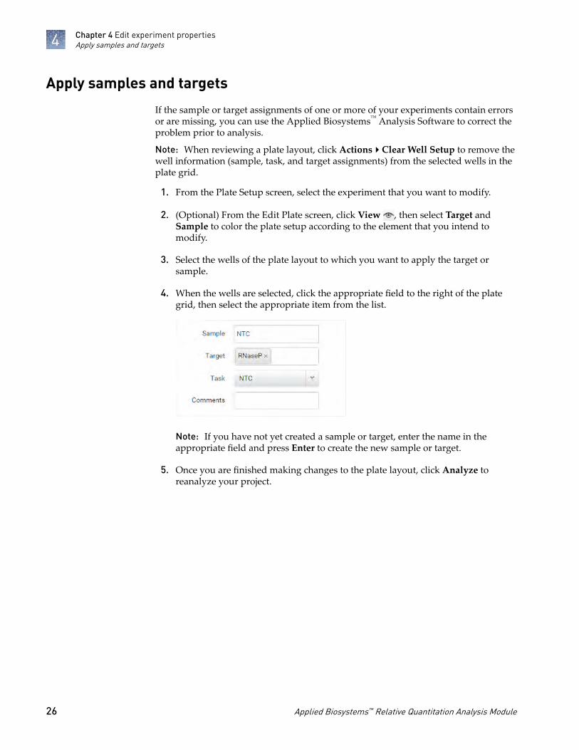
4. When the wells are selected, click the appropriate field to the right of the plategrid, then select the appropriate item from the list.
Note: If you have not yet created a sample or target, enter the name in theappropriate field and press Enter to create the new sample or target.
5. Once you are finished making changes to the plate layout, click Analyze toreanalyze your project.
Chapter 4 Edit experiment propertiesApply samples and targets4
26 Applied Biosystems™ Relative Quantitation Analysis Module

Specify and assign tasks
If the task assignments of one or more of your experiments contain errors or aremissing, you can use the Applied Biosystems™ Analysis Software to correct theproblem prior to analysis.
Note: When reviewing a plate layout, click Actions4Clear Well Setup to remove thewell information (sample, task, and target assignments) from the selected wells in theplate grid.
1. From the Plate Setup screen, select the experiment record that you want tomodify.
2. From the Edit Plate screen, click View , then select Task to color the platesetup according to task assignment.
3. Select the wells of the plate layout to which you want to apply a task.
4. When the wells are selected, click the Task menu, then select the appropriate taskfrom the list.Available tasks include:
• Unknown – The task for wells that contain a sample with unknown targetquantities.
• NTC – The task for wells that contain water or buffer instead of sample (notemplate controls). No amplification of the target should occur in negativecontrol wells.
5. Repeat steps 3 and 4 as needed.
6. Once you have completed making changes to the plate layout, click Analyze toreanalyze your project.
Chapter 4 Edit experiment propertiesSpecify and assign tasks 4
Applied Biosystems™ Relative Quantitation Analysis Module 27

Template files
The Applied Biosystems™ Analysis Software allows you to apply plate layoutinformation (such as the target, sample, and task configurations) from template filesthat you can create using a text editor or spreadsheet application. Template files arecomma-separated value (.csv) files that contain the target, sample, and taskconfigurations for a single reaction plate. You can create a template file using aspreadsheet application or a text editor, then import it using the Applied Biosystems™
Software to apply target, sample, and/or task information to experiments added to aproject.
If you have already added an experiment to your project, you can download atemplate file that you can use as a starting point to create your own template files. Thefollowing figure illustrates the general structure of the exported file.
A B C D E
Experimentdata
(do not edit):
1 * Block Type = 96-WellBlock (0.2mL)
2 * Experiment Type =Relative Quantitation
3* Instrument Type =7900HT Real-Time PCRSystem
4 * No. Of Wells = 96
Columnheadings
(do not edit):
5 Set Up Well Section Inf
6 Well Well Position Sample Name Task Target Name
Plate setupcontent (add
well data in anyorder):
7 80 G9 Testes3 UNKNOWN Hs00169663_m1
8 95 H12 Testes3 UNKNOWN Hs00608224_m1
9 14 B3 Testes1 UNKNOWN Hs00609297_m1
… … … … … …
Use the following guidelines when editing the file:• Rows 1 to 6 contain file header information that describes the experiment. In
general, you should not edit this information as it will be identical for all files thatyou use. Enter the headings exactly as shown, including upper- and lowercaseletters:
– * Block Type =– * Experiment Type =– * Instrument Type =– * No. Of Wells =– * Set Up Well Section Info =
Chapter 4 Edit experiment propertiesTemplate files4
28 Applied Biosystems™ Relative Quantitation Analysis Module

– Well– Well Position– Sample Name– Task– Target Name
• Rows 7 and below contain the plate setup information for the experiment, whereeach row contains the information for the contents of a single well on the reactionplate. As shown in the example above, the rows can occur in any order, but thelocation information (in columns 1 and 2) must be accurate.For each well the file contains the following information:
– Column A (Well) – The numerical position of the well on the plate, wherewells are numbered left to right and top to bottom. For example, on a 96-wellplate, the number of well A1 is "0" and the number of well G12 is "95".
– Column B (Well Position) – The coordinates of the well on the plate.
Note: For OpenArray™ plates, wells are identified through the combinationof the sector coordinates on the plate, and the coordinates of the well withinthe sector. For example, the position "b2d10" refers to the through-hole atposition D10 within sector B2 on the plate.
– Column C (Sample Name) – The name of the sample within the well (up to256-characters).
– Column D (Task) – The task of the sample within the well, where acceptablevalues include UNKNOWN or NTC.
– Column E (Target Name) – The name of the assay added to the well, or theidentity of the target sequence (up to 256-characters).
• If the samples and/or targets that you include in the template file are present inother experiments included in the project, the names in the file must match thosein the other experiments exactly (including case) in order for the software toassociate the data.
• When importing plate setup information from a template file, the AppliedBiosystems™ Software overwrites all existing settings with the information in thefile.
Apply plate setup information using a template file
The Applied Biosystems™ Software can import plate layout information directly fromdesign files that you can create using a text editor or spreadsheet application.
Note: For detailed information on the structure of template files, see “Templatefiles“ on page 28.
From the Plate Setup screen, you can perform the following actions:
• Download the plate setup information from an existing experiment as a templatefile:
a. Open the project that includes the experiment with the desired plate layout,then select Plate Setup.
b. From the Plate Setup screen, select the experiment record that contains thedesired plate setup.
Chapter 4 Edit experiment propertiesApply plate setup information using a template file 4
Applied Biosystems™ Relative Quantitation Analysis Module 29
c. From the Edit Plate screen, click Actions4Apply Template, then save thefile to the desired location.
• Apply plate setup information using a template file.a. Create a template file that contains the desired plate setup information.
Note: See “Template files“ on page 28 for detailed information onconstructing template files.
b. Open the project that includes the experiment to which you want to applythe template, then click Plate Setup.
c. From the Plate Setup screen, select the experiment record that you want tomodify.
d. From the Edit Plate screen, click Actions4Download Template.
e. Select the template file that contains the desired plate setup, then click Open.
If the import is successful, the sample, assay/target, and task assignments of thecurrent plate layout are overwritten with the imported settings.
IMPORTANT! The imported plate layout overrides the existing plate setup andcannot be undone once imported.
Chapter 4 Edit experiment propertiesApply plate setup information using a template file4
30 Applied Biosystems™ Relative Quantitation Analysis Module
Review the raw data
■ Review the quality data . . . . . . . . . . . . . . . . . . . . . . . . . . . . . . . . . . . . . . . . . . . . . . . 31
■ Using the Amplification Plot Histogram . . . . . . . . . . . . . . . . . . . . . . . . . . . . . . . . . 36
■ About the quality data summary . . . . . . . . . . . . . . . . . . . . . . . . . . . . . . . . . . . . . . . 36
■ Omit wells from the analysis . . . . . . . . . . . . . . . . . . . . . . . . . . . . . . . . . . . . . . . . . . . 37
After adding experiments to your project, use the Data Review screen to make a firstquality pass of your analyzed project data. The plots and features of the screen canhelp you review your project for irregular amplification and other common PCRproblems.
Review the quality data
After the Applied Biosystems™ Analysis Software processes your project, you can usethe Data Review screen to review the quality data generated by the analysis. Thesoftware provides a variety of options to review the quality data; however, thestrategy that you employ will depend on the type of quantitation you are performingand the samples/targets that you are evaluating. The following procedure describes ageneral approach to data review and provides an overview of the software features.
1. If you have not already done so, click Analyze to analyze your project.
2. In the Applied Biosystems™ Software, click Data Review to view the DataReview screen.
3. From the drop-down list at the top of the screen, choose the way that you wouldlike to organize and review the quality data:
• Targets – Groups and displays the quality data by target name.• Samples – Groups and displays the quality data by sample name.• Plates – Groups and displays the quality data by experiment/plate.
Note: The Plates view is common to all real-time instrument softwaremanufactured by Thermo Fisher Scientific.
4. Review the amplification plots for irregularities and quality flags.
Note: The Applied Biosystems™ Software displays summaries of the qualitydata in the margin beneath each amplification plot. You can view the identity ofany flag by hovering the mouse over the flag of interest.
5. If flags or irregularities are present, or you would just like to review theamplification data for a specific target, sample, or experiment, click theamplification plot of interest to zoom the display.
5
Applied Biosystems™ Relative Quantitation Analysis Module 31

6. Configure the display options for the amplification plot. Click , then selectfrom the available options:
Group Select… Description
PlotType
dRn vsCycle
Displays ΔRn as a function of cycle number, where ΔRn is themagnitude of normalized fluorescence signal generated by thereporter at each cycle during the PCR amplification. You canuse this plot to identify and examine irregular amplificationand to view threshold and baseline values for the run.
Rn vsCycle
Displays Rn as a function of cycle number, where Rn is thefluorescence signal from the reporter dye normalized to thefluorescence signal from the passive reference. You can usethis plot to identify and examine irregular amplification.
CT vsWell
Displays CT (Cq) as a function of well position, where CT is thePCR cycle number at which the fluorescence meets thethreshold in the amplification plot. You can use this plot tolocate outlying amplification (outliers).
GraphType
Linear Displays the data on a linear scale.
Log Displays the data on a logarithmic scale.
ColorType
Well Colors the data for each well according to its position on thereaction plate.
Sample Colors the data for each well according to the sample that itcontains.
FlagStatus
Colors the data for each well according to whether it generatesquality flags.
AmpStatus
Colors the data for each well according to the amplificationstatus that it is assigned.
7. If the amplification plot that you are viewing includes data from more than384 wells, use the histogram beneath the Amplification Plot to view the data ofinterest:
• Click and drag the anchor icon ( ) to the desired location in the histogramto display the curves from the 384 wells with values nearest to the positionof the icon.
• Select the heading of a column in the Well Table that contains numericalcontent (such as, Amp Score or CT/CRT without Flags) to change the x-axiscontent of the histogram.
Note: Selecting the heading of a column in the Well Table that contains less than384 data points hides the histogram. The feature is present only when the plotcontains more than 384 amplification curves.
8. If the data set that you are viewing consists of a large number of data points, usethe Outlier Wheel to organize, filter, and review the data for irregularamplification:
a. In the right-side pane of the Review Plate screen, select View By4OutlierWheel.
b. From the Sort By dropdown list, select the attribute by which you want theApplied Biosystems Software to filter the displayed data set.
Chapter 5 Review the raw dataReview the quality data5
32 Applied Biosystems™ Relative Quantitation Analysis Module

c. While viewing the data set within the Outlier Wheel, select a segment of thewheel to view the associated data within the Amplification Plot and WellTable.
Note: Click the center of the wheel to deselect the data.
d. If desired, double-click a segment of the Outlier Wheel to review the relatedsubset of the displayed data.As you select and filter the displayed data, the Applied Biosystems Softwarelists the filters that you apply at the bottom of the Outlier Wheel Plot. Toremove a filter, either click Undo to remove the last filter applied or click theX beside a desired filter to remove it.
e. At any time while reviewing your data, click Show Table to view thetabular data for the datapoints present in the Outlier Wheel Plot.
See “Outlier Wheel Plot“ on page 62 for more information on the Outlier Wheelplot.
9. Review the amplification plots as needed.When reviewing the amplification data, look for:
• Regular, characteristic amplification of all samples. If irregular amplificationis present, consider omitting the individual wells from the analysis.
• Correct baseline and threshold values. If not, consider manually adjustingthe baseline and/or threshold values in the analysis settings.
10. When ready, click Multicomponent to review the multicomponent plot asneeded.When reviewing the multicomponent plot, look for:
• Consistent fluorescence of the passive reference. The passive reference dyefluorescence level should remain relatively constant throughout the PCRprocess.
• Consistent fluorescence of the reporter dye. The reporter dye fluorescencelevel should display a flat region corresponding to the baseline, followed bya rapid rise in fluorescence as the amplification proceeds.
• Irregular fluorescence. There should not be any spikes, dips, and/or suddenchanges in the fluorescence.
• No amplification in negative control wells. There should not be anyamplification in the negative control wells.
11. View and modify the data in the Well table:
Tool Use this tool to...
Mouse/cursor
To select:
• An individual well, select the well in the Well table.
• More than one well at a time, press the Ctrl key or Shift key when you select the wells inthe Well table.
When you select wells in the Results table, the corresponding data points are selected in theamplification plot.
Chapter 5 Review the raw dataReview the quality data 5
Applied Biosystems™ Relative Quantitation Analysis Module 33

Tool Use this tool to...
Group by drop-downmenu
Select how to group the samples in the Well table. For example, if you select Target, thesamples are grouped according to the nucleic acid sequence they target.
Actions drop-downlist
Bookmark/Clear Bookmark for wells in the project.The bookmarks persist in the Data Review and Results screens, so you can easily findbookmarked wells.
Omit/UnOmit well from the analysis.After you omit or un-omit a well, click Analyze to reanalyze the project.For omitted wells, the software:
• Does not display data or tasks in the Well table.
• Does not include the omitted wells in the analysis.
For un-omitted wells, the software reassigns the tasks based on the settings in the AnalysisSettings dialog box.
Flag Details Select Show Flag Details to display the results of each quality flag in an individual column.When unselected, the table displays the results of the quality analysis in a single column.
or Expand or collapse the Well table.
12. Review the data in the Well table data.
Column Use this column to...
(Bookmark) View whether or not the well has been bookmarked.
Omit View the omission status of the related well.
CT /CRT View the CT /CRT calculated for the related well.
Amp StatusView the amplification status as determined by the software, wherepossible states are amplification, no amplification, reviewed, andundetermined.
Amp Score View the amplification score calculated for the well.
Cq Conf View the confidence value calculated by the software for the CQ (CT)for the given well.
Sample View the ID (a unique name or number) of the sample.
Target View the ID (a unique name or number) of the nucleic acidsequence targeted by the assay added to the well.
Well View the location of the well in the reaction plate. For example, P18indicates that the sample is located in row P, column 18.
PlateView the barcode of the reaction plate used to run the reaction. Ifno barcode is present, the software displays the name of theexperiment file to which the data belongs.
Baseline Start View the start and endpoints of the range of PCR cycles used asthe baseline in the calculation the CT for the related well.Baseline End
Chapter 5 Review the raw dataReview the quality data5
34 Applied Biosystems™ Relative Quantitation Analysis Module

Column Use this column to...
Task
View the task assigned to the well. A task is the function that asample performs:
• Unknown
• No template control (NTC) (control identifier)
Flags View the number of flags generated for the well.
13. When ready, click to return to the QC thumbnails.
14. Review the amplification data for specific targets, samples, or experiments asneeded.
15. Click in the toolbar to review the quality summary.Review the Quality Summary for any flags generated by the project data. Foreach quality flag, the table displays the number of times the flag was triggered bythe project data. To examine the data that triggered the flag, click the link in theName column to view the amplification data for the related target, sample, orplate.In response to the presence of quality flags, consider the following resolutions:
• Change the quality settings in the analysis group:– Adjust the sensitivity of the quality flags so that more wells or fewer
wells are flagged.– Deactivate the quality flags that triggered by the data.
• Omit individual wells from the analysis.
Chapter 5 Review the raw dataReview the quality data 5
Applied Biosystems™ Relative Quantitation Analysis Module 35

Using the Amplification Plot Histogram
When an Amplification Plot for a specific sample, target, or plate includes data formore than 384 data points, the Applied Biosystems™ Software displays a subset of thedata (shown in color) for active viewing against a background of the full dataset(shown in grey). The range of active data in the plot is controlled through a histogramof a numerical attribute associated with the well data, which is located beneath theplot (see below).
• Click and drag the anchor icon ( ) to the desired location in the histogram todisplay the curves from the 384 data points with values nearest to the position ofthe icon.
• Select the heading of a column in the Well Table that contains numerical content(such as, Amp Score or CT/CRT without Flags) to change the x-axis content of thehistogram.
Note: Selecting the heading of a column in the Well Table that contains less than384 data points hides the histogram. The feature is present only when the plotcontains more than 384 amplification curves.
About the quality data summary
The quality summary displays a table of the quality flags supported by the software.For each sample, target, or plate, the table lists the flag frequency and location for anyexperiment that is added to a project. For each quality flag, the table displays thenumber of times the flag was triggered by the project data. To examine the data thattriggered the flag, click the link in the Name column to view the amplification data forthe related target, sample, or plate.
In response to the presence of quality flags, consider the following resolutions:• Change the quality settings in the analysis group:
– Adjust the sensitivity of the quality flags so that more wells or fewer wellsare flagged.
– Deactivate the quality flags that triggered by the data.• Omit individual wells from the analysis.
Chapter 5 Review the raw dataUsing the Amplification Plot Histogram5
36 Applied Biosystems™ Relative Quantitation Analysis Module

Omit wells from the analysis
To omit the data from one or more wells that you do not want included in theanalysis:
• Select one or more wells in a plot or table, then click Actions4Omit. After thewells are omitted, click Analyze to reanalyze the project without the omittedwell(s).
IMPORTANT! You cannot omit all wells that belong to a reference sample, thatbelong to a biological group, or that serve as the endogenous control for the project.
Note: To restore an omitted well, select the well from a plot or table, thenselect Actions4UnOmit.
Chapter 5 Review the raw dataOmit wells from the analysis 5
Applied Biosystems™ Relative Quantitation Analysis Module 37

Review the analyzed data
■ Review the analyzed data and plots . . . . . . . . . . . . . . . . . . . . . . . . . . . . . . . . . . . . . 38
■ Box Plot . . . . . . . . . . . . . . . . . . . . . . . . . . . . . . . . . . . . . . . . . . . . . . . . . . . . . . . . . . . . . 42
■ Correlation Plot . . . . . . . . . . . . . . . . . . . . . . . . . . . . . . . . . . . . . . . . . . . . . . . . . . . . . . 42
■ RQ Plot . . . . . . . . . . . . . . . . . . . . . . . . . . . . . . . . . . . . . . . . . . . . . . . . . . . . . . . . . . . . . 43
■ Heatmap Plot . . . . . . . . . . . . . . . . . . . . . . . . . . . . . . . . . . . . . . . . . . . . . . . . . . . . . . . . 45
■ Volcano Plot . . . . . . . . . . . . . . . . . . . . . . . . . . . . . . . . . . . . . . . . . . . . . . . . . . . . . . . . . 46
■ Melt Curve Plot . . . . . . . . . . . . . . . . . . . . . . . . . . . . . . . . . . . . . . . . . . . . . . . . . . . . . . 48
■ Omitting wells and samples . . . . . . . . . . . . . . . . . . . . . . . . . . . . . . . . . . . . . . . . . . . 48
After reviewing the data, use the Analysis screen to review the results of the analyzedproject. The screen provides a variety of plots to help you characterize the analyzeddata and to better visualize the relationships between the calculated expression of theevaluated targets.
Review the analyzed data and plots
After you have reviewed the quality data for your project, view the results of theanalysis in the Analysis screen. As with the quality check, the following proceduredescribes a general approach to data review and provides an overview of the softwarefeatures.
1. If you have not already done so, click Analyze to analyze your project.
2. In the Applied Biosystems™ Software, click Analysis to view the Analysis screen.
3. Review the Box Plot as needed (see “Box Plot“ on page 42).a. Click View Options, then select CT vs Sample from the Plot Type drop-
down list.
b. Click the magnification factor to determine the percentage of the plotdisplayed onscreen at once.
6
38 Applied Biosystems™ Relative Quantitation Analysis Module

c. Scroll down to review the data in the Well table data.
Column Use this column to...
Sample View the ID (a unique name or number) of the sample.
BiologicalGroup
View the biological group (a unique name or number) to whichthe sample belongs.
Mean View the arithmetic average of the technical replicate CTvalues.
MinView the minimum technical replicate CT value for the testsample calculated using the confidence level set in theanalysis settings.
MaxView the maximum technical replicate CT value for the testsample calculated using the confidence level set in theanalysis settings.
Median View the median CT value for the technical replicates of thesample.
Q1
View the 1st Quartile (Q1) for the sample replicate group, whichis calculated as the numeric midpoint between the lowest andmedian CT values of the technical replicates.
Note: The 1st Quartile defines lower boundary of the inter-quartile region (IQR), which is defined as the differencebetween the 3rd and 1st quartile.
Q3View the 3rd Quartile (Q3) for the sample replicate group, whichis calculated as the numeric midpoint between the median andmaximum CT values of the technical replicates.
Note: To filter the table data, click (Filter) within any column heading,configure the rules as desired, then click Filter.
Note: If desired, you can view the quality data for any selected sample or wellby selecting the element in the plot or table and clicking View QC.
4. When ready, click to review the Correlation Plot as needed (see “CorrelationPlot“ on page 42).
a. If you are using biological groups and more than 100 samples are present inthe analysis group currently in use, select a group from the drop-down listto view the corresponding data.
b. Click View Options, then select the data arrangement that you want to view(Matrix View or Tabular View).
c. Select the type of plot that you want to display (CT or ∆CT)
5. When ready, click to review the Heatmap Plot as needed (see “HeatmapPlot“ on page 45).
a. Click View Options, then select the distance measure (Euclidean Distanceor Pearson's Correlation) from the Distance Measure drop-down menu.
b. Select the clustering method (Average Linkage, Complete Linkage, or SingleLinkage) from the Clustering Method drop-down menu.
Chapter 6 Review the analyzed dataReview the analyzed data and plots 6
Applied Biosystems™ Relative Quantitation Analysis Module 39
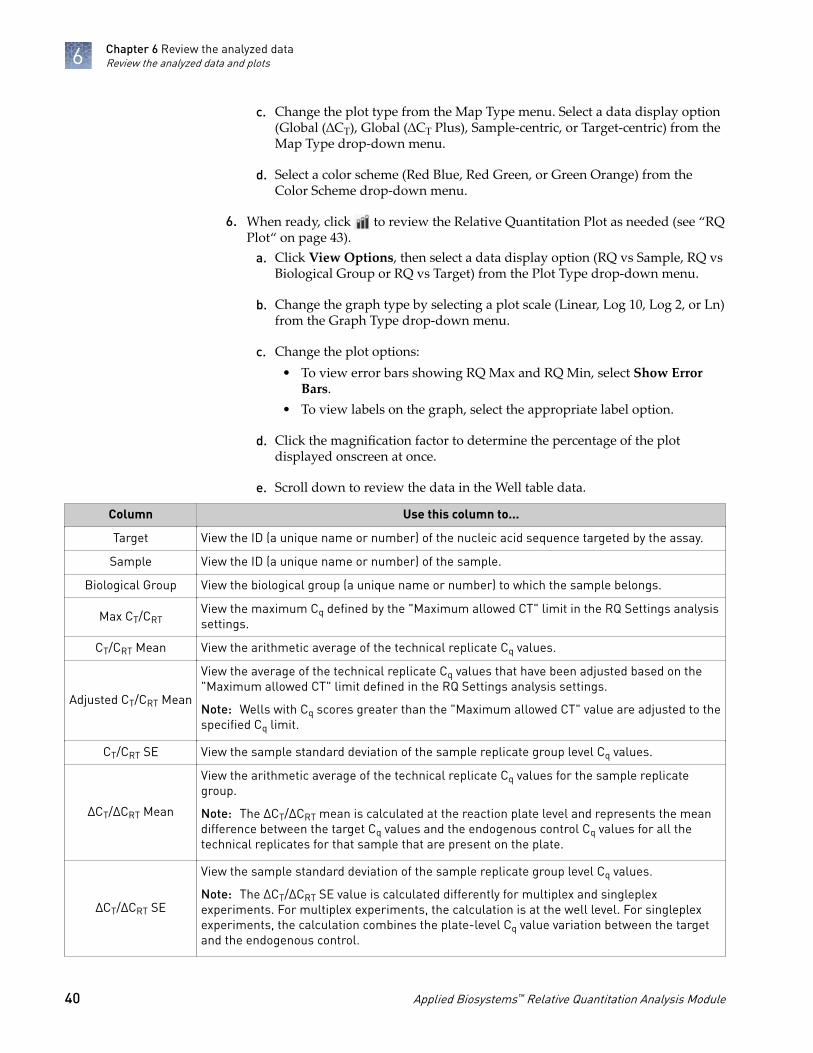
c. Change the plot type from the Map Type menu. Select a data display option(Global (∆CT), Global (∆CT Plus), Sample-centric, or Target-centric) from theMap Type drop-down menu.
d. Select a color scheme (Red Blue, Red Green, or Green Orange) from theColor Scheme drop-down menu.
6. When ready, click to review the Relative Quantitation Plot as needed (see “RQPlot“ on page 43).
a. Click View Options, then select a data display option (RQ vs Sample, RQ vsBiological Group or RQ vs Target) from the Plot Type drop-down menu.
b. Change the graph type by selecting a plot scale (Linear, Log 10, Log 2, or Ln)from the Graph Type drop-down menu.
c. Change the plot options:• To view error bars showing RQ Max and RQ Min, select Show Error
Bars.• To view labels on the graph, select the appropriate label option.
d. Click the magnification factor to determine the percentage of the plotdisplayed onscreen at once.
e. Scroll down to review the data in the Well table data.
Column Use this column to...
Target View the ID (a unique name or number) of the nucleic acid sequence targeted by the assay.
Sample View the ID (a unique name or number) of the sample.
Biological Group View the biological group (a unique name or number) to which the sample belongs.
Max CT/CRTView the maximum Cq defined by the "Maximum allowed CT" limit in the RQ Settings analysissettings.
CT/CRT Mean View the arithmetic average of the technical replicate Cq values.
Adjusted CT/CRT Mean
View the average of the technical replicate Cq values that have been adjusted based on the"Maximum allowed CT" limit defined in the RQ Settings analysis settings.
Note: Wells with Cq scores greater than the "Maximum allowed CT" value are adjusted to thespecified Cq limit.
CT/CRT SE View the sample standard deviation of the sample replicate group level Cq values.
∆CT/∆CRT Mean
View the arithmetic average of the technical replicate Cq values for the sample replicategroup.
Note: The ∆CT/∆CRT mean is calculated at the reaction plate level and represents the meandifference between the target Cq values and the endogenous control Cq values for all thetechnical replicates for that sample that are present on the plate.
∆CT/∆CRT SE
View the sample standard deviation of the sample replicate group level Cq values.
Note: The ∆CT/∆CRT SE value is calculated differently for multiplex and singleplexexperiments. For multiplex experiments, the calculation is at the well level. For singleplexexperiments, the calculation combines the plate-level Cq value variation between the targetand the endogenous control.
Chapter 6 Review the analyzed dataReview the analyzed data and plots6
40 Applied Biosystems™ Relative Quantitation Analysis Module
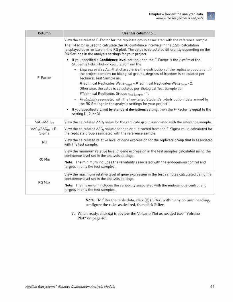
Column Use this column to...
F-Factor
View the calculated F-Factor for the replicate group associated with the reference sample.The F-Factor is used to calculate the RQ confidence intervals in the ∆∆CT calculation(displayed as error bars in the RQ plot). The value is calculated differently depending on theRQ Settings in the analysis settings for your project.
• If you specified a Confidence level setting, then the F-Factor is the t-value of theStudent's t-distribution calculated from the:
– Degrees of freedom that characterize the distribution of the replicate population. Ifthe project contains no biological groups, degrees of freedom is calculated perTechnical Test Sample as:#Technical Replicates WellsTarget + #Technical Replicates WellsEndo - 2.Otherwise, the value is calculated per Biological Test Sample as:#Technical Replicates Groups Test Sample - 1.
– Probability associated with the two-tailed Student's t-distribution (determined bythe RQ Settings in the analysis settings for your project).
• If you specified a Limit by standard deviations setting, then the F-Factor is equal to thesetting (1, 2, or 3).
∆∆CT/∆∆CRT View the calculated ΔΔCT value for the replicate group associated with the reference sample.
∆∆CT/∆∆CRT ± F-Sigma
View the calculated ΔΔCT value added to or subtracted from the F-Sigma value calculated forthe replicate group associated with the reference sample.
RQ View the calculated relative level of gene expression for the replicate group that is associatedwith the test sample.
RQ Min
View the minimum relative level of gene expression in the test samples calculated using theconfidence level set in the analysis settings.
Note: The minimum includes the variability associated with the endogenous control andtargets in only the test samples.
RQ Max
View the maximum relative level of gene expression in the test samples calculated using theconfidence level set in the analysis settings.
Note: The maximum includes the variability associated with the endogenous control andtargets in only the test samples.
Note: To filter the table data, click (Filter) within any column heading,configure the rules as desired, then click Filter.
7. When ready, click to review the Volcano Plot as needed (see “VolcanoPlot“ on page 46).
Chapter 6 Review the analyzed dataReview the analyzed data and plots 6
Applied Biosystems™ Relative Quantitation Analysis Module 41

Box Plot
The box plot displays the distribution of Cq values for each sample or for each target,making it easy to view the variation in values among biological groups.
Below the box plots is the Results Details table, showing the following information:
Column Use this column to...
Sample View the ID (a unique name or number) of the sample.
Biological Group View the biological group (a unique name or number) to which thesample belongs.
Mean View the arithmetic average of the technical replicate Cq values.
Min View the minimum technical replicate Cq value for the test samplecalculated using the confidence level set in the analysis settings.
Max View the maximum technical replicate Cq value for the test samplecalculated using the confidence level set in the analysis settings.
Median View the median Cq value for the technical replicates of the sample.
Q1
View the 1st Quartile (Q1) for the sample replicate group, which iscalculated as the numeric midpoint between the lowest and median Cqvalues of the technical replicates.
Note: The 1st Quartile defines lower boundary of the inter-quartileregion (IQR), which is defined as the difference between the 3rd and 1stquartile.
Q3View the 3rd Quartile (Q3) for the sample replicate group, which iscalculated as the numeric midpoint between the median and maximumCq values of the technical replicates.
Correlation Plot
The Correlation plots display the correlation between the target genes in one or moresamples or biological groups. There are two correlation plots: the scatter plot and thesignal correlation plot.
• The scatter plot shows the correlation of Cq for all targets for a pair of samples orbiological groups.
• The signal correlation plot shows the correlation coefficient (r) for all pairs ofsamples or biological groups in the project. The plot is color-coded based on |r|,(the absolute value of r), indicating the strength of the correlation: green indicateshighly correlated (either negative or positive) and red indicates low correlation(either negative or positive). Each cell represents a different scatter plot.
Changing the BoxPlot display
Chapter 6 Review the analyzed dataBox Plot6
42 Applied Biosystems™ Relative Quantitation Analysis Module

RQ Plot
The RQ (Relative Quantitation) Plot displays the results of the relative quantitationcalculations in the gene expression profile. Three plots are available:
• RQ vs Target – Groups the relative quantitation (RQ) values by target. Eachsample is plotted for each target. You can view the plot as the following graphtypes: linear, log10, Ln, log2.
• RQ vs Sample (present when the plot displays results by Samples) – Groups therelative quantitation (RQ) values by sample. Each target is plotted for eachsample. You can view the plot as the following graph types: linear, log10, Ln,log2.
• RQ vs BioGroup – (present when the plot displays results by Biogroups) –Groups the relative quantitation (RQ) values by biological replicate group. Eachtarget is plotted for each sample. You can view the plot as the following graphtypes: linear, log10, Ln, log2.
IMPORTANT! If one or more assay efficiencies are set less than 100%, then theApplied Biosystems™ Software performs the gene expression calculation usingequivalent Cq values, where the software adjusts the Cqs of each target proportionallyto achieve equivalent efficiency. The resulting equivalent Cqs calculated for theaffected targets reflect the values expected if the assays performed at 100% efficiency.
Below the gene expression plot is the Results Details table, showing the followinginformation:
Column Use this column to...
Target View the ID (a unique name or number) of the nucleic acid sequence targeted by the assay.
Sample View the ID (a unique name or number) of the sample.
Biological Group View the biological group (a unique name or number) to which the sample belongs.
Max CT/CRTView the maximum Cq defined by the "Maximum allowed CT" limit in the RQ Settings analysissettings.
CT/CRT Mean View the arithmetic average of the technical replicate Cq values.
Adjusted CT/CRT Mean
View the average of the technical replicate Cq values that have been adjusted based on the"Maximum allowed CT" limit defined in the RQ Settings analysis settings.
Note: Wells with Cq scores greater than the "Maximum allowed CT" value are adjusted to thespecified Cq limit.
CT/CRT SE View the sample standard deviation of the sample replicate group level Cq values.
∆CT/∆CRT Mean
View the arithmetic average of the technical replicate Cq values for the sample replicategroup.
Note: The ∆CT/∆CRT mean is calculated at the reaction plate level and represents the meandifference between the target Cq values and the endogenous control Cq values for all thetechnical replicates for that sample that are present on the plate.
Chapter 6 Review the analyzed dataRQ Plot 6
Applied Biosystems™ Relative Quantitation Analysis Module 43
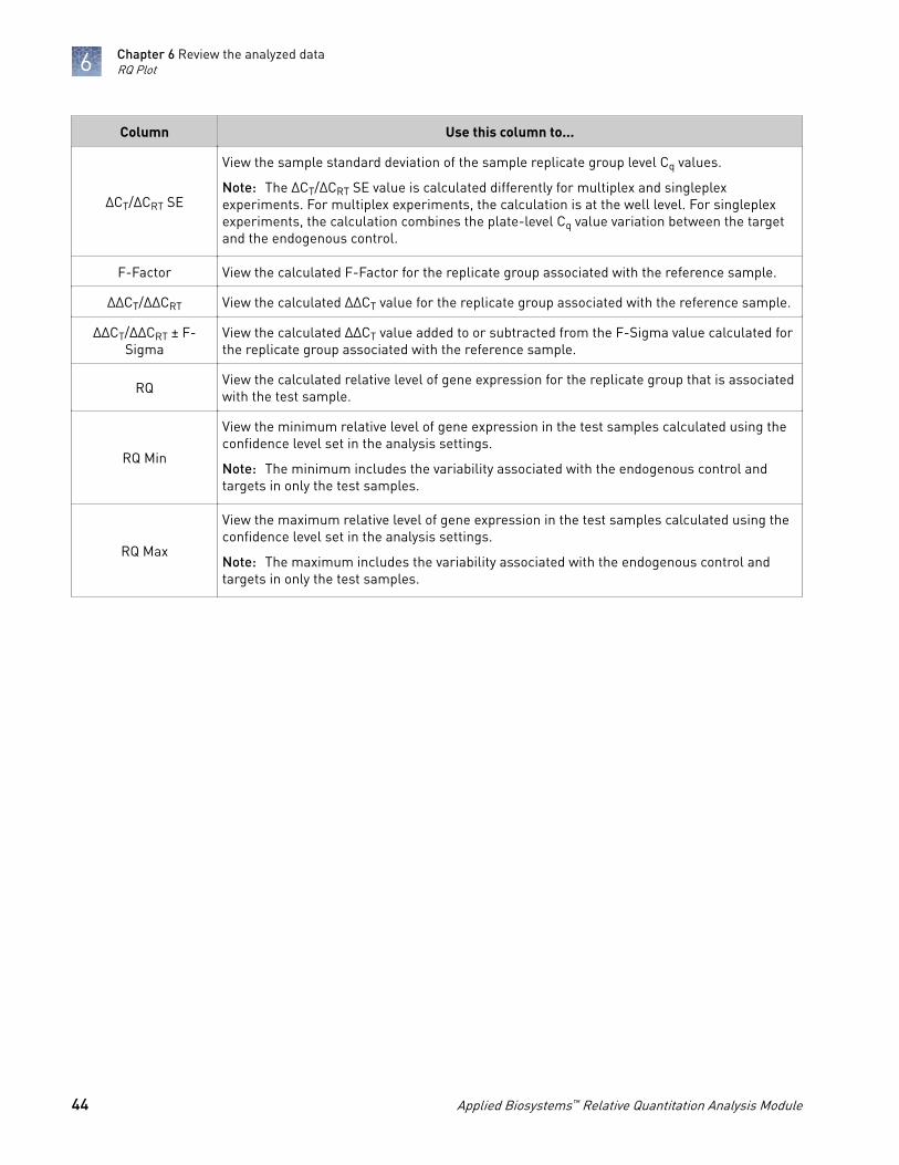
Column Use this column to...
∆CT/∆CRT SE
View the sample standard deviation of the sample replicate group level Cq values.
Note: The ∆CT/∆CRT SE value is calculated differently for multiplex and singleplexexperiments. For multiplex experiments, the calculation is at the well level. For singleplexexperiments, the calculation combines the plate-level Cq value variation between the targetand the endogenous control.
F-Factor View the calculated F-Factor for the replicate group associated with the reference sample.
∆∆CT/∆∆CRT View the calculated ΔΔCT value for the replicate group associated with the reference sample.
∆∆CT/∆∆CRT ± F-Sigma
View the calculated ΔΔCT value added to or subtracted from the F-Sigma value calculated forthe replicate group associated with the reference sample.
RQ View the calculated relative level of gene expression for the replicate group that is associatedwith the test sample.
RQ Min
View the minimum relative level of gene expression in the test samples calculated using theconfidence level set in the analysis settings.
Note: The minimum includes the variability associated with the endogenous control andtargets in only the test samples.
RQ Max
View the maximum relative level of gene expression in the test samples calculated using theconfidence level set in the analysis settings.
Note: The maximum includes the variability associated with the endogenous control andtargets in only the test samples.
Chapter 6 Review the analyzed dataRQ Plot6
44 Applied Biosystems™ Relative Quantitation Analysis Module
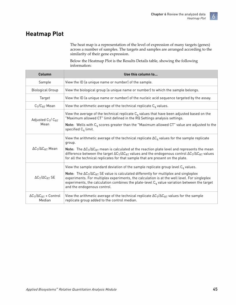
Heatmap Plot
The heat map is a representation of the level of expression of many targets (genes)across a number of samples. The targets and samples are arranged according to thesimilarity of their gene expression.
Below the Heatmap Plot is the Results Details table, showing the followinginformation:
Column Use this column to...
Sample View the ID (a unique name or number) of the sample.
Biological Group View the biological group (a unique name or number) to which the sample belongs.
Target View the ID (a unique name or number) of the nucleic acid sequence targeted by the assay.
CT/CRT Mean View the arithmetic average of the technical replicate Cq values.
Adjusted CT/ CRTMean
View the average of the technical replicate Cq values that have been adjusted based on the"Maximum allowed CT" limit defined in the RQ Settings analysis settings.
Note: Wells with Cq scores greater than the "Maximum allowed CT" value are adjusted to thespecified Cq limit.
∆CT/∆CRT Mean
View the arithmetic average of the technical replicate ∆Cq values for the sample replicategroup.
Note: The ∆CT/∆CRT mean is calculated at the reaction plate level and represents the meandifference between the target ∆CT/∆CRT values and the endogenous control ∆CT/∆CRT valuesfor all the technical replicates for that sample that are present on the plate.
∆CT/∆CRT SE
View the sample standard deviation of the sample replicate group level Cq values.
Note: The ∆CT/∆CRT SE value is calculated differently for multiplex and singleplexexperiments. For multiplex experiments, the calculation is at the well level. For singleplexexperiments, the calculation combines the plate-level Cq value variation between the targetand the endogenous control.
∆CT/∆CRT + ControlMedian
View the arithmetic average of the technical replicate ∆CT/∆CRT values for the samplereplicate group added to the control median.
Chapter 6 Review the analyzed dataHeatmap Plot 6
Applied Biosystems™ Relative Quantitation Analysis Module 45

Volcano Plot
The volcano plot displays the p-value versus the fold change for each target in abiological group, relative to the reference group. Green and red dots represent targetswith a fold change outside (greater or lesser than) the fold change boundary. Comparethe size of the fold change (x-axis) to the statistical significance level (y-axis) on thevolcano plot.
Note: You must have biological groups assigned (so that p-values can be calculated)before you can view data on the volcano plot.
IMPORTANT! If one or more assay efficiencies are set to <100%, then the AppliedBiosystems™ Software performs the gene expression calculation using equivalent Cqvalues, where the software adjusts the Cqs of each target proportionally to achieveequivalent efficiency. The resulting equivalent Cqs calculated for the affected targetsreflect the values expected if the assays performed at 100% efficiency.
Below the plot is the Results Details table, showing the following information:
Column Use this column to...
Biological Group View the biological group (a unique name or number) to which the sample belongs.
Target View the ID (a unique name or number) of the nucleic acid sequence targeted by the assay.
CT/CRT Mean View the arithmetic average of the technical replicate Cq values.
Adjusted CT/CRT Mean
View the average of the technical replicate Cq values that have been adjusted based on the"Maximum allowed CT" limit defined in the RQ Settings analysis settings.
Note: Wells with Cq scores greater than the "Maximum allowed CT" value are adjusted to thespecified Cq limit.
∆CT/∆CRT Mean
View the arithmetic average of the technical replicate Cq values for the sample replicategroup.
Note: The ∆CT/∆CRT mean is calculated at the reaction plate level and represents the meandifference between the target Cq values and the endogenous control Cq values for all thetechnical replicates for that sample that are present on the plate.
∆CT/∆CRT SE
View the sample standard deviation of the sample replicate group level Cq values.
Note: The ∆CT/∆CRT SE value is calculated differently for multiplex and singleplexexperiments. For multiplex experiments, the calculation is at the well level. For singleplexexperiments, the calculation combines the plate-level Cq value variation between the targetand the endogenous control.
∆∆CT/∆∆CRT View the calculated ΔΔCT value for the replicate group associated with the reference sample.
RQ View the calculated relative level of gene expression for the replicate group that is associatedwith the test sample.
RQ Min
View the minimum relative level of gene expression in the test samples calculated using theconfidence level set in the analysis settings.
Note: The minimum includes the variability associated with the endogenous control andtargets in only the test samples.
Chapter 6 Review the analyzed dataVolcano Plot6
46 Applied Biosystems™ Relative Quantitation Analysis Module
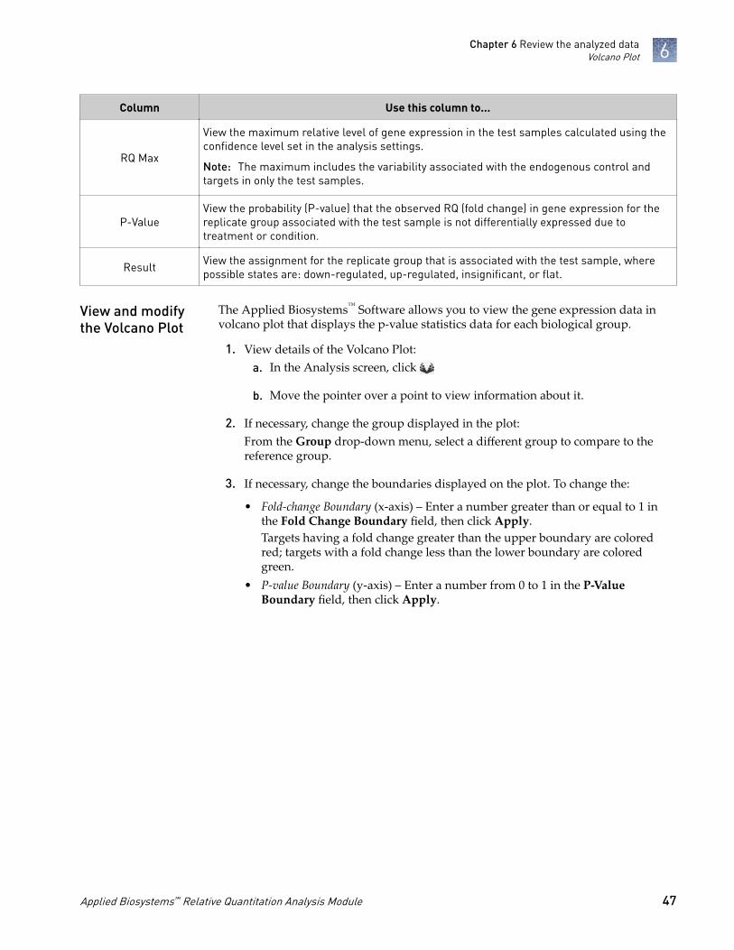
Column Use this column to...
RQ Max
View the maximum relative level of gene expression in the test samples calculated using theconfidence level set in the analysis settings.
Note: The maximum includes the variability associated with the endogenous control andtargets in only the test samples.
P-ValueView the probability (P-value) that the observed RQ (fold change) in gene expression for thereplicate group associated with the test sample is not differentially expressed due totreatment or condition.
Result View the assignment for the replicate group that is associated with the test sample, wherepossible states are: down-regulated, up-regulated, insignificant, or flat.
The Applied Biosystems™ Software allows you to view the gene expression data involcano plot that displays the p-value statistics data for each biological group.
1. View details of the Volcano Plot:a. In the Analysis screen, click
b. Move the pointer over a point to view information about it.
2. If necessary, change the group displayed in the plot:From the Group drop-down menu, select a different group to compare to thereference group.
3. If necessary, change the boundaries displayed on the plot. To change the:
• Fold-change Boundary (x-axis) – Enter a number greater than or equal to 1 inthe Fold Change Boundary field, then click Apply.Targets having a fold change greater than the upper boundary are coloredred; targets with a fold change less than the lower boundary are coloredgreen.
• P-value Boundary (y-axis) – Enter a number from 0 to 1 in the P-ValueBoundary field, then click Apply.
View and modifythe Volcano Plot
Chapter 6 Review the analyzed dataVolcano Plot 6
Applied Biosystems™ Relative Quantitation Analysis Module 47

Melt Curve Plot
The melt curve plot (also called a dissociation curve plot) displays data collectedduring a melt curve stage. Peaks in the melt curve can indicate the meltingtemperature (Tm) of a target or can identify nonspecific PCR amplification. Thesoftware displays the melt curve plot only for those experiments with a PCR methodthat includes a melt curve stage (a gradual temperature ramp configured for datacollection).
Two views are available:• Normalized reporter (Rn) vs. temperature — The normalized reporter view
visualizes the rise in fluorescence throughout the temperature ramp. Thenormalized reporter (Rn), displayed on the y-axis, is calculated as thefluorescence signal from the reporter dye normalized to the fluorescence signal ofthe passive reference.
• Derivative reporter (−Rn′) vs. temperature — The derivative reporter viewallows you to visualize the maximum rate of change in fluorescence during thetemperature ramp. The derivative reporter, displayed on the y-axis, is calculatedas the negative first derivative of the normalized fluorescence (Rn) generated bythe reporter during PCR amplification.
Omitting wells and samples
You may omit wells from analysis if you do not want to consider data generated bythe well.
1. Select one or more wells to omit from analysis.
2. Omit the selected wells:
• Well Table tab - Select the wells, then select Actions4Omit.• Plate Layout tab - Select the wells, then click Omit.
3. Click Analyze to reanalyze the data without the omitted wells.
IMPORTANT! You cannot omit all wells that belong to a reference sample, thatbelong to a biological group, or that serve as the endogenous control for a project.
Chapter 6 Review the analyzed dataMelt Curve Plot6
48 Applied Biosystems™ Relative Quantitation Analysis Module
Export the results
■ Export the analyzed data from a project . . . . . . . . . . . . . . . . . . . . . . . . . . . . . . . . . 49
■ Export project data as a slide presentation . . . . . . . . . . . . . . . . . . . . . . . . . . . . . . . 50
■ Export plots for presentation and publication . . . . . . . . . . . . . . . . . . . . . . . . . . . . 51
■ Export data for use in other projects . . . . . . . . . . . . . . . . . . . . . . . . . . . . . . . . . . . . 52
After you are finished analyzing your project, you can use the Applied Biosystems™
Analysis Software to publish the project data.
Export the analyzed data from a project
The Applied Biosystems™ Analysis Software allows you to export project data ascomma-separated or tab-delimited text, which can be imported by most spreadsheetapplications for further analysis or presentation.
1. From the main menu of the project that contains data to export, click Export.
2. From the Export screen, click , then enter the following information:a. Enter a name for the exported report in the Name field.
Note: Naming the report will allow you to repeat the export if you need todo so again.
b. Select the file type for the exported data:• .txt - To export data to a tab-delimited text file.• .csv - To export data to a comma-separated text file.
c. (CSV and TXT exports only) Select the check boxes for the data that you wantto export.
• Biological Group Results - Exports gene expression analysis resultsorganized and analyzed by biological group.
• Sample Results - Exports gene expression analysis results organizedand analyzed by individual samples.
• Well Results - Exports gene expression analysis results for theindividuals wells of every reaction plate used in the analysis.
• Amplification Data - Exports amplification results for each well in theproject, such as cycle numbers, and Rn or ΔRn values.
7
Applied Biosystems™ Relative Quantitation Analysis Module 49

• Volcano Plot Data - Exports gene expression data used to generate theVolcano Plot, including Fold Change, P-Value, Fold Change Boundary,P-Value Boundary, and the Result.
• Targets/Samples/Plates QC (with flags) - Exports a summary of thequality metrics (flags) generated by the data analysis. The option allowsyou to selectively export the quality data organized by target, sample,or plate.
3. If you want to customize the export to include specific data, clickActions4Customize, then select the data columns that you want to export fromeach selected tables.
4. From the Export Details screen, select the fields from the data tables to include inthe exported file, then click Start Export.After starting the export, wait for the Applied Biosystems™ Analysis Software togenerate the report. The export is complete when the Status column of theexported report displays "Download".After generating the data export, the Applied Biosystems™ Software displays thepackage as a row in the Export History table.
5. (Optional) Click the entry in the Comments column, then enter any additionalinformation for the exported report.
6. Click Download, select the location for the exported data file, then click Save.
Once generated, a data export package remains in the Export History indefinitely oruntil you remove it. To delete a package, select an export package from the table, thenclick Actions and select Delete File(s).
Export project data as a slide presentation
The Applied Biosystems™ Analysis Software allows you to export your project data asa Microsoft™ PowerPoint® slide presentation. The exported file summarizes the projectdata and saves the exported file in a generic template that you can override byimporting a Microsoft™ PowerPoint® template file.
1. From the main menu of the project that contains data to export, click Export.
2. From the Export screen, click , then enter the following information:a. Enter a name for the exported report in the Name field.
Note: Naming the report will allow you to repeat the export if you need todo so again.
b. From the File type menu, select .pptx.
Chapter 7 Export the resultsExport project data as a slide presentation7
50 Applied Biosystems™ Relative Quantitation Analysis Module

3. From the Export Details screen, select the fields from the data tables to include inthe exported file, then click Start Export.After starting the export, wait for the Applied Biosystems™ Analysis Software togenerate the report. The export is complete when the Status column of theexported report displays "Download".After generating the data export, the Applied Biosystems™ Software displays thepackage as a row in the Export History table.
4. (Optional) Click the entry in the Comments column, then enter any additionalinformation for the exported report.
5. Click Download, select the location for the exported data file, then click Save.
Once generated, a data export package remains in the Export History indefinitely oruntil you remove it. To delete a package, select an export package from the table, thenclick Actions and select Delete File(s).
You can use the Microsoft™ PowerPoint® Application to reformat the exported slidepresentation. For more information on applying a theme or template to yourpresentation, refer to the Microsoft™ PowerPoint® Help.
Export plots for presentation and publication
The Applied Biosystems™ Analysis Software allows you to export any plot as aPortable Network Graphics (.png) or Joint Photographic Expert Group (.jpg) file,which can be imported by most spreadsheet and desktop publishing software forpresentation.
1. When viewing a plot, click (Save as image) or select Actions4Save as Image.
2. Save the image.a. Click the File Name field, then enter a name for the exported graphics file.
b. Select the appropriate file format (.png or .jpg).
Chapter 7 Export the resultsExport plots for presentation and publication 7
Applied Biosystems™ Relative Quantitation Analysis Module 51
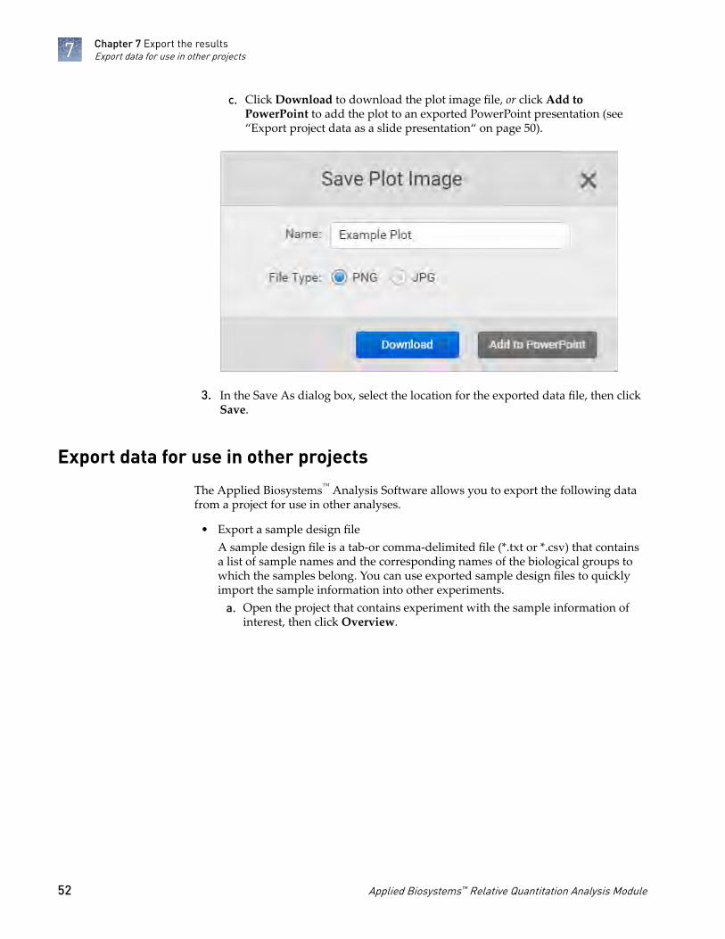
c. Click Download to download the plot image file, or click Add toPowerPoint to add the plot to an exported PowerPoint presentation (see “Export project data as a slide presentation“ on page 50).
3. In the Save As dialog box, select the location for the exported data file, then clickSave.
Export data for use in other projects
The Applied Biosystems™ Analysis Software allows you to export the following datafrom a project for use in other analyses.
• Export a sample design fileA sample design file is a tab-or comma-delimited file (*.txt or *.csv) that containsa list of sample names and the corresponding names of the biological groups towhich the samples belong. You can use exported sample design files to quicklyimport the sample information into other experiments.
a. Open the project that contains experiment with the sample information ofinterest, then click Overview.
Chapter 7 Export the resultsExport data for use in other projects7
52 Applied Biosystems™ Relative Quantitation Analysis Module

b. From the Samples table in the Overview screen, click Actions4ExportDesign File.
c. In the Export Sample Settings dialog box, select the format for the exportedfile (.txt or .csv), then click OK.
d. Select the location and name for the exported file, then click Save.
• Export a template fileTemplate files contain plate layout information (target, sample, and taskconfigurations) that you can use to easily set up experiments added to yourprojects. The Applied Biosystems™ Software allows you to export template filesfrom existing experiments or to create them using a text editor or spreadsheetapplication.
a. Open the project that includes the desired experiment, then select PlateSetup.
b. From the Plate Setup screen, select the experiment record that contains theplate setup information of interest.
c. From the Edit Plate screen, click Actions4Download Template, then savethe file to the desired location.
• Export the amplification efficiency settingsAmplification efficiency files associate targets with the specific amplificationefficiencies of the corresponding assays. Once exported, you can use the file toimport the settings to other projects (especially useful for projects involving largenumbers of targets).
a. Open the project that includes the analysis settings with the desiredefficiency data, then select Overview.
Chapter 7 Export the resultsExport data for use in other projects 7
Applied Biosystems™ Relative Quantitation Analysis Module 53

b. From the Overview screen, select the analysis group that contains theefficiency data, then click Edit Analysis Settings.
c. From the Analysis Settings dialog box, click Efficiency to view the assayefficiency settings, then click Export.
d. In the Export Sample Settings dialog box, select the format for the exportedfile (.txt or .csv), then click OK.
e. Select the location and name for the exported file, then click Save.
• Export the CT settingsThe CT settings file associates targets with specific methods for calculatingbaseline and threshold values (manual or automatic). Once exported, you can usethe file to import the settings to other projects (especially useful for projectsinvolving large numbers of targets).
a. Open the project that includes the analysis settings with the desired CTsettings, then select Overview.
Chapter 7 Export the resultsExport data for use in other projects7
54 Applied Biosystems™ Relative Quantitation Analysis Module

b. From the Overview screen, select the analysis group that contains the CTsettings, then select Action4Edit Analysis Settings.
c. From the Analysis Settings dialog box, click Cq Settings to view the Cqsettings, then click Export CT Settings.
d. In the Export CT Settings dialog box, select the format for the exported file(.txt or .csv), then click OK.
e. Select the location and name for the exported file, then click Save.
Chapter 7 Export the resultsExport data for use in other projects 7
Applied Biosystems™ Relative Quantitation Analysis Module 55
Screens and plots
■ Amplification Plot . . . . . . . . . . . . . . . . . . . . . . . . . . . . . . . . . . . . . . . . . . . . . . . . . . . . 57
■ Box Plot . . . . . . . . . . . . . . . . . . . . . . . . . . . . . . . . . . . . . . . . . . . . . . . . . . . . . . . . . . . . . 58
■ Correlation Plot . . . . . . . . . . . . . . . . . . . . . . . . . . . . . . . . . . . . . . . . . . . . . . . . . . . . . . 59
■ Heatmap Plot . . . . . . . . . . . . . . . . . . . . . . . . . . . . . . . . . . . . . . . . . . . . . . . . . . . . . . . . 59
■ Melt Curve Plot . . . . . . . . . . . . . . . . . . . . . . . . . . . . . . . . . . . . . . . . . . . . . . . . . . . . . . 60
■ Multicomponent Plot . . . . . . . . . . . . . . . . . . . . . . . . . . . . . . . . . . . . . . . . . . . . . . . . . 61
■ Outlier Wheel Plot . . . . . . . . . . . . . . . . . . . . . . . . . . . . . . . . . . . . . . . . . . . . . . . . . . . . 62
■ RQ Plot . . . . . . . . . . . . . . . . . . . . . . . . . . . . . . . . . . . . . . . . . . . . . . . . . . . . . . . . . . . . . 63
■ Volcano Plot . . . . . . . . . . . . . . . . . . . . . . . . . . . . . . . . . . . . . . . . . . . . . . . . . . . . . . . . . 65
■ Well Table . . . . . . . . . . . . . . . . . . . . . . . . . . . . . . . . . . . . . . . . . . . . . . . . . . . . . . . . . . . 66
The Applied Biosystems™ Analysis Software provides the following screens and plotsthat can be used to edit and visualize experiment setups and results that have beenadded to your project.
8
56 Applied Biosystems™ Relative Quantitation Analysis Module
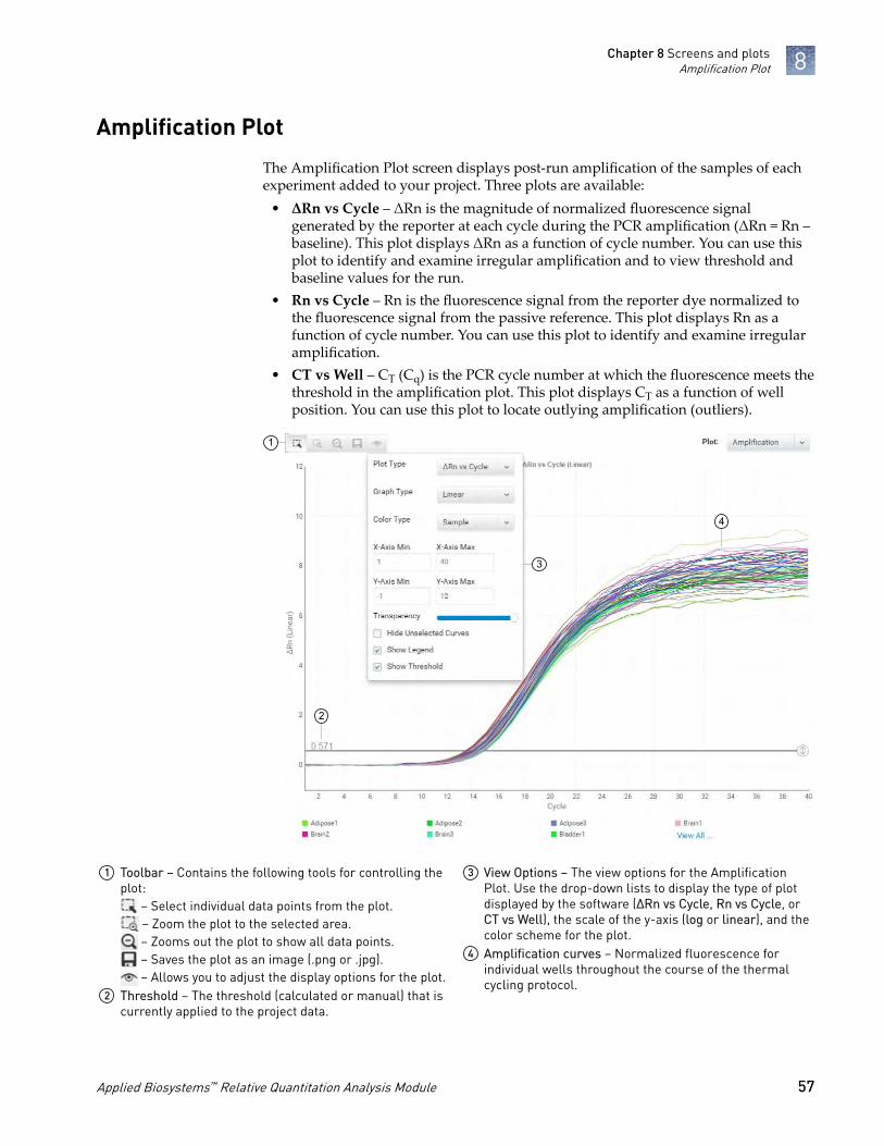
Amplification Plot
The Amplification Plot screen displays post-run amplification of the samples of eachexperiment added to your project. Three plots are available:
• ΔRn vs Cycle – ΔRn is the magnitude of normalized fluorescence signalgenerated by the reporter at each cycle during the PCR amplification (ΔRn = Rn –baseline). This plot displays ΔRn as a function of cycle number. You can use thisplot to identify and examine irregular amplification and to view threshold andbaseline values for the run.
• Rn vs Cycle – Rn is the fluorescence signal from the reporter dye normalized tothe fluorescence signal from the passive reference. This plot displays Rn as afunction of cycle number. You can use this plot to identify and examine irregularamplification.
• CT vs Well – CT (Cq) is the PCR cycle number at which the fluorescence meets thethreshold in the amplification plot. This plot displays CT as a function of wellposition. You can use this plot to locate outlying amplification (outliers).
2
3
1
4
1 Toolbar – Contains the following tools for controlling theplot:
– Select individual data points from the plot. – Zoom the plot to the selected area. – Zooms out the plot to show all data points. – Saves the plot as an image (.png or .jpg). – Allows you to adjust the display options for the plot.
2 Threshold – The threshold (calculated or manual) that iscurrently applied to the project data.
3 View Options – The view options for the AmplificationPlot. Use the drop-down lists to display the type of plotdisplayed by the software (ΔRn vs Cycle, Rn vs Cycle, orCT vs Well), the scale of the y-axis (log or linear), and thecolor scheme for the plot.
4 Amplification curves – Normalized fluorescence forindividual wells throughout the course of the thermalcycling protocol.
Chapter 8 Screens and plotsAmplification Plot 8
Applied Biosystems™ Relative Quantitation Analysis Module 57

Note: When the Amplification Plot displays a large data set, the AppliedBiosystems™ Software alters the appearance of curves to better identify them:· Inactive data – Displayed using solid, grey curves· Omitted data – Wells omitted automatically/manually are displayed using Long-
dashed, grey curves ( — — — )· Unselected data – Wells not part of the current selection are displayed using short-
dashed, grey curves ( - - - - - - )
Viewing large data sets
When an Amplification Plot for a specific sample, target, or plate includes data formore than 384 data points, the Applied Biosystems™ Software displays a subset of thedata (shown in color) for active viewing against a background of the full data set(shown in grey). The range of active data in the Amplification Plot is controlledthrough a histogram, located beneath the plot, which displays the well data for theexperiment tabulated by an associated numerical attribute (such as Amp Score orCT/CRT without Flags).
The position of the anchor icon ( ) in the histogram controls the range of active datadisplayed by the Amplification Plot, where the software displays the curves from the384 data points with values nearest to the position of the icon. To change the range ofactive data, click and drag the icon to view the data nearest the desired location.
Note: Alternatively, click / below the Well Table to advance the active data rangedisplayed by the Amplification Plot.
The content of the histogram is determined by the table heading selected in the WellTable. By default, the histogram tabulates data by Amp Score as shown above. Tochange the data displayed on the x-axis of the histogram, select the heading of acolumn in the Well Table that contains numerical content (such as, Amp Score orCT/CRT without Flags).
Note: Selecting the heading of a column in the Well Table that contains less than 384data points hides the histogram. The feature is present only when the plot containsmore than 384 amplification curves.
Box Plot
The box plot displays the distribution of Cq values for each sample or for each target,making it easy to view the variation in values among biological groups.
Below the box plots is the Results Details table, showing the following information:
Column Use this column to...
Sample View the ID (a unique name or number) of the sample.
Biological Group View the biological group (a unique name or number) to which thesample belongs.
Mean View the arithmetic average of the technical replicate Cq values.
Min View the minimum technical replicate Cq value for the test samplecalculated using the confidence level set in the analysis settings.
Chapter 8 Screens and plotsBox Plot8
58 Applied Biosystems™ Relative Quantitation Analysis Module

Column Use this column to...
Max View the maximum technical replicate Cq value for the test samplecalculated using the confidence level set in the analysis settings.
Median View the median Cq value for the technical replicates of the sample.
Q1
View the 1st Quartile (Q1) for the sample replicate group, which iscalculated as the numeric midpoint between the lowest and median Cqvalues of the technical replicates.
Note: The 1st Quartile defines lower boundary of the inter-quartileregion (IQR), which is defined as the difference between the 3rd and 1stquartile.
Q3View the 3rd Quartile (Q3) for the sample replicate group, which iscalculated as the numeric midpoint between the median and maximumCq values of the technical replicates.
Correlation Plot
The Correlation plots display the correlation between the target genes in one or moresamples or biological groups. There are two correlation plots: the scatter plot and thesignal correlation plot.
• The scatter plot shows the correlation of Cq for all targets for a pair of samples orbiological groups.
• The signal correlation plot shows the correlation coefficient (r) for all pairs ofsamples or biological groups in the project. The plot is color-coded based on |r|,(the absolute value of r), indicating the strength of the correlation: green indicateshighly correlated (either negative or positive) and red indicates low correlation(either negative or positive). Each cell represents a different scatter plot.
Heatmap Plot
The heat map is a representation of the level of expression of many targets (genes)across a number of samples. The targets and samples are arranged according to thesimilarity of their gene expression.
Below the Heatmap Plot is the Results Details table, showing the followinginformation:
Column Use this column to...
Sample View the ID (a unique name or number) of the sample.
Biological Group View the biological group (a unique name or number) to which the sample belongs.
Target View the ID (a unique name or number) of the nucleic acid sequence targeted by the assay.
CT/CRT Mean View the arithmetic average of the technical replicate Cq values.
Chapter 8 Screens and plotsCorrelation Plot 8
Applied Biosystems™ Relative Quantitation Analysis Module 59

Column Use this column to...
Adjusted CT/ CRTMean
View the average of the technical replicate Cq values that have been adjusted based on the"Maximum allowed CT" limit defined in the RQ Settings analysis settings.
Note: Wells with Cq scores greater than the "Maximum allowed CT" value are adjusted to thespecified Cq limit.
∆CT/∆CRT Mean
View the arithmetic average of the technical replicate ∆Cq values for the sample replicategroup.
Note: The ∆CT/∆CRT mean is calculated at the reaction plate level and represents the meandifference between the target ∆CT/∆CRT values and the endogenous control ∆CT/∆CRT valuesfor all the technical replicates for that sample that are present on the plate.
∆CT/∆CRT SE
View the sample standard deviation of the sample replicate group level Cq values.
Note: The ∆CT/∆CRT SE value is calculated differently for multiplex and singleplexexperiments. For multiplex experiments, the calculation is at the well level. For singleplexexperiments, the calculation combines the plate-level Cq value variation between the targetand the endogenous control.
∆CT/∆CRT + ControlMedian
View the arithmetic average of the technical replicate ∆CT/∆CRT values for the samplereplicate group added to the control median.
Melt Curve Plot
The melt curve plot (also called a dissociation curve plot) displays data collectedduring a melt curve stage. Peaks in the melt curve can indicate the meltingtemperature (Tm) of a target or can identify nonspecific PCR amplification. Thesoftware displays the melt curve plot only for those experiments with a PCR methodthat includes a melt curve stage (a gradual temperature ramp configured for datacollection).
Two views are available:• Normalized reporter (Rn) vs. temperature — The normalized reporter view
visualizes the rise in fluorescence throughout the temperature ramp. Thenormalized reporter (Rn), displayed on the y-axis, is calculated as thefluorescence signal from the reporter dye normalized to the fluorescence signal ofthe passive reference.
• Derivative reporter (−Rn′) vs. temperature — The derivative reporter viewallows you to visualize the maximum rate of change in fluorescence during thetemperature ramp. The derivative reporter, displayed on the y-axis, is calculatedas the negative first derivative of the normalized fluorescence (Rn) generated bythe reporter during PCR amplification.
Chapter 8 Screens and plotsMelt Curve Plot8
60 Applied Biosystems™ Relative Quantitation Analysis Module

Multicomponent Plot
The Multicomponent Plot is a plot of the complete spectral contribution of each dyefor the selected well(s) over the duration of the PCR run.
2
3
1
4
1 Toolbar – Contains the following tools for controlling theplot:
– Select individual data points from the plot. – Allows you to click and manually move the position
of the plot. – Zoom the plot to the selected area. – Zooms out the plot to show all data points. – Saves the plot as an image (.png or .jpg).
– Allows you to adjust the display options for the plot.2 Target/Sample drop-down list – Selects the data from the
target or sample data displayed by the plot.3 Normalized fluorescence – Displays the normalized
fluorescence for all wells throughout the duration of thethermal cycling protocol.
4 Legend – Fluorescent dyes present in the analyzed data.
When you analyze your own experiment, confirm the following:• The passive reference dye fluorescence level should remain relatively constant
throughout the PCR process.• The reporter dye fluorescence level should display a flat region corresponding to
the baseline, followed by a rapid rise in fluorescence as the amplificationproceeds.
• There should not be any spikes, dips, and/or sudden changes in the fluorescentsignal.
• There should not be any amplification in negative control wells.
Chapter 8 Screens and plotsMulticomponent Plot 8
Applied Biosystems™ Relative Quantitation Analysis Module 61

Outlier Wheel Plot
The Outlier Wheel is a data review tool that can greatly simplify the quality controlreview of very large data sets, especially data generated by OpenArray experiments.When a sample, target, or plate data set consists of thousands of data points, you canuse the Outlier Wheel to organize and review the data set for irregular amplification.
The Outlier Wheel simplifies the review process by visualizing the amplification dataof a given data set in a circular format, where each amplification curve in the set isrepresented as a colored line extending from a central axis. As shown in the followingfigure, each line is broken into colored segments that map to regions of theamplification curve, where:
• Segment length indicates the increase in normalized fluorescence (Rn) at a givenPCR cycle.
• Segment color indicates the PCR cycle number at which signal was collected.
In the example below, the amplification curve exhibits little growth in Rn during cycle1 (shown in cyan). Therefore, the projection of that section of the curve on the Rn scaletranslates into a small segment (cyan) in the corresponding line on the Outlier Wheel.In contrast, the amplification curve exhibits a large increase in Rn during cycle 5(shown in light green) that translates into a much larger line segment (light green) inthe corresponding line.
Cycle number
Rn
30
25
20
15
10
5
01 3 5 6 7 82 4 9 10
The combination of line segment color and length for each data point in the OutlierWheel allows you to understand the shape of the related amplification curve andwhere most amplification occurs during the PCR. For example, reactions that amplifyduring the early cycles of the PCR appear primarily blue or green (early cycle colors),whereas reactions that amplify later appear primarily orange or red (later cyclecolors), because those respective colors represent the cycles during which themaximum increase in Rn occurs.
Chapter 8 Screens and plotsOutlier Wheel Plot8
62 Applied Biosystems™ Relative Quantitation Analysis Module
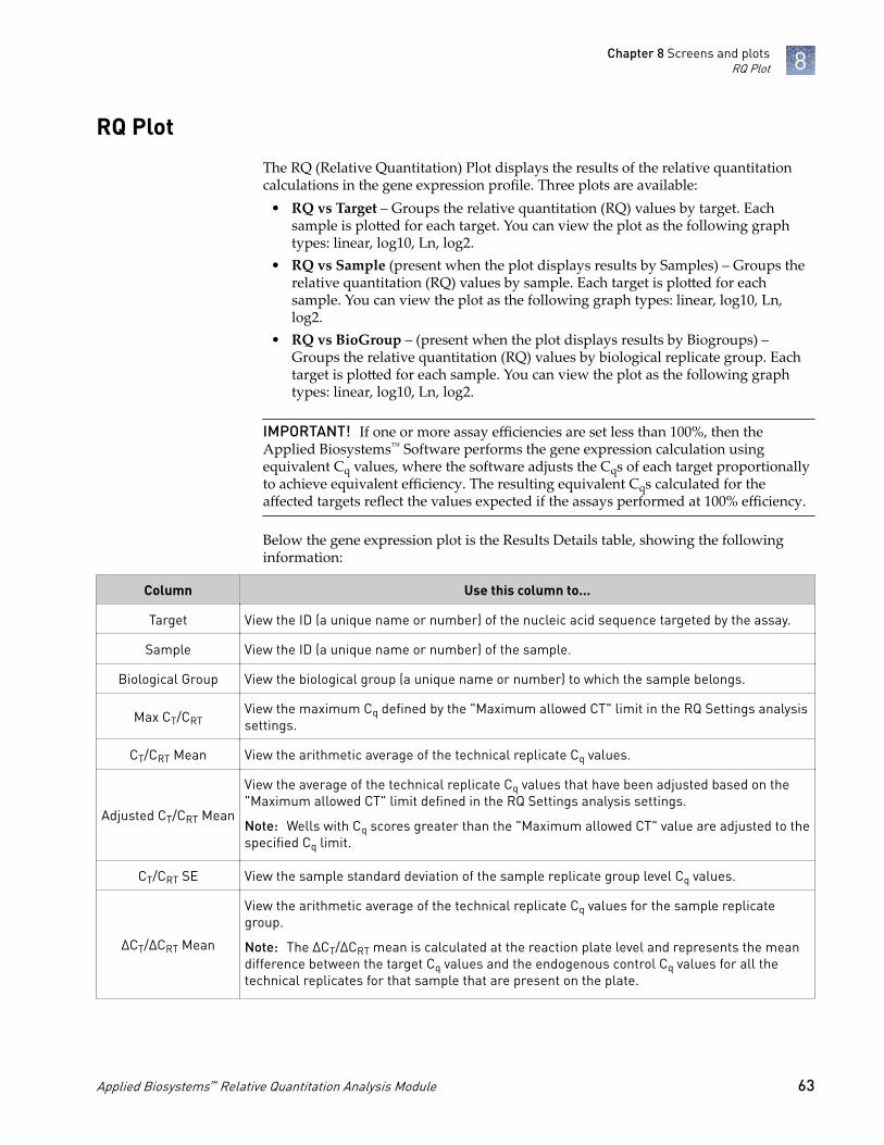
RQ Plot
The RQ (Relative Quantitation) Plot displays the results of the relative quantitationcalculations in the gene expression profile. Three plots are available:
• RQ vs Target – Groups the relative quantitation (RQ) values by target. Eachsample is plotted for each target. You can view the plot as the following graphtypes: linear, log10, Ln, log2.
• RQ vs Sample (present when the plot displays results by Samples) – Groups therelative quantitation (RQ) values by sample. Each target is plotted for eachsample. You can view the plot as the following graph types: linear, log10, Ln,log2.
• RQ vs BioGroup – (present when the plot displays results by Biogroups) –Groups the relative quantitation (RQ) values by biological replicate group. Eachtarget is plotted for each sample. You can view the plot as the following graphtypes: linear, log10, Ln, log2.
IMPORTANT! If one or more assay efficiencies are set less than 100%, then theApplied Biosystems™ Software performs the gene expression calculation usingequivalent Cq values, where the software adjusts the Cqs of each target proportionallyto achieve equivalent efficiency. The resulting equivalent Cqs calculated for theaffected targets reflect the values expected if the assays performed at 100% efficiency.
Below the gene expression plot is the Results Details table, showing the followinginformation:
Column Use this column to...
Target View the ID (a unique name or number) of the nucleic acid sequence targeted by the assay.
Sample View the ID (a unique name or number) of the sample.
Biological Group View the biological group (a unique name or number) to which the sample belongs.
Max CT/CRTView the maximum Cq defined by the "Maximum allowed CT" limit in the RQ Settings analysissettings.
CT/CRT Mean View the arithmetic average of the technical replicate Cq values.
Adjusted CT/CRT Mean
View the average of the technical replicate Cq values that have been adjusted based on the"Maximum allowed CT" limit defined in the RQ Settings analysis settings.
Note: Wells with Cq scores greater than the "Maximum allowed CT" value are adjusted to thespecified Cq limit.
CT/CRT SE View the sample standard deviation of the sample replicate group level Cq values.
∆CT/∆CRT Mean
View the arithmetic average of the technical replicate Cq values for the sample replicategroup.
Note: The ∆CT/∆CRT mean is calculated at the reaction plate level and represents the meandifference between the target Cq values and the endogenous control Cq values for all thetechnical replicates for that sample that are present on the plate.
Chapter 8 Screens and plotsRQ Plot 8
Applied Biosystems™ Relative Quantitation Analysis Module 63
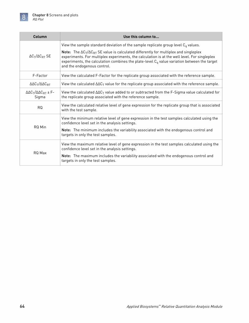
Column Use this column to...
∆CT/∆CRT SE
View the sample standard deviation of the sample replicate group level Cq values.
Note: The ∆CT/∆CRT SE value is calculated differently for multiplex and singleplexexperiments. For multiplex experiments, the calculation is at the well level. For singleplexexperiments, the calculation combines the plate-level Cq value variation between the targetand the endogenous control.
F-Factor View the calculated F-Factor for the replicate group associated with the reference sample.
∆∆CT/∆∆CRT View the calculated ΔΔCT value for the replicate group associated with the reference sample.
∆∆CT/∆∆CRT ± F-Sigma
View the calculated ΔΔCT value added to or subtracted from the F-Sigma value calculated forthe replicate group associated with the reference sample.
RQ View the calculated relative level of gene expression for the replicate group that is associatedwith the test sample.
RQ Min
View the minimum relative level of gene expression in the test samples calculated using theconfidence level set in the analysis settings.
Note: The minimum includes the variability associated with the endogenous control andtargets in only the test samples.
RQ Max
View the maximum relative level of gene expression in the test samples calculated using theconfidence level set in the analysis settings.
Note: The maximum includes the variability associated with the endogenous control andtargets in only the test samples.
Chapter 8 Screens and plotsRQ Plot8
64 Applied Biosystems™ Relative Quantitation Analysis Module
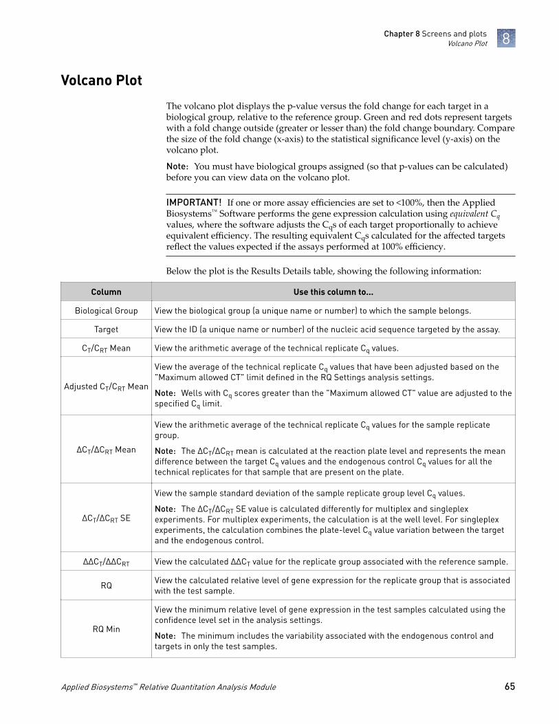
Volcano Plot
The volcano plot displays the p-value versus the fold change for each target in abiological group, relative to the reference group. Green and red dots represent targetswith a fold change outside (greater or lesser than) the fold change boundary. Comparethe size of the fold change (x-axis) to the statistical significance level (y-axis) on thevolcano plot.
Note: You must have biological groups assigned (so that p-values can be calculated)before you can view data on the volcano plot.
IMPORTANT! If one or more assay efficiencies are set to <100%, then the AppliedBiosystems™ Software performs the gene expression calculation using equivalent Cqvalues, where the software adjusts the Cqs of each target proportionally to achieveequivalent efficiency. The resulting equivalent Cqs calculated for the affected targetsreflect the values expected if the assays performed at 100% efficiency.
Below the plot is the Results Details table, showing the following information:
Column Use this column to...
Biological Group View the biological group (a unique name or number) to which the sample belongs.
Target View the ID (a unique name or number) of the nucleic acid sequence targeted by the assay.
CT/CRT Mean View the arithmetic average of the technical replicate Cq values.
Adjusted CT/CRT Mean
View the average of the technical replicate Cq values that have been adjusted based on the"Maximum allowed CT" limit defined in the RQ Settings analysis settings.
Note: Wells with Cq scores greater than the "Maximum allowed CT" value are adjusted to thespecified Cq limit.
∆CT/∆CRT Mean
View the arithmetic average of the technical replicate Cq values for the sample replicategroup.
Note: The ∆CT/∆CRT mean is calculated at the reaction plate level and represents the meandifference between the target Cq values and the endogenous control Cq values for all thetechnical replicates for that sample that are present on the plate.
∆CT/∆CRT SE
View the sample standard deviation of the sample replicate group level Cq values.
Note: The ∆CT/∆CRT SE value is calculated differently for multiplex and singleplexexperiments. For multiplex experiments, the calculation is at the well level. For singleplexexperiments, the calculation combines the plate-level Cq value variation between the targetand the endogenous control.
∆∆CT/∆∆CRT View the calculated ΔΔCT value for the replicate group associated with the reference sample.
RQ View the calculated relative level of gene expression for the replicate group that is associatedwith the test sample.
RQ Min
View the minimum relative level of gene expression in the test samples calculated using theconfidence level set in the analysis settings.
Note: The minimum includes the variability associated with the endogenous control andtargets in only the test samples.
Chapter 8 Screens and plotsVolcano Plot 8
Applied Biosystems™ Relative Quantitation Analysis Module 65
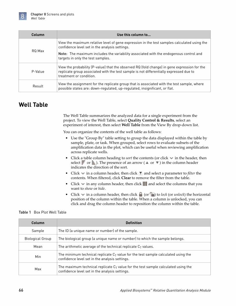
Column Use this column to...
RQ Max
View the maximum relative level of gene expression in the test samples calculated using theconfidence level set in the analysis settings.
Note: The maximum includes the variability associated with the endogenous control andtargets in only the test samples.
P-ValueView the probability (P-value) that the observed RQ (fold change) in gene expression for thereplicate group associated with the test sample is not differentially expressed due totreatment or condition.
Result View the assignment for the replicate group that is associated with the test sample, wherepossible states are: down-regulated, up-regulated, insignificant, or flat.
Well Table
The Well Table summarizes the analyzed data for a single experiment from theproject. To view the Well Table, select Quality Control & Results, select anexperiment of interest, then select Well Table from the View By drop-down list.
You can organize the contents of the well table as follows:• Use the "Group By" table setting to group the data displayed within the table by
sample, plate, or task. When grouped, select rows to evaluate subsets of theamplification data in the plot, which can be useful when reviewing amplificationacross replicate wells.
• Click a table column heading to sort the contents (or click in the header, thenselect or ). The presence of an arrow ( or ) in the column headerindicates the direction of the sort.
• Click in a column header, then click and select a parameter to filter thecontents. When filtered, click Clear to remove the filter from the table.
• Click in any column header, then click and select the columns that youwant to show or hide.
• Click in a column header, then click (or ) to lock (or unlock) the horizontalposition of the column within the table. When a column is unlocked, you canclick and drag the column header to reposition the column within the table.
Table 1 Box Plot Well Table
Column Definition
Sample The ID (a unique name or number) of the sample.
Biological Group The biological group (a unique name or number) to which the sample belongs.
Mean The arithmetic average of the technical replicate CT values.
Min The minimum technical replicate CT value for the test sample calculated using theconfidence level set in the analysis settings.
Max The maximum technical replicate CT value for the test sample calculated using theconfidence level set in the analysis settings.
Chapter 8 Screens and plotsWell Table8
66 Applied Biosystems™ Relative Quantitation Analysis Module

Column Definition
Median The median CT value for the technical replicates of the sample.
Q1
The 1st Quartile (Q1) for the sample replicate group, which is calculated as the numericmidpoint between the lowest and median CT values of the technical replicates.
Note: The 1st Quartile defines lower boundary of the inter-quartile region (IQR), which isdefined as the difference between the 3rd and 1st quartile.
Q3 The 3rd Quartile (Q3) for the sample replicate group, which is calculated as the numericmidpoint between the median and maximum CT values of the technical replicates.
Table 2 Relative Quantitation Plot Well Table
Column Definition
Target The ID (a unique name or number) of the nucleic acid sequence targeted by the assay.
Sample The ID (a unique name or number) of the sample.
Biological Group The biological group (a unique name or number) to which the sample belongs.
Max CT/CRTThe maximum Cq defined by the "Maximum allowed CT" limit in the RQ Settings analysissettings.
CT/CRT Mean The arithmetic average of the technical replicate Cq values.
Adjusted CT/CRT Mean
The average of the technical replicate Cq values that have been adjusted based on the"Maximum allowed CT" limit defined in the RQ Settings analysis settings.
Note: Wells with Cq scores greater than the "Maximum allowed CT" value are adjusted to thespecified Cq limit.
CT/CRT SE The sample standard deviation of the sample replicate group level Cq values.
∆CT/∆CRT Mean
The arithmetic average of the technical replicate Cq values for the sample replicate group.
Note: The ∆CT/∆CRT mean is calculated at the reaction plate level and represents the meandifference between the target Cq values and the endogenous control Cq values for all thetechnical replicates for that sample that are present on the plate.
∆CT/∆CRT SE
The sample standard deviation of the sample replicate group level Cq values.
Note: The ∆CT/∆CRT SE value is calculated differently for multiplex and singleplexexperiments. For multiplex experiments, the calculation is at the well level. For singleplexexperiments, the calculation combines the plate-level Cq value variation between the targetand the endogenous control.
Chapter 8 Screens and plotsWell Table 8
Applied Biosystems™ Relative Quantitation Analysis Module 67

Column Definition
F-Factor
The calculated F-Factor for the replicate group associated with the reference sample.
The F-Factor is used to calculate the RQ confidence intervals in the ∆∆CT calculation(displayed as error bars in the RQ plot). The value is calculated differently depending on theRQ Settings in the analysis settings for your project.
• If you specified a Confidence level setting, then the F-Factor is the t-value of theStudent's t-distribution calculated from the:
– Degrees of freedom that characterize the distribution of the replicate population. Ifthe project contains no biological groups, degrees of freedom is calculated perTechnical Test Sample as:#Technical Replicates WellsTarget + #Technical Replicates WellsEndo - 2.Otherwise, the value is calculated per Biological Test Sample as:#Technical Replicates Groups Test Sample - 1.
– Probability associated with the two-tailed Student's t-distribution (determined bythe RQ Settings in the analysis settings for your project).
• If you specified a Limit by standard deviations setting, then the F-Factor is equal to thesetting (1, 2, or 3).
∆∆CT/∆∆CRT The calculated ΔΔCT value for the replicate group associated with the reference sample.
∆∆CT/∆∆CRT ± F-Sigma
The calculated ΔΔCT value added to or subtracted from the F-Sigma value calculated for thereplicate group associated with the reference sample.
RQ The calculated relative level of gene expression for the replicate group that is associated withthe test sample.
RQ Min
The minimum relative level of gene expression in the test samples calculated using theconfidence level set in the analysis settings.
Note: The minimum includes the variability associated with the endogenous control andtargets in only the test samples.
RQ Max
The maximum relative level of gene expression in the test samples calculated using theconfidence level set in the analysis settings.
Note: The maximum includes the variability associated with the endogenous control andtargets in only the test samples.
Chapter 8 Screens and plotsWell Table8
68 Applied Biosystems™ Relative Quantitation Analysis Module
Quality flags
■ AMPNC (Amplification in negative control) quality flag . . . . . . . . . . . . . . . . . . . 70
■ AMPSCORE (Low signal in linear phase) quality flag . . . . . . . . . . . . . . . . . . . . . 70
■ BADROX (Bad passive reference signal) quality flag . . . . . . . . . . . . . . . . . . . . . . 71
■ BLFAIL (Baseline algorithm failed) quality flag . . . . . . . . . . . . . . . . . . . . . . . . . . . 71
■ CQCONF (Calculated confidence in the Cq value is low) quality flag . . . . . . . . 72
■ CRTAMPLITUDE (Broad Cq Amplitude) quality flag . . . . . . . . . . . . . . . . . . . . . 72
■ CRTNOISE (Cq Noise) quality flag . . . . . . . . . . . . . . . . . . . . . . . . . . . . . . . . . . . . . 72
■ CTFAIL (Cq algorithm failed) quality flag . . . . . . . . . . . . . . . . . . . . . . . . . . . . . . . 72
■ DRNMIN (Detection of minimum DRn due to abnormal baseline)quality flag . . . . . . . . . . . . . . . . . . . . . . . . . . . . . . . . . . . . . . . . . . . . . . . . . . . . . . . . . . 73
■ EXPFAIL (Exponential algorithm failed) quality flag . . . . . . . . . . . . . . . . . . . . . . 73
■ HIGHSD (High standard deviation in replicate group) quality flag . . . . . . . . . . 74
■ LOWROX (Low ROX™ Intensity) quality flag . . . . . . . . . . . . . . . . . . . . . . . . . . . . 75
■ MAXCT (Cq above maximum) quality flag . . . . . . . . . . . . . . . . . . . . . . . . . . . . . . 75
■ MPOUTLIER (ΔCq outlier in multiplex experiment) quality flag . . . . . . . . . . . . 75
■ MTP (Melt curve analysis shows more than one peak) quality flag . . . . . . . . . . 75
■ NOAMP (No amplification) quality flag . . . . . . . . . . . . . . . . . . . . . . . . . . . . . . . . . 76
■ NOISE (Noise higher than others in plate) quality flag . . . . . . . . . . . . . . . . . . . . 76
■ NOSAMPLE (No sample assigned to well) quality flag . . . . . . . . . . . . . . . . . . . . 77
■ NOSIGNAL (No signal in well) quality flag . . . . . . . . . . . . . . . . . . . . . . . . . . . . . . 77
■ OFFSCALE (Fluorescence is offscale) quality flag . . . . . . . . . . . . . . . . . . . . . . . . . 78
■ OUTLIERRG (Outlier in replicate group) quality flag . . . . . . . . . . . . . . . . . . . . . 79
■ PRFDROP (Passive reference signal changes significantly near theCq/Ct) quality flag . . . . . . . . . . . . . . . . . . . . . . . . . . . . . . . . . . . . . . . . . . . . . . . . . . . . 79
■ PRFLOW (Average passive reference signal is below the threshold)quality flag . . . . . . . . . . . . . . . . . . . . . . . . . . . . . . . . . . . . . . . . . . . . . . . . . . . . . . . . . . 80
■ SPIKE (Noise spikes) quality flag . . . . . . . . . . . . . . . . . . . . . . . . . . . . . . . . . . . . . . . 81
■ THOLDFAIL (Thresholding algorithm failed) quality flag . . . . . . . . . . . . . . . . . 81
9
Applied Biosystems™ Relative Quantitation Analysis Module 69
AMPNC (Amplification in negative control) quality flag
The AMPNC ( ) quality flag indicates that a sequence in a negative control reactionamplified.
If a well is flagged, confirm the results:
1. Select the flagged well(s) in the plate layout or well table.2. Make sure that the well corresponds to a negative control well (Task = Negative
Control or NTC).3. View the amplification plot [∆Rn vs. Cycle (Linear) or ∆Rn vs. Cycle (Log)], andconfirm the fluorescence signal increased for the flagged negative control well. Ifthe fluorescence signal did not increase, omit the well from analysis.
Possible Cause Recommended Action
Contamination in one ormore PCR reactioncomponents
• Replace all PCR reaction components with newcomponents, then repeat the experiment. Make sureto add water or buffer instead of sample to the well.
• Decontaminate the work area and pipettors.
Unstable reaction mix • Use a hot-start enzyme.
• If you are not using a hot-start enzyme, run thereactions as soon as possible after you prepare them.
Poor primer and/or probedesign
Redesign the primers and/or probe.
AMPSCORE (Low signal in linear phase) quality flag
The AMPSCORE ( ) quality flag indicates that, for a given well, the amplification inthe linear region is below a certain threshold, corresponding to the score set in theanalysis settings.
Use the AMPSCORE flag to easily identify and, optionally, omit potentially poorresults without manually inspecting every amplification curve. The numeric value forthe amplification score is found in the Amp Score column of the well table for theamplification and multicomponent plots.
Note: For Quantitative or Genotyping applications, this flag is only appropriate whenROX™ dye is used as the passive reference or the data is from OpenArray™ plates. ForAbsolute Quantification applications, this flag is only appropriate when ROX™ dye isused as the passive reference.
If a well is flagged, confirm the results:
1. Select the flagged well(s) in the plate layout or well table.2. Make sure that the well does not correspond to a negative-control (NTC) well.3. View the amplification plot [DRn vs. Cycle (Linear) or DRn vs. Cycle (Log)], and
check the shape of the curve. If the curve is atypical, consider omitting theflagged well(s) from analysis.
Chapter 9 Quality flagsAMPNC (Amplification in negative control) quality flag9
70 Applied Biosystems™ Relative Quantitation Analysis Module

BADROX (Bad passive reference signal) quality flag
The BADROX ( ) quality flag indicates that the passive reference (usually ROX™
dye) signal is abnormal. The passive reference signal may not be acceptable fornormalization of the reporter dye signal.
If a well is flagged, confirm the results:
1. Select the flagged well(s) in the plate layout or well table.2. View the multicomponent plot, and review the passive reference signal for
abnormalities.3. View the amplification plot [DRn vs. Cycle (Linear) or DRn vs. Cycle (Log)], and
review the data in the Cq region for abnormalities.4. Examine the reaction plate, and check for condensation and/or inconsistent
reaction volumes.
Possible Cause Recommended Action
Droplets on the sides of thewells.
Repeat the experiment, and make sure you centrifuge theplate briefly before loading it into the instrument.
Evaporation resulting fromimproper sealing or sealleaks. Repeat the reactions, and make sure you seal the plate
properly.Condensation on thereaction plate.
Inconsistent volumes acrossthe plate.
Confirm that pipettes are calibrated and functioningproperly.
Incorrect concentration ofreference dye.
Confirm that you are using the appropriate master mix foryour instrument.
Pipetting errors. Calibrate your pipettors, then repeat the experiment.
BLFAIL (Baseline algorithm failed) quality flag
Note: The BLFAIL flag is only valid when you use the Baseline Threshold algorithmto analyze your experiments, though it is always shown in the QC Summary.
The BLFAIL ( ) quality flag indicates that the automatic baseline algorithm failed,and the software cannot calculate the best-fit baseline for the data.
If a well is flagged, confirm the results:
1. Select the flagged well(s) in the plate layout or well table.2. View the amplification plot [DRn vs. Cycle (Linear) or DRn vs. Cycle (Log)], and
check for late amplification or no amplification.3. If the amplification looks acceptable, set the baseline manually.4. Click Analyze to reanalyze the data.5. Evaluate the results and, if needed, make any additional changes to the baseline.
Chapter 9 Quality flagsBADROX (Bad passive reference signal) quality flag 9
Applied Biosystems™ Relative Quantitation Analysis Module 71
CQCONF (Calculated confidence in the Cq value is low) quality flag
The CQCONF ( ) quality flag indicates that the calculated confidence for the Cq/CTvalue of the well is less than the minimum value defined in the analysis settings.
Use the CQCONF flag to easily identify and, optionally, omit potentially poor resultswithout manually inspecting every amplification curve. The minimum limit is set inthe Flag Settings tab of the Analysis Settings dialog box.
If a well is flagged, confirm the results:
1. Select the flagged well(s) in the plate layout or well table.2. View the amplification plot [DRn vs. Cycle (Linear) or DRn vs. Cycle (Log)], and
check the shape of the curve. If the curve is atypical, consider omitting theflagged well(s) from analysis.
CRTAMPLITUDE (Broad Cq Amplitude) quality flag
The CRTAMPLITUDE ( ) quality flag indicates that the amplitude of the relativestandard curve, generated from the data set that includes the given well, issignificantly lower than the other curves generated for the related target.
CRTNOISE (Cq Noise) quality flag
The CRTNOISE quality flag indicates that for the relative standard curve, generatedfrom the data set that includes the given well, exhibited a significant amount ofunexplained variability in comparison to the other curves generated for the relatedtarget.
CTFAIL (Cq algorithm failed) quality flag
Note: The CTFAIL flag is only valid when you use the Baseline Threshold algorithmto analyze your experiments, though it is always shown in the QC Summary.
The CTFAIL ( ) quality flag indicates that the automatic Cq algorithm failed for thegiven well, and the software cannot calculate the threshold cycle (Cq).
If a well is flagged, confirm the results:
1. Select the flagged well(s) in the plate layout or well table.2. View the amplification plot [DRn vs. Cycle (Linear) or DRn vs. Cycle (Log)] and
check for:• Amplification too early• Amplification too late• Low amplification• No amplification
3. If the amplification looks acceptable, set the threshold and baseline manually.
Chapter 9 Quality flagsCQCONF (Calculated confidence in the Cq value is low) quality flag9
72 Applied Biosystems™ Relative Quantitation Analysis Module
4. Click Analyze to reanalyze the data.5. Evaluate the results. If the adjustments do not produce a valid Cq, consideromitting the well from analysis.
DRNMIN (Detection of minimum DRn due to abnormal baseline)quality flag
The DRNMIN ( ) quality flag indicates that the normalized fluorescence (DRn) for agiven well dropped below the threshold defined in the analysis settings.
Use the DRNMIN flag to easily identify and, optionally, omit potentially poor resultswithout manually inspecting every amplification curve. The DRn threshold value isset in the Flag Settings tab of the Analysis Settings dialog box.
If a well is flagged, confirm the results:
1. Select the flagged well(s) in the plate layout or well table.2. View the amplification and multicomponent plots [DRn vs. Cycle (Linear) or DRn
vs. Cycle (Log)], and check the shape of the curve. If the curve is atypical,consider omitting the flagged well(s) from analysis.
EXPFAIL (Exponential algorithm failed) quality flag
Note: The EXPFAIL flag is only valid when you use the Baseline Threshold algorithmto analyze your experiments, though it is always shown in the QC Summary.
The EXPFAIL ( ) quality flag indicates that the automatic Cq algorithm failed for thegiven well, and the software cannot identify the exponential region of theamplification plot.
If a well is flagged, confirm the results:
1. Select the flagged well(s) in the plate layout or well table.2. View the amplification plot [ DRn vs. Cycle (Linear) or DRn vs. Cycle (Log)], and
check for:• Amplification too early• Amplification too late• Low amplification• No amplification
3. If the amplification looks acceptable, set the threshold manually:
a. Click the threshold (the horizontal line across the plot) and drag it up ordown to a location within the exponential region of the amplification.
b. Click Analyze to reanalyze the data.c. Evaluate the results and, if needed, make any additional changes to the
threshold.
Chapter 9 Quality flagsDRNMIN (Detection of minimum DRn due to abnormal baseline) quality flag 9
Applied Biosystems™ Relative Quantitation Analysis Module 73
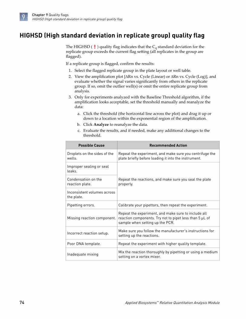
HIGHSD (High standard deviation in replicate group) quality flag
The HIGHSD ( ) quality flag indicates that the Cq standard deviation for thereplicate group exceeds the current flag setting (all replicates in the group areflagged).
If a replicate group is flagged, confirm the results:
1. Select the flagged replicate group in the plate layout or well table.2. View the amplification plot [DRn vs. Cycle (Linear) or DRn vs. Cycle (Log)], and
evaluate whether the signal varies significantly from others in the replicategroup. If so, omit the outlier well(s) or omit the entire replicate group fromanalysis.
3. Only for experiments analyzed with the Baseline Threshold algorithm, if theamplification looks acceptable, set the threshold manually and reanalyze thedata:
a. Click the threshold (the horizontal line across the plot) and drag it up ordown to a location within the exponential region of the amplification.
b. Click Analyze to reanalyze the data.c. Evaluate the results, and if needed, make any additional changes to the
threshold.
Possible Cause Recommended Action
Droplets on the sides of thewells.
Repeat the experiment, and make sure you centrifuge theplate briefly before loading it into the instrument.
Improper sealing or sealleaks.
Repeat the reactions, and make sure you seal the plateproperly.
Condensation on thereaction plate.
Inconsistent volumes acrossthe plate.
Pipetting errors. Calibrate your pipettors, then repeat the experiment.
Missing reaction component.Repeat the experiment, and make sure to include allreaction components. Try not to pipet less than 5 µL ofsample when setting up the PCR.
Incorrect reaction setup. Make sure you follow the manufacturer's instructions forsetting up the reactions.
Poor DNA template. Repeat the experiment with higher quality template.
Inadequate mixing Mix the reaction thoroughly by pipetting or using a mediumsetting on a vortex mixer.
Chapter 9 Quality flagsHIGHSD (High standard deviation in replicate group) quality flag9
74 Applied Biosystems™ Relative Quantitation Analysis Module

LOWROX (Low ROX™ Intensity) quality flag
A Low ROX™ Intensity ( ) quality flag can be raised for any data point. If the ROX™
dye intensity determined by the software for a data point is below the threshold, aflag will be raised.
If a well is flagged, no action should be taken for the data point. If the ROX™ dyeintensity is below the default threshold, the data point does not meet the minimumconditions for assigning a call.
MAXCT (Cq above maximum) quality flag
The MAXCT ( ) quality flag indicates that the mean Cq for the replicate group isabove the maximum allowed value.
The maximum allowed value is set in the Flag Settings tab of the Analysis Settingsdialog box. If the mean Cq of the replicate group is above the maximum, the softwareadjusts it to the maximum allowed value (shown in the Adjusted Cq column in thewell table).
MPOUTLIER (ΔCq outlier in multiplex experiment) quality flag
The MPOUTLIER quality flag indicates that the ΔCT for the targets in the well is lessthan the current flag setting.
If a replicate group is flagged, confirm the results:
1. Select the flagged well(s) in the plate layout or well table.2. View the amplification plot [ΔRn vs. Cycle (Linear) or ΔRn vs. Cycle (Log)] for
both targets in the well, and make sure that they both amplified.3. Only for experiments analyzed with the Baseline Threshold algorithm, set the
baseline and threshold values manually.4. Click Analyze to reanalyze the project.5. Evaluate the results. If the adjustments do not produce a valid Cq, consideromitting the well from analysis.
MTP (Melt curve analysis shows more than one peak) quality flag
The MTP ( ) quality flag indicates that the melt curve generated from the collecteddata exhibits multiple peaks, indicating possible PCR irregularities such ascontamination or nonspecific amplification.
Note: The MTP flag is present only in experiments with PCR methods that include amelting curve stage (a temperature ramp configured for data collection).
If a replicate group is flagged, confirm the results in the Melt Curve Plot. Peaks in themelt curve can indicate the melting temperature (Tm) of a target nucleic acid ornonspecific PCR amplification.
Chapter 9 Quality flagsLOWROX (Low ROX™ Intensity) quality flag 9
Applied Biosystems™ Relative Quantitation Analysis Module 75

NOAMP (No amplification) quality flag
The NOAMP ( ) quality flag indicates that the sample did not amplify.
If a well is flagged, confirm the results:
1. Select the flagged well(s) in the plate layout or well table.2. Make sure that the well does not correspond to a negative-control well.3. View the amplification plot [DRn vs. Cycle (Linear) or DRn vs. Cycle (Log)], and
make sure that the fluorescence signal did not increase in the well.4. View the multicomponent plot, and look for fluorescence signal higher than the
background.
Possible Cause Recommended Action
Missing template. Repeat the experiment, and make sure to include allreaction components.
Target is not expressed inthe sample.
• If this occurs in just one sample, it may be correct.
• If this occurs in all samples of a particular tissue,search the literature for evidence that the target isexpressed in the tissue or sample type of interest.
NOISE (Noise higher than others in plate) quality flag
The NOISE ( ) quality flag indicates that the well produced more noise in theamplification plot than the other wells on the same plate.
If a well is flagged, confirm the results:
1. Select the flagged well(s) and some unflagged unknown wells in the plate layoutor well table.
2. View the amplification plot [DRn vs. Cycle (Linear) or DRn vs. Cycle (Log)] andcheck for a noisy amplification curve in the flagged wells.
3. In the multicomponent plot:
a. From the Color by drop-down list, select Dye to color the data according tothe dye.
b. Check for a drop in ROX™ signal relative to the reporter dye and compareflagged wells with unflagged wells.
c. If there is a drop in the ROX™ signal compared to the reporter dye, consideromitting the flagged well(s) from analysis.
Chapter 9 Quality flagsNOAMP (No amplification) quality flag9
76 Applied Biosystems™ Relative Quantitation Analysis Module
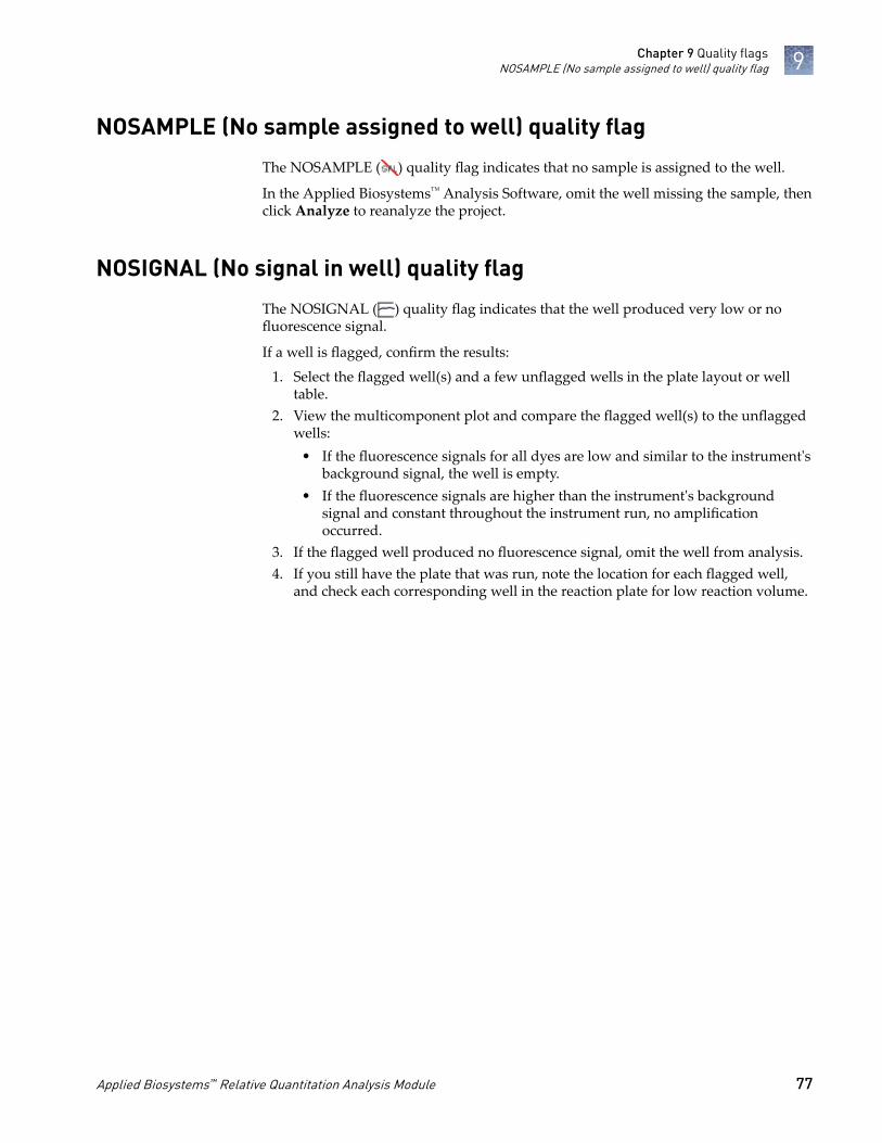
NOSAMPLE (No sample assigned to well) quality flag
The NOSAMPLE ( ) quality flag indicates that no sample is assigned to the well.
In the Applied Biosystems™ Analysis Software, omit the well missing the sample, thenclick Analyze to reanalyze the project.
NOSIGNAL (No signal in well) quality flag
The NOSIGNAL ( ) quality flag indicates that the well produced very low or nofluorescence signal.
If a well is flagged, confirm the results:
1. Select the flagged well(s) and a few unflagged wells in the plate layout or welltable.
2. View the multicomponent plot and compare the flagged well(s) to the unflaggedwells:
• If the fluorescence signals for all dyes are low and similar to the instrument'sbackground signal, the well is empty.
• If the fluorescence signals are higher than the instrument's backgroundsignal and constant throughout the instrument run, no amplificationoccurred.
3. If the flagged well produced no fluorescence signal, omit the well from analysis.4. If you still have the plate that was run, note the location for each flagged well,
and check each corresponding well in the reaction plate for low reaction volume.
Chapter 9 Quality flagsNOSAMPLE (No sample assigned to well) quality flag 9
Applied Biosystems™ Relative Quantitation Analysis Module 77

OFFSCALE (Fluorescence is offscale) quality flag
The OFFSCALE ( ) quality flag indicates that the fluorescence signal for one or moredyes in the well exceeds the instrument's maximum detectable range for one or morecycles.
Confirm the results:
1. Select the flagged well(s) in the plate layout or well table.2. View the amplification plot [DRn vs. Cycle (Linear) or DRn vs. Cycle (Log)] or the
well table, and note the threshold cycle.3. View the multicomponent plot, and review the data for a plateau over one or
more cycles. A plateau indicates saturation of the instrument's detectors. If thesignal plateaus before the threshold cycle, omit the well(s).
Possible Cause Recommended Action
Too much TaqMan® probe orSYBR™ Green dye added tothe reaction.
Reduce the concentration of reagent added to the reaction.
Fluorescent contaminant onthe reaction plate, sampleblock, or adhesive cover.
Perform a background calibration. If you detect fluorescentcontamination, clean the block.
Fluorescent contaminant inthe reaction.
Replace the reagents.
Chapter 9 Quality flagsOFFSCALE (Fluorescence is offscale) quality flag9
78 Applied Biosystems™ Relative Quantitation Analysis Module
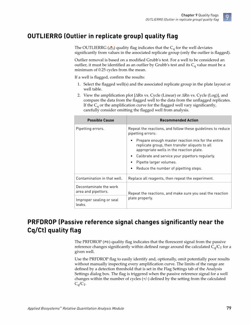
OUTLIERRG (Outlier in replicate group) quality flag
The OUTLIERRG ( ) quality flag indicates that the Cq for the well deviatessignificantly from values in the associated replicate group (only the outlier is flagged).
Outlier removal is based on a modified Grubb's test. For a well to be considered anoutlier, it must be identified as an outlier by Grubb's test and its Cq value must be aminimum of 0.25 cycles from the mean.
If a well is flagged, confirm the results:
1. Select the flagged well(s) and the associated replicate group in the plate layout orwell table.
2. View the amplification plot [∆Rn vs. Cycle (Linear) or ∆Rn vs. Cycle (Log)], andcompare the data from the flagged well to the data from the unflagged replicates.If the Cq or the amplification curve for the flagged well vary significantly,carefully consider omitting the flagged well from analysis.
Possible Cause Recommended Action
Pipetting errors. Repeat the reactions, and follow these guidelines to reducepipetting errors:
• Prepare enough master reaction mix for the entirereplicate group, then transfer aliquots to allappropriate wells in the reaction plate.
• Calibrate and service your pipettors regularly.
• Pipette larger volumes.
• Reduce the number of pipetting steps.
Contamination in that well. Replace all reagents, then repeat the experiment.
Decontaminate the workarea and pipettors. Repeat the reactions, and make sure you seal the reaction
plate properly.Improper sealing or sealleaks.
PRFDROP (Passive reference signal changes significantly near theCq/Ct) quality flag
The PRFDROP ( ) quality flag indicates that the florescent signal from the passivereference changes significantly within defined range around the calculated Cq/CT for agiven well.
Use the PRFDROP flag to easily identify and, optionally, omit potentially poor resultswithout manually inspecting every amplification curve. The limits of the range aredefined by a detection threshold that is set in the Flag Settings tab of the AnalysisSettings dialog box. The flag is triggered when the passive reference signal for a wellchanges within the number of cycles (+/-) defined by the setting from the calculatedCq/CT.
Chapter 9 Quality flagsOUTLIERRG (Outlier in replicate group) quality flag 9
Applied Biosystems™ Relative Quantitation Analysis Module 79
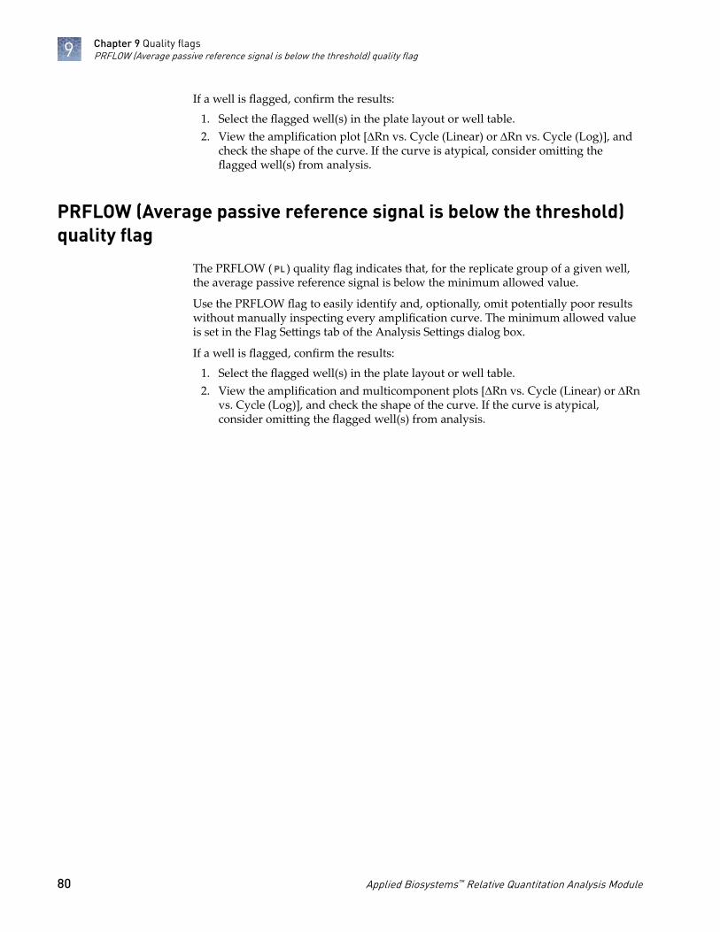
If a well is flagged, confirm the results:
1. Select the flagged well(s) in the plate layout or well table.2. View the amplification plot [DRn vs. Cycle (Linear) or DRn vs. Cycle (Log)], and
check the shape of the curve. If the curve is atypical, consider omitting theflagged well(s) from analysis.
PRFLOW (Average passive reference signal is below the threshold)quality flag
The PRFLOW ( ) quality flag indicates that, for the replicate group of a given well,the average passive reference signal is below the minimum allowed value.
Use the PRFLOW flag to easily identify and, optionally, omit potentially poor resultswithout manually inspecting every amplification curve. The minimum allowed valueis set in the Flag Settings tab of the Analysis Settings dialog box.
If a well is flagged, confirm the results:
1. Select the flagged well(s) in the plate layout or well table.2. View the amplification and multicomponent plots [DRn vs. Cycle (Linear) or DRn
vs. Cycle (Log)], and check the shape of the curve. If the curve is atypical,consider omitting the flagged well(s) from analysis.
Chapter 9 Quality flagsPRFLOW (Average passive reference signal is below the threshold) quality flag9
80 Applied Biosystems™ Relative Quantitation Analysis Module
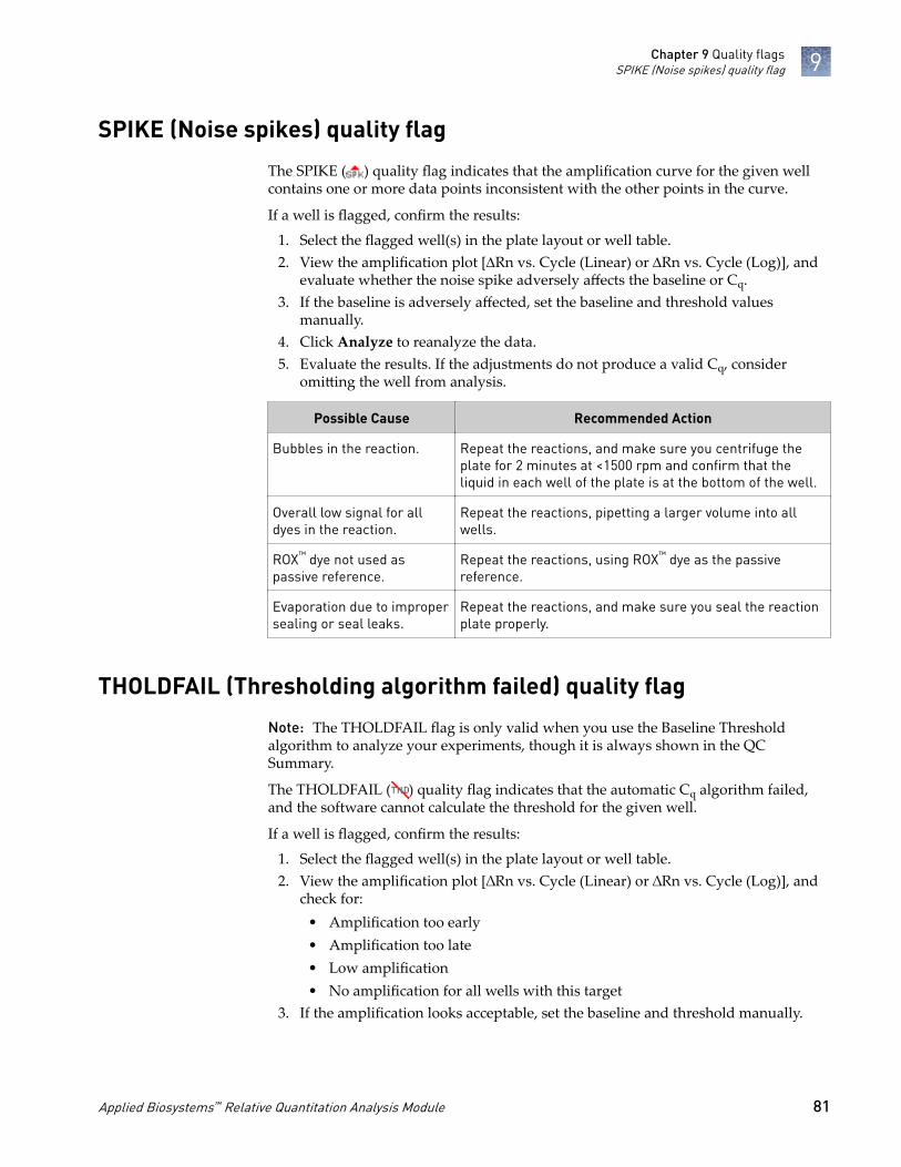
SPIKE (Noise spikes) quality flag
The SPIKE ( ) quality flag indicates that the amplification curve for the given wellcontains one or more data points inconsistent with the other points in the curve.
If a well is flagged, confirm the results:
1. Select the flagged well(s) in the plate layout or well table.2. View the amplification plot [DRn vs. Cycle (Linear) or DRn vs. Cycle (Log)], and
evaluate whether the noise spike adversely affects the baseline or Cq.3. If the baseline is adversely affected, set the baseline and threshold values
manually.4. Click Analyze to reanalyze the data.5. Evaluate the results. If the adjustments do not produce a valid Cq, consideromitting the well from analysis.
Possible Cause Recommended Action
Bubbles in the reaction. Repeat the reactions, and make sure you centrifuge theplate for 2 minutes at <1500 rpm and confirm that theliquid in each well of the plate is at the bottom of the well.
Overall low signal for alldyes in the reaction.
Repeat the reactions, pipetting a larger volume into allwells.
ROX™ dye not used aspassive reference.
Repeat the reactions, using ROX™ dye as the passivereference.
Evaporation due to impropersealing or seal leaks.
Repeat the reactions, and make sure you seal the reactionplate properly.
THOLDFAIL (Thresholding algorithm failed) quality flag
Note: The THOLDFAIL flag is only valid when you use the Baseline Thresholdalgorithm to analyze your experiments, though it is always shown in the QCSummary.
The THOLDFAIL ( ) quality flag indicates that the automatic Cq algorithm failed,and the software cannot calculate the threshold for the given well.
If a well is flagged, confirm the results:
1. Select the flagged well(s) in the plate layout or well table.2. View the amplification plot [∆Rn vs. Cycle (Linear) or ∆Rn vs. Cycle (Log)], and
check for:• Amplification too early• Amplification too late• Low amplification• No amplification for all wells with this target
3. If the amplification looks acceptable, set the baseline and threshold manually.
Chapter 9 Quality flagsSPIKE (Noise spikes) quality flag 9
Applied Biosystems™ Relative Quantitation Analysis Module 81
4. Click Analyze to reanalyze the data.5. Evaluate the results and, if needed, make any additional changes to the threshold
or baseline.
Chapter 9 Quality flagsTHOLDFAIL (Thresholding algorithm failed) quality flag9
82 Applied Biosystems™ Relative Quantitation Analysis Module

Documentation and support
■ Customer and technical support . . . . . . . . . . . . . . . . . . . . . . . . . . . . . . . . . . . . . . . . 83
■ Limited product warranty . . . . . . . . . . . . . . . . . . . . . . . . . . . . . . . . . . . . . . . . . . . . . 83
Customer and technical support
Visit thermofisher.com/support for the latest in services and support, including:• Worldwide contact telephone numbers• Product support, including:
– Product FAQs– Software, patches, and updates
• Order and web support• Product documentation, including:
– User guides, manuals, and protocols– Certificates of Analysis– Safety Data Sheets (SDSs; also known as MSDSs)
Note: For SDSs for reagents and chemicals from other manufacturers,contact the manufacturer.
Limited product warranty
Life Technologies Corporation and/or its affiliate(s) warrant their products as set forthin the Life Technologies' General Terms and Conditions of Sale found on LifeTechnologies' website at www.thermofisher.com/us/en/home/global/terms-and-conditions.html. If you have any questions, please contact LifeTechnologies at www.thermofisher.com/support.
A
Applied Biosystems™ Relative Quantitation Analysis Module 83

Glossary
Assay information files are delivered on Information CDs that accompany TaqMan®
assay orders. Each assay information file contains reference information about theassociated order and technical details of all assays in the shipment.
You can import an assay information file into the Applied Biosystems™ AnalysisSoftware to add supplementary assay information to a project. Assay information filesare available in three formats (.html, .txt, and .xml), but the Applied Biosystems™
Analysis Software supports only .txt and .xml files.
IMPORTANT! The assay information file must include an assay ID (in the Assay IDcolumn) for each assay listed in the file. The software matches the assay IDs in theassay information file with the existing assay IDs in the project.
IMPORTANT! When you import an assay information file, information from the filepopulates the corresponding columns in the Assays list in the Overview screen. Alldata in the Overview screen are replaced for all assays that are identified in the assayinformation file. If the assay information file does not contain information for anassay, the existing data in the Overview screen is unaffected.
Calculation of the efficiency of the PCR amplification in a standard curve experiment.EFF% is calculated using the slope of the regression line in the standard curve. Aslope close to -3.32 indicates optimal, 100% PCR amplification efficiency. To useamplification efficiency in a gene expression project:
• On the instrument where you collected the comparative CT (∆∆CT) data that willbe used in the project, run a standard curve experiment to determine theefficiency.
• In the Applied Biosystems™ Analysis Software, enter the amplification efficiencyin the Efficiency table in the Relative Quantification Settings tab in the AnalysisSettings dialog box.
Display of data collected during the cycling stage of PCR amplification. Theamplification plot can be viewed as:
• Baseline-corrected normalized reporter (∆Rn) vs. cycle• Normalized reporter (Rn) vs. cycle
An analysis group is a project setting that allows you to create a profile of the analysisand quality settings for the analysis of a project. Analysis groups can be applied eitherglobally to analyze an entire project, or exclusively to a subset of the experiments orsamples added to a project. Later in the analysis, the Applied Biosystems™ AnalysisSoftware allows you to switch between analysis groups so that you can compare theeffects of changes to the analysis settings on your results.
assay informationfiles
amplificationefficiency (EFF%)
amplification plot
analysis group
84 Applied Biosystems™ Relative Quantitation Analysis Module
A PCR reaction mix that contains primers to amplify a target and a reagent to detectthe amplified target.
An analysis setting for the Baseline Threshold algorithm in which the softwareidentifies the start and end cycles for the baseline in the amplification plot.
An analysis setting for the Baseline Threshold algorithm in which the softwarecalculates the baseline start and end cycles and the threshold in the amplification plot.The software uses the baseline and threshold to calculate the threshold cycle (Cq).
In the amplification plot, the baseline is a cycle-to-cycle range that defines backgroundfluorescence. This range can be set manually on a target-by-target basis, orautomatically, where the software sets the baseline for each individual well.
Expression estimation algorithm (Cq) which subtracts a baseline component and sets afluorescent threshold in the exponential region for quantification.
In experiments that contain data from real-time PCR, the magnitude of normalizedfluorescence signal generated by the reporter at each cycle during the PCRamplification. In the ∆Rn vs Cycle amplification plot, ∆Rn is calculated at each cycleas:
∆Rn (cycle) = Rn (cycle) - Rn (baseline), where Rn = normalized reporter
Reactions that contain identical components and volumes, but evaluate separatesamples of the same biological source (for example, samples from three different miceof the same strain, or separate extractions of the same cell line or tissue sample).
When an experiment uses biological replicate groups in a gene expression project, thevalues displayed in the Biological Replicates tab are calculated by combining theresults of the separate biological samples and treating this collection as a singlepopulation (that is, as one sample). For Cq computations (normalizing by theendogenous control) in a singleplex experiment, the software averages technicalreplicates. The averages from the technical replicates are then averaged together todetermine the value for that biological replicate.
Display of the distribution of Cq values in each sample or for each target. For each boxin the plot:
• The solid box shows the range of the middle 50% of the Cq values for the target orthe sample.
• The horizontal black bar shows the median Cq value.• The black circle shows the mean Cq value.• The ends of the vertical lines (or "whiskers") show the maximum and minimum
Cq values, unless outliers are present.
assays
automaticbaseline
automaticthreshold
baseline
BaselineThresholdalgorithm
baseline-correctednormalizedreporter (∆Rn)
biologicalreplicates
box plot
Limited product warranty
Applied Biosystems™ Relative Quantitation Analysis Module 85
• Mild outliers are displayed as open circles and represent samples or targets withCq values up to 1.5X the inter-quartile region (IQR). The IQR is the differencebetween the 3rd quartile and the 1st quartile. There is one circle for each Cq inthis range.
• Extreme outliers are displayed as open triangles and represent samples or targetswith Cq values up to 3.0X the IQR. There is one triangle for each Cq in this range.
Method for determining relative target quantity ("RQ" or fold change) in samples. Thesoftware measures amplification of the target and of the endogenous control insamples and in a reference sample. Measurements are normalized using theendogenous control or global normalization. The software determines the RQ (foldchange) of target in each sample by comparing normalized target quantity in eachsample to normalized target quantity in the reference sample.
A measure of the strength of the linear relationship between two variables. Thesoftware calculates the correlation coefficient (r) for either Cq or ∆Cq for all targets in apair of samples or a pair of biological groups, for all samples and biological groups inthe study. r can range from -1 to 1.
• If r is close to 0, there is no relationship between the Cq values for the twosamples or groups.
• If r is positive, as the Cq value for one sample (or groups) increases, so does theother.
• If r is negative, as the Cq value for one sample (or group) increases, the otherdecreases (often called an "inverse" correlation).
See relative threshold cycle (CRT).
See Relative Threshold algorithm.
See threshold cycle (CT).
See threshold cycle (CT).
See threshold cycle (CT).
See Baseline Threshold algorithm.
See baseline-corrected normalized reporter (∆Rn).
See amplification efficiency (EFF%).
A feature in the software that mathematically compensates for differences inamplification efficiency of the targets and endogenous controls when calculatingrelative quantities. The software requires you to enter amplification efficiencies toperform the correction.
comparative CT(∆∆CT) method
correlationcoefficient
CRT
CRT algorithm
cycle threshold
cycling stage
CT
CT algorithm
delta Rn (∆Rn)
EFF%
efficiencycorrection
Limited product warranty
86 Applied Biosystems™ Relative Quantitation Analysis Module

To use efficiency correction in a gene expression project:
• On the instrument where you collected the comparative CT (∆∆CT) data that willbe used in the project, run a standard curve experiment to determine theefficiency.
• In Applied Biosystems™ Analysis Software, enter the amplification efficiency inthe Efficiency table in the Relative Quantification Settings tab in the AnalysisSettings dialog box.
A gene (or genes) used to correct for different amounts of starting material of RNA.Many genes can be candidates for endogenous controls, but the consistency ofexpression in different samples and different treatments should be validatedexperimentally.
Global normalization is an alternate normalization method.
For more information about selecting an endogenous control, see the application noteUsing TaqMan® Endogenous Control Assays to Select an Endogenous Control forExperimental Studies (Pub. no. CO16806) available from the Thermo Fisher Scientificweb site.
A quality control (QC) indicator which, when applied by the software to a well duringanalysis, indicates a possible issue with that reaction. A summary of the flagsidentified in the project is displayed in the Flag Summary screen.
Display of RQ versus sample or RQ versus target. RQ for the targets in the referencesample or group is always 0. The error bars indicate RQ minimum and maximum.
The mean Cq of the endogenous controls for the project. If you are using globalnormalization, the global control mean is the median of all values used for globalnormalization.
A method to correct for different amounts of starting material of RNA. Globalnormalization first finds the assays common to every sample and then uses themedian Cq of those assays as the normalization factor, on a per sample basis. It hasbeen shown that this type of normalization is only valid if a large number (384 orgreater) of genes are profiled. As an alternative to global normalization, one or moretargets can be selected as the endogenous control.
Global normalization is described in Mestdagh P.,Van Vlierberghe P., De Weer A., et al.2009. A novel and universal method for microRNA RT-qPCR data normalization.Genome Biology 10, R64.
A representation of the level of expression of many targets (genes) across a number ofcomparable samples. The targets and samples are clustered according to the similarityof their gene expression, using unsupervised hierarchical clustering. The colorindicates a change from the mean ΔCT (ΔCRT) value. Red or yellow is an increase,green or blue is a decrease.
endogenouscontrol
flag
gene expressionplot
global controlmean
globalnormalization
heat map
Limited product warranty
Applied Biosystems™ Relative Quantitation Analysis Module 87

The "zero" point for the color scale (representing no change in expression) is setdifferently for each plot type:
• Global (ΔCT) - The mean ΔCT for all targets in the project.• Global (ΔCT Plus) - For studies using an endogenous control, the median of all
(ΔCT + the global control mean) values for all targets in the project. For studiesusing global normalization, the median of all (ΔCT + the global control median)values for all targets in the project.
• Target-centric - The median of all ΔCT values for all samples for that target (datapoints for a given target can only be compared relative to other data points forthat target).
• Sample-centric - For each sample, the middle expression is set as the mean ΔCTfor all targets in the sample.
An analysis setting for the Baseline Threshold algorithm in which you enter thebaseline start and end cycles for the amplification plot for a target. If you edit thebaseline start and end cycles, the settings are applied to all instances of that target inthe project.
An analysis setting for the Baseline Threshold algorithm in which you enter thethreshold value and select whether to use automatic baseline or manual baselinevalues. The software uses the baseline and threshold values to calculate the thresholdcycle (Cq).
A plot of the complete spectral contribution of each dye for the selected well(s) overthe duration of the PCR run.
See no template control (NTC).
In the software, the task for targets in wells that contain water or buffer instead ofsample. No amplification should occur in negative control wells. Also called negativecontrol (NC).
Molecules that are attached to the 3′ end of TaqMan® MGB probes. When the probe isintact, the nonfluorescent quencher (NFQ) prevents the reporter dye from emittingfluorescence signal. Because the NFQ does not fluoresce, it produces lowerbackground signals, resulting in improved precision in quantification. The minorgroove binder moiety (MGB) increases the melting temperature (Tm) withoutincreasing probe length. It also allows the design of shorter probes.
The average Cq of the target gene less the average Cq of the endogenous control(s) ornormalization factor.
The relative standard curve equivalent of the ∆CT (or ∆CRT) mean value found incomparative CT experiments (computed as the geometric mean).
The relative standard curve equivalent of the ∆CT (or ∆CRT) SE value found incomparative CT experiments (computed as the geometric standard error of the mean).
manual baseline
manual threshold
multicomponentplot
negative control(NC)
no templatecontrol (NTC)
nonfluorescentquencher-minorgroove binder(NFQ-MGB)
normalizedquantity
normalizedquantity mean
normalizedquantity SE
Limited product warranty
88 Applied Biosystems™ Relative Quantitation Analysis Module
Fluorescence signal from the reporter dye normalized to the fluorescence signal of thepassive reference (usually ROX™ dye).
An action that you perform before reanalysis to omit one or more wells from analysis.Because no algorithms are applied to omitted wells, omitted wells contain no results.You can add wells back in to the analysis; no information is permanently discarded.
A data point that deviates significantly from the values of an associated group (forexample, the other technical replicates for a sample).
A dye that produces fluorescence signal independent of PCR amplification, and that isadded to each reaction at a constant concentration. Because the passive referencesignal should be consistent across all wells, it is used to normalize the reporter dyesignal to account for non-PCR related fluorescence fluctuations caused by minor well-to-well differences in volume. Normalization to the passive reference signal generallyresults in data with noticeably high precision among technical replicates.
An illustration of the grid of wells and assigned content in the reaction plate, arraycard, or OpenArray™ plate. The number of rows and columns in the grid depends onthe plate or card that you use.
In the software, you can use the plate grid to view well assignments and results. Theplate grid can be printed, included in a report, exported, and saved as a slide for apresentation.
The Applied Biosystems™ Analysis Software organizes the analysis of experimentdata by project, which represents the association of the raw data, all experimentalsetup information, and any associated settings used to perform the analysis. Oncecreated, projects can be shared with other users and transferred to/from therepository.
Note: Projects to not contain the data from experiments uploaded to the repository;they link the data for analysis without affecting the original data files.
The probability that the observed RQ (fold change) differs from the null hypothesis bychance. For a gene expression project, the null hypothesis is: the gene is notdifferentially expressed due to the treatment or condition. In other words, the p-valueis the probability that RQ ≠1 is not due solely to chance. Traditionally, researchersreject a hypothesis if the p-value is less than 0.05.
• A low p-value indicates there is evidence against the null hypothesis, and thusmore evidence that the gene is differentially expressed.
• A high p-value indicates little or no evidence against the null hypothesis, thusless evidence that the gene is differentially expressed.
In quantification experiments, the amount of target in the samples. Relative quantityrefers to the fold-difference between normalized quantity of target in the sample andnormalized quantity of target in the reference sample.
A molecule attached to the 3' end of TaqMan® probes to prevent the reporter fromemitting fluorescence signal while the probe is intact. With TaqMan® probes, anonfluorescent quencher-minor groove binder (NFQ-MGB) can be used as thequencher.
normalizedreporter (Rn)
omit well
outlier
passive reference
plate grid (platelayout)
projects
p-value
quantity
quencher
Limited product warranty
Applied Biosystems™ Relative Quantitation Analysis Module 89
In comparative CT (∆∆CT) experiments or gene expression studies, the sample used asthe basis of comparison for relative quantification results. Also called the calibrator.
For a gene expression project using biological groups, a biological group is used as thereference rather than a sample.
An action that the software performs during analysis to remove one or more wellsfrom further analysis if a specific flag is applied to the well. Rejected wells containresults calculated up to the point of rejection.
Well-based analysis (CRT) based on the PCR reaction efficiency and fitted to theamplification curve.
The PCR cycle number for the threshold calculated from the modeled amplificationefficiency profile.
Identical reactions containing identical components and volumes.
A fluorescent dye used to detect amplification. With TaqMan® reagents, the reporterdye is attached to the 5' end. With SYBR™ Green reagents, the reporter dye is SYBR™
Green dye.
See normalized reporter (Rn).
A dye used as the passive reference.
The relative target quantity (RQ) minimum and maximum and values define the errorassociated with the reported RQ value for a target. These values are computed usingconfidence or standard deviation:
• Confidence:– RQmin= 2 -(RQ-SE)– RQmax= 2 -(RQ+SE)
where SE is the standard error for the RQ.• Standard deviation:
– RQmin= 2 -(RQ-SD)– RQmax= 2 -(RQ+SD)
where SD is the standard deviation for the RQ.
The reaction volume and the thermal profile (thermal cycling parameters) for theinstrument run.
The biological tissue or specimen that you are testing for a target gene.
A tab-or comma-delimited file (*.txt or *.csv) that contains a list of sample names andthe corresponding name of the biological group to which each sample belongs.
reference sample
reject well
Relative Thresholdalgorithm
relative thresholdcycle (CRт)
replicates
reporter
Rn
ROX dye
RQ minimum andmaximum
run method
sample
sample design file
Limited product warranty
90 Applied Biosystems™ Relative Quantitation Analysis Module

Display showing the correlation between Cq or ∆CT (Cq or ∆CRT) for targets in a pairof samples or biological groups. The scatter plot represents Pearson's product-moment correlation coefficient (r) for each target for a pair of samples or biologicalgroups.
• Targets on or along the line of reference indicate a correlation between thesamples or biological groups.
• Targets that are scattered in the plot, away from the line of reference, indicateweak or no correlation.
The line of reference is fixed in the software.
A measure of the stability of the expression of a candidate or endogenous controlcompared to all the other selected candidate or endogenous controls. The score is theaverage pairwise variation of the selected candidate or endogenous control comparedto all the other candidate or endogenous control genes. The lower the score, the morestable the expression of that target relative to all other targets in the comparison.
The score is calculated as follows:• For control i, calculate ΔCT (or ΔCRT)ij for all samples using another control j as
the normalizer, and calculate the standard deviation (SDij) of the ΔCT (or ΔCRT)ijvalues
• Repeat the calculation for all other candidate controls, j = 1…N-1 and use theaverage of all SDij's as the stability score for control i.
Note: A minimum of two controls are needed to calculate a score. Because the scoreis relative to other controls, when you only have two controls, the score is the same forboth controls.
For more information, see Vandesompele J., De Preter K., Pattyn F., et al. 2002.Accurate normalization of real-time quantitative RT-PCR data by geometric averagingof multiple internal control genes. Genome Biology 3, research0034.
Display of the correlation coefficient (r) for every pair of samples or biological groupsin the project. Each cell represents a different scatter plot, colored to indicate thestrength of the correlation.
• Red cells represent a low absolute value for r (|r|), indicating low correlation(either negative or positive) between samples or groups.
• Green cells represent a high absolute value for r (|r|), indicating high correlation(either negative or positive) between samples or groups.
The nucleic acid sequence to amplify and detect.
In the software, a color assigned to a target to identify the target in the EndogenousControls plot and analysis plots.
In the software, the type of reaction performed in the well for the target.
Available tasks include:
Reactions that contain identical components and volumes, and that evaluate the samesample; important for evaluating precision.
scatter plot
score
signal correlationplot
target
target color
task
technicalreplicates
Limited product warranty
Applied Biosystems™ Relative Quantitation Analysis Module 91

The part of the run method that specifies the temperature, time, ramp, number ofcycles, and data collection points for all steps and stages of the instrument run.
In amplification plots, the threshold is the level of fluorescence above the baseline andwithin the exponential amplification region. For the Baseline Threshold algorithm, thethreshold can be determined automatically (see automatic threshold), or it can be setmanually (see manual threshold).
The PCR cycle number at which the fluorescence meets the threshold in theamplification plot.
In the software, the task for the target in wells that contain the sample being tested.
For quantification experiments, the unknown task is assigned to wells that contain asample with unknown target quantities.
A display of p-value (biological significance) versus fold change (statisticalsignificance) for targets in a biological group compared to the reference group. Theplot has boundaries indicating a specified fold change and p-value. Targets with foldchange outside the specified fold change are colored, making it easy to identifysignificant changes in gene expression.
thermal profile
threshold
threshold cycle(CT)
unknown
volcano plot
Limited product warranty
92 Applied Biosystems™ Relative Quantitation Analysis Module