Scholars' Mine Scholars' Mine

Doctoral Dissertations Student Theses and Dissertations

Spring 2016

Applications of simulation and optimization techniques in Applications of simulation and optimization techniques in

optimizing room and pillar mining systems optimizing room and pillar mining systems

Angelina Konadu Anani

Follow this and additional works at: https://scholarsmine.mst.edu/doctoral_dissertations

Part of the Mining Engineering Commons, and the Operations Research, Systems Engineering and

Industrial Engineering Commons

Department: Mining Engineering Department: Mining Engineering

Recommended Citation Recommended Citation Anani, Angelina Konadu, "Applications of simulation and optimization techniques in optimizing room and pillar mining systems" (2016). Doctoral Dissertations. 2467. https://scholarsmine.mst.edu/doctoral_dissertations/2467

This thesis is brought to you by Scholars' Mine, a service of the Missouri S&T Library and Learning Resources. This work is protected by U. S. Copyright Law. Unauthorized use including reproduction for redistribution requires the permission of the copyright holder. For more information, please contact scholarsmine@mst.edu.

APPLICATIONS OF SIMULATION AND OPTIMIZATION TECHNIQUES IN

OPTIMIZING ROOM AND PILLAR MINING SYSTEMS

by

ANGELINA KONADU ANANI

A DISSERTATION

Presented to the Faculty of the Graduate School of the

MISSOURI UNIVERSITY OF SCIENCE AND TECHNOLOGY

In Partial Fulfillment of the Requirements for the Degree

DOCTOR OF PHILOSOPHY

in

MINING ENGINEERING

2016

Approved by:

Kwame Awuah-Offei, Advisor

Samuel Frimpong

Grzegorz Galecki

Nassib Aouad

Yanzhi Zhang

2016

Angelina Konadu Anani

All Rights Reserved

iii

ABSTRACT

The goal of this research was to apply simulation and optimization techniques in

solving mine design and production sequencing problems in room and pillar mines

(R&P). The specific objectives were to: (1) apply Discrete Event Simulation (DES) to

determine the optimal width of coal R&P panels under specific mining conditions; (2)

investigate if the shuttle car fleet size used to mine a particular panel width is optimal in

different segments of the panel; (3) test the hypothesis that binary integer linear

programming (BILP) can be used to account for mining risk in R&P long range mine

production sequencing; and (4) test the hypothesis that heuristic pre-processing can be

used to increase the computational efficiency of branch and cut solutions to the BILP

problem of R&P mine sequencing.

A DES model of an existing R&P mine was built, that is capable of evaluating the

effect of variable panel width on the unit cost and productivity of the mining system. For

the system and operating conditions evaluated, the result showed that a 17-entry panel is

optimal. The result also showed that, for the 17-entry panel studied, four shuttle cars per

continuous miner is optimal for 80% of the defined mining segments with three shuttle

cars optimal for the other 20%. The research successfully incorporated risk management

into the R&P production sequencing problem, modeling the problem as BILP with block

aggregation to minimize computational complexity. Three pre-processing algorithms

based on generating problem-specific cutting planes were developed and used to

investigate whether heuristic pre-processing can increase computational efficiency.

Although, in some instances, the implemented pre-processing algorithms improved

computational efficiency, the overall computational times were higher due to the high

cost of generating the cutting planes.

iv

ACKNOWLEDGMENTS

I will like to express my deepest gratitude to Dr. Kwame Awuah-Offei for his

support and guidance. He has been a great teacher and mentor and I will be forever

grateful to him for giving me the opportunity to pursue my PhD. I will also like to thank

my graduate committee members: Drs. Samuel Frimpong, Aouad Nassib, Yanzhi Zhang,

and Grzegorz Galecki for their guidance and support towards my research.

I will like to thank my research group members Dr. Sisi Que and Mark Boateng

for their assistance with some of the data preparation, and the Illinois Clean Coal Institute

for funding my research. I will also like to say a special thank you to Dr. Joseph C.

Hirschi for his time and contribution toward my research, the engineers at Lively Groove

Mine, and the Department of Mining administrative staff for their support throughout my

graduate studies.

My special gratitude goes to my late father Emmanuel Godson Anani for instilling

in me the value of education and the encouragement to succeed. I will also like to thank

my dear mother Lucy Gameti, my sisters, brother, and guardians for their prayers and

support. Last but not least, I will like to thank my husband Brandon Lee Radford for his

unwavering support, love, and encouragement.

v

TABLE OF CONTENTS

Page

ABSTRACT ....................................................................................................................... iii

ACKNOWLEDGMENTS ................................................................................................. iv

LIST OF ILLUSTRATIONS ............................................................................................. ix

LIST OF TABLES ............................................................................................................. xi

NOMENCLATURE ......................................................................................................... xii

SECTION

1. INTRODUCTION ........................................................................................................ 1

1.1. BACKGROUND .................................................................................................. 1

1.2. STATEMENT OF RESEARCH PROBLEM ...................................................... 5

1.3. OBJECTIVES AND SCOPE OF STUDY ........................................................... 8

1.4. RESEARCH METHODOLOGY ......................................................................... 9

1.5. SCIENTIFIC AND INDUSTRIAL CONTRIBUTION ..................................... 11

1.5.1. Contribution to Literature. ....................................................................... 11

1.5.1.1. Panel width optimization. ........................................................... 11

1.5.1.2. Effect of changing duty cycle on CM-shuttle car matching. ...... 12

1.5.1.3. Production sequencing. .............................................................. 13

1.5.2. Contribution to the Mining Industry. ....................................................... 14

1.6. STRUCTURE OF DISSERTATION ................................................................. 16

2. LITERATURE REVIEW ........................................................................................... 17

2.1. SIMULATION OPTIMIZATION ..................................................................... 18

2.1.1. Discrete Event Simulation. ...................................................................... 20

2.1.2. DES Application in Mining. .................................................................... 25

2.1.3. DES for Optimizing Design Parameters. ................................................. 27

2.2. EQUIPMENT FLEET SIZING .......................................................................... 30

2.2.1. Techniques for Fleet Size Optimization. ................................................. 30

2.2.2. DES for Fleet Size Optimization. ............................................................ 33

2.2.3. Incorporating Duty Cycles in Fleet Sizing. ............................................. 36

2.3. PRODUCTION SEQUENCE OPTIMIZATION IN MINING ......................... 37

2.3.1. Mine Production Sequencing Models. ..................................................... 38

2.3.1.1. Linear programming (LP) models. ............................................. 38

vi

2.3.1.2. Other models. ............................................................................. 43

2.3.2. Production Sequencing in Underground Mines. ...................................... 44

2.3.3. Accounting for Risk in Production Sequencing. ..................................... 49

2.3.4. Solutions to Integer LP-based Mine Production Sequence

Optimization Problems. ............................................................................ 53

2.4. THE BRANCH AND CUT METHOD FOR SOLVING COMBINATORIAL

PROBLEMS....................................................................................................... 56

2.4.1. The Branch and Cut Algorithm. .............................................................. 56

2.4.1.1. Branch and bound algorithm. ..................................................... 56

2.4.1.2. Branch and cut algorithm. .......................................................... 61

2.4.2. Generating Valid Cutting Planes. ............................................................ 67

2.4.3. Role of Pre-Processing in Efficiency of Branch-and-Cut Algorithm. ..... 69

3. APPLICATION OF DISCRETE EVENT SIMULATION IN OPTIMIZATION

COAL MINE ROOM AND PILLAR PANEL ............................................................ 72

3.1. INTRODUCTION .............................................................................................. 72

3.2. FRAMEWORK FOR PANEL WIDTH OPTIMIZATION USING DES ......... 73

3.3. CASE STUDY ................................................................................................... 77

3.3.1. Step 1: Build Valid DES Model. ............................................................. 77

3.3.1.1. Problem formulation. ................................................................. 77

3.3.1.2. System and simulation specification. ......................................... 77

3.3.1.3. Model formulation: CM and haulage logic. ............................... 80

3.3.1.4. Verification and validation. ........................................................ 81

3.3.2. Step 2: Determine Feasible Set. ............................................................... 83

3.3.3. Step 3: Estimate Objective Function Values. .......................................... 87

3.3.3.1. Effect of panel width. ................................................................. 89

3.3.3.2. Effect of number of haulage units. ............................................. 92

3.3.3.3. Effect of fixed costs.................................................................... 93

3.3.4. Step 4: Select Optimal Value. .................................................................. 94

3.4. SUMMARY ....................................................................................................... 95

4. INCORPORATING CHANGING DUTY CYCLES IN CM-SHUTTLE CAR

MATCHING USING DISCRETE EVENT SIMULATION ...................................... 97

4.1. INTRODUCTION .............................................................................................. 97

4.2. PROPOSED APPROACH ................................................................................. 99

4.2.1. Building DES Model. .............................................................................. 99

vii

4.2.1.1. Problem formulation. ............................................................... 100

4.2.1.2. Model formulation and construction. ....................................... 100

4.2.2. Defining Operating Segments. ............................................................... 101

4.2.3. Simulation Experiments. ........................................................................ 103

4.3. CASE STUDY ................................................................................................. 103

4.3.1. Building DES Model. ............................................................................ 103

4.3.2. Selecting Number of Operating Segments............................................. 106

4.3.3. Simulation Experiments and Analysis. .................................................. 107

4.3.4. Results and Discussions. ........................................................................ 107

4.4. SUMMARY ..................................................................................................... 116

5. A DETERMININSTIC FRAMEWORK FOR INCORPORATING RISK IN

ROOM-AND-PILLAR MINE PRODUCTION SEQUENCING USING BILP ....... 118

5.1. INTRODUCTION ............................................................................................ 118

5.2. MODELING R&P PRODUCTION SEQUENCING AS BILP ...................... 119

5.2.1. Objective Function. ................................................................................ 120

5.2.2. Constraints. ............................................................................................ 121

5.2.2.1. Resource constraint. ................................................................. 122

5.2.2.2. Precedence constraint. .............................................................. 123

5.2.2.3. Reserve constraint. ................................................................... 124

5.2.2.4. Mining rate constraint. ............................................................. 124

5.2.2.5. Quality constraint. .................................................................... 124

5.2.2.6. Block-in-section constraint. ..................................................... 125

5.3. SOLUTION FORMULATION ........................................................................ 125

5.4. CASE STUDY ................................................................................................. 128

5.4.1. Case Study Problems. ............................................................................ 128

5.4.2. Results and Discussion. ......................................................................... 132

5.5. SUMMARY ..................................................................................................... 140

6. MINIMIZING THE COMPUTATIONAL COMPLEXITY OF PRODUCTION

SEQUENCING PROBLEMS USING THE CUTTING PLANE METHOD ........... 142

6.1. INTRODUCTION ............................................................................................ 142

6.2. SOLVING PRODUCTION SEQUENCING PROBLEMS WITH PRE-

PROCESSING CUTTING PLANES ................................................................ 143

6.3. SPECIALIZED CUTTING PLANES FOR BILP R&P PRODUCTION

SEQUENCING PROBLEMS ........................................................................... 145

viii

6.3.1. Based On a Greedy (Bin Packing) Algorithm. ...................................... 145

6.3.2. Based On Blocks with No Precedence. ................................................. 149

6.3.3. Based On Blocks in the Development Area. ......................................... 152

6.4. CASE STUDY ................................................................................................. 154

6.4.1. Data and Problem................................................................................... 154

6.4.2. Based On a Greedy Packing Approach.................................................. 155

6.4.3. Based On Sections with No Precedence Constraints. ............................ 157

6.4.4. Based On Sections in the Development Area. ....................................... 158

6.4.5. Results and Discussion. ......................................................................... 159

6.4.5.1. Based on a greedy packing approach. ...................................... 159

6.4.5.2. Based on sections with no precedence. .................................... 161

6.4.5.3. Based on sections in the development area. ............................. 164

6.4.5.4. General discussions. ................................................................. 166

6.5. SUMMARY ..................................................................................................... 167

7. CONCLUSIONS AND RECOMMENDATIONS FOR FUTURE WORK ............. 170

7.1. SUMMARY ..................................................................................................... 170

7.2. CONCLUSIONS .............................................................................................. 172

7.3. CONTRIBUTION OF THE PHD RESEARCH .............................................. 176

7.4. RECOMMENDATIONS FOR FUTURE WORK ........................................... 177

APPENDICES

ARENA DES MODEL AND HAULAGE DISTANCES ........................................... 181

CM-SHUTTLE CAR MATCHING EXPERIMENTAL OUTPUT ............................ 202

BIBLIOGRAPHY ........................................................................................................... 211

VITA ............................................................................................................................... 226

ix

LIST OF ILLUSTRATIONS

Page

Figure 1-1 Room-and-Pillar layout with four-entry panels ................................................ 4

Figure 1-2 Methodology used in this research .................................................................. 10

Figure 2-1 A complete enumeration tree .......................................................................... 58

Figure 2-2 Graphical solution to Equation (2-16) ............................................................. 64

Figure 3-1 Haulage unit dumping time ............................................................................. 78

Figure 3-2 Empty haulage unit travel speed ..................................................................... 78

Figure 3-3 Loaded haulage unit travel speed .................................................................... 79

Figure 3-4 Loaded haulage unit travel time ...................................................................... 79

Figure 3-5 Haulage unit spotting time .............................................................................. 79

Figure 3-6 CM travel time between cuts........................................................................... 79

Figure 3-7 DES model logic ............................................................................................. 81

Figure 3-8(a) Cut sequence for 11-entry initial advance .................................................. 84

Figure 3-9(a) Room cut sequence for 11-entry initial advance with two additional

rooms on each side ...................................................................................... 85

Figure 3-10 Total production ............................................................................................ 91

Figure 3-11 Duration of mining ........................................................................................ 91

Figure 3-12 CM time spent loading (LHS) ....................................................................... 91

Figure 3-13 CM time spent loading (RHS)....................................................................... 91

Figure 3-14 Average cycle times (LHS) ........................................................................... 91

Figure 3-15 Average cycle times (RHS) ........................................................................... 91

Figure 3-16 Productivity ................................................................................................... 92

Figure 3-17 Unit costs ....................................................................................................... 92

Figure 3-18 Effect of number of haulage units on productivity for 11-entry system ....... 93

Figure 3-19 Effect of number of haulage units on productivity for 13-entry system ....... 93

Figure 3-20 Effect of number of haulage units on unit costs for 11-entry system ........... 93

Figure 3-21 Effect of number of haulage units on unit costs for 13-entry system ........... 93

Figure 3-22 Effect of fixed costs on unit cost relationships ............................................. 94

Figure 4-1 Cut sequence for the 11 entries at the center of the panel ............................. 105

Figure 4-2 Cut sequence for the three additional entries on each side ........................... 106

Figure 4-3 Duration of mining for all segments for varying number of cars ................. 111

x

Figure 4-4 Average cycle time for all segments for varying number of cars ................. 112

Figure 4-5 Average car waiting time in queue at CM for all segments for varying

number of cars............................................................................................... 113

Figure 4-6 Percentage of time CM spent loading shuttle cars for all segments for

varying number of cars ................................................................................. 114

Figure 4-7 Productivity for all segments for varying number of cars............................. 115

Figure 5-1 Case study: (a) mine layout, colored to illustrate sections; (b) grade

distribution .................................................................................................... 129

Figure 5-2 Two-period optimal production sequence: (a) with block precedence

constraints; (b) without block precedence constraints. ................................. 133

Figure 5-3 Production per period .................................................................................... 138

Figure 5-4 Amount of resources used in each period ..................................................... 138

Figure 5-5 Average lead grade mined in each period ..................................................... 138

Figure 5-6 14-period optimal production sequence: (a) 1:1:1 ratios; (b) 1:2:2 ratios .... 139

Figure 6-1 A simple example of production sequencing problem .................................. 150

Figure 6-2 R&P mine design and layout showing the: (a) 42 sections; (b) value of

each section ($ x108) ..................................................................................... 156

Figure 6-3 Primary development area ............................................................................. 158

Figure 6-4 Production sequence with highest valued blocks restricted to be mined

prior to: (a) the first 8 periods; and (b) to the first 12 periods ...................... 161

Figure 6-5 Production sequence with sections with no precedence restricted to: (a)

the first period; and (b) to the first 12 periods .............................................. 163

Figure 6-6 Production sequence based on pre-processing with development sections .. 165

xi

LIST OF TABLES

Page

Table 2-1 Characteristics of analytical and software-based simulation optimization

methods ............................................................................................................ 29

Table 3-1 Input data .......................................................................................................... 79

Table 3-2 Results of validation experiment ...................................................................... 82

Table 3-3 Productivity and unit cost of all 36 simulations ............................................... 87

Table 4-1 Optimal number of shuttle cars in each segment............................................ 116

Table 5-1 Model input data ............................................................................................. 129

Table 5-2 Section precedence constraint ........................................................................ 130

Table 5-3 Effect of block precedence on computational complexity ............................. 133

Table 5-4 Optimal production sequence ......................................................................... 137

Table 6-1 Top 12 highest valued sections....................................................................... 156

Table 6-2 Effect of greedy algorithm based pre-processing on the objective function

value, computational time and number of iteration ....................................... 160

Table 6-3 Effect of sections with no precedence based pre-processing on the objective

function value, computational time and number of iteration. ........................ 163

Table 6-4 Effect of sections in development area based pre-processing on the

computational complexity of the problem. .................................................... 165

xii

NOMENCLATURE

Symbol

Indices

Description

{1,......, )t T Period index

{1,......, )j J Section1 index

{1,......, )i I Block (in room) index

{1,......, )k K Pillar index

1, , N Risk attribute index

1, , A Resource index

1, ,U Grade or quality index

Decision Variables

{0,1}itx Binary integer variable; equals one if block i is to be

mined in period t, otherwise zero

{0,1}kty Binary integer variable; equals one if pillar k is to be

mined in period t, otherwise zero

{0,1}jtz Binary integer variable; equals one if section j is to be

mined in period t, otherwise zero

Sets

Oi Set of blocks that should precede block i, with Ni

members

1 Section refers to a region of the mine that contains more than one block or room. It

represents an aggregation of blocks.

xiii

Oj Set of sections that should precede section j, with Nj

members

Oik Set of blocks and pillars that should precede block i,

with Nk members

s

jO Set of blocks and pillars that are contained in section j

Parameters

tc Unit cost of mining block i

kc , ic Unit cost penalty of block i or pillar k for risk η

tp Unit price of commodity

d Project discount rate

rd

Discount rate of risk for risk η

MRlt Lower bound on production in period t

MRtu Upper bound on production in period t

ew , rw Effective ratio of NPV and risk, respectively, in

objective function (priority levels)

,l

tR Lower bound on resource α in period t

,

t

uR Upper bound on resource α in period t

ir Effective recovery of block i

kr Effective recovery of pillar k

,q l

t

,

,uqt

Lower and upper bound on product quality (or grade) of

constituent μ2 in period t, respectively.

2 The grade (or quality) is indexed so the framework is applicable to multi-product

deposits (e.g. polymetallic deposits).

xiv

qi

Average grade of constituent µ in block i

qk

Average grade of constituent µ in pillar k

itr Amount of resource α required to mine block i in period

t

ktr Amount of resource α required to mine pillar k in period

t

it Tonnage in block i

kt Tonnage in pillar k

jt Tonnage in section j mined

kR Risk η of pillar k

iR

Risk η of block i

1. INTRODUCTION

1.1. BACKGROUND

The room and pillar (R&P) method is one of the oldest underground mining

methods used to mine deposits in both hard (mainly metalliferous ores) and soft (e.g.

coal, potash, salt) rock. In hard rock mining, the method is viable for near horizontal

deposits (< 30°) at moderate depths. It is capable of handling ore and host rock

formations with high strength properties and can achieve mining recoveries as high as

85%. Generally, the R&P method is applicable to soft rock usually tabular and fairly

horizontal (< 15%). The depth of the deposit is preferably less than 2,000 ft deep (Harraz

2014). Due to the flexibility of this mining method, over 60% of non-coal and 90% of

coal underground mines in the United States of America (USA) use the R&P method

(Tien 2011). Room and pillar’s contribution to society is most evident in coal

production. Coal is the leading source of energy in the world. It contributes to

approximately 39% of the total electricity generated in the USA and 40% of electricity

generated globally (EIA 2014).

Room and pillar is a self-supported mining method in which stopes (rooms) are

driven into near horizontal ore bodies. The objective of the method is to implement a

design that ensures maximum extraction of ore in the safest possible manner. The key

design parameters include dimensions of the pillar, roof span, entry width, and panel

width. The production plan should also maximize value (based on management’s goals)

while meeting all the constraints placed on the production system. To meet this objective,

the extraction process should take into account the inherent risks (such as geotechnical,

grade and environmental) associated with room and pillar mines. It is also necessary to

select optimal design parameters that maximize productivity and minimize cost.

2

Generally, mine planning involves maximizing the value of mineral resource by

optimizing ore and waste production sequences, as well as mine design. A good mine

plan evaluates the impact of alterative designs and extraction sequences on the value of

the mine. In R&P mines, the choice of design parameters (including panel dimensions)

and extraction sequence affects recovery, productivity, equipment type, ventilation,

ground control effectiveness, and other variables. In metalliferous R&P mines,

uncertainties associated with metal prices, grade, metallurgical properties, and mining

costs affect the optimal sequence in which geologic blocks should be extracted. This is

particularly so in multi-element deposits. Also, the mining methods used in metalliferous

R&P mines can accomplish more flexible production sequences since mining in a

particular section does not require the production team to build out of infrastructure (e.g.

conveyor belts), as required in coal mines. Hence, the number of feasible production

sequences for metalliferous R&P mines tend to be higher than those for coal R&P mines.

The optimal production sequence should maximize the value of the mine and account for

uncertainty in market prices, geologic properties and other operational constraints

dominant with metal deposits. The relevant geologic properties of coal deposits, such as

the energy content, are less erratic (compared to a metal deposits). Therefore, the effect

of uncertainties in geologic properties on the optimal production sequence is marginal.

In deposits that result in contiguous reserves (such as coal), paneling is useful for

minimizing geotechnical risk for room and pillar mines. The choice of panel dimensions

affects the recovery (because it affects the number and size of barrier pillars), the

complexity of coal cutting sequences within a panel, the equipment fleet, productivity,

3

unit costs and ground control strategies. Hence, the panel width3 is one of the key design

aspects of coal R&P mining. The rate of extraction and the extraction method is primarily

affected by the dimensions of the panel.

In coal mining, the pillars are usually square or rectangular in shape and arranged

in a regular pattern (Figure 1-1). To maximize the recovery of ore, pillars are made as

small as possible. There are two basic operations in R&P coal mining: entry development

and coal production. Development openings (entries) and production entries (rooms) are

very similar, with both openings driven parallel to one another and connected by

crosscuts. The optimal number of entries is often a function of geotechnical concerns,

coal production and characteristics, and size of the production fleet. Room and pillar coal

mines are divided into rectangular arrays called panels. The width of a panel with regular

pillars and rooms is measured by the number of entries. The panels are separated by

barrier pillars which prevent the progressive collapse of the roof, if a panel’s pillar fails.

The panel design affects coal recovery, material haulage and mining sequence, which in

turn affects the overall mining cost and productivity. A smaller panel width may cause

congestion and under-utilization of equipment even with a faster advance. However, too

large a panel width will result in a slower advance and longer haulage distances, even

though coal recovery may increase significantly. Therefore, it is essential to identify the

optimal panel width that maximizes productivity.

Typical production equipment used in R&P coal mines includes the continuous

miner (CM) and shuttle car. The CM cutting, loading and tramming capabilities, as well

3 Panel width, in regular room and pillar mines (equal sizes of rooms and pillars on

regular grid), is synonymous with the number of entries in the panel.

4

as coal haulage, makes up a significant part of the production cycle. Material handling in

R&P mining still makes up over 40% of the operating cost (Chugh et al. 2002). Mine

managers and engineers implement continuous technological improvements, such as high

voltage CMs and electric shuttle cars, to meet production demands and minimize cost.

The benefits of such technologies cannot be fully realized without optimizing the actual

use of the haulage system. It is crucial to match the CM to an efficient haulage system to

harvest its full potential.

Figure 1-1 Room-and-Pillar layout with four-entry panels

An efficient room and pillar mine design relies heavily on the dimensions of the

mining panel, the rooms and pillars that make up the panel, and the underlying

production sequence. Some of the challenges of coal R&P mine planning and design that

5

still need to be addressed in detail are: (i) how to determine the optimal number of entries

to use in designing and producing from panels based on unit cost and productivity; and

(ii) account for the constant changes in duty cycles in matching an optimal fleet size to

the continuous miner. For hard rock metal mining, a key issue that remains to be

addressed is how to determine the optimal production/extraction sequence that integrates

comprehensive risk management into long term mine planning.

1.2. STATEMENT OF RESEARCH PROBLEM

There are two broad problems addressed in this research: (i) determining the

optimal panel width for coal R&P mines and the associated optimal equipment fleet,

which is simply referred to as “panel width optimization” in this dissertation; and (ii)

accounting for risk in determination of the optimal mining sequence for R&P metal

mines.

The design parameters in coal room and pillar mining depend on several factors

including production recovery, strength of the coal, depth of mining, and stability of the

hanging wall (Farmer 1992). A key aspect of room and pillar mine design is panel design,

which depends on the strength and dimensions of the panel’s pillars, coal recovery and

mine production requirements. The size of a panel affects mining (cut) sequence, with

larger panels resulting in more complicated cut sequences and more tramming by the

continuous miners. Usually, greater emphasis is placed on panel design in retreat mining

methods, where the rooms are mined first and the pillars recovered afterwards. Although

pillar recovery is not common in US coal mining, there is still a great need to design

panels that are optimal. Recent advances in electric haulers have spurred a move towards

wider panels, to take full advantage of hauler capabilities. However, the effect of wider

panels on productivity and unit operating costs has not been investigated fully. This

6

means most mine managers and engineers make panel width design decisions based

solely on past experiences. The need for an advanced R&P design decision making tool is

imperative, and one aim of this research is to fill the gap, which is currently filled with

heuristic decision making with regard to panel width selection.

In R&P mining the operating cost of a continuous miner and shuttle car is

typically over $100 and $70 per hour, respectively (InfoMine 2013). To minimize the

cost per ton resulting from running the loading and hauling equipment, it is essential to

efficiently utilize them as much as possible. Utilization is a function of equipment

matching. CM-shuttle car matching depends on the balance between the cutting and

loading rate, as well as the cycle times. Since the CM has to move from one cut to

another to allow for roof bolting and other operations, such as ventilation, which have to

be completed while the CM is mining elsewhere, cut sequences have to be pre-planned to

ensure efficient production. The cut sequence in each panel can require excessive

tramming of the CM and shuttle cars from one cut to the other. As mining progresses

through the panel, the duty cycles4 of the CM and shuttle cars change as different cuts are

mined each time. The changing duty cycles of the CM and shuttle cars influence the fleet

size necessary at each stage of mining in the panel. To avoid under-utilization of

equipment at different stages of mining, the changing duty cycles should be considered

when matching an optimal number of shuttle cars to the CM. The challenges associated

with accounting for changing duty cycles includes: (i) the choice of the size and number

4 The duty cycle is the cycle of operation of a cyclical piece of equipment. “Varying duty

cycles” here mean particular aspects of the duty cycle (e.g. travel times for shuttle cars or

tramming times for CMs) take longer or shorter times to complete.

7

of segments in the panel for analysis (i.e. a reasonable discretization of the process), and

(ii) computational time and cost needed to model and determine the optimal fleet size in

each segment of the panel.

An important aspect of exploiting mineral resources is implementing a feasible

and optimal mining sequence. Production sequences in underground room and pillar

mines depend primarily on the stability of the bearing rock mass, ventilation, and

production requirements (Tien 2011). As discussed earlier, optimization of such

production sequences is of particular importance for metal R&P mines. The risk

associated with the input parameters makes sequencing in room and pillar mines a

challenge. The main challenges for modeling R&P mine sequencing include modeling

several processes in the production cycle, managing mining risk (such as quality,

production and geotechnical risk) (Alford et al. 2007) and very strict sequencing

requirements (Newman et al. 2010). In hard-rock mining, the primary factor that affects

production sequencing is ore grade control (Farmer 1992). To mine high grade ore that

meets production demands, pillar design may be irregular (in both spacing and shape)

with low grade material left behind as pillars for roof support. Inability to fully

characterize the risk as part of the production sequence can result in abandoned mining

zones. Adequate planning can be done by engineers if the multiple risks inherent in room

and pillar mine sequencing are accounted for in the initial production sequencing process.

Research in the past decade has focused extensively on the use of advance

mathematical optimization programs that can model the complex nature of production

sequencing (Askari-Nasab et al. 2010, Bienstock and Zuckerberg 2010). While most of

these avoid the heuristic approach used in commercial software, the computation

8

challenges of solving large mathematical problems are eminent. Common mathematical

optimization programs used in mine production sequencing are binary integer linear

programming (BILP) and mixed integer linear programming (MILP).

Integer linear programs (ILP) are known to be non-deterministic polynomial (NP)

time hard5 problems (Schrijver 1998). The relationship between computational times for

these problems and number of decision variables, in the best case, is polynomial. Mine

production systems consists of millions of jobs scheduled over long periods of time.

Modeling mine production sequencing problems as integer linear programming problems

result in large precedence constraints and decision variables with very high

computational complexity. There is a persistent need to develop methodologies that allow

engineers to solve a full size problem with reasonable computational power. The majority

of these problems are solved with commercial algorithms such as CPLEX ® (Ramazan et

al. 2005, Boland et al. 2009) which use the branch and cut method to solve integer

problems. These algorithms define general policies efficient for all ILP problems, thus

eliminating customized techniques which may be necessary for computational efficiency.

1.3. OBJECTIVES AND SCOPE OF STUDY

The objective of this research is to apply advance simulation and optimization

tools to optimize room and pillar mining systems. In accordance with the overall goal of

this study, the specific objectives are to:

1. Apply discrete event simulation (DES) to determine the optimal width of

coal R&P panels under specific mining conditions;

5 NP-hard – A problem is NP-hard if an algorithm for solving it can be converted into one

for solving any NP-problem (nondeterministic polynomial time) problem (Weisstein

2009).

9

2. Investigate whether the shuttle car fleet size used to mine a particular

panel width is optimal in different segments of the panel;

3. Test the hypothesis that binary integer linear programming (BILP) can be

used to account for mining risk in R&P long range mine production sequencing;

and

4. Test the hypothesis that heuristic pre-processing can be used to increase

the computational efficiency of branch and cut solutions to the BILP problem of

R&P mine sequencing.

The first two objectives relate to panel width optimization in coal R&P mines.

The first objective is to investigate the effect of panel width on the unit cost and

productivity of an operation. Furthermore, the second objective is to investigate the effect

of ignoring changing duty cycles on the productivity, cycle times and the duration of

mining. The third and fourth objective relate to accounting for risks in optimization of

production sequencing in metal R&P mines. In the third objective, this study seeks to

develop a deterministic framework that incorporates multiple mining risks in optimizing

a room and pillar production sequence. It is important to note that the developed model is

only valid if the objective is to minimize risk and maximize the net present value. Finally,

the work investigates using heuristics to generate cutting planes that could potentially

speed up the solution.

1.4. RESEARCH METHODOLOGY

Figure 1-2 shows the research methodology used to accomplish the set objectives.

10

Figure 1-2 Methodology used in this research

To meet the objectives in Section 1.3, a simulation optimization framework based

on discrete event simulation is proposed to optimize panel widths. A DES model of an

existing room and pillar mine was built as a case study to investigate the effect of

variable panel width, as well as fleet size on the unit cost and productivity of the mine.

The model was developed in Arena® simulation software, which is based on the SIMAN

language. The DES model was validated by comparing the simulated production to the

actual mine production. Arena® experimental frame work (Process Analyzer software)

was used to investigate the effect of panel width and fleet matching on cost and

productivity. For the first objective, 36 experiments were done to investigate optimal

11

width of the coal panel, as well as the sensitivity of the fleet size to panel width. To

achieve the second objective, the optimal panel width obtained was used to investigate

the effects of changing duty cycles in determining an optimal fleet size. The panel is

divided into segments that captures the changes in equipment cycle times. Experiments

were conducted to determine the optimal fleet size for each segment.

To achieve the third objective, the room and pillar operation is modeled as a

binary integer linear program (BILP). A dual objective function is modeled that

maximizes the overall net present value of the operation while minimizing mining risk.

To obtain a feasible mine sequence, the model is subject to resource, quality, precedence,

reserve, and mining rate constraints. The resulting BILP problem is solved using

CPLEX® optimization software. The last objective includes developing cutting plane

constraints that minimizes the number of enumerations required to obtain a feasible

solution of the BILP problem. This includes solving the linear programming (LP)

relaxation of the problem using the Matlab® linear programming function (LINPROG) to

determine valid cutting planes.

1.5. SCIENTIFIC AND INDUSTRIAL CONTRIBUTION

This research contributes significantly to both the literature and industrial

applications. The acquired knowledge is applicable to areas of engineering design,

equipment dispatch and allocation, as well as underground production sequencing. The

research uses multiple operations research techniques such as DES, optimization and the

cutting plane method to optimize R&P systems.

1.5.1. Contribution to Literature.

1.5.1.1. Panel width optimization. As far as this author can tell, no previous

work can be found in the literature that optimizes productivity and cost (maximizes the

12

productivity and minimizes unit mining cost) as a function of coal panel width. Currently,

mine design parameters are optimized primarily based on ground control requirements.

The width of a coal panel affects the tramming of the CM and shuttle cars, cut sequence

and fleet requirements (Segopolo 2015). This research introduces a modeling framework

that incorporates the dynamics of the loading, hauling and dumping cycles in the panel

width selection. The framework includes how to incorporate the variable cut sequences

for each individual panel width, as well as how to optimize sections of the panel width

(with distinct duty cycles for material handling equipment) independent of the remaining

panel. Optimizing panel width is an optimization problem where the objective function

could reflect the desire to maximize productivity and minimize unit operating costs. The

productivity and unit costs of coal cutting, loading and hauling operation as a function of

the panel width, equipment fleet, and cut sequence is nonlinear and implicit. Very few

techniques (simulation being one) can solve such problems (Zou 2012). This research

offers a means to estimate the unit cost and productivity for a given panel width using

DES, which makes it possible to optimize the unit costs and productivity using panel

width.

1.5.1.2. Effect of changing duty cycle on CM-shuttle car matching. Most

mining operations experience changing duty cycles although the nature of such changes

may vary from operation to operation. In R&P operations, the CM and the shuttle cars are

constantly tramming. The CM cycle times continue to change as mining progresses. In

most cases, the overall traveling distance changes from one instance to another. The

distance from the dumping site (usually a conveyer belt feeder) varies as the mining face

moves from cut to cut. Changes in cycle time results in under-utilization of either the CM

13

or the shuttle cars. Therefore, it is important to assign an optimal number of shuttle cars

to the CM for each set of duty cycles. Very few studies in the literature incorporate the

changing duty cycles in equipment matching (Awuah-Offei et al. 2003, Dong and Song

2012). The most common examples can be found in surface mining, where changes in

duty cycle are comparatively less frequent. A major challenge to incorporating duty

cycles in R&P mining, where the duty cycle is changing almost continually, is how to

discretize the operation into reasonable periods of operation (segments) to facilitate

realistic solutions. This research introduces an approach for the selection of segments,

which balances the need to optimize for changing duty cycles with realistic and

reasonable operating periods. It also introduces an experimental approach that

investigates the sensitivity of productivity, cycle times, utilization, and duration of

mining to changing duty cycle with minimum computational effort.

1.5.1.3. Production sequencing. Incorporating risk and uncertainty into

optimization models and solutions can be challenging. Doing so can result in stochastic

optimization problems, which are much more computationally expensive than their

deterministic counterparts (Ramazan et al. 2005). Although one can easily conduct

sensitivity analysis for pure LP problems, most sequencing problems include binary or

integer variables leading to BILP or mixed integer linear programming (MILP) problems

for which such information is only available for the LP relaxations of the problems.

Hence, past attempts to incorporate uncertainty into the open pit problem, for instance,

have resulted in longer solution times. Even then, the approaches have mostly

incorporated only grade uncertainty (Dimitrakopoulos 1998, Sarin, and West-Hansen

2005, Ramazan, Dagdelen, and Johnson 2005, Bienstock and Zuckerberg 2010, Askari-

14

Nasab et al. 2011). However, most mine engineers and mine planners are aware of the

level of risk associated with different mining zones that go beyond grade uncertainty.

Uncertainty in ground control design parameters, drainage parameters and geologic risks

(grade, deleterious elements, etc.) fully describe the risk inherent in mine planning. This

research presents a deterministic framework of modeling multiple mining risk as BILP.

The model includes constraints specific to underground mining and the usefulness of the

approach is verified using a case study. Most researchers tend to use commercial software

such as CPLEX to solve sequencing problems. Commercial optimization solvers like

CPLEX are designed to solve all the diverse problems that users will possibly want to

solve. Using commercial solvers alone misses the opportunity to take advantage of the

unique characteristics of the problem to customize the solution algorithms. This research

develops problem specific pre-processing techniques using the cutting plane method to

minimize computational complexity.

1.5.2. Contribution to the Mining Industry. This research involved closely

working with industry to investigate the optimal panel width that maximizes productivity.

The result of this study was recommended to the collaborating mine for implementation.

The results were also described in a project report for the funding agency, which was

distributed via the website to other companies, and presented to a meeting of the industry

advisory board of the funding agency, which is made up of leaders from industry. The

use of DES eliminated the high cost associated with practical experiments with different

panel width that was currently practiced at the mine. Due to limited use of telemetry in

most underground mines, there is limited production monitoring data necessary for

equipment matching. Engineers rely on trial and error that significantly affects operation

15

costs and equipment utilization. By providing a discrete event simulator of the mining

system that accounts for changing duty cycles, experimentation with different fleet sizes

is plausible without loss in productivity or increased cost. Although a few studies have

incorporated changing equipment cycle times, they do not provide a comprehensive

approach that can easily be adopted by the mining industry. There has been no work done

specifically in R&P mines to incorporate changing duty cycles in equipment matching.

This research presents a modeling approach that accounts for changing duty cycles, as

well as providing information needed for equipment dispatch. By disseminating the

results in relevant forums, the research results can influence industry practices and

improve mining engineering practice for coal R&P mines.

The limited application of advanced mathematical modeling tools in sequencing

can be attributed to the complex nature of underground mines. All the commercial mine

planning software that deal with optimization of production sequences use heuristics or

meta-heuristics to produce optimal sequences and do not incorporate mining risks. Using

the deterministic approach developed in the research, engineers can develop in-house

algorithms specific to a mining operation.

The findings from this research have been properly disseminated through journal

and conference publications. So far, three journal papers have been submitted for peer

review and publication. The journal papers cover work done in Chapters 3-5 to meet the

first three objectives. These include: panel width optimization using DES; a deterministic

modeling framework that incorporates multiple mining risk in R&P production

sequencing; and accounting for changing duty cycles in CM-shuttle car matching. More

peer review journal publications are expected from this research. Two conference papers

16

(Anani and Awuah-Offei 2013, Anani and Awuah-Offei 2015) have been presented at

conferences and published in proceedings. They focus on modeling mining risk and R&P

production sequencing. Disseminating these findings will provide advance simulation and

optimization tools for engineers to evaluate the impact of panel width design and

production sequencing on R&P operations.

1.6. STRUCTURE OF DISSERTATION

This dissertation comprises seven chapters, including this introductory chapter.

Chapter 2 covers a detailed description of all relevant literature. It covers simulation

optimization, in particular, the use of DES in optimizing productivity as a function of

mine design, as well as accounting for changing duty cycles in equipment matching. It

also covers the application of optimization and solution algorithms in mine production

sequencing. Chapter 3 focuses on a framework for panel width optimization using DES

and a case study to illustrate the approach. Chapter 4 discusses the approach used to

incorporate changing equipment duty cycles in determining the optimal allocation of

shuttle cars to continuous miners. Chapter 5 covers the mathematical modeling of R&P

production sequencing as BILP and solution formulation. Chapter 6 deals with an

exploration of whether the use of heuristics to pre-process the R&P sequencing BILP

problem, prior to solving with the branch and cut method, reduces the solution

complexity. Chapter 6 covers the conclusions of this study and recommendations for

future work.

17

2. LITERATURE REVIEW

This section covers a comprehensive review of the relevant literature on mine

design and production sequence optimization. The review takes a closer look at

simulation optimization, coal panel width optimization, equipment fleet sizing,

production sequencing, mathematical optimization, and exact algorithms.

Optimization is defined as the method of finding the best solution (or alternative)

in a set under given constraints (Ruszczynski 2006). Mineral extraction methods consist

of millions of activities within a mining system that needs to be optimized in order to

operate an efficient and sustainable mine. The main aspects of mining system

optimization include mine design, production sequencing and equipment selection and

dispatch (Govinda et al. 2009). Most of the early tools used in mine system optimization,

were based on trial and error. For the past decades, numerous methods have been

developed that makes mining system optimization more efficient. One of the main

techniques used today is operations research (OR), which was developed by the military

during the Second World War. Since its development, the technique has been

continuously improved (Dantzig 1948) and adopted by business and industry. Operations

research is a discipline that applies advanced analytical methods such as statistical

analysis, mathematical modeling, and mathematical optimization to help make better

decisions (iBernis 2013). Scientific methods are applied systematically to obtain optimal

levels of operation based on the current state of the system (Sharma 2009). Operations

research encompasses methods such as simulation, queuing theory, Markov’s decision

process, mathematical optimization, expert systems, econometric methods, data

envelopment analysis, neural networks, analytic hierarchy process, and decision analysis.

18

The application of OR techniques in mine planning and sequencing dates back to

the early 1960s (Lerchs and Grossmann 1965). Since then, simulation and mathematical

optimization in particular have been used in both underground and surface mining

(Johnson 1968, Barbaro and Ramani 1986, Dowd and Onur 1993, Oraee and Asi 2004,

Boland et al. 2009, Bley et al. 2010, Tarshizi et al. 2015). Operations research techniques

are used in many areas of mining including meeting quality targets (Samanta et al. 2005),

maximizing net present value (Akaike and Dagdelen 1999), equipment dispatch (White

and Olson 1992), and fleet sizing (Burt et al. 2005). This chapter takes a closer look at the

application of decision models (specifically simulation, mathematical optimization and

exact algorithms) in optimizing mine design parameters and production sequencing.

2.1. SIMULATION OPTIMIZATION

Simulation is an applied technique that describes or imitates real-world system

behavior using a symbolic or mathematical model (Sokolowski and Banks 2010).

Simulation has always been a part of problem solving and optimization in all aspects of

life (including transportation, energy and natural resources, health, public, and military

systems). Simulation involves a system and a model of the system. Computer simulation

has become the most advanced modeling tool used today, because of its ability to model

highly complex systems. Many simulation techniques exist, which include computational

fluid dynamics, kinematics and dynamics simulation of mechanisms and robots, and

discrete event simulation.

A good simulation model is one that closely resembles and is representative of the

actual system. It should be capable of providing feasible answers to questions about the

system. To develop an efficient model representative of the system, the system’s state

variables should be defined such that all information needed for complete evaluation is

19

available. The variables are defined as discrete or continuous, static or dynamic,

deterministic or stochastic depending on the nature of the system (Kelton et al. 2010).

The state variables in discrete event models change in discrete time steps and intervals.

That is, the values remain the same over the time intervals between events and changes at

discrete points in time, when an event occurs. On the other hand, the state variables

continuously change over time in continuous models.

The main advantages of simulation include gaining understanding in the operation

of a system, testing new systems or concept before implementation and obtaining

important information without disturbing the actual system. In doing so, experimentation

of system alternatives can be done in a much shorter time frame. Using computers,

analysts can study a system with minimum analytical effort using valid models.

Simulation is flexible and can easily handle complex features of a system such as

stochastic variables and time delays, which are difficult to treat analytically. Problems

that require both qualitative and quantitative solutions that cannot be solved using

qualitative methods, can be solved by simulation (Meerschaert 2013). However,

simulation also has certain disadvantages including the inability to determine the optimal

solution (out of all possible solutions) for the problem by itself without input from the

user. Also, simulation will not give accurate results if the input data used is inaccurate,

regardless of how well the model is designed (Chung 2003). Furthermore, the only way

to test sensitivity to specific system parameter is to run the simulation repetitively and

then interpolate.

This research applies discrete event simulation (DES) in optimizing mining

systems. The following sections define discrete event simulation, discuss applications of

20

DES in mining and simulation optimization using DES for determining optimal design

parameters.

2.1.1. Discrete Event Simulation. DES is a computer-based approach that

facilitates modeling, simulation, and analysis of the behavior of complex systems as a

sequence of discrete events. DES is simulation in which state variables change at discrete

points in time at which certain events occur (Banks 1998). The basis of DES includes the

system studied, the representative model, activities and delays, state variables, processes,

resources, entities and their attributes. In DES, the entities are explicitly defined as

objects with attributes needed for one or more investigations. Entities can be modeled

such that they move through a system with time (dynamic) or serve other entities (static).

Resources are static entities that provide services to dynamic entities.6 Activities in a

system are initiated and terminated by the occurrence of events and are responsible for

changing the state of a system over time. A process is, therefore, a sequence of activities

scheduled on time (Banks 1998).

To develop a DES model, analysts are guided by four main conceptual

frameworks (also known as world views), which have been extensively used since their

development in the 1960’s (Gordon 1961, Markowitz et al. 1962, Dahl et al. 1967). These

frameworks include: (i) event scheduling; (ii) activity scanning; (iii) three-phase

approach7; and (iv) process interaction. The analyst must select the framework that meets

6 Dynamic entities are usually referred to as entities and static entities are usually referred

to as resources. This dissertation uses this convention to refer to entities and resources. 7 Often in the literature, the three-phase approach is not discussed as a distinct framework

because it is a combination of the event and activity frameworks.

21

the system characteristics and specific model objectives (Balci 1988). These frameworks

are defined as follows:

Event scheduling. In this framework, the main focus of modeling the

system depends on the occurrence of an event. The entities, attributes and

events are defined based on the objective of the study. The events include

scheduling activities that reallocate entities and release resources for

specific activities. This framework requires the specification at the event

level instead of the activity level. To capture system behavior, the analyst

is required to define a set of future events. The changes in the system are

recorded by the analyst once the defined event occurs (Pegden 2010).

Activity scanning. This framework was first used by Buxton and Laski

(1962) in a simulation language. In this framework, the analyst describes

two constructs: conditions and actions. Conditions refer to the states of the

model at which an activity can take place. Actions refer to the operations

of the activity undertaken when the set conditions are satisfied. When

using this framework, all conditions are prioritized and tested repeatedly

(i.e. scanning) to determine when they are met in order to execute the

appropriate actions. The scanning is done at fixed time intervals to

determine the occurrence of an event. The state of the system is updated

when an event occurs. This framework leads to longer simulation runs in

most cases. However, in cases where the analyst desires ease of

maintaining and implementing of the model, the activity scanning

framework is the optimum choice.

22

Three-phase approach. To remediate the execution inefficiencies

associated with the activity scanning framework, Tocher (1963)

introduced a three-phase approach. The first phase advances time until

there is a change in the system state or an event occurs. In the second

phase, scheduled resources are released at the end of their activities. The

third phase involves initiating activities once resources are available to

perform them. The method is a combination of the event scheduling and

activity scanning frameworks. In this approach, events are defined as

activities with a duration of zero. The activities are classified into

conditional and unconditional activities that change the state of the

system.

Process interaction. This approach entails describing the life cycle of an

object as it moves and interacts with processes involved in the system

under study. The entity moves through the system until it is stopped by a

delay, activity or exist a system. Time is then advance to the point where

the entity starts moving again.

Most simulation models are dynamic, which allows analysts to evaluate systems

over time, as compared to static models (e.g. mathematical and statistical models). The

advantage of DES lies in its ability to model complex systems with relative ease. DES

allows engineers and scientists to evaluate new designs and methods without interfering

with the real-life system. It also helps answer the question of why certain phenomena

occur (Asplund and Jakobsson 2011). Moreover, DES has the ability to capture random

23

behavior (uncertainty) caused by a large number of factors that impact the system, using

statistical sampling techniques (e.g. Monte-Carlo sampling).

DES software has been continuously improved over the past four decades leading

to more advanced simulation languages (Pegden et al. 1995, Nance 1995, Rice et al.

2005). Simulation languages are symbols/codes recognized by computers or computer

programs as issued commands a programmer wishes to perform (Kiviat 1968). Common

simulation languages currently used for DES include SIMAN, GPSS, and SLAM.

SIMAN, which is used in this work, is a SIMulation ANalysis program generally

used to model either discrete, continuous, or a combination of discrete and continuous

systems (Pegden et al. 1995). SIMAN allows process-oriented, event-oriented, and

continuous components to be integrated into a single system. A unique characteristic of a

SIMAN program is the distinct decomposition of model and experimental frames. The

static or dynamic nature of a system can be defined in the system model. Different

experiments can be done in the experimental framework resulting in multiple sets of

output (McHaney 1991). However, the close link between its arithmetic and list processes

on the one hand and its demand-resource concepts on the other restrict its capability to

model demand-driven systems (Fishman 2001). This research uses Arena®, which is

based on the SIMAN language for DES modeling and simulation.

GPSS/H (General Purpose Simulation System) is one of the oldest simulation

languages used for discrete event simulation. It is a process-oriented language, which is

independently controlled either by activity-type processes or event scheduling. One

advantage of process-oriented language is the ability to reduce the amount of overhead

statements a programmer has to write by combining multiple events in a single process

24

(Kiviat 1968). GPSS is well suited for queuing models. Compared to SIMAN, GPSS/H

lacks significant flexibly and power for modifying the state of the system (Krasnow and

Merikallio 1964).

SLAM (Simulation Language for Alternative Modeling) is a simulation language

known for its ability to allow a system to be modeled using any of three (process, event

and activity) frameworks (world view) or a combination of any three. The framework

takes advantage of the process-oriented approach and its able to extend to discrete event

simulation constructs if the approach becomes restrictive. SLAM is the first language to

model systems using any of the world views or a combination of them. A major

advantage of SLAM is the ability to build combined process-oriented-discrete event

continuous models with interactions between each orientation (Pritsker 1995).

DES can be used to perform “bottleneck” evaluations to discover where work in

process in a system is delayed and which variables are responsible. Identifying problems

and gaining understanding into the importance of these variables increases awareness of

their importance relative to the performance of the overall system. DES allows an analyst

to vary the system operating periods, cheaply and easily (Schriber 1977). On the other

hand, even though DES provides a way to analyze and understand the changing behavior

of the system, it only provides an estimate of the model output.

Building DES models can be costly and time consuming. It requires special

training and experience over time. The use of random variables can make it difficult to

determine if observed results are due to system interactions or randomness. DES is not

always the best alternative for evaluating specific objectives. In some cases, analytical

solutions are preferable or possible. Therefore, it should be used on an as-needed basis

25

where benefits outweigh costs (Asplund and Jakobsson 2011). DES can also be used,

along with optimization, to find the optimal configuration of a system. This approach is

often referred to as simulation optimization and is useful for optimizing design

parameters.

2.1.2. DES Application in Mining. Applications of discrete event simulation as a

decision making tool for improving mining systems are vast and increasing (Vagenas

1999, Basu and Baafi 1999, Awuah-Offei et al. 2003, Michalakopoulos et al. 2005, Yuriy

and Vagenas 2008, Ben-Awuah et al. 2010). In surface mining simulation, open pit

operations are the most common. The studied systems include shovel-truck, dragline,

and bucket wheel excavator systems, among others. DES has been used to optimize

production scheduling (Ben-Awuah et al. 2010), processing plant operation (González et

al. 2012), fleet size (Ataeepour and Baafi 1999), fuel efficiency (Awuah-Offei et al.

2012), and design parameters (Que et al. 2015) in mining systems. For underground

mining systems, the application of DES can mainly be found in stope operations (Potter

et al. 1988, Sturgul 1989) and material handling (Topuz et al. 1982, Runciman et al.

1997, McNearny and Nie 2000). The first application of DES in mining was by Rist

(1961) for an underground haulage system in molybdenum mine. After the first

successful application, many studies were found in literature including the first

application of GPSS simulation language (Harvey 1964), Monte Carlo simulation

(Achttien and Stine 1964), first conveyor belt simulation model and the simulation of a

R&P system (Suboleski and Lucas 1969). However, DES application specifically in R&P

mining is limited to a few examples (Suboleski and Lucas 1969, Hanson and Selim 1974,

Suglo and Szymanski 1995, Szymanski and Suglo 2004, Pereira et al. 2012).

26

Suglo and Szymanski (1995) used SLAM to model a CM-shuttle car R&P mining

system as DES. The system modeled includes the cutting, loading and haulage

operations. The objective of the model was to determine the optimal equipment

combination and duration of mining. The output included the total production, material

stockpiled, duration of mining, queue length at feeder breaker, serve utilization at feeder

breaker, and waiting time at feeder breaker.

Szymanski J, and Suglo (2004) continued their work by using SLAM to

determine the best equipment allocation to meet production targets. They modeled three

mining systems including a continuous miner-shuttle car system in an underground room

and pillar coal mine. The output parameters included the production, duration of mining,

equipment combination and number of servers at the conveyer belt feeder breaker. The

experimental analysis included varying the number of CMs and shuttle cars, as well as

the number of servers at the feeder breaker to determine an optimal value.

Also, Pereira et al. (2012) used simulation to evaluate the impact of a new scheme

on the productivity of a coal room and pillar mining system. The production system

consisted of drilling, blasting, loading, and hauling by a loader and shuttle car. They

evaluated the benefit of a cut sequence that advances the panel center ahead of the panel

flank as compared to mining all the entries simultaneous along its entire expansion. The

experiment included evaluating the impact of equipment placement and variable cut

sequences on the productivity. The input for the model include equipment cycle times

and characteristics. The output parameters included the number of cycles in a shift and

the daily production. The results demonstrated that a more organized cut sequence can

27

maintain the maximum productivity compared to the traditional trial and error approach

used by the mine.

Most of the examples found in literature that use DES to optimize R&P mining

systems and underground mines in general (Runciman et al. 1997, Yuriy and Vagenas

2008, Salama et al. 2014) are limited to optimizing equipment allocation and placement

that maximizes productivity. This research introduces a new area of study that optimizes

mine design parameters as a function of unit cost and productivity using DES. The

research adopts several techniques from DES application in surface mining which

includes accounting for changing equipment duty cycle in optimizing equipment

combinations.

2.1.3. DES for Optimizing Design Parameters. DES can be used as a decision

making tool in determining optimum design parameters. It can be used to simulate system

performance at varying operating conditions and design parameters. Thus, what-if

analysis can be performed quickly and cheaply with a valid model. Through such

experiments, optimum design parameters can be determined that meet design goals and

respect all constraints of the design problem. For instance, to design a greenhouse crop

system for maximum production and quality of labor, van’t Ooster et al. (2013)

successfully used DES to perform sensitivity analysis in identifying design parameters

that influence labor performance and the effect of uncertainty on the performance

indicator. Similarly, Petering (2009) investigated the optimal width of storage blocks in a

terminal container and its effect on gross crane rate. Reichardt and Wiechert (2007) used

DES to design a new grinding chamber in a ball mill that maximizes the collision

velocity. The design parameters optimized included the height and number of buckles.

28

Optimization problems are generally in the form:

( ( ))minx

f x

(2-1)

Where .f is the simulation model with input parameters x of length m which

may be implicit or explicitly defined. The output variable is also usually a random

variable ( )Y with the aim of finding the minimum expectation ( E Y ). Since .f is a

stochastic simulation model, observations are made only based on experiments. The

optimal input parameter is obtained by comparing the deterministic output values (mean

and standard deviation) of all experiments conducted (Buchholz 2009).

When DES is used for simulation optimization, the objective function of the

optimization problem is defined as a function of the DES output variables, subject to

system constraints (Fu 2002). There are several simulation based meta-heuristics and

meta-modeling techniques adopted in research to optimize the performance of a system.

These include deterministic and stochastic methods tailored to both continuous and

discrete input parameters. The most common analytical techniques for solving continuous

simulation optimization problems are gradient-based techniques (e.g. finite differences,

perturbation analysis and likelihood ratio), stochastic approximation methods, and

response surface methodology (RSM) and sample path method (Carson and Maria 1997).

Discrete parameter simulation optimization techniques include random search and exact

algorithms (e.g. branch and bound methods). The most common simulation optimization

environment implemented in simulation software is AutoStat and OptQuest. These

environments include the statistical, mathematical and design of experiment tools

29

necessary for system optimization. The main comparison between the analytical

algorithms and those implemented in current DES software are based on: (i) continuous

versus discrete parameters, (ii) statistical, and convergence validity, (iii) stochastic

analysis, (iv) single point versus family of solutions, and (v) the use of memory.

Although current research has modified several techniques such as RSM to solve

stochastic problems, these methods are developed based on deterministic frameworks.

The deterministic characteristic makes it almost impossible to analytically solve large-

scale, real-life, stochastic problems. Table 2-1 is a summary of the characteristics of each

simulation optimization approach (Fu 2002, Buchholz 2009).

Table 2-1 Characteristics of analytical and software-based simulation optimization

methods

Traditional analytical algorithms Software algorithms

Deterministic optimization

Memory needed for best current

solution

Usually iterates to a single point

Records number of iterations

Form of convergence include

probability convergence, distribution

convergence, and convergence to true

optimum

Stochastic optimization

May or may not require some form

of memory

Usually iterates on family of

solutions

Uses current state not past

solutions

Imitates nonlinear programming

Larger replications bring

stochastic settings close to

deterministic domains

Based on discrete search strategies

30

The limitations of the traditional deterministic approach for simulation

optimization include the inability to guarantee the optimality of a solution. They are also

specifically not tailored to solve stochastic optimization problems (Buchholz 2009).

To optimize the unit cost and productivity as a function of panel width in R&P

coal mining, the input parameters such as the cut sequences, number of shuttle cars and

entries are discrete in nature with stochastic variables. The system is therefore simulated

as a stochastic discrete event model with stochastic input variables that characterize the

uncertainty inherent in R&P systems.

2.2. EQUIPMENT FLEET SIZING

2.2.1. Techniques for Fleet Size Optimization. Material handling in mining

operations contributes significantly to mining cost. Generally, a fleet of equipment is

needed to transport extracted material from the mining face to the dumping site. The

operating costs associated with haulage systems includes labor, maintenance, fuel, and

wear and tear. The equipment fleet size affects the mine’s productivity. The amount of

material produced in a unit time differs depending on the number of equipment in the

system. Using less/more than the optimal number fleet size results in under-utilization of

the loading or haulage equipment. In order to maximize the productivity and minimize

the cost per ton of material produced, it is essential to determine the optimal number of

equipment for each operation.

Since the late 1960s, researchers have solved fleet size optimization problems

using operations research techniques. The first application of such techniques to fleet size

optimization was implemented by O’Shea et al. (1964) and Griffis (1968). The authors

determined the optimum number of earth moving equipment based on cost analysis using

mathematical models and the queuing theory. Since then, many advance techniques have

31

been used to determine the optimal fleet size needed to perform a particular operation.

Amongst these techniques is queueing theory, which has been widely applied by

researchers. Typically, the cycle queue in the mine is divided into different phases

depending on equipment loading, loaded travel, dumping, and empty travel operation.

The average cycle time in each period is predicted by calculating the utilization; the

number of trucks serviced at each phase in a unit time, and expected time at each phase.

The production and unit cost are calculated using equations such as are in Equations (2-2)

and (2-3), respectively. The number of haulage units is varied to determine the fleet size

that optimizes cost and productivity (Parikh 1977, Carmichael 1986, Ercelebi and

Bascetin 2009).

• Pr •

N haulage unit capacityaverage cycle tim

Poductiv

eity

(2-2)

1 2 •Cos

•

Unit production tr

C C Nt

uck capacity

(2-3)

Where:

P time period of interest

N number of hauling equipment

1C unit operation cost of haulage unit

2C unit operating cost of loading unit

For example, Fanti et al. (2014) used closed queuing networks to determine the

optimal fleet size of electric car sharing systems. The electric car sharing stations form a

32

closed network to provide service to customers. The authors define three phases: car

rental, travelling and recharge operations. The model predicts the queue length and

waiting times in each of these phases. The optimal fleet size of the car sharing system is

determined based on the total revenue.

Queueing theory can be used in conjunction with exact algorithms such as linear

programming (LP) to optimize fleet size. The approach includes initially defining a

network of different phases (nodes) of the operation and predicting the queue length,

waiting time and utilization at each phase. The problem is then defined as a discrete (LP)

optimization problem, usually with a dual objective function that maximizes productivity

and reduces cost (Fanti et al. 2014). Other than cost and productivity, the objective

function can be defined as the equipment utilization (Choobineh et al. 2012). The set

constraint for the LP optimization problem is such that the limit of throughput in each

phase is met.

Another method used for fleet size optimization is dynamic programming.

Dynamic programming, unlike most implicit approaches (Kirby 1959, Wyatt 1961), is

able to incorporate policies that capture changes in the system with time. These include

changes in labor and equipment cost, as well as product demand. Mole (1975) optimized

equipment fleet size using a dynamic programming model, based on a regeneration

sequence. Murotsu and Taguchi (1975) combined dynamic programming with nonlinear

programming to determine the optimal ship fleet size that minimizes cost subject to

geometrical and technological constraints. The problem was modeled as a nonlinear

program. The modeled constraints were based on drought limit, ship type and capacity.

33

Based on dynamic programming concepts, the number of ships in the system is defined

as control variables to be optimized since the number of ships is unknown.

Besides the above mentioned methods, several other methods can be found in the

literature to determine the optimum fleet size of an operation. Examples of these methods

include genetic algorithms (Chakroborty et al. 2001, Liu et al. 2009, Yao 2012), demand

Pivot method (Li et al. 2010), inventory theory (Fedorčáková, and Šebo 2012), heuristics

(Fu and Ishkhanov 2004), simulated annealing (Tavakkoli-Moghaddam et al. 2009),

linear programming (Gould 1969, Beamon and Deshpande 1998, Li and Tao 2010) and

other analytical techniques (Tanchoco, Egbelu and Taghaboni 1987, Egbelu 1987,

Sinriech and Tanchoco 1992, Mahadevan and Narendran 1993).

2.2.2. DES for Fleet Size Optimization. DES can be used to model an operation,

the resources needed, haulage fleet type and availability, as well as the current

performance of the system (Vis et al. 2005, Boyd et al. 2006, Chen 2009). The defined

resources usually include loading and off-loading equipment, maintenance personnel, and

other equipment. The typical input data needed for fleet size optimization models include

cycle time and equipment speed, loading, dumping/delivery and production rates, and

travel distances. The output parameters are dependent on the set objectives. Typical

output variables include queue length, waiting time, resource utilization, duration of

mining, unit cost, and productivity. Longer queue lengths indicate excess equipment fleet

capacity in the system, and vice versa. Similarly, under-utilization of loading and

dumping resources indicate the fleet size is less than optimal. Experiments are conducted,

which typically include varying the size of the fleet and evaluating the impact on the

34

output variables. Determining the optimal fleet size is dependent on a balance between

these variables.

For example, Lesyna (1999) used DES to optimize the size of rail car fleet needed

to deliver final goods to customers in each production period. The author addresses the

optimal route to be used by the rail cars, as well as the optimal number of auxiliary

equipment (such as trucks). Input parameters necessary to model these objectives

included customer demand rates, plant production rates, travel times and waiting times at

the customer site. Marlow and Novak (2013) also used DES to determine the minimum

fleet size that meets the minimum daily embarked requirements and the number of flying

hours. An important aspect of this system is how to assign maintenance resources and use

both scheduled and unscheduled maintenance. Input data needed to evaluate the optimal

fleet size include maintenance data (duration and frequency), flying hours, and number of

embarked aircrafts. The output data included time spent waiting and in maintenance,

percentage time the minimum requirement for embarked air craft is met and the annual

embarked and ashore hours achieved by the fleet.

Shyshou et al. (2010) also modeled an anchor handling operation as discrete event

simulation that optimizes the vessel fleet size. The input data for the model vessel speeds,

sailing, demobilizing, mobilizing, and towing times. The output variables used to validate

the simulation model includes the number of spot hire days. The optimal number of

vessels is selected based on the effect of fleet size on vessel hiring cost. Godwin et al.

(2008) used DES to optimize the number of locomotives in a rail network. Assignment of

locatives were done on a daily basis, therefore, it was essential to optimize the fleet size.

The optimal fleet size was determined based on a balance between rake waiting time and

35

locomotive utilization. The authors demonstrate that a large fleet size causes congestion

in the system. Compared to other methods, DES allows for the evaluation of large sets of

scenarios. Most analytical methods used in the literature rarely capture delays in the

system and therefore, underestimates the optimal fleet size (Srinivasan et al. 1994).

The literature also contains several examples of work that uses DES to estimate

optimal mining fleet sizes or composition (Baafi and Ataeepour 1996, Awuah-Offei et al.

2003, Askari-Nasab et al. 2012, Salama et al 2014, Fioroni et al. 2014, Dindarloo et al.

2015). For example, Askari-Nasab et al. (2012) used DES to model an open pit truck-

shovel mining system. The aim was to optimize productivity and minimize cost as a

function of truck fleet size and allocation. The model was unique because it used output

data from a short-term production sequence optimized using a mixed integer linear

programming as input. Geologic blocks were modeled as entities that become available

for mining based on the production sequence. The output data included the amount of

each ore type produced, mill feed and stockpile material, tonnage recovery and resource

utilization. Fioroni et al. (2014) also determined the optimal truck fleet size at the end of

each year for an underground gold mine. They used total transportation capacity as the

performance measure since different truck types were used. Similarly, Dindarloo et al.

(2015) modelled an iron ore mining operation using DES to determine the optimum

number of dump trucks and cable shovels needed to maximize productivity. They

implemented a dispatch algorithm that assigns empty trucks to the idlest shovel. An

optimum number of trucks is matched to an optimum number of shovels to meet

production targets.

36

2.2.3. Incorporating Duty Cycles in Fleet Sizing. In most operations, the duty

cycle (and associated cycle times) vary at different instances during the operation (this is

different from variability in cycle times that are attributed to randomness). (Duty cycle is

generally defined as the cycle of operation of a cyclical piece of equipment. Aspects of

duty cycles for haulage equipment usually include travel times, loading and off-loading

an equipment.) The most common cause of such changes in mining is as result of changes

in travel distances. Ignoring varying duty cycles of mine equipment in fleet size

optimization can result in under/over estimating the optimal fleet size needed for an

operation. Selecting sub-optimal fleet size affects the overall mine productivity (Ronen

1988, Callow 2006).

For example, Ataeepour and Baafi (1999) optimize the number of trucks assigned

to five different shovels based on queue length, productivity and equipment utilization in

an open pit mine. The model does not account for the effect of changing duty cycles

resulting from relocation of the shovels. As the shovels move closer or farther away from

the crusher, waste dump and stockpile, the traveling distance changes leading to changes

in duty cycle and cycle times.

Very few examples can be found in literature that incorporate changing duty

cycles in fleet sizing using DES (Ronen 1988, Alarie and Gamache 2002, Awuah-Offei,

et al. 2003, Dong and Song 2012). Nevertheless, none of these applications can be found

in room and pillar mining, where changes in duty cycle can be documented more

frequently. Awuah-Offei et al. (2003) evaluated the changing haul routes, as the mine

progressed, as a factor that influences the optimal fleet size. The optimal fleet size

(number of trucks assigned to a shovel) was found to increase from six to eight as mining

37

progressed and haul routes got longer. Dong and Song (2012) evaluates the effect of

inland transport times and their variability impact on the container fleet sizing. In both

cases, the authors demonstrate that changing duty cycles affect the optimal fleet sizes.

This PhD research evaluates the impact of changing duty cycles on fleet size

optimization for underground R&P systems.

2.3. PRODUCTION SEQUENCE OPTIMIZATION IN MINING

Production sequence optimization in mining is determining a feasible extraction

sequence that maximizes the stated objectives (e.g. net present value) over the mine

planning period. The definition of production sequencing depends on the planning

horizon (Hartman and Mutmansky 2002). A sequence is said to be feasible if it meets all

constraints.

The need for an optimal sequence has spurred extensive research in optimizing

mine production sequencing. The extraction sequence in mining is optimized over the life

of the mine (or planning period) as more and more geologic data becomes available

through the exploration, development and mining process. The production sequencing

relies on the geologic properties of the deposit, mining method, economic parameters and

technology. Production sequencing is a decision making process, which entails,

determining which blocks to be extracted, when they should be extracted and what to use

the blocks for once they are extracted (Lambert et al. 2014). Mine production sequencing

has come a long way since Lerchs and Grossman (1965) who proposed the basis for

modern production sequencing optimization by proposing a method for determining the

boundaries of a surface mine. The most common problem that persists with time is the

rate and availability of computational power capable of large data manipulation (Johnson

1968).

38

The production sequencing problem has been modeled and solved using various

methods. The next sub-section will focus primarily on how some of these algorithms

have been used to formulate production sequencing problems.

2.3.1. Mine Production Sequencing Models. Some of the common algorithms

used to develop production sequencing problems include dynamic programming, genetic

algorithms, simulated annealing, Markov decision process, and linear programming (and

extensions). Perhaps, models based on LP and extensions are the most widely used to

model production sequencing problems.

2.3.1.1. Linear programming (LP) models. The ability to model complex

systems with a variety of constraints makes LP versatile compared to other mathematical

models. LP is used to solve the production sequencing problem in this research. The

application of LP for mine production sequencing optimization dates back several

decades. In the late 1960s, Johnson (1968) modeled the open pit production sequencing

problem as an LP problem using the block modeling concept.8 Current work done in

mine sequence optimization is based on the LP modeling framework by Johnson (1968).

Generally, LP is a class of constrained optimization that seeks to find a set of

values for continuous decision variables (1x ,

2x ,…., nx ) that minimizes or maximizes a

linear objective function z , while satisfying a set of linear constraints (a set of

simultaneous linear inequalities and/or equations). There are different forms of LP, which

includes integer linear programming (ILP) and mixed integer linear programming

8 In order to facilitate mine planning, the deposit is usually divided into blocks of

mineable units which are commonly known in the literature as geologic blocks or simply

blocks (Axelson 1964).

39

(MILP), depending on whether additional constraints are placed on the decision

variables. In ILP, all decision variables are strictly restricted to integer values whereas

only some of the decision variables are restricted to integer values for MILP, (Chen et al.

2010). An LP model is generally expressed mathematically as:

Maximize j jz c x

(2-4)

Subject to ( 1,2,...., )ij j ia x b i m

(2-5)

0 ( 1,2,...., )jx j n (2-6)

Where:

jx Decision variable

jc Cost or profit coefficient

ija Constraint

ib Limit (upper or lower bound) for constraint

z Objective function value

m Number of constraints

n Number of decision variables

Typical objectives in mine sequencing optimization include maximizing the net

present value, minimizing cost, minimizing quality (or production) target deviations in

each period, or a combination of these. Over the past decade, researchers have introduced

40

unique objectives as a function of the mine production sequence. In mine production

sequencing, the decision variables jx in Equation (2-4), represent the fraction of a block

mined in a particular period. A generalize version of Johnson’s (1968) model was later

presented by Chicoisne et al. (2012). A detailed description of the generalized modeling

approach is presented below:

Indices:

bdtx Binary decision variable with a value of 1 if a block is scheduled to

be mined and 0 otherwise

b Block index

d Destination index

t Period index

r Resource index

Objective function: The objective was to maximize the overall (discounted) profit

for a planning period, subject to processing plant capacity (for material and treatment),

refinery capacity, maintenance facilities, blasting, stockpile capacity, production rate

constraint and other constraints. Although, this objective function is very common for

long range mine planning, it is not the only objective function used in mine planning.

However, there is no loss of generality by assuming this particular objective function in

the discussion here.

, , 1

1 1

ax ( )D T

bdt bdt b d t

b d t

M P x x

(2-7)

41

Where bdtP is the (discounted) profit generated per unit of block b taken to destination

d in period t . bdtx is the fraction of block b taken to destination d in period t .

Subject to:

Resource/equipment constraints: These ensure the amount of resource

(equipment) r needed to mine a unit of the material in block b sent to destination d in

time period t (bdtra ) does not exceed the available resource (

rtc ).

, , 1

1

( )D

bdtr bdt b d t rt

d b

a x x c

, 1,.....,r R t T (2-8)

Reserve constraints: This constraint ensures that the amount of material scheduled

to be mined in period t does not exceed the amount available.

, , 1

1 1

( ) 1 T D

bdt b d t

t d

x x b

(2-9)

Since bdtx takes on a binary value (0 or 1), the amount of material sent to

destination d from block b mined in period 1t should be less or equal to that in period

t .

, , 1 , 1,..., , b d t bdtx x b t T d D

(2-10)

The amount of material sent to destination d from block b at 0t is equal to

zero.

42

0 0 , bdx b d D (2-11)

Variable/Non-negativity constraints: These ensure that the decision variables (

bdtx ) are non-negative and cannot exceed one.

0 1 , , 1,...., bdtx b d D t T

(2-12)

Precedence constraints: These ensure that if block a precedes block b laterally (or

vertically), then block b can only be mined if block a has been mined. The fraction of

block b to be mined in period t and delivered to destination d can never exceed that of

block a .

( , ) , 1,...., bdt adtx x a b t T (2-13)

In current versions of the LP model, the destination of the block is defined (btx

instead of bdtx ) prior to sequencing (Askari-Nasab et al. 2011, Martinez and Newman

2011, Gholamnejad and Moosavi 2012, Chicoisne et al. 2012). Also, with the increasing

use of mixed integer linear programming (MILP) for modeling production sequencing,

alternate models of precedence constraints have been formulated (Equation (2-14) and

(2-15)). The model requires constraints for both the binary and continuous decision

variables (btx and

'bty , respectively).

43

, , '

' 1

( , ) , 1,....,, t

b t a t

t

a bx t Ty

(2-14)

, ' ,

' 1

1,....,, t

b t b t

t

ty Tx

(2-15)

Since the introduction of Johnson (1968)’s research, numerous LP models have

being built specifically for different mining operations. Such models now include

ventilation constraints (Jawed and Sinha 1985, Brickey 2015), grade blending constraints

(Dimitrakopoulos and Ramazan 2004), development constraints (O’Sullivan et al. 2015),

space and equipment routing constraint (Nehring et al. 2010), and early start and late start

algorithm constraints that restrict the period in which each block is to be mined (Trout

1995, Newman and Kuchta 2007, Topal 2008).

2.3.1.2. Other models. Many other modeling approaches have been used to

model the mining production sequencing problem. Dynamic programming, genetic

algorithms, simulated annealing, and Markov decision process are common in the

literature.

Dynamic programming is known as a simple technique that allows the analyst to

solve the optimization problems in stages. At each stage a sub-problem is solved giving

the best solution so far to solve the next problem (Bellman 1953). For example,

Tolwinski (1998) used dynamic programming to determine the long term production

sequence in an open pit mine.

Genetic algorithm (GA) is a metaheuristic random search (based on natural

selection) approach used to model and solve combinatorial optimization and scheduling

44

problems. The algorithm uses previous data to determine new search regions where the

probability of finding the optimal solution is higher. A detailed description of the

application of genetic algorithms to solve production sequencing problems can be found

in Knosala and Wal (2001). Samanta et al. (2005), for example, used genetic algorithms

to determine the optimal sequence that minimizes quality deviations for a bauxite mine.

Simulated annealing is a probabilistic metaheuristic stochastic optimization

algorithm capable of providing good approximations of the optimal solutions to

optimization problems. Similar to GA, this algorithm requires an initial (state of the

system) value and step size to ensure that the optimal solution is obtained quickly (Eglese

1990). Kumral and Dowd (2005) used simulated annealing to improve the solution to an

open pit mine production scheduling problem. Leite and Dimitrakopoulos (2007) also

used simulation annealing to optimize the mine production sequence for a copper deposit

as a function ore and waste target deviations.

Markov’s decision process (MDP) is a discrete stochastic process used to solve

optimization problems. Archambeault (2007), for example, used MDP to optimize an

open pit mine production sequence subject to grade and price uncertainty.

2.3.2. Production Sequencing in Underground Mines. Research in production

sequencing in underground mines has not been as widespread as that in surface mining

(O'Sullivan and Newman 2015). The process of determining the optimum production

sequence of an underground operation depends on the mining method, which results in

different optimization objectives. Many important questions still remain, including: (1)

what are the best constraints necessary to obtain a feasible production schedule?; (2) how

can models capture the stochastic nature of mine production variables in the so-called

45

best model and solution algorithms?; and (3) how do we formulate models of practical

problems that can be solved with reasonable computational power and within reasonable

time without compromising the usefulness of the solution? The mining constraints

defined for each production sequencing problem, depends on the deposit, mining method

and the objective of the optimization. In polymetallic deposits, heavily controlling ore

quality to minimize target deviations, plant capacity and processing requirement may be

necessary. On the other hand, coal deposits with relatively uniform quality over the ore

domain may prioritize the maximization of production per period as a function of the

production sequence.

In recent studies, significant strides have been made to account for uncertainties

associated with the ore extraction in optimizing the production sequence. Linear

programming specifically does not have the ability to characterize the stochastic nature of

systems. Thus, LP approach has been combined with techniques such as simulation and

extended as a stochastic integer programming technique (SIP) (Carpentier et al. 2015).

The extended versions of LP techniques still have had limited application in underground

mine sequencing (Grieco and Dimitrakopoulos 2007, Carpentier et al. 2015). The initial

applications of LP to solve underground production sequencing problems were also

limited to a short term planning period (Jawed 1993, Winkler 1996) due to the lack of

computational power. As a decision making process, researchers have also realized the

benefit of using some integer variables (Barbaro and Ramani 1986). By adding integer

variables to the traditional continuous variables, the solution time has increased at an

exponential rate.

46

Although advances in computer capabilities have been significant, the long

standing problem of solving large scale problems for a long range mine plan without

simplifying the problem (and, therefore, sacrificing some of the usefulness of the

solution) still persist today (Koushavand et al. 2014, O’Sullivan et al. 2015). In an

attempt to overcome this, some researchers have used block aggregation, solving multiple

short term problems at the same time, heuristic decomposition approaches or

implementing constraints that minimizes problem enumeration can be used to minimize

the computational complexity without increasing computer power (Almgren 1994, Sarin

and West-Hansen 2005, Newman and Kuchta 2007, Boland et al. 2009).

LP and LP extensions (BILP, ILP, and MILP) have been applied to model and

solve underground production sequencing. Early work on modeling and solving

underground mine production sequencing with computers dates back to the late 1960s

(Mathias 1967). The author determines the long range mine sequence for panel caving

molybdenum mine using the critical path method. The constraints modeled include

tonnage, grade, and ore reserve.

Gentry (1967) developed the first application of linear programming in

underground production sequencing. Gershon (1983) built on the Gentry (1967)

approach, solving mine production sequencing, mill blending and processing problems.

He built on Johnson’s (1968) model by introducing the MIP model that allows for the

partial mining of blocks. The optimal sequence obtained did not result in fractional block

extraction. Jawed and Sinha (1985) developed an LP model that minimizes cost subject to

sub-system (such as ventilation and evacuation capacity) constraints. Almgren (1994)

introduces an approach that solves multiple short term production sequencing problems

47

to obtain a solution to long range production scheduling. The author solves a five-year

problem by running the model one month at a time. The author compared the solution to

this “simplified problem” to the traditional optimization approach and found the

simplified problem to produce sub-optimal results. Trout (1995) took a different approach

by introducing one of the early works that define decision variables as both continuous

and integer. He developed a new mixed integer programming model for both stope

extraction and backfill sequencing in maximizing the pre-tax net present value (or simply

the net present value as most other researchers refer to it). However, the model was

limited in its use by computational requirements.

Following this, several other researchers proposed models of increasing

complexity to address different issues. For instance, Winkler (1996) also uses MILP to

account for fixed cost in production scheduling. He proposed a novel MILP model that is

capable of incorporating fixed costs in sequencing. However, the model could not be

developed for multiple periods due to time constraints.

There are more recent examples mainly address various MILP modeling strategies

to model the underground sequencing problem with a view to reduce the computational

time (Smith et al. 2003, Kuchta et al. 2004, Newman and Kuchta 2007). Smith et al.

(2003) presented a new approach to defining the precedence constraint by using hard

coded dates to determine stope precedence instead of the traditional graph theories.

Kuchta et al. (2004) and Newman and Kuchta (2007) used MILP to maximize the

monthly production requirement at the Kiruna mine. The authors applied block

aggregation techniques to minimize the computational complexity of the problem. Little

et al. (2008) introduced a new MIP approach to minimize the solution time by reducing

48

the number of binary integer variables. The authors introduced the concept of natural

sequencing and natural commencement. The natural sequencing approach combines

consecutive predetermined activities that are scheduled in a period using a single

variable. The natural commencement approach also minimizes the number of constraints

for activities that always have the same variable values in each period. The work

successfully minimized the solution time by reducing five sets of binary variables to one.

Sarin and West-Hansen (2005) presented one of the few examples of LP-based

production scheduling in R&P mines. They developed a mixed integer programming

model for an underground coal mine with multiple mining methods capable of meeting

the desired quality while maximizes the NPV. They also used a benders decomposition

technique (generates constraints when needed) to minimize the search space for a feasible

solution. The pre-processing technique was successful in minimizing computational time.

Topal (2008) presented an early start and late start algorithm that defines the

precedence restrictions for each mining unit in their MILP model of the Kiruna Mine.

The authors implemented a machine placement technique based on the block aggregation

method to minimize computational complexity. To minimize the solution time,

O’Sullivan et al. (2015) developed an optimization-based decomposition heuristic

approach to solve an underground production sequencing problem.

Bienstock and Zuckerberg (2009) presents a novel approach based on an iterative

Lagrangian-based algorithm that shift the dynamics of solving large precedence

constraint production scheduling LP problems. Although the verification of this approach

was done using an open pit operation, the algorithm has gained popularity in recent

underground mining research (Brickey 2015). Brickey (2015) solves her LP model that

49

accounts for ventilation requirement in underground mines using an Orthogonal

Matching Pursuit (OMP) solver which utilizes the Bienstock-Zuckerberg algorithm. The

author demonstrates the ability to solve large scale problems with heuristics to induce

integer solutions.

2.3.3. Accounting for Risk in Production Sequencing. Ignoring the effect of

geologic and operational uncertainties (such as grade, geotechnical and environmental

uncertainties) in mine production sequencing can result in a vast difference between the

planned and actual profits. Researchers in the past have solve production sequencing

problems that seemingly improved the net present value without accounting for

uncertainties inherent in the mine. The impact of ignoring uncertainties on profit has

been demonstrated by current research (Dimitrakopoulos 2004) and has spurred

improvements and extensions of LP in the past decade. The main focus in current

literature is how to characterize risk associated with such uncertainties in LP production

sequencing problems. To answer this question, there is a shift from deterministic

mathematical modeling to stochastic modeling. The risks associated with estimates of

underground mine parameters (e.g. due to equipment reliability, geotechnical, market,

legal, and environmental risks) are vast and add significantly to the complexity of the

model. To harvest the benefit of LP in solving production sequencing problems,

researchers cannot ignore the effect of risk on the present value (or other objective) of the

mine. Therefore, these risks have to be accounted for in production sequencing to ensure

the solution is optimal under known uncertainties.

One such method of incorporating uncertainty in traditional LP based production

scheduling optimization is a stochastic optimization approach investigated by a number

50

of researchers (Menabde et al. 2005, Boland et al. 2008, Dimitrakopoulos 2011,

Goodfellow and Dimitrakopoulos 2013). In this approach, parameters in the optimization

model are deemed to be stochastic and thus can yield various realizations. Hence, the

objective function and constraints (which are a function of these parameters) also become

stochastic. Hence, the problem changes from maximizing (or minimizing) the objective

function, to maximizing (or minimizing) the expected value of the objective function or

some other measure of the stochastic objective function (e.g. minimizing the variance of

the deviation).

Smith and Dimitrakopoulos (1999) present one of the early attempts to

incorporate uncertainty in mathematical modeling of production sequencing problems.

The authors account for thickness and grade uncertainty in optimizing the production

sequence. They evaluated the effect of incorporating uncertainty on the production

schedule by using eight simulated realizations of the deposit. The results from the

analysis indicate that, the grade target deviation are greater in six out of the seven periods

simulated when uncertainty is not accounted for in production sequencing. Godoy (2003)

proposed a new algorithm based on simulated annealing that determines the optimal

sequence of extraction under grade uncertainty. The authors use equally probable

realizations of block grades instead of a single estimate for each block. The algorithm

first generates optimal solutions to the production sequencing problem, using LP, for

each realization of the orebody. Simulated annealing is then used to generate an

“optimal” solution which minimizes the average deviation from the production targets

(obtained from the LP solutions) for a given mining sequence over a series of simulated

orebody grade models. The solution will also meet the production targets established by

51

all the LP solutions. This approach makes the production sequence more complex.

Dimitrakopoulos (2004), though using the same approach of equally probable grade

models to account for grade uncertainty, introduced the concept of discounted risk cost

penalties that forces the solution to defer mining blocks with high uncertainties to later

production periods. This approach has been used by many other researchers (Menabde et

al. 2004, Dimitrakopoulos 2004, Ramazan and Dimitrakopoulos 2013). Dimitrakopoulos

(2011) introduced a new approach of integrating orebody uncertainty in production

scheduling by combining stochastic simulation (simulated annealing) with stochastic

optimization (stochastic integer programming).

Gholamnejad and Moosavi (2012) did a comparative study of deterministic and

uncertainty-based approaches for optimizing the long term production schedule in an

open pit iron ore mine. They determined the optimal production schedule based on

tonnage uncertainty. They defined uncertainty as the probability that a block is an ore

block using indicator kriging. Their results indicate that traditional algorithms

overestimate the NPV when risk is ignored. By accounting for geologic risk, the

algorithm maximizes the NPV while minimizing risk, therefore, higher valued blocks

with high risk are deferred to later periods. This conclusion was drawn based only on

blocks with probability higher than 0.5. The deviation between both approaches might

vary depending on the selected cut off probability. Alonso-Ayuso et al. (2014) also used

stochastic integer programming model to account for the uncertainty in copper prices

over time. The model maximizes the profit over time using a multistage scenario tree to

account for price uncertainty. The authors converted the stochastic model to a

deterministic mixed binary integer programming equivalent that incorporates uncertainty.

52

The research also included a comparative study of the use of risk neutral strategy and risk

averse measures in accounting for uncertainty.

Koushavand et al. (2014) solved an MILP production sequencing problem that

accounts for grade uncertainty and identifies factors that control the importance of

uncertainty. The risk-related cost uncertainty was modeled as the cost of under-and-over

producing. The work determines the trade-off between minimizing risk and maximizing

the NPV. The author compares a deterministic solution to the stochastic model

developed. The results indicate that the cost of risk was insignificant for the case studied,

therefore, the difference in NPV was insignificant as well. Carpentier et al. (2015) also

presents a MILP model that incorporates geologic and cost uncertainty in underground

mine production sequencing. Their objective function maximizes profit, while

minimizing the cost of deviation from development, production, opening and closure of

mines, keeping the mine in operation, handling backfill material, and geological risk.

The main focus of characterizing uncertainty in production scheduling has been to

account for the effect of geologic uncertainty on the production sequence. One can see

from the literature that accounting for uncertainty in production sequencing in surface

mining has advanced more significantly as compared to underground mining. Accounting

for risk in underground mining is based on techniques developed for surface mining

method (Li et al. 2004, Grieco and Dimitrakopoulos 2007, Carpentier et al. 2015). The

risks associated with mine production in underground mining are more complex and

differ in some significant respects from surface mining. Mine engineers are aware of

these risks (e.g. geotechnical, environmental, legal, geological, resource availability) and

53

their effect on production sequencing. It is therefore essential to advance research

frontiers in incorporating multiple risks inherent in underground mining.

Although stochastic (integer or mixed) linear programming is a viable option, this

approach can be very complicated and computationally difficult to apply to large scale

real-life problems. Although the deterministic equivalent of the stochastic LP problem

can be used to reduce the computational time, it is still computationally difficult to solve

as the deterministic equivalent increases the size of the problem (Smith and

Dimitrakopoulos 1999, Anastassiou 2000). The challenge is to develop modeling

frameworks that are flexible (allowing as many as necessary risks to be modeled) and yet

efficient (computationally tractable). This research focuses on incorporating multiple

risks in a deterministic modeling framework for an underground R&P production

sequencing problem.

2.3.4. Solutions to Integer LP-based Mine Production Sequence Optimization

Problems. LP problems are solved in polynomial time with respect to the size of the

binary coding of the input data. Binary integer linear programs (0/1 decision variables)

are known to be non-deterministic polynomial (NP) time hard9 problems (Megiddo 1986,

Schrijver 1998). The relationship between computational times for these problems and

number of decision variables, in the best case, is polynomial. Mine production systems

consists of millions of jobs scheduled over long periods of time. Modeling mine

production sequencing problems as binary integer linear programming (BILP) results in

large precedence constraints and decision variables with very high computational

9 A problem is NP-hard if an algorithm for solving it can be converted into one for

solving any NP-problem (non-deterministic polynomial time) problem (Weisstein 2009).

54

complexity. Various methods and algorithms have being developed that are capable of

solving NP-hard problems. Such methods include the Lagrangian relaxation method,

branch and bound method, branch and cut method, cutting plane, clustering approach and

dynamic programming (Osanloo et al. 2008).

The Lagrangian relaxation method is a pre-processing approach used to minimize

complete enumeration of the production sequencing problem. The first application was

by Dagdelen and Johnson (1986), to solve long-term production scheduling for an open

pit mine. The approach entailed decomposing the problem into single period sub-

problems based on the Lagrangian. In doing so, the problem can be solved more easily by

most algorithms. The problem is also relaxed by incorporating mining and milling

constraints into the objective function with Lagrangian multipliers.

The framework of dynamic programming that allows the division of the

optimization problem into sub-problems, which makes it easier to find optimal solutions

quicker. Compared to other operation research techniques, this approach does not use the

traditional mathematical formulation framework.

Many authors have used meta-heuristic approaches such as the genetic algorithm,

simulated annealing and tabu search to solve production sequencing problems because of

the inability of mathematical optimization approaches to solve complex large scale

problems (Eglese 1990, Knosala and Wal 2001, Samanta et al. 2005).

The branch and cut method is the most common approach used to solve integer

optimization problems. The method is an exact algorithm that combines the cutting plane

with the branch and bound method. The method works by solving the LP relaxation of

the sub-problems until a feasible integer solution is found. In order to obtain a quick

55

solution of the ILP problem with minimum computational effort, the cutting plane

algorithm improves the relaxation (by making it more restrictive) so as to more closely

approximate the IP problem. Typically, branch and bound algorithms are then used to

solve the problems using a divide and conquer approach (Mitchell 2009).

The CPLEX optimization software based on the branch and cut method is

currently the most powerful tool on the market for solving integer programming

problems. There are very few examples in literature where the authors develop a novel

branch and cut algorithm to specifically solve a production sequencing problem. In the

only example this author could find, Caccetta and Hill (2003) used a branch-and-cut

method to solve the production sequencing problem for an open pit mine. To develop

such algorithms, the researcher will have to formulate valid cutting planes that are

applicable to all instances of the problem. This process is quite challenging (this is further

discussed in Section 2.4).

On the contrary, most research on mine production sequencing has combined

heuristic and meta-heuristic solution techniques with the branch and cut method to

minimize the solution time. The most common approach is block aggregation which

reduces the number of binary or integer decision variables (Topal 2008, Boland et al.

2009, Askari-Nasab et al. 2010). In this research, block aggregation is used to minimize

the number of binary variables in the production sequencing problem. The research also

introduces custom cutting planes with the branch and cut method to minimize

computational complexity. Further details on these exact algorithms are discussed in the

next section.

56

2.4. THE BRANCH AND CUT METHOD FOR SOLVING COMBINATORIAL

PROBLEMS

Combinatorial optimization problems such as the production sequencing problem

is a class of problems in which an optimal solution has to be selected from a finite

number of possibilities. Combinatorial optimization problems are classified as NP-hard

problems. Branch and cut is an efficient non-deterministic approximating algorithm that

can solve production sequencing problems in which the decision variables take on binary

values.

2.4.1. The Branch and Cut Algorithm. Developed in 1991, the branch and cut

method is an exact algorithm that combines the cutting plane method with the branch and

bound method. The branch and cut is used to obtain near optimal solutions to pure integer

programming problems with finite bounds on the integer variable (Chen et al. 2010). For

integer LP problems, the method works by solving successive LP relaxations of the

integer programming problem and implementing cutting planes that improves the LP

relaxations of the sub-problems, thus closely approximating the integer problem. The aim

at each node is to generate tighter bounds before branching and pruning. Branch and cut

has being used to solve many combinatorial optimization problems (Brunetta et al. 1997,

Bixby and Lee 1998).

The next sections explain in detail the components of the branch and cut method.

2.4.1.1. Branch and bound algorithm. The goal of the branch and bound method

is to solve integer and discrete optimization problems without complete enumeration.

Due to the exponential increase in possible solutions to the problem with the number of

decision variables, the algorithm aims to solve a small number of optimistic solutions

57

while ignoring the large number of inferior solutions. The method uses bounds and the

current value of the best solution to search parts of the solution space (Clausen 1999).

The scheme employed is known as the “divide and conquer.” The algorithm

divides (branching) the integer problem into sub-problems. Each of the sub-problems is

solved exactly or approximately to obtain an upper bound10 (bounding) on the objective

function value. The upper bound obtained is compared to the objective function value of

an existing integer solution obtained by solving other sub-problems. If the upper bound is

less that the objective function value, the solution to the original integer problem cannot

be found within the feasible space associated with the sub-problem. The upper bound is

used as a guide to obtain optimality with minimal enumeration. The concept behind

obtaining an upper bound of the solution of the sub-problem is the relaxation of the

problem. The most common relaxation is solving the LP equivalent of the problem

(Mitchell 2008). The method is developed based on the realization that solutions to

integer and discrete problems have an upside down tree structure. For example, consider

the complete enumeration of an integer programming problem with binary (0, 1)

variables1x ,

2x and3x (Figure 2-1).

The top (all solutions) is the root (root node) of the tree with the leaves (leaf

nodes) below it. The leaves represent the actual enumeration (branching and bounding)

of the integer problems.

10 This discussion assumes a minimization problem. There is no loss of generality with

this assumption as a maximization problem can be converted to a minimization one.

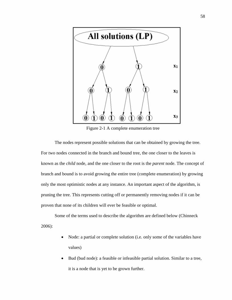
58

Figure 2-1 A complete enumeration tree

The nodes represent possible solutions that can be obtained by growing the tree.

For two nodes connected in the branch and bound tree, the one closer to the leaves is

known as the child node, and the one closer to the root is the parent node. The concept of

branch and bound is to avoid growing the entire tree (complete enumeration) by growing

only the most optimistic nodes at any instance. An important aspect of the algorithm, is

pruning the tree. This represents cutting off or permanently removing nodes if it can be

proven that none of its children will ever be feasible or optimal.

Some of the terms used to describe the algorithm are defined below (Chinneck

2006):

Node: a partial or complete solution (i.e. only some of the variables have

values)

Bud (bud node): a feasible or infeasible partial solution. Similar to a tree,

it is a node that is yet to be grown further.

59

Leaf: a complete solution in which the values to all the variables are

known.

Bounding function: is the optimistic estimator of the objective function

value at a bud node. The function overestimates or underestimates, if the

aim is to maximize or minimize the objective function, respectively.

Branching: is the process of growing a child node from a bud node.

Incumbent: the current best complete feasible solution found.

In order to avoid complete enumeration, the algorithm must define policies with

regards to selecting the next node to be grown, the next variables, how to prune, and

termination criteria for the algorithm. These policies must be defined before solving

integer problems with branch and bound algorithms.

There are three common policies for the next node to be grown: best first, depth

first, and breadth first. The best first approach selects the bud node with best bounding

function value on the tree. The depth first approach selects only from new sets of bud

nodes just created. This policy is usually used when the tree is very deep and integer

solutions are rare. The breadth first grows bud nodes in the same order in which they are

created. This policy is usually used if the analyst is aware that the solution is not far from

the root node. Other methods include the sum of integer infeasibilities, best estimate

using pseudo-costs and best projection.

The variable selection policy determines the next variable to be chosen in order to

create the child node of a bud node. A simple approach is to select the variables in their

natural order (1x ,

2x ,3x ), although an efficient policy can be tailored to the optimization

problem. Some of the policies that have been implemented included the most/least

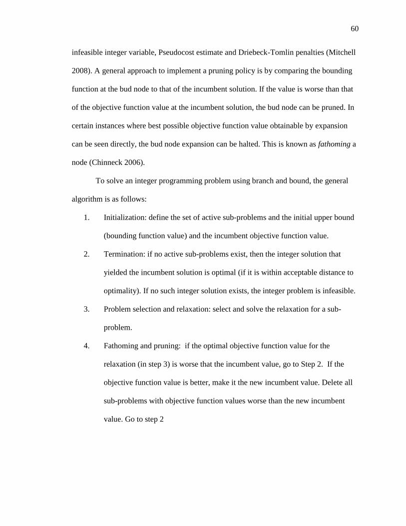
60

infeasible integer variable, Pseudocost estimate and Driebeck-Tomlin penalties (Mitchell

2008). A general approach to implement a pruning policy is by comparing the bounding

function at the bud node to that of the incumbent solution. If the value is worse than that

of the objective function value at the incumbent solution, the bud node can be pruned. In

certain instances where best possible objective function value obtainable by expansion

can be seen directly, the bud node expansion can be halted. This is known as fathoming a

node (Chinneck 2006).

To solve an integer programming problem using branch and bound, the general

algorithm is as follows:

1. Initialization: define the set of active sub-problems and the initial upper bound

(bounding function value) and the incumbent objective function value.

2. Termination: if no active sub-problems exist, then the integer solution that

yielded the incumbent solution is optimal (if it is within acceptable distance to

optimality). If no such integer solution exists, the integer problem is infeasible.

3. Problem selection and relaxation: select and solve the relaxation for a sub-

problem.

4. Fathoming and pruning: if the optimal objective function value for the

relaxation (in step 3) is worse that the incumbent value, go to Step 2. If the

objective function value is better, make it the new incumbent value. Delete all

sub-problems with objective function values worse than the new incumbent

value. Go to step 2

61

5. Partitioning: partition a constraint set of the problem into multiple sub-

problems. Each new sub-problem is bounded by the new incumbent solution.

Go to Step 2

Although the branch and bound algorithm is better than full enumeration, it is not

very efficient in solving problems with a large number of possible solutions. The

algorithm still evaluates too many solutions. One of the challenges faced by the branch

and bound algorithm is the availability of integer feasible solutions during execution.

Since pruning is only possible after obtaining a fathomed solution (Step 4 requires an

incumbent solution), when integer solutions are not readily available pruning a node

becomes impossible. Thus, branch and bound can fail to find an optimal solution due to

inadequate memory as a result of excessive accumulation of active nodes (Lee and

Mitchell 2000).

These limitations of the branch and bound algorithm are overcome when used in

conjunction with cutting planes in the branch and cut algorithm.

2.4.1.2. Branch and cut algorithm. Developed in the 1950s, the cutting plane

method is a convex mathematical technique used to solve integer and mixed integer

linear programming problems. A cutting plane is a linear inequality, in that is generated

(when needed) in the course of solving an integer linear program problem as a sequence

of linear programs (Lee 2004). The computational complexity of the branch and bound

method can be improved immensely by implementing cutting planes at the root node or at

every leaf node. For the past decades, general inequalities such as the Gomory cutting

planes, Knapsack problems based cutting plane, Fenchel cutting planes and the lift and

project cutting planes have been developed that prove useful for most problems (Mitchell

62

2009). The general framework of the cutting plane method for solving an integer linear

program is as follows:

1. Define the linear programming (LP) relaxation of the integer problem

2. Solve for the optimal extreme-point solution (x*) of LP

3. If the solution in step 2 (x*) is all integer subject to existing constraint,

terminate the algorithm because it is optimal.

4. If the solution is not optimal, find an inequality that is satisfied by all feasible

solutions of the ILP, but violated by the extreme-point solution (x*). Add on

the inequality to LP, and go back to Step 1.

The optimal solutions to the LP problem become a sequence of upper bounds on

the optimal value of the integer problem as cutting planes are successively added on. The

most challenging aspect of this method is finding valid cutting planes. By incorporating

the cutting plane method into the branch and bound method, the branch and cut algorithm

becomes:

1. Initialization: define the set of active sub-problems and the initial upper bound

(bounding function value) and the incumbent objective function value.

2. Termination: if no active sub-problems exist, then the integer solution that

yielded the incumbent solution is optimal. If no such integer solution exists, the

integer problem is infeasible.

3. Problem selection: select and delete sub-problem from active set.

4. Relaxation: solve the relaxation for a sub-problem. If the problem is infeasible

go to Step 6, otherwise if it is feasible, add the solution of the sub-problem to

the set of feasible solutions.

63

5. Add cutting planes: if needed, search for cutting planes (inequality) that are

violated by the feasible solution to the sub-problem. If found add it to the LP

relaxation of the sub-problem and return to Step 4 (solve the problem again).

6. Fathoming and pruning: if the optimal objective function value for the

relaxation is worse that the incumbent value, go to Step 2. If the objective

function value is better, make it the new incumbent value. Delete all sub-

problems with objective function values worse than the new incumbent value.

Go to step 2

7. Partitioning: partition a constraint set of problem (select node for expansion)

into multiple sub-problems. Each new sub-problem is bounded by the

incumbent solution. Go to Step 2

A simple two variable example is used to illustrate the branch and cut algorithm

(Mitchell 2002). Consider the integer problem in Equation (2-16) .

1 2-6 5 Min z x x

(2-16)

1 23 11 subject to x x

1 2- 2 5 x x

1 2, 0, int x x eger

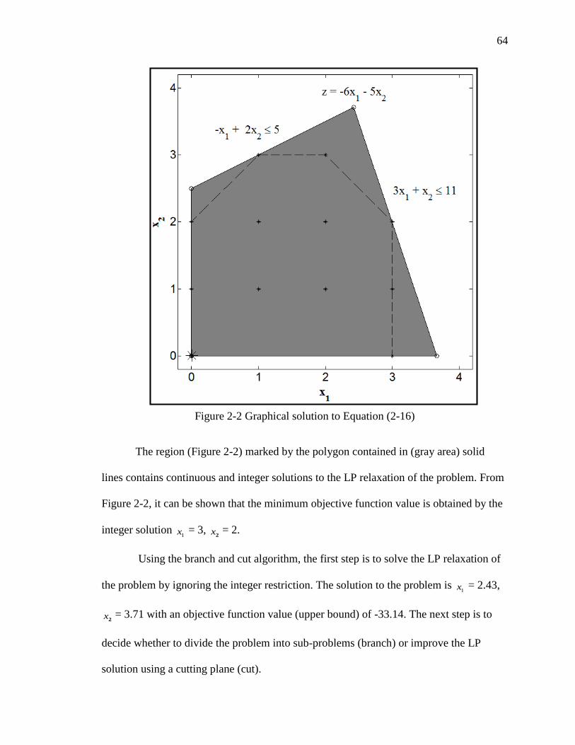
64

Figure 2-2 Graphical solution to Equation (2-16)

The region (Figure 2-2) marked by the polygon contained in (gray area) solid

lines contains continuous and integer solutions to the LP relaxation of the problem. From

Figure 2-2, it can be shown that the minimum objective function value is obtained by the

integer solution 1 x = 3,

2 x = 2.

Using the branch and cut algorithm, the first step is to solve the LP relaxation of

the problem by ignoring the integer restriction. The solution to the problem is 1 x = 2.43,

2 x = 3.71 with an objective function value (upper bound) of -33.14. The next step is to

decide whether to divide the problem into sub-problems (branch) or improve the LP

solution using a cutting plane (cut).

65

Dividing the problem on 1 x result in the following sub-problems: Equation (2-17)

and Equation (2-18) with solutions of 1 x = 3,

2 x = 2 and 1 x = 2,

2 x = 3.5, respectively.

The objective function values are -28 and -29.5, respectively.

Sub-problem 1: 1 2min -6 5 z x x

(2-17) 1 23 11 subject to x x

1 2- 2 5 x x

1 3

x

1 2, 0, int x x eger

Sub-problem 2: 1 2min -6 5 z x x

(2-18)

1 23 11 subject to x x

1 2- 2 5 x x

1 2 x

1 2, 0, int x x eger

66

The first integer solution is obtained by solving sub-problem 1, which now

becomes the incumbent solution. Sub-problem 2 needs to be solved further to determine

if a better integral solution can be obtained since its bounding function value is lower

than the incumbent solution. A cutting plane is implemented to improve the LP solution

for sub-problem 2. A valid cutting plane will be violated by the solution 1 x = 2,

2 x = 3.5

but satisfied by all integer feasible solutions in sub-problem 2. A new sub-problem (Sub-

problem 3) is obtained by adding such a cutting plane.

Sub-problem 3: 1 2min -6 5 z x x

(2-19)

1 23 11 subject to x x

1 2- 2 5 x x

1 2 x

1 22 7 x x (Cutting plane)

1 2, 0, int x x eger

The solution to the LP relaxation of sub-problem 3 is 1 x = 1.8,

2 x = 3.4 with an

objective function value of -27.8. The optimal value obtained from the LP relaxation of

sub-problem 3 is greater than the current incumbent solution. That is, any integer solution

67

obtained from sub-problem 3 will be worse than the current incumbent solution. The

incumbent solution, is therefore, the solution to the original integer problem.

2.4.2. Generating Valid Cutting Planes. As explained earlier, the most

challenging aspect of the branch and cut algorithm is how to generate valid cutting planes

for the particular problem. For a general integer LP solver, valid cutting planes have to be

generated for all possible integer LP problems. There are some methods available for

doing that. However, these cutting planes may not be the best cutting planes to ensure

efficient solution for any particular problem (e.g. integer LP problem of mining

production sequencing) since they do not take into account the peculiar characteristics of

the problem. Nonetheless these cutting planes are useful because they are implemented in

commercial integer optimization solvers (e.g. CPLEX), which are used to solve most

optimization problems. The common cutting plane methods (including Chvátal-Gomory

cutting planes, cutting planes based on polyhedral theory and lift and project cutting

planes) are discussed below.

Chvátal-Gomory cutting planes were initially developed by Gomory (1958) using

the simplex tableau. The convergence to an optimal solution was very slow and made the

approach numerical instable. Chvátal (1973) introduced and implicitly described the

concept of integer rounding. Integer rounding entails combining the linear inequalities of

the current linear programming relaxation subject to the integer variables. The positive

inequality constraints of the problem are summed up and the coefficient of the resulting

constraints rounded down to the nearest integer. To obtain a convex hull11 of feasible

11Convex hull of a set is the smallest convex (non-intersecting) polygon that contains all

the points in the set (Goutsias 2006).

68

integer points, the number of iterations needed is known as the Chvátal rank. The

Chvátal-Gomory cutting plane is the most common cutting plane implemented in branch

and cut algorithms.

One of the main contributions towards solving integer problems using the cutting

plane method was the introduction of polyhedral theory in the 1980s, which allows the

generation of strong cutting planes. The polyhedral theory is based on the implementation

of cutting planes that use the facets of the convex hull of integer feasible points as cuts.

Facets are faces of a polytope12 with one less dimension than that of the polytope. In the

example given in Figure 2-2, all the dashed lines are facets. If the convex hull of all

integer feasible points is known, the integer problem can be solved as an LP problem that

minimizes the objective function over the convex hull.

Other cutting planes have been proposed based on various ideas relating to integer

optimization problems. Some of the common ones include knapsack problem based,

Fenchel and lift and project cutting planes. The knapsack problem is a single constraint

optimization problem. Most integer programming problems can be formulated as

combinations of multiple Knapsack problems. The method entails generating facets and

strong cutting planes for the Knapsack problems and adding them as cutting planes to the

LP relaxation of the integer problem (Mitchell 2009). The Fenchel cutting plane method

solves the separation problem rather than the traditional method of using explicit

knowledge of the polyhedral structure of the problem. The cutting plane excludes the

12 Polytopes are geometrical figures with flat sides bounded by portions of planes, lines,

or hyperplanes. It exists in any number of dimensions. A polygon is a 2-dimensional

polytope (Coxeter 1973).

69

feasible solution of the current sub-problem without excluding the convex hull (Boyd

1994). Lift and project cutting planes involve generating of higher dimensional

representations of the convex hull (lifting) that is projected back to generate multiple

cutting planes. The aim is to reduce the size of the LP needed to generate the cutting

plane (Balas et al. 1993).

2.4.3. Role of Pre-Processing in Efficiency of Branch-and-Cut Algorithm. In

most cases finding integer solutions to the LP relaxation can be cumbersome. Research to

date has demonstrated that a large scale real-world integer problems cannot be solved

without using some form of heuristics or pre-processing approaches. Pre-processing

approaches are often used to convert fractional solutions to integer solutions that result in

the pruning of other sub-problems (Guignard 2010). Many pre-processing techniques in

the literature are implemented before initiating the branch and cut algorithm. This

includes simply eliminating implicit slack variables (removing empty columns and rows),

removing redundant constraints, strengthening bounds on each constraint (right-hand-side

vector), coefficient reduction, aggregation and the use of specialized cuts (Mitchell

2009). The most common pre-processing techniques currently used in mining are the

aggregation (Topal 2008, Boland et al. 2009, Askari-Nasab et al. 2010) and specialized

cutting plane technique (Bley et al. 2010). In this research, the effect of block

aggregation and specialized cutting planes on computational complexity were

investigated for the room and pillar mine sequencing problem.

The aggregation approach is such that multiple variables can be combined as one,

which minimizes the size of the constraints matrix, as well as the number of integer

70

(binary) variables. This is possible if satisfying the bounds on some variables implies

satisfying the bounds of other variables. However, not all variables have this property and

can satisfy this condition. Consequently, the solution to the integer problem may vary

significantly from the optimal solution depending on the size of the aggregates and

aggregation method used. Ramazan (2007) reduces the number of binary variables from

37, 800 to 4,920 using the aggregation approach. He solved the problem, which could not

otherwise be solved in 36 minutes. Ramazan et al. (2005) aggregated ore and waste

blocks to decrease the number of binary variables in the integer programming model. The

block aggregation was performed using a mathematical programming approach to

minimize loss of information pertaining to each block. Boland et al. (2009) introduced a

disaggregation approach in conjunction with block aggregation to solve the production

scheduling problem. The authors realized that block aggregation, which is often referred

to as “binning,” minimizes the size and computational time of the problem. However, in

all these cases, the aggregation strategy affects the optimal solution and many authors

have called for further research to determine optimal aggregation strategy (Askari-Nasab

et al. 2010)

Specialized cutting planes can be added to the problem to eliminate sub-problems

that the analyst knows are sub-optimal. This approach requires in-depth knowledge of the

problem and the nature of optimal solutions to the problem. For example, mine engineers

are aware of sections of the mine (such as the development area) that has to be mined in

specific periods over the planning horizon. A specialized cutting plane can be included to

eliminate solutions that do not mine such blocks in an expected period. Chvátal-Gomory

cutting planes can be formulated from existing active constrains (such as the precedence

71

and production constraints) to eliminate infeasible sub-problems. For example, Bley et al.

(2010) solved the open pit production scheduling problem presented by Caccetta and Hill

(2003) using cutting planes generated by combining the production and precedence

constraints into precedence constrained knapsack problems. The authors noted the

decrease in solution time when cutting planes are implemented. This approach shows real

potential to reduce the computational times associated with mine production sequence

optimization.

This approach is not possible for generalized integer optimization solvers because

it requires intimate knowledge of the particular optimization problem. However, for a

specific problem (e.g. room and pillar mine production sequencing problem) it is a viable

strategy to reduce the computational time required to solve the problem. The most

challenging aspect of this idea is the time it takes to generate the cutting plane.

Specialized cutting planes are efficient if the computational time required to construct

and apply the cutting planes are more than compensated for by the savings in solution

times of the problem (Bley et al. 2010). This research explores the effect of different

specialized cutting planes, specific to underground mining operations on the solution

time.

72

3. APPLICATION OF DISCRETE EVENT SIMULATION IN OPTIMIZATION

COAL MINE ROOM AND PILLAR PANEL

3.1. INTRODUCTION

This chapter focuses on the use of discrete event simulation to determine the

optimal panel width that increases productivity and minimizes cost. An approach is

presented based on simulation experiments to accomplish this goal. An existing room and

pillar coal mine in Illinois was used as a case study to demonstrate the practical

application of the approach.

One of the most important aspects of selecting an optimal panel design is the rate

at which coal is extracted. A smaller panel width may result in a faster extraction (higher

productivity13) if all other parameter are optimal for the selected width. For an existing

mine, selecting a smaller or larger panel width may reduce the productivity, if the

existing fleet size is not optimal for the system. Too large a fleet in the system (due to a

small panel width) results in longer queues and higher waiting times leading to under-

utilization of the haulage fleet. However, a less than optimal number of cars will also

under-utilize the CM. The width of the coal panel should, therefore, be selected to

optimize the productivity given specific mining conditions.

The panel width also affects the unit cost of operation (which includes all fixed

costs and variable costs incurred during production). Some of the costs associate with

R&P production systems include, the operating cost of the shuttle car, continuous miner

(CM), belt feeder, as well as cost associated with roof support. As the width of the panel

changes so does the cost incurred to extract a unit of coal. For example, larger panels

13 Productivity is the rate of output (material production) per unit input in a period.

73

result in longer tramming distances and increased ground control requirements resulting

in higher fuel, maintenance and labor costs.

Current methods (e.g. pressure arch concept) used to determine panel width are

primarily based on geotechnical properties (such as over burden thickness, pillar shape

and size), especially, when pillar recovery is a consideration (Standridge and Nicholas

2012, Luo 2015). Most engineers use experience and practical experimentation to select

the optimal panel width or optimize other aspects of the production process such as the

haulage system to maximize productivity. While these factors are essential in panel

design, it is important to optimize the productivity and unit cost as a function of panel

width at the initial stage of mine design. This should be done rigorously to ensure the

selected panel width maximizes productivity or minimizes unit costs, given all other

constraints.

3.2. FRAMEWORK FOR PANEL WIDTH OPTIMIZATION USING DES

Ultimately, optimizing a design parameter is an optimization problem as

described by Equation (3-1). The decision variable, vector x , represents variables that

affect the objective function f x . Possible values that these variables can take make up

the set of feasible solutions (alternative designs).

minimize

subject to

f

x

x

(3-1)

In the case of panel width design, the objective function could reflect the desire to

maximize mining recovery and productivity as well as minimize unit operating costs.

74

This work focuses on the dual objective of maximizing productivity and minimizing unit

costs. Decision variables can be panel width, cut sequences, the number of continuous

miners (CMs), and the number of haulage units assigned to each CM.

If the objective function can be written mathematically (explicit) in terms of the

decision variables and all constraints can be described similarly, there are many

techniques to solve such optimization problems. Often, however, the objective function is

highly nonlinear and implicit.14 In such cases, simulation is one of the very few

techniques that can solve the problem (Kleijnen 1998). In the case of panel width

optimization, productivity and unit costs associated with cutting, loading, and hauling as

a function of the panel width, equipment fleet, and cut sequence are nonlinear and

implicit. DES offers a means to estimate the unit cost and productivity for a given panel

width, equipment fleet, and cut sequence.

The approach taken in this work is to:

1. Build a valid DES model of the coal loading and hauling operations;

2. Determine a feasible set of decision variable values (panel widths, fleet, and cut

sequences);

3. Estimate objective function values (productivity and unit costs) for each

possible solution from the feasible set; and

4. Select the optimal solution based on the objective function to reflect relative

importance of productivity and unit costs.

14 An implicit objective function, as used here, refers to an objective function that cannot

be expressed as a function of variables in a particular time step alone. Such functions

require knowledge of the variables at multiple time steps. See, for instance, Zou (2012).

75

Generally, simulation optimization methods are used to find the best input

variable values from all possible values (the feasible set) without explicitly analyzing

each possibility. Common simulation optimization methods currently used for system

optimization include the gradient search method, stochastic approximation, response

surfaces methodology, heuristic methods, and statistical methods (Carson and Maria

1997). Response surface and gradient based methods are designed to solve optimization

problems with continuous variables. The decision variables of the panel width

optimization problem (number of entries/panel width, number of cars, and cut sequence)

are discrete and cannot be solved using continuous-based methods.

Statistical methods (e.g. ranking and selection) are computationally exhaustive.

These methods evaluate all system alternatives instead of a finite set. The methods are

also limited to only small problems since they examine the entire feasible set.

Heuristic and metaheuristic (such as simulated annealing and genetic algorithm)

methods can be used to optimize discrete stochastic problems. The development of

computer simulation software has significantly minimized the complexity and time

needed to solve large optimization problems. DES software generally adopts

deterministic metaheuristic optimization algorithms such as tabu search and genetic

algorithm to solve discrete optimization problems with minimal analytical effort. In

contrast, metaheuristic algorithms (e.g. genetic algorithm and simulated annealing)

converge too slowly for practical application.

The panel width optimization problem is complex with each estimate of the

objective function requiring significant time (each estimate requires running the

simulation model for the required number of iterations). The use of algorithms such as

76

genetic algorithm and simulate annealing will require extensive effort to develop

computer codes and application program interface (API) to ensure the optimization

algorithm can interact with Arena®, which is the estimator of the objective function

values.

In this work, the author fully enumerates all possible solutions in the feasible set

because this approach is not very time consuming, in this case. The problem is well

constrained using engineering judgment. For example, it is impractical to mine a 15 entry

panel using one shuttle car, therefore, this option will be excluded from the feasible set.

Once that is done, the feasible set contains tens of combinations rather than hundreds or

thousands. For instance, in the particular case of the case study, the feasible set contains

36 combinations. For situations where the feasible set is large, an optimization algorithm

may be useful. This should be explored in future work.

In this study, the objective function is a dual objective function made up of

productivity and unit cost. To find the optimal solution, one would have to determine the

relative significance of productivity and unit cost to the decision. Since this varies from

one situation to another, the researcher chose not to attempt finding a single optimal

solution, but to present a discussion of results relative to productivity and unit costs. In

situations where this can be done, an objective function (Equation (3-2)) can be

formulated for such situations. The coefficients (η1 and η2) should be selected to scale the

units as well as describe the relative importance of the two objectives.

1* 2* F x productivity unit costs

(3-2)

77

3.3. CASE STUDY

A case study of an actual coal mine is presented in this section to illustrate the

approach discussed in Section 3.2. The discussion here follows the general steps of the

approach as discussed in Section 3.2. The discussion of the simulation modeling (Step 1)

is presented following the major steps of a typical simulation study (Kelton and Sturrock

2003).

3.3.1. Step 1: Build Valid DES Model.

3.3.1.1. Problem formulation. The objective of the panel width optimization

study is to evaluate the impact of panel width on the unit cost and productivity of an

underground R&P operation. A DES model with variables that characterize the coal

cutting, loading and hauling system was built using Arena®. The model predicts unit

mining cost and productivity at different panel widths using user specified cut sequences

and fleet. The DES model was validated with shift production data obtained from a R&P

coal mine in Illinois. The defined performance metric was that the relevant simulated

output should be within 15% of actual values from the mine.

3.3.1.2. System and simulation specification. The mine used for this study is

located in southern Illinois. The mine produces approximately 7 million tons of coal per

year from the Herrin No. 6 seam using R&P mining methods with a panel recovery rate

of 54%. Eight Joy Model 14CM27 CMs (two for each panel) cut and load coal at up to

40 tons per minute with a maximum cutting height of 11.2 ft. Coal is hauled from CMs to

feeder-breakers by 20-ton Joy Model BH20 battery-powered haulage units. A feeder-

breaker is located at the center of each production panel to transfer mined coal from

haulage units to conveyor belts. As the panel advances, the feeder-breaker is moved

forward in three-crosscut increments. The full width of the panel is mined in six-crosscut

78

increments. The panel is mined by first advancing (mining) the center of the panel ahead

of its flanks. The mine has experimented with different panel widths and mining

sequences. Currently, the strategy of advancing the central 11 or 13 entries before

mining rooms on the flanks is the most common. Minimum and maximum panel widths

are 11 and 23 entries, respectively. During normal operations, each CM mines up to

seven entries on one side of a panel.

The objective of the simulation is to develop a valid DES model that predicts unit

mining costs and productivity. Also, the model should provide basic animation for

verification. Input data used in the model were obtained from time studies done at the

mine (Figure 3-1 to Figure 3-6). Raw data were analyzed to fit statistical distributions

using the Chi-squared goodness-of-fit test as shown in Table 3-1. Input data include

loading and dumping times, payloads, and battery change data, which are sampled from

the distributions. Model output includes production per shift, tons per hour, total

operating costs including equipment costs, and the calculated cost per ton for a given

panel width.

Figure 3-1 Haulage unit dumping time

Figure 3-2 Empty haulage unit travel

speed

79

Figure 3-3 Loaded haulage unit travel speed

Figure 3-4 Loaded haulage unit travel

time

Figure 3-5 Haulage unit spotting time

Figure 3-6 CM travel time between cuts

Table 3-1 Input data

Data (s) Distribution(s) P- value

Payload (ton) 12 -

Empty speed (ft s-1) 6.11 + GAMM (0.327, 4.97) < 0.005

Loading time (s) 28 + ERLA (3.63, 3) < 0.005

Dumping time (s) 6 + GAMM (2.79, 5.36) < 0.005

Battery change (s) TRIA (5,7,10) < 0.005

Loaded speed (ft s-1) 6 + GAMM (0.261, 4.24) < 0.005

Time between cuts (s) NORM (797, 87.7) < 0.005

Spotting time (s) 12.5 + GAMM (4.22, 2.11) < 0.005

80

3.3.1.3. Model formulation: CM and haulage logic. The DES modeling

framework requires the entities, resources, and processes of the system to be specified by

the analyst. To initiate the model, entities go through defined processes in a logical

manner waiting for needed resources to become available at each process (i.e. resources

are “busy” if they are being used by other entities) before they go through the process.

The CM is modeled as a resource used for the loading process and can only load one

haulage unit at a time. Loads of coal are modeled as entities with specific attributes

(entity number, payload, and cut sequence – the cut sequence was assigned to each entity

to ensure the information is available to “route” loads to the active cut). Battery-powered

haulage units are modeled as guided transporters used for hauling loads (entities). A

guided transporter is an Arena®-specific modeling construct for material haulage

(Rockwell Automation Inc. 2012). Transporters use entries and crosscuts as haulage

routes, which are modeled to restrict traffic flow such that any point on a haulage route

can only accommodate one haulage unit at a time since the mine openings are not wide

enough for them to pass each other. The feeder-breaker is also modeled as a stationary

resource used for dumping loads (entities). The feeder-breaker and each cutting face are

modeled as stations, which are points in the model where transporters transfer entities.

Haulage routes between stations are modeled as network links to capture varying haulage

distances. Distances for each network link are an input to the model. Figure 3-7 shows

the logic used to model the system.

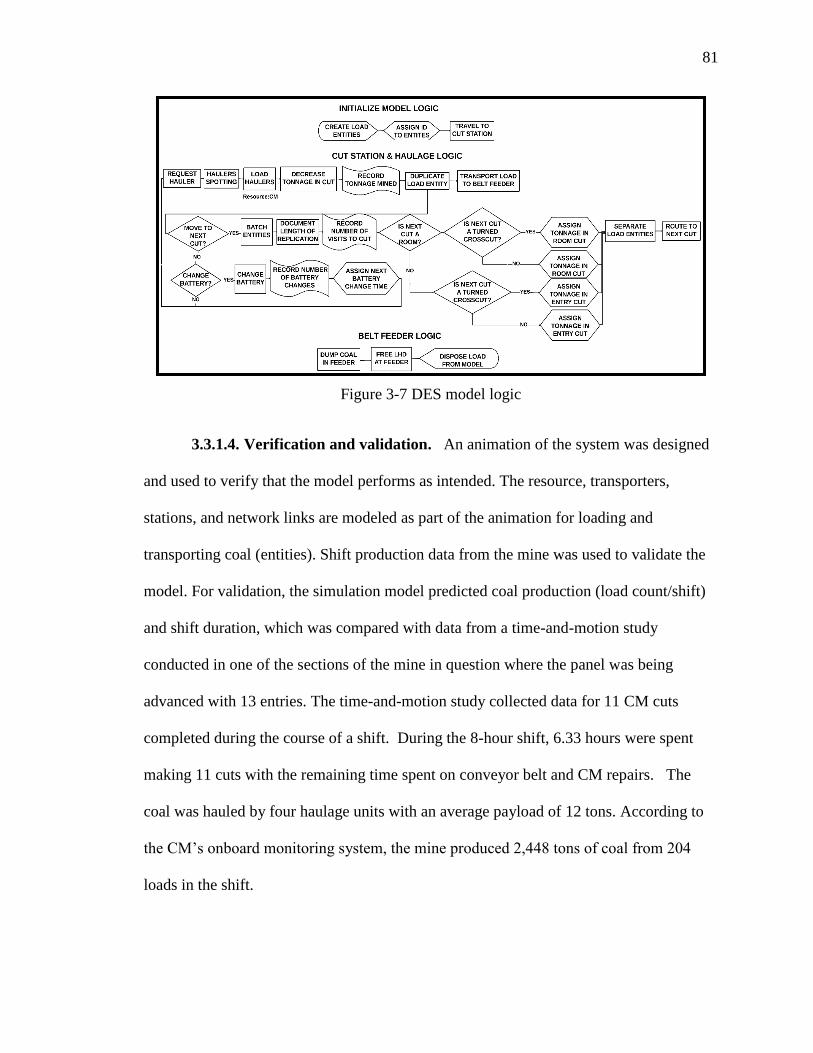
81

Figure 3-7 DES model logic

3.3.1.4. Verification and validation. An animation of the system was designed

and used to verify that the model performs as intended. The resource, transporters,

stations, and network links are modeled as part of the animation for loading and

transporting coal (entities). Shift production data from the mine was used to validate the

model. For validation, the simulation model predicted coal production (load count/shift)

and shift duration, which was compared with data from a time-and-motion study

conducted in one of the sections of the mine in question where the panel was being

advanced with 13 entries. The time-and-motion study collected data for 11 CM cuts

completed during the course of a shift. During the 8-hour shift, 6.33 hours were spent

making 11 cuts with the remaining time spent on conveyor belt and CM repairs. The

coal was hauled by four haulage units with an average payload of 12 tons. According to

the CM’s onboard monitoring system, the mine produced 2,448 tons of coal from 204

loads in the shift.

82

In the validation experiment, 150 replications were conducted to obtain estimates

of load count and total coal production, mining duration, and other output. The number of

replications was selected such that the half-width15 of the mining duration (the most

uncertain output) is less than 1% of the estimated duration. The cut sequence used in the

validation experiment duplicated that used during the time-and-motion study. Each

replication stops when all specified cuts have been mined in the simulation.

Table 3-2 shows the results of the validation experiments for the production shift.

The model takes a bit longer (30 minutes more) to mine the 11 cuts and also loads 24

more haulage units than the observed system. The key performance measures are the

number of loads mined from the 11 cuts and the duration of mining, which are within

11% and 8%, respectively, of the actual values. Both values are within the 15% specified

earlier. The model was thus deemed valid and used for all the experiments.

Table 3-2 Results of validation experiment

Parameter Actual Simulated Difference

Duration of mining (hours) 6.33 6.83 8%

Production (tons) 2,448 2,748 12%

Number of haulage unit loads 204 226 11%

Half-width of duration (hours) -- 0.012 --

15 Half-width = 1,1 /2n

st

n ,

1,1 /2nt = critical values from t tables, n = number of

replications, s = sample standard deviation.

83

3.3.2. Step 2: Determine Feasible Set. This step is similar to the experimental

design steps in classical simulation studies. The main distinguishing feature is that the

experimental design should cover all possible combinations of the decision variables so

that the entire feasible set is described in the experiments. The decision variables that

affect the objective function (mining cost and productivity) are panel width (number of

entries), number of haulage units assigned to each CM, and the cut sequence. At the

mine, the staff has experimented with cut sequences that advance 11 or 13 entries first

before expanding into rooms, if necessary. Hence, these experiments were to evaluate

whether to advance with 11 or 13 entries before mining rooms leading to two possible

sequences. Each sequence is based on work done by Hirschi (2012) and with specific

input from Dr. J. Hirschi.16 Once the initial advance is mined, the mine has mined

anywhere from zero to five additional rooms on each side depending on the designed

width of the panel. The mine has also experimented with three shuttle cars and is

currently using four shuttle cars in each section. The engineers plan to increase the

number of shuttle cars to five in large panels. To avoid further field experimentation and

account for all previous and planned scenarios, the number of shuttle cars was varied

between three and five in the feasible set.

Hence the experiment includes three factors:

Number of initial entries (11 or 13) for advance;

Number of rooms (0, 1, …, 5 rooms on each side of the panel); and

16 Dr J Hirschi optimized the cut sequences for the panel widths analyzed. He has years

of experience in identifying the optimal sequence for R&P coal mines including the

collaborating mine.

84

Number of haulage units assigned to each CM (3, 4, or 5).

This leads to a total of 2 6 3 36 combinations of experiments that describe

the entire feasible set. For each experiment, 150 replications were run to estimate the

productivity and unit cost. Each replication was run until all cuts in the sequence have

been mined.

The cut sequence was provided as an input based on mining practices at the mine.

Mining faces in the 11- or 13-entry initial advance are mined using the cut sequence

shown in Figure 3-8(a) and (b), respectively. Rooms are mined using optimal cut

sequences based on Hirschi (2012), such as the one shown in Figure 3-9(a) and (b) for a

15-entry panel width. The experiment evaluates a mining system with two CMs (one on

each side of the section). The conveyor belt is located in the center entry of the panel.

Figure 3-8(a) Cut sequence for 11-entry initial advance

85

Figure 3-8(b) Cut sequence for 13-entry initial advance

Figure 3-9(a) Room cut sequence for 11-entry initial advance with two additional rooms

on each side

86

Figure 3-9(b) Room cut sequence for 13-entry initial advance with one additional room

on each side

The simulation output includes production data (e.g. load count and total

production tonnage), duration of mining, and percentage of time the CM spends loading

haulers. Other outputs include total cost of mining and estimated unit costs (Equation

(3-3)).

CUnit costs ($/ton)

Total production

CM CM H H r Fn C n t C

(3-3)

where CMn and

Hn are the number of CMs and haulage units, respectively; rt is

the duration of the simulation run; CMC and

HC are hourly costs for CMs and haulage

units, respectively; and FC is fixed costs, which include labor and equipment for

advancing belt and power systems.

87

3.3.3. Step 3: Estimate Objective Function Values. Table 3-3 shows the results

for all 36 experiments. The table includes the unit cost and productivity for all

combinations of the three factors determined in Section 3.3.2.

Table 3-3 Productivity and unit cost of all 36 simulations

# No. of initial

advance

entries

No. of

additional

rooms

No. of

haulage

units

Productivity

(tons/hour)

Unit cost

($/ton)

1 11 0 3 535 3.33

2 11 1 3 541 3.02

3 11 2 3 540 2.87

4 11 3 3 540 2.70

5 11 4 3 537 2.62

6 11 5 3 534 2.52

7 13 0 3 532 3.08

8 13 1 3 536 2.85

9 13 2 3 534 2.74

10 13 3 3 532 2.61

11 13 4 3 529 2.55

12 13 5 3 525 2.47

13 11 0 4 550 3.29

14 11 1 4 555 2.98

15 11 2 4 556 2.83

88

Table 3-3 Productivity and unit cost of all 36 simulations. Cont.

# No. of initial

advance

entries

No. of

additional

rooms

No. of

haulage

units

Productivity

(tons/hour)

Unit cost

($/ton)

16 11 3 4 558 2.65

17 11 4 4 557 2.56

18 11 5 4 557 2.45

19 13 0 4 549 3.03

20 13 1 4 553 2.80

21 13 2 4 554 2.68

22 13 3 4 555 2.55

23 13 4 4 554 2.48

24 13 5 4 553 2.39

25 11 0 5 550 3.28

26 11 1 5 556 2.97

27 11 2 5 557 2.82

28 11 3 5 559 2.64

29 11 4 5 558 2.55

30 11 5 5 558 2.44

31 13 0 5 549 3.02

32 13 1 5 553 2.79

33 13 2 5 554 2.67

34 13 3 5 555 2.54

89

Table 3-3 Productivity and unit cost of all 36 simulations. Cont.

# No. of initial

advance

entries

No. of

additional

rooms

No. of

haulage

units

Productivity

(tons/hour)

Unit cost

($/ton)

35 13 4 5 554 2.47

36 13 5 5 554 2.38

3.3.3.1. Effect of panel width. Figure 3-10 to Figure 3-17 show simulation

results for experiments with the default number of haulage units (four per CM). These

results indicate the effect of panel width (number of entries) on productivity and unit

cost. Figure 3-10 and Figure 3-11 show that total production and duration of mining

increase with increasing number of entries. This is what one would expect, if the model is

performing well. Figure 3-12 and Figure 3-13 show that the percentage of production

time the CM spends loading haulage units initially increases with increasing panel width

until an optimal panel width is reached. This indicates that there is excess haulage unit

capacity in the system with less than optimal number of entries. CM operations are

inefficient due to the excessive spotting time resulting in long wait times and bunching;

however, expanding panel width beyond the optimal results in inadequate haulage unit

capacity and under-utilization of the CM. This is confirmed by Figure 3-14 and Figure

3-15 showing that the optimal panel width. Initial expansion of the panel reduces the

haulage unit cycle time (minimizes waiting time). However, further expansion of the

panel increases haulage unit cycle times because haul distances become longer, leading to

a haulage unit constrained operation. Adding more haulage units will increase

productivity and CM utilization as discussed further in Section 3.3.3.2.

90

These trends (cycle time and CM loading times) directly result in the observed

trend in productivity (Figure 3-16). Panel widths of 17 and 19 entries result in maximum

productivity when advancing with a base width of 11 and 13 entries, respectively.

However, this trend is not mirrored in the unit cost results (Figure 3-17) due to the effect

of fixed costs that make larger panels more cost effective even with sub-optimal

productivity. In Figure 3-17, unit costs are estimated using Equation (3-3). Hourly costs

of haulage units and CM are estimated at $104.13 and $122.40 (InfoMine 2013)17. Fixed

costs for moving the belt are estimated at $81,050.

The following observations can be made from these results:

Systems which advance initially with 11 entries outperform those that

advance with 13 entries under similar conditions (cut sequences and

equipment);

Haulage unit cycle times correlate very well with productivity and CM

loading times;

There appears to be an optimal panel width for a given number of haulage

units based on productivity analysis; and

Unit costs decrease with increasing number of entries due to the effect of

fixed costs.

17InfoMine cost data is used in this study to protect the mine’s confidential data.

91

Figure 3-10 Total production

Figure 3-11 Duration of mining

Figure 3-12 CM time spent loading (LHS)

Figure 3-13 CM time spent loading

(RHS)

Figure 3-14 Average cycle times (LHS)

Figure 3-15 Average cycle times (RHS)

0

50,000

100,000

11 13 15 17 19 21 23

Pro

du

cton

[to

ns]

Number of entries

11 entry system 13 entry system

0

100,000

11 13 15 17 19 21 23

Pro

du

cton

[to

ns]

Number of entries

11 entry system

13 entry system

24.0

24.5

25.0

25.5

11 13 15 17 19 21 23

Load

ing t

ime

[%]

Number of entries

11 entry system 13 entry system

24.0

25.0

11 13 15 17 19 21 23C

M U

tili

zati

on

[%

]

Number of entries

11 entry system

13 entry system

10.20

10.30

10.40

10.50

11 13 15 17 19 21 23Cyle

tim

e [m

ins]

Number of entries

11 entry system 13 entry system

10.20

10.30

10.40

10.50

11 13 15 17 19 21 23Cyle

tim

e [m

ins]

Number of entries

11 entry system

13 entry system

92

Figure 3-16 Productivity

Figure 3-17 Unit costs

3.3.3.2. Effect of number of haulage units. Figure 3-18 and Figure 3-19 show

the sensitivity of productivity to the number of haulage units. It can be observed that with

the addition of each haulage unit, productivity increases; however, the increase when the

number of haulage units increases from three to four is much more significant than the

increase when the number of haulage units increases from four to five. Also, the number

of haulage units can affect optimal panel width. For example, Figure 3-18 shows that

optimal panel width with three haulage units assigned to each CM is 13 entries, whereas

with four haulage units, optimal panel width is 17 entries. This is because the number of

assigned haulage units affects the width at which the system becomes limited by haulage

unit capacity.

Figure 3-20 and Figure 3-21 show the sensitivity of unit cost results to number of

haulage units. With each additional haulage unit, unit costs increase for both systems 11

and 13 entries in the initial advance.

Based on these results we can observe the results are sensitive to the number of

haulage units as follows:

Productivity increases with additional haulage units, and

540545550555560

11 13 15 17 19 21 23

Pro

du

ctiv

ity [

tph

]

Number of entries

11 entry system 13 entry system

1.40

3.40

11 13 15 17 19 21 23

Co

st p

er t

on

[$/t

]

Number of entries

11 entry system

13 entry system

93

Optimal number of entries changes with varying number of haulage units.

Cost increases outpace productivity increases with each additional haulage unit

leading to higher unit costs.

Figure 3-18 Effect of number of haulage

units on productivity for 11-entry system

Figure 3-19 Effect of number of haulage

units on productivity for 13-entry

system

Figure 3-20 Effect of number of haulage

units on unit costs for 11-entry system

Figure 3-21 Effect of number of haulage

units on unit costs for 13-entry system

3.3.3.3. Effect of fixed costs. From Equation (3-3), if fixed costs are negligible,

the unit cost curve should be the inverse of the productivity relationship. However,

Figure 3-16 and Figure 3-17 do not show this relationship indicating that fixed costs

significantly affect the unit cost relationship. Figure 3-22 shows the sensitivity of the unit

cost relationship to fixed costs using results for the sequences where 11 entries are

advanced initially with four haulage units (same as Figure 3-17). Figure 3-22 shows that

520530540550560

11 13 15 17 19 21

Pro

du

ctiv

ity [

tph

]

Number of entries

3 Cars 4 Cars 5 Cars

520530540550560

13 15 17 19 21 23

Pro

du

ctiv

ity [

tph

]

Number of entries

3 Cars 4 Cars 5 Cars

$2.00 $2.40 $2.80 $3.20 $3.60

11 13 15 17 19 21

Un

it c

ost

s

[$/t

on

]

Number of entries

3 Cars 4 Cars 5 Cars

$2.00 $2.40 $2.80 $3.20 $3.60

13 15 17 19 21 23

Un

it c

ost

s [$

/ton

]

Number of entries

3 Cars 4 Cars 5 Cars

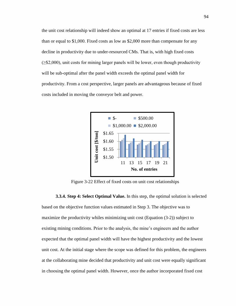
94

the unit cost relationship will indeed show an optimal at 17 entries if fixed costs are less

than or equal to $1,000. Fixed costs as low as $2,000 more than compensate for any

decline in productivity due to under-resourced CMs. That is, with high fixed costs

(≥$2,000), unit costs for mining larger panels will be lower, even though productivity

will be sub-optimal after the panel width exceeds the optimal panel width for

productivity. From a cost perspective, larger panels are advantageous because of fixed

costs included in moving the conveyor belt and power.

Figure 3-22 Effect of fixed costs on unit cost relationships

3.3.4. Step 4: Select Optimal Value. In this step, the optimal solution is selected

based on the objective function values estimated in Step 3. The objective was to

maximize the productivity whiles minimizing unit cost (Equation (3-2)) subject to

existing mining conditions. Prior to the analysis, the mine’s engineers and the author

expected that the optimal panel width will have the highest productivity and the lowest

unit cost. At the initial stage where the scope was defined for this problem, the engineers

at the collaborating mine decided that productivity and unit cost were equally significant

in choosing the optimal panel width. However, once the author incorporated fixed cost

$1.50

$1.55

$1.60

$1.65

11 13 15 17 19 21Un

it c

ost

[$/t

on

]

No. of entries

$- $500.00

$1,000.00 $2,000.00

95

into the analysis of unit cost (Section 3.3.3.3), it became clear that the choice of an

optimal panel width has to be made either by prioritizing productivity or unit cost. Based

on the results, the productivity was deemed more important than unit cost by the mine’s

engineers. Based solely on productivity (i.e. 2 in Equation (3-2) is set to zero), the

revised objective function value increases significantly as the panel width increases until

an optimal value is reached, beyond which the value decreases. For the existing mining

condition, a panel width of 17 entries and an 11-entry initial advance is deemed optimal

to maximize productivity (Table 3-3).

3.4. SUMMARY

This research effort presents an approach, based on discrete event simulation, to

optimize productivity and unit costs as a function of panel width. The 4-step approach

has been successfully illustrated with a case study of a real underground coal mine in

Illinois. The research has successfully built a discrete event simulator that can be used to

facilitate panel width design. The simulator is capable of evaluating the effect of panel

width (number of entries) on R&P mine productivity and unit costs. The simulator has

successfully been validated for the case study mine. The validated model has been used

to evaluate the effect of panel width on productivity and unit costs of the mine.

Based on results of the case study, the following general conclusions can be

made:

For particular operating conditions (equipment, cut sequence, etc.), there

exist an optimal panel width that maximizes productivity.

96

For particular operating conditions, an optimal panel width exists that

minimizes unit costs, only if the fixed costs are negligible. For any

significant fixed cost, larger panels will always result in lower unit costs.

For the cooperating mine, in particular, the following recommendations can be

made:

Mining with sequences that initially advance 11 entries is better than

mining with sequences that advance 13 entries initially.

The optimal panel width under simulated conditions is 17 entries (3 rooms

on each side of the 11-entry base width).

Four (4) haulage units should be assigned to each CM in the panel.

The practice of moving the belt after mining three crosscuts to ensure haul

distances to rooms is reasonable.

97

4. INCORPORATING CHANGING DUTY CYCLES IN CM-SHUTTLE CAR

MATCHING USING DISCRETE EVENT SIMULATION

4.1. INTRODUCTION

The cut sequence used to mine a coal panel in room and pillar mines differ,

depending on production, ground control and ventilation requirements. In most mines, the

direction of mining and cut sequence change as mining progresses, resulting in varying

shuttle car and CM cycle times. Multiple cuts are mined in a single shift with varying

distances from the conveyor belt feeder, as well as from one cut to the other. This results

in frequent tramming by the CM from cut to cut. As the cuts change, so do the cycle

times of the shuttle cars as they travel to and from the belt feeder. The duty cycles may

vary significantly as mining progresses, depending on the cut sequence, which

determines distance from the loading point to the conveyor belt. The CM and shuttle cars

may be underutilized, if changing duty cycles is not accounted for in matching a CM to

an optimal number of shuttle cars.

As shown in Chapter 3, the size of the haulage fleet affects the productivity in a

panel; although a higher number of shuttle cars does not always lead to higher

productivity. Thus, mine managers desire an optimal haulage fleet size that maximizes its

objectives (e.g. productivity) while meeting all constraints. To optimize the haulage fleet

size, it is important to consider the operating cycle of the haulage equipment (including

loading, traveling loaded, dumping, traveling empty and waiting, as necessary).

In coal R&P mining, the duty cycles of production equipment are a function of

the panel width and cut sequence. Modeling and simulation could be used to account for

98

the effect of varying duty cycles in determining the optimal fleet size.18 To capture

varying cycle times in the modeling process, the panels have to be divided into different

segments to discretize the process (otherwise, the analysis has to be done for each

infinitesimal instance in time). The real challenge is how to define the panel segments. If

the segments are too small, they lose practical relevance for mine management.

Alternatively, if the segments are too large, the duty cycles within the segment itself will

vary significantly. Once the segments are defined, the next challenge is how to model and

run simulation experiments for the different segments, as well as optimize the fleet size

for each segment without excess computational cost.

DES can be used to model an operation to predict the resources needed, fleet type

and availability, as well as the current performance of the system. The defined resources

usually include loading and off-loading equipment, maintenance personnel, and other

equipment. The typical input data needed for fleet size optimization models include cycle

times and equipment speed, loading, dumping/delivery and production rates, and travel

distances. The output parameters are dependent on the objective of the optimization.

Typical output variables include queue length, waiting time, resource utilization, duration

of mining, unit cost, and productivity. Longer queue lengths indicate excess equipment

fleet capacity in the system, and vice versa. Similarly, under-utilization of loading and

dumping resources indicate the fleet size is less than optimal. Experiments are conducted,

which typically include varying the size of the fleet and evaluating the impact on the

18 See Section 3.2 for reasons why simulation is a good approach for optimizing

productivity of coal R&P mining in panels.

99

output variables. Determining the optimal fleet size is dependent on a balance between

these variables.

Very limited work can be found in literature that incorporates changing duty

cycles in determining the optimal fleet size for a mining operation. None of these

applications can be found in room and pillar mining, where changes in duty cycle can be

observed frequently. There is no comprehensive approach in the literature that has been

used to evaluate the effect of changing duty cycles on system efficiency in underground

mines.

This chapter focuses on incorporating changing duty cycles in determining the

optimal number of shuttle cars. A modeling approach is presented capable of defining

mining segments that capture changing equipment cycle times in an operation. The

approach is demonstrated and validated using real-life R&P mining data.

4.2. PROPOSED APPROACH

The proposed approach consists of three major components: (1) building a valid

DES model; (2) defining operating segments; and (3) conducting simulation experiments.

These components are described in general here, while a case study is used to illustrate

how to apply the approach in Section 4.3.

4.2.1. Building DES Model. Kelton and Sturrock (2003) describe steps for a

successful simulation analysis. These steps include problem formulation; solution

methodology; system and simulation specification; model formulation and construction;

verification and validation; experimentation and analysis; and documenting, reporting

and dissemination. These steps have been successfully used to optimize mine production

systems (Awuah-Offei et al. 2003, Miwa and Takakuwa 2011, Awuah-Offei et al. 2012,

and Michalakopoulos et al. 2015). This section will take a closer look at the specific steps

100

that are unique when the process is applied to study the effect of duty cycles on optimal

CM-shuttle car matching.

4.2.1.1. Problem formulation. The first step in optimizing any system is

defining and formulating the problem. This includes the system to be simulated,

stakeholder’s expectations, system constraints, and performance metrics used to measure

the quality of the simulated system under study. In this application, the objective is to

determine the optimal number of shuttle cars allocated to a continuous miner in a room

and pillar coal mining system while accounting for varying duty cycles (continuous miner

and shuttle car). For a model to accomplish these objectives, it should be capable of

predicting the output(s) that are used in the optimization decision (i.e. the model should

be able to serve as the objective function). These could be the same objectives used for

other fleet optimization but these outputs need to be sensitive to the duty cycle, otherwise

they will not achieve the objective. For example, productivity is suitable for evaluating

the performance of the material handling system in a particular section of an underground

mine, whereas production may not be. This is because the production (total amount of ore

that can be mined from that section) is fixed but the rate at which the mining is done is

affected by different fleets. Other suitable outputs can be mining duration (time to

complete mining of a particular section), queue length, utilization of loading equipment,

and unit costs.

4.2.1.2. Model formulation and construction. Understanding and defining the

system specification makes it easier for an analyst to visualize and design a simulation

model that meets the set objectives. Generally, the model constructed for fleet

optimization in mining includes the loading, hauling and dumping logic. The loading and

101

dumping equipment are defined as resources and the hauling equipment as entities or

transporters (an Arena® modeling construct for material handling applications). The

loading resource is under-utilized if there are fewer than optimal cars in the system and

vice versa. In this application, the modeling approach should be such that, the model is

capable of evaluating the sensitivity of the output variables to changing duty cycle times.

For example, the time it takes to mine different segments in the coal panel using the same

fleet size will be longer in sections with higher cycle times. To account for changing duty

cycle in optimizing the number of shuttle cars, it may be necessary to develop different

models for each segment of the panel. It is also important to take into account the cut

sequence, haul routes and distances unique to each segment. The analyst should be able

to conduct necessary experiments efficiently using the constructed model.

4.2.2. Defining Operating Segments. The duty cycles of the CM and shuttle

cars change mainly because of the cut sequence (i.e. the CM has to keep changing where

loading occurs), although one could argue they change continuously. Without defining

segments, the optimal fleet size has to be defined for each infinitesimal instance in time

where there is a significant difference in duty cycle. Hence, defining segments is

necessary to discretize the problem for meaningful analysis. It is ideal that the duty cycles

within a segment remain near constant (otherwise, you have the same problem as the

panel). However, the different segments should also capture the changing duty cycles as

mining progresses in the panel. In other words, intra-segment variation in duty cycles is

undesirable whereas inter-segment variation is acceptable.

Defining too many segments (e.g. each cut is a segment) is computationally

expensive and practically meaningless for mine management (i.e. engineers and foremen

102

cannot allocate a different number of shuttle cars for each cut). Defining too few

segments (e.g. two segments) would result in segments where the duty cycles vary

significantly within the segment. This defeats the purpose of this sort of analysis. The

optimal number and size of segments, is somewhere between these two extremes. Also,

for an existing mine, the segments have to be defined such that using variable fleet sizes

will not significantly change the allocation or dispatch practices at the mine. For

example, if the segments are defined so that it is optimal to change the number of cars in

the middle of a shift, this will result in operational delays, equipment underutilization or

personal scheduling challenges. Therefore, a good rule of thumb would be to select

segments that start at the time when fleet assignments are made. This is usually at the

beginning of a shift. This is the approach taken in this research.

After establishing a guiding principle for determining segment sizes (e.g.

segments that coincide with shifts), it is still not trivial to determine the number and size

of segments. Especially in cases where the mine or panel is being planned and no data

exists on how long it takes to mine a cut or certain number of cuts. Two approaches are

suggested for existing and planned operations. For existing operations, an analyst can

examine the number of cuts the crew typically mines in a shift and use that to define the

size of a segment. For planned operations, the same simulation model that will be used

for the segment-by-segment fleet analysis should be used to simulate the entire segment

first. The simulation results can then be used to determine the average number of

segments mined in the period it will take to complete a shift (e.g. eight hours). The first

approach is illustrated by the case study in Section 4.3.

103

4.2.3. Simulation Experiments. Experimental analysis is an essential step that

allows the analyst to evaluate and identify optimal scenarios that maximizes the system

efficiency. In fleet sizing, the primary experimental factor is the size of the fleet. The

number of experiments conducted is a function of the current fleet size being used, as

well as stakeholder’s expectations. Usually the analyst, evaluates the sensitivity of the

defined simulation output to decreasing and/or increasing fleet size in the system. In most

experiments, if there is no significant change to the output when the number of cars is

increased (or decreased), the analyst does not introduce additional cars in the system. To

account for changing duty cycles of production equipment, a generalized model is

defined that incorporates all cuts and distances in the system for a particular panel width.

By doing so, the only input that changes in the model is the cut sequence. The validated

model can be replicated without developing new models for each segment. The process

analyzer tool in Arena® can be used to vary the number of cars in the system without

manually changing it in the model. In order to take advantage of the process analyzer

tool, the number of cars in the model is defined as a variable in Arena® along with an

initial value. The output for each experimental scenario can simply be obtained by adding

the range of fleet sizes to be evaluated.

4.3. CASE STUDY

A case study of a coal mine is used to illustrate the approach presented in Section

4.2. The case study is presented using the same outline as the proposed approach.

4.3.1. Building DES Model. A detailed description of the simulation model of

the system in this case study can be found in Chapter 3. This section provides a summary

description with emphasis on the unique aspects relating to accounting for the changing

duty cycle as mining progresses through the panel, which is not addressed in Chapter 3.

104

The studied mine is a room and pillar coal mine in Illinois. The mine mines coal

from the Herrin Number 6 seam with eight Joy Global 14CM27 continuous miners for

cutting and loading (with up to two CMs for each panel). Each CM loads up to 40 tons

per minute of coal with a maximum cutting height of 11.2 ft. The mine produces

approximately 7 million tons of coal per year with a panel recovery rate of 54%. The

mine uses 20-ton Joy Global BH20 battery operated shuttle cars to haul the cut coal from

the mining cut to a conveyor belt feeder. The conveyor belt feeder is located at the centre

of each production panel and moved forward every three crosscuts. The optimal panel

width recommended for operation, based on the study presented in Chapter 3, is 17

entries with a fleet of two CMs, each assigned four shuttle cars. The recommended fleet

is optimal for mining the entire panel and does not account for variations in duty cycle as

mining progresses.

The input data used in the model was obtained from time and motion studies done

at the mine, as well as data from equipment monitoring systems. The raw data was

analyzed to fit statistical distributions using the Chi-squared goodness-of-fit test. The

model input data includes spotting, loading and dumping times, payload and battery

change data. (The data is presented in Section 3.3.1.2.)

As explained in Chapter 3, the CM is modeled as a resource used for the loading

process and can only load one shuttle car at a time. The truck loads of coal are modeled

as entities with specific attributes (entity number, payload, and cut sequence). The shuttle

cars are modeled as guided transporters used for hauling the loads (entities). The

conveyor belt feeder is also modeled as a resource needed to dump the load entities. The

belt feeder and the cuts are modeled as stations. To capture the varying haulage distances,

105

the haulage routes between stations are modeled as network links. The distance for each

network link is an input to the model. Figure 3-7 (on page 81) shows the logic used to

model the cutting, loading and haulage practices of the mining system.

The cut sequence (Figure 4-1 and Figure 4-2) was provided as an input based on

mining practices at the mine. Since the analysis in this chapter only focuses on the

optimal panel width from Chapter 3 (17-entries wide), only the optimal cut sequence for

the optimal panel width (found to be the cut sequence based on Hirschi (2012) where 11

entries are initially advanced before mining the three additional entries on each side -

Figure 4-1 and Figure 4-2) is considered in this analysis. Mining cuts in the 11 entries at

the center of the panel are mined using the cut sequence shown in Figure 4-1. Rooms in

the remaining 6 entries are mined using the cut sequence shown in Figure 4-2.

Figure 4-1 Cut sequence for the 11 entries at the center of the panel

The simulation output includes duration of mining, cycle times, average

waiting time in loading queue, productivity (tons per hour) produced and percentage of

time the CM spends loading cars.

106

Figure 4-2 Cut sequence for the three additional entries on each side

As presented in Chapter 3, the model was validated using coal production data

collected from a representative eight-hour shift at the mine. During the shift, 6.33 hours

were spent to complete 11 cuts with the remaining time spent on conveyor belt and CM

repairs. The total coal production and mining duration (time it takes to mine the 11 cuts)

predicted by the DES model from the studied shift is compared to the actual data from the

mine. A performance measure of ±15% deviation based on stakeholder’s expectations

was set for this research. The model took a bit longer (30 minutes more) to mine the 11

cuts and also loaded 24 more cars than the observed system. The number of loads mined

from the 11 cuts and the duration were within 11% and 8%, respectively, of the actual

values. Both values were within the 15% specified earlier. The model was thus deemed

valid and used for all the experiments.

4.3.2. Selecting Number of Operating Segments. As discussed in Section

4.2.2, this approach depends on how segments are defined in the analysis. In this case

study, the 17-entry panel is divided into segments of up to 11 cuts each based on the

typical shift used for validation. The goal was to define segments that can be mined in a

shift, since car assignments are made at the beginning of a shift at this particular mine.

107

Only the first six crosscuts of the 17-entry panel, with a total of 146 and 151 cuts on

the left- and right-hand sides of the panel, respectively, were analysed in this work. Six

crosscuts completely mine out the width of the panel using the mines cut sequences

(Figure 4-1 and Figure 4-2). This resulted in a total of 14 mining segments on each side

of the panel with exactly 11 cuts in each, except for the last segment on each side. The

last segment contained three and eight cuts on the left- and right-hand sides, respectively.

Segments 1 to 8 are found in the entries mined with the cut sequence in Figure 4-1.

Segment 9 is mined using both cut sequences and segments 10 to 14 are mined with the

cut sequence in Figure 4-2.

4.3.3. Simulation Experiments and Analysis. Experimental analysis was

conducted using the validated model to determine the optimal number of shuttle cars

required in each panel segment. As at the mine, one CM is assigned to work on each side

of the belt feeder in the panel. In the experiments, the number of shuttle cars assigned to

each CM was varied from one to six. Preliminary analysis indicated that a fleet of more

than six cars assigned to each CM has no further significant impact on the model outputs.

This leads to a total of 84 (14 segments × 6) experiments. For each experiment, 150

replications were run for the analysis.19 Each replication was run until all cuts in the

segment had been mined.

Results of the simulation experiments are discussed in the next section.

4.3.4. Results and Discussions. The simulation results are shown in Figure 4-3 to

Figure 4-7. Figure 4-3 shows the duration of mining in each segment using variable

19 As in Chapter 3, the number of replications was selected to ensure that the half-width

of the mining duration is less than 1% of the estimated duration.

108

number of shuttle cars. As expected, the tonnage in each segment is mined out at a slower

pace with fewer than optimal cars. Duration of mining starts to decrease significantly,

initially as the fleet size is increased, until it reaches an optimal value, beyond which

further increases in the number cars results in no significant reduction in the time it takes

to mine out the segment. This correlates well with the utilization of the CM for loading

shuttle cars (Figure 4-6. In segments 1, 2, and 7, the duration of mining approaches a

constant after a fleet size of three. There is no significant change in the duration of

mining when the number of cars increases from three to four. For the remaining

segments, a constant value is reached after four shuttle cars are used in the system. The

duration of mining increases by 41 minutes on average when the number of cars increases

from three to four. This is because the average distances from the cut to the belt feeder in

segments 1, 2 and 7 are relatively short compared to other segments.

Figure 4-4 shows the effect of varying fleet size on the average cycle time in each

segment. The overall average cycle time increases as the number of shuttle cars increases.

This correlates well with the waiting time in the loading queue (Figure 4-5). As the

number of cars increase, the cars wait longer in queue to be loaded and therefore, the

overall cycle time is increased. Figure 4-6 shows that the average percentage of

production time the CM spends loading the shuttle cars, as opposed to tramming or

waiting on cars, in each segment. The time spent loading increases with the increasing

number of shuttle cars, until an optimal fleet size is obtained. This indicates that there is

limited haulage unit capacity in the system at the beginning and, therefore, the CM is

under-utilized. Once an optimal number of cars is reached, any additional car results in

inefficient CM operations (over-matched). Excess cars in the system results in longer

109

waiting times and no productivity gains. There is no significant change in the CM

utilization after an optimal fleet size is reached. In Segments 1, 2, and 7 the percentage of

production time spent loading the shuttle cars approaches a constant after a fleet size of

three. For the remaining segments a constant value is reached after four shuttle cars are

used in the system. The same trend can be seen in the productivity (Figure 4-7) as the

number of cars changes from one to six. There is no significant change in productivity as

the number of shuttle cars is increased from three to four in Segments 1, 2, and 7. For the

remaining segments, increasing the fleet size from three to four increases the productivity

by 5% on average.

By accounting for changing duty cycle in selecting the optimum fleet size for the

CM-shuttle car mine system, the optimal number of cars needed to mine the 17-entry

panel reduces as compared to the estimate determined in Chapter 3. The analysis done in

Chapter 3 shows that it is optimal to mine the 17-entry panel with 8 shuttle cars (four cars

for each CM) at all times. Incorporating changing duty cycle times in the fleet size

optimization analysis suggests that the mine can meet its productivity target using six

shuttle cars in three out of the 14 segments of the panel. Based on the operating cost

($104.13 per hour) of the battery operated shuttle cars, the overall cost of mining the coal

in segments 1, 2 and 7 decreases by $5,86220 per panel. In addition to significantly

20 The cost to mine each segment was estimated based on the number of cars assigned to

the segment, the unit cost of operating a shuttle car and the duration of mining (Figure 4

3). The duration of mining was 9.04, 9.58 and 9.53 hours for segments 1, 2, and 7,

respectively. The cost of mining segment 1 is estimated to be $5,646 and $7,529 using 3

and 4 cars per CM, respectively. The cost of mining segment 2 is estimated to be $5,984

and $7,979 using 3 and 4 cars per CM, respectively. The cost of mining segment 7 is

estimated to be $5,955 and $7,940 using 3 and 4 cars per CM, respectively.

110

reducing the operating cost, this analysis allows equipment which will otherwise be

underutilized in segments 1, 2 and 7 to be freed up for other activities. Accounting for

changing duty cycles in determining the optimal fleet size needed for mining, especially

at the early stages of investment minimizes capital cost and avoids unnecessary

expenditure. The results of this study demonstrates that the fleet size needed for an

operation can be overestimated if changing duty cycles is not accounted for.

111

Figure 4-3 Duration of mining for all segments for varying number of cars

0

10

20

1 2 3 4 5 6Du

rati

on

[h

rs]

# of cars

Segment 1

0

10

20

1 2 3 4 5 6

Du

rati

on

[h

rs]

# of cars

Segment 2

0

10

20

1 2 3 4 5 6Du

rati

on

[h

rs]

# of cars

Segment 3

0

10

20

1 2 3 4 5 6Du

rati

on

[h

rs]

# of cars

Segment 4

0

10

20

1 2 3 4 5 6

Du

rati

on

[h

rs]

# of cars

Segment 5

0

10

20

1 2 3 4 5 6Du

rati

on

[h

rs]

# of cars

Segment 6

0

10

20

1 2 3 4 5 6Du

rati

on

[h

rs]

# of cars

Segment 7

0

10

20

1 2 3 4 5 6Du

rati

on

[h

rs]

# of cars

Segment 8

0

10

20

1 2 3 4 5 6Du

rati

on

[h

rs]

# of cars

Segment 9

0

10

20

1 2 3 4 5 6Du

rati

on

[h

rs]

# of cars

Segment 10

0

10

20

1 2 3 4 5 6

Du

rati

on

[h

rs]

# of cars

Segment 11

0

10

20

1 2 3 4 5 6Du

rati

on

[h

rs]

# of cars

Segment 12

0

10

20

1 2 3 4 5 6Du

rati

on

[h

rs]

# of cars

Segment 13

0

10

20

1 2 3 4 5 6Du

rati

on

[h

rs]

# of cars

Segment 14

112

Figure 4-4 Average cycle time for all segments for varying number of cars

0

20

1 2 3 4 5 6# of cars

Segment 1

LHS RHS

Cycl

e ti

mes

[m

ins]

0

20

1 2 3 4 5 6C

ycl

e ti

mes

[m

ins]

# of cars

Segment 2

LHS RHS

0

10

20

1 2 3 4 5 6

Cycl

e ti

mes

[m

ins]

# of cars

Segment 3

LHS RHS

0

20

1 2 3 4 5 6

Cycl

e ti

mes

[m

ins]

# of cars

Segment 4

LHS RHS

0

20

1 2 3 4 5 6

Cycl

e ti

mes

[m

ins]

# of cars

Segment 5

LHS RHS

0

10

20

1 2 3 4 5 6# of cars

Segment 6

LHS RHS

Cycl

e ti

mes

[m

ins]

0

20

1 2 3 4 5 6# of cars

Segment 7

LHS RHS

Cycl

e ti

mes

[m

ins]

0

20

1 2 3 4 5 6# of cars

Segment 8

LHS RHS

Cycl

e ti

mes

[m

ins]

0

20

1 2 3 4 5 6

# of cars

Segment 9

LHS RHS

Cycl

e ti

mes

[m

ins]

0

20

1 2 3 4 5 6

Cycl

e ti

mes

[m

ins]

# of cars

Segment 10

LHS RHS

0

10

20

1 2 3 4 5 6

Cycl

e ti

mes

[m

ins]

# of cars

Segment 11

LHS RHS

0

20

1 2 3 4 5 6

Cycl

e ti

mes

[m

ins]

# of cars

Segment 12

LHS RHS

0

20

1 2 3 4 5 6

Cycl

e ti

mes

…

# of cars

Segment 13

LHS RHS

0

20

1 2 3 4 5 6C

ycl

e ti

mes

[m

ins]

# of cars

Segment 14

LHS RHS

113

Figure 4-5 Average car waiting time in queue at CM for all segments for varying number of cars

0246

1 2 3 4 5 6

Wait

ing t

ime

[min

s]

# of cars

Segment 1

LHS RHS

0246

1 2 3 4 5 6

# of cars

Segment 2

LHS RHS

Wait

ing t

ime

[min

s]

0246

1 2 3 4 5 6

Wait

ing t

ime

[min

s]

# of cars

Segment 3

LHS RHS

0

2

46

1 2 3 4 5 6

# of cars

Segment 4

LHS RHS

0

2

4

6

1 2 3 4 5 6

# of cars

Segment 5

LHS RHS

0

2

4

6

1 2 3 4 5 6

# of cars

Segment 6LHS RHS

0246

1 2 3 4 5 6

# of cars

Segment 7

LHS RHS

0246

1 2 3 4 5 6

# of cars

Segment 8

LHS RHS

0

2

4

6

1 2 3 4 5 6

# of cars

Segment 9

LHS RHS

0

2

4

6

1 2 3 4 5 6

# of cars

Segment 10

LHS RHS

0246

1 2 3 4 5 6

# of cars

Segment 11

LHS RHS

Wa

itin

g t

ime

[min

s]

0246

1 2 3 4 5 6

# of cars

Segment 12

LHS RHS

Wait

ing t

ime

[min

s]

0246

1 2 3 4 5 6

# of cars

Segment 13

LHS RHS

Wait

ing t

ime

[min

s] 0

2

4

6

1 2 3 4 5 6

# of cars

Segment 14

LHS RHS

Wait

ing t

ime

[min

s]

114

Figure 4-6 Percentage of time CM spent loading shuttle cars for all segments for varying number of cars

0

20

40

1 2 3 4 5 6

CM

Uti

l [%

]

# of cars

Segment 1

LHS RHS

0

20

40

1 2 3 4 5 6C

M U

til

[%]

# of cars

Segment 2

LHS RHS

0

20

40

1 2 3 4 5 6

CM

Uti

l [%

]

# of cars

Segment 3

LHS RHS

0

20

40

1 2 3 4 5 6

CM

Uti

l [%

]

# of cars

Segment 4

LHS RHS

0

20

40

1 2 3 4 5 6

CM

Uti

l [%

]

# of cars

Segment 5

LHS RHS

0

20

40

1 2 3 4 5 6

CM

Uti

l [%

]

# of cars

Segment 6

LHS RHS

0

20

40

1 2 3 4 5 6

CM

Uti

l [%

]

# of cars

Segment 7

LHS RHS

0

20

40

1 2 3 4 5 6C

M U

til

[%]

# of cars

Segment 8

LHS RHS

0

20

40

1 2 3 4 5 6

CM

Uti

l [%

]

# of cars

Segment 9

LHS RHS

0

20

40

1 2 3 4 5 6

CM

Uti

l [%

]

# of cars

Segment 10

LHS RHS

0

20

40

1 2 3 4 5 6

CM

Uti

l [%

]

# of cars

Segment 11

LHS RHS

0

20

40

1 2 3 4 5 6

CM

Uti

l [%

]

# of cars

Segment 12

LHS RHS

0

20

40

1 2 3 4 5 6

CM

Uti

l [%

]

# of cars

Segment 13

LHS RHS

0

50

1 2 3 4 5 6C

M U

til

[%]

# of cars

Segment 14

LHS RHS

115

Figure 4-7 Productivity for all segments for varying number of cars

0

200

400

600

1 2 3 4 5 6

# of cars

Segment 1

Pro

du

ctiv

ity [

ton

/hr]

0

200

400

600

1 2 3 4 5 6

# of cars

Segment 2

0

200

400

600

1 2 3 4 5 6

# of cars

Segment 3

0

200

400

600

1 2 3 4 5 6

# of cars

Segment 4

0

200

400

600

1 2 3 4 5 6

# of cars

Segment 5

0

200

400

600

1 2 3 4 5 6

# of cars

Segment 6

0

200

400

600

1 2 3 4 5 6

# of cars

Segment 7

0

200

400

600

1 2 3 4 5 6

# of cars

Segment 8

0

200

400

600

1 2 3 4 5 6

# of cars

Segment 9

0

200

400

600

1 2 3 4 5 6

# of cars

Segment 10

0

200

400

600

1 2 3 4 5 6

# of cars

Segment 11

Pro

du

ctiv

ity [

ton

/hr]

0

200

400

600

1 2 3 4 5 6

# of cars

Segment 12

Pro

du

ctiv

ity [

ton

/hr]

0

200

400

600

1 2 3 4 5 6

Pro

du

ctiv

ity [

ton

/hr]

# of cars

Segment 13

0

100

200

300

1 2 3 4 5 6

# of cars

Segment 14

Pro

du

ctiv

ity [

ton

/hr]

116

4.4. SUMMARY

A simulation approach is proposed to investigate whether the shuttle car fleet size

used to mine a particular panel width is optimal in different segments of the panel. The

proposed approach includes criteria used to define segments that reflect changing

equipment cycle times. The research also includes experimental analysis that minimizes

computational cost and evaluate the effect of changing duty cycles on the productivity,

cycle times and the duration of mining. The results indicate that, for particular operating

conditions (equipment, cut sequence, etc.), the optimal fleet size is different for different

segments of the panel. Changes in haul distance and cut sequence affect the optimal

number of cars required in each segment. The total distance travelled by the shuttle cars

in segments 1, 2, and 7 is shorter than the remaining segments. Therefore, fewer number

of cars are needed to mine these segments. For the mining system evaluated and the

defined segments, a fleet size of four shuttle cars is optimal for 80% of the segments

(Table 4-1). An optimal fleet size of three is observed for the remaining segments. The

mine can dispatch the excess shuttle cars to other areas of the operation, once these

segments are scheduled to be mined. Otherwise, the mine can continue to use four cars

for all segments, if the change in the actual unit cost by adding a shuttle car is minimal

compared to the gain in productivity.

Table 4-1 Optimal number of shuttle cars in each segment

Segment Coal tonnage in Segment Optimal fleet size

1 5,437 3

2 5,158 3

117

Table 4-1 Optimal number of shuttle cars in each segment. Cont.

Segment Coal tonnage in Segment Optimal fleet size

3 4,740 4

4 4,182 4

5 5,018 4

6 5,158 4

7 4,740 3

8 4,740 4

9 4,529 4

10 5,403 4

11 5,117 4

12 5,117 4

13 4,971 4

14 1,754 4

118

5. A DETERMININSTIC FRAMEWORK FOR INCORPORATING RISK IN

ROOM-AND-PILLAR MINE PRODUCTION SEQUENCING USING BILP

5.1. INTRODUCTION

Linear programming (LP) is one of the main optimization tools used for mine

production sequencing. The ability to model complex systems with a variety of

constraints makes LP versatile compared to other mathematical models. In mine

production sequencing, researchers most often define the decision variables as the

proportion of a block mined in a period. In most cases, a block is either mined completely

in a particular period or not at all. If this constraint is imposed on the decision variables

of the LP problem, the resulting problem is a binary integer linear programming (BILP)

problem. A BILP model is an integer LP model in which each decision variable can only

take on a value of zero or one. Modeling the many activities associated with mine

production sequencing as binary integer variables subject to strict sequencing

requirements, results in large and complex problems which are NP-hard.21 As a result,

past modeling attempts only solve large-scale sequencing problems in a limited time

frame (Newman and Kuchta 2007). Other researchers relax this constraint (binary integer

variables) for some of the decision variables leading to mixed integer linear programming

(MILP) problems (Gershon 1982, Barbaro and Ramani 1986, Askari-Nasab et al. 2010,

Eivazy, and Askari-Nasab 2012). However, such models can lead to infeasible solutions

(solutions in which a block is mined over several time periods) that require sub-optimal

post-processing to be meaningful for mining.

21 A problem is NP-hard if an algorithm for solving it can be converted into one for

solving any NP-problem (nondeterministic polynomial time) problem (Weisstein 2009).

119

In this chapter, a BILP approach instead of an MILP one is used in order to assure

practically feasible solutions. (The BILP model is compared to an MILP one to evaluate

the effect of block precedence constraints on solution complexity.) The objective of this

study is to develop a deterministic BILP model that is capable of incorporating multiple

mining risks while maximizing the net present value (NPV) of the operation. The model

is referred to as a “long-term” production sequencing model because NPV is often not as

important in short-term sequencing. It is important to note that the model can solve any

number of time periods so long as NPV and/or risk are the desired objective functions.

The disadvantage of this approach is that the resulting problem is more difficult to solve.

The optimization problem is solved using the CPLEX (IBM, Armonk, NY) solver

through the CPLEX API for Matlab®. A simulated lead room and pillar (R&P) mine data

set is used to verify the model and demonstrate the ability to model multiple mining risks

as BILP. The modeling of mining risk is based on the stochastic modeling approach by

Dimitrakopoulos and Ramazan (2004) used to characterize uncertainty in open pit mine

production sequencing. Block aggregation techniques are used to minimize the

computational complexity22 associated with solving these sequencing problems.

5.2. MODELING R&P PRODUCTION SEQUENCING AS BILP

The objective of the BILP model is to maximize the overall net present value of

the R&P operation and minimize the discounted value of risk while meeting all

constraints. In the context of this study, risk is defined as the probability of a block

property deviating (in an undesirable way) from the desired property. There are two

22 In this work, computational complexity is used to refer to how difficult a problem is to

solve and it is measured with computational time and the number of iterations required to

solve the problem.

120

important aspects to modeling the discounted value of risk: risk cost penalty and discount

rate of risk. Conceptually, the risk cost penalty is the extra cost needed to take recourse.

For example, for geotechnical risks, the risk cost penalty will be the cost for additional

support (on top of what is planned), if the actual geotechnical property is ‘worse’ than

predicted. For ore grade, it will be the cost to ensure the period’s metal production target

is met. For the case study solved in this work, grade and geotechnical risks are used to

verify that BILP can be used to model multiple mining risks. The discount rate of risk is

applied to discount the risk cost penalty. It has the practical effect of deferring mining of

high risk blocks till later periods and reduces risk since more data (knowledge) may

become available, which will reduce the risk associated with mining such blocks.

The notations used in defining decision variables, parameters, and constraints are

defined in the nomenclature.

5.2.1. Objective Function. Equation (5-1) is a dual objective function model that

maximizes the NPV and minimizes the discounted cost of risk in each mining period. The

model defines separate variables for mining rooms as well as pillars. The discounted

profit depends on the market priceip of the ore mined, the recovery

ir , tonnageit , average

grade of each blocku

iq , and the unit cost of miningtc . The model incorporates pillar

extraction as an integral part of determining the optimal NPV. This is important in metal

room-and-pillar production sequencing where high grade ore is left in support pillars.

121

(1 ) (1 )

1

t tt i i i t i k k k ke it ktt t

i t k t

NPV

i it i i k kt k ki t k t

r t

r

Discounted

p r t q c tp r t q c tMax w x y

d d

R x c t R y c t

wd

risk

(5-1)

5.2.2. Constraints. Equations (5-2) to (5-7) are basic constraints needed to obtain

a feasible production sequence. Combined, these result in (I + K + J) ∙ T decision

variables and (T +1) ∙ (I + K + J) + T ∙ (A + U) constraints.

, ,

,

( )   ,i

l u

t tit k kt

i k

R r x r y R t

(5-2)

  '  

1 1

 0        ,i

T T

i it i t

t i O t

N x x i t

(5-3a)

'

  '   '  

1 , 1

'

     0   ,ik

k kt i t k t

t i k O t

T T

N y x y k t

(5-3b)

' '

  '  

1 1

 0 ,j

jt j t

t j O t

T T

jN z z j t

(5-3c)

  1,           

T

i

t

tx i

(5-4a)

122

  1,            

T

t

kty k

(5-4b)

  1,            

T

t

jtz j

(5-4c)

(  )   

,i k

l uMR x

ty MR t

it ktt i kt t

(5-5)

( )   , , ,

  ,      ,( )   

,

q x q yi kit ktl i k u

q q tt tx y

it kti k

(5-6)

' ,s

it j t jx z i O t

(5-7a)

' ,s

kt j t jy z k O t

(5-7b)

5.2.2.1. Resource constraint. Equation (5-2) constrains the model from

exceeding available resource capacity (Rtα,u) or under-utilizing available resources (Rt

α,l)

in a particular period. This results in T (number of scheduling periods) constraints for

each modeled resource leading to a total of A·T constraints. Mining resources may

include production and development equipment, labor, and other auxiliary equipment

required to extract the material being mined. Mine haulage truck fleet is the only resource

used in the case study in Section 5.4 to validate this constraint.

123

5.2.2.2. Precedence constraint. Equation (5-3) constrains block and pillar

mining precedence, which is the single most significant contributor to the problem’s

complexity (Bienstock and Zuckerberg 2010). The equation results in (I+K+J)∙T

constraints ensuring that a block, pillar, or section cannot be mined until the set of blocks,

blocks and pillars, or sections that restrict access to it are all mined first. This constraint

allows for practical mining of blocks, pillars, and sections. For each block, pillar, and

section, a set {Oi, Oik, Oj} of blocks, blocks and pillars, and sections, respectively, are

defined to be mined prior to its extraction. To minimize the complexity and number of

constraints, the mine is divided into sections, which could be a section of the mine, or

other aggregate of blocks and pillars as appropriate for mine planning purposes.

It is entirely possible to use only block-pillar constraints (Equation (5-3a) &

(5-3b)) alone to model this problem. However, this will make each block constraint

complex with all preceding blocks included in the constraint. By including the section

precedence constraint in Equation (5-3c), along with block-pillar precedence in Equations

(5-3a) and (5-3b), the complexity of each constraint is reduced (reduce the number of

decision variables in each constraint). That is, with the exception of blocks in the same

section as the block under consideration, all other blocks preceding the block, which are

in other sections, can be represented by just the section decision variables. In instances of

the problem where all three constraints are used, the section decision variables were

modeled as continuous (as opposed to binary) variables, which allows for partial mining

of sections in a period and selectivity of mining blocks. By defining section decision

variables as continuous, the model becomes a mixed integer linear program.

124

This study explores ways to solve the R&P sequencing problem without the

block-pillar constraints (Equations (5-3a) & (5-3b)) in order to save computational time.

To accomplish this, the section precedence constraints (Equation (5-3c)) can be used

without the block-pillar precedence constraints by adding a block-in-section constraint

(Equation (5-7)). This constraint is written such that when a section is mined, all the

blocks in that section are mined as well. In this instance of the problem, all block, pillar

and section decision variables are defined as binary variables. Then the problem can be

formulated without the block-pillar precedence constraints. In that case, the block

precedence constraints constitute only J·T constraints instead of (I+K+J)·T constraints.

However, this adds on an additional (I + K)·T block-in-section constraints (see Section

5.2.2.6 for details).

5.2.2.3. Reserve constraint. Equation (5-4a) to (5-4c) are reserve constraints,

which ensure that the ore reserve mined at the end of a time period is less or equal to the

available reserve. When a block or pillar is mined in a particular period, it cannot be

mined in other periods. This constraint results in (I+K+J) constraints.

5.2.2.4. Mining rate constraint. Equation (5-5) ensures that the total tonnage of

material mined in each period is within production targets (t

uMR and l

tMR ). The

constraint is such that upper and lower limits can be set on production targets for each

period, if necessary. This constraint controls the mining rate and results in T constraints.

5.2.2.5. Quality constraint. Equation (5-6) ensures that the solution meets

quality requirements. For each quality property of interest, there is a separate equation.

Quality properties of interest include grades and deleterious elements or minerals content.

Each set will result in T constraints to ensure that average constituents (grade and

125

contaminants) mined in a period are within the desired range ( ,lqt and ,u

qt ) for that

period. Thus, this results in a total of U·T constraints. This constraint forms a basis for

blending and quality control. The case study problem solved in this work does not

account for multiple metals which sometimes occur, in commercial quantities, with lead

mineralization. Only lead grades are considered in the case study.

5.2.2.6. Block-in-section constraint. Equation (5-7) ensures that once a section

is scheduled for mining, all blocks in the section are mined in the same period. This

constraint is used only when block and pillar precedence constraints (Equations (5-3a)

and (5-3b)) are not used in the model. For it to work properly, all decision variables have

to be binary. This results in (I+K)∙T constraints, compared to (I+K+J)∙T block-pillar

precedence constraints.

5.3. SOLUTION FORMULATION

Equations (5-2) to (5-7) are solved using the CPLEX solver through the CPLEX

API for Matlab®. The CPLEX software uses branch and cut search to solve discrete

optimization problems. A generalized binary or mixed integer linear program is

formulated mathematically in the form of Equation (5-8). Inputs required by CPLEX are

the cost (or benefit) coefficient vector ( c ), generated from the objective function; the

equality constraint matrix ( eqA ); the inequality constraint matrix ( A ); and limits (right

hand-side of constraint equations) of inequality and equality constraints ( b and eqb ),

respectively. The CPLEX solver also requires other constraints on decision variables

(integer, binary, etc.).

126

min

:

eq eq

z cx

subject to

b

A x

Ax b

(5-8)

11

1

11

1

11

1

Vector of decision variables

T

IT

T

KT

T

JT

x

x

x

y

y

y

z

z

z

x

11

1

11

1

Vector of cost coefficient

0

0

0

x

x

T

x

IT

y

y

T

y

KT

c

c

c

c

c

c

c

.. . . .

1 1

it

r

r

it i ix

it ei t i

t ti ti t

R cp r t q c tw

d dc w

. . . . .

1 1

k kt

r

r

t k k t i

tk t

ky

kt e t

k t

p r t q c t R cw

dc

dw

From Equation (5-1), elements of c are present values of blocks less the

discounted risk penalty associated with mining these blocks in a particular period. Hence,

the length of c is the number of decision variables. The solution algorithm developed by

the author in this research allows the user to provide a set of blocks and time periods,

block properties (grades, tonnages, etc.), discount rates, risks, and other input, which the

algorithm uses to generate the vector c , as shown above. The solution algorithm also

creates constraint matrices using information provided by the user. Equation (5-7) results

127

in an equality constraint used to formulate eqA and eqb in Equation (5-8). All other

constraints are inequality constraints. For each constraint, the solution algorithm needs to

formulate a matrix which becomes part of A in Equation (5-8) and a right-hand side

(RHS) vector, which becomes part of b in Equation (5-8).

The solution algorithm is implemented in Matlab® version R2014a and consists

of a master function and various other sub-functions, which are used to formulate a

specific cost coefficient vector or constraints. The Matlab® program is set up so that the

user can provide the amount of each resource required to mine each block and the total

resource available in each period. Thus, resources can be controlled for the life of the

mine to maintain a feasible mining schedule and efficient use of resources. To formulate

the mining rate matrix, the algorithm requires the tonnage of material in each block and

the production demand for each period. The program requires the user to provide

information on the blocks and pillars in each section. The program also requires the user

to provide the average grade or deleterious material content of each block and limits on

them for each period. Thus, the user can set upper and/or lower limits on grades and

others for each period. The precedence constraint requires users to provide indices for

each block and pillar, or section. For each block, the set of blocks that precede it are in

the same sections (there is no need to add blocks from other sections because sections are

added to the precedence sets). A set of indices are used to describe each section such that

sections that precedes another section can be mined first. All inequality constraint

matrices and RHS vectors are concatenated into a single matrix and a single vector.

Along with the cost coefficient vector, these serve as input for the CPLEX solver.

128

The algorithm then calls the CPLEX solver via the CPLEX Matlab API. Once a

solution is obtained from CPLEX, the solution is post-processed to obtain a meaningful

sequence and a visual plot of the solution.

5.4. CASE STUDY

5.4.1. Case Study Problems. A simulated data set was used in this paper to

verify and illustrate the model and solution algorithm. A geologic block model of lead

mineralization was created with geostatistical methods using the Geovia Surpac®

software. The mineable reserve in the model was determined using a regular (spacing of

pillars) room-and-pillar lead mine design. The mining system is simulated as a single-

level lead room and pillar operation. Figure 5-1 shows the mine layout and the simulated

lead grades.

Each mining block was assigned geologic attributes including the grade, grade

risk and geotechnical risk. The data was exported to text files as input along with block

indices for the BILP model. The verification problem included 2,361 blocks, each

containing approximately 250 tons of ore. The production sequencing problem did not

account for primary developments such as drift development. The problem did not

include pillar recovery, although the model is capable of solving problems with pillar

recovery. The project and risk discount rates may vary depending on the situation and

management’s tolerance for risk. For this case study, the cash-flows and risks costs were

discounted at 8% and 5%, respectively.

129

(a)

(b)

Figure 5-1 Case study: (a) mine layout, colored to illustrate sections; (b) grade

distribution

Other input data needed to verify the model is shown in Table 5-1. The problem

evaluated risk associated with lead grades and rock strength (geotechnical risk).

Table 5-1 Model input data

Parameter Value Parameter Value

cost of mining ($/ton) 19.96

Resource capacity per period

(loads) 2,192

lead price ($/kg) 1.70 Minimum production (ton/period) 32,857

Unit cost of risk (grade, $/ton) 15.40 Maximum production (ton/period) 53,571

Unit cost of risk

(geotechnical, $/ton) 7.60 Number of sections 42

Discount rate (economic) 8% Recovery (overall) 90%

Discount rate (risk) 5% lead target (cutoff) 3.2%

Block tonnage (ton) 250 lead grade (mean) 6.2%

Resource capacity per block

(loads) 13 Block grade std. dev. 1.59%

130

The verification problem included 42 sections. Table 5-2 shows the section

precedence used in the examples. The section precedence is defined such that parallel

mining of sections is feasible and respects the development plan (Figure 5-1). The block

precedence data is too large to show in this section.

Table 5-2 Section precedence constraint

Section

#

Precedence

Set

Section

#

Precedence

Set

Section

# Precedence Set

1 { } 15 {3} 29 {17,18,24,25,26,27}

2 {1} 16 {} 30 {17,18,24,25,26,28}

3 {1,2} 17 {} 31 {17,18,24,25,26,27}

4 {1,2,3} 18 {17} 32 {17,18,24,25,26,28,30}

5 {4,27}

19 {20,21}

33 {17,18, 24,25,26,27,

29,31}

6 {5}

20 {19,21}

34 {17,18,24,25,26,

28,30,32,}

7 {5,6}

21 {17,18}

35 {17,18, 24,25,26,27,

29,31,33}

8 {5,6,7}

22 {19,20,21}

36 {17,18,24,25,26,

28,30,32,34}

9 {5,6,7,8}

23 {19,20,21,2

2}

37 {17,18,24,25,26,28,30,3

2,34,36}

10 {5,6,7,8,9 }

24 {17,18}

38 {17,18,24,25,26,28,30,3

2,34,36,37}

11 {5,…,10}

25 {24}

39 {17,18,24,..,27,29,31,33

,35}

12 {11,13}

26 {17,18, 25}

40 {17,18,24,..,27,29,31,33

,35,39}

13 {5,…,11}

27 {17,18,24,2

5,26}

41 {19,..,23,25,26,28,30,32

,36,37,38}

14 {5,..,11,13}

28 {17,18,24,2

5,26}

42 {19,..,23,25,26,28,30,32

,36,37,38,41}

131

The optimization problem was solved using CPLEX version 12.2, with the

Matlab® API, which uses the branch and cut method to solve integer linear programs.

Computational experiments are performed to evaluate the effect of solving the production

sequencing problem with and without the block precedence constraints (note that there

are no pillar precedence constraints because there is no pillar extraction in this case). In

this experiment, the problem is solved for only two periods to illustrate the differences

between the problems.23 In the first scenario, the MILP problem is solved with the block

precedence constraints, which results in 4,722 block binary decision variables, 84

continuous section decision variables and 7,219 inequality constraints. This scenario

allows for the partial mining of sections. Further computational experiments were done to

examine the effect of block precedence on the complexity of the problem. A smaller

precedence set is defined for each block by reducing the number of decision variables in

each constraint. This was done by eliminating some of the blocks in each precedence set.

The effect of reducing the precedence set by up to 32% and 48% on the solution time and

number of iterations was evaluated.

In the second scenario, the problem is solved without the block precedence

constraints. In order to use the block-in-section constraints, all the decision variables are

defined as binary. It does not allow for partial mining of sections; thus each section can

only be mined once in a single period. The problem is thus a BILP problem, which

23 Two periods are used because the point was to illustrate the effect of the constraints. A

simple problem allows one to solve the problem many times in a short period for the

analysis.

132

includes 4,806 binary decision variables, 4,722 equality constraints (block-in-section

constraints) and 2,497 inequality constraints.

In a second set of experiments, the BILP problem (with no block precedence

constraints) is solved for 14 periods. The problem includes 33,642 binary variables,

33,054 equality constraints (block-in-section constraints) and 3,061 inequality

constraints. This problem is more realistic and used to illustrate the ability of the model to

solve realistic mining problems. Two instances of this problem are solved: one where the

ratio of ‘NPV’: ‘grade risk’: ‘geotechnical risk’ is 1:1:1 and another where the ratio is

1:2:2. These instances are used to illustrate the effect these ratios can have on the

solution.

The output data obtained includes, the solution found by the optimization function

(period each block is to be mined in), the optimal objective function value, execution

time of the algorithm, and number of iterations. A gap tolerance of 0.001 is set for the

problem. Both scenarios are run on a 64-bit Dell Precision T5610 computer with twin

quadcore Intel Xeon E5-2609 (2.5 GHz, 10 MB) processors and 32 GB RAM

5.4.2. Results and Discussion. Each solution was verified, after post-processing,

to ensure that the optimal production sequence respects all the constraints. Figure 5-2

shows optimal solutions of the two-period problem used to investigate the influence of

the block-precedence constraints on computational complexity.

Table 5-3 shows the effect of the block precedence constraints on the number of

iterations and CPLEX algorithm’s execution time. By eliminating the 4,722 block

precedence constraints, 97% fewer iterations are required to obtain a solution even

though 4,722 equality constraints are added to the problem and all variables are binary.

133

The computational time required to solve the problem reduced from 2.34 to 0.58 minutes.

This is more than a four-fold reduction in computational time. This trend is probably

going to be the same or worse (i.e. introduction of block precedence will require more

than four times the computational time) for larger problems. Hence, by aggregating

geologic blocks into sections and completely eliminating block precedence constraints,

larger problems can be solved using the BILP in more reasonable time. This is very

important for these kinds of problems because mine engineers tend to run many variants

of the sequencing problem (where input parameters are varied in each instance) in order

to determine the ‘optimal’ sequence. For large problems, with hundreds of thousands of

blocks, the time savings to the mine can be significant.

(a)

(b)

Figure 5-2 Two-period optimal production sequence: (a) with block precedence

constraints; (b) without block precedence constraints.

Table 5-3 Effect of block precedence on computational complexity

134

Percent of

original

variables

in block

precedence

constraints

Precedence constraints Computational

time (mins)

No. of

iterations

Objective

function

value ($)

100% With block precedence

constraints

2.34 36,381 4516.2M

100% Without block precedence

constraints

0.58 966 4515.9M

68% With block precedence

constraints

1.80 6,711 4522.0M

68% Without block precedence

constraints

0.51 683 4526.0M

52% With block precedence

constraints

1.39 6,260 4526.3M

52% Without block precedence

constraints

0.51 983 4526.0M

The effect of the nature of the block precedence constraints on the observation,

that adding block precedences significantly increases computation complexity, was

examined with further experiments. That is, the work examined whether the time savings

is more or less pronounced for less complicated block precedence constraints. This

analysis was done reducing the size of precedence set for the same problem (same

number of decision variables and constraints).

Table 5-3 shows the result of the analysis which includes reducing the number of

decision variables in each precedence constraint by 32% and 48%.24 The result shows

24 Note that these problems do not result in practically feasible solutions. They are just

used to examine whether the four-fold time savings is dependent on the complexity of the

block precedence constraints.

135

that as the block precedence constraints become less complicated (few decision variables

– fewer blocks in the precedence set), relative savings in solution time and number of

iterations reduces. For instance, with 32% fewer decision variables in the constraints, the

computational time is 3.5 times (compared to 4 times) smaller and the number of

iterations decreases by 90% (compared to 97%) compared to when block precedence

constraints are excluded. Also, with 48% fewer decision variables in the constraints, the

computational time is 2.7 times smaller and the number of iterations decreases by 84%

compared to when block precedence constraints are excluded. It is important, however, to

still note that, even for the simplest block precedence constraints in these examples, the

computational time is still almost 300% higher, when the block precedence constraints

are included in the model.

As one would expect, the optimal production sequence obtained for the two

problems (with and without block precedence) were different (Figure 5-2 and

Table 5-3). The flexibility in including the block precedence constraint may result

in a significant difference in the optimal sequence and objective function values. The

differences in the optimal sequence and objective function values will depend on the way

the blocks are aggregated into sections. In some instances, sections can be meaningful for

managing production (i.e. mine engineers often divide the mine up into sections for

ventilation and other requirements). In other instances, smaller sections may be defined to

primarily serve as a means to aggregate blocks for sequencing. The effect of block

aggregation on the solution is beyond the scope of the current work and should be

explored as part of future work.

136

Figure 5-3 to Figure 5-6 and Table 5-4 show the results of the 14-period problem,

which was also used to evaluate the effect of the effective ratios on the solution. The

figures show the production, resource (truck loads) scheduled and average grade per

period, respectively. The optimal solutions respect all constraints (for precedence

constraints compare Table 5-2 and Table 5-4). The BILP problem was tested for multiple

optima by implementing Balas and Jeroslow (1972) binary cut (Equation (5-9)) for

excluding the existing optimal solution. The results indicate that multiple optima with the

same objective function value exist for the problem.

1, 1 , 0 it it it it

i B i C

x x B B i x C i x

(5-9)

Where:

itx Binary decision variable

B Set of decision variables with solution 1itx

C Set of decision variables with solution 0itx

Given that the production, resource and grade constraints are never active, the

solution is driven by precedence and reserve constraints. (The reserve constraints are

always active since all the material is mined to maximize NPV.) The precedence

constraints are particularly important for underground mines since the nature of

137

development activities means strict precedence have to be observed so that development

can proceed ahead of mining activities.

Table 5-4 Optimal production sequence

Period 1:1:1 solution (sections) 1:2:2 solution (sections)

1 {17,18,24} {17,18,24}

2 {25,26,27} {25,26,27}

3 {28,29,31} {28,29,31}

4 {33,35,39} {33,35,39}

5 {30,32,40} {30,32,40}

6 {34,36,37} {34,36,37}

7 {1,2,3} {1,2,3}

8 {4,5,15} {4,5,6}

9 {6,7,21} {7,8,9}

10 {8,9,10} {10,11,13}

11 {11,13,14} {19,20,21}

12 {16,19,20} {12,22,38}

13 {12,38,22} {14,15,23}

14 {23,41,42} {16,41,42}

138

Figure 5-3 Production per period

Figure 5-4 Amount of resources used in each period

Figure 5-5 Average lead grade mined in each period

1500

2000

2500

3000

1 2 3 4 5 6 7 8 9 10 11 12 13 14Res

ou

rce

[Tru

ck

loa

ds]

Period

1:1:1 1:2:2

Upper Limit Lower Limit

2

3

4

5

6

7

1 2 3 4 5 6 7 8 9 10 11 12 13 14

Av

g. g

rad

es [

%]

Period

1:1:1 1:2:2 Lower Limit

139

One would expect a model that maximizes NPV to schedule higher grade sections

first. However, Figure 5-5 shows that grades do not drive the optimal solution. Instead,

the solution seems to be driven by precedence constraints, as discussed earlier. Sections

in the mine development areas are mined in earlier periods regardless of the average

grade of blocks in them or risks associated with them.

(a)

(b)

Figure 5-6 14-period optimal production sequence: (a) 1:1:1 ratios; (b) 1:2:2 ratios

Figure 5-6 and Table 5-4 show the effect of different effective ratios on the

production sequence. In Figure 5-6(a) the significance of NPV and risk on the production

sequence are the same with an effective ratio of 1:1:1. Further investigation is conducted

to evaluate the effect of increasing the significance of risk by using a ratio of 1:2:2.

Figure 5-6(b) shows the impact of NPV to risk (grade and geotechnical) ratio of 1:2:2 on

the optimal sequence. In both scenarios, three sections are mined in each production

period. The combinations of sections mined in Periods 8 to 14 are different when the

140

relative significance of risk is increased. For instance, section 14 is scheduled for mining

in Period 11 and 13, respectively, as the effective ratios are changed from 1:1:1 to 1:2:2.

The average grade of blocks in section 14 is 6.4% which is well above the cutoff grade of

3.2% and the overall average grade of the deposit of 6.19%. The average grade and

geotechnical risks of the blocks are also 46% and 50%, respectively with both risk for the

entire deposit less than 25%. Consequently, with an emphasis on risk, it is preferred to

delay mining of this block till period 13. In a practical application, this will allow

engineers and geologist time to improve the uncertainty surrounding the grade and

geotechnical model estimates.

This presents the BILP model as an effective risk management tool that aims to

maximize the overall profit. The economic penalty of risk is a function of the type of risk

modeled, the associated cost penalty and discount rate. The effect of a particular risk on

the production sequence is therefore a function of the mining system and the optimization

problem solved.

5.5. SUMMARY

The ability to model mining risk in room-and-pillar underground sequencing

using a deterministic binary integer linear programming framework is demonstrated in

this Chapter. This was achieved by incorporating risk as a discounted cost penalty in the

objective function. Although recent stochastic integer programming approaches

demonstrate the significant impact of uncertainty in production sequencing, the

deterministic modeling framework developed in this study provides a substantial

advantage over traditional approaches without increasing the computational time.

Multiple risks can be accounted for without increasing the computational time

with each additional risk factor. The significance of risk on the optimal mine sequence is

141

controlled by assigning effective ratios to the risk model in the objective function. The

mine sequencing model has been verified with a sample lead mine problem that includes

2,361 cuts in 42 sections. The study demonstrates that the complexity and number of

block precedence constraints affects the computational complexity (number of iterations

and execution time). Therefore, approaches that completely eliminate the need for block-

pillar precedence constraints will significantly reduce the computational complexity. In

the simple two-period example, presented in this chapter, there was a four-fold reduction

in computational time and 15% reduction in number of iterations. The same sample data

is used to examine the effect of the relative importance of risk on the solution. The results

show that altering the importance of risk can significantly change the production

sequence. In the verification problem, different sections are sequenced to be mined in

Periods 8 to 14 when the relative importance of risk is increased by a factor of 2. This

study shows that it is possible to incorporate risks into room-and-pillar production

sequencing using BILP and carefully examine factors that affect computational

complexity. This provides insight that will be useful for researchers and industry alike.

Further work is required to evaluate other factors that affect the computational

time of this BILP problem used to solve room-and-pillar mine sequencing problems. For

example, the effect of the number of decision variables (number of blocks and sections)

on the computational time needs to be evaluated with carefully defined test problems. As

part of this, the effect of sections (or block aggregation) should be examined and optimal

aggregation strategies recommended. It will also be helpful to use this model to solve a

large scale real-life (non-proprietary) production sequencing problem.

142

6. MINIMIZING THE COMPUTATIONAL COMPLEXITY OF PRODUCTION

SEQUENCING PROBLEMS USING THE CUTTING PLANE METHOD

6.1. INTRODUCTION

To obtain the highest possible value from a mine operation, it is essential to

optimize the sequence of ore and waste extraction. Mine operations consist of a variety of

activities, most of which are performed sequentially. Common commercial software such

as Carlson, Geovia MineSched, Maptek and XPAC are often used to schedule these

activities. These software use heuristic methods that only find approximate solutions to

production sequencing problems. Even so, the mining industry still relies heavily on their

use. Current research uses mathematical optimization approaches, which can solve

production sequencing problems and provide optimal solutions. The limitation to this

approach is the complexity of the problem which requires vast computational power

(speed and memory) and time to solve the problems. This diminishes incentive in

industry to apply mathematical optimization methods.

To minimize the computational complexity of the problem, pre-processing

techniques (such as block aggregation, coefficient reduction, and Lagrangian relaxation

methods) can be used to reduce the number of enumerations required to obtain an optimal

solution. Apart from generalized cutting planes developed as part of the branch and cut

algorithm, problem-specific cutting planes can be used to pre-process the problem in

other to minimize the computational time and the number enumerations required to solve

the problem. Generating such cutting planes require extensive knowledge of the problem

to be solved.

In this PhD research, the author has applied block aggregation pre-processing

techniques in solving the R&P production sequencing problem in Chapter 5. This chapter

143

continues the research by testing the hypothesis that heuristic pre-processing can be used

to minimize the complexity of the production sequencing problems before solving it with

the generalized branch and cut method. The hypothesis was validated using the BILP

R&P production sequencing problem in Chapter 5. Three cutting plane pre-processing

techniques are introduced and tested to investigate their effect on the number of iterations

and computational time of the problem. The first cutting plane implemented ensures that

solutions to sub-problems that mine the highest valued (blocks that maximize the

objective function) blocks in later periods subject to the precedence constraint are

eliminated from the feasible space. The second technique defines cutting planes such that

geologic sections with no preceding sections will be mined in earlier periods. Therefore,

the technique eliminates solutions that mine such sections in later periods from the search

space. Lastly, a third technique introduced a cutting plane that eliminates feasible

solutions that mine sections in the primary development area in later periods. The

performance of these techniques are evaluated with the case study.

6.2. SOLVING PRODUCTION SEQUENCING PROBLEMS WITH PRE-

PROCESSING CUTTING PLANES

As explained in Chapter 2, the branch and cut algorithm is one of the most

advanced exact methods for solving combinatorial optimization problems such as

production sequencing problems. In this work, the BILP room and pillar production

sequencing problem is solved using the branch and cut algorithm implemented in ILOG

CPLEX®.

CPLEX® uses the traditional branch and cut algorithm to solve integer problems.

The CPLEX® software is capable generating different types of cutting planes including

the Gomory fractional, cliques, flow path and disjunctive cutting planes. These cutting

144

planes are generalized formulations that apply to a wide range of integer problems.

Similar to the conventional branch and cut algorithm, the problem is either divided into

sub-problems or cutting planes are added in order to generate tighter bounds on

subsequent sub-problems. Once an integer solution is found, it is made the incumbent

solution as well as the new bound on the sub-problems. All sub-problems with objective

function values worse than the incumbent25 solution are pruned. CPLEX® also gives the

user an option to define a gap tolerance between the best integer solutions so far and the

true optimal (estimated using the most optimistic bounding function). The gap tolerance

is defined based on the level of accuracy desired by the user for a particular problem. The

tolerance parameters can either be defined as absolute objective function difference or

relative objective function difference (ILOG CPLEX® 2011).

Pre-processing a problem with specifically defined cutting planes can improve the

performance of branch and cut algorithms significantly (Darby-Dowman 1998, Bley et al.

2010). This improvement in performance is gained by reducing the search space, within

the feasible set, that the branch and cut algorithm searches for the optimal solution.

However, there are two key challenges to overcome: (1) how to define these cutting

planes without excluding the optimal solution; and (2) to ensure the computational time

required to generate the cutting plane does not exceed the savings in time. The first issue

can result in situations where the branch and cut algorithm converges to a solution other

than the optimal, regardless of how quickly it finds that solution. This challenge can be

overcome by studying the problem in question to understand the nature of the optimal

25 Refer to Chapter 2 for detailed definitions of the branch and cut terminologies.

145

solutions. The second issue can result in instances where the combined solution time (the

sum of the time it takes to generate the cutting plane and the time it takes to solve the

subsequent problem) is greater than the time it takes branch and cut without any pre-

processing to solve the same problem. This can be overcome by developing efficient

algorithms to generate the cutting planes so that the computational time it takes to

generate the cutting planes are minimal.

In the remainder of this chapter, the author presents three algorithms, motivated

by an intimate understanding of the LP-based mine production sequencing problems,

which have the potential to lead to efficient pre-processing. The goal is to evaluate

whether any of these strategies can increase the computational efficiency of the CPLEX®

branch and cut algorithm when solving the case study problem. Computational efficiency

is measured by the computational time and number of iterations needed to solve the

problem. If any of the methods is able to increase computational efficiency, then the

hypothesis would be proven and the result can be motivation for developing efficient pre-

processing algorithms.

6.3. SPECIALIZED CUTTING PLANES FOR BILP R&P PRODUCTION

SEQUENCING PROBLEMS

The use of specialized (problem-specific) cutting planes as a pre-processing

technique depends primarily on the characteristics of the problem. In this section three

pre-processing cutting plane techniques specific to most mining operations are discussed.

These are cutting planes based on: (1) a greedy (bin packing) algorithm; (2) mine sections

with no precedence constraints first; and (3) mine sections in the development area first.

6.3.1. Based On a Greedy (Bin Packing) Algorithm. The greedy algorithm is a

heuristic algorithm which only considers the current best solution at any instance without

146

considering the overall solution. The assumption is that a global solution can be obtained

by choosing local optimal solutions. The greedy bin packing problem is a well-studied

optimization problem. Assume you are required to place a set of items into a fixed

number of bins to fill the bins while minimizing the weight of items in the bins. Each of

the items in the set has a defined weight and volume and the bins have limited volume.

The best solution is the solution that fills each bin to capacity with the least amount of

weight. For each bin, a greedy algorithm selects the lightest item in the set. A different

bin cannot be opened until the current bin is full, thus the last bin will have the heaviest

items. The optimal solution is obtained using a simple iterative approach (Yap 2005).

In production sequencing, the bin and items are synonymous to each planning

period and geologic blocks (or groups of blocks if aggregation is used), respectively. The

weight of each item is similar to the value (contribution of the block or section to the

objective function) of each block. For production sequence optimization, the aim is to fill

each period to capacity such that each period has the highest objective function value

possible. The capacity of each period is limited to the production targets (such as mining

rate and quality target) in that period. Mine production sequencing problems are known

to be similar to the greedy packing problem (Martinez and Newman 2011, Chicoisne et

al. 2012).

In order to reach optimality faster, the author hypothesizes that a valid cutting

plane based on the greedy algorithm can be used to pre-process the production

sequencing problem. The aim is to minimize the feasible search space by eliminating

solutions that do not prioritize “high valued” blocks subject to the production constraints.

147

In so doing, the highest valued integer solution should be obtained in the shortest possible

time.

To implement this cutting plane, an algorithm is required to identify the high

valued blocks. In LP based production sequencing, the value of each geologic block is

assigned as an attribute prior to sequencing. Therefore, it is possible to select the highest

valued blocks for implementing the cutting plane. There are two main things to consider:

a. Is the block of significantly high value compared to other blocks (ranking

based on contribution to the objective function)?; and

b. If the block is of high value, is it feasible to mine it in the initial planning

periods.

To address the first issue, a ranking of the blocks in order of decreasing value is

necessary. This is a simple sorting algorithm so long as one can define what the “value”

of a block is. The value is the contribution of the block to the objective function

independent of when it is scheduled to be mined. For example, if the objective function is

the NPV, then the undiscounted profit is the block value. In most cases, the coefficients

of the block decision variables for the first period (or any period for that matter) can be

used as block values for the sorting algorithm.

To address the second issue, some heuristic strategies are necessary. It is

important to select blocks that result in a feasible solution. For instance, if the goal is to

restrict the mining of the top five blocks to the first two periods, it must be feasible to

mine those blocks in the first two periods. If mining the top five blocks in the first two

periods violates the production, quality, stockpile or processing plant capacity constraints

then the cutting plane would result in an infeasible solution. The approach proposed in

148

this work is to first select the number of periods and then select the number of blocks that

is only a small proportion (α) of the production target. The strategy depends on the fact

that a small proportion of blocks is very unlikely to violate the other constraints (quality,

blending etc.).

If vO is the set of high valued blocks that are feasible to mined in the first t

periods, then the cutting plane (added in the form of an inequality constraint) must

exclude (cut) all sub-problems where the solution mines these blocks after period t. Let

{ 1, 2, ...., } t t T be the set of periods after time t .

'

0 ' { 1, 2, ...., } it V

t

x i O t t t T

(6-1)

In summary, the algorithm can be presented as follows:

1. Solve LP relaxation of the given production sequencing problem.

2. If LP relaxation is infeasible, STOP. Problem is infeasible.

3. Use sorting algorithm to rank blocks by value.

4. If α < αmin, STOP. Algorithm fails.

5. Select α (0 < α < 1) of blocks required to meet production in the first t periods.

6. Create cutting plane constraint using Equation (6-1).

7. Solve LP relaxation with new cutting plane.

8. If solution is infeasible, increase α by μ. Go to Step 4.

The user is required to provide the initial α, μ, the step size of α, and the value of

t. If α is selected carefully, the algorithm should be able to find a feasible cutting plane in

the very first step. Admittedly, there are some challenges in optimizing the gain in

149

computational time as a function of α. Theoretically, α should be chosen such that it

minimizes the computational time of the ensuing branch and cut algorithm without

excluding the optimal solution. Without any guidance on how to choose α, analysts are

likely to over-estimate it out of caution and the resulting cutting plane may not restrict the

feasible set enough, even when this is possible. On the other hand, if α is under-

estimated, the resulting cutting plane may be too restrictive leading to an infeasible

problem or a problem that does not contain the true optimal solution.

6.3.2. Based On Blocks with No Precedence. Mine production sequencing

problems modeled as LP include some form of precedence constraints. The precedence

constraint ensures that, if access to block b is restricted by block a laterally or vertically,

b cannot be scheduled for mining until a has been scheduled for mining. Practically,

blocks with no restrictions (there is immediate access to them) in the development area

tend to be mined first. The direction of mining also gives the analyst an idea of blocks

that are likely to be mined in the early stages of the planning horizon as part of an optimal

solution.

The author hypothesizes that a specialized cutting plane can be developed to

ensure solutions that mine blocks with no precedence constraint (i.e. blocks that can be

accessed immediately) in later periods are eliminated from the feasible search space. This

should minimize the computational time needed to reach optimality. The number of

solutions cut from the search space will depend on the number of blocks with no

precedence constraints, other production constraints, and relative value of the blocks. For

instance, Figure 6-1 shows the direction of mining for seven geologic blocks. There are

three blocks (1, 2, and 3) in the figure with no precedence constraints. Assume the mining

150

capacity is such that in each mining period only two blocks can be mined and we desire

to sequence the blocks over four periods. Assume also that each block cannot be mined

until the block before (in the direction of mining) has been mined (i.e. block 2 has to be

mined before 5 and blocks 2 and 5 have to be mined before 7). Given these facts, it is

likely that the optimal solution includes mining blocks 1, 2, and 3 in the first two periods.

Of course, to maximize the net present value of the operation, a different optimal solution

may be obtained that does not mine blocks 1, 2, and 3 in the first two periods (e.g. the

optimal solution may be Period 1: {2, 5}, Period 2: {1, 7}, Period 3: {3, 4} and Period 4:

{6} if block 7 is a really high value block). Therefore, the pre-processing cutting plane

should be implemented such that the optimal solution is not excluded from the feasible

space.

Figure 6-1 A simple example of production sequencing problem

The steps for implementing a pre-processing technique approach based on blocks

with no precedence constraint is as follows:

1. Solve the LP relaxation of the given production sequencing problem.

151

2. If LP relaxation is infeasible, STOP. Problem is infeasible.

3. Determine the number of blocks in each precedence set (iN ) for all blocks. In

most LP formulations of the production sequence problem, the number in the

set is already determined as it is required to specify the precedence constraint

(Equation 5-3).

4. If t T , STOP. Algorithm fails.

5. Determine blocks i such that ii O , where

iO is the set of blocks with empty

precedence sets ( 0iN ).

6. Create cutting plane (inequality constraint) constraint that is violated by

solutions that require blocks i (ii O ) to be mined in a period later than t .

7. Solve LP relaxation with new cutting plane.

8. If solution is infeasible, increase t by μ. Go to Step 4.

Let { 1, 2, ...., } t t T be the set of periods greater than t . The cutting plane is

given as:

'

0 , ' { 1, 2, ...., } it i

t

x i O t t t T (6-2)

Much like the greedy algorithm, the user has to provide the value t, which

determines the limits placed on the solution. Too small a t and the problem may become

infeasible or the true optimal might be excluded. Too large a t and the solution set may

not be restricted enough to provide significant gains in computational time. The choice of

152

step size is also an important choice that determines how efficient the algorithm is at

generating feasible sub-problems.

6.3.3. Based On Blocks in the Development Area. Mine development includes

the extraction of ore or waste material to create an opening allowing access to ore. There

are different types of development in production sequencing. These include primary,

secondary and tertiary development. The type of development depends on the stage in the

mining process in which development blocks are sequenced to be mined. Primary

development is done at the initial stages of mining to gain access to the production

blocks. These include drifts, entries, crosscuts, and shaft raises. Secondary and tertiary

development can be postponed to periods when they are needed.

As part of the sequencing problem, precedence constraints are defined that ensure

developments blocks are mined prior to production blocks. In addition to the precedence

constraints, production sequence problems can be pre-processed with specialized cutting

planes to ensure that primary development blocks are mined in earlier periods, therefore

eliminating sub-problems with integer solutions that mine primary development blocks in

later periods.

The following algorithms can be used to generate pre-processing cutting planes

based on a strategy to force blocks in the development area to be mined first:

1. Solve the LP relaxation of the given production sequencing problem.

2. If LP relaxation is infeasible, STOP. Problem is infeasible.

3. Identify blocks in the development area (dO ).

4. If t T , STOP. Algorithm fails.

153

5. Create a cutting plane (inequality) that restricts the mining of development

blocks to the first t periods.

6. Solve LP relaxation with new cutting plane.

7. If solution is infeasible, increase t by μ. Go to Step 4.

The cutting plane is such that feasible solutions that mine development blocks

after t periods are eliminated (Equation (6-3)). Let { 1, 2, ...., } t t T be the set of

periods greater than t . The cutting plane is given as:

'

0 , ' { 1, 2, ...., }it d

t

x i O t t t T (6-3)

Just as in the previous two techniques, the user has to provide the value t, which

determines the limits placed on the solution. The same considerations apply to the choice

of t.

The development of pre-processing cutting planes depends on the characteristics

of the production sequencing problem. Unlike the other two techniques, in the case of

development blocks, other cutting planes can be developed for secondary and tertiary

development areas if the analyst is aware of the optimal time frame in which they are to

be mined.

In the next section, the effect of the cutting plane pre-processing on the

computational efficiency of the branch and cut procedure is investigated using a case

study based on the same problem in Chapter 5.

154

6.4. CASE STUDY

6.4.1. Data and Problem. A lead room and pillar mining data is simulated in the

Geovia Surpac® software (Figure 5-1). The room and pillar production sequencing

problem was modeled as a binary integer linear program. The objective of the problem

was to maximize the net present value and minimize the grade and geotechnical risk

subject to mining constraints. The production constraints included (refer to Chapter 5 for

detailed BILP model):

Resources constraints which ensured that the amount of equipment resources

needed to mine scheduled blocks in a particular period does not exceed the

available resources in that period.

Reserve constraints that ensured the amount of material scheduled to be

extracted does not exceed the material available in each period.

Quality constraint ensured that the ore quality target in each period is met.

Mining rate constraint ensured that the production target in each period is met.

Precedence constraint ensured that blocks are mined in a way that respects the

required or desired precedences.

The attributes of each block include the tonnage, value, amount of resource

needed, risk factor and quality of the blocks. The problem consisted of 2,631 blocks

aggregated into 42 sections (Figure 5-1) with 33,642 binary variables, 33,054 equality

constraints and 3,061 inequality constraints to be solved over 14 periods. In order to

minimize the number of constraints, the block precedence constraints were replaced with

block-in-section constraints. The constraint is such that once a section is mined, all the

blocks in the section are mined as well. The problem is solved such that the effective

155

ratios of the NPV to risk (grade and geotechnical risk) in the objective function is 1:2:2,

respectively.

The goal of this case study is to test the research hypothesis using this problem.

The author pre-processes the problem using the three pre-processing techniques discussed

in this section. In each case, the computational efficiency and solution is compared to the

solution obtained for the problem without any pre-processing.

6.4.2. Based On a Greedy Packing Approach. For this problem, the geologic

blocks are aggregated into sections using the block aggregation approach implemented in

Chapter 5. The sequence is, therefore, optimized based on the defined mining sections.

Consequently, greedy packing approach is applied to the sections rather than the blocks.

The sections were ranked with respect to their value in order to implement the greedy

(bin packing) approach. The value of each section is calculated as the sum of the block

values in that section. Figure 6-2 shows the sections and their values. For this case study,

the highest valued section is Section 38 (Figure 6-2). The production capacity (mining

rate constraint) is such that, it is feasible to mine a maximum of three sections per period.

The precedence constraints described in Table 5-2 are such that Section 38 cannot be

mined until at least 11 sections have been mined. In the optimal solution (Figure 5-6 (b)),

Section 38 is scheduled to be mined in period 12. Thus feasible solutions that mine

Section 38 in periods 13 and 14 can be safely deleted from the search region.

Two scenarios of the greedy (bin packing) algorithm are analyzed in this case

study. The 12 highest valued sections are selected and restricted to be mined: (1) in the

first eight (the problem is infeasible when the sections are restricted to fewer periods than

156

eight) periods; and (2) in the first 12 periods. The results are discussed in the Results and

Discussion section.

(a)

(b)

Figure 6-2 R&P mine design and layout showing the: (a) 42 sections; (b) value of

each section ($ x108)

Table 6-1 Top 12 highest valued sections

Ranking Section

1 38

2 35

3 31

4 24

157

Table 6-1 Top 12 highest valued sections. Cont.

Ranking Section

5 36

6 27

7 39

8 40

9 23

10 28

11 34

12 2

6.4.3. Based On Sections with No Precedence Constraints. In this case study,

block precedence constraints are replaced with a block-in-section constraint and section

precedence constraint. The block-in-section constraint is defined such that is if a section

is sequenced to be mined, the blocks in that section are mined as well. The section

precedence, therefore, controls the period in which these blocks are mined. For the case

study, only three sections (1, 16, and 17) are without precedence constraints (Table 5-2).

Thus, if it is feasible to mine these sections in earlier periods, they can be restricted to the

first period. Using such a strict bound on the subsequent sub-problems may result in a

sub-optimal solution. In Table 5-4, the solution indicates that it is optimal to mine Section

1 in period seven, Section 16 in period 14 and Section 17 in period one. Two scenarios

are evaluated with the no precedence based pre-processing technique applied to the

158

problem. The three sections with no precedence are restricted to: (1) the first period and

(2) the first 12 periods.

6.4.4. Based On Sections in the Development Area. Figure 6-3 shows the

sections in the primary development area. The precedence constraints ensure that the

sections in the development area are mined prior to mining production sections. There are

12 sections in the primary development area. In conjunction with the precedence

constraints, the development sections can be restricted to be mined in earlier periods. A

cutting plane was implemented that restricts the developments sections to be mined in the

first five periods. A second analysis was done that restricts the mining of the

development blocks to the first 12 periods. The results of the analysis are discussed in the

Results and Discussion section.

Figure 6-3 Primary development area

159

6.4.5. Results and Discussion.

6.4.5.1. Based on a greedy packing approach. Table 6-2 shows the change in

objective function value, computational time, and number of iterations as well as the pre-

processing execution time. Figure 6-4 shows the optimal production sequence obtained

after implementing the greedy (bin packing) algorithm as a pre-processing technique for

the BILP problem.

The first scenario involved creating a cutting plane (inequality constraint), which

eliminates feasible solutions that mine the first 12 highest valued blocks (Table 6-1) after

period 8. The production sequence obtained differs from the optimal solution. The

objective function value decreased by 1.85 %. The global optimal solution (Table 5-4)

was not obtained because it is not optimal to mine Sections 38 and 23 prior to period 8.

Thus, the implemented cutting plane eliminated the optimal solution from the feasible

space. However, there was a significant improvement in the computational time and the

number of iterations required to solve the BILP problem. The computational time and

number of iterations decreased by 37.27 % and 39.17 %, respectively. Although there

was a significant difference in the computational time, the time required to execute the

pre-processing algorithm was greater than the time it took to solve the problem without

pre-processing (~ 24.83 seconds). Hence, overall the pre-processing strategy resulted in

longer solution times.

The second scenario includes relaxing the cutting plane so that the optimal

solution is included in the feasible search space. The high value blocks were restricted to

the first 12 periods. The sequence obtained in this scenario was optimal (Figure 6-4 (b)).

The computational time and the number of iteration decreased by 17.81 % and 48.18 %,

160

respectively. Compared to the first scenario, although the improvement in computational

time was not as significant, the number of iteration required to reach optimality was

significantly less.

The application of the greedy algorithm as a pre-processing approach to the R&P

mine production sequencing reduces the computation complexity (time and number of

iterations) significantly although the reduction of the feasible search space was minimal.

The main limitation of this application is the execution of the pre-processing technique. A

more efficient algorithm, if possible is needed to minimize the execution time of pre-

processing.

Table 6-2 Effect of greedy algorithm based pre-processing on the objective function

value, computational time and number of iteration

Greedy

packing

approach

restricted to

the first:

Pre-

processing

execution time

(%)

Change in

optimal

objective

function value

(%)

Change in

computational

time (%)

Change in

no. of

iterations

(%)

8 3.72 -1.85 -37.27 -39.17

12 3.72 0.00 -17.81 -48.18

161

(a)

(b)

Figure 6-4 Production sequence with highest valued blocks restricted to be mined prior

to: (a) the first 8 periods; and (b) to the first 12 periods

6.4.5.2. Based on sections with no precedence. Table 6-3 shows the change in

objective function value, computational time, and number of iterations as well as the pre-

processing execution time for implementing the cutting plane based on sections with no

precedence constraint. Figure 6-5 shows the production sequence obtained by pre-

processing the problem with cutting planes based on sections with no precedence. Two

scenarios where evaluated by highly restricting and then relaxing the cutting plane. For

the case study only three sections had empty precedence sets (refer to Table 5-2).

In the first scenario, the sections with no precedence (Sections 1, 16, and 17)

where restricted to be mined in the first period. Figure 6-5 (a) shows the sequence

obtained for that scenario. The sequence obtained differs from the optimal solution

(Figure 5-6 (b)) significantly. Although these sections have no precedence constraint,

only section 17 is part of the primary development area. The precedence constraint is

162

such that, the blocks in the development area were mined first. Therefore, by eliminating

solutions that mine Sections 1 and 16 in other periods, the optimal solution is deleted

from the feasible space. In this scenario, the objective function value decreased by 0.33

%. By reducing the search space, the computational time and number of iterations

decreased by 28.52 % and 44. 76%, respectively. Thus minimal enumerations were

needed to find the solution in the feasible space with the highest objective function value.

In the second scenario the author further relaxes the cutting plane by restricting

Sections 1, 16 and 17 to be mined before period 12. Although the cutting plane was

significantly relaxed, the optimal solution is still excluded from the feasible space. From

the solution obtained in Chapter 5 (Figure 5-6 (b)), it is optimal to mine Section 16 in

period 14. Thus implementing a cutting plane that included the optimal solution based on

all sections with no precedence for this case study will be redundant. Although the

solution (Figure 6-5 (b)) is still not optimal in the second scenario, it is significantly

improved. The optimal solution suggests that it is optimal to mine Section 1 in period 7,

therefore relaxing the cutting plane suggest the same solution. It can also be noted that, it

is optimal to mine Section 16 in a much later period and therefore the algorithm mines

the section in the latest period possible (period 12). The computational time and number

of iterations increases by 18.21 % and 15.79 %, respectively.

Although applying a cutting plane based on sections with no precedence

constraints as a pre-processing approach does not result in an optimal solution, the pre-

processing execution time is minimal. The pre-processing algorithm takes advantage of

the precedence constraints already created to identify the sections with no precedence

constraint. Hence, it takes far less time to generate the constraint than for the other two

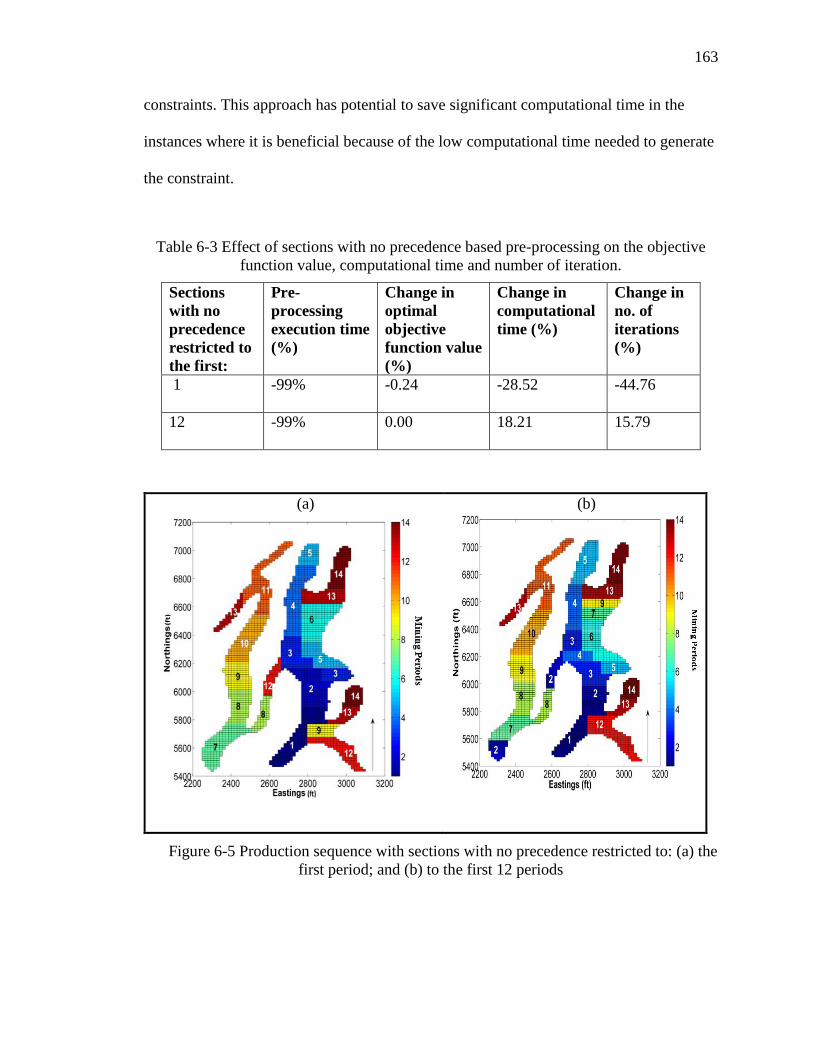
163

constraints. This approach has potential to save significant computational time in the

instances where it is beneficial because of the low computational time needed to generate

the constraint.

Table 6-3 Effect of sections with no precedence based pre-processing on the objective

function value, computational time and number of iteration.

Sections

with no

precedence

restricted to

the first:

Pre-

processing

execution time

(%)

Change in

optimal

objective

function value

(%)

Change in

computational

time (%)

Change in

no. of

iterations

(%)

1 -99% -0.24 -28.52 -44.76

12 -99% 0.00 18.21 15.79

(a)

(b)

Figure 6-5 Production sequence with sections with no precedence restricted to: (a) the

first period; and (b) to the first 12 periods

164

6.4.5.3. Based on sections in the development area. Table 6-4 shows the

change in objective function value, computational time, and number of iterations as well

as the pre-processing execution time for implementing the cutting plane based on sections

in the development area. Figure 6-6 shows the production sequence obtained when the

cutting planes based on sections in the development area was implemented as a pre-

processing technique to the BILP problem. The application of this techniques involved

evaluating two different scenarios. Similar to the previous techniques, a strict cutting

plane is implemented to reduce the feasible search space. The cutting plane was further

relaxed to evaluate the effect on the computational time, number of iteration and the

objective function value. In this case study, 12 sections (Figure 6-3) are found in the

development area. From the solution (Figure 5-6 (b)) in Chapter 5, it is optimal to mine

all 12 blocks before period 6.

In the first scenario, the development sections are restricted to the first 5 periods.

The sequence (Figure 6-6) obtained was optimal with significant decrease in the

computational time and the number of iterations. The computational time and the number

of iterations decreased by 22.95 % and 17.24 %, respectively.

In the second scenario, the cutting plane was relaxed to evaluate the effect on the

complexity of the problem. The sections in the development area were restricted to be

mined in the first 12 periods. Although the solution obtained (Figure 6-6) was optimal,

pre-processing the problem with the cutting plane did not improve the computational time

or the number of iterations. In fact, the number of iterations increased by as much as

76.48 % with a 37.55 % increase in the computational time.

165

The pre-processing execution time of the algorithm alone was 3.72% higher

(25.79 seconds), given that CPLEX can solve the problem in 24.83 seconds without any

pre-processing.

Table 6-4 Effect of sections in development area based pre-processing on the

computational complexity of the problem.

Sections in the

development

area

restricted to

the first:

Pre-

processing

execution time

(%)

Change in

optimal

objective

function value

(%)

Change in

computational

time (%)

Change in

no. of

iterations

(%)

5 3.72 0.00 -22.95 -17.24

12 3.72 0.00 37.55 76.48

Figure 6-6 Production sequence based on pre-processing with development sections

166

6.4.5.4. General discussions. Of the three pre-processing techniques evaluated,

the cutting plane generated based on sections in the development area resulted in optimal

solutions in both scenarios. An optimal solution was obtained by implementing the

greedy algorithm with very little restrictions on the search space. To minimize

computational time needed to solve the BILP problem, the best pre-processing approach

is the implementation of the cutting plane based on development sections. The pre-

processing algorithm must be significantly improved to fully benefit from the

development sections based approach.

From these results, it appears the effectiveness of cutting planes used to pre-

process production sequencing problems depends on the characteristics of the problem.

For the case study evaluated, the precedence constraints imposed by the primary

development drive the solution (see Section 5.4.2). From Table 5-2 it can be seen that the

problem is heavily constrained. The effect of the precedence constraint can be seen in the

optimal solution as well. Therefore, a pre-processing technique based on the development

sections is the best approach for the problem. Further experiments are necessary to

determine whether development based pre-processing cutting planes will be superior for

all types of R&P mine sequencing problems.

The objective of this research was to test the hypothesis that heuristic pre-

processing can be used to improve the computational efficiency of the branch and cut

solution to the R&P BILP problem. The sections in development area and greedy

algorithm-based cutting planes resulted in significantly less computational time and

number of iterations. The execution time, however, exceeded the computational time

prior to pre-processing, resulting in a higher computational time overall. Based on the

167

BILP R&P problem characteristics, the sections in development area-based cutting plane

is likely to improve the computational efficiency of the branch and cut solution. The

execution time of the sections in development based-cutting plane, however, exceeds the

computational time saved after pre-processing. A more efficient algorithm is needed to

generate valid cutting planes in order to appreciate the full benefit of the pre-processing

approach. There is, therefore, no substantial evidence that heuristic pre-processing can

improve the computational efficiency of branch and cut solutions. Further work is

necessary to determine whether the results obtained in this analysis can be extended to

other instances of this problem.

Although the overall pre-processing execution time for the sections with no

precedence-based cutting planes was significantly small, it did not improve the

computation efficiency for the R&P BILP problem. If the problem was such that, it is

optimal to mine sections with no precedence in the defined periods, the application of this

pre-processing approach could potentially improve the branch and cut solution. Further

work is needed to investigate the optimal conditions under which the sections with no

precedence pre-processing approach will be beneficial.

6.5. SUMMARY

In this chapter, the effect of pre-processing techniques on the computational

efficiency (computational time and number of iteration) of a production sequencing

problem is evaluated. Three techniques were used to generate problem specific cutting

planes to reduce the feasible search space before solving with the branch and cut

algorithm. Three cutting planes were developed and analyzed using the simulated R&P

lead mine sequencing problem developed in Chapter 5. The cutting planes were

developed based on: (1) on the greedy algorithm; (2) sections with no precedence

168

constraints; and (3) sections in the development area. The objective was to test the

hypothesis that heuristic pre-processing can be used to increase the computational

efficiency of branch and cut solutions to the BILP problem of R&P mine scheduling.

Based on the results obtained in the experiments here, this author concludes there

is not enough evidence to determine whether heuristic pre-processing increases the

computational efficiency of branch and cut solutions or not. Although some of the cutting

planes evaluated resulted in optimal solutions with less computational time and fewer

number of iterations, the computational time required to generate these cutting planes

was very high. This resulted in higher computational time overall. The one cutting plane

algorithm with very little computational time did not perform well (with respect to

number of iterations or computational time for the branch and cut algorithm). At this

time, it is not clear whether these observations can be extended to all instances of the

R&P BILP problem.

The solution indicates that implementing a cutting plane based on the sections in

the development area significantly reduces the number of iterations and solution time

needed to solve the problem. This is most likely because of the nature of the problem,

which is highly constrained with solutions controlled significantly by precedence

constraints of the primary development. The optimal solution was driven by the

precedence constraints instead of the section values. Therefore, pre-processing with the

greedy algorithm based cutting planes did not reduce the complexity of the problem

significantly. By relaxing the greedy algorithm based constraints, the search space

included the solutions that mine the development blocks in earlier periods as constrained

169

by precedence. This resulted in an optimal solution. Implementing the cutting plane based

on sections with no precedence constraint, however, did not result in an optimal solution.

The changes in computational time and number of iterations depends on the

nature and size of the problem, and the restrictions imposed by the cutting plane. Future

work must include developing a more efficient algorithm for generating the sections in

development area-based cutting planes. It is also necessary to determine whether the

results obtained can be extended to other instances of the R&P BILP problem. Further

investigation is needed to determine the optimum conditions under which the section with

no precedence pre-processing approach will be beneficial. As part of the cutting plane

pre-processing method, an algorithm should be developed that evaluates the validity of

each cutting plane generated prior to pre-processing. A valid cutting plane reduces the

feasible search space without eliminating the optimal solution. The effect of pre-

processing a real-life problem with cutting planes on computational time and the number

of iterations should be evaluated as well.

170

7. CONCLUSIONS AND RECOMMENDATIONS FOR FUTURE WORK

7.1. SUMMARY

A key part of mine planning is the need to optimize the production system.

Historically, engineers have used various tools to optimize mine plans and designs. The

pioneering approaches were trial and error methods. However, the complex nature of

mining systems makes trial and error methods sub-optimal in maximizing the value of the

mine. The continuous improvement of computational power and technology has made

more techniques available that enable engineers to model complex systems and analyze

different alternatives. One such technique is operations research and management science

(ORMS), which is the single most prominent method used to optimize systems today.

The choice of mine design parameters affects the way mines are run through all

stages of a mine. The sequence in which blocks are extracted significantly affects the

value of the mine. Based on current technology and economic conditions, a mining

sequence can be optimized to meet production and quality targets in each period.

Due to the ever challenging operating and market conditions, mining methods

such room and pillar used to mine coal resources must be optimized to minimize the unit

cost of production. Design parameters such as panel width affect the recovery,

productivity, unit cost, and haulage efficiency of the operation. The dimensions of the

panel affects the production (cut) sequence with larger panels resulting in more complex

cut sequencing and tramming by the CM and smaller panels resulting in equipment

congestion. It is therefore essential that dimensions of the coal panel are optimized.

Although production sequencing in R&P mines is essential, the uniformity of

most coal deposit makes the extraction sequence less complex. On the other hand, the

erratic nature of metal deposits makes sequencing in R&P metal mines a challenge.

171

Production sequencing in R&P pillar mining must account for risk (such as geological,

production and market risk) associated with material extraction.

The goal of this research was to use operations research techniques to model,

evaluate and select optimal alternatives to some critical R&P mine design parameters as

well as mine production sequences. In accordance with the overall goal of this research

the specific objectives are:

1. Apply discrete event simulation (DES) to determine the optimal width of

coal R&P panels under specific mining conditions;

2. Investigate whether the shuttle car fleet size used to mine a particular

panel width is optimal in different segments of the panel;

3. Test the hypothesis that binary integer linear programming (BILP) can be

used to account for mining risk in R&P long range mine production

sequencing; and

4. Test the hypothesis that heuristic pre-processing can be used to increase

the computational efficiency of branch and cut solutions to the BILP

problem of R&P mine sequencing.

The first two objectives apply to coal R&P mines. A discrete event simulation of

an existing coal R&P mine, capable of evaluating the effect of varying optimal panel

width on productivity and cost, was built using Arena ® simulation software. The

developed simulator was also used to study whether the shuttle car fleet size used to mine

a particular panel width is optimal in different segments of the panel.

The last two objectives apply to metal R&P mines. To achieve the third objective,

a binary integer linear program was developed that maximizes the overall net present

172

value of the operation while minimizing multiple risks. The model was subject to

resource, mining rate, quality, reserve, and precedence constraints. The BILP model was

coded in Matlab® and solved using ILOG CPLEX® solver through the CPLEX API for

Matlab®. The fourth objective examines the effect of pre-processing techniques based on

the problem’s characteristics on the computational time and number of iterations needed

to solve the problem. The pre-processing techniques involved developing specialized

cutting planes that minimizes the feasible search space before solving the problem with

CPLEX®. The pre-processing techniques are demonstrated using the simulated BILP

problem.

7.2. CONCLUSIONS

Based on the work done in this dissertation several conclusions can be drawn:

1. With respect to the first objective (coal R&P panel width optimization):

a. The research shows it is possible to use a DES approach to determine

the optimal panel width. A valid DES model has been built and

successfully used to determine the optimal width for an operating

mine.

b. For the mining system evaluated, increasing the number of entries

(panel width) increases the total production and the duration of

mining. It can also be concluded that a smaller panel width for initial

advance outperforms a larger panel width. Specifically, it is optimal

for the mine to use an 11-entry initial advance rather than a 13-entry

one. For a given number of shuttle cars, there appear to be an optimal

panel width that optimizes productivity.

173

c. The unit cost of mining decreased as the panel width was increased.

This was due to the fact that the fixed cost significantly outweighed

the variable cost (Equation (3-3)). Based on productivity alone, a 17-

entry panel was observed to be the optimal panel width for the existing

system which operates with four cars per CM.

d. Sensitivity analysis of unit cost and productivity to changing shuttle

car fleet size showed that, the productivity and unit cost increases as

the number of cars were increased. However, the change in unit cost

due to an additional shuttle car outweighs the changes in productivity.

The optimal number of entries that maximizes productivity changes as

the number of shuttle cars changes. Based on the results, a fleet size of

four was deemed to be optimal for mining the entire panel.

2. With respect to the second objective (the effect of changing duty cycles on

CM-Shuttle car matching):

a. This research successfully promulgated a DES-based approach for

accounting for changing duty cycles in optimal CM-shuttle car

matching. The proposed approach includes criteria used to define

segments that reflect changing equipment cycle times.

b. From the case study, it can be concluded that the fleet size used to

mine a particular panel width was not always optimal for all segments

of the panel. Any analysis that ignores the varying duty cycles in

different segments of a panel (such as the analysis in Chapter 3) is

174

likely to overestimate the optimal number of shuttle cars needed to

meet production demands.

c. For the panel width evaluated, it was found that three out of the 14

panel segments can attain a maximum productivity level using a three

shuttle cars per CM instead of four. Using three shuttle cars per CM to

mine these segments saves the mine $5,862 per panel.

3. With respect to the third objective (accounting for risk in R&P production

sequencing models):

a. The research demonstrates that a deterministic binary integer linear

programming approach can be used to model and incorporate multiple

mining risks in R&P production sequence optimization.

b. The significance of risk in production sequencing can be controlled by

introducing effective ratios. Verification with a simulated lead room

and pillar production sequencing problem indicates that changing the

importance of mining risk in production sequencing can significantly

change the optimal sequence.

c. The use of a block aggregation technique minimized the number of

constraints in the BILP problem. For the problem evaluated the

computational time reduced four fold when the blocks were

aggregated. Further experiments showed that this gain is true (if not as

pronounced) even when the optimization problem has less complicated

precedence constraints.

175

d. The aggregation of geologic blocks into sections and the elimination of

block precedence constraint for the problem minimizes mining

selectivity and, thus, affects the optimal value.

4. With respect to the fourth objective (investigating the effect of pre-processing

on the computational efficiency of production sequencing problems):

a. Implementing a cutting plane based on the sections in the development

area significantly reduces the number of iterations and solution time

needed to solve the problem. This is most likely because of the nature

of the problem, which is highly constrained with solutions controlled

significantly by precedence constraints of the primary development.

Pre-processing with the greedy algorithm based cutting planes did not

reduce the complexity of the problem significantly. Implementing the

cutting plane based on sections with no precedence constraint,

however, did not result in an optimal solution.

b. There is not enough evidence (based on the analysis in this work) to

determine whether heuristic pre-processing increases the

computational efficiency of branch and cut solutions or not. Some of

the cutting planes developed in this research resulted in optimal

solutions with less computational time and less number of iterations.

However, the computational time required to generate these cutting

planes were very high resulting in higher computational time overall.

c. The most promising cutting plane algorithm is the cutting plane based

on blocks with no precedence constraint. This algorithm required very

176

little computational time and could therefore result in lower solution

times, overall. However, the cutting plane did not perform well (with

respect to number of iterations or computational time for the branch

and cut algorithm) in the experiments in this work.

7.3. CONTRIBUTION OF THE PHD RESEARCH

1. This research was the first attempt to optimize productivity and unit mining

cost as a function of coal panel width. The implicit nature of the objective

function makes it difficult to use analytical tools to solve the problem. This

challenge was overcome by modeling the mining system as a stochastic

discrete event-based simulation capable of evaluating alternative panel width.

2. This research extends the work on accounting for changing duty cycles in fleet

size optimization to a R&P mining system. A novel frame work on how to

discretize the system into reasonable periods of operation (segments) to

facilitate realistic solutions was introduced. The approach balances the need to

optimize for changing duty cycles with realistic and reasonable operating

periods. The case study shows that this approach is viable and when used

properly can lead to savings in production costs.

3. An experimental approach was introduced that investigates the sensitivity of

productivity, cycle times, utilization, and duration of mining to changing duty

cycle with minimum computational effort. This is a contribution to simulation

methods as a novel simulation experiment design approach.

4. This work makes a contribution to the research on how to account for risk in

mine production sequencing models. A novel deterministic framework was

177

presented that models multiple mining risks using a binary integer linear

programming framework.

5. This work confirms that aggregation methods, used properly, can reduce the

computational time and number of iterations required to solve mine

production sequencing problem. This work, more than any that the author is

aware of, presents a systematic evaluation of this result with respect to the

complexity of the precedence constraints.

6. This work is the first attempt to investigate the effect of pre-processing

techniques, based on multiple specialized cutting planes, on the number of

iterations and computational time of a R&P production sequencing problem.

7. The research has proposed algorithms for three specialized cutting planes

which can be used as pre-processing techniques prior to solving with branch

and cut algorithms.

7.4. RECOMMENDATIONS FOR FUTURE WORK

The following recommendations for future work could improve and add to the

body of knowledge from this research:

1. Optimization methods for other important design parameters that affect

unit mining cost and productivity in coal panels:

In order to further improve the efficiency of mining operations in coal

R&P mines, researchers have to develop optimization methods for other

important design parameters such as those associated with conveyor belt, roof

support, panel, roof span, panel pillars, haul routes, and barrier pillars. The

parameters often optimized in room and pillar mines are those related to

geotechnical properties of the ore and hanging wall. Other factors that affect

178

the productivity and unit cost are rarely optimized. R&P mines have lower

production levels compared to longwall and surface coal mines. To improve

the efficiency of this mining method, all mine design parameters should be

optimized to increase productivity and minimize unit mining cost.

2. Optimizing coal recovery as a function of panel dimensions:

In this research, the panel width was optimized with regards to the unit

cost and productivity. The dimension of the panel significantly affects the coal

recovery as it affects the number and size of barrier pillars. Also, the

orientation and the size of a panel will affect the overall amount of coal

recovered from the mine. It is therefore essential to optimize coal recovery as

a function of panel dimensions as well.

3. Accounting for input correlation in fleet size optimization:

In this study, the input data was assumed to be independently and

identically distributed. In most operations correlation exists between mine

parameters (Que et al. 2015). Disregarding correlation when it exists may

result in under/over estimating the number of haulage equipment needed to

maximize productivity. Future work should evaluate whether correlation

exists between the various input variables and determine how to account for

any correlation in the model.

4. Accounting for pillar extraction in R&P production sequencing:

Although the model in this research included variables that represent

the extraction of pillars, the effect of pillar extraction on the mining sequence

was not evaluated. The model can be used to analyze the impact of pillar

179

extraction as an integral part of long range planning on the overall net present

value of the mine.

5. Comprehensive study of the computational complexity of the BILP R&P

mine sequencing problem:

Further work is required to evaluate other factors that affect the

computational complexity (solution time and number of iterations) of the

BILP R&P mine sequencing problem. For example, the effect of the number

of decision variables (number of blocks and sections) on the computational

time needs to be evaluated with carefully defined test problems. The effect of

sections (or block aggregation) should be examined and optimal aggregation

strategies recommended as well. Also, research is necessary to explore what

specific instances of the problem are more difficult to solve than others.

6. Evaluating problem specific cutting plane-based pre-processing

techniques:

The research evaluated three cutting plane-based pre-processing

techniques. Other pre-processing techniques can be developed and tested

based on the characteristics of the problem. Also, further work is required to

test the effectiveness of the three techniques developed and any additional

techniques using well designed test problems. The goal will be to demonstrate

the conditions under which a particular cutting plane will be effective in

reducing the computational time and number of iterations.

7. Developing tests to evaluate the validity of pre-processing cutting planes:

180

The research did not develop an efficient algorithm for testing the

validity of a cutting plane. The only test used in this research was solving the

LP relaxation of the problem with the cutting plane to see if it is feasible or

not. The results from the application of the greedy algorithm and sections with

no precedence based cutting planes, showed that the optimal solution was

eliminated from the feasible space. This showed that the test was inadequate

(i.e. the LP relaxation could be feasible but still eliminate the global optimal).

Using a trial and error approach to determine the validity of the cutting plane

will be time consuming and may not address the issue. Further work must be

done as part of the development of pre-processing algorithms to validate the

specialized cutting planes generated.

181

APPENDIX A.

ARENA DES MODEL AND HAULAGE

DISTANCES

182

APPENDIX A: PANEL WIDTH OPTIMIZATION

Arena DES model

183

Haul distances for the left-hand-side of the panel based on the 11 entries cut sequence in Figure 3-8(a).

Cut Number Cut Entry Outgoing Direction Distance (ft)

To Feeder From Feeder Total

1 4 2 down, 1 right, 1 down, 1 right 338 458 796

2 3 2 down, 2 right, 1 down, 1 right 398 518 916

3 5 3 down, 1 right 278 398 676

4 4 2.5 down, 1 right, 1 down, 1 right 368 488 856

5 3 2.5 down, 2 right, 1 down, 1 right 428 548 976

6 6 2 down, 1 left, 1 down, 1 right 338 338 676

7 5 3.5 down, 1 right 308 428 736

8 between 4 & 5 turn 3 down, 1 right, 1 down, 1 right 398 518 916

9 between 3 & 4 turn 3 down, 2 right, 1 down, 1 right 458 578 1036

10 2 2 down, 3 right, 1 down, 1 right 458 458 916

11 6 2.5 down, 1 left, 1 down, 1 right 368 368 736

12 between 4 & 5 hole 3.5 down, 1 right, 1 down, 1 right 428 548 976

13 4 3.5 down, 1 right, 1 down, 1 right 428 548 976

14 between 3 & 4 hole 3.5 down, 2 right, 1 down, 1 right 488 608 1096

15 3 3.5 down, 2 right, 1 down, 1 right 488 608 1096

16 2 2.5 down, 3 right, 1 down, 1 right 488 488 976

184

Haul distances for the left-hand-side of the panel based on the 11 entries cut sequence in Figure 3-8(a). Cont.

Cut Number Cut Entry Outgoing Direction Distance (ft)

To Feeder From Feeder Total

17 1 2 down, 4 right, 1 down, 1 right 518 518 1036

18 5 4 down, 1 right 338 458 796

19 between 5 & 6 1 left, 3 down, 1 right, 1 down, 1 right 458 458 916

20 4 4 down, 1 right, 1 down, 1 right 458 578 1036

21 3 4 down, 2 right, 1 down, 1 right 518 638 1156

22 between 3 & 2 1 right, 3 down, 1 right, 1 down, 1 right 458 458 916

23 1 2.5 down, 4 right, 1 down, 1 right 548 548 1096

24 6 3 down, 1 left, 1 down, 1 right 398 398 796

25 5 5 down, 1 right 398 518 916

26 between 4 & 5 turn 4 down, 1 right, 1 down, 1 right 458 578 1036

27 between 3 & 4 turn 4 down, 2 right, 1 down, 1 right 518 638 1156

28 2 3.5 down, 3 right, 1 down, 1 right 548 548 1096

29 between 2 & 1 1 right, 3 down, 2 right, 1 down, 1 right 518 518 1036

30 6 4 down, 1 left, 1 down, 1 right 458 458 916

31 between 4 & 5 hole 4.5 down, 1 right, 1 down, 1 right 488 608 1096

32 4 4.5 down, 1 right, 1 down, 1 right 488 608 1096

33 between 3 & 4 hole 4.5 down, 2 right, 1 down, 1 right 548 668 1216

185

Haul distances for the left-hand-side of the panel based on the 11 entries cut sequence in Figure 3-8(a). Cont.

Cut Number Cut Entry Outgoing Direction Distance (ft)

To Feeder From Feeder Total

34 3 4.5 down, 2 right, 1 down, 1 right 548 668 1216

35 2 4 down, 3 right, 1 down, 1 right 578 578 1156

36 1 3.5 down, 4 right, 1 down, 1 right 608 608 1216

37 6 4.5 down, 1 left, 1 down, 1 right 488 488 976

38 5 5.5 down, 1 right 428 548 976

39 between 4 & 5 turn 5 down, 1 right, 1 down, 1 right 518 638 1156

40 between 3 & 4 turn 5 down, 2 right, 1 down, 1 right 578 698 1276

41 between 3 & 2 1 right, 4 down, 1 right, 1 down, 1 right 518 518 1036

42 1 4 down, 4 right, 1 down, 1 right 638 638 1276

43 between 4 & 5 hole 5.5 down, 1 right, 1 down, 1 right 548 668 1216

44 between 3 & 4 hole 5.5 down, 2 right, 1 down, 1 right 608 728 1336

45 2 4.5 down, 3 right, 1 down, 1 right 608 608 1216

46 between 2 & 1 1 right, 4 down, 2 right, 1 down, 1 right 578 578 1156

47 between 5 & 6 1 left, 5 down, 1 right, 1 down, 1 right 578 578 1156

48 between 3 & 2 1 right, 5 down, 1 right, 1 down, 1 right 578 578 1156

49 1 4.5 down, 4 right, 1 down, 1 right 668 668 1336

50 between 2 & 1 1 right, 5 down, 2 right, 1 down, 1 right 638 638 1276

186

Haul distances for the right-hand-side of the panel based on the 11 entries cut sequence in Figure 3-8 (a). Cont.

Cut Number Cut Entry Outgoing Direction Distance (ft)

To Feeder From Feeder Total

1 8 2 down, 1 left, 1 down, 1 left 338 458 796

2 9 2 down, 2 left, 1 down, 1 left 398 518 916

3 7 3 down, 1 left 278 398 676

4 8 2.5 down, 1 left, 1 down, 1 left 368 488 856

5 9 2.5 down, 2 left, 1 down, 1 left 428 548 976

6 7 3.5 down, 1 left 308 428 736

7 between 8 & 7 turn 3 down, 1 left, 1 down, 1 left 398 518 916

8 between 9 & 8 turn 3 down, 2 left, 1 down, 1 left 458 578 1036

9 10 2 down, 3 left, 1 down, 1 left 458 458 916

10 11 2 down, 4 left, 1 down, 1 left 518 518 1036

11 between 8 & 7 hole 3.5 down, 1 left, 1 down, 1 left 428 548 976

12 8 3.5 down, 1 left, 1 down, 1 left 428 548 976

13 between 9 & 8 hole 3.5 down, 2 left, 1 down, 1 left 488 608 1096

14 9 3.5 down, 2 left, 1 down, 1 left 488 608 1096

15 10 2.5 down, 3 left, 1 down, 1 left 488 488 976

16 11 2.5 down, 4 left, 1 down, 1 left 548 548 1096

17 7 4.5 down, 1 left 368 488 856

187

Haul distances for the right-hand-side of the panel based on the 11 entries cut sequence in Figure 3-8 (a). Cont.

Cut Number Cut Entry Outgoing Direction Distance (ft)

To Feeder From Feeder Total

18 between 7 & 6 1 right, 3 down, 1 left, 1 down, 1 left 458 458 916

19 8 4 down, 1 left, 1 down, 1 left 458 578 1036

20 9 4 down, 2 left, 1 down, 1 left 518 638 1156

21 between 9 & 10 1 left, 3 down, 1 left, 1 down, 1 left 458 458 916

22 7 5 down, 1 left, 398 518 916

23 between 8 & 7 turn 4 down, 1 left, 1 down, 1 left 458 578 1036

24 between 9 & 8 turn 4 down, 2 left, 1 down, 1 left 518 638 1156

25 10 3.5 down, 3 left, 1 down, 1 left 548 548 1096

26 between 10 & 11 1 left, 3 down, 2 left, 1 down, 1 left 518 518 1036

27 between 8 & 7 hole 4.5 down, 1 left, 1 down, 1 left 488 608 1096

28 8 4.5 down, 1 left, 1 down, 1 left 488 608 1096

29 between 9 & 8 hole 4.5 down, 2 left, 1 down, 1 left 548 668 1216

30 9 4.5 down, 2 left, 1 down, 1 left 548 668 1216

31 10 4 down, 3 left, 1 down, 1 left 578 578 1156

32 11 3.5 down, 4 left, 1 down, 1 left 608 608 1216

33 7 5.5 down, 1 left 428 548 976

34 between 7 & 6 1 right, 4 down, 1 left, 1 down, 1 left 518 518 1036

188

Haul distances for the right-hand-side of the panel based on the 11 entries cut sequence in Figure 3-8 (a). Cont.

Cut Number Cut Entry Outgoing Direction Distance (ft)

To Feeder From Feeder Total

35 between 8 & 7 turn 5 down, 1 left, 1 down, 1 left 518 638 1156

36 between 9 & 8 turn 5 down, 2 left, 1 down, 1 left 578 698 1276

37 between 9 & 10 1 left, 4 down, 1 left, 1 down, 1 left 518 518 1036

38 11 4 down, 4 left, 1 down, 1 left 638 638 1276

39 between 6 & 5 1 right, 5 down, 1 left 458 458 916

40 between 8 & 7 hole 5.5 down, 1 left, 1 down, 1 left 548 668 1216

41 between 9 & 8 hole 5.5 down, 2 left, 1 down, 1 left 608 728 1336

42 10 4.5 down, 3 left, 1 down, 1 left 608 608 1216

43 between 10 & 11 1 left, 4 down, 2 left, 1 down, 1 left 578 578 1156

44 between 7 & 6 1 right, 5 down, 1 left, 1 down, 1 left 578 578 1156

45 between 9 & 10 1 left, 5 down, 1 left, 1 down, 1 left 578 578 1156

46 11 4.5 down, 4 left, 1 down, 1 left 668 668 1336

47 between 10 & 11 1 left, 5 down, 2 left, 1 down, 1 left 638 638 1276

50 between 2 & 1 1 right, 5 down, 2 right, 1 down, 1 right 638 638 1276

189

Haul distances for the left-hand-side of the panel based on the 13 entries cut sequence in Figure 3-8(b)

Cut

Number

Cut Entry Outgoing Direction Segments

to Feeder

Segments

from

Feeder

Distance (ft)

l

To Feeder From Feeder Total

1 4 2 down, 2 right, 1 down, 1 right 6 8 398 518 916

2 3 2 down, 3 right, 1 down, 1 right 7 9 458 578 1036

3 5 2 down, 1 right, 1 down, 1 right 5 7 338 458 796

4 4 2.5 down, 2 right, 1 down, 1 right 6.5 8.5 428 548 976

5 3 2.5 down, 3 right, 1 down, 1 right 7.5 9.5 488 608 1096

6 6 3 down, 1 right 4 6 278 398 676

7 5 2.5 down, 1 right, 1 down, 1 right 5.5 7.5 368 488 856

8 between 4 & 5 turn 3 down, 2 right, 1 down, 1 right 7 9 458 578 1036

9 between 3 & 4 turn 3 down, 3 right, 1 down, 1 right 8 10 518 638 1156

10 2 2 down, 4 right, 1 down, 1 right 8 8 518 518 1036

11 7 2 down, 1 left, 1 down, 1 right 5 5 338 338 676

12 6 4 down, 1 right 5 7 338 458 796

13 between 4 & 5 hole 3.5 down, 2 right, 1 down, 1 right 7.5 9.5 488 608 1096

14 4 3.5 down, 2 right, 1 down, 1 right 7.5 9.5 488 608 1096

190

Haul distances for the left-hand-side of the panel based on the 13 entries cut sequence in Figure 3-8(b). Cont.

Cut

Num

ber

Cut Entry Outgoing Direction Segments

to Feeder

Segments

from Feeder

Distance (ft)

l

To Feeder From Feeder Total

15 between 3 & 4

hole

3.5 down, 3 right, 1 down, 1 right 8.5 10.5 548 668 1216

16 3 3.5 down, 3 right, 1 down, 1 right 8.5 10.5 548 668 1216

17 2 2.5 down, 4 right, 1 down, 1 right 8.5 8.5 548 548 1096

18 1 2 down, 5 right, 1 down, 1 right 9 9 578 578 1156

19 7 3 down, 1 left, 1 down, 1 right 6 6 398 398 796

20 5 3.5 down, 1 right, 1 down, 1 right 6.5 8.5 428 548 976

21 between 5 & 6 1 left, 3 down, 2 right, 1 down, 1 right 8 8 518 518 1036

22 4 4 down, 2 right, 1 down, 1 right 8 10 518 638 1156

23 3 4 down, 3 right, 1 down, 1 right 9 11 578 698 1276

24 between 3 & 2 1 right, 3 down, 2 right, 1 down, 1 right 8 8 518 518 1036

25 1 2.5 down, 5 right, 1 down, 1 right 9.5 9.5 608 608 1216

26 6 4.5 down, 1 right 5.5 7.5 368 488 856

27 between 6 & 7 1 left, 3 down, 1 right, 1 down, 1 right 7 7 458 458 916

191

Haul distances for the left-hand-side of the panel based on the 13 entries cut sequence in Figure 3-8(b). Cont.

Cut

#

Cut Entry Outgoing Direction Segments

to Feeder

Segments

from Feeder

Distance (ft)

To Feeder From Feeder Total

28 5 4 down, 1 right, 1 down, 1 right 7 9 458 578 1036

29 between 4 & 5 turn 4 down, 2 right, 1 down, 1 right 8 10 518 638 1156

30 between 3 & 4 turn 4 down, 3 right, 1 down, 1 right 9 11 578 698 1276

31 2 3.5 down, 4 right, 1 down, 1 right 9.5 9.5 608 608 1216

32 between 2 & 1 1 right, 3 down, 3 right, 1 down, 1 right 9 9 578 578 1156

33 7 3.5 down, 1 left, 1 down, 1 right 6.5 6.5 428 428 856

34 6 5 down, 1 right 6 8 398 518 916

35 between 4 & 5 hole 4.5 down, 2 right, 1 down, 1 right 8.5 10.5 548 668 1216

36 4 4.5 down, 2 right, 1 down, 1 right 8.5 10.5 548 668 1216

37 between 3 & 4 hole 4.5 down, 3 right, 1 down, 1 right 9.5 11.5 608 728 1336

38 3 4.5 down, 3 right, 1 down, 1 right 9.5 11.5 608 728 1336

39 2 4 down, 4 right, 1 down, 1 right 10 10 638 638 1276

40 1 3.5 down, 5 right, 1 down, 1 right 10.5 10.5 668 668 1336

41 7 4 down, 1 left, 1 down, 1 right 7 7 458 458 916

42 5 4.5 down, 1 right, 1 down, 1 right 7.5 9.5 488 608 1096

192

Haul distances for the left-hand-side of the panel based on the 13 entries cut sequence in Figure 3-8(b). Cont.

Cut

#

Cut Entry Outgoing Direction Segments

to Feeder

Segments

from Feeder

Distance (ft)

To Feeder From Feeder Total

43 between 5 & 6 1 left, 4 down, 2 right, 1 down, 1 right 9 9 578 578 1156

44 between 4 & 5 turn 5 down, 2 right, 1 down, 1 right 9 11 578 698 1276

45 between 3 & 4 turn 5 down, 3 right, 1 down, 1 right 10 12 638 758 1396

46 between 3 & 2 1 right, 4 down, 2 right, 1 down, 1 right 9 9 578 578 1156

47 1 4 down, 5 right, 1 down, 1 right 11 11 698 698 1396

48 6 5.5 down, 1 right 6.5 8.5 428 548 976

49 between 4 & 5 hole 5.5 down, 2 right, 1 down, 1 right 9.5 11.5 608 728 1336

50 between 3 & 4 hole 5.5 down, 3 right, 1 down, 1 right 10.5 12.5 668 788 1456

51 2 4.5 down, 4 right, 1 down, 1 right 10.5 10.5 668 668 1336

52 between 2 & 1 2 right, 4 down, 2 right, 1 down, 1 right 10 10 638 638 1276

53 7 4.5 down, 1 left, 1 down, 1 right 7.5 7.5 488 488 976

54 between 5 & 6 1 left, 5 down, 2 right, 1 down, 1 right 10 10 638 638 1276

55 between 3 & 2 1 right, 5 down, 2 right, 1 down, 1 right 10 10 638 638 1276

56 1 4.5 down, 5 right, 1 down, 1 right 11.5 11.5 728 728 1456

193

Haul distances for the left-hand-side of the panel based on the 13 entries cut sequence in Figure 3-8(b). Cont.

57 between 6 & 7 1 left, 5 down, 1 right, 1 down, 1 right 9 9 578 578 1156

58 between 2 & 1 2 right, 5 down, 2 right, 1 down, 1 right 11 11 698 698 1396

Haul distances for the right-hand-side of the panel based on the 13 entries cut sequence in Figure 3-8(b).

Cut

Number

Cut Entry Outgoing Direction Segments to

Feeder

Segments from

Feeder

Distance (ft)

To Feeder From Feeder Total

1 10 2 down, 2 left, 1 down, 1 left 6 8 398 518 916

2 11 2 down, 3 left, 1 down, 1 left 7 9 458 578 1036

3 9 2 down 1 left, 1 down, 1 left 5 7 338 458 796

4 10 2.5 down, 2 left, 1 down, 1 left 6.5 8.5 428 548 976

5 11 2.5 down, 3 left, 1 down, 1 left 7.5 9.5 488 608 1096

6 8 3 down, 1 left 4 6 278 398 676

7 9 2.5 down, 1 left, 1 down, 1 left 5.5 7.5 368 488 856

8 between 10 & 9 turn 3 down, 2 left, 1 down, 1 left 7 9 458 578 1036

9 between 11 & 10 turn 3 down, 3 left, 1 down, 1 left 8 10 518 638 1156

10 12 2 down, 4 left, 1 down, 1 left 8 8 518 518 1036

194

Haul distances for the right-hand-side of the panel based on the 13 entries cut sequence in Figure 3-8(b). Cont.

Cut

Number

Cut Entry Outgoing Direction Segments

to Feeder

Segments

from

Feeder

Distance (ft)

To Feeder From

Feeder

Total

11 between 10 & 9 hole 3.5 down, 2 left, 1 down, 1 left 7.5 9.5 488 608 1096

12 10 3.5 down, 2 left, 1 down, 1 left 7.5 9.5 488 608 1096

13 between 11 & 10 hole 3.5 down, 3 left, 1 down, 1 left 8.5 10.5 548 668 1216

14 11 3.5 down, 3 left, 1 down, 1 left 8.5 10.5 548 668 1216

15 12 2.5 down, 4 left, 1 down, 1 left 8.5 8.5 548 548 1096

16 13 2 down, 5 left, 1 down, 1 left 9 9 578 578 1156

17 8 4 down, 1 left 5 7 338 458 796

18 9 3.5 down, 1 left, 1 down, 1 left 6.5 8.5 428 548 976

19 between 9 & 8 1 right, 3 down, 2 left, 1 down, 1 left 8 8 518 518 1036

20 10 4 down, 2 left, 1 down, 1 left 8 10 518 638 1156

21 11 4 down, 3 left, 1 down, 1 left 9 11 578 698 1276

22 between 11 & 12 1 left, 3 down, 2 left, 1 down, 1 left 8 8 518 518 1036

23 13 3 down, 5 left, 1 down, 1 left 10 10 638 638 1276

195

Haul distances for the right-hand-side of the panel based on the 13 entries cut sequence in Figure 3-8(b). Cont.

Cut # Cut Entry Outgoing Direction Segments

to Feeder

Segments

from

Feeder

Distance (ft)

24 8 4.5 down, 1 left 5.5 7.5 368 488 856

25 between 8 & 7 1 right, 3 down, 1 left, 1 down, 1 left 7 7 458 458 916

26 9 4 down, 1 left, 1 down, 1 left 7 9 458 578 1036

27 between 10 & 9 turn 4 down, 2 left, 1 down, 1 left 8 10 518 638 1156

28 between 11 & 10 turn 4 down, 3 left, 1 down, 1 left 9 11 578 698 1276

29 12 3.5 down, 4 left, 1 down, 1 left 9.5 9.5 608 608 1216

30 between 12 & 13 2 left, 3 down, 2 left, 1 down, 1 left 9 9 578 578 1156

31 between 10 & 9 hole 4.5 down, 2 left, 1 down, 1 left 8.5 10.5 548 668 1216

32 10 4.5 down, 2 left, 1 down, 1 left 8.5 10.5 548 668 1216

33 between 11 & 10 hole 4.5 down, 3 left, 1 down, 1 left 9.5 11.5 608 728 1336

34 11 4.5 down, 3 left, 1 down, 1 left 9.5 11.5 608 728 1336

35 12 4 down, 4 left, 1 down, 1 left 10 10 638 638 1276

36 13 3.5 down, 5 left, 1 down, 1 left 10.5 10.5 668 668 1336

37 8 5 down, 1 left 6 8 398 518 916

38 9 4.5 down, 1 left, 1 down, 1 left 7.5 9.5 488 608 1096

196

Haul distances for the right-hand-side of the panel based on the 13 entries cut sequence in Figure 3-8(b). Cont.

Cut

#

Cut Entry Outgoing Direction Segments

to Feeder

Segments

from Feeder

Distance

(ft)

To Feeder From Feeder Total

39 between 9 & 8 1 right, 4 down, 2 left, 1 down, 1 left 9 9 578 578 1156

40 between 10 & 9 turn 5 down, 2 left, 1 down, 1 left 9 11 578 698 1276

41 between 11 & 10 turn 5 down, 3 left, 1 down, 1 left 10 12 638 758 1396

42 between 11 & 12 1 left, 4 down, 2 left, 1 down, 1 left 9 9 578 578 1156

43 13 4 down, 5 left, 1 down, 1 left 11 11 698 698 1396

44 8 5.5 down, 1 left 6.5 8.5 428 548 976

45 between 8 & 7 1 right, 4 down, 1 left, 1 down, 1 left 8 8 518 518 1036

46 between 10 & 9 hole 5.5 down, 2 left, 1 down, 1 left 9.5 11.5 608 728 1336

47 between 11 & 10 hole 5.5 down, 3 left, 1 down, 1 left 10.5 12.5 668 788 1456

48 12 4.5 down, 4 left, 1 down, 1 left 10.5 10.5 668 668 1336

49 between 12 & 13 2 left, 4 down, 2 left, 1 down, 1 left 10 10 638 638 1276

50 between 7 & 6 1 right, 5 down, 1 left 7 7 458 458 916

51 between 9 & 8 1 right, 5 down, 2 left, 1 down, 1 left 10 10 638 638 1276

52 between 11 & 12 1 left, 5 down, 2 left, 1 down, 1 left 10 10 638 638 1276

197

Haul distances for the right-hand-side of the panel based on the 13 entries cut sequence in Figure 3-8(b). Cont.

Cut

#

Cut Entry Outgoing Direction Segments

to Feeder

Segments

from Feeder

Distance

(ft)

To Feeder From Feeder Total

53 13 4.5 down, 5 left, 1 down, 1 left 11.5 11.5 728 728 1456

54 between 8 & 7 1 right, 5 down, 1 left, 1 down, 1 left 9 9 578 578 1156

55 between 12 & 13 2 left, 5 down, 2 left, 1 down, 1 left 11 11 698 698 1396

Haul distances for the rooms in each section of the panel based on a 17 entries cut sequence (Figure 4-2).

Room Number or Location Cut no. in Room Outgoing Direction Distance (ft)

To Feeder From Feeder Total

Rm 3 2nd 2.5 left, 1 up, 3 left, 1 down, 1 left 548 548 1096

Rm 3 3rd 3.5 left, 1 up, 3 left, 1 down, 1 left 608 608 1216

Rm 3 4th 4 left, 1 up, 3 left, 1 down, 1 left 638 638 1276

Rm 3 5th 4.5 left, 1 up, 3 left, 1 down, 1 left 668 668 1336

Rm 3 6th 5.5 left, 1 up, 3 left, 1 down, 1 left 728 728 1456

Rm 4 1st 1 left, 2 up, 4 left, 1 down, 1 left 578 458 1036

198

Haul distances for the rooms in each section of the panel based on a 17 entries cut sequence (Figure 4-2). Cont.

Room Number or Location Cut no. in Room Outgoing Direction Distance (ft)

To Feeder From Feeder Total

Rm 4 2nd 1.5 left, 2 up, 4 left, 1 down, 1 left 608 488 1096

Rm 4 3rd 2.5 left, 2 up, 4 left, 1 down, 1 left 668 548 1216

Rm 4 4th 3 left, 2 up, 4 left, 1 down, 1 left 698 578 1276

Rm 4 5th 3.5 left, 2 up, 4 left, 1 down, 1 left 728 608 1336

Rm 4 6th 4.5 left, 2 up, 4 left, 1 down, 1 left 788 668 1456

Rm 5 1st 1 left, 3 up, 4 left, 1 down, 1 left 638 518 1156

Rm 5 2nd 1.5 left, 3 up, 4 left, 1 down, 1 left 668 548 1216

Rm 5 3rd 2.5 left, 3 up, 4 left, 1 down, 1 left 728 608 1336

Rm 5 4th 3 left, 3 up, 4 left, 1 down, 1 left 758 638 1396

Rm 5 5th 3.5 left, 3 up, 4 left, 1 down, 1 left 788 668 1456

Rm 5 6th 4.5 left, 3 up, 4 left, 1 down, 1 left 848 728 1576

Rm 6 1st 2 left, 4 up, 3 left, 1 down, 1 left 698 578 1276

Rm 6 2nd 2.5 left, 4 up, 3 left, 1 down, 1 left 728 608 1336

Rm 6 3rd 3.5 left, 4 up, 3 left, 1 down, 1 left 788 668 1456

Rm 6 4th 4 left, 4 up, 3 left, 1 down, 1 left 818 698 1516

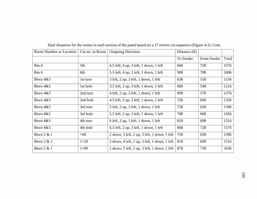
199

Haul distances for the rooms in each section of the panel based on a 17 entries cut sequence (Figure 4-2). Cont.

Room Number or Location Cut no. in Room Outgoing Direction Distance (ft)

To Feeder From Feeder Total

Rm 6 5th 4.5 left, 4 up, 3 left, 1 down, 1 left 848 728 1576

Rm 6 6th 5.5 left, 4 up, 3 left, 1 down, 1 left 908 788 1696

Btwn 4&3 1st turn 3 left, 2 up, 3 left, 1 down, 1 left 638 518 1156

Btwn 4&3 1st hole 3.5 left, 2 up, 3 left, 1 down, 1 left 668 548 1216

Btwn 4&3 2nd turn 4 left, 2 up, 3 left, 1 down, 1 left 698 578 1276

Btwn 4&3 2nd hole 4.5 left, 2 up, 3 left, 1 down, 1 left 728 608 1336

Btwn 4&3 3rd turn 5 left, 2 up, 3 left, 1 down, 1 left 758 638 1396

Btwn 4&3 3rd hole 5.5 left, 2 up, 3 left, 1 down, 1 left 788 668 1456

Btwn 4&3 4th turn 6 left, 2 up, 3 left, 1 down, 1 left 818 698 1516

Btwn 4&3 4th hole 6.5 left, 2 up, 3 left, 1 down, 1 left 848 728 1576

Btwn 2 & 1 +60 2 down, 3 left, 2 up, 3 left, 1 down, 1 left 758 638 1396

Btwn 2 & 1 1+20 2 down, 4 left, 2 up, 3 left, 1 down, 1 left 818 698 1516

Btwn 2 & 1 1+80 2 down, 5 left, 2 up, 3 left, 1 down, 1 left 878 758 1636

200

Haul distances for the rooms in each section of the panel based on a 17 entries cut sequence (Figure 4-2). Cont.

Room Number or Location Cut no. in Room Outgoing Direction Distance (ft)

To Feeder From Feeder Total

Btwn 2 & 1 2+40 2 down, 6 left, 2 up, 3 left, 1 down, 1 left 938 818 1756

Btwn 3 & 2 +60 1 down, 3 left, 2 up, 3 left, 1 down, 1 left 698 578 1276

Btwn 3 & 2 1+20 1 down, 4 left, 2 up, 3 left, 1 down, 1 left 758 638 1396

Btwn 3 & 2 1+80 1 down, 5 left, 2 up, 3 left, 1 down, 1 left 818 698 1516

Btwn 3 & 2 2+40 1 down, 6 left, 2 up, 3 left, 1 down, 1 left 878 758 1636

Btwn 4 & 5 +60 1 up, 1 left, 1 up, 5 left, 1 down, 1 left 638 518 1156

Btwn 4 & 5 1+20 1 up, 2 left, 1 up, 5 left, 1 down, 1 left 698 578 1276

Btwn 4 & 5 1+80 1 up, 3 left, 1 up, 5 left, 1 down, 1 left 758 638 1396

Btwn 4 & 5 2+40 1 up, 4 left, 1 up, 5 left, 1 down, 1 left 818 698 1516

Btwn 5 & 6 +60 3 up, 6 left, 1 down, 1 left 698 578 1276

Btwn 5 & 6 1+20 3 up, 7 left, 1 down, 1 left 758 638 1396

Btwn 5 & 6 1+80 3 up, 8 left, 1 down, 1 left 818 698 1516

Btwn 5 & 6 2+40 3 up, 9 left, 1 down, 1 left 878 758 1636

201

Haul distances for the rooms in each section of the panel based on a 17 entries cut sequence (Figure 4-2). Cont.

Room Number or Location Cut no. in Room Outgoing Direction Distance (ft)

To Feeder From Feeder Total

Btwn 6 & old +60 4 up, 6 left, 1 down, 1 left 758 638 1396

Btwn 6 & old 1+20 4 up, 7 left, 1 down, 1 left 818 698 1516

Btwn 6 & old 1+80 4 up, 8 left, 1 down, 1 left 878 758 1636

Btwn 6 & old 2+40 4 up, 9 left, 1 down, 1 left 938 818 1756

APPENDIX B.

CM-SHUTTLE CAR MATCHING EXPERIMENTAL

OUTPUT

203

APPENDIX B: CM-SHUTTLE CAR MATCHING EXPERIMENTAL OUTPUT

Duration of mining

Fleet size

Cuts Segment 1 2 3 4 5 6

Entries 1 15.84 10.37 9.04 9.01 8.98 8.87

Entries 2 17.34 11.19 9.58 9.49 9.40 9.34

Entries 3 17.38 11.24 9.59 9.21 9.14 9.10

Entries 4 18.61 11.76 9.75 9.39 9.34 9.31

Entries 5 17.68 11.33 9.64 9.34 9.32 9.25

Entries 6 16.70 10.99 9.44 9.23 9.25 9.09

Entries 7 17.13 11.16 9.53 9.47 9.43 9.30

Entries 8 18.00 11.61 9.75 9.26 9.24 9.17

Entries 9 18.93 11.93 9.84 9.48 9.47 9.45

Rooms 10 17.47 11.22 9.48 9.22 9.21 9.20

Rooms 11 18.02 11.56 9.58 9.17 9.13 8.96

Rooms 12 18.83 12.02 9.97 9.38 9.35 9.15

Rooms 13 18.98 12.05 10.00 9.32 9.32 9.18

Rooms 14 14.60 9.07 7.35 6.76 6.64 6.59

204

Cycle times LHS

Fleet size

Cuts Segment 1 2 3 4 5 6

Entries 1 4.15 5.42 7.07 9.37 11.65 13.78

Entries 2 4.54 5.85 7.50 9.88 12.18 14.48

Entries 3 4.55 5.87 7.48 9.55 11.83 14.09

Entries 4 4.87 6.15 7.63 9.79 12.15 14.51

Entries 5 4.63 5.92 7.54 9.74 12.13 14.44

Entries 6 4.37 5.73 7.37 9.59 11.97 14.04

Entries 7 4.48 5.82 7.43 9.82 12.19 14.39

Entries 8 4.71 6.06 7.63 9.61 11.95 14.15

Entries 9 4.96 6.22 7.70 9.87 12.32 14.71

Rooms 10 4.57 5.86 7.42 9.61 11.98 14.33

Rooms 11 4.72 6.04 7.50 9.56 11.89 13.95

Rooms 12 4.93 6.28 7.80 9.78 12.16 14.23

Rooms 13 4.97 6.29 7.80 9.71 12.09 14.26

Rooms 14 5.09 6.31 7.65 9.36 11.47 13.62

205

Cycle time RHS

Fleet size

Cuts Segment 1 2 3 4 5 6

Entries 1 4.27 5.56 7.21 9.57 11.86 14.00

Entries 2 4.62 5.94 7.63 10.16 12.53 14.92

Entries 3 4.82 6.21 7.85 9.97 12.28 14.67

Entries 4 4.93 6.19 7.66 9.78 12.13 14.47

Entries 5 4.47 5.73 7.34 9.62 11.98 14.24

Entries 6 4.62 6.05 7.65 9.96 12.40 14.65

Entries 7 4.73 6.12 7.76 10.25 12.71 15.05

Entries 8 4.83 6.23 7.85 9.99 12.38 14.72

Entries 9 4.71 5.93 7.40 9.57 11.96 14.26

Rooms 10 4.66 5.95 7.52 9.67 12.04 14.38

Rooms 11 4.79 6.14 7.59 9.58 11.95 14.03

Rooms 12 5.06 6.43 7.98 9.95 12.40 14.50

Rooms 13 5.20 6.57 8.13 9.90 12.30 14.53

Rooms 14 5.19 6.44 7.81 9.47 11.59 13.76

CM utilization for loading LHS

Fleet size

Cuts Segment 1 2 3 4 5 6

Entries 1 15.60 23.90 27.40 27.50 27.60 28.00

206

CM utilization for loading LHS. Cont.

Fleet size

Cuts Segment 1 2 3 4 5 6

Entries 2 14.30 22.10 25.90 26.10 26.30 26.50

Entries 3 14.20 22.00 25.80 26.90 27.10 27.20

Entries 4 13.30 21.10 25.40 26.40 26.60 26.60

Entries 5 14.00 21.90 25.70 26.50 26.60 26.80

Entries 6 14.80 22.50 26.20 26.80 26.70 27.20

Entries 7 14.50 22.20 26.00 26.10 26.30 26.60

Entries 8 13.70 21.30 25.40 26.70 26.80 27.00

Entries 9 13.10 20.80 25.20 26.10 26.10 26.20

Rooms 10 14.20 22.10 26.10 26.90 26.90 26.90

Rooms 11 13.70 21.40 25.80 27.20 27.20 27.70

Rooms 12 13.10 20.60 24.90 26.40 26.60 27.10

Rooms 13 13.00 20.60 24.80 26.60 26.70 27.10

Rooms 14 12.70 20.50 25.30 27.70 28.20 28.40

CM utilization for loading RHS

Fleet size

Cuts Segment 1 2 3 4 5 6

Entries 1 15.10 23.30 26.90 27.00 27.10 27.50

Entries 2 14.00 21.70 25.40 25.40 25.60 25.80

207

CM utilization for loading RHS. Cont.

Fleet size

Cuts Segment 1 2 3 4 5 6

Entries 3 13.40 20.70 24.60 25.80 26.10 26.10

Entries 4 13.10 20.90 25.30 26.40 26.60 26.70

Entries 5 14.50 22.50 26.30 26.80 26.90 27.10

Entries 6 14.00 21.30 25.20 25.80 25.80 26.10

Entries 7 13.70 21.00 24.80 26.10 25.10 25.40

Entries 8 13.40 20.70 24.60 25.70 25.80 25.90

Entries 9 13.70 21.80 26.10 26.90 26.90 27.00

Rooms 10 13.90 21.70 25.70 26.70 26.70 26.80

Rooms 11 13.50 21.00 25.50 27.00 27.00 27.60

Rooms 12 12.80 20.10 24.20 25.90 26.00 26.60

Rooms 13 12.40 19.60 23.80 26.10 26.10 26.50

Rooms 14 12.50 20.00 24.80 27.30 27.90 28.00

Average waiting time in loading queue LHS

Fleet size

Cuts Segment 1 2 3 4 5 6

Entries 1 1.48 1.97 2.54 3.18 3.75 4.31

Entries 2 1.73 2.29 3.00 3.89 4.57 5.37

Entries 3 1.76 2.33 2.98 3.46 4.01 4.75

208

Average waiting time in loading queue LHS. Cont.

Fleet size

Cuts Segment 1 2 3 4 5 6

Entries 4 1.89 2.37 2.78 3.36 3.88 4.42

Entries 5 1.78 2.29 2.89 3.42 4.08 4.69

Entries 6 1.67 2.30 2.91 3.56 4.32 4.99

Entries 7 1.73 2.33 2.98 3.80 4.53 5.17

Entries 8 1.87 2.49 3.15 3.62 4.25 4.91

Entries 9 1.91 2.40 2.89 3.47 4.09 4.54

Rooms 10 1.89 2.38 2.89 3.33 3.90 4.40

Rooms 11 1.96 2.55 3.06 3.46 4.09 4.46

Rooms 12 2.09 2.73 3.35 3.88 4.57 5.01

Rooms 13 2.05 2.65 3.26 3.64 4.20 4.69

Rooms 14 2.14 2.65 3.12 3.46 3.87 4.38

Average waiting time in loading queue RHS

Fleet size

Segment 1 2 3 4 5 6

1 1.48 1.88 2.37 2.91 3.46 3.92

2 1.71 2.13 2.65 3.36 3.88 4.38

3 1.86 2.44 2.94 3.24 3.67 4.19

4 1.88 2.31 2.75 3.20 3.76 4.30

209

Average waiting time in loading queue RHS. Cont.

Fleet size

Segment 1 2 3 4 5 6

5 1.63 2.06 2.56 3.02 3.54 3.97

6 1.79 2.38 2.87 3.42 4.09 4.67

7 1.78 2.31 2.81 3.53 4.16 4.70

8 1.86 2.38 2.90 3.41 3.93 4.48

9 1.82 2.23 2.68 3.24 3.81 4.46

10 1.88 2.31 2.82 3.40 4.00 4.68

11 1.95 2.42 2.73 3.14 3.54 3.87

12 2.07 2.60 3.09 3.35 3.82 4.06

13 2.15 2.66 3.08 3.29 3.79 4.11

14 2.14 2.47 2.69 2.96 3.18 3.36

Productivity

Fleet size

Cuts Tonnage in Segment Segment 1 2 3 4 5 6

Entries 5437 1 343 524 602 603 606 613

Entries 5158 2 297 461 538 543 549 552

Entries 4740 3 273 422 494 515 518 521

Entries 4182 4 225 356 429 445 448 449

Entries 5018 5 284 443 521 537 539 542

Entries 5158 6 309 469 546 559 558 567

210

Productivity. Cont.

Fleet size

Cuts Tonnage in Segment Segment 1 2 3 4 5 6

Entries 4740 7 277 425 497 501 502 509

Entries 4740 8 263 408 486 512 513 517

Entries 4529 9 239 380 460 478 478 479

Rooms 5403 10 309 482 570 586 587 587

Rooms 5117 11 284 443 534 558 560 571

Rooms 5117 12 272 426 513 546 547 559

Rooms 4971 13 262 412 497 533 534 542

Rooms 1754 14 120 193 239 260 264 266

211

BIBLIOGRAPHY

Achttien, D. B., and Stine, R. H. (1964). Computer simulation of a haulage system. In

Mining Congress Journal (pp. 41-46).

Akaike, A., and Dagdelen, K. (1999). A strategic production scheduling method for an

open pit mine. Proceedings of the 28th Application of Computers and Operation

Research in the Mineral Industry, 729-738.

Alarie, S., and Gamache, M. (2002). Overview of solution strategies used in truck

dispatching systems for open pit mines. International Journal of Surface Mining,

Reclamation and Environment, 16(1), 59-76.

Alford, C., Brazil, M., and Lee, D. H. (2007). Optimisation in underground mining. In

Handbook of operations research in natural resources (pp. 561-577). Springer US.

Almgren, T. (1994). An approach to long range production and development planning

with application to the Kiruna Mine, Doctorial thesis. Sweden.

Alonso-Ayuso, A., Carvallo, F., Escudero, L. F., Guignard, M., Pi, J., Puranmalka, R.,

and Weintraub, A. (2014). Medium range optimization of copper extraction planning

under uncertainty in future copper prices. European Journal of Operational Research,

233(3), 711-726.

Anani, A. and K. Awuah-Offei. (2013). Modeling room and pillar operation with pillar

retrieval as mixed integer linear programming. Proceedings of the Innovations in

Mining Engineering Conference, St. Louis, Missouri, September 9-12, 2013.

Anani, A. and K. Awuah-Offei. (2015). Modeling Mining Risk in Room and Pillar Mine

Sequencing Using Mixed Integer Linear Programming. Proceedings of the society for

mining metallurgy and exploration annual conference, Denver, Colorado, February

15-18, 2015.

Anastassiou, G. (Ed.). (2000). Handbook of Analytic Computational Methods in Applied

Mathematics. CRC Press.

Archambeault, L. (2007). Application of Artificial Intelligence to Mine Optimization and

Real Option Valuation. Australasian Institute of Mining and Metallurgy Publication

Series. 2007, Pages 159-168 Project Evaluation Conference 2007; Melbourne, VIC;

Australia; 19 June 2007 through 20 June 2007.

Askari-Nasab, H., Awuah-Offei, K., and Eivazy, H. (2010). Large-scale open pit

production scheduling using mixed integer linear programming. International Journal

of Mining and Mineral Engineering, 2(3), 185-214 .

Askari-Nasab, H., Pourrahimian, Y., Ben-Awuah, E., and Kalantari, S. (2011). Mixed

integer linear programming formulations for open pit production scheduling. Journal

of Mining Science, 47(3), 338-359.

212

Askari-Nasab, H., Torkamani, E., Badiozamani, M. M., and Tabesh, M. (2012).

Alignment of Short-Term and Operational Plans Using Discrete Event Simulation, in

Proceedings of Society for Mining, Metallurgy & Exploration (SME) Annual Meeting,

CD-ROM, Preprint 12-064, © SME, Seattle, Washington, USA, Feb. 19- 22, pp. 304-

311.

Asplund, S., and Jakobsson, T. (2011). Successful Discrete-Event Simulation Offshoring.

Master’s thesis. Chalmers university of Technology.

Ataeepour, N., and Baafi, E. Y. (1999). ARENA simulation model for truck-shovel

operation in despatching and non-despatching modes. International Journal of

Surface Mining, Reclamation and Environment, 13(3), 125-129.

Automation, R. (2012). Arena simulation software. Rockwell Automation, Version 14.

Awuah-Offei, K., Osei, B., and Askari-Nasab, H. (2012). Modeling Truck-Shovel Energy

Efficiency under Uncertainty, SME Transactions, Vol. 330, pp. 573-584.

Awuah-Offei, K., Temeng, V.A., and Al-Hassan, S. (2003). Predicting Equipment

Requirements Using SIMAN Simulation: A Case Study. Mining Technology, 112,

(3), 180-184.

Axelson A. H. (1964). A practical approach to computer utilization in mine planning

presented at the international symposium – applications of statistics, Operations

research and computers in the mineral industry, Colorado school of minies.

Baafi, E. Y., and Ataeepur, M. (1996). Simulation of a truck-shovel system using Arena.

In Proceeding of the 26th International Symposium on the Application of Computers

and Operations Research in the Mineral Industries (APCOM) (pp. 153-159).

Balas, E., Ceria, S., and Cornuéjols, G. (1993). A lift-and-project cutting plane algorithm

for mixed 0–1 programs. Mathematical programming, 58(1-3), 295-324.

Balas, E., Jeroslow, R. (1972). Canonical cuts on the unit hypercube. SIAM Journal of

Applied Mathematics, 23 (1), 61–69.

Balci, O. 1988. The implementation of four conceptual frameworks for simulation

modeling in high-level languages. In Proceedings of the 20th conference on Winter

simulation (pp. 287-295). ACM.

Banks, J. (Ed.). (1998). Handbook of simulation (pp. 3-389). New York: Wiley.

Barbaro, R. W., and Ramani, R. V. (1986). Generalized multiperiod MIP model for

production scheduling and processing facilities selection and location. Mining

Engineering, 38(2), 107-114.

Basu, A. J., and Baafi, E. Y. (1999). Discrete event simulation of mining systems: current

practice in Australia. International Journal of Surface Mining, Reclamation and

Environment, 13(2), 79-84.

Beamon, B. M., and Deshpande, A. N. (1998). A mathematical programming approach to

simultaneous unit-load and fleet-size optimisation in material handling systems

design. The international journal of advanced manufacturing technology, 14(11),

858-863.

213

Bellman, R. E. (1953). An introduction to the theory of dynamic programming, Rand

report.

Ben-Awuah, E., Kalantari, S., Pourrahimian, Y., and Askari-Nasab, H. (2010).

Hierarchical mine production scheduling using discrete-event simulation.

International Journal of Mining and Mineral Engineering, 2(2), 137-158.

Bienstock, D. and Zuckerberg, M. (2010). Solving LP Relaxations of Large-scale

Precedence Constrained Problems. Integer Programming and Combinatorial

Optimization, Eisenbrand, F. and Shepherd, F.B. (Eds.), Springer-Verlag Berlin

Heidelberg, 1-14.

Bienstock, D., and Zuckerberg, D. (2009). A new LP algorithm for precedence

constrained production scheduling. Optimization Online.

Bixby, R. E., and Lee, E. K. (1998). Solving a truck dispatching scheduling problem

using branch-and-cut. Operations Research, 46(3), 355-367.

Bley, A., Boland, N., Fricke, C., and Froyland, G. (2010). A strengthened formulation

and cutting planes for the open pit mine production scheduling problem. Computers

& Operations Research, 37(9), 1641-1647.

Boland, N., Dumitrescu, I., and Froyland, G. (2008). A multistage stochastic

programming approach to open pit mine production scheduling with uncertain

geology. Optimization Online.

Boland, N., Dumitrescu, I., Froyland, G., and Gleixner, A. M. (2009). LP-based

disaggregation approaches to solving the open pit mining production scheduling

problem with block processing selectivity. Computers & Operations Research, 36(4),

1064-1089.

Boyd, E. A. (1994). Fenchel cutting planes for integer programs. Operations Research,

42(1), 53-64.

Boyd, J., Bass, E. J., Patek, S. D., and Lee, D. W. (2006). Investigation of future air taxi

services using discrete-event simulation. In Systems and Information Engineering

Design Symposium, IEEE (pp. 25-30). IEEE.

Brickey, A. J. (2015). Underground Production Scheduling Optimization with Ventilation

Constraints, Doctoral dissertation, Colorado School of Mines.

Brunetta, L., Conforti, M., and Rinaldi, G. (1997). A branch-and-cut algorithm for the

equicut problem. Mathematical Programming, 78(2), 243-263.

Buchholz, P. (2009). Optimization of Stochastic Discrete Event Simulation Models. In

Dagstuhl Seminar Proceedings (pp. 1-5).

Burt, C., L. Caccetta, S. Hill, P. Welgama. (2005). Models for mining equipment

selection. A. Zerger, R. M. Argent, eds. MODSIM 2005, Internat. Congress

Modeling Simulation. Modelling and Simulation Society of Australia and New

Zealand, 1730–1736.

Buxton, J. N., and Laski, J. G. (1962). Control and simulation language. The Computer

Journal, 5(3), 194-199.

214

Caccetta, L., and Hill, S. P. (2003). An application of branch and cut to open pit mine

scheduling. Journal of global optimization, 27(2-3), 349-365.

Callow, D. J. (2006). The impact of mining conditions on mechanized mining

efficiency. Journal-South African Institute of Mining and Metallurgy, 106(12), 821.

Carmichael, D. G. (1986). Shovel–truck queues: a reconciliation of theory and practice.

Construction Management and Economics, 4(2), 161-177.

Carpentier, S., Gamache, M., and Dimitrakopoulos, R. (2015). Underground long-term

mine production scheduling with integrated geological risk management. Mining

Technology, 1743286315Y-0000000026.

Carson, Y., and Maria, A. (1997). Simulation optimization: methods and applications. In

Proceedings of the 29th conference on Winter simulation (pp. 118-126). IEEE

Computer Society.

Chakroborty, P., Deb, K., and Sharma, R. K. (2001). Optimal fleet size distribution and

scheduling of transit systems using genetic algorithms. Transportation Planning and

Technology, 24(3), 209-225.

Chen, C. H., Yücesan, E., Dai, L., and Chen, H. C. (2009). Optimal budget allocation for

discrete-event simulation experiments. IIE Transactions, 42(1), 60-70.

Chen, D. S., Batson, R. G., and Dang, Y. (2010). Applied integer programming:

modeling and solution. John Wiley & Sons.

Chen, M. U. (2009). Simulation study of cruising taxi operation system. Systems

Engineering-Theory & Practice, 11.

Chicoisne, R., Espinoza, D., Goycoolea, M., Moreno, E., and Rubio, E. (2012). A new

algorithm for the open-pit mine production scheduling problem. Operations

Research, 60(3), 517-528.

Chinneck, J. W. (2006). Practical optimization: a gentle introduction. Systems and

Computer Engineering, Carleton University, Ottawa. http://www. sce. carleton.

ca/faculty/chinneck/po. html.

Choobineh, F. F., Asef-Vaziri, A., and Huang, X. (2012). Fleet sizing of automated

guided vehicles: a linear programming approach based on closed queuing networks.

International Journal of Production Research, 50(12), 3222-3235.

Chugh Y.P, McGolden M, and Hirschi J. (2002). Identification of cost cutting strategies

for underground mines in Illinois. Final technical report (November 1, 2000, through

October 31, 2002). Office of coal development and marketing and the Illinois clean

coal institute.

Chung, C. A. (Ed.). (2003). Simulation modeling handbook: a practical approach. CRC

press.

Chvátal, V. (1973). Edmonds polytopes and a hierarchy of combinatorial problems.

Discrete mathematics, 4(4), 305-337.

Clausen, J. (1999). Branch and bound algorithms-principles and examples. Department of

Computer Science, University of Copenhagen, 1-30.

215

Coxeter, H. S. M. (1973). Regular polytopes. Courier Corporation.

Dagdelen, K., and Johnson, T. B. (1986). Optimum open pit mine production scheduling

by Lagrangian parameterization. In 19th APCOM Symposium of the society of mining

engineers (AIME).

Dahl, O. J., Myhrhaug, B., and Nygaard, K. (1967). Simula 67 common base language.

Dantzig, G. (1948). Programming in a linear structure. U.S. Air Force Comptroller,

USAF, Washington, D.C.

Darby-Dowman, K., and Rangel, S. (1998). The application of preprocessing and cutting

plane techniques for a class of production planning problems. Computational

Optimization and Applications, 11(3), 297-318.

Dimitrakopoulos, R. (1998). Conditional simulation algorithms for modelling orebody

uncertainty in open pit optimization. International Journal of Surface Mining,

Reclamation and Environment, 12(4), 173-179.

Dimitrakopoulos, R. (2004). Orebody uncertainty, risk assessment and profitability in

recoverable reserves, ore selection and mine planning, in conditional simulation

concepts and applications for the mining industry. In AusIMM-BRC 2004

Professional Development Seminar Series.

Dimitrakopoulos, R. (2011). Stochastic optimization for strategic mine planning: a

decade of developments. Journal of Mining Science, 47(2), 138-150.

Dimitrakopoulos, R., and Ramazan, S. (2004). Uncertainty based production scheduling

in open pit mining. SME transactions, 316.

Dindarloo, S. R., Osanloo, M., and Frimpong, S. (2015). A stochastic simulation

framework for truck and shovel selection and sizing in open pit mines. Journal of the

Southern African Institute of Mining and Metallurgy, 115(3), 209-219.

Dong, J. X., and Song, D. P. (2012). Quantifying the impact of inland transport times on

container fleet sizing in liner shipping services with uncertainties. OR spectrum,

34(1), 155-180.

Dowd, P.A. and Onur, A.H. (1993). Open pit optimisation: I - optimal open pit design.

Trans. Instn. Min. Metall., Section A, 102, A95-104.

Egbelu, P. J. (1987). The use of non-simulation approaches in estimating vehicle

requirements in an AGV based transport system, International Journal of Production

Research, 4, pp. 17-32, 1987.

Eglese, R. W. (1990). Simulated annealing: a tool for operational research. European

journal of operational research, 46(3), 271-281.

EIA .2014. Energy Information Administration Website. Department of Energy.

Eivazy, H., and Askari-Nasab, H. (2012). A hierarchical open-pit mine production

scheduling optimisation model. International Journal of Mining and Mineral

Engineering, 4(2), 89-115.

216

Ercelebi, S. G., and Bascetin, A. (2009). Optimization of shovel-truck system for surface

mining. Journal of The Southern African Institute of Mining and Metallurgy, 109,

433-439.

Fanti, M. P., Mangini, A. M., Pedroncelli, G., and Ukovich, W. (2014). Fleet sizing for

electric car sharing system via closed queueing networks. In Systems, Man and

Cybernetics (SMC), 2014 IEEE International Conference on (pp. 1324-1329), IEEE.

Farmer, I. (1992). Room-and-pillar Mining. SME Mining Engineering Handbook, 2nd

Ed., Hartman, H.L. (Ed.), Society for Mining, Metallurgy, and Exploration, Littleton,

CO, USA, Chapter 18, 1681-1701.

Fedorčáková, M., and Šebo, J. (2012). Innovative application of inventory theory for

determining optimal fleet size for a car-sharing system. In Applied Machine

Intelligence and Informatics (SAMI), 2012 IEEE 10th International Symposium on

(pp. 157-160), IEEE.

Fioroni, M. M., Santos, L. C. A. D., Franzese, L. A. G., Seixas, J. C., Penna, B. S., and

Alkmim, G. M. D. (2014). Logistic evaluation of an underground mine using

simulation. Rem: Revista Escola de Minas, 67(4), 447-454.

Fishman, G. S. (2001). Discrete-Event Simulation: Modeling, Programming, and

Analysis. Berlin: Springer-Verlag.

Fu, L., and Ishkhanov, G. (2004). Fleet size and mix optimization for paratransit services.

Transportation Research Record: Journal of the Transportation Research Board,

(1884), 39-46.

Fu, M. C. (2002). Optimization for simulation: Theory vs. practice. INFORMS Journal

on Computing, 14(3), 192-215.

Gentry D W. (1967). Scheduling production from underground mines by linear

programming. Master’s thesis, Nevada.

Gershon, M. (1982). A linear programming approach to mine scheduling

optimization. Applications of computers and operations research in the mineral

industry.

Gershon, M. E. (1983). Mine scheduling optimization with mixed integer

programming. Min. Eng. Littleton, Colo, United States, 35(4).

Gholamnejad, J., and Moosavi, E. (2012). A new mathematical programming model for

long-term production scheduling considering geological uncertainty. Journal of the

Southern African Institute of Mining and Metallurgy, 112(2), 77-81.

Godoy, M. (2003). The effective management of geological risk in long-term production

scheduling of open pit mines. Phd thesis, The University of Queensland

Godwin, T., Gopalan, R., and Narendran, T. T. (2008). Tactical locomotive fleet sizing

for freight train operations. Transportation Research Part E: Logistics and

Transportation Review, 44(3), 440-454.

Gomory, R. E. (1958). Outline of an algorithm for integer solutions to linear programs,

Bull. AMS 64, 275 – 278.

217

González, A., Rayo, J., Campos, J. (2012). Applications of discrete-event simulation for

mining process plants in Chile. 5th International Multi-Conference on Engineering

and Technological Innovation, IMETI 2012; Orlando, FL; United States; 17 July

2012 through 20 July 2012. Pages 120-125.

Goodfellow, R., and Dimitrakopoulos, R. (2013). Algorithmic integration of geological

uncertainty in pushback designs for complex multiprocess open pit mines. Mining

Technology, 122(2), 67-77.

Gordon, Geoffrey. (1961). A General Purpose Systems Simulation Program. McMillan

NY, Proceedings of EJCC, Washington D.C., 87-104.

Gould J. (1969). The size and composition of a road transport fleet. Operations Research

Quartely, 1969, 20: 81–92.

Goutsias, J., Vincent, L., and Bloomberg, D. S. (Eds.). (2006). Mathematical morphology

and its applications to image and signal processing (Vol. 18). Springer Science &

Business Media.

Govinda Raj, M., Vardhan, H., and Rao, Y. V. (2009). Production optimisation using

simulation models in mines: a critical review. International Journal of Operational

Research, 6(3), 330-359.

Grieco, N., and Dimitrakopoulos, R. (2007). Managing grade risk in stope design

optimisation: probabilistic mathematical programming model and application in

sublevel stoping. Mining technology, 116(2), 49-57.

Griffis, F. H. (1968). Optimizing haul fleet size using queueing theory. Journal of the

Construction Engrg. Division, 94(1), 75-88.

Guignard, M. (2010). Combining Approaches to Improve Bounds on Convex Quadratic

MINLP Problems. Workshop Studia Informatica Universalis, University of

Pennsylvania.

Hanson, B.D. and Selim, A.A. (1974). Probabilistic Simulation of Underground

Production Systems. SME Annual Meeting, SME Preprint No. 74AR32.

Harra, H. Z. (2014). Underground Mining Method: Room and Pillar Method. Lecture

Series, Tanta University.

Hartman, H. L., and Mutmansky, J. M. 2002. Introductory mining engineering. John

Wiley & Sons.

Harvey, P. R. (1964). Analysis of Production Capabilities, APCOM 1964, pub. in the

Qua. of Col. School of Mines,1964, Golden, CO.

Hirschi, J. C. (2012). A dynamic programming approach to identifying optimal mining

sequences for continuous miner coal production systems, PhD dissertation, Southern

Illinois University Carbondale.

iBernis, J. M. F. (2013). Ecuaciones diferenciales ordinarias y en diferencias finitas:

Curso Práctico. José María Franquet Bernis.

InfoMine. (2013). Mine and Mill Equipment Costs. InfoMine USA Inc, Spokane Valley,

UG-10–UG-48.

218

Jawed, M. (1993). Optimal production planning in underground coal mines through goal

programming: A case study from an Indian mine. In Proceedings of the 24th

Symposium on the Application of Computers and Operations Research in the Mineral

Industry. CIM, Montréal (pp. 44-50).

Jawed, M., and Sinha, D. K. (1985). System approach to production planning and

scheduling with special reference to coal mines-A case study. Journal of Mines,

Metals and Fuels, February, 37-41.

Johnson, T. B. 1968. Optimum open pit mine production scheduling (No. ORC-68-11).

California Univ Berkeley Operations Research Center.

Kelton, D. W., and Sturrock, D. (2003). Simulation with Arena. McGraw-Hill New York.

Kelton, W. D., Sadowski, R. P., and Swets, N. B. (2010). Simulation with Arena 5th.

McGraw-Hill New York.

Kirby, D. (1959). Is your fleet the right size & quest. Journal of the Operational

Research Society, 10(4), 252-252.

Kiviat, P. J. (1968). Introduction to the SIMSCRIPT II programming language. In

Proceedings of the second conference on Applications of simulations (pp. 32-36).

Winter Simulation Conference .

Kleijnen, J.P.C. (1998). Experimental Design for Sensitivity Analysis, Optimization, and

Validation of Simulation Models. Handbook of Simulation – Principles,

Methodology, Advances, Applications, and Practice, J. Banks (Ed), John Wiley &

Sons, 173-223.

Knosala, R., and Wal, T. (2001). A production scheduling problem using genetic

algorithm. Journal of Materials Processing Technology, 109(1), 90-95.

Koushavand, B., Askari-Nasab, H., and Deutsch, C. V. (2014). A linear programming

model for long-term mine planning in the presence of grade uncertainty and a

stockpile. International Journal of Mining Science and Technology, 24(4), 451-459.

Krasnow, H. S., and Merikallio, R. A. (1964). The past, present, and future of general

simulation languages. Management Science, 11(2), 236-267.

Kuchta, M., Newman, A., and Topal, E. (2004). Implementing a production schedule at

LKAB's Kiruna Mine. Interfaces, 34(2), 124-134.

Kumral, M., and Dowd, P. A. (2005). A simulated annealing approach to mine

production scheduling. Journal of the Operational Research Society, 56(8), 922-930.

Lambert, W. B., Brickey, A., Newman, A. M., and Eurek, K. (2014). Open-Pit Block-

Sequencing Formulations: A Tutorial. Interfaces, 44(2), 127-142.

Lee, E. K., and Mitchell, J. E. (2000). Computational experience of an interior-point SQP

algorithm in a parallel branch-and-bound framework. High Performance

Optimization (pp. 329-347). Springer US.

Lee, J. (2004). A first course in combinatorial optimization (Vol. 36). Cambridge

University Press.

219

Leite, A., and Dimitrakopoulos, R. (2007). Stochastic optimisation model for open pit

mine planning: application and risk analysis at copper deposit. Mining Technology,

116(3), 109-118.

Lerchs, H., and Grossmann, I.F., (1965). Optimum design of open-pit mines.

Transactions on CIM LXVII, 47–54.

Lesyna, W. R. (1999). Sizing industrial rail car fleets using discrete-event simulation. In

Simulation Conference Proceedings, 1999 Winter (Vol. 2, pp. 1258-1261). IEEE.

Li, J., Chen, Y. S., Li, H., Andreasson, I., and Van Zuylen, H. (2010). Optimizing the

fleet size of a Personal Rapid Transit system: A case study in port of Rotterdam. In

Intelligent Transportation Systems (ITSC), 2010 13th International IEEE Conference

on (pp. 301-305). IEEE.

Li, S., Dimitrakopoulos, R., Scott, J. R., and Dunn, D. (2004). Quantification of

geological uncertainty and risk using stochastic simulation and applications in the

coal mining industry. In Orebody Modelling and Strategic Mine Planning--

Uncertainty and Risk Management International Symposium 2004 (pp. 185-192). The

Australasian Institute of Mining and Metallurgy.

Li, Z and Tao, F. (2010). On determining optimal fleet size and vehicle transfer policy

for a car rental company, Computers & Operations Research 37, Elsevier 2010,

pp.341-350.

Little, J., Nehring, M., and Topal, E. (2008). A new mixed-integer programming model

for mine production scheduling optimisation in sublevel stope mining. In

Proceedings-Australian Mining Technology Conference. Twin Waters. The

Australasian Institute of Mining and Metallurgy.

Liu, S., Huang, W., and Ma, H. (2009). An effective genetic algorithm for the fleet size

and mix vehicle routing problems. Transportation Research Part E: Logistics and

Transportation Review, 45(3), 434-445.

Luo, Y. (2015). Room-and-pillar panel design. Mining Engineering, 67(7), 105-110.

Mahadevan, B., and T. T. Narendran. (1993). Estimation of number of AGVS for an

FMS: an analytical model, International Journal of Production Research, 31(7), pp.

1655-1670.

Markowitz, H. M., Hausner, J., and Karr, H. W. (1962). Simscript.

Marlow, D., and Novak, A. (2013). Fleet Sizing Analysis Methodologies for the Royal

Australian Navy's Combat Helicopter Replacement Project (No. DSTO-TR-2886).

Defence Science and Technology Organisation Fishermans Bend (Australia) Joint

and Operations Analysis Div.

Martinez, M. A., and Newman, A. M. (2011). A solution approach for optimizing long-

and short-term production scheduling at LKAB’s Kiruna mine. European journal of

operational research, 211(1), 184-197.

Mathias, A. J. (1967). A mine production-scheduling model and critical path analysis of

mine development work for long-range mine planning (Vol. 6937). Report. US Dept.

of the Interior, Bureau of Mines.

220

McHaney, R. (1991). Computer simulation: a practical perspective. Academic press.

McNearny, R. L., and Nie, Z. (2000). Simulation of a conveyor belt network at an

underground coal mine. Mineral Resources Engineering, 9(03), 343-355.

Meerschaert, M. M. 2013. Mathematical modeling. Academic press.

Megiddo, N. (1986). On the complexity of linear programming. IBM Thomas J. Watson

Research Division.

Menabde, M., Froyland, G., Stone, P., and Yeates, G. (2004). Mining schedule

optimisation for conditionally simulated orebodies. In Proceedings of the

international symposium on orebody modelling and strategic mine planning:

uncertainty and risk management (pp. 347-52).

Michalakopoulos, T. N., Arvaniti, S. E., and Panagiotou, G. N. (2005). Simulation of a

continuous lignite excavation system, 14th International Symposium on Mine

Planning and Equipment Selection, At Banff, AB, Canada.

Michalakopoulos, T. N., Roumpos, C. P., Galetakis, M. J., and Panagiotou, G. N. (2015).

Discrete-Event Simulation of Continuous Mining Systems in Multi-layer Lignite

Deposits. In Proceedings of the 12th International Symposium Continuous Surface

Mining-Aachen 2014 (pp. 225-239). Springer International Publishing.

Mitchell, J. E. (2002). Branch-and-cut algorithms for combinatorial optimization

problems. Handbook of applied optimization, 65-77.

Mitchell, J. E. (2008). Encyclopedia of optimization (Vol. 1). Springer Science &

Business Media.

Mitchell, J. E. (2009). Integer programming: branch and cut algorithms Integer

Programming: Branch and Cut Algorithms. In Encyclopedia of Optimization (pp.

1643-1650). Springer US.

Miwa, K., and Takakuwa, S. (2011). Operations modeling and analysis of an

underground coal mine. In Proceedings of the Winter Simulation Conference (pp.

1685-1695). Winter Simulation Conference.

Mole, R. H. (1975). Dynamic optimization of vehicle fleet size. Operational Research

Quarterly, 25-34.

Murotsu, Y., and Taguchi, K. (1975). Opimization of ship fleet-size. Bulletin of

University of Osaka Prefecture. Series A, Engineering and natural sciences. 1975,

23(2), p.177-192.

Nance, R. E. (1995). Simulation programming languages: an abridged history. In

Proceedings of the 27th conference on winter simulation (pp. 1307-1313). IEEE

Computer Society.

Nehring, M., Topal, E., and Knights, P. (2010). Dynamic short term production

scheduling and machine allocation in underground mining using mathematical

programming. Mining Technology, 119(4), 212-220.

221

Newman, A. M., and Kuchta, M. (2007). Using aggregation to optimize long-term

production planning at an underground mine. European Journal of Operational

Research, 176(2), 1205-1218.

Newman, E. R. Rodrigo, C., Weintraub, A., and Eurek, K. (2010). A review of operations

research in mine planning. Interfaces 40, no. 3: 222-245.

O’Sullivan, D., and Newman, A. (2015). Optimization-based heuristics for underground

mine scheduling. European Journal of Operational Research, 241(1), 248-259.

Onur, A. H., and Dowd, P. (1993). Open-pit optimization- Part 2: Production scheduling

and inclusion of roadways. Trans Inst Min Metall Sect a Min Ind., 102, 105-113.

Oraee, K., and Asi, B. (2004). Fuzzy model for truck allocation in surface mines, Mine

Planning and Equipment Selection 2004, Thirteenth International Symposium on

Mine Planning and Equipment Selection, Wroclaw, Poland.

Osanloo, M., Gholamnejad, J., and Karimi, B. (2008). Long-term open pit mine

production planning: a review of models and algorithms. International Journal of

Mining, Reclamation and Environment, 22(1), 3-35.

O'Shea, J. B., Slutkin, G. N., and Shaffer, L. R. (1964). An application of the theory of

queues to the forecasting of shovel-truck fleet productions. Department of Civil

Engineering, University of Illinois.

O'Sullivan, D., Brickey, A., and Newman, A. (2015). Is openpit production scheduling"

easier" than its underground counterpart? Mining Engineering, 67(4).

Parikh, S. C. (1977). On a fleet sizing and allocation problem. Management Science,

23(9), 972-977.

Pegden, C. D. (2010). Advanced tutorial: overview of simulation world views. In

Proceedings of the Winter Simulation Conference (pp. 210-215). Winter Simulation

Conference.

Pegden, C. D., Sadowski, R. P., and Shannon, R. E. (1995). Introduction to simulation

using SIMAN. McGraw-Hill, Inc.

Pereira, S. P., Costa, J. F. C. L., Salvadoretti, P., and Koppe, J. (2012). Mining simulation

for room and pillar coal operation. Journal of the Southern African Institute of Mining

and Metallurgy, 112(6), 473-476.

Petering, M. E. (2009). Effect of block width and storage yard layout on marine container

terminal performance. Transportation Research Part E: Logistics and Transportation

Review, 45(4), 591-610.

Potter, M., Richardson, R., Hoare, R., and Koenig, R. (1988). Computer Simulation of

Stoping Methods at the ZC Mines Broken Hill Operations. In Proceedings of the

AusIMM Conference, Sydney, NSW (Vol. 117, p. 121).

Pritsker, A.A.B. (1995). Introduction to simulation and SLAM II, 4th ed., New York:

John Willey & Sons.

222

Que, Q., Anani, A., and Awuah-Offei, K. (2015). “Effect of Input Correlation on

Discrete Event Simulation of Truck-Loader Production Operations” International

Journal of Mining, Reclamation and Environment, (Accepted).

Que, S., Awuah-Offei, K., and Frimpong, S. (2015). Optimising design parameters of

continuous mining transport systems using discrete event simulation. International

Journal of Mining, Reclamation and Environment, 1-14.

Ramazan, S. (2007). The new fundamental tree algorithm for production scheduling of

open pit mines. European Journal of Operational Research, 177(2), 1153-1166.

Ramazan, S., and Dimitrakopoulos, R. (2013). Production scheduling with uncertain

supply: a new solution to the open pit mining problem. Optimization and

Engineering, 14(2), 361-380.

Ramazan, S., Dagdelen, K., and Johnson, T. B. 2005. Fundamental tree algorithm in

optimising production scheduling for open pit mine design. Mining Technology,

114(1), 45-54.

Reichardt, R., and Wiechert, W. (2007). Event driven algorithms applied to a high energy

ball mill simulation. Granular Matter, 9(3-4), 251-266.

Rice, S. V., Markowitz, H. M., Marjanski, A., and Bailey, S. M. (2005). The

SIMSCRIPT III programming language for modular object-oriented simulation. In

Proceedings of the 37th conference on winter simulation (pp. 621-630). Winter

Simulation Conference.

Rist, K. (1961). The solution of a transportation problem by use of Monte Carlo

Technique. In Proc. of the 1st Int. Symp. on Computer Application in Mining

(APCOM), University of Arizona, Tucson, USA, L2-1-L2-15.

Ronen, D. (1988). Perspectives on practical aspects of truck routing and scheduling.

European journal of operational research, 35(2), 137-145.

Runciman, N., Vagenas, N., and Corkal, T. (1997). Simulation of haulage truck loading

techniques in an underground mine using WITNESS. Simulation, 68(5), 291-299.

Ruszczyński, A. P. (2006). Nonlinear optimization (Vol. 13). Princeton university press.

Salama, A., Greberg, J., and Schunnesson, H. (2014). The use of discrete event

simulation for underground haulage mining equipment selection. International

Journal of Mining and Mineral Engineering, 5(3), 256-271.

Samanta, B., Bhattacherjee, A., and Ganguli, R. (2005). A genetic algorithms approach

for grade control planning in a bauxite deposit. In Proceedings of the 32nd

International Symposium on Applications of Computers and Operations Research in

the Mineral Industry (pp. 337-342). SME Littleton, USA.

Sarin, S. C., and West-Hansen, J. (2005). The long-term mine production scheduling

problem. IIE Transactions, 37(2), 109-121.

Schriber, T. J. (1977). Introduction to simulation. In Proceedings of the 9th conference on

winter simulation-Volume 1 (p. 23). Winter Simulation Conference.

Schrijver, A. (1998). Theory of linear and integer programming. John Wiley & Sons.

223

Segopolo, P. R. (2015). Optimization of shuttle car utilization at an underground coal

mine. Journal of the Southern African Institute of Mining and Metallurgy, 115(4),

285-296.

Sharma, A. (2009). Operations Research. Himalaya Publishing House.

Shyshou, A., Gribkovskaia, I., and Barceló, J. (2010). A simulation study of the fleet

sizing problem arising in offshore anchor handling operations. European Journal of

Operational Research, 203(1), 230-240.

Sinriech D and Tanchoco, J. M. A. (1992). An economic model for determining AGV

fleet size, International Journal of Production Research, 30(6), pp. 1255-1268, 1992.

Smith, M. L., Sheppard, I., and Karunatillake, G. (2003). Using MIP for strategic life-of-

mine planning of the lead/zinc stream at Mount Isa Mines. In APCOM 2003

Conference (pp. 1-10).

Smith, M., and Dimitrakopoulos, R. (1999). The influence of deposit uncertainty on mine

production scheduling. International Journal of Surface Mining, Reclamation and

Environment, 13(4), 173-178.

Sokolowski, J. A., and Banks, C. M. (2010). Modeling and simulation fundamentals:

theoretical underpinnings and practical domains. John Wiley & Sons.

Srinivasan, M. M., Bozer, Y. A., and Cho, M. (1994). Trip-based material handling

systems: throughput capacity analysis. IIE transactions, 26(1), 70-89.

Standridge L. R., and Nicholas D. E. (2012). Geomechanical evaluation of room and

pillar mining at Orvana’s copperwood deposit, Report, Orvana.

Sturgul, J.R. (1989). Computer simulation of mining operations. MINTEC- Annual

Review of International mining technology and development, March, Sterling

Publishing Co., London, pp. 282 – 284.

Suboleski, S. C., and Lucas, J. R. (1969). Simulation of room and pillar face mining

system. APCOM 1969, Salt Lake City. Society of Mining Engineers of the American

Institute of Mining, Metallurgical and Petroleum Engineers, 373-384.

Suglo, R. S., and Szymanski, J. (1995). Computer Simulation of Underground Room and

Pillar Mining. In Proceedings of Underground Operators’ Conference, Kalgoolie,

November (Vol. 13, pp. 1-4).

Szymanski, J and Suglo, R. (2004). Simulation analysis model of mining methods.

Tanchoco, J. M. A., Egbelu, P. J., and Taghaboni, F. (1987). Determination of the total

number of vehicles in an AGV-based material transport system. Material Flow, 4(1-

2), 33-51.

Tarshizi, E., Sturgul, J., Ibarra, V., and Taylor, D. (2015). Simulation and animation

model to boost mining efficiency and enviro-friendly in multi-pit operations.

International Journal of Mining Science and Technology, 25(4), 671-674.

224

Tavakkoli-Moghaddam, R., Sayarshadand, H. R., and ElMekkawy, T. Y. (2009). Solving

a new multi-period mathematical model of the rail-car fleet size and car utilization by

simulated annealing. International Journal of Engineering, Transactions A: Basics,

22(1), 33-46.

Tien, J. (2011). Room and pillar mining in coal, P. Darling, ed. SME mining engineering

handbook. Vol. 1. 1339-1346.

Tocher, K. D. (1963). The Art of Simulation. English Universities Press.

Tolwinski, B. (1998). Scheduling production for open pit mines. In Computer

applications in the minerals industries. International symposium (pp. 651-662).

Topal, E. (2008). Early start and late start algorithms to improve the solution time for

long-term underground mine production scheduling. Journal of the South African

Institute of Mining & Metallurgy, 108(2), 99.

Topuz, E., Breeds, C., Karmis, M., and Haycocks, C. (1982). A comparison of two

underground haulage systems. Proc. 17th Internat. Appl. Comput. Oper. Res. Mineral

Indust.(APCOM) Sympos, 614-619.

Trout, L. P. (1995). Underground mine production scheduling using mixed integer

programming. In 25th International APCOM Symposium Proceedings (pp. 395-400).

Vagenas, N. (1999). Applications of discrete-event simulation in Canadian mining

operations in the nineties. International Journal of Surface Mining, Reclamation and

Environment, 13(2), 77-78.

van't Ooster, A., Bontsema, J., van Henten, E. J., and Hemming, S. (2013). Sensitivity

analysis of a stochastic discrete event simulation model of harvest operations in a

static rose cultivation system. Biosystems Engineering, 116(4), 457-469.

Vis, I. F., de Koster, R. M. B., and Savelsbergh, M. W. (2005). Minimum vehicle fleet

size under time-window constraints at a container terminal. Transportation science,

39(2), 249-260.

Weisstein, E. W. (2009). NP-Hard Problem. From MathWorld--A Wolfram Web

Resource. http://mathworld. wolfram. com/NP-HardProblem. html.

White, J. and Olson, J. (1992). On improving truck/shovel productivity in open pit mines.

Proceedings of the 23rd Symposium on the Application of Computers and Operations

Research in the Mineral Industry. SME, Littleton, CO. pp. 739–746.

Winkler, B. M. (1996). Using MILP to optimize period fix costs in complex mine

sequencing and scheduling problems. 26th Internat. Appl. Comput. Oper. Res. in

Mineral Indust. (APCOM) Sympos. Proc, 441-446.

Wyatt, J. K. (1961). Optimal fleet size. Journal of the Operational Research Society,

12(3), 186-187.

Yao, J., Yuan, X., Yao, B., Yu, B. (2012). Optimization model of taxi fleet size under

dynamic demands. Beijing Ligong Daxue Xuebao/Transaction of Beijing Institute of

Technology, v 32, p 114-117.

Yap C. (2005). The greedy approach, Linear Bin Packing, Lecture.

225

Yuriy, G., and Vayenas, N. (2008). Discrete-event simulation of mine equipment systems

combined with a reliability assessment model based on genetic algorithms.

International Journal of Mining, Reclamation and Environment, 22(1), 70-83.

Zou, X-K. (2012), Optimal Seismic Performance-Based Design of Reinforced Concrete

Buildings, In. Plevris, V. (Ed.). 2012. Structural Seismic Design Optimization and

Earthquake Engineering: Formulations and Applications. IGI Global.

226

VITA

Angelina Konadu Anani, was born in Maun, Botswana in 1988. She attended

Missouri University of Science and Technology, Rolla, Missouri, where she obtained a

Bachelor’s degree (Summa Cum Laude) in Mining Engineering in 2011. In 2012, she

returned to Missouri University of Science and Technology to pursue her PhD in Mining

Engineering under the guidance of Dr. Kwame Awuah-Offei. She was awarded a Doctor

of Philosophy degree in Mining Engineering in May 2016.