Applications of High Voltage Circuit-Breakers and ...
171
Applications of High Voltage Circuit-Breakers and Development of Aging Models Vom Fachbereich 18 – Elektrotechnik und Informationstechnik – der Technischen Universität Darmstadt zur Erlangung der Würde eines Doktor-Ingenieurs (Dr.-Ing.) genehmigte Dissertation M. Sc. Phuwanart Choonhapran geboren am 19. Juni 1976 in Bangkok Referent: Prof. Dr.-Ing. Gerd Balzer Korreferent: Prof. Dr.-Ing. Armin Schnettler Tag der Einreichung: 12. Oktober 2007 Tag der mündlichen Prüfung: 7. Dezember 2007 D 17 Darmstadt 2007
Transcript of Applications of High Voltage Circuit-Breakers and ...

Applications of High Voltage Circuit-Breakers
and Development of Aging Models
Vom Fachbereich 18
– Elektrotechnik und Informationstechnik –
der Technischen Universität Darmstadt
zur Erlangung der Würde eines
Doktor-Ingenieurs
(Dr.-Ing.)
genehmigte Dissertation
M. Sc. Phuwanart Choonhapran
geboren am 19. Juni 1976
in Bangkok
Referent: Prof. Dr.-Ing. Gerd Balzer
Korreferent: Prof. Dr.-Ing. Armin Schnettler
Tag der Einreichung: 12. Oktober 2007
Tag der mündlichen Prüfung: 7. Dezember 2007
D 17
Darmstadt 2007


Acknowledgements
This thesis was carried out during my time at the “Institut für Elektrische Energieversorgung”,
Darmstadt University of Technology.
Firstly, I would like to thank Prof. Dr. G. Balzer for the great opportunity to let me pursue my
Ph.D. here and his support during my research. I am very grateful to him for letting me attend
many conferences in my area of expertise. I wish to thank Dr. Claessens, ABB, for his support
and valuable information.
I wish to thank Prof. Dr. A. Schnettler for reading and co-referring my thesis and other
professors for agreeing to serve on my thesis committee.
I would like to thank Prof. Dr. W.G. Coldewey and Pornpongsuriya’s family for the initial
connection and processing in Germany. Without their help, it would not be possible to start
doing my Ph.D. here.
Many thanks to Dr. Bohn who contacted and helped me manage things before and after I
came to Germany.
I would like to thank Mr. Matheson for reading the manuscript and his suggestions. Many
thanks to my colleagues at the “Institut für Elektrische Energieversorgung” for their help and
support.
Finally, I would like to thank my parents for their support and encouragement during my
years in Darmstadt.
Darmstadt, December 2007
Phuwanart Choonhapran


i
Contents
1 Introduction ........................................................................................................................ 1
1.1 Motivation .................................................................................................................. 1
1.2 Research Objectives ................................................................................................... 2
1.3 Thesis Organization.................................................................................................... 3
2 Fundamentals of HV Circuit-Breakers............................................................................... 5
2.1 Functions and Components of HV Circuit-Breakers ................................................. 5
2.2 Arc Interruption.......................................................................................................... 7
2.3 Circuit-Breaker Classification.................................................................................... 8
2.4 Types of Circuit-Breakers ........................................................................................ 10
2.4.1 Oil Circuit-Breakers ......................................................................................... 10
2.4.2 Air-Blast Circuit-Breakers ............................................................................... 12
2.4.3 Vacuum Circuit-Breakers................................................................................. 13
2.4.4 SF6 Circuit-Breakers ........................................................................................ 14
2.5 Switching Transients and Applications of HV Circuit-Breakers ............................. 17
2.5.1 Three-Phase Short-Circuit Interruption at Terminal ........................................ 17
2.5.2 Capacitive Current Interruption ....................................................................... 20
2.5.3 Small Inductive Current Interruption ............................................................... 22
2.5.4 Short-Line Fault Interruption ........................................................................... 24
2.5.5 Circuit-Breakers Installed for Generator Protection ........................................ 25
2.6 Summary of Reliability Surveys of HV Circuit-Breakers by CIGRE ..................... 26
3 Switching Stresses of HV Circuit-Breakers ..................................................................... 29
3.1 Switching Stress Parameters .................................................................................... 29
3.1.1 Interrupted Currents ......................................................................................... 29
3.1.2 Transient Recovery Voltages and Rate of Rise of Recovery Voltages............ 31
3.2 Effects of Grounding and Types of Applications to
Stresses of HV Circuit-Breakers .............................................................................. 33
3.2.1 Test System Configurations, Specifications and Modelling of Equipment ..... 33
3.2.2 Simulation Cases.............................................................................................. 34
3.2.3 Simulation Conditions...................................................................................... 37
3.2.4 Results of Simulations...................................................................................... 38
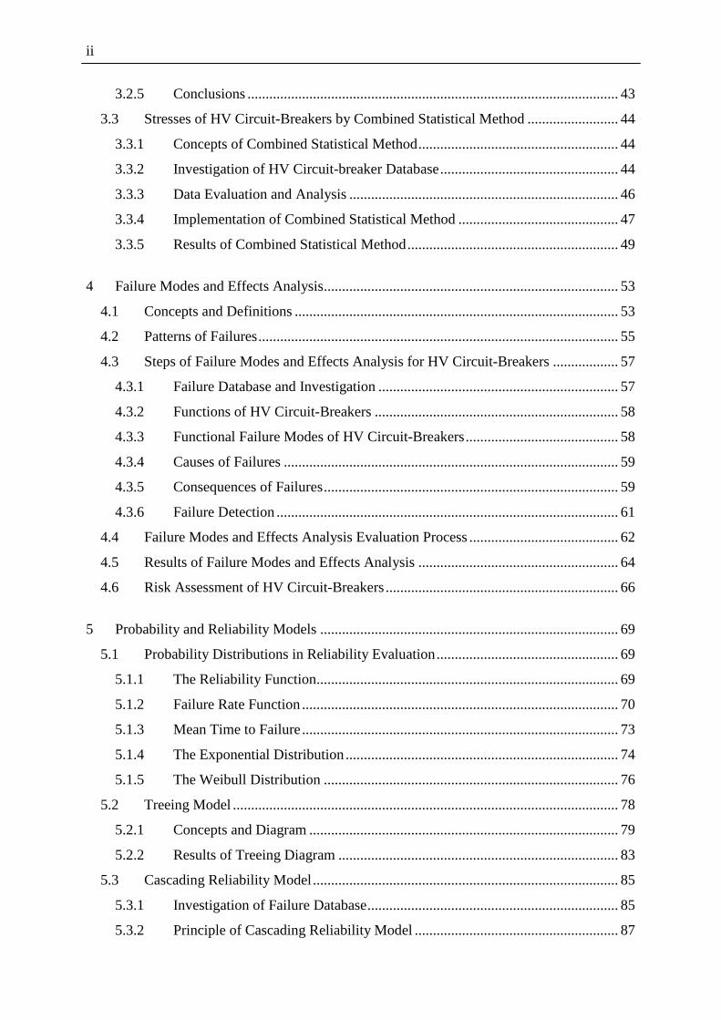
ii
3.2.5 Conclusions ...................................................................................................... 43
3.3 Stresses of HV Circuit-Breakers by Combined Statistical Method ......................... 44
3.3.1 Concepts of Combined Statistical Method....................................................... 44
3.3.2 Investigation of HV Circuit-breaker Database................................................. 44
3.3.3 Data Evaluation and Analysis .......................................................................... 46
3.3.4 Implementation of Combined Statistical Method ............................................ 47
3.3.5 Results of Combined Statistical Method.......................................................... 49
4 Failure Modes and Effects Analysis................................................................................. 53
4.1 Concepts and Definitions ......................................................................................... 53
4.2 Patterns of Failures................................................................................................... 55
4.3 Steps of Failure Modes and Effects Analysis for HV Circuit-Breakers ..................57
4.3.1 Failure Database and Investigation .................................................................. 57
4.3.2 Functions of HV Circuit-Breakers ................................................................... 58
4.3.3 Functional Failure Modes of HV Circuit-Breakers.......................................... 58
4.3.4 Causes of Failures ............................................................................................ 59
4.3.5 Consequences of Failures................................................................................. 59
4.3.6 Failure Detection .............................................................................................. 61
4.4 Failure Modes and Effects Analysis Evaluation Process ......................................... 62
4.5 Results of Failure Modes and Effects Analysis ....................................................... 64
4.6 Risk Assessment of HV Circuit-Breakers................................................................ 66
5 Probability and Reliability Models .................................................................................. 69
5.1 Probability Distributions in Reliability Evaluation.................................................. 69
5.1.1 The Reliability Function................................................................................... 69
5.1.2 Failure Rate Function ....................................................................................... 70
5.1.3 Mean Time to Failure....................................................................................... 73
5.1.4 The Exponential Distribution........................................................................... 74
5.1.5 The Weibull Distribution ................................................................................. 76
5.2 Treeing Model .......................................................................................................... 78
5.2.1 Concepts and Diagram ..................................................................................... 79
5.2.2 Results of Treeing Diagram ............................................................................. 83
5.3 Cascading Reliability Model.................................................................................... 85
5.3.1 Investigation of Failure Database..................................................................... 85
5.3.2 Principle of Cascading Reliability Model ........................................................ 87
iii
5.3.3 Results of Investigation.................................................................................... 88
5.3.4 Conclusions ...................................................................................................... 94
6 The Application of Markov Model .................................................................................. 95
6.1 Principles of Markov Model .................................................................................... 95
6.2 Reliability Parameters .............................................................................................. 98
6.3 Parallel Markov Model for HV Circuit-Breakers .................................................... 99
6.4 Matrix Approach .................................................................................................... 100
6.5 Results of Markov Model....................................................................................... 101
6.6 Conclusions ............................................................................................................ 106
7 Cost Structure and Maintenance Optimization .............................................................. 109
7.1 Cost Structure Determination................................................................................. 109
7.2 Maintenance Optimization ..................................................................................... 115
7.2.1 Optimal Maintenance Frequency ................................................................... 116
7.3 Reliability under Preventive Maintenance ............................................................. 122
7.3.1 Concepts of Preventive Maintenance............................................................. 122
7.3.2 Application of Preventive Maintenance to HV Circuit-Breakers .................. 124
7.3.3 Preventive Maintenance during Wear-out Period .......................................... 127
7.3.4 Consideration of Optimal Preventive Maintenance during Wear-out Period 129
8 Conclusions .................................................................................................................... 135
Bibliography........................................................................................................................... 139
List of Symbols and Abbreviations........................................................................................ 145
Appendix A The Transformation Method Used for Decision Matrix Approach................ 147
Appendix B The FMEA Evaluation of SF6 Circuit-Breakers ............................................ 149
B1: The FMEA evaluation based on the functional failures: SF6 circuit-breakers....... 149
B2: The FMEA evaluation based on component failures: SF6 circuit-breakers ........... 153
Appendix C Two-dimensional Diagrams of Treeing Model .............................................. 155
Appendix D The Decision Matrix of HV Circuit-Breaker’s Main Components................ 157
Appendix E Zusammenfassung in Deutsch........................................................................ 161

iv
1. Introduction 1
1 Introduction
1.1 Motivation
Due to the deregulation of electricity markets, reliability, stability and availability of power
systems must be improved in order to increase the competitiveness of electricity markets. In
order to improve such aspects, power systems should be operated with minimal abnormal
conditions and those conditions must be cleared as soon as possible. Therefore, HV circuit-
breakers, designed to interrupt faulted conditions, have played an important role in power
systems over 100 years since the first introduction of oil circuit-breakers.
Although the technology of an interrupting medium used in HV circuit-breakers has not been
considerably changed since the introduction of SF6 circuit-breakers in 1960s, the development
and studies in other areas, such as, materials, structures, arc models, monitoring, maintenance
techniques and asset management are still continued. At present, HV circuit-breakers are
basically designed to fit in the networks for any applications; for instance, capacitance
switching, line closing, shunt reactor switching, transformer switching and generator
protection. It is believed that designing general HV circuit-breakers to fit all purposes is cost
effective and easy to maintain. However, it is found that there are many over-designed HV
circuit-breakers installed in the networks during the past 30 years.
It is believed that the most practical and realistic method to study HV circuit-breaker
reliability is a statistical method. Worldwide surveys of HV circuit-breakers, 63 kV and above
had been carried out by CIGRE 13.06 in 1974-1977 for the first phase [1] and 1988-1991 for
the second phase [2]. The first survey focused on all types of HV circuit-breakers, whereas
the second survey focused only on single-pressure SF6 HV circuit-breakers. The comparison
represented that single-pressure SF6 circuit breakers have less major failure rate than older-
technology circuit breakers. Nevertheless, the minor failure rate of single-pressure SF6 circuit
breakers is higher than older-technology circuit breakers [3]. It is concluded from the second
survey that the minor failures result from operating mechanism, SF6 tightness, electrical
auxiliary and control circuits. Stresses of HV circuit-breakers in terms of loading current and

1. Introduction 2
short-circuit current (123 kV, 245 kV and 420 kV) during operation in the networks of
German utilities are also investigated and studied [4].
As the number of minor failures increase, the issues of how to conduct better maintenance are
becoming interesting. It cannot be avoided that better maintenance comes with the higher
maintenance costs which are not desirable for utilities. Hence, it is very challenging for
engineers to improve the maintenance programs while keeping the maintenance costs at an
acceptable level. This is among the most discussed issues in the asset management area, since
maintenance costs are considered as the large part of the operation costs.
There is some literature proposing the HV circuit-breaker optimal maintenance models but
most of them present only the strategies without the references from the failure databases. It is
still a challenge to design and investigate the reliability and maintenance models with
reference to the failure database collected from utilities. In addition, with the combination of
risk assessment, it is possible to design the reasonable optimal maintenance programs.
Influences of HV circuit-breaker specifications to the main components are of interest, since
they are the keys to investigate cost structure. As a result, it can lead to the optimal design of
HV circuit-breakers.
1.2 Research Objectives
The maintenance programs of HV circuit-breakers have been long performed by using the
manufacture guidelines and experiences of operators. They have hardly been proved that they
are really effective in terms of performance and costs. With emerge of deregulation electricity
markets, maintenance costs considered as the large part of operation costs of utilities should
be reduced in order to keep competitiveness of utilities.
To design new and optimal maintenance programs, it requires the knowledge of failure
database analysis, failure modes and effects analysis, reliability investigation and risk
assessment. The objectives of this work are mainly comprised of those mentioned aspects.
The failure database collected from utilities is deeply investigated to establish the
probabilistic models. These models can represent the probability of failures and how the

1. Introduction 3
failures are developed during the lifetime of HV circuit-breakers. For instance, the treeing
model of failures shows the distribution of failures from the first to the following failures in
any subsequent years. The cascading reliability model is an extension of treeing model to
investigate the reliability of HV circuit-breakers after consecutive failures. In addition, the
application of the Markov model can represent how the components of HV circuit-breakers
fail.
One of the main objectives of this work is failure modes and effects analysis of HV circuit-
breakers. This is the technique used to investigate failures and consequences of HV circuit-
breakers with reference to their functions and their components. The result of the
investigation represents the severity ranking of failures, which is important for the asset
managers to make decisions as to which failures must be intensively taken into account. The
consequence of this analysis results in risk assessment of HV circuit-breakers which can be
used to design the asset management.
Other objectives of this work dealing with asset management are cost structure analysis and
maintenance optimization. Cost structure analysis is able to breakdown the costs of HV
circuit-breakers with regard to the specifications and the components. Consequently, it
enables manufacturers to design the optimal HV circuit-breakers based on this cost analysis.
The “when and how” to perform maintenance tasks of HV circuit-breakers to increase the
reliability are of interest and are included in maintenance optimization.
1.3 Thesis Organization
The thesis contributions can be mainly divided into three phases: failure modes and effects
analysis, probabilistic models and maintenance optimization. The extra phase is the
investigation of stresses of HV circuit-breakers from the simulation and the statistical method.
The organization of this thesis can be described as followed:
• Fundamentals of HV circuit-breakers composed of functions and components of HV
circuit-breakers, types of HV circuit-breakers and switching transients are represented in
Chapter 2.

1. Introduction 4
• Chapter 3 represents the switching stresses of HV circuit-breakers. In this chapter, the
stresses of HV circuit-breakers regarding different types of applications are investigated
by simulation method. The other stresses regarding the number of faults and their
severity are investigated by using statistical method.
• Based on the failure database developed by the Institute of Power Systems, Darmstadt
University of Technology, it is possible to investigate failures of HV circuit-breakers by
using a failure modes and effects analysis method. The chapter 4 describes how to
conduct this process and presents the result of investigation. The risk assessment is also
considered in this chapter.
• The fundamentals of probability and reliability are first introduced in chapter 5. Then
developed models, a treeing model and a cascading reliability model are introduced.
With these models, the reliability and probability of HV circuit-breakers subject to
failures can be determined.
• The application of Markov process used to investigate steady-state probabilities is
introduced in chapter 6. The parallel Markov model for HV circuit-breakers is developed
to examine the state probabilities. Different types of HV circuit-breakers with different
driving mechanisms are taken into consideration.
• Chapter 7 is the last part of this thesis representing cost structure analysis and
maintenance optimization. A decision matrix approach is implemented in order to figure
out the importance of parameters relating to costs of HV circuit-breakers. Apart from
cost structure analysis method, maintenance optimization by using different methods is
introduced in this chapter.
• Finally, the conclusion is made in chapter 8 to summarize the results of this thesis and to
propose the direction of the future development.
2. Fundamentals of HV Circuit-Breakers
5
2 Fundamentals of HV Circuit-Breakers
2.1 Functions and Components of HV Circuit-Breakers
HV circuit-breakers are among the most important equipment in power systems. They are
designed to use as interrupting devices both in normal operation and during faults. It is
expected that HV circuit-breakers must be operated in any applications without problems.
Moreover, it is expected that they must be ready to be operated at anytime, even after a long
period of non-operating time. The main functions of HV circuit-breakers can be categorized
into four functions:
• Switching-off operating currents
• Switching-on operating currents
• Short-circuit current interruption
• Secure open and closed position
Apart from the main functions, they are required to fulfil the physical requirements as
follows:
• Behave as a good conductor during a closed position and as a good isolator during an
open position.
• Change from the closed to open position in a short period of time.
• Do not generate overvoltages during switching.
• Keep high reliability during operation.
More details of HV circuit-breaker functions and requirements under special conditions can
be reviewed in [5], [6] and [7]. Components of HV circuit-breakers regarding basic functions
can be divided into five groups [8]:
1. Insulation:
The electric insulation of HV circuit-breakers is provided by a combination of gaseous, liquid
and solid dielectric materials. The failure of insulation can lead to severe damage such as

2. Fundamentals of HV Circuit-Breakers 6
flashover between phases, to ground or across the opening poles resulting in major repair or
replacement. In order to prevent such failures, the insulation must be maintained and
monitored. For example, the quantity of insulating medium must be continuously monitored;
the quality of insulation has to be checked by diagnostic techniques periodically and the
insulation distance should be monitored by using position transducers and visual inspection.
2. Current carrying:
The current carrying parts are significant components that assure the flowing of current in the
closed position. The failure of these parts can lead to catastrophic events such as contact
welding and severe deterioration of the insulation system. It is however found that it takes
several years until the contact degradation process reaches the final states. Practically, the
most contact problems can be prevented by using periodic diagnostic testing. The techniques
of current carrying testing can be accomplished by monitoring or diagnostic testing of contact
resistance, temperature of contacts, load current and content of gas decomposition.
3. Switching:
During operation of HV circuit-breakers, they are subject to electrical, thermal and
mechanical stresses. It is required that they should be able to make and break large amount of
power without causing failures. The parameters used to monitor and diagnose switching are
composed of position of primary contacts, contact travel characteristics, operating time, pole
discrepancy in operating times, arcing time and arcing contact wear. Contact travel
characteristics are the most widely used parameters in periodic testing in order to investigate
the contact movement.
4. Operating mechanism:
The operating mechanism is a part used to move contacts from open to closed position or
inversely. The operating mechanism failures account for a large proportion of total failures of
HV circuit-breakers. For example, leakage of oil and gas in the hydraulic and pneumatic
systems is very common but it can be handled without system interruption. On the other hand,
breakdown of shafts, rods and springs could lead to serious failures resulting in the
interruption of systems.
2. Fundamentals of HV Circuit-Breakers
7
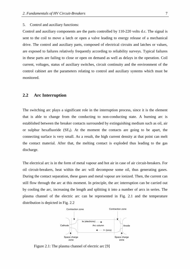
5. Control and auxiliary functions:
Control and auxiliary components are the parts controlled by 110-220 volts d.c. The signal is
sent to the coil to move a latch or open a valve leading to energy release of a mechanical
drive. The control and auxiliary parts, composed of electrical circuits and latches or values,
are exposed to failures relatively frequently according to reliability surveys. Typical failures
in these parts are failing to close or open on demand as well as delays in the operation. Coil
current, voltages, status of auxiliary switches, circuit continuity and the environment of the
control cabinet are the parameters relating to control and auxiliary systems which must be
monitored.
2.2 Arc Interruption
The switching arc plays a significant role in the interruption process, since it is the element
that is able to change from the conducting to non-conducting state. A burning arc is
established between the breaker contacts surrounded by extinguishing medium such as oil, air
or sulphur hexafluoride (SF6). At the moment the contacts are going to be apart, the
connecting surface is very small. As a result, the high current density at that point can melt
the contact material. After that, the melting contact is exploded thus leading to the gas
discharge.
The electrical arc is in the form of metal vapour and hot air in case of air circuit-breakers. For
oil circuit-breakers, heat within the arc will decompose some oil, thus generating gases.
During the contact separation, these gases and metal vapour are ionized. Then, the current can
still flow through the arc at this moment. In principle, the arc interruption can be carried out
by cooling the arc, increasing the length and splitting it into a number of arcs in series. The
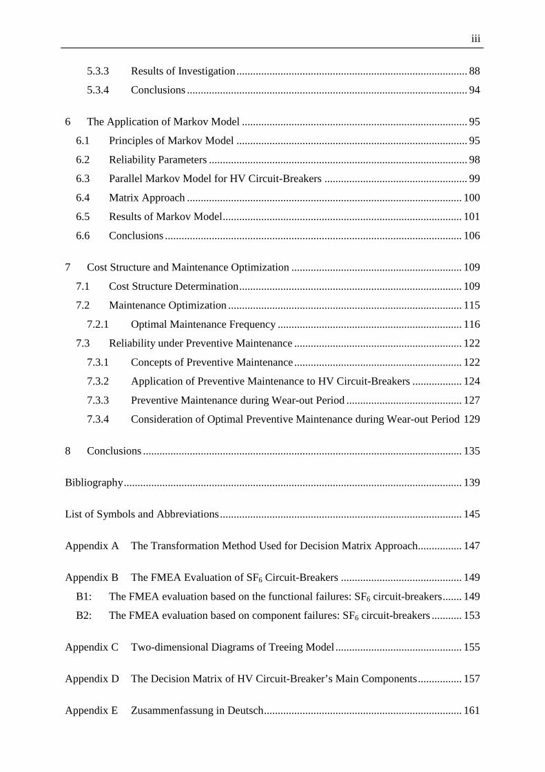
plasma channel of the electric arc can be represented in Fig. 2.1 and the temperature
distribution is depicted in Fig. 2.2
AnodeCathode Arc column
Contraction zone Contraction zone
Space charge
zone
Space charge
zone
Ie (electrons)
I+ (ions)
Figure 2.1: The plasma channel of electric arc [9]

2. Fundamentals of HV Circuit-Breakers 8
Voltage
Gap length
Uarc
Uanode
Ucolumn
Ucathode
Figure 2.2: The potential distribution along an arc channel [9]
The voltage drop near the cathode region is normally around 10-25 volts, while the voltage
drop near anode is around 5-10 volts. The voltage drop in the arc column depends on the
types of gases, gas pressure, the magnitude of arc current and the length of column [10].
2.3 Circuit-Breaker Classification
According to many criteria, circuit-breakers can be classified into many groups as follows:
• Circuit-breaker types by voltage class:
The classification of circuit-breakers regarding voltage class can be divided into two groups:
low voltage circuit-breakers with rated voltages up to 1000 volts and high voltage circuit-
breakers with rated voltages of 1000 volts and above. The second group, high voltage circuit-
breakers, can be further subdivided into two groups: circuit-breakers with rated 50 kV and
below and those with rated 123 kV and above.
• Circuit-breaker types by installation:
Circuit-breakers can be classified in terms of installation into two types: indoor and outdoor
installations. Practically, the only differences between those two types are the packaging and
the enclosures.
• Circuit-breaker types by external design:
Outdoor circuit-breakers can be classified with respect to structure design into two types:

2. Fundamentals of HV Circuit-Breakers
9
dead and live tank types. Dead tank circuit-breakers are the circuit-breakers of which the
enclosures and interrupters are grounded and located at ground level, as shown in Fig. 2.3.
This type of circuit-breaker is widely used in the United States. Live tank circuit-breakers are
circuit-breakers equipped with the interrupters above the ground level, as shown in Fig. 2.4.
Their interrupters have the potential.
Figure 2.3: Dead tank circuit-breaker (Source: Manitoba, Canada)
Figure 2.4: Live tank circuit-breaker (Source: ABB AG, Switzerland)
• Circuit-breaker types by interrupting medium:
The interrupting mediums are the main factors in designing circuit-breakers. The technology
of air and oil interrupting mediums for circuit-breakers was first developed 100 years ago.

2. Fundamentals of HV Circuit-Breakers 10
These types of circuit-breakers are still in operation but there is no further development, since
they cannot fulfil the higher ratings of power systems nowadays. In addition, there are issues
as environmental problems and as to relatively low reliability. The new generation of
interrupting mediums is focused on vacuum and sulfurhexafluoride (SF6). Vacuum circuit-
breakers are predominant in medium voltage levels, whereas SF6 circuit-breakers are widely
used in high voltage levels.
• Circuit-breaker types by operation:
The main purpose of HV circuit-breakers is interrupting abnormal conditions. Nevertheless,
different applications of HV circuit-breakers must be taken into account. The applications of
HV circuit-breakers can be classified as follows:
- Capacitance switching: capacitor banks and unloaded cable switching
- Line closing: overhead transmission line switching
- Shunt reactor switching
- Transformer switching
- Generator switching
2.4 Types of Circuit-Breakers
Circuit-breakers can be classified according to interrupting mediums into four categories:
2.4.1 Oil Circuit-Breakers
Oil circuit-breakers are the most fundamental circuit-breakers which were first developed in
1900s. The first oil circuit-breaker was developed and patented by J. N. Kelman in the United
States. Oil has an excellent dielectric strength which enables itself not only to be used as an
interrupting medium but also as insulation within the live parts. The interrupting technique of
oil circuit-breakers is called “self-extinguishing”, since the oil can produce a high pressure
gas when it is exposed to heat resulting from arc. In other words, arc can be cooled down by
the gas produced proportional to arc energy. During the arc interruption, the oil forms a
bubble comprising mainly hydrogen. It is found that arc burning in hydrogen gas can be

2. Fundamentals of HV Circuit-Breakers
11
extinguished faster than other types of gases. However, hydrogen cannot be used as
interrupting medium, as it is not practical to handle. Oil circuit-breakers can be divided
according to methods of arc interruption into two types: bulk oil and minimum oil types.
2.4.1.1 Bulk oil type
The main contacts and live parts are immersed in oil which serves as an interrupting medium
and insulates the live parts. Plain-break circuit-breakers are considered as bulk oil type, since
the arc is freely interrupted in oil. This type of circuit-breaker contains a large amount of oil
and requires a large space. It could cause environmental problems after an explosion. It is
therefore limited to the low voltage level. An example of a bulk oil circuit-breaker and its
components is represented in Fig. 2.5.
Figure 2.5: Bulk oil circuit-breaker (Source: Allis Chalmers Ltd.)
1. bushing 6. plunger guide
2. oil level indicator 7. arc control device
3. vent 8. resistor
4. current transformer 9. plunger bar
5. dashpot

2. Fundamentals of HV Circuit-Breakers 12
2.4.1.2 Minimum oil type
This type of oil circuit-breaker was developed in Europe, due to requirement to reduce
utilized space and cost of oil. In comparison to the bulk oil type, for the minimum oil type the
volume of oil is reduced and used only in an explosion chamber. The other difference from
the bulk oil type is the insulation, which is made of porcelain or solid insulating material.
Single-break minimum oil circuit-breakers are used in the voltage levels of 33-132 kV. When
higher ratings are required, the multi-break type is then applied with a combination of
resistors and capacitors. These resistors and capacitors are applied in order to provide
uniformity to the voltage distribution.
2.4.2 Air-Blast Circuit-Breakers
The arc interruption of air-blast circuit-breakers is carried out by introducing the high-
pressure air flow in axial or cross directions as shown in Fig. 2.6. In axial type, the arc is
cooled down in an axial direction until the ionisation is brought down to zero level. The
current is then interrupted at this point. In contrast to the axial type, the cross type will
compress the air and blow into an arc-chute compartment.
(a) (b)
Con
tact
Contact Contact
Co
ntac
t
Gas flow direction
Gas
flo
w d
irect
ion
Gas
flo
w d
irect
ion
Figure 2.6: Air blast direction: (a) axial direction, (b) cross direction
The performance of air-blast circuit-breakers depends on many factors, for example, operating
pressure, the nozzle diameter and the interrupting current. The advantages of air-blast circuit-
breakers can be listed as follows [11]:
2. Fundamentals of HV Circuit-Breakers
13
• Cheap interrupting medium
• Chemical stability of air
• Reduction of erosion of contacts from frequent switching operations
• Operation at high speed
• Short arcing time
• Being able to be operated in fire hazard locations
• Reduction of maintenance frequency
• Consistent breaking time
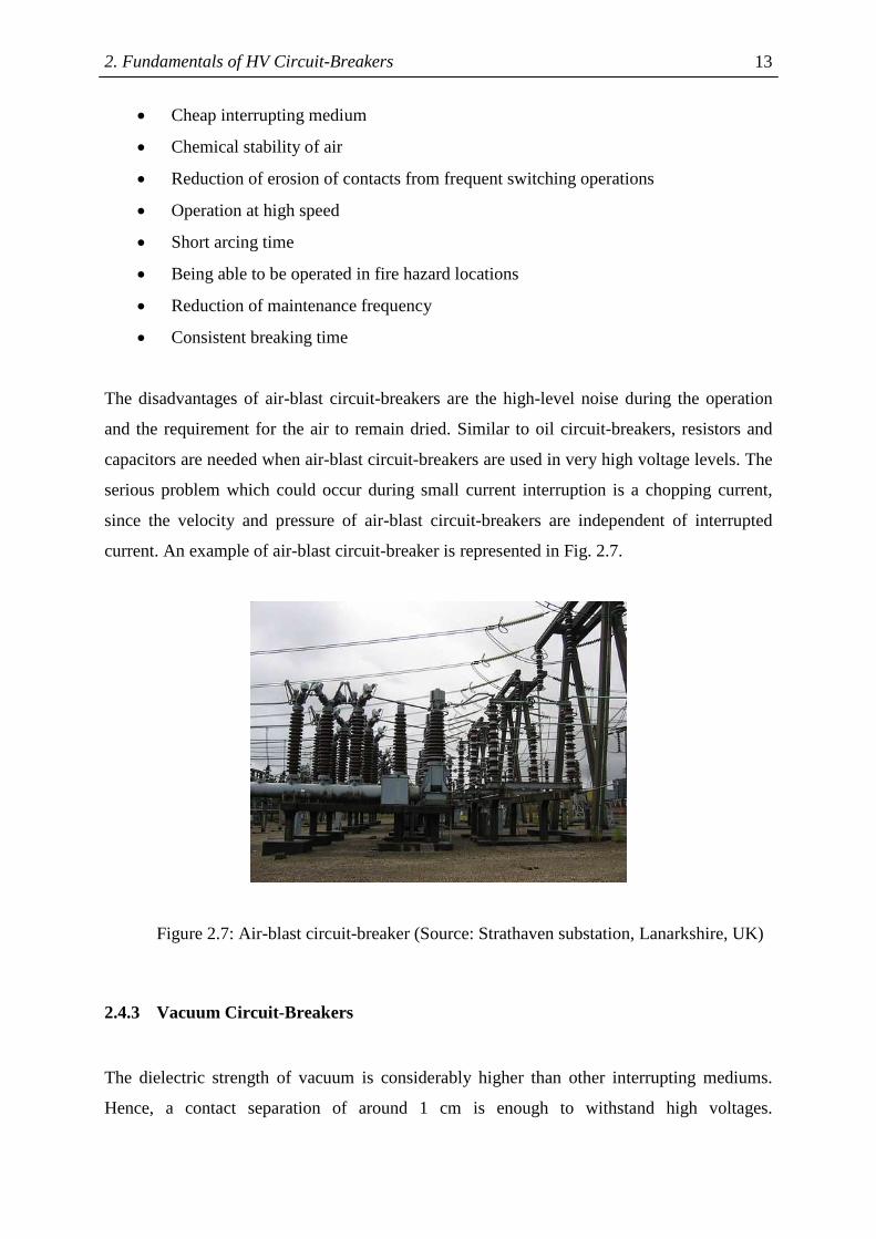
The disadvantages of air-blast circuit-breakers are the high-level noise during the operation
and the requirement for the air to remain dried. Similar to oil circuit-breakers, resistors and
capacitors are needed when air-blast circuit-breakers are used in very high voltage levels. The
serious problem which could occur during small current interruption is a chopping current,
since the velocity and pressure of air-blast circuit-breakers are independent of interrupted
current. An example of air-blast circuit-breaker is represented in Fig. 2.7.
Figure 2.7: Air-blast circuit-breaker (Source: Strathaven substation, Lanarkshire, UK)
2.4.3 Vacuum Circuit-Breakers
The dielectric strength of vacuum is considerably higher than other interrupting mediums.
Hence, a contact separation of around 1 cm is enough to withstand high voltages.
2. Fundamentals of HV Circuit-Breakers 14
Consequently, the power to open and close contacts can be significantly reduced compared
with other types of circuit-breakers. In addition, the rate of dielectric recovery of vacuum is
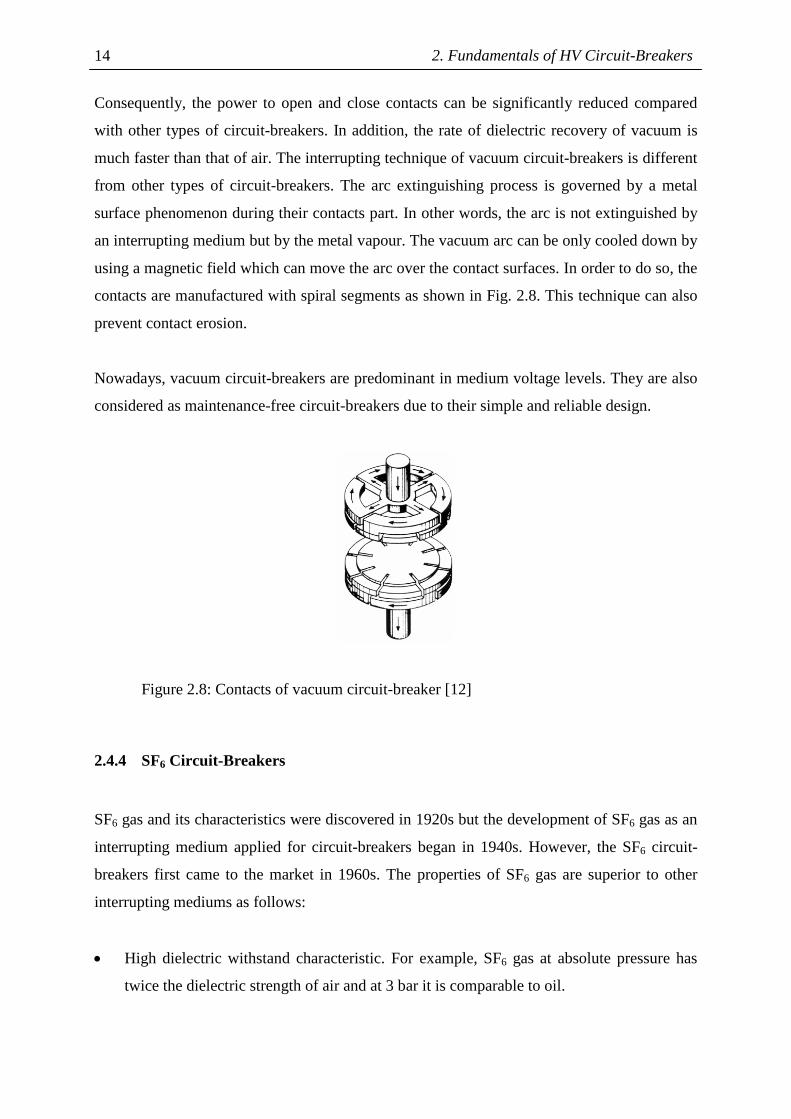
much faster than that of air. The interrupting technique of vacuum circuit-breakers is different
from other types of circuit-breakers. The arc extinguishing process is governed by a metal
surface phenomenon during their contacts part. In other words, the arc is not extinguished by
an interrupting medium but by the metal vapour. The vacuum arc can be only cooled down by
using a magnetic field which can move the arc over the contact surfaces. In order to do so, the
contacts are manufactured with spiral segments as shown in Fig. 2.8. This technique can also
prevent contact erosion.
Nowadays, vacuum circuit-breakers are predominant in medium voltage levels. They are also
considered as maintenance-free circuit-breakers due to their simple and reliable design.
Figure 2.8: Contacts of vacuum circuit-breaker [12]
2.4.4 SF6 Circuit-Breakers
SF6 gas and its characteristics were discovered in 1920s but the development of SF6 gas as an
interrupting medium applied for circuit-breakers began in 1940s. However, the SF6 circuit-
breakers first came to the market in 1960s. The properties of SF6 gas are superior to other
interrupting mediums as follows:
• High dielectric withstand characteristic. For example, SF6 gas at absolute pressure has
twice the dielectric strength of air and at 3 bar it is comparable to oil.
2. Fundamentals of HV Circuit-Breakers
15
• High thermal conductivity and short thermal time constant (1000 times shorter than air)
resulting in better arc quenching.
• Arc voltage characteristic is low thus resulting in reduced arc-removal energy.
• At normal conditions, SF6 is inert, non-flammable, non-corrosive, odourless and non-
toxic. However, at the temperature over 1000°C, SF6 decomposes to gases including
S2F10 which is highly toxic. Fortunately, the decomposition products recombine abruptly
after arc extinction (when the temperature goes down).
The problem of moisture from the decomposition products must be considered. The moisture
can be absorbed by a mixture of soda lime (NaOH + CaO), activated alumina (dried Al2O3) or
molecular sieves. The other problem is the condensation of SF6 at high pressures and low
temperatures. For example, at a pressure of 14 bars, SF6 liquefies at 0°C. In the areas with low
ambient temperature such as Canada, Scandinavian countries and Russia, gas heaters must be
utilized. The other solution is the introduction of gas mixtures such as nitrogen (N2). Although
the gas mixture of SF6/N2 can be used in the low ambient temperature, the dielectric withstand
capability and arc interruption performance are reduced. For example, the short-circuit
capacity rating of 50kA is reduced to 40kA. The development and types of SF6 circuit-
breakers can be represented as follows:
2.4.4.1 Double-pressure SF6 circuit-breakers
This type is developed by using principles similar to air-blast circuit-breakers. The contacts
are located inside the compartment filled with SF6 gas. During the arc interruption, the arc is
cooled down by compressed SF6 from a separate reservoir. After the interruption, SF6 gas is
pumped back into the reservoir. This reservoir must be equipped with heating equipment to
ensure that the SF6 will not liquefy. However, failures of heating equipment can result in this
type being unable to operate as circuit-breakers. This type of SF6 circuit-breaker is rarely used
in the market nowadays because of its high failure probability.
2.4.4.2 Self-blast SF6 circuit-breakers
The interrupting chamber of this type of circuit-breaker is divided into two main
compartments with the same pressure (around 5 atm). During the arc interruption, the gas
pressure in the arcing zone is heated resulting in high pressure. This high pressure gas from
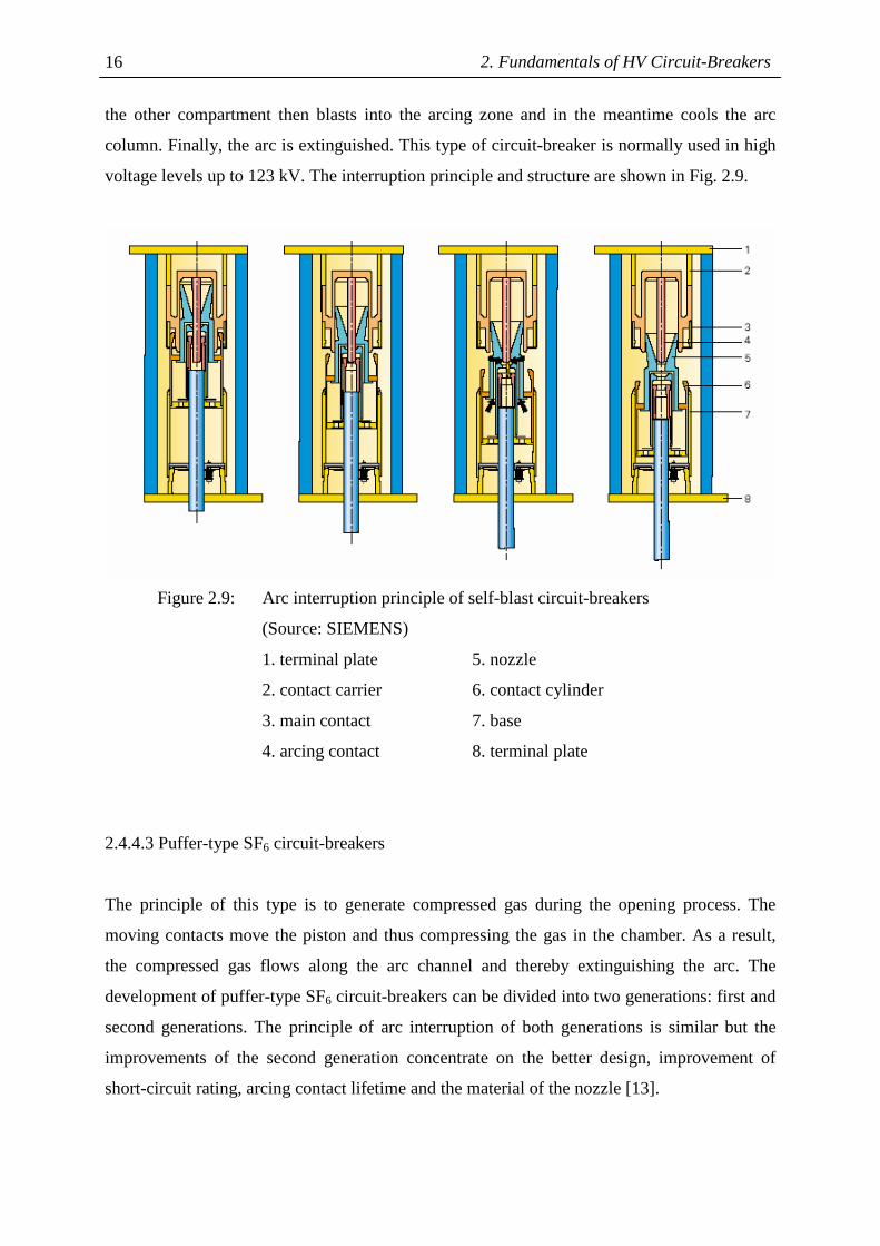
2. Fundamentals of HV Circuit-Breakers 16
the other compartment then blasts into the arcing zone and in the meantime cools the arc
column. Finally, the arc is extinguished. This type of circuit-breaker is normally used in high
voltage levels up to 123 kV. The interruption principle and structure are shown in Fig. 2.9.
Figure 2.9: Arc interruption principle of self-blast circuit-breakers
(Source: SIEMENS)
1. terminal plate 5. nozzle
2. contact carrier 6. contact cylinder
3. main contact 7. base
4. arcing contact 8. terminal plate
2.4.4.3 Puffer-type SF6 circuit-breakers
The principle of this type is to generate compressed gas during the opening process. The
moving contacts move the piston and thus compressing the gas in the chamber. As a result,
the compressed gas flows along the arc channel and thereby extinguishing the arc. The
development of puffer-type SF6 circuit-breakers can be divided into two generations: first and
second generations. The principle of arc interruption of both generations is similar but the
improvements of the second generation concentrate on the better design, improvement of
short-circuit rating, arcing contact lifetime and the material of the nozzle [13].
2. Fundamentals of HV Circuit-Breakers
17
Since the gas has to be compressed, the puffer-type SF6 circuit-breaker must have a strong
operating mechanism. For example, when large current such as three-phase fault is
interrupted, the opening speed of circuit-breakers is slowed down because of thermal
pressure. The operating mechanism should have adequate energy to move the contacts apart.
Consequently, the reliable operating mechanisms dominate the costs of circuit-breakers.
At present, SF6 circuit-breakers are predominant in high voltage levels with the high short-
circuit capability up to 63 kA. They can be used as dead tank circuit-breakers, live tank
circuit-breakers and in gas insulated substation (GIS).
2.5 Switching Transients and Applications of HV Circuit-Breakers
Apart from normal load current interruption, the other main purpose of HV circuit-breakers is
interrupting short-circuit currents. In addition, different applications of HV circuit-breakers
must be taken into account, such as small inductive current interruption, capacitive current
interruption, short-line fault interruption and generator protection. The applications of HV
circuit-breakers can be summarized as follows:
2.5.1 Three-Phase Short-Circuit Interruption at Terminal
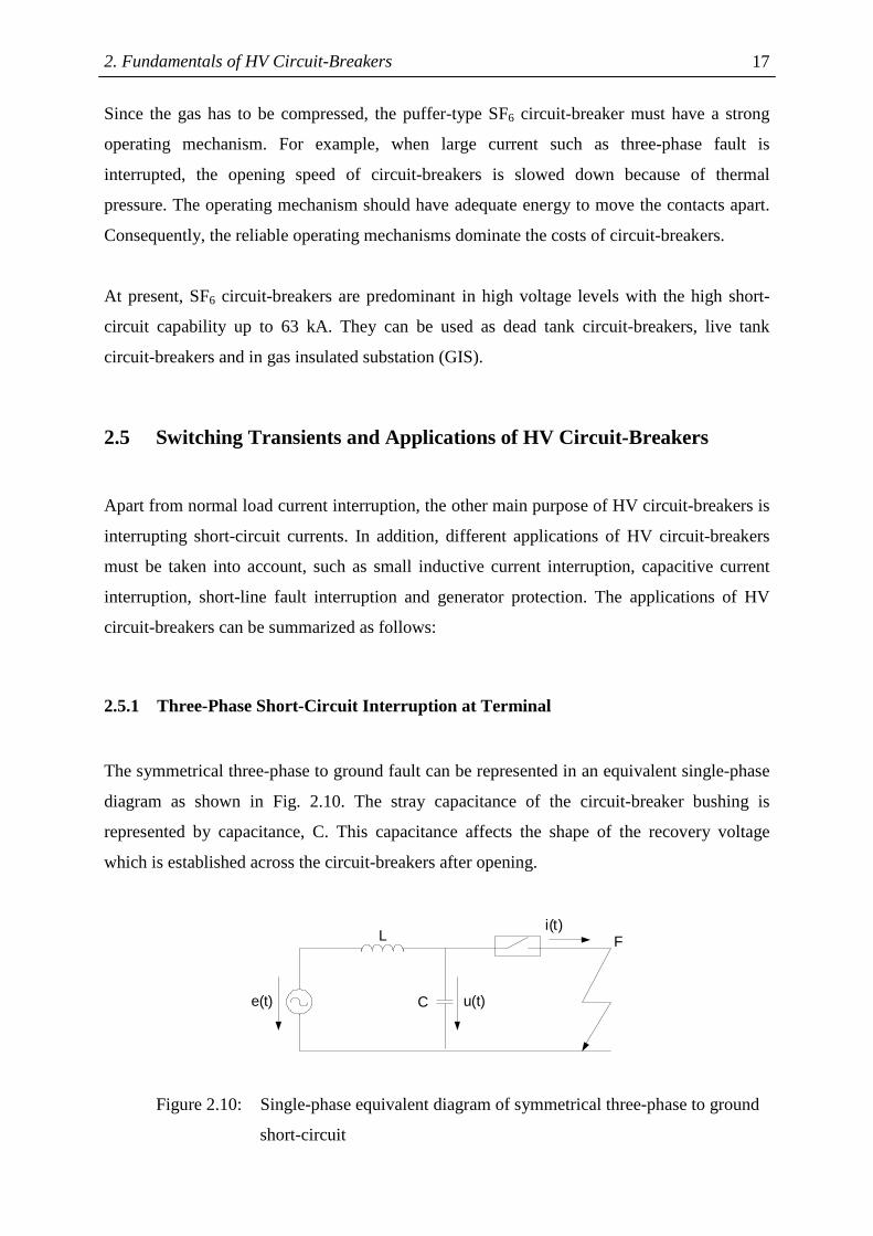
The symmetrical three-phase to ground fault can be represented in an equivalent single-phase
diagram as shown in Fig. 2.10. The stray capacitance of the circuit-breaker bushing is
represented by capacitance, C. This capacitance affects the shape of the recovery voltage
which is established across the circuit-breakers after opening.
L
e(t) C
i(t)
u(t)
F
Figure 2.10: Single-phase equivalent diagram of symmetrical three-phase to ground
short-circuit

2. Fundamentals of HV Circuit-Breakers 18
There is a short-circuit current at point F and the circuit-breaker has to interrupt at current
zero. Assume that the supply voltage is equal toe(t) = Ecosωt . The circuit voltage equation
when the circuit-breaker is opened can be represented in the form
di 1
L + idt = Ecosωtdt C∫ (2.1)
By using the Laplace transformation with the natural angular frequency 0ω = 1/ LC , the
recovery voltage can be represented as
0u(t) = E(-cosω t + cosωt) (2.2)
At the instant after short-circuit interruption, the time t is very short (t < 1 ms) and thus
resulting incosωt = 1. The recovery voltage can be approximated in the form
0u(t) = E(1 - cosω t) (2.3)
The possible maximum recovery voltage without damping is 2E after time π / LC .
Practically, the maximum recovery voltage is less than 2E because of resistance and system
losses.
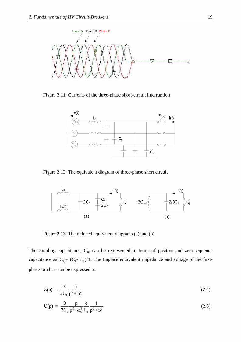
The switching sequence depends on the neutral grounding. The example of an isolated neutral
system with three-phase short-circuit interruption can be explained from Fig. 2.11. The arc
interruption is first taking place at current zero of phase A, while phase B and C are still
arcing. After 90o from the first phase to clear (phase A), the other phases (B and C) are then
simultaneously interrupted. The equivalent diagram of three-phase short circuit in an isolated
neutral system is represented in Fig. 2.12. The first phase is going to be interrupted, then the
reduced equivalent diagram can be expressed as in Fig. 2.13a and 2.13b.
2. Fundamentals of HV Circuit-Breakers
19
Phase A Phase B Phase C
Figure 2.11: Currents of the three-phase short-circuit interruption
L1
Cg
C0
i(t)e(t)
Figure 2.12: The equivalent diagram of three-phase short circuit
L1
L1/22Cg
2C0
C0
i(t)
3/2L1
i(t)
2/3C1
(a) (b)
Figure 2.13: The reduced equivalent diagrams (a) and (b)
The coupling capacitance, Cg, can be represented in terms of positive and zero-sequence
capacitance as g 1 0C = (C - C )/3. The Laplace equivalent impedance and voltage of the first-
phase-to-clear can be expressed as
2 21 0
3 pZ(p) =
2C p +ω (2.4)
2 2 2 21 10
ˆ3 p e 1U(p) =
2C Lp +ω p +ω (2.5)

2. Fundamentals of HV Circuit-Breakers 20
It is assumed that 2 20ω >> ω , then the voltage of the first-phase-to-clear after transformation is
[ ]03
ˆu(t) = e -cosω t + cosωt2
(2.6)
It can be seen from Eq. 2.6, that the first phase to clear factor, defined as the ratio between the
voltage across the first clearing phase and the uninterrupted phase voltage, is 1.5. The first
phase to clear factors in case of resonant earthed and solidly neutral are less than 1.5
depending on the ratio between positive and zero sequence impedances. When short-circuit
occurs far from the terminal, the transient recovery voltage will have more than one frequency
component. The frequency of source side and line side must be taken into account resulting in
double frequency transient recovery voltage. In addition to transient recovery voltage, the rate
of rise of recovery voltage (RRRV) must be considered. According to IEC standard 62271-
100, circuit-breakers must be able to withstand RRRV up to 2 kV/µs. In some cases, for
example, short-line faults (section 2.5.4) of which RRRVs are higher than 2 kV/µs, the
protective capacitance must be implemented to reduce the steepness of recovery voltage.
2.5.2 Capacitive Current Interruption
Capacitive current interruption can generate overvoltages across circuit-breakers leading to
dielectric breakdown of circuit-breakers. The reason for the overvoltages can be explained by
the electrical charge effect at the capacitive loads such as capacitor banks, cables and
unloaded transmission lines. The equivalent single-phase circuit diagram and waveforms of
capacitive current interruption are depicted in Fig. 2.14.
L
e(t) C
i(t)
u(t)
us(t)
et) u(t)
us(t)
i(t)
Figure 2.14: Equivalent circuit diagram of capacitive current interruption
2. Fundamentals of HV Circuit-Breakers
21
Before the capacitive load is switched off, the capacitive load is fully charged equal to the
peak supply voltage. After half a cycle, the supply voltage is reversed thus making the voltage
across the circuit-breaker twice the peak value of the supply voltage. If the circuit-breaker
cannot withstand this voltage, a restrike takes place across the circuit-breaker resulting in a
high frequency current. The circuit-breaker is able to interrupt such current in a half cycle
later. At this moment, the voltage at the capacitor reaches 3 times that of the supply voltage. If
the circuit-breaker cannot withstand the voltage across itself, the restrike can take place again
with the voltage at the capacitor 5 times that of the supply voltage. The details of capacitive
current switching can be reviewed in [14].
Many applications of circuit-breaker interruption are considered as capacitive current
interruption, for example, interruption of no-load transmission lines, interruption of no-load
cables and switching-off capacitor banks. When the circuit-breaker is called upon to interrupt
the capacitive current (for example, no-load transmission line interruption), the load voltage is
higher than the supply voltage. This phenomenon is called Ferranti effect, leading to a voltage
jump at the supply side of the circuit-breaker.
2.5.2.1 Interruption of no-load transmission lines
The transmission lines are first switched off at the line side resulting in no-load transmission
lines. At this moment, only a charging current flows in the transmission lines and it charges
the capacitance of the transmission lines. After that, the circuit-breaker at the sending end is
called upon to switch off. The circuit-breaker is then stressed by the voltage rise at the supply
side and the oscillation at the line side. The recovery voltage across the circuit-breaker varies
from 2.0 to 3.0 p.u. depending on the ratio of positive-sequence to zero-sequence capacitance
(C1/C0). The relation of C1/C0 and the recovery voltages are represented in [15]. The geometry
of transmission lines and tower configurations affect the coupling capacitance between lines
and earth, thus leading to different voltage stresses on circuit-breakers.
2.5.2.2 Interruption of no-load cables
Interruption of no-load cables is similar to interruption of no-load transmission lines which
belongs to the case of capacitive current interruption. The difference is the interrupting
current, which is larger than the interrupting current of no-load transmission lines but smaller
2. Fundamentals of HV Circuit-Breakers 22
than the interrupting current of capacitor banks. The configurations of cables must be taken
into account. For example, the separate conductor with its own earth screen can be treated
similar to capacitor banks with an earthed neutral in a grounded system, since there is only an
effect of capacitance to ground.
2.5.2.3 Switching capacitor banks
Capacitor banks are used in power systems to improve voltage regulation and reduce losses
through reduction in reactive current or filter higher harmonics. Energizing a single capacitor
bank could generate inrush current with a high frequency. It is noted that the magnitude and
frequency of inrush current in the case of switching back-to-back capacitor banks are higher
[16]. Furthermore, energizing capacitor banks could lead to a pre-strike of the circuit-breaker
when the supply voltage reaches its peak before the contacts touch. The switching off three-
phase grounded capacitor banks in solidly grounded system can be treated as single phase
circuit. The maximum voltage across the circuit-breakers is 2 p.u. In case of switching-off
three-phase ungrounded capacitor banks, the trapped charge of the first-phase-to-clear must
be taken into account. As a result, the maximum voltage across the circuit-breakers could
reach 3 p.u.
2.5.3 Small Inductive Current Interruption
In case of a large short-circuit current interruption, the arc energy is high enough to keep the
arc column ionized until the arc is interrupted at natural current zero. On the other hand,
interrupting small inductive currents, such as unloaded currents of transformers and currents
of shunt reactors, can produce overvoltages according to chopping current effects. It can be
explained that the small inductive current is interrupted just before natural current zero, thus
inducing the high transient voltages (L di/dt⋅ ). Consequently, these transient voltages can
cause flashover on the insulation, such as bushings. The equivalent single-phase circuit
diagram and waveforms of small inductive current interruption are illustrated in Fig. 2.15.

2. Fundamentals of HV Circuit-Breakers
23
Le(t) C
i(t)
us(t)u(t)
et)
u(t)us(t)
i(t)
Figure 2.15: Equivalent circuit diagram of small inductive current interruption
The principle to calculate the voltages across circuit-breakers during current chopping is the
energy conversion before and after arc interruption. When the circuit-breaker interrupts an arc
current, the electromagnetic energy stored in the inductance L is transferred to electrical
energy in the capacitance C. The balance energy equation is as follows [17]:
2 20 0 0
1 1Li + Cu = E
2 2 (2.7)
where L, C Inductance, Capacitance
0i Current at the time of interruption
0u Voltage at the time of interruption
0E Total energy
After the interruption, the total energy and maximum voltage can be represented as:
2max 0
1Cu = E
2 (2.8)
2 2max 0 0
Lu = i + u
C (2.9)
It can be seen from equation 1.6 that the maximum voltage depends on the characteristic
impedance WZ = L/C of equipment. The examples of transient overvoltages regarding
switching shunt reactors and unloaded transformers can be reviewed in [18] and [19].

2. Fundamentals of HV Circuit-Breakers 24
2.5.4 Short-Line Fault Interruption
It is found that short-circuit current interruption far from the circuit-breakers from hundreds
of metres to a few kilometres could result in circuit-breaker breakdown. The very high
steepness (3 to 10 kV/µs) of recovery voltages after circuit-breaker interruption could result in
very high stress thus leading to thermal breakdown of the arc channel. The explanation of
short-line fault is illustrated in Fig. 2.16.
L
e(t) C uL
F
l
Line-side voltage
Source-side voltagee(t)
t
Figure 2.16: Equivalent circuit diagram of short line fault interruption
The transient recovery voltage after short-line fault interruption is composed of voltage
generated by the source-side voltage and the line-side voltage. The source-side voltage is the
gradually rising voltage with the (1-cosine) shape, whereas the line-side voltage has the saw-
toothed voltage shape with very high frequency. The starting voltage of the recovery voltage
and the line-side frequency can be represented as follows:
"L W W k
diu = Z = Z ω 2I
dt (2.10)
with "kI Short-circuit current
WZ Characteristic impedance of the line
ω Operating frequency
L
2 2
1f =
2π L C (2.11)
2. Fundamentals of HV Circuit-Breakers
25
where L2 and C2 are the equivalent series impedance and shunt capacitance of the line from
the circuit-breaker to the fault respectively. The saw-toothed voltage shape of the line-side is
originated by the reflection of travelling wave at the short-circuit point.
The short-line fault test is considered as the most severe short-circuit test and has been
included in the standard. The short-line fault tests are considered with respect to the short-
circuit rating of circuit-breakers. 75% and 90% short-line faults have been applied by IEC
standard.
2.5.5 Circuit-Breakers Installed for Generator Protection
Circuit-breakers for generator protection are installed between generators and step-up
transformers. The characteristics of faults near generators can be as described below:
• The recovery voltage has a very high rate of rise due to the small capacitance, C.
• The effect of the d.c. component of short-circuit current must be taken into account.
• The decay of the a.c. component depends on subtransient and transient time constants of
the generator.
• The d.c. component at the interrupting time could be higher than the peak value of the
a.c. component depending on the generator rating.
• The short-circuit current might not cross the zero for a period of time depending on the
load condition before interruption.
The generator circuit-breakers are designed to handle these conditions by introducing a high
arc voltage. The high arc voltage generates an additional resistance resulting in reduction of
the time constant of the fault. As a result, the fault can be interrupted with a reduced time
delay.
At present, this type of circuit-breaker is widely used to protect generators having ratings
from 100-1300 MVA. The interrupting capacities of SF6 generator circuit-breakers are around
63 kA to more than 200 kA, while air-blast circuit-breakers are applied for higher interrupting
capacities. The standard of the generator circuit-breakers can be found in [20]. The results of
testing and influence of cable connection was studied in [21].

2. Fundamentals of HV Circuit-Breakers 26
2.6 Summary of Reliability Surveys of HV Circuit-Breakers by CIGRE
The most important and internationally reliability surveys of HV circuit-breakers had been
carried out by CIGRE. The first enquiry had been performed during 1974-1977 from 102
companies in 22 countries. This enquiry focused on all types of HV circuit-breakers with
ratings of 63 kV and above. The total information of 77,892 breaker-years had been collected.
The second enquiry, focused only on single-pressure SF6 circuit-breakers, had been done
during 1988-1991 from 132 companies in 22 countries. The second enquiry contains 70,708
breaker-years and also focused on circuit-breakers with ratings of 63 kV and above. The
major and minor failures can be defined as follows:
• Major failure (MF): Complete failure of a circuit-breaker which causes the lack of one or
more of its fundamental functions. A major failure will result in immediate change in the
system operation conditions leading to removal from service for non-scheduled
maintenance (intervention required within 30 minutes).
• Minor failure (mF): Failure of a circuit-breaker other than a major failure or any failure,
even complete, of a constructional element or a subassembly which does not cause a
major failure of the circuit-breaker.
The major and minor failures at different voltage levels from both enquiries can be
summarized in Table 2.1 [22]. The short summary of the 2nd survey can be found in [23].
According to Table 2.1, the ratio between minor and major failures can be calculated and
represented in Table 2.2.
It can be concluded from the 2nd enquiry compared with the 1st enquiry that:
• The major failure rate of the single-pressure SF6 circuit-breakers is 60% lower than all
types of circuit-breakers from the 1st survey.
• The minor failure rate of the SF6 circuit-breakers is 30% higher than that of the first
survey. It is because of more signals of the monitoring systems and because of SF6
leakage problems
• The operating mechanism is subject to the most failures in the failure modes of “Does
not open or close on command” and “Locked in open or closed position”.

2. Fundamentals of HV Circuit-Breakers
27
Major failure rate (Failures per year)
Minor failure rate (Failures per year)
Voltage (kV)
1st Enquiry 1974-1977
2nd Enquiry 1988-1991
1st Enquiry 1974-1977
2nd Enquiry 1988-1991
All voltages 0.0158 0.0067 0.0355 0.0475
63-99 0.0041 0.0028 0.0165 0.0223
100-199 0.0163 0.0068 0.0417 0.0475
200-299 0.0258 0.0081 0.0639 0.0697
300-499 0.0455 0.0121 0.1635 0.0776
500 and above 0.1045 0.0197 0.0493 0.0837
Table 2.1: Summary of major and minor failure rates of the 1st and 2nd enquiries
Ratio between minor and major failures
Voltage (kV)
1st Enquiry 1974-1977
2nd Enquiry 1988-1991
All voltages 2.25 7.09
63-99 4.02 7.96
100-199 2.56 6.99
200-299 2.48 8.60
300-499 3.59 6.41
500 and above 0.47 4.25
Table 2.2: The ratio between minor and major failures


3. Switching Stresses of HV Circuit-Breakers
29
3 Switching Stresses of HV Circuit-Breakers
3.1 Switching Stress Parameters
Stresses of circuit-breakers can be divided into three groups: mechanical, thermal and
electrical stresses. Mechanical stresses are composed of effects from winds, earthquakes and
weather conditions. In some areas subject to such mechanical stresses, circuit-breakers with
special insulation and very strong supporting structures must be implemented. Electrical
stresses are composed of stresses from normal switching and clearing faults. For example,
circuit-breakers are subject to stresses when they are requested to interrupt short-circuit,
capacitive and small inductive currents. In other words, circuit-breakers are subject to stresses
from interruption of no-load transmission lines, no-load cables, capacitor banks and chopping
currents of reactors. In addition, the interruption of short-line faults results in very high
stresses or high rate of rise of recovery voltages (RRRV) across circuit-breakers. Electrical
stresses of circuit-breakers according to operating currents and short-circuit currents have
been thoroughly studied in [24]. It is concluded that stresses of circuit-breakers according to
operating currents and short-circuit currents are not severe, since circuit-breaker rating had
been oversized to cope with the increment of energy consumption in the future.
In order to investigate electrical stresses of circuit-breakers according to effects of grounding
and types of applications, interrupted currents, transient recovery voltages (TRV) across
circuit-breakers and rate of rise of recovery voltages (RRRV) are taken into account in order
to compare the stresses of circuit-breakers in any applications.
3.1.1 Interrupted Currents
Circuit-breakers are designed to be used as interrupting devices both in normal operations and
during short-circuit circumstances.

3. Switching Stresses of HV Circuit-Breakers 30
The rated normal current (Ir) can be defined according to IEC standard [25] as follows:
“The rated normal current of switchgear and controlgear is the r.m.s. value of the
current which switchgear and controlgear shall be able to carry continuously under specified
conditions of use and behaviour”
The rated short-circuit withstand current is equal to the rated short-circuit breaking current
(Irb) in IEC standard and can be described as:
“The rated short-circuit breaking current is the highest short-circuit current which the
circuit-breaker shall be capable of breaking under the conditions of use and behaviour
prescribed in the standard”
For example, the stresses of HV circuit-breakers from the normal and short-circuit currents
were thoroughly investigated and can be summarized in Table 3.1 and 3.2 [26] and [27].
Voltage (kV) 95 % Percentile Iload/Ir
Maximum value Iload,max/Ir
123 24 % 58 %
245 25 % 60 %
420 38 % 84 %
Table 3.1: Stresses of HV circuit-breakers according to load current compared to
rated current (Iload: load current)
95% Percentile Maximum value Voltage (kV)
Ik1TF/Irb Ik3TF/Irb Ik1TF/Irb Ik3TF/Irb
123 - 91 % - 104 %
245 66 % 81 % 86 % 94 %
420 67 % 78 % 77 % 86 %
Table 3.2: Stresses of HV circuit-breakers according to short-circuit current
compared to rated breaking current (Ik1TF: single-phase fault at terminal,
Ik3TF: three-phase fault at terminal)

3. Switching Stresses of HV Circuit-Breakers
31
It can be seen from Table 3.1 that the stress of normal load current interruption is relatively
low, since the 95 % percentiles of Iload/Ir are between 24-38 % and the 95 % percentiles of
Iload,max/Ir are around 58-84 %. The stresses of normal load current interruption are increased
with increasing voltage levels. However, this is from the study of stresses in Germany where
the energy consumption has been growing relatively slow compared with developing
countries.
In comparison to stresses of normal load current interruption, the stresses of short-circuit
current interruption are higher. Nevertheless, it is not a serious problem as long as the
interrupted short-circuit current is still lower than the rated breaking current. It is shown in
Table 3.2 that only in the case of a three-phase fault at the terminal (Ik3TF) of 123 kV system
could the maximum short-circuit current of 104 % of rated breaking current be reached. It is
obvious that the stresses of short-circuit current interruption are lower at the higher voltage
levels.
3.1.2 Transient Recovery Voltages and Rate of Rise of Recovery Voltages
Transient recovery voltages are the voltages occurring across switching devices after the
current interruption and their voltage waveforms are determined by power system
configurations. It can be physically explained that this TRV oscillation results from the
change of the energy before and after interruption and its duration is in the order of
milliseconds. In the past, the TRV was first an unknown phenomenon and could not be
explained until the development of the cathode-ray oscilloscope which is able to investigate
high frequency oscillation.
The large investigation of TRV was started in 1959 by using the 245 kV networks. The tests
focused on the first phase-to-clear after clearing three-phase ungrounded faults. As a result of
this investigation, a large number of TRV waveforms in relation to short-circuit currents in
the networks up to 45 kV were collected [28]. The results of investigation at 245 kV systems
were then applied by IEC standard and the extension of investigation to 420 kV system were
performed by CIGRE Study Committee 13. It was found that the RRRV should be 2 kV/µs
with a first-phase-to-clear-factor of 1.3 [29].
3. Switching Stresses of HV Circuit-Breakers 32
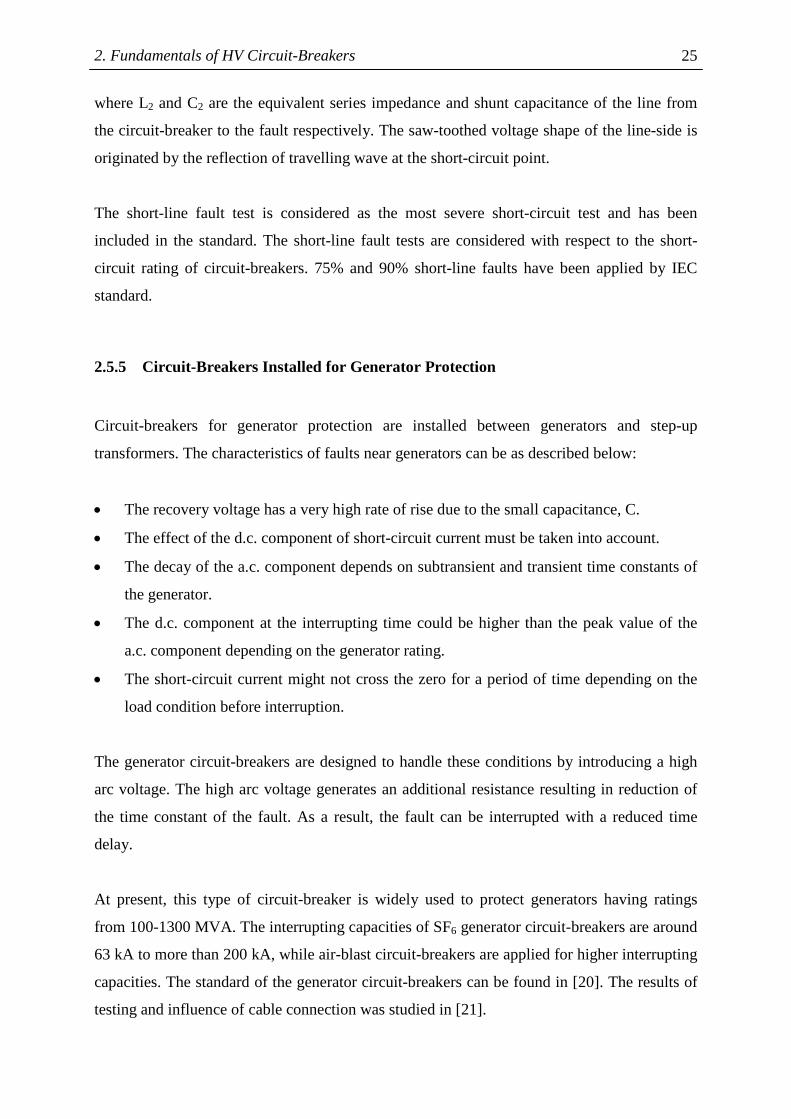
According to IEC standard, the characteristics of TRV can be determined by two methods:
two-parameter and four-parameter methods. These methods are based on the graphical
analysis which can represent the magnitude of TRV and RRRV. The two and four-parameter
methods are represented in Fig. 3.1 The detail of how to use these two methods to find the
magnitude of TRV and RRRV is represented in the appendix of [7].
(a) (b)
Figure 3.1: (a): two-parameter method, (b): four-parameter method
Normally, the two-parameter method is applied in systems with voltages less than 100 kV or
in systems with voltages greater than 100 kV where the short-circuit currents are relatively
small. In other cases, the four-parameter method is applied in systems with voltages 100 kV
and above. The TRV parameters in the IEC standard are classified with respect to proportion
of maximum short-circuit current rating, for example, 10 %, 30 %, 60 % and 100 %. The
characteristics of each test duty can be summarized as follows:
• 10% short-circuit current, IEC test duty 10: The fault current is supplied from only one
transformer and the TRV has very high steepness of 5.5 kV/µs at 100 kV to 12.6 kV/µs
at 765 kV.
• 30% short-circuit current, IEC test duty T30: The fault current is supplied from 1 or 2
transformers connected in parallel and the RRRV is 5 kV/µs for 100 kV and above.
• 60% short-circuit current, IEC test duty T60: The fault current is supplied from
transformers connected in parallel. The TRV has a steepness of 3 kV/µs for 100 kV and
above.
• 100% short-circuit current, IEC test duty T100: The RRRV is 2 kV/µs. The additional
requirement of this test duty is ability to interrupt short-circuit current with operating
sequence, for example, O-0.3s-CO-3min-CO. O represents opening operation and CO
3. Switching Stresses of HV Circuit-Breakers
33
represents closing operation followed immediately by an opening operation. The test
duty T100 can be divided into two types: T100s (test with symmetrical short-circuit
current) and T100a (test with asymmetrical short-circuit current).
3.2 Effects of Grounding and Types of Applications to Stresses of HV
Circuit-Breakers
In order to investigate electrical stresses of circuit-breakers according to effects of grounding
and types of applications, the 110 kV radial network model which has the short-circuit rating
of 40 kA and 10 kA is established. This model is composed of five transmission line circuits
and five cable circuits. The capacitor bank and the shunt reactor are also introduced in the
network to simulate the stresses of interruption of capacitive current and chopping current
respectively. Various types of grounding, isolated grounding, compensated grounding and
solid grounding, at the main transformer have been applied. Interrupted currents, TRV and
RRRV are taken into account in order to compare the stresses of circuit-breakers in any
applications. The simulation of TRV and RRRV have been carried out by using
PSCAD/EMTDC program, whereas short-circuit and load currents are simulated by
ABB/NEPLAN program.
3.2.1 Test System Configurations, Specifications and Modelling of Equipment
The test system diagram is represented in Fig. 3.2. The ratings of 380/110 kV transformers,
300 MVA and 1200 MVA, are selected regarding the rated short-circuit currents of 10 kA and
40 kA respectively. The specifications and modelling of elements can be represented as
follows:
• Voltage source: The voltage source of 380 kV with the rated short-circuit capacity of
63 kA is selected.
• 380/110 kV power transformers: The transformer ratings of 300 MVA and 1200 MVA
according to 10 kA and 40 kA respectively are applied. This 40 kA rating is considered
as the maximum short-circuit rating for 110 kV circuit-breakers.

3. Switching Stresses of HV Circuit-Breakers 34
• Transmission lines: The length of transmission line of 25 km/circuit is modelled as
distributed elements by using a frequency dependent model. The single conductor Al/St
240/40 and a double circuit have been used to model the transmission line circuit.
• 110 kV cables: The single conductor per phase of the XLPE cable with the length of
15 km/circuit has been used.
• 20 kV cables: The 20 kV cable with length of 80 km/circuit in the distribution network is
modelled as lumped shunt capacitance.
• 110/20 kV distribution transformers: The distribution transformers of 31.5 MVA are
selected for supplying the loads of 13.5 MW/circuit.
• Shunt reactor: The shunt reactor of 100 MVar is installed at the receiving end of the 110
kV cable circuit to compensate the reactive power. Stray capacitance with the natural
frequency of 2 kHz must be taken into account.
• Capacitor banks: Grounded and ungrounded capacitor banks of 10 MVar are installed
behind the main circuit-breaker in order to study the stresses between different
configurations.
• Load: In each circuit, the load of 15 MVA at 0.9 power factor is taken into consideration.
The load model for medium voltage system is recommended in [30]. The parallel
capacitance represents the capacitance of cable in distribution circuit.
• System groundings: The groundings of the system are composed of three types: isolated,
compensated and solid grounding. The compensating coil in compensated grounding is
introduced in order to compensate the earthed fault current.
3.2.2 Simulation Cases
Different circuit-breaker applications have been introduced in order to simulate stresses of
circuit-breakers. In every application, the simulation is carried out by changing types of
grounding and interrupting currents. The three main parameters: interrupted current, TRV and
RRRV are taken into account. The applications of circuit-breakers in this study are composed
of:
1. Switching-off no-load transmission line (Fig. 3.3a)
2. Switching-off no-load cable (Fig. 3.3b)
3. Interruption of single-phase 90 % short-line fault in transmission line (Fig. 3.3c)
3. Switching Stresses of HV Circuit-Breakers
35
1200MVA or 300MVA380/110 kV
ukr=15%
31.5MVA110/20kV
ukr=15%,uv=0.5%
Y
Y25km
CR
XS(f)Xp(f)
31.5MVA110/20kV
ukr=15%,uv=0.5%
Y
CR
XS(f)Xp(f)
Transmission line, Double-circuit
15km
Cable (Al), 500 mm2, XLPE-Isolation
X5
X5
15 MVA0,9 power factor
15 MVA0,9 power factor
Reactor100 MVar
Figure 3.2: Simulation diagram of a test radial 110 kV system
4. Interruption of three-phase 90 % short-line fault in transmission line (Fig. 3.3d)
5. Interruption of single-phase 90 % short-line fault in cable (Fig. 3.3e)
6. Interruption of three-phase 90 % short-line fault in cable (Fig. 3.3f)
7. Switching-off ungrounded capacitor bank (Fig. 3.3g)
8. Switching-off grounded capacitor bank (Fig. 3.3h)
9. Switching-off shunt reactor (chopping current of 2.5 A, Fig. 3.3i)
TRV waveforms of the first-phase-to-clear of HV circuit-breakers in mentioned applications
are illustrated in Fig. 3.3
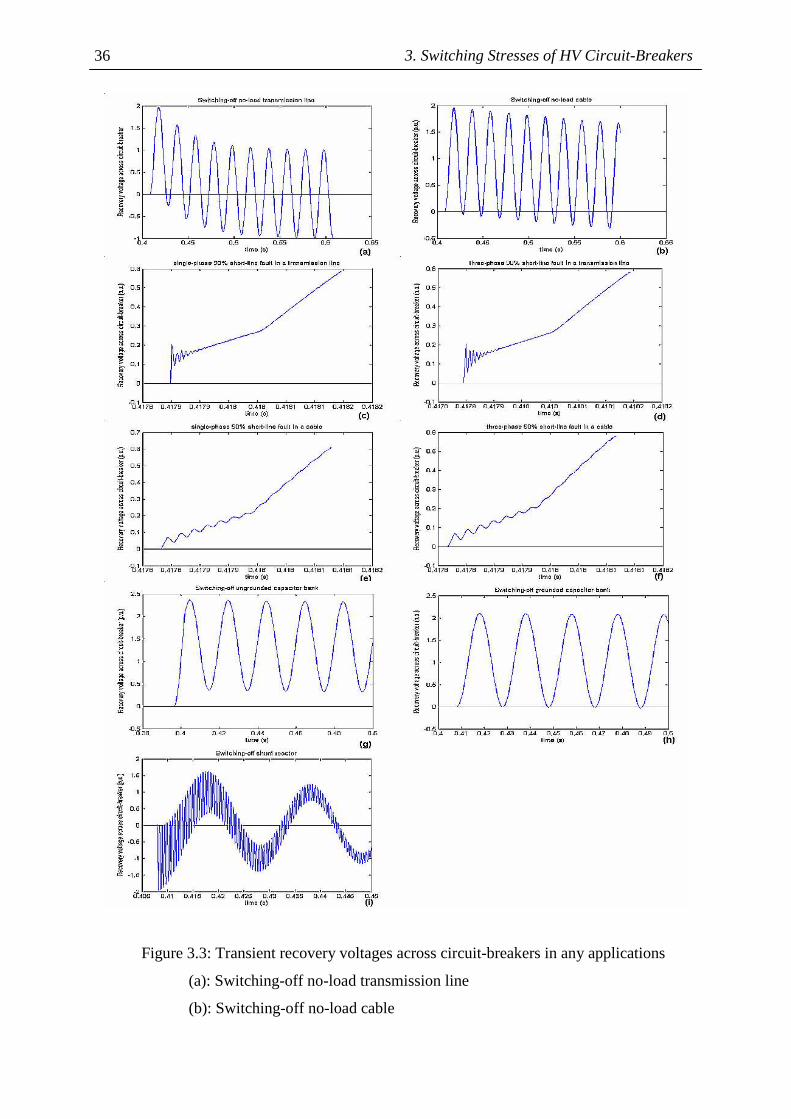
3. Switching Stresses of HV Circuit-Breakers 36
Figure 3.3: Transient recovery voltages across circuit-breakers in any applications
(a): Switching-off no-load transmission line
(b): Switching-off no-load cable

3. Switching Stresses of HV Circuit-Breakers
37
(c): Interruption of single-phase 90 % short-line fault in transmission line
(d): Interruption of three-phase 90 % short-line fault in transmission line
(e): Interruption of single-phase 90 % short-line fault in cable
(f): Interruption of three-phase 90 % short-line fault in cable
(g): Switching-off ungrounded capacitor bank
(h): Switching-off grounded capacitor bank
(i): Switching-off shunt reactor
3.2.3 Simulation Conditions
In order to simulate transients in power systems, the conditions of the simulation must be paid
attention, for example, the simulation time step and applied models. The simulation
conditions in this study are described as follows:
• Simulation time step: The simulation time step is determined by the maximum expected
frequency (maxf ) which is recommended in [30]. The simulation time step can be
determined from:
max
1∆t
10×f≤ (3.1)
The simulation time step of 1 µs is applied for the simulation cases of short-line faults
(cases 3-6), since the maximum expected frequency of the beginning of the recovery
voltage is very high. The time step of 5 µs is applied for the case 9, whereas the time step
of 50 µs is sufficient for cases 1, 2, 7 and 8.
• Opening of circuit-breaker: Circuit-breakers are requested to open at current zero in
cases 1-8 and at 2.5 A in case 9. The opening time after the initiation of faults is not less
than 100 ms.
• System grounding point: In case of isolated grounding, there are no grounding points at
any transformers. The grounding point in cases of compensated and solid grounding is
employed at the 380/110 kV main transformer.
• Transmission lines and cable models: The configurations, for example, conductor
configuration, tower configuration, sag distance and insulation configuration must be
taken into account.
3. Switching Stresses of HV Circuit-Breakers 38
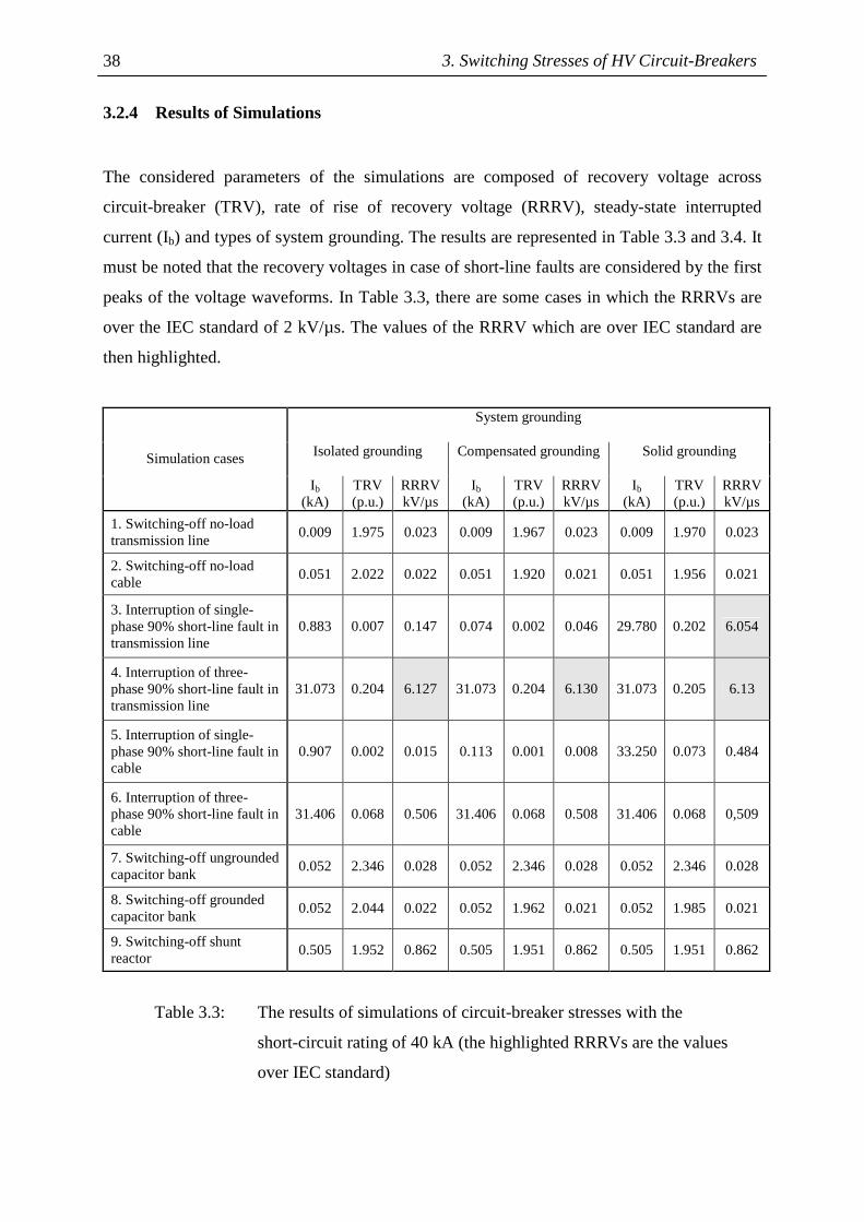
3.2.4 Results of Simulations
The considered parameters of the simulations are composed of recovery voltage across
circuit-breaker (TRV), rate of rise of recovery voltage (RRRV), steady-state interrupted
current (Ib) and types of system grounding. The results are represented in Table 3.3 and 3.4. It
must be noted that the recovery voltages in case of short-line faults are considered by the first
peaks of the voltage waveforms. In Table 3.3, there are some cases in which the RRRVs are
over the IEC standard of 2 kV/µs. The values of the RRRV which are over IEC standard are
then highlighted.
System grounding
Isolated grounding
Compensated grounding Solid grounding Simulation cases
Ib (kA)
TRV (p.u.)
RRRV kV/µs
Ib (kA)
TRV
(p.u.) RRRV kV/µs
Ib (kA)
TRV
(p.u.) RRRV kV/µs
1. Switching-off no-load transmission line
0.009 1.975 0.023 0.009 1.967 0.023 0.009 1.970 0.023
2. Switching-off no-load cable
0.051 2.022 0.022 0.051 1.920 0.021 0.051 1.956 0.021
3. Interruption of single-phase 90% short-line fault in transmission line
0.883 0.007 0.147 0.074 0.002 0.046 29.780 0.202 6.054
4. Interruption of three-phase 90% short-line fault in transmission line
31.073 0.204 6.127 31.073 0.204 6.130 31.073 0.205 6.13
5. Interruption of single-phase 90% short-line fault in cable
0.907 0.002 0.015 0.113 0.001 0.008 33.250 0.073 0.484
6. Interruption of three-phase 90% short-line fault in cable
31.406 0.068 0.506 31.406 0.068 0.508 31.406 0.068 0,509
7. Switching-off ungrounded capacitor bank
0.052 2.346 0.028 0.052 2.346 0.028 0.052 2.346 0.028
8. Switching-off grounded capacitor bank
0.052 2.044 0.022 0.052 1.962 0.021 0.052 1.985 0.021
9. Switching-off shunt reactor
0.505 1.952 0.862 0.505 1.951 0.862 0.505 1.951 0.862
Table 3.3: The results of simulations of circuit-breaker stresses with the
short-circuit rating of 40 kA (the highlighted RRRVs are the values
over IEC standard)
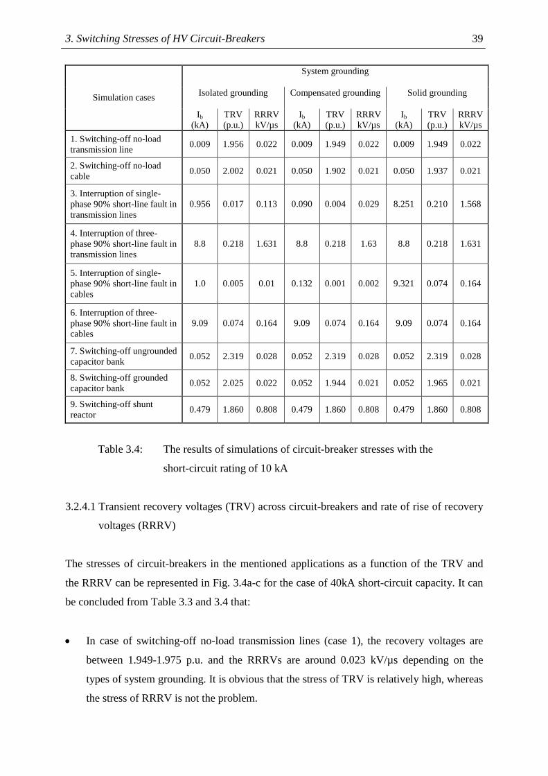
3. Switching Stresses of HV Circuit-Breakers
39
System grounding
Isolated grounding
Compensated grounding Solid grounding Simulation cases
Ib (kA)
TRV (p.u.)
RRRV kV/µs
Ib (kA)
TRV
(p.u.) RRRV kV/µs
Ib (kA)
TRV
(p.u.) RRRV kV/µs
1. Switching-off no-load transmission line
0.009 1.956 0.022 0.009 1.949 0.022 0.009 1.949 0.022
2. Switching-off no-load cable
0.050 2.002 0.021 0.050 1.902 0.021 0.050 1.937 0.021
3. Interruption of single-phase 90% short-line fault in transmission lines
0.956 0.017 0.113 0.090 0.004 0.029 8.251 0.210 1.568
4. Interruption of three-phase 90% short-line fault in transmission lines
8.8 0.218 1.631 8.8 0.218 1.63 8.8 0.218 1.631
5. Interruption of single-phase 90% short-line fault in cables
1.0 0.005 0.01 0.132 0.001 0.002 9.321 0.074 0.164
6. Interruption of three-phase 90% short-line fault in cables
9.09 0.074 0.164 9.09 0.074 0.164 9.09 0.074 0.164
7. Switching-off ungrounded capacitor bank
0.052 2.319 0.028 0.052 2.319 0.028 0.052 2.319 0.028
8. Switching-off grounded capacitor bank
0.052 2.025 0.022 0.052 1.944 0.021 0.052 1.965 0.021
9. Switching-off shunt reactor
0.479 1.860 0.808 0.479 1.860 0.808 0.479 1.860 0.808
Table 3.4: The results of simulations of circuit-breaker stresses with the
short-circuit rating of 10 kA
3.2.4.1 Transient recovery voltages (TRV) across circuit-breakers and rate of rise of recovery
voltages (RRRV)
The stresses of circuit-breakers in the mentioned applications as a function of the TRV and
the RRRV can be represented in Fig. 3.4a-c for the case of 40kA short-circuit capacity. It can
be concluded from Table 3.3 and 3.4 that:
• In case of switching-off no-load transmission lines (case 1), the recovery voltages are
between 1.949-1.975 p.u. and the RRRVs are around 0.023 kV/µs depending on the
types of system grounding. It is obvious that the stress of TRV is relatively high, whereas
the stress of RRRV is not the problem.

3. Switching Stresses of HV Circuit-Breakers 40
• The TRVs and the RRRVs in case of switching-off no-load cables (case 2) are 1.902-
2.002 p.u. and 0.022 kV/µs respectively. In comparison to switching-off transmission
lines, the stress of the TRV is slightly higher in the case of isolated system grounding,
but the stress of the RRRV is fairly similar.
• The results from the short-line fault in transmission lines show that the RRRVs relate to
the interrupted currents and characteristic impedances. It can be seen that the RRRVs in
the case of single-phase short-line fault (case 3) with isolating grounding and
compensated grounding are relatively low compared with the case of solid grounding and
3-phase short-line fault (case 4).
• The stresses of the RRRVs in case of short-line fault in cables are not so severe as in the
case of the short-line fault in transmission lines because of the lower characteristic
impedances of the cables. The RRRVs of single-phase and 3-phase short-line faults are
not higher than 0.51 kV/µs.
• Switching-off ungrounded capacitor banks results in the highest TRVs (~2.3-2.35 p.u.)
regardless of the types of system grounding. The stresses of RRRVs can be neglected due
to very low RRRVs.
• The TRVs in the case of switching-off grounded capacitor banks lie between 1.94 p.u.
and 2.04 p.u. corresponding to the system grounding and rating. It is shown that the
TRVs are slightly higher when the ratings of the systems are higher. The stresses of the
RRRVs play no important roles in this case.
• The stresses of switching-off the shunt reactor from the TRVs and RRRVs are
moderately high. The TRVs are around 1.86-1.95 p.u. and the RRRVs are around 0.808-
0.862 kV/µs.
0 0.2 0.4 0.6 0.8 1 1.2 1.4 1.6 1.8 20
0.2
0.4
0.6
0.8
1
1.2
1.4
1.6
1.8
2
2.2
2.4
Rate of Rise of Recovery Voltage (kV/µs)
Tra
nsi
en
t re
cov
ery
vol
tage
(p.
u.)
1
3
2 98
7
4
5 6 (6.13,0.2)
(a)

3. Switching Stresses of HV Circuit-Breakers
41
0 0.2 0.4 0.6 0.8 1 1.2 1.4 1.6 1.8 20
0.2
0.4
0.6
0.8
1
1.2
1.4
1.6
1.8
2
2.2
2.4
Rate of Rise of Recovery Voltage (kV/µs)
Tra
nsie
nt R
eco
very
Vo
ltag
e (p
.u.)
7
82
19
35 6
4(6.13,0.2)
(b)
0 0.2 0.4 0.6 0.8 1 1.2 1.4 1.6 1.8 2 0
0.2
0.4
0.6
0.8
1
1.2
1.4
1.6
1.8
2
2.2
2.4
Rate of Rise of Recovery Voltage (kV/µs)
Tra
nsie
nt R
ecov
ery
Vol
tage
(p
.u.)
7
8
21 9
35 6
4(6.13,0.2) (6.05,0.2)
(c)
Figure. 3.4: Transient recovery voltages (TRVs) and rate of rise of recovery
voltages (RRRVs) of different applications
(a): Isolated grounding system
(b): Compensated grounding system
(c): Solidly grounded system
3.2.4.2 Interrupted currents and rate of rise of recovery voltages (RRRVs)
The relationship between interrupted currents and the RRRVs can be depicted in Fig. 3.5a and
b. It can be concluded that:
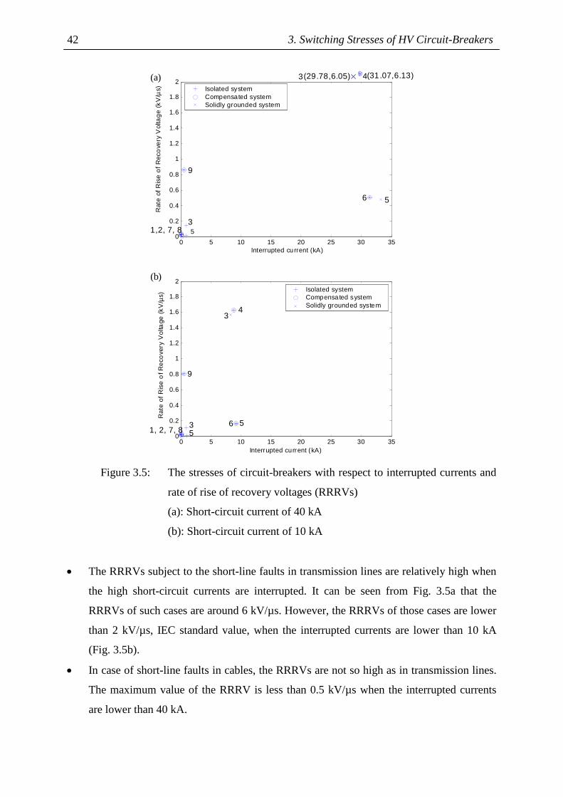
3. Switching Stresses of HV Circuit-Breakers 42
0 5 10 15 20 25 30 350
0.2
0.4
0.6
0.8
1
1.2
1.4
1.6
1.8
2Isolated systemCompensated systemSolidly grounded system
1,2, 7, 8
9
3
5 6
4
Interrupted current (kA)
Rat
e of
Ris
e o
f R
eco
very
Vol
tag
e (k
V/µ
s)
3 (31 .07,6.13) (29.78,6.05)
5
(a)
0 5 10 15 20 25 30 350
0.2
0.4
0.6
0.8
1
1.2
1.4
1.6
1.8
2
Interrupted current (kA)
Rat
e of
Ris
e o
f Rec
ove
ry V
olta
ge (
kV/µ
s)
Isolated systemCompensated systemSolidly grounded system
3 4
9
3 5 1, 2, 7, 8
6 5
(b)
Figure 3.5: The stresses of circuit-breakers with respect to interrupted currents and
rate of rise of recovery voltages (RRRVs)
(a): Short-circuit current of 40 kA
(b): Short-circuit current of 10 kA
• The RRRVs subject to the short-line faults in transmission lines are relatively high when
the high short-circuit currents are interrupted. It can be seen from Fig. 3.5a that the
RRRVs of such cases are around 6 kV/µs. However, the RRRVs of those cases are lower
than 2 kV/µs, IEC standard value, when the interrupted currents are lower than 10 kA
(Fig. 3.5b).
• In case of short-line faults in cables, the RRRVs are not so high as in transmission lines.
The maximum value of the RRRV is less than 0.5 kV/µs when the interrupted currents
are lower than 40 kA.

3. Switching Stresses of HV Circuit-Breakers
43
• Stresses of circuit-breakers in terms of the RRRVs in other cases are not so severe
because they are lower than standard value of 2 kV/µs
3.2.5 Conclusions
Stresses of circuit-breakers in terms of the TRVs, the RRRVs and interrupted currents can be
concluded from the simulations:
• Types of system grounding result in different TRVs, RRRVs and interrupted currents.
For example, the interrupted currents of single-phase short-line faults are relatively low
in case of isolated grounding and compensated grounding compared with solid
grounding. However, types of grounding play no important role in case of 3-phase short-
line faults and switching-off ungrounded capacitor banks.
• In the case of capacitive switching (except switching ungrounded capacitor banks), the
TRVs in an isolated system are higher than those in a solidly grounded system and a
compensated system respectively. These TRVs are dependent of the ratio of positive-
sequence to zero-sequence capacitance (C1/C0).
• The interrupted currents of single-phase short line faults in a solidly grounded system are
relatively high since the faults occur near the supply. In real distribution system, they
would not be so high because of the impedances from the power plant to the faulted
position are taken into account. Nevertheless, single-phase short line faults must be
considered when the circuit-breakers are installed near power plants.
• It is obvious that 3-phase short-line faults result in very high RRRVs thus leading to the
breakdown of circuit-breakers. In order to reduce the very high RRRVs, the resistance or
capacitance will be applied in parallel with contact break.
• It could be concluded from the simulation that the circuit-breakers designed for
interrupting capacitor banks can be also used for interrupting no-load transmission lines
and no-load cables.
• It is evident that the RRRVs in case of short-line faults are related to the interrupted
currents.
• The configuration of the whole system plays an important role in the TRVs and the
RRRVs. For example, the zero-sequence capacitances of cable circuits affect the
3. Switching Stresses of HV Circuit-Breakers 44
transient recovery voltages. Without these cable circuits, transient recovery voltages are
supposed to be higher.
• In comparison to IEC standard, the values of the RRRV in most cases are lower than the
standard value (2 kV/µs) except in some cases of interruption due to a short-line fault in a
cable and/or transmission line.
3.3 Stresses of HV Circuit-Breakers by Combined Statistical Method
The electrical stresses of circuit-breakers are mainly determined by operating currents, short-
circuit currents and switching operation. In addition, the number of faults on overhead lines
which circuit-breakers have to be interrupted is taken into account but considered separately
from the electrical stresses. The aim of this study is to combine and investigate electrical
stresses of circuit-breakers as a function of fault frequency and fault severity. The
combination of fault density and fault severity of circuit-breakers are carried out by statistical
method. Number of faults, short-circuit currents and length of transmission lines in 123 kV,
245 kV and 420 kV were collected from the utility during 10-year operation.
3.3.1 Concepts of Combined Statistical Method
The approach of combined statistical method is introduced by [31] and is mentioned as
Chessboard method. This method can combine stresses of circuit-breakers as a function of
fault density and fault severity. The result of the investigation indicates which areas are
subject to the highest stress and which area the faults most frequently take place.
3.3.2 Investigation of HV Circuit-breaker Database
The population of circuit-breakers is taken from a utility in Germany. Only this utility is taken
into account, since the utility provides the required information, such as number of faults,
short-circuit currents and the length of transmission lines. Such information is necessary for
the combined statistical method. Due to lack of complete information, other databases from
other utilities cannot be applied in this study. The total population of circuit-breakers on
different voltage levels is represented in Table 3.5.
3. Switching Stresses of HV Circuit-Breakers
45
123 kV 245 kV 420 kV
no. of circuit-breakers 656 74 55
Table 3.5: The total population of HV circuit-breakers
Transmission lines in 123 kV, 245 kV and 420 kV are taken into consideration. However, not
every transmission is subject to the faults. Table 3.6 represents the total number of
transmission lines and the total lengths. It can be calculated from Table 3.6 that the
proportions of faults in terms of the line length are 28.84 %, 66.33 % and 84.94 % in 123 kV,
245 kV and 420 kV respectively. In comparison with the proportions of faults (in terms of
number of faulted lines), the proportions of faults are 22.40 %, 45.24 % and 48.39 % in
123 kV, 245 kV and 420 kV respectively. In conclusion, the faulted areas in higher voltage
levels are larger than in lower voltage levels.
123 kV 245 kV 420 kV
no. of lines 299 42 31
the length of lines (km) 3320 1417 963
no. of faulted lines 67 19 15
the length of faulted lines 951 940 818
Table 3.6: The population of transmission lines and the lengths of transmission lines
The maximum expected short-circuit currents in the substations had been recorded and
divided by the rated short-circuit breaking currents (Irb). Regardless of fault types, faults of
each phase on faulted transmission lines were investigated. The numbers of faults per phase
on different voltage levels are represented in Table 3.7
123 kV 245 kV 420 kV
no. of faults per phase 352 307 260
Table 3.7: Investigated faults on transmission lines
In connection with Table 3.6, the average number of faults per phase per line on different
voltage levels can be calculated. It is represented that the average number of faults per phase
3. Switching Stresses of HV Circuit-Breakers 46
per line are 5.25, 16.16 and 17.33 in 123 kV, 245 kV and 245 kV respectively. It is obvious
that the higher the voltage level, the higher the numbers of faults per phase per line.
3.3.3 Data Evaluation and Analysis
In order to apply the combined statistical method, the necessary information is collected and
then investigated. The data evaluation steps are represented in Fig.3.6
Transmission line length and maximum expected Isc are taken into account
Every fault per phase on transmission lines is normalized on 100 km basis
Percentile of fault per phase per 100 km is calculated
Percentile of Isc/Irb is calculated
Combined statistical method is applied
Figure 3.6: Steps of evaluation
The density of fault or frequency of fault can be calculated by using transmission line length
and numbers of faults. After that the values are normalized on a 100 km basis. Every fault in
every transmission line is separately considered. In other words, “faults per phase per 100
km” of each fault can be calculated by the following equation.
Faults per phase per 100 km = (1/line length) x 100 (3.2)
The examples of fault determination from the database are given in Table 3.8. After faults per
phase per 100 km are calculated, the percentile of them are then determined. Fault severity or

3. Switching Stresses of HV Circuit-Breakers
47
the proportion of maximum expected short-circuit current to rated breaking current (Isc/Irb)
can be obtained from the database. Afterwards, the percentile of it is determined
fault ID Line length (km) Faults/phase/100 km Isc/Irb
1 4.5 22.22 0.71
2 4.5 22.22 0.71
3 10.4 9.62 0.53
4 10.4 9.62 0.53
5 10.4 9.62 0.53
6 10.4 9.62 0.53
7 17.5 5.72 0.23
8 17.5 5.72 0.23
9 17.5 5.72 0.23
10 23.02 4.34 0.31
Table 3.8: The examples of fault determination
3.3.4 Implementation of Combined Statistical Method
The percentiles of faults per phase per 100 km and percentiles of Isc/Irb in 123 kV, 245 kV and
420 kV are carried out. Table 3.9 represents the percentiles of faults per phase per 100 km and
percentiles of Isc/Irb. In 245 kV and 420 kV, there are only 19 and 15 faulted transmission
lines respectively, thus resulting in repetitive “faults per phase per 100 km” values. As a
result, the percentiles in 245 kV and 420 kV are not well distributed.
The percentiles of faults per phase per 100 km and percentiles of Isc/Irb can be represented in
terms of graphs as shown in Fig. 3.7 and 3.8
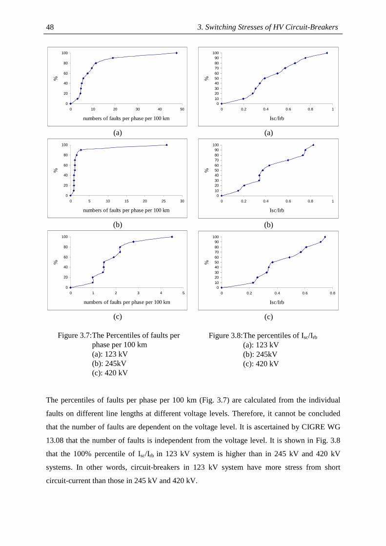
3. Switching Stresses of HV Circuit-Breakers 48
0
20
40
60
80
100
0 10 20 30 40 50
numbers of faults per phase per 100 km
%
(a)
0
20
40
60
80
100
0 5 10 15 20 25 30
numbers of faults per phase per 100 km
%
(b)
0
20
40
60
80
100
0 1 2 3 4 5
numbers of faults per phase per 100 km
%
(c)
Figure 3.7: The Percentiles of faults per phase per 100 km (a): 123 kV (b): 245kV (c): 420 kV
0102030405060708090
100
0 0.2 0.4 0.6 0.8 1
Isc/Irb
%
(a)
0102030405060708090
100
0 0.2 0.4 0.6 0.8 1
Isc/Irb%
(b)
0102030405060708090
100
0 0.2 0.4 0.6 0.8
Isc/Irb
%
(c)
Figure 3.8: The percentiles of Isc/Irb
(a): 123 kV (b): 245kV
(c): 420 kV
The percentiles of faults per phase per 100 km (Fig. 3.7) are calculated from the individual
faults on different line lengths at different voltage levels. Therefore, it cannot be concluded
that the number of faults are dependent on the voltage level. It is ascertained by CIGRE WG
13.08 that the number of faults is independent from the voltage level. It is shown in Fig. 3.8
that the 100% percentile of Isc/Irb in 123 kV system is higher than in 245 kV and 420 kV
systems. In other words, circuit-breakers in 123 kV system have more stress from short
circuit-current than those in 245 kV and 420 kV.
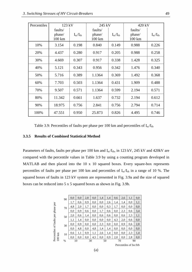
3. Switching Stresses of HV Circuit-Breakers
49
Percentiles 123 kV 245 kV 420 kV
faults/ phase/ 100 km
Isc/Irb
faults/ phase/ 100 km
Isc/Irb
faults/ phase/ 100 km
Isc/Irb
10% 3.154 0.198 0.840 0.149 0.988 0.226
20% 4.437 0.280 0.917 0.205 0.988 0.258
30% 4.669 0.307 0.917 0.338 1.428 0.325
40% 5.121 0.343 0.956 0.342 1.476 0.340
50% 5.716 0.389 1.1364 0.369 1.492 0.368
60% 7.703 0.503 1.1364 0.431 1.909 0.488
70% 9.507 0.571 1.1364 0.599 2.194 0.571
80% 11.342 0.661 1.637 0.732 2.194 0.612
90% 18.975 0.756 2.841 0.756 2.794 0.714
100% 47.551 0.950 25.873 0.826 4.495 0.746
Table 3.9: Percentiles of faults per phase per 100 km and percentiles of Isc/Irb
3.3.5 Results of Combined Statistical Method
Parameters of faults, faults per phase per 100 km and Isc/Irb, in 123 kV, 245 kV and 420kV are
compared with the percentile values in Table 3.9 by using a counting program developed in
MATLAB and then placed into the 10 x 10 squared boxes. Every square-box represents
percentiles of faults per phase per 100 km and percentiles of Isc/Irb in a range of 10 %. The
squared boxes of faults in 123 kV system are represented in Fig. 3.9a and the size of squared
boxes can be reduced into 5 x 5 squared boxes as shown in Fig. 3.9b.
0,0 0,0 2,8 0,0 1,4 1,4 0,6 2,6 1,1 0,0 90 1,7 0,6 0,9 0,0 0,0 2,6 1,4 1,4 0,0 1,1
4,8 2,0 1,7 0,0 0,0 0,3 1,7 0,0 0,0 0,0 70 0,0 0,9 0,6 0,0 1,7 0,6 0,0 2,3 0,6 3,4
2,0 0,6 1,4 0,0 0,6 0,6 0,0 0,6 2,3 1,1 50 1,1 1,4 0,0 0,0 0,0 0,0 4,3 2,0 0,6 0,0
0,0 0,9 0,0 0,0 2,3 0,0 0,0 0,9 0,6 2,8 30 0,0 4,8 0,0 4,8 1,4 1,4 0,0 0,0 0,0 0,0
0,6 1,1 0,9 1,1 2,6 1,4 0,0 0,0 2,3 1,4 10 0,0 0,0 0,0 4,5 0,0 0,9 2,0 0,0 2,8 0,0
Per
cen
tiles
of
fau
lts p
er p
has
e p
er
10
0 km
% 10 30 50 70 90
Percentiles of Isc/Irb
(a)
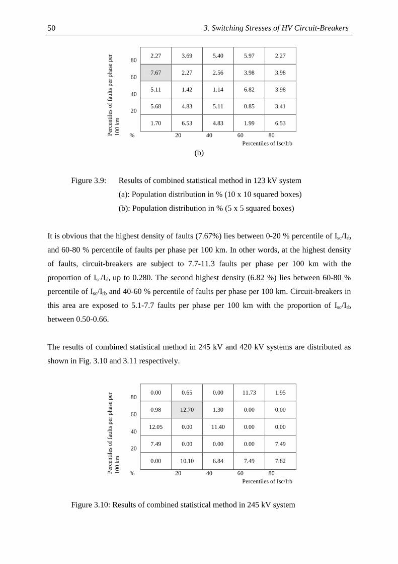
3. Switching Stresses of HV Circuit-Breakers 50
80 2.27 3.69 5.40 5.97 2.27
60 7.67 2.27 2.56 3.98 3.98
40 5.11 1.42 1.14 6.82 3.98
20 5.68 4.83 5.11 0.85 3.41
1.70 6.53 4.83 1.99 6.53
Per
cen
tiles
of
fau
lts p
er p
has
e p
er
10
0 km
% 20 40 60 80 Percentiles of Isc/Irb
(b)
Figure 3.9: Results of combined statistical method in 123 kV system
(a): Population distribution in % (10 x 10 squared boxes)
(b): Population distribution in % (5 x 5 squared boxes)
It is obvious that the highest density of faults (7.67%) lies between 0-20 % percentile of Isc/Irb
and 60-80 % percentile of faults per phase per 100 km. In other words, at the highest density
of faults, circuit-breakers are subject to 7.7-11.3 faults per phase per 100 km with the
proportion of Isc/Irb up to 0.280. The second highest density (6.82 %) lies between 60-80 %
percentile of Isc/Irb and 40-60 % percentile of faults per phase per 100 km. Circuit-breakers in
this area are exposed to 5.1-7.7 faults per phase per 100 km with the proportion of Isc/Irb
between 0.50-0.66.
The results of combined statistical method in 245 kV and 420 kV systems are distributed as
shown in Fig. 3.10 and 3.11 respectively.
80 0.00 0.65 0.00 11.73 1.95
60 0.98 12.70 1.30 0.00 0.00
40 12.05 0.00 11.40 0.00 0.00
20 7.49 0.00 0.00 0.00 7.49
0.00 10.10 6.84 7.49 7.82
Per
cen
tiles
of
fau
lts p
er p
has
e p
er
10
0 km
% 20 40 60 80 Percentiles of Isc/Irb
Figure 3.10: Results of combined statistical method in 245 kV system
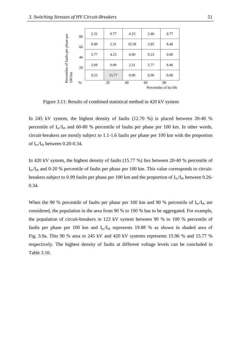
3. Switching Stresses of HV Circuit-Breakers
51
80 2.31 0.77 4.23 3.46 0.77
60 0.00 2.31 10.38 3.85 8.46
40 5.77 4.23 0.00 9.23 0.00
20 2.69 0.00 2.31 5.77 8.46
9.23 15.77 0.00 0.00 0.00
Per
cen
tiles
of
fau
lts p
er p
has
e p
er
10
0 km
% 20 40 60 80 Percentiles of Isc/Irb
Figure 3.11: Results of combined statistical method in 420 kV system
In 245 kV system, the highest density of faults (12.70 %) is placed between 20-40 %
percentile of Isc/Irb and 60-80 % percentile of faults per phase per 100 km. In other words,
circuit-breakers are mostly subject to 1.1-1.6 faults per phase per 100 km with the proportion
of Isc/Irb between 0.20-0.34.
In 420 kV system, the highest density of faults (15.77 %) lies between 20-40 % percentile of
Isc/Irb and 0-20 % percentile of faults per phase per 100 km. This value corresponds to circuit-
breakers subject to 0.99 faults per phase per 100 km and the proportion of Isc/Irb between 0.26-
0.34.
When the 90 % percentile of faults per phase per 100 km and 90 % percentile of Isc/Irb are
considered, the population in the area from 90 % to 100 % has to be aggregated. For example,
the population of circuit-breakers in 123 kV system between 90 % to 100 % percentile of
faults per phase per 100 km and Isc/Irb represents 19.88 % as shown in shaded area of
Fig. 3.9a. This 90 % area in 245 kV and 420 kV systems represents 15.96 % and 15.77 %
respectively. The highest density of faults at different voltage levels can be concluded in
Table 3.10.
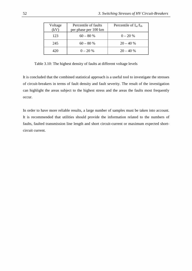
3. Switching Stresses of HV Circuit-Breakers 52
Voltage (kV)
Percentile of faults per phase per 100 km
Percentile of Isc/Irb
123 60 – 80 % 0 – 20 %
245 60 – 80 % 20 – 40 %
420 0 – 20 % 20 – 40 %
Table 3.10: The highest density of faults at different voltage levels
It is concluded that the combined statistical approach is a useful tool to investigate the stresses
of circuit-breakers in terms of fault density and fault severity. The result of the investigation
can highlight the areas subject to the highest stress and the areas the faults most frequently
occur.
In order to have more reliable results, a large number of samples must be taken into account.
It is recommended that utilities should provide the information related to the numbers of
faults, faulted transmission line length and short circuit-current or maximum expected short-
circuit current.

4. Failure Modes and Effects Analysis 53
4 Failure Modes and Effects Analysis
4.1 Concepts and Definitions
The main principles of designing optimal diagnosis and maintenance programs depend on the
basis of: which types and how often the failures occur, how severe the consequences are and
which maintenance strategies are suitable to prevent such failures. Failure Modes and Effects
Analysis (FMEA) is the systematic approach to investigate failures by identifying functions,
failure modes and consequences of failures. In addition, the failure database such as the
probability of failures must be integrated into the FMEA approach in order to assess the
severity of failures.
FMEA can be considered as an important part of Reliability-Centred Maintenance (RCM)
which is the method for achieving cost-effective programs. RCM was first applied in the civil
aircraft industry in 1960s for the Boeing 747 series, which are more complicated than
previous types. Concepts and fundamental principles of RCM can be defined in [32], [33] and
[34]. It can be concluded from the first definition of RCM [33] that the aims of RCM method
are: preservation of system functions, identification of failure modes, prioritizing of functions
and selection of effective maintenance programs. The other definition and process of RCM
method are based on seven questions [34]:
• What are the functions and associated performance standards?
• In what ways can the functions fail?
• What are the causes of each functional failure?
• What are the effects of each failure?
• What are the consequences of each failure?
• How to predict or prevent each failure?
• What can be done if there is no suitable preventive task?

4. Failure Modes and Effects Analysis 54
The steps of an RCM analysis can be summarized as followed [35]:
• Study preparation
• System selection and definition
• Functional failure analysis
• Critical item selection
• Data collection and analysis
• Failure modes and effects analysis
• Selection of maintenance tasks
• Determination of maintenance intervals
• Preventive maintenance comparison analysis
• Treatment of non-critical items
The application of RCM to power systems was first introduced by EPRI in the area of the
nuclear power industry. In the area of substation and HV circuit-breakers, the RCM methods
and techniques can be reviewed in [36], [37] and [38]. The more detail and complete process
of RCM applied to distribution systems is shown in [39]. In that study, the cable systems were
selected from the RCM process to perform maintenance evaluation.
In the following evaluation, the application of FMEA to HV circuit-breakers had been studied
and implemented in two aspects:
• Which components affect the functional failures of circuit-breakers
• How high are the risks to components in circuit-breakers
In order to conduct a FMEA process for HV circuit-breakers, the functions of circuit-breakers
must be first defined. Afterwards, the types of damages from the functional failures are listed.
The consequences of failures are then investigated by considering four main categories of
consequences: personnel safety, environmental impact, operation availability and costs of
repair. With the integration of the HV circuit-breaker database of Darmstadt University of
Technology, it is possible to evaluate the severity of failures of each component of circuit-
breakers resulting in risk assessment.
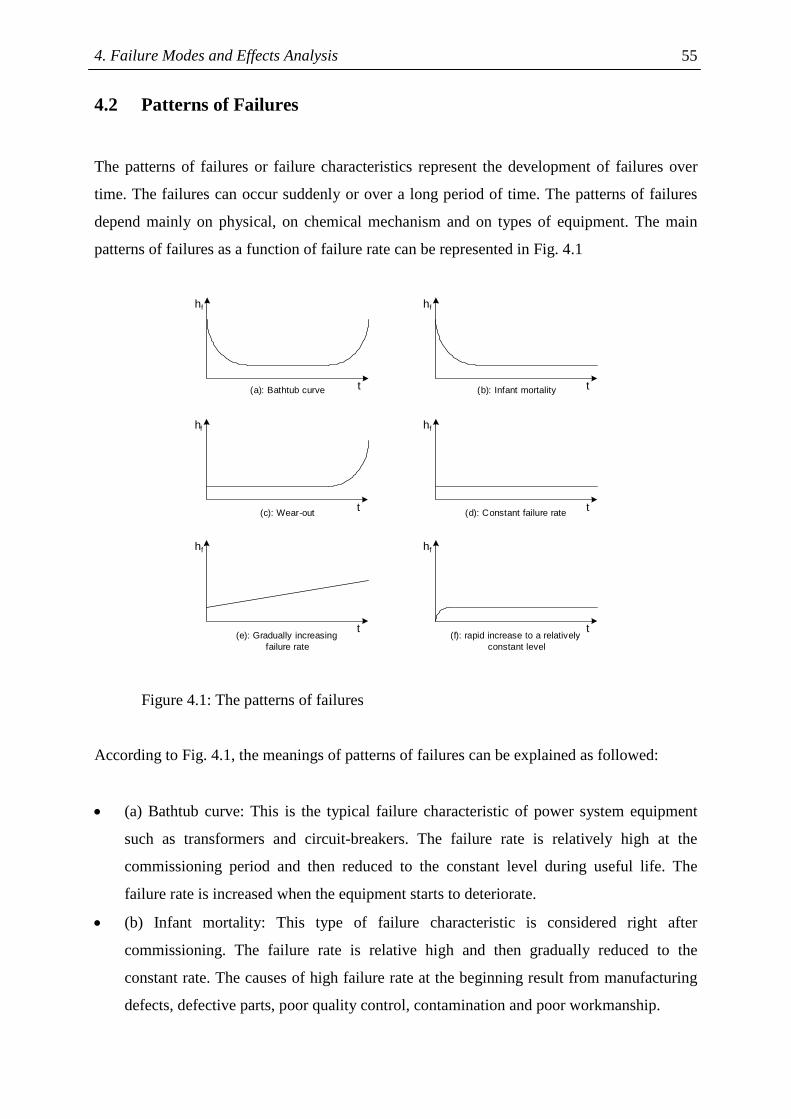
4. Failure Modes and Effects Analysis 55
4.2 Patterns of Failures
The patterns of failures or failure characteristics represent the development of failures over
time. The failures can occur suddenly or over a long period of time. The patterns of failures
depend mainly on physical, on chemical mechanism and on types of equipment. The main
patterns of failures as a function of failure rate can be represented in Fig. 4.1
hf
t
hf
t
hf
t
hf
t
hf
t
hf
t
(a): Bathtub curve (b): Infant mortality
(c): Wear-out (d): Constant failure rate
(e): Gradually increasingfailure rate
(f): rapid increase to a relatively constant level
Figure 4.1: The patterns of failures
According to Fig. 4.1, the meanings of patterns of failures can be explained as followed:
• (a) Bathtub curve: This is the typical failure characteristic of power system equipment
such as transformers and circuit-breakers. The failure rate is relatively high at the
commissioning period and then reduced to the constant level during useful life. The
failure rate is increased when the equipment starts to deteriorate.
• (b) Infant mortality: This type of failure characteristic is considered right after
commissioning. The failure rate is relative high and then gradually reduced to the
constant rate. The causes of high failure rate at the beginning result from manufacturing
defects, defective parts, poor quality control, contamination and poor workmanship.

4. Failure Modes and Effects Analysis 56
• (c) Wear-out: This pattern of failure is recognized during the deterioration process
resulting from corrosion, aging and friction. The failure rate is gradually increased with
increasing ages of equipment.
• (d) Constant failure rate: This failure characteristic is mentioned as “Acts of God” or
random error, since the failure rate remains constant for a period of time. It is the pattern
of failure during useful life.
• (e) Gradually increasing failure rate: This is the aging pattern without identifiable wear-
out age.
• (f) Rapid increase to a relatively constant level: This pattern of failure represents very
low failure rate at the beginning because of new status of the equipment. The failure rate
is then increased until it is constant.
The failures related to the operating time, as shown on the left-side of Fig. 4.1, can be
prevented by using preventive maintenance programs such as scheduled maintenance,
inspection and overhaul. In this circumstance, the specific period to perform preventive
maintenance is defined to keep failure probability within the acceptable level. This
maintenance program is carried out without consideration of equipment status.
The other type of failure, which is not relevant to the operating time, as shown on the right-
side of Fig. 4.1, can be prevented by using predictive maintenance or condition-based
maintenance. The maintenance programs of HV circuit-breakers can be categorized as
follows:
• Corrective maintenance: This maintenance program is mentioned as a replacement
program when the components fail. It is usually applied for components of which failures
have small consequences to the operation or when the failures rarely occur.
• Condition-based maintenance: This maintenance program is applied on the basis of status
of components by using diagnosis methods. However, the technical and economical
aspects must be taken into account.
• Time-based maintenance: It can be referred to scheduled maintenance which is carried
out according to specific interval. This type of maintenance is still the most widely used
maintenance program nowadays.
• Reliability-centered maintenance: This is a systematic maintenance program which is
based on the status and failure consequences of equipment to the whole system.
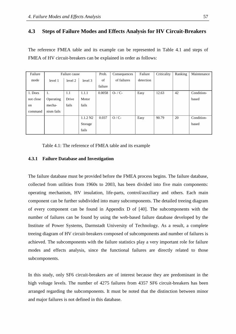
4. Failure Modes and Effects Analysis 57
4.3 Steps of Failure Modes and Effects Analysis for HV Circuit-Breakers
The reference FMEA table and its example can be represented in Table 4.1 and steps of
FMEA of HV circuit-breakers can be explained in order as follows:
Failure cause Failure
mode level 1 level 2 level 3
Prob.
of
failure
Consequences
of failures
Failure
detection
Criticality Ranking Maintenance
1. Does
not close
on
command
1.
Operating
mecha-
nism fails
1.1
Drive
fails
1.1.1
Motor
fails
0.0058 O- / C- Easy 12.63 42 Condition-
based
1.1.2 N2
Storage
fails
0.037 O / C- Easy 90.79 20 Condition-
based
Table 4.1: The reference of FMEA table and its example
4.3.1 Failure Database and Investigation
The failure database must be provided before the FMEA process begins. The failure database,
collected from utilities from 1960s to 2003, has been divided into five main components:
operating mechanism, HV insulation, life-parts, control/auxiliary and others. Each main
component can be further subdivided into many subcomponents. The detailed treeing diagram
of every component can be found in Appendix D of [40]. The subcomponents with the
number of failures can be found by using the web-based failure database developed by the
Institute of Power Systems, Darmstadt University of Technology. As a result, a complete
treeing diagram of HV circuit-breakers composed of subcomponents and number of failures is
achieved. The subcomponents with the failure statistics play a very important role for failure
modes and effects analysis, since the functional failures are directly related to those
subcomponents.
In this study, only SF6 circuit-breakers are of interest because they are predominant in the
high voltage levels. The number of 4275 failures from 4357 SF6 circuit-breakers has been
arranged regarding the subcomponents. It must be noted that the distinction between minor
and major failures is not defined in this database.
4. Failure Modes and Effects Analysis 58
4.3.2 Functions of HV Circuit-Breakers
This is the first step to start the FMEA of HV circuit-breakers. The functions of HV circuit-
breakers can be defined as follows:
• Switching-off operating current
• Switching-on operating current
• Short-circuit current interruption
• Secure open and closed position
The next step is to consider the failures where HV circuit-breakers cannot fulfil the functional
requirements.
4.3.3 Functional Failure Modes of HV Circuit-Breakers
When HV circuit-breakers cannot fulfil the functional requirements as stated in section 4.3.2,
the types of functional failure modes must be defined. Normally, the failures can be divided
into two types of failures: major and minor failures. The minor failures can be prevented by
using scheduled maintenance. In order to do such maintenance, two questions must be
answered:
• What are the causes of failures? • Which events generate the failures?
The possible functional failure modes of HV circuit-breakers according to CIGRE surveys
can be listed as followed:
• Does not close on command • Breakdown to earth
• Does not open on command • Breakdown between poles
• Closes without command • Breakdown across open pole (Internal)
• Opens without command • Breakdown across open pole (External)
• Does not make the current • Locking in open or closed position
• Does not break the current • Others
• Fails to carry the current
4. Failure Modes and Effects Analysis 59
These functional failure modes are listed in the “failure mode” column of FMEA Table as
represented in Table 4.1.
4.3.4 Causes of Failures
This is the process after the functional failures are set up (section 4.3.3). The causes of
functional failures regarding components are considered and categorized. Furthermore, the
detail of the component failures must be investigated with the knowledge from experts and
guidance of IEEE [41]. For example, the failure of an operating mechanism results in the
functional failure modes “Does not close on command”, “Does not open on command”,
“Close without command”, “Open without command” and “Does not break the current”. The
possible causes of failures of an operating mechanism must be figured out. They are then
compared with the failure database; thereby the number of failures can be arranged regarding
components. It must be noted that the failure database is based on the failures of components
without the records of failure modes. Therefore, the proportion of failures from CIGRE, Table
4.2, which occurred in any failure modes, must be applied.
For example, the causes of hydraulic operating mechanism failure in the functional failure
mode “Does not close on command” are composed of: 20 failures of motors, 160 failures of
N2 Storage, 230 failures of connection, 33 failures of values and others. The failure causes in
FMEA Table are subdivided in 3 levels as represented in Table 4.1.
4.3.5 Consequences of Failures
After the causes of failures are classified, the next step of the FMEA is to evaluate the
consequences of failures. The evaluation of the consequences of failures is significant to
figure out the importance of failures. In this study, the consequences of failures are
categorized into four groups:
• Personnel safety
• Environmental impact
• Operation availability/Duration of repair
• Costs of repair
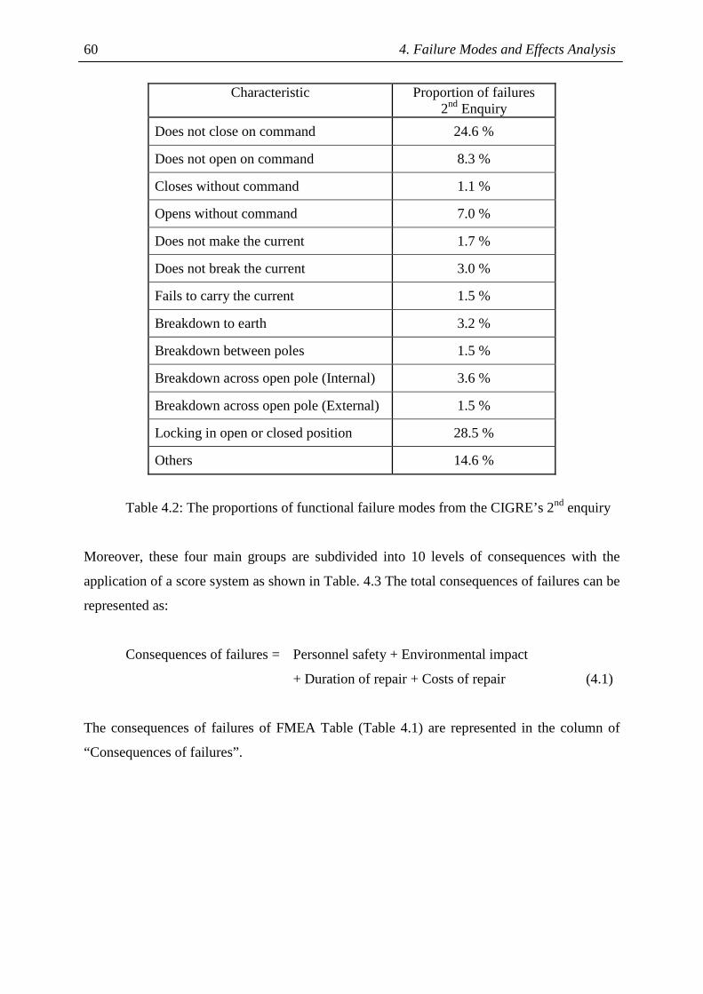
4. Failure Modes and Effects Analysis 60
Characteristic Proportion of failures 2nd Enquiry
Does not close on command 24.6 %
Does not open on command 8.3 %
Closes without command 1.1 %
Opens without command 7.0 %
Does not make the current 1.7 %
Does not break the current 3.0 %
Fails to carry the current 1.5 %
Breakdown to earth 3.2 %
Breakdown between poles 1.5 %
Breakdown across open pole (Internal) 3.6 %
Breakdown across open pole (External) 1.5 %
Locking in open or closed position 28.5 %
Others 14.6 %
Table 4.2: The proportions of functional failure modes from the CIGRE’s 2nd enquiry
Moreover, these four main groups are subdivided into 10 levels of consequences with the
application of a score system as shown in Table. 4.3 The total consequences of failures can be
represented as:
Consequences of failures = Personnel safety + Environmental impact
+ Duration of repair + Costs of repair (4.1)
The consequences of failures of FMEA Table (Table 4.1) are represented in the column of
“Consequences of failures”.
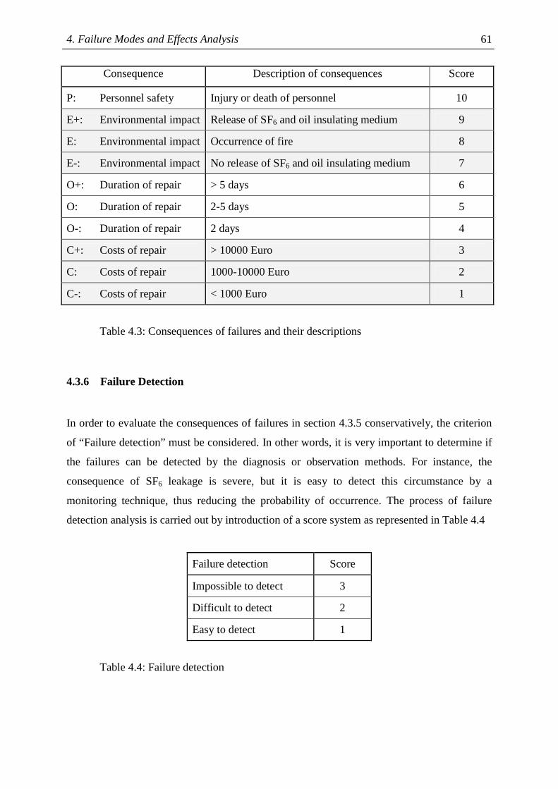
4. Failure Modes and Effects Analysis 61
Consequence Description of consequences Score
P: Personnel safety Injury or death of personnel 10
E+: Environmental impact Release of SF6 and oil insulating medium 9
E: Environmental impact Occurrence of fire 8
E-: Environmental impact No release of SF6 and oil insulating medium 7
O+: Duration of repair > 5 days 6
O: Duration of repair 2-5 days 5
O-: Duration of repair 2 days 4
C+: Costs of repair > 10000 Euro 3
C: Costs of repair 1000-10000 Euro 2
C-: Costs of repair < 1000 Euro 1
Table 4.3: Consequences of failures and their descriptions
4.3.6 Failure Detection
In order to evaluate the consequences of failures in section 4.3.5 conservatively, the criterion
of “Failure detection” must be considered. In other words, it is very important to determine if
the failures can be detected by the diagnosis or observation methods. For instance, the
consequence of SF6 leakage is severe, but it is easy to detect this circumstance by a
monitoring technique, thus reducing the probability of occurrence. The process of failure
detection analysis is carried out by introduction of a score system as represented in Table 4.4
Failure detection Score
Impossible to detect 3
Difficult to detect 2
Easy to detect 1
Table 4.4: Failure detection

4. Failure Modes and Effects Analysis 62
The descriptions of different levels of failure detection can be explained as followed:
• Impossible to detect: The failure cannot be discovered by the maintenance method.
• Difficult to detect: The failure is not be able to be diagnosed or the additional diagnose
must be required.
• Easy to detect: The failure can be detected by the maintenance method.
4.4 Failure Modes and Effects Analysis Evaluation Process
The process of the FMEA, after assembling the required information in section 4.3, can be
represented in Fig. 4.2
Record the functional failure modes
Record the causes of failures for every functional failure mode
Evaluation of failures regarding consequences
Evaluation of failure regarding failure detection
Risk assessment of failures
Probability of failure from the failure database
Ranking risks and evaluation of maintenance programs
Figure 4.2: The flowchart of FMEA evaluation process
It can be seen from Fig. 4.2 that the risk assessment of failures are comprised of the product
of three parameters: consequences, failure detection and probability of failure. The product of
first two parameters, consequences and failure detection, are mentioned as the entire
consequences. The consequence damage with the highest score represents the highest risk of
the considered component. Therefore, the appropriate maintenance program must be applied
to reduce this high risk. Due to the application of the score system for different parameters,
the results of the evaluation are largely dependent on the range of the score scales. In order to

4. Failure Modes and Effects Analysis 63
reduce this effect, the decision matrix approach as shown in Fig. 4.3 must be implemented
[42]. With this method, every 2 parameters are compared with each other, in this case
providing an indication of the risk.
Criteria
A: C
onse
quen
ce
of fa
ilure
B
: Fai
lure
de
tect
ion
C: P
roba
bilit
y of
fa
ilure
ΣΣΣΣ WF/%
A: Consequence of failure 0 1 1 2 16.7
B: Failure detection 3 0 3 6 50.0
C: Probability of failure 3 1 0 4 33.3
12 100.0
Figure 4.3: The decision matrix
The weighting factors with respect to the decision criteria can be defined as follows:
(example)
• The effect of parameter A is smaller than B: 1
• The effect of parameter A is similar to B: 2
• The effect of parameter A is larger than B: 3
The summation of each parameter on the horizontal axis is compared with the total
summation on the vertical axis, resulting in the proportion of each parameter to the total
effect. The evaluation with this method represents the maximum weighting factors that should
be applied for each parameter. The maximum weighting factors for each parameter can be
concluded as followed:
• Consequence of failure 16.7%
• Failure detection 50.0%
• Probability of failure 33.3%

4. Failure Modes and Effects Analysis 64
The weighting factors of the three parameters show that the effect of failure detection plays a
higher significant role for risk assessment than the other two parameters. The equation of risk
assessment composed of three mentioned parameters can be expressed as:
Risk = Consequence of failure x Failure detection x Probability of failure (4.2)
It must be noted that the maximum values of the mentioned parameters from section 4.3.1,
4.3.5 and 4.3.6 must be transformed to match with the maximum weighting factors from the
decision matrix. The transformation method and the related equations are represented in
Appendix A.
4.5 Results of Failure Modes and Effects Analysis
With the FMEA evaluation process, the risk of failure of every component can be
investigated. The damage of one component can lead to many functional failures. For
example, the failure of a motor could result in the functional failures “Does not close on
command” and “Does not open on command”. The priority of risk in relation to functional
failures and damage of components from the FMEA process in section 4.3 is shown in Table
4.5. It is obvious from Table 4.5 which functional failures, from which components, must be
carefully taken into account. The full analysis of FMEA is found in Appendix B1.
In addition, it is very useful to assess the risk with respect to only components, since the
typical maintenance program is designed to maintain the components. The evaluation of risk
based only on components can be represented in Table 4.6. The details of the evaluation can
be found in Appendix B2.

4. Failure Modes and Effects Analysis 65
Priority Score Functional failure Damaged component
1 4011 Does not break the current Controlled capacitor
2 3482 Does not close on command Linkage
3 1530 Does not open on command Linkage
4 1455 Breakdown to earth Porcelain
5 1216 Does not make the current Switching contacts
6 1196 Breakdown to earth Arcing chamber housing
7 1140 Does not close on command SF6 heating equipment
8 1124 Fails to carry current Switching contacts
9 928 Breakdown along open pole (external) Porcelain
10 830 Does not break the current Linkage
11 806 Breakdown across open pole (external) Arcing chamber housing
12 451 Does not open on command SF6 heating equipment
13 187 Does not close on command SF6 leakage/Sealing
14 182 Does not close on command Damping equipment
15 155 Opens without command Trip latch
Table 4.5: The priority of risk in relation to functional failures and damage of
components
Priority Score Damaged component Maintenance strategy
1 3659 Linkage Corrective
2 2999 Controlled capacitor Time-based
3 1421 Porcelain Time-based
4 1414 Switching contacts Time-based
5 1134 Arcing chamber housing Time-based
6 1120 SF6 heating equipment Condition-based
7 222 SF6 leakage/Sealing Condition-based
8 165 Damping equipment Time-based
9 132 Trip latch Corrective
10 111 Sensors Corrective
Table 4.6: The priority of risk with respect to damaged components
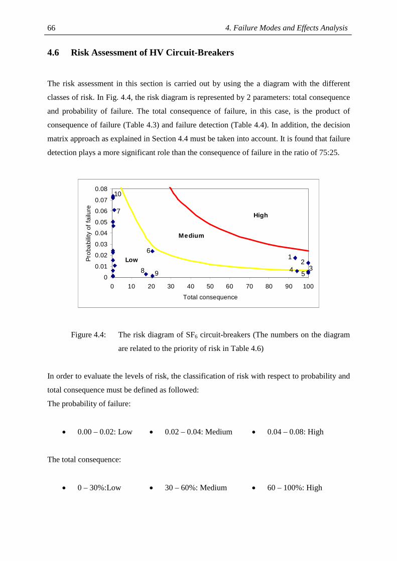
4. Failure Modes and Effects Analysis 66
4.6 Risk Assessment of HV Circuit-Breakers
The risk assessment in this section is carried out by using the a diagram with the different
classes of risk. In Fig. 4.4, the risk diagram is represented by 2 parameters: total consequence
and probability of failure. The total consequence of failure, in this case, is the product of
consequence of failure (Table 4.3) and failure detection (Table 4.4). In addition, the decision
matrix approach as explained in Section 4.4 must be taken into account. It is found that failure
detection plays a more significant role than the consequence of failure in the ratio of 75:25.
0
0.01
0.02
0.03
0.04
0.05
0.06
0.07
0.08
0 10 20 30 40 50 60 70 80 90 100
Total consequence
Pro
babi
lity
of f
ailu
re
Low
Medium
High
4
6
238 9
10
1
5
7
Figure 4.4: The risk diagram of SF6 circuit-breakers (The numbers on the diagram
are related to the priority of risk in Table 4.6)
In order to evaluate the levels of risk, the classification of risk with respect to probability and
total consequence must be defined as followed:
The probability of failure:
• 0.00 – 0.02: Low • 0.02 – 0.04: Medium • 0.04 – 0.08: High
The total consequence:
• 0 – 30%:Low • 30 – 60%: Medium • 60 – 100%: High

4. Failure Modes and Effects Analysis 67
From these criteria, the iso-risk curves can be calculated and plotted as shown in Fig. 4.4.
These iso-risk curves illustrate the identical degrees of risk along the iso-risk curve lines. It
can be concluded from Fig. 4.4 that:
• The components 1 and 2 corresponding “linkage” and “controlled capacitor” are in the
region of “Medium” level of risk. In order to reduce the degree of risk, an improved
maintenance program is recommended. For example, the typical corrective maintenance
of linkage and time-based maintenance of controlled capacitor could be changed to
online condition-based maintenance.
• The components 3, 4 and 5 regarding “porcelain”, “switching contacts” and “arcing
chamber” housing are on the low-medium iso-risk curve. In this case, it is possible to
reduce the risk by introducing the more effective maintenance program. However, it is
not necessary to change the maintenance technique, since the probabilities of failures are
relatively low.
• The component 6, “SF6 heating equipment”, is close to the low-medium boundary. In
order to reduce the risk to the secure position (low region), the condition-based
maintenance should be more frequently carried out. The more frequent condition-based
maintenance can be also applied to component 7, “SF6 sealing”, to reduce the probability
of failure. However, those components are already in the low risk region. It might not be
cost-effective to improve the maintenance program.
• The probabilities of failures from components 8 and 9, “damping equipment” and “trip
latch”, are considerably low. Therefore, it is not necessary to change the maintenance
programs.
• The component 10, “sensors”, has the highest probability of failures but very small
consequence of failure. It is possible to improve or change the maintenance method from
corrective to time-based or condition-based method. However, it is unreasonable to use
the additional monitoring methods for the monitoring devices such as sensors.
It can be concluded in this chapter that the Failure Modes and Effects Analysis (FMEA)
method is very useful method to evaluate the risk of components of HV circuit-breakers.
Consequently, the improved maintenance programs for determined components can be
introduced.


5. Probability and Reliability Models 69
5 Probability and Reliability Models
5.1 Probability Distributions in Reliability Evaluation
Probability distributions are considered as the main parameters in order to evaluate the
reliability of components and systems. These probability distributions correspond to the
time-to-failure of components which are variable due to different types, structures,
manufactures and operating conditions. Practically, the time-to-failure cannot be obtained
directly from the components or systems but must be determined from the sample testing or
from the data collection.
The main types of distributions are divided into two groups: discrete and continuous
distributions. Discrete distributions represent random variables as discrete values which are
normally nonnegative integer values, whereas continuous distributions represent random
variables as real numbers. The two most important discrete distributions are binomial and
Poisson distributions. The frequently-used continuous distributions comprise normal,
exponential, Weibull, gamma and Rayleigh distributions.
The four main probability functions: the reliability function, the cumulative distribution
function, the probability density function and the hazard rate function are introduced in this
chapter. In addition, mean time to failure and mean time to repair are taken into account. The
fundamentals of reliability engineering can be reviewed in [43] and [44]. The focus of
reliability engineering on power systems can be found in [45].
5.1.1 The Reliability Function
The cumulative distribution function, designated by Q(t), is the distribution function
increasing from zero to unity. At time t = 0, the component is just in operation, then Q(t = 0)
is equal to zero. In other words, there is no failure at the beginning of the operation. When the
time reaches infinity (t → ∞), the probability of failure is likely to be unity, since the
component will fail when the time is long enough. In the area of reliability, it is often to
5. Probability and Reliability Models 70
mention the cumulative distribution function in terms of the reliability function, R(t), which is
the complementary value of the cumulative distribution function as represented in Eq. 5.1.
R(t) = 1 - Q(t) (5.1)
In case of a continuous random variable, the probability density function (PDF) can be
obtained by the derivative of the cumulative distribution function. The probability density
function can be mentioned as a failure density function, f(t) .
dQ(t) dR(t)
f(t) = =dt dt
− (5.2)
or t
0
Q(t) = f(t) dt∫ (5.3)
and t
0 t
R(t) = 1 - f(t) dt = f(t) dt∞
∫ ∫ (5.4)
For the discrete random variable, the integrals in Eq. 5.3 and 5.4 are replaced by summations.
The shapes of cumulative distribution function, reliability function and probability density
function are depicted in Fig. 5.1
5.1.2 Failure Rate Function
The failure rate or hazard rate function, λ(t), is one of the most important functions in
reliability analysis. It is described as a transition rate of failure over a period of time. This
function is dependent on the number of failures in a specified period of time and the number
of components subject to failure.
number of failure per unit time
λ(t) =number of components exposed to failure
(5.5)
The general reliability functions can be represented and explained by simple equations as
follows:
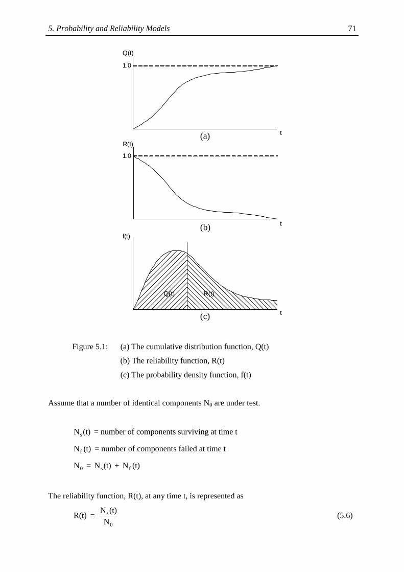
5. Probability and Reliability Models 71
Q(t)
t
R(t)
t
f(t)
t
1.0
1.0
(a)
(b)
(c)
Q(t) R(t)
Figure 5.1: (a) The cumulative distribution function, Q(t)
(b) The reliability function, R(t)
(c) The probability density function, f(t)
Assume that a number of identical components N0 are under test.
sN (t) = number of components surviving at time t
fN (t) = number of components failed at time t
0 s fN = N (t) + N (t)
The reliability function, R(t), at any time t, is represented as
s
0
N (t)R(t) =
N (5.6)
5. Probability and Reliability Models 72
= 0 f
0
N - N (t)
N = f
0
N (t)1 -
N (5.7)
Likewise, the cumulative distribution function Q(t) is
f
0
N (t)Q(t) =
N (5.8)
From Eq. 5.2, the probability density function can be calculated as
dQ(t) -dR(t)
f(t) = =dt dt
f
0
1 dN (t)f(t) =
N dt⋅ , when dt → 0 (5.9)
Comparing the equations 5.5 and 5.9, the failure rate and the probability density function are
identical at time t = 0. The general equation of failure rate at time t can be expressed as
f
s
1 dN (t)λ(t) =
N (t) dt⋅ 0 f
0 s
N 1 dN (t)=
N N (t) dt⋅ ⋅
0 f
s 0
N 1 dN (t)=
N (t) N dt⋅ ⋅
1= f(t)
R(t)⋅ (5.10)
or -1 dR(t)
=R(t) dt
⋅ (5.11)
The reliability function R(t) can be derived from failure rate function as follows:
-1 dR(t)
λ(t) =R(t) dt
⋅ -dR(t)
λ(t)dt =R(t)
Integrating,
R(t)t
0 1
1-λ(t)dt = dR(t)
R(t)⋅∫ ∫
t
0
-λ(t)dt = lnR(t)∫
5. Probability and Reliability Models 73
t
0
R(t) = exp - λ(t)dt ∫ (5.12)
5.1.3 Mean Time to Failure
The mean time to failure (MTTF) or expected value can be defined as
0
MTTF = E(T) = t f(t)dt∞
⋅∫ : continuous distribution (5.13)
or xx=0
MTTF = E(X) = x P∞
⋅∑ : discrete distribution (5.14)
Substituting the Eq. 5.2 into Eq. 5.13 results in
0
dR(t)MTTF = - tdt
dt
∞
⋅∫
0
0
MTTF = -t R(t) + R(t)dt∞
∞⋅ ∫
0
MTTF = R(t)dt∞
∫ (5.15)
The mean time to failure is one of several measures to represent the central tendency of the
failure distribution. The other important parameters are the median time to failure, tmed, and
the mode, tmode. The median time to failure divides the failure distribution into two halves
(50:50), while the mode represents the maximum value of the failure distribution.
medR(t ) = 0.5 (5.16)
mode0 t<
f(t ) = max f(t)≤ ∞
(5.17)
The example of MTTF, the median and the mode are shown in Fig. 5.2

5. Probability and Reliability Models 74
t
f(t)
tmode tmed MTTF
Figure 5.2: The example of MTTF, the median and the mode
It is obvious from Fig. 5.2 that only the MTTF cannot represent the shape of failure
distribution. The other measure which can be used to describe the shape of failure distribution
is variance, σ2, expressed by
2 2
0
σ = (t - MTTF) f(t)dt∞
⋅∫
2 2 2
0
σ = t f(t) dt - (MTTF)∞
⋅ ⋅∫ (5.18)
5.1.4 The Exponential Distribution
The exponential distribution is one of the most important distributions in a reliability
evaluation. It has a constant failure rate (λ) which is the characteristic of the components in
the useful life region of bathtub curve. The meaning behind the constant failure rate is that the
failures occur randomly. In other words, the time-to-failure of a component is independent to
the period of time that a component has been operated. For example, the probability of failure
of a component in the next 10 years is the same as the probability in the first few years. This
characteristic of the exponential distribution is mentioned as memoryless property.
According to Eq. 5.12, the reliability function R(t) with the constant failure rate, λ(t) = λ ,
can be represented as

5. Probability and Reliability Models 75
t
-λt
0
R(t) = exp - λdt = e ∫ (5.19)
and -λtQ(t) = 1-e
Therefore, the probability density function, mean time to failure and variance are represented
as
-λtdR(t)f(t) = - = λe
dt (5.20)
-λt
0 0
MTTF = R(t)dt = e dt∞ ∞
∫ ∫ -λt
0
e 1MTTF = =
-λ λ
∞
(5.21)
2
2 -λt2
0
1 1σ = 1 - λe dt =
λ λ
∞ ∫ (5.22)
In order to prove the memoryless property of the exponential distribution, the conditional
probability and Fig. 5.3 are applied.
f(t)
tT0 T0+t
Figure 5.3: The memoryless property of exponential distribution
00 0
o
R(T + t)R(T + t|T ) =
R(T )
[ ][ ]
0
0
exp -λ(T + t)=
exp -λT
0
0
exp(-λT ) exp(-λt)=
exp(-λT )
⋅ -λt= exp(-λt) = e = R(t) (5.23)
[ ]0 0R(T +t) = exp -λ(T +t)
[ ]0 0R(T +t/T ) = exp -λt

5. Probability and Reliability Models 76
5.1.5 The Weibull Distribution
The Weibull distribution is the most important distribution to analyse and predict failures of
components. According to the bathtub curve, Fig. 5.4, it can identify the distributions of
infant mortality (region 1), constant failure (region 2) and wear-out (region 3). The Weibull
distribution was found by Waloddi Weibull (1887-1979) who defined the model of a product
life as a function of
β-1 β
β t tf(t) = exp -
α α α
(5.24)
hf
t
Region 1 Region 2 Region 3
Figure 5.4: Bathtub curve
The relevant equations of Weibull distribution are
t
R(t) = f(t)dt∞
∫
β
tR(t) = exp -
α
(5.25)
β-1
β tλ(t) =
α α
(5.26)
The β is referred to the shape parameter of the distribution. The different values of β represent
the different shapes of distribution as follows:
• β < 1: the Weibull distribution has a hyperbolic shape and f(0) = ∞. The distribution
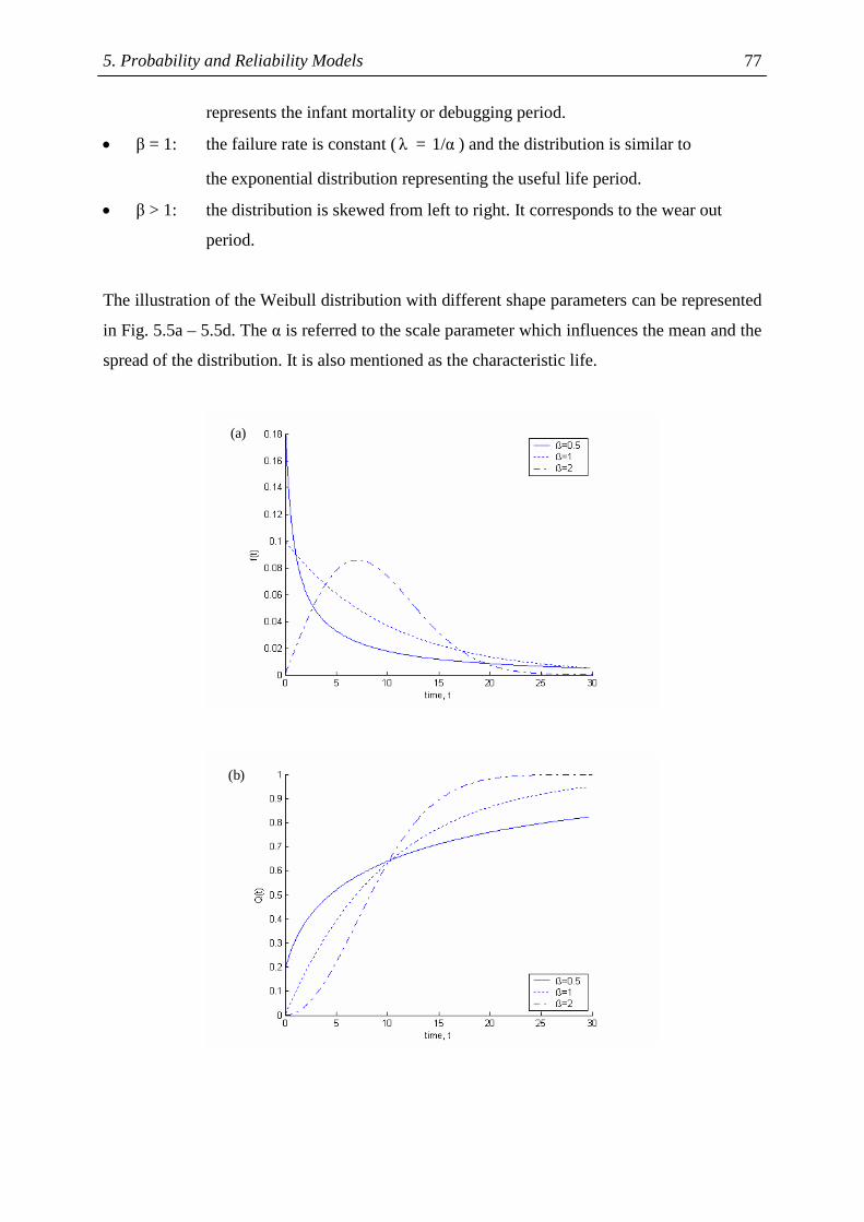
5. Probability and Reliability Models 77
represents the infant mortality or debugging period.
• β = 1: the failure rate is constant (λ = 1/α ) and the distribution is similar to
the exponential distribution representing the useful life period.
• β > 1: the distribution is skewed from left to right. It corresponds to the wear out
period.
The illustration of the Weibull distribution with different shape parameters can be represented
in Fig. 5.5a – 5.5d. The α is referred to the scale parameter which influences the mean and the
spread of the distribution. It is also mentioned as the characteristic life.
(a)
(b)

5. Probability and Reliability Models 78
(c)
(d)
Figure 5.5: The Weibull distribution with different shape parameters, β
(a): The probability density function, f(t)
(b): The cumulative distribution function, Q(t)
(c): The reliability function, R(t)
(d): The failure rate, λ
5.2 Treeing Model
The treeing Model of HV circuit-breakers is the reliability model which is composed of the
distribution of consecutive failures. The aim of this model is to investigate when the failures

5. Probability and Reliability Models 79
occur and what probabilities are during the lifetime. The conditional probability method is
applied to investigate the probabilities of failures from a new status to the first and second
failure in subsequent years. As a result, the critical years of which the failures frequently
occur can be figured out.
5.2.1 Concepts and Diagram
The failures of HV circuit-breakers up to their second failures are taken into account. The
failures of each circuit-breaker can be represented with respect to time, for example, as shown
in Fig. 5.6.
t (year)
new status 1st failure 2nd failure next failures
0 5 10 15
Figure 5.6: The occurrence of failures with respect to time
It can be concluded from Fig. 5.6 that the first failure occurs at the fourth year and the second
failure on the tenth year. Such information is taken for every HV circuit-breaker. The steps of
establishing the treeing diagram can be explained as follows:
1. The failure-free durations of HV circuit-breakers are extracted from the database. For
instance, the failure-free durations of the circuit-breaker in Fig. 5.6 are 4 years from the
new status to the first failure and 6 years from the first to the second failure.
2. The numbers of failures with respect to the failure-free durations are arranged. Therefore,
the numbers of failures in any years are made available.
3. The counting program developed in MATLAB is applied to count the number of circuit-
breakers under specified time conditions. For example, there are 11 HV circuit-breakers
having the first failure in the first year and the second failure in the third year.
4. With the conditional probability method, the treeing diagram of failures is established.
5. The two-dimensional diagram of HV circuit-breakers in relation to the number of failures
is applied.

5. Probability and Reliability Models 80
The formula of conditional probability is
P(A B)
P(A|B) =P(B)
∩ (5.27)
where P(A|B) is the probability of A given B. The treeing diagram of all types of HV circuit-
breakers is represented in Fig 5.7. In this figure, the number of circuit-breakers subject to
failures and their conditional probabilities in any years are written. For example, there are 190
from the total of 9305 circuit-breakers exposed to the first failure in the first year. From those
190 circuit-breakers, there are 36 subject to the second failure within the next 6 months. This
treeing diagram can be illustrated as a two-dimensional diagram in Fig. 5.8. It shows how
many circuit-breakers exposed to the second failures and at which years. For example, it can
be read from Fig. 5.8 that the highest number of circuit-breakers subject to the second failures
is 36. Those 36 circuit-breakers had the first failures in the first year and the second failures in
the next 6 months. More detail as to the number of circuit-breakers subject to the second
failures can be read from Table 5.1.
Using Fig. 5.7 and Table 5.1, the critical paths of the development of failures can be figured
out. When only the first failures are considered, it is obvious that the failures most frequently
occur in the sixth year (252 out of 9305 CBs). The second highest failure amount takes place
in the first year (190 out of 9305 CBs). After that, the second failures are taken into
consideration. It is seen that the most critical path represents the first failure in the first year
and the second failure in the same year (36 out of 9305 CBs). The second most critical path
shows the first failure in the sixth year and the second failure in the same year (28 out of 9305
CBs). In order to make this information easy to be compared with information from other
types of circuit-breakers, the years of the second failures must be transformed with respect to
the starting point. The first five critical paths are listed in Table 5.2.

5. Probability and Reliability Models 81
New status
< 6 months
1st year
2nd year
3 rd year
4 th year
5 th year
6 th year
7 th year
< 6 months
1st year
2nd year
The first failure The second failure
80/9305
190 /9305
165 /9305
112 /9305
181 /9305
252 /9305
126 /9305
98/9305
36/190
21/190
11/190
< 6 months
1st year
2nd year
28/252
11/252
16/252
No failure
8 th year132 /9305
< 6 months
1st year
2nd year
24/181
11/181
6/181
< 6 months
1st year
2nd year
23/165
20/165
13/165
< 6 months
1st year
2nd year
23/126
9/126
11/126
< 6 months
1st year
2nd year
14/80
10/80
5/80
< 6 months
1st year
2nd year
18/112
8/112
5/112 < 6
months
1st year
2nd year
16/98
9/98
9/98
< 6 months
1st year
2nd year
19/132
10/132
6/132
Figure 5.7: Treeing diagram of all types of HV circuit-breakers
Figure 5.8: Two-dimensional diagram representing the number of failures with
respect to time
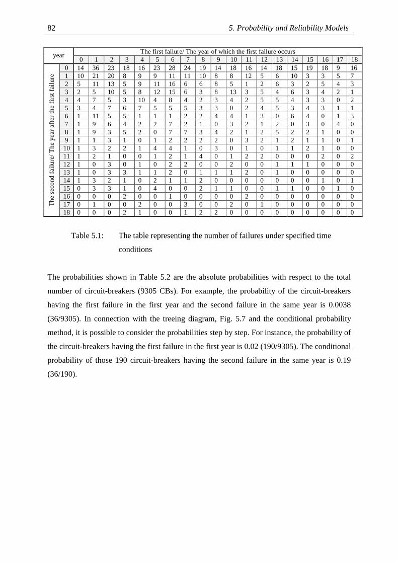
5. Probability and Reliability Models 82
The first failure/ The year of which the first failure occurs year 0 1 2 3 4 5 6 7 8 9 10 11 12 13 14 15 16 17 18
0 14 36 23 18 16 23 28 24 19 14 18 16 14 18 15 19 18 9 16 1 10 21 20 8 9 9 11 11 10 8 8 12 5 6 10 3 3 5 7 2 5 11 13 5 9 11 16 6 6 8 5 1 2 6 3 2 5 4 3 3 2 5 10 5 8 12 15 6 3 8 13 3 5 4 6 3 4 2 1 4 4 7 5 3 10 4 8 4 2 3 4 2 5 5 4 3 3 0 2 5 3 4 7 6 7 5 5 5 3 3 0 2 4 5 3 4 3 1 1 6 1 11 5 5 1 1 1 2 2 4 4 1 3 0 6 4 0 1 3 7 1 9 6 4 2 2 7 2 1 0 3 2 1 2 0 3 0 4 0 8 1 9 3 5 2 0 7 7 3 4 2 1 2 5 2 2 1 0 0 9 1 1 3 1 0 1 2 2 2 2 0 3 2 1 2 1 1 0 1 10 1 3 2 2 1 4 4 1 0 3 0 1 0 1 1 2 1 0 0 11 1 2 1 0 0 1 2 1 4 0 1 2 2 0 0 0 2 0 2 12 1 0 3 0 1 0 2 2 0 0 2 0 0 1 1 1 0 0 0 13 1 0 3 3 1 1 2 0 1 1 1 2 0 1 0 0 0 0 0 14 1 3 2 1 0 2 1 1 2 0 0 0 0 0 0 0 1 0 1 15 0 3 3 1 0 4 0 0 2 1 1 0 0 1 1 0 0 1 0 16 0 0 0 2 0 0 1 0 0 0 0 2 0 0 0 0 0 0 0 17 0 1 0 0 2 0 0 3 0 0 2 0 1 0 0 0 0 0 0 T
he
seco
nd
failu
re/ T
he
year
aft
er th
e fir
st f
ailu
re
18 0 0 0 2 1 0 0 1 2 2 0 0 0 0 0 0 0 0 0
Table 5.1: The table representing the number of failures under specified time
conditions
The probabilities shown in Table 5.2 are the absolute probabilities with respect to the total
number of circuit-breakers (9305 CBs). For example, the probability of the circuit-breakers
having the first failure in the first year and the second failure in the same year is 0.0038
(36/9305). In connection with the treeing diagram, Fig. 5.7 and the conditional probability
method, it is possible to consider the probabilities step by step. For instance, the probability of
the circuit-breakers having the first failure in the first year is 0.02 (190/9305). The conditional
probability of those 190 circuit-breakers having the second failure in the same year is 0.19
(36/190).

5. Probability and Reliability Models 83
Critical path The first failure/ year of which the fist
failure occurs
The second failure/ year of which the second
failure occurs
Probability under specified
conditions
1 1st year 1st year 0.0038 (36/9305)
2 6th year 6th year 0.0030 (28/9305)
3 7th year 7th year 0.0026 (24/9305)
4 2nd year 2nd year 0.0025 (23/9305)
5 5th year 5th year 0.0025 (23/9305)
Table 5.2: The critical paths of the failures
5.2.2 Results of Treeing Diagram
In addition to the investigation of all types of HV circuit-breakers, the treeing models of four
specified types of HV circuit-breakers, SF6 with hydraulic drive, SF6 with mechanical drive,
minimum oil with hydraulic drive and with mechanical drive, are established and
investigated. The first five critical paths of different types of HV circuit-breakers are listed in
Table 5.3. The two-dimensional diagrams of these types of circuit-breakers are represented in
Appendix C.
SF6 with hydraulic drive (3168 CBs)
SF6 with mechanical drive (1220 CBs)
Min. oil with hydraulic drive (1076 CBs)
Min. oil with mechanical drive
(1674 CBs)
Cri
tical
pat
h
1st failure (year)
2nd failure (year)
Prob. 1st failure (year)
2nd failure (year)
Prob. 1st failure (year)
2nd failure (year)
Prob. 1st failure (year)
2nd failure (year)
Prob.
1 1st 1st 0.010 16th 16th 0.007 26th 26th 0.006 23rd 23rd 0.003
2 6th 6th 0.009 10th 10th 0.002 6th 14th 0.006 27th 27th 0.003
3 7th 7th 0.007 1st 1st 0.002 14th 20th 0.005 29th 29th 0.003
4 2nd 2nd 0.006 2nd 4th 0.002 19th 19th 0.005 5th 8th 0.002
5 2nd 3rd 0.006 10th 13th 0.002 22nd 22nd 0.005 17th 24th 0.002
Table 5.3: The comparison of critical paths of different types of circuit-breakers
It must be noted that the probabilities in Table. 5.3 are the absolute probabilities related to the
total population of each respective type. It can be concluded from the treeing models that:

5. Probability and Reliability Models 84
• The second failures which occur in the same year as the first failures are probably
considered as the failures from human error or imperfect repair.
• It is obvious that the probabilities of failures of SF6 circuit-breakers with hydraulic drives
are higher than other types of circuit-breakers.
• It is likely that, the first failures occurring in the first 2-3 years are failures in infant
mortality or in the debugging period.
• When failures in the debugging period are neglected, the failures of SF6 circuit-breakers
with hydraulic drives most frequently occur at the sixth year, whereas those for SF6
circuit-breakers with mechanical drives take place at the sixteenth year. It is obvious that
the reliability of circuit-breakers with mechanical drives is higher than ones with
hydraulic drives.
• Most of the failures of minimum oil circuit-breakers frequently occur after the 20th year.
It is because of the aging phenomena. However, there are some failures found in the first
ten years.
• The probabilities of failures of SF6 circuit-breakers over 20 years are lower than the first
20 years due to the fact that a great number of SF6 circuit-breakers have not reached the
aging period. It might be very interesting to further collect the failure database in the next
20 years and use this treeing diagram to investigate the critical paths again.
The advantages of treeing diagram can be concluded as followed:
• With the conditional probability method, it is possible to determine the probability of
failures at any specified time condition.
• The treeing model can be used to establish the adaptive maintenance programs or at least
to provide valuable information for asset managers and maintenance personnel as to
when “the following failures” are likely to occur. The adaptive maintenance program can
be explained by using the example of SF6 circuit-breakers with hydraulic drives. It is
clear that the first failures frequently occur in the 6th-7th year. The maintenance program
should be introduced before this time to reduce the probability of failures. Afterwards, it
can be found in the treeing diagram that the second failures frequently occur within 1-3
year after the first failures. This is the information for the asset managers and
maintenance personnel to be aware of the following failures coming in the near future.
• The treeing diagram can be expanded to study the third and fourth failures but it requires
required a more complicated filter and counting program.

5. Probability and Reliability Models 85
5.3 Cascading Reliability Model
A cascading reliability model can be considered as the extension of treeing model. The main
difference is the reliability point of view. The cascading reliability model determines the
reliability of consecutive failures in terms of the mean time to failure (MTTF), state and
transition probabilities. In this model, the failure database of different types of HV circuit-
breakers from the 1960s is applied in order to investigate reliability. With the cascading
reliability model, the durations between failures or mean time to failure (MTTF) between
consecutive failures are investigated. Consequently, the failure development trend from the
first to the second and the third failure can be determined. The exponential reliability
distributions of the first, second, and third failures are introduced in terms of the cascading
reliability model. As a result, the probabilities and availabilities of HV circuit-breakers
subject to consecutive failures can be investigated. For example, with this cascading
reliability model, the probability that circuit-breakers are subject to the first failure within 10
years, the second failure within the next 5 years and the third failure within the next 3 years
can be discovered.
Other probabilistic models applied to HV circuit-breakers can be found in [46] and [47]. The
aging probability with an effect of maintenance on reliability and costs is discussed in [48].
5.3.1 Investigation of Failure Database
In this section, the preparation of failure data and investigation of reliability parameters are
described. It must be noted that five different groups (all types, SF6 with hydraulic drive, SF6
with mechanical drive, minimum oil with hydraulic drive and with mechanical drive) had
been studied. According to small samples of air blast circuit-breakers, they were not
separately considered.
5.3.1.1 Investigation of failure-free time of HV circuit-breakers
Since the 1960s, every failure regardless of major and minor failures had been recorded in the
database. Accordingly, failures are considered without the distinction between major and
minor failures. The structure of the failure database can be reviewed from [49] and [50]. The

5. Probability and Reliability Models 86
durations between failures of HV circuit-breakers are extracted from the database, thus
forming the failure-free times. As a result, the distribution between numbers of failures and
failure-free times can be established. For example, the HV circuit-breaker has 3 failures in the
10th, 17th, and 24th year. It can be seen that the first failure occurs in the 10th year, the second
failure in the next 7 years and the third failure in the following 7 years. From the whole
population, the failure-free times of the first failures are then collected and the distribution is
formed. The second and the third failure-free times can be carried out in the same way.
Finally, the distributions of the first, second, and third failures are connected in series, thus
forming the cascading reliability model. The average failure-free time can be represented as
follows.
n
i ii=1
E(x)= X P⋅∑ (5.28)
where Xi: the failure-free time i (year)
Pi: the probability of failures at failure-free time i
5.3.1.2 Reliability parameters
This average failure-free time can be represented as the mean time to failure (MTTF). For
example, the MTTF1, MTTF2, and MTTF3 represent the average failure-free times from no
failure to the first failure, the first to the second failure, and the second to the third failure
respectively. These MTTFs and their distributions are then connected in series to form the
cascading reliability model. When the distribution of failures can be represented by an
exponential distribution, the failure rate (λ) is then calculated by inverse of MTTF. In
conclusion, the exponential reliability distributions, MTTFs and failure rates of different types
of HV circuit-breakers are investigated and the failure developments are then compared.
5.3.1.3 Precautions of evaluation of reliability parameters
Precautions in the evaluation of reliability parameters must be taken into account in order to
reduce inaccuracy of reliability parameters; for example:

5. Probability and Reliability Models 87
• Due to lack of commissioning date information, the manufacturing date is then applied as
the starting time. For the first failures, ones occurring in the first 3 years can be considered
as the failures in the burn-in period. MTTFs with and without consideration of this period
are compared.
• For the second failures, ones occurring on the same day or in the next few months after
the first failures are considered as repetitive failures resulting from human error and
incomplete repair/inspection. Consequently, the expected values or MTTFs are reduced.
The third and following failures can be treated by the same assumption.
5.3.2 Principle of Cascading Reliability Model
The cascading reliability model of HV circuit-breakers can be described as the connection of
reliability distributions of the first, second and following failures in series. The probabilities
of each state, between states and the reliability distributions can be investigated. The
cascading reliability model of HV circuit-breakers can be represented in Fig. 5.9.
No failure
P01st failure
P12nd failure
P23rd failure
P3
P01
MTTF1
P12
MTTF2
P23
MTTF3
Figure 5.9: The cascading reliability model of HV circuit-breakers
The probabilities P0, P1, P2 and P3 represent the state probabilities, whereas the probabilities
P01, P12, P23 show the transition probabilities between states. The state probabilities are the
probabilities of residing in any states. For example, the state probability P0 is the probability
of circuit-breakers staying in failure-free state. The transition probabilities are the
probabilities between states. For example, the transition probability P12 is the probability of
failure development from the first to the second failure. MTTFs and their exponential
reliability distributions represent the development of failures between states. In other words,
the durations between failures and their probabilities can be investigated by using this
cascading reliability model. It must be noted that, MTTFs are investigated from the database
in which the general maintenance programs are already included. It means that, the influence
of general maintenance programs to MTTFs is already included.
5. Probability and Reliability Models 88
5.3.2.1 Reliability and availability of cascading reliability model
The reliability and availability of the cascading reliability model can be classified into two
categories: the real case and the approximated case by using an exponential distribution. The
real reliability can be investigated from the real distribution of failures, whereas the
approximate reliability can be derived from the exponential reliability distribution. The
exponential reliability distribution and its related equations are represented in Section 5.1.4.
The survivor function, R(t), for the HV circuit-breakers having many failures can be
examined by connecting the exponential functions of every failure in series leading to the
cascading reliability model. In this study, HV circuit-breakers having up to 3 failures are
considered. The survivor function, R(t), of HV circuit-breakers subject to 3 failures can be
represented as
3 3 21 1 2 2 1 -λ (t -t )-λ t -λ (t -t )R(t) = e e e⋅ ⋅ (5.29)
3 21 2 1 -(t -t )/MTTF3-t /MTTF1 -(t -t )/MTTF2R(t) = e e e⋅ ⋅ (5.30)
λ1, λ2, λ3: failure rate of the first, second, and third failure
t1,t2,t3: The time of the first, second, and third failure
MTTF1, 2, and 3: Mean time to failure of the first, second, and third failure
For example, the survivor function, R(t), of HV circuit-breakers having the first failure within
10 years, the second failure within the next 5 years, and the third failure within the next 3
years can be calculated as 31 2 -λ (3)-λ (10) -λ (5)R(t) = e e e⋅ ⋅ .
5.3.3 Results of Investigation
The results of investigation can be divided into two parts. The first part represents the failure
development from the beginning to the last failures. Due to small numbers of HV circuit-
breakers having more than 3 failures, only the cascading model up to 3 failures is illustrated.
The state probabilities and transition probabilities can be examined from the model. The
second part represents the exponential reliability distributions of the cascading reliability
model.

5. Probability and Reliability Models 89
5.3.3.1 State and transition probabilities of cascading reliability model
The state and transition probabilities of the cascading reliability model with respect to Fig. 5.9
can be summarized in Table 5.4. This table shows the different types of circuit-breakers
subject to failures and how those failures transit from state to state. For example, SF6 circuit-
breakers with mechanical drive stay in the failure-free state, P0, 83 % and the transition
probability from the failure-free to the first failure state, P01, is 17%. The MTTFs with and
without the consideration of burn-in period and repetitive failures (according to the section
5.3.1.3) are represented in Table 5.5. These MTTFs represent how fast the failures occur from
state to state. For instance, SF6 circuit-breakers with mechanical drive stay 10.74 years
(MTTF1) until the first failures occur. After that, the second failures occur 2.09 years
(MTTF2) later.
State probability Transition probability Type of CB P0 P1 P2 P3 P01 P12 P23
All types 0.66 0.18 0.07 0.03 0.34 0.47 0.56
SF6 with hydraulic drive 0.47 0.25 0.12 0.06 0.53 0.53 0.59
SF6 with mechanical drive 0.83 0.13 0.03 0.01 0.17 0.23 0.28
Min. oil with hydraulic drive 0.45 0.27 0.12 0.07 0.55 0.51 0.59
Min. oil with mechanical drive
0.83 0.10 0.03 0.01 0.17 0.42 0.51
Table 5.4 State and transition probabilities of different types of HV
circuit-breakers
with burn-in period and
repetitive failures without burn-in period and
repetitive failures Type of CB
MTTF1 (year)
MTTF2 (year)
MTTF3 (year)
MTTF1 (year)
MTTF2 (year)
MTTF3 (year)
All types 12.35 3.43 2.25 14.62 5.11 4.09
SF6 with hydraulic drive 7.79 3.30 2.35 10.10 4.84 4.00
SF6 with mechanical drive 10.74 2.09 2.85 14.06 3.5 4.63
Min. oil with hydraulic drive 16.96 4.68 2.30 17.68 6.44 4.44
Min. oil with mechanical drive
18.99 3.14 2.45 19.23 5.69 5.25
Table 5.5 Mean time to failures of different types of HV circuit-breakers

5. Probability and Reliability Models 90
It can be seen from Table 5.5 that MTTF3s are shorter than MTTF2s and MTTF1s
respectively. In other words, the following failures occur faster than the previous ones. The
state probabilities and MTTFs can be illustrated in Fig. 5.10 and 5.11 respectively. The
summation of state probabilities of each type of circuit-breaker is equal to unity, but only the
summation to state P3 is represented in Fig. 5.10. It is apparent that more than 90 % of HV
circuit-breakers are not exposed to more than 3 failures. It can be seen that more than 80 % of
HV circuit-breakers with mechanical drives stay in failure-free state, P0. It could be
concluded that HV circuit-breakers with mechanical drives have higher reliability than HV
circuit-breakers with hydraulic drives.
0
0.1
0.2
0.3
0.4
0.50.6
0.7
0.8
0.9
1
All types SF6-hy SF6-mech Oil-hy Oil-mech
Types of circuit-breakers
Sta
te p
roba
bilit
ies
P3
P2
P1
P0
Figure 5.10: State probabilities of different types of HV circuit-breakers
0 5 10 15 20 25 30 35
All types(b)All types(a)
SF6-hy(b)SF6-hy(a)
SF6-mech(b)SF6-mech(a)
Oil-hy(b)Oil-hy(a)
Oil-mech(b)Oil-mech(a)
Typ
es o
f H
V c
ircui
t-br
eake
rs
Mean time to failures, MTTFs, (year)
MTTF1 MTTF2 MTTF3
Figure 5.11: Mean time to failures of different types of circuit-breakers
(a): with consideration of burn-in period and repetitive failures
(b): without consideration of burn-in period and repetitive failures

5. Probability and Reliability Models 91
The failure development in terms of MTTFs can be explained from Fig. 5.11. It is obvious
that without the consideration of burn-in period and repetitive failures, the cascading MTTF
(MTTF1, MTTF2, and MTTF3) is extended up to around 6 years. The effect of human error
and incomplete repair/inspection can be derived from Table 5.5 and Fig. 5.11. For example, in
case of all types of HV circuit-breakers, MTTF2 can be extended up to 49 % without the
consideration of repetitive failures. In other words, a perfect repair/inspection is able to extend
MTTF2 up to 1.68 years or 49% in case of all types of HV circuit-breakers.
5.3.3.2 The exponential reliability distributions of the cascading reliability model
The exponential reliability distributions of the cascading reliability model are composed of
three distributions of failures connected in series. Examples of the exponential reliability
distributions of SF6 circuit-breakers with hydraulic drives are depicted in Fig. 5.12. It is
obvious that the failure development of the third failure is faster than the second and the first
failure respectively. The cumulative distribution function or probability of failure, Q(t), and
the survivor function, R(t), can be calculated by using Eq. (5.1), (5.29) and (5.30).
For instance, the survivor function, R(t), of the SF6 circuit-breakers with hydraulic drives
having the first failure within 10 years, the second failure within the next 5 years, and the
third failure within the next 3 years, can be calculated by using MTTFs from Table 5.5 as
follows:
-10/MTTF1 -(15-10)/MTTF2 -(18-15)/MTTF3R(t) = e e e⋅ ⋅
-10/10.1 -5/4.84 -3/4.0R(t) = e e e = 0.0625⋅ ⋅
Q(t) = 1-R(t) = 1-0.0625 = 0.9375
The interpretation of the calculation must be carefully paid attention. For the above example,
it can be concluded that SF6 circuit-breakers with hydraulic drives having exactly 3 failures
will have the survivor function of 6.25 % when the above time conditions are taken into
account. In other words, the probability of failure of SF6 circuit-breakers in these conditions is
93.75 %. However, the population of the SF6 circuit-breakers with hydraulic drives having
exactly 3 failures, state P3, represents only 6 % of the total population of this type.

5. Probability and Reliability Models 92
0
0.02
0.04
0.06
0.08
0.1
0.12
0 2 4 6 8 10 12 14 16 18 20 22 24 26 28 30 32
failure-free time (year)
f(t)
0
0.05
0.1
0.15
0.2
0.25
0 2 4 6 8 10 12 14 16 18 20 22
failure-free time (year)
f(t)
0
0.05
0.1
0.15
0.2
0.25
0.3
0 1 2 3 4 5 6 7 8 9 10 11 12 13 14 15 16 17 18
failure-free time (year)
f(t)
Fig. 5.12: The exponential reliability distributions of SF6 circuit-breakers with
hydraulic drives (without consideration of burn-in period and repetitive
failures)
(a): The first failure (b): The second failure (c): The third failure
When the survivor function up to the second failure (the first failure within 10 years and the
second failure within the next 5 years) is considered, the calculation is then carried out as
follows:
(a)
(b)
(c)

5. Probability and Reliability Models 93
-10/MTTF1 -(15-10)/MTTF2R(t) = e e⋅
-10/10.1 -5/4.84R(t) = e e = 0.1323⋅
Q(t) = 1-R(t) = 1-0.0625 = 0.8677
It can be concluded in the same way that SF6 circuit-breakers with hydraulic drives having
exactly 2 failures will have the survivor function of 13.23 % when the above time conditions
are given. The probability of failure in this case is 86.77 %. The population of this type of
circuit-breakers having exactly 2 failures, state P2, corresponds to 12 % of the total
population. The survivor function of SF6 circuit-breakers with hydraulic drives having only
one failure within 10 years is 0.37 %. The population of this type of circuit-breaker having
only one failure, state P1, is 25 % of the total population.
In order to compare the survivor functions of different types of HV circuit-breakers, the
identical time conditions must be taken into account. On the other hand, the time conditions
can be compared when a similar survivor function is considered. For example, the time
conditions of HV circuit-breakers having exactly 3 failures (the first failure within 10 years,
the second failure within the next 5 years, and the third failure within the next 3 years) are set,
and the survivor functions of different types of HV circuit-breakers are then compared.
• SF6 with hydraulic drives: R(t) = 0.0625
• SF6 with mechanical drives: R(t) = 0.0616
• Minimum oil with hydraulic drives: R(t) = 0.133
• Minimum oil with mechanical drives: R(t) = 0.139
It is obvious in the comparison that minimum oil circuit-breakers have approximately 2 times
higher survivor function than SF6 circuit-breakers under a similar condition. Furthermore, the
state probability P3 must be taken into consideration to compare the percentage of the
population at this state. It can be seen from Table 5.4 that the population of HV circuit-
breakers with mechanical drives (SF6 and minimum oil circuit-breakers) at state P3 represents
only 1 % of the total population of its type, whereas the circuit-breakers with hydraulic drives
show 6-7 %. It is then concluded that the HV circuit-breakers with mechanical drives have
higher reliability than HV circuit-breakers with hydraulic drives.

5. Probability and Reliability Models 94
5.3.4 Conclusions
The following can be concluded from the investigation of the cascading reliability model of
HV circuit-breakers:
• The cascading reliability model of HV circuit-breakers is composed of state probabilities,
transition probabilities, and reliability distributions. This model is very useful to study the
probability of failures and availability of circuit-breakers in any states. It is also beneficial
for maintenance personnel to be aware of the first and following failures.
• State probabilities represent the probabilities of circuit-breakers residing in any states. For
instance, state P0 shows the probability of HV circuit-breakers having no failure and state
P1 represents the probability of HV circuit-breakers having only one failure.
• Transition probabilities show probabilities between states. As a result, the development of
failures from state to state can be investigated.
• The probability of failure, Q(t), and survivor function, R(t), can be examined by using the
exponential reliability distributions. These Q(t) and R(t) can be considered separately
regarding only interested failure or many failures in combination. For example, it is
possible to calculate the survivor function of HV circuit-breakers having exactly 3 failures
under specified time conditions or calculate only the survivor function of the second
failure.
• It can be seen from the investigation that HV circuit-breakers with mechanical drives are
subject to failures less than ones with hydraulic drives.
• It is obvious that minimum oil circuit-breakers have longer MTTFs than SF6 circuit-
breakers. This result is ascertained by circuit-breaker international surveys that SF6
circuit-breakers are prone to gas leakage.
• It can be concluded that the repetitive failures resulting from human error and incomplete
repair/inspection reduce the MTTFs (MTTF1, MTTF2, and MTTF3) of HV circuit-
breakers up to 6 years.
• MTTF3 is shorter than MTTF2 and MTTF1 respectively. It is implied that the upcoming
failures occur in shorter periods of time than the previous ones. In other words, it is likely
that HV circuit-breakers subject to many failures are prone to the upcoming failures faster
than ones with only few failures.

6. The Application of Markov Model 95
6 The Application of Markov Model
In this study, the Markov model with the combination of a failure database is applied to HV-
circuit-breakers. In the Markov model, the HV circuit-breaker is composed of five
components in parallel: drive, HV insulation, life-parts, control/auxiliary, and others. The
different types of HV circuit-breakers, i.e. all types, SF6 with hydraulic drive, SF6 with
mechanical drive, minimum oil with hydraulic drive and minimum oil with mechanical drive,
are taken into account in order to compare the reliability. The mean time to failure (MTTF) of
mentioned components are investigated by using the failure database, whereas the mean time
to repair (MTTR) is obtained from the manufacture.
6.1 Principles of Markov Model
The Markov model is used to describe the process of the system, i.e. how the system changes
from state to state. It can be described as a state-space model which is composed of state
probabilities and transition probabilities between states. The system states represent the
conditions of their states, for example, working states, down states and repair states. The
examples of illustrations of state-space models can be given in Fig. 6.1a and 6.1b.
a upb up
a upb down
a downb up
a downb down
x upy ready
x upy down
x downy up
x downy down
(a) (b)
Figure 6.1: The examples of state space models
(a): the system with two independent components
(b): the system with a main unit (x) and a standby unit (y)

6. The Application of Markov Model 96
The state-space model is very applicable for reliability evaluation of repairable systems. It can
be applied to HV circuit-breakers in order to determine the steady-state probability, the mean
time to failure and the interval of residing in each state. It must be noted that the Markov
model can be implemented only when the system states do not depend on the earlier states. In
other words, the Markov model can be applied to the exponential distribution corresponding
constant failure rate. In some cases when the systems do not represent the exponential
distribution, the Markov model is still applicable for studying the long term circumstances
[51]. The general principle and arrangement can be explained from Fig. 6.2 representing a
single component with repair.
1 2
µ
λ
Figure 6.2: A diagram of a single component with repair
The system has a constant failure rate, λ, and a constant repair rate, µ. It is assumed that the
system will be in one of two states: in operation (state 1) or under repair (state 2). With the
application of Markov process, the following equations are:
11 2
dP (t) = -λP (t) + µP (t)
dt (6.1)
1 2P (t) + P (t) = 1 (6.2)
The state space equations can be generally expressed in terms of matrix as follows:
dP
= a Pdt
⋅
1
11 12 1n 1
221 22 2n 2
n1 n2 nn nn
dP
dt a a a PdP
a a a P = dt
a a a PdP
dt
⋅
L
L
M M M M MM
L
(6.3)
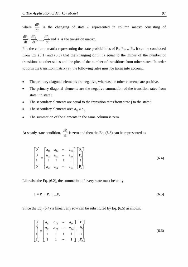
6. The Application of Markov Model 97
where dP
dt is the changing of state P represented in column matrix consisting of
1 2 ndP dP dP, , ....,
dt dt dtand a is the transition matrix.
P is the column matrix representing the state probabilities of P1, P2, …Pn. It can be concluded
from Eq. (6.1) and (6.3) that the changing of P1 is equal to the minus of the number of
transitions to other states and the plus of the number of transitions from other states. In order
to form the transition matrix (a), the following rules must be taken into account.
• The primary diagonal elements are negative, whereas the other elements are positive.
• The primary diagonal elements are the negative summation of the transition rates from
state i to state j.
• The secondary elements are equal to the transition rates from state j to the state i.
• The secondary elements are: ij jia a≠
• The summation of the elements in the same column is zero.
At steady state condition, ndP
dtis zero and then the Eq. (6.3) can be represented as
11 12 1n 1
21 22 2n 2
n1 n2 nn n
a a a P0
a a a P0 =
a a a P0
⋅
L
L
M M M M MM
L
(6.4)
Likewise the Eq. (6.2), the summation of every state must be unity.
1 2 n1 = P + P + ...P (6.5)
Since the Eq. (6.4) is linear, any row can be substituted by Eq. (6.5) as shown.
⋅
=
n
n
n
P
P
P
aaa
aaa
M
L
MMMM
L
L
M
2
1
22221
11211
1111
0
0
(6.6)
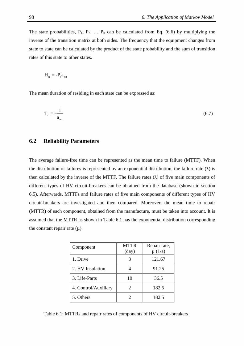
6. The Application of Markov Model 98
The state probabilities, P1, P2, … Pn can be calculated from Eq. (6.6) by multiplying the
inverse of the transition matrix at both sides. The frequency that the equipment changes from
state to state can be calculated by the product of the state probability and the sum of transition
rates of this state to other states.
n n nnH = -P a
The mean duration of residing in each state can be expressed as:
nnn
1T = -
a (6.7)
6.2 Reliability Parameters
The average failure-free time can be represented as the mean time to failure (MTTF). When
the distribution of failures is represented by an exponential distribution, the failure rate (λ) is
then calculated by the inverse of the MTTF. The failure rates (λ) of five main components of
different types of HV circuit-breakers can be obtained from the database (shown in section
6.5). Afterwards, MTTFs and failure rates of five main components of different types of HV
circuit-breakers are investigated and then compared. Moreover, the mean time to repair
(MTTR) of each component, obtained from the manufacture, must be taken into account. It is
assumed that the MTTR as shown in Table 6.1 has the exponential distribution corresponding
the constant repair rate (µ).
Component MTTR (day)
Repair rate, µ (1/a)
1. Drive 3 121.67
2. HV Insulation 4 91.25
3. Life-Parts 10 36.5
4. Control/Auxiliary 2 182.5
5. Others 2 182.5
Table 6.1: MTTRs and repair rates of components of HV circuit-breakers
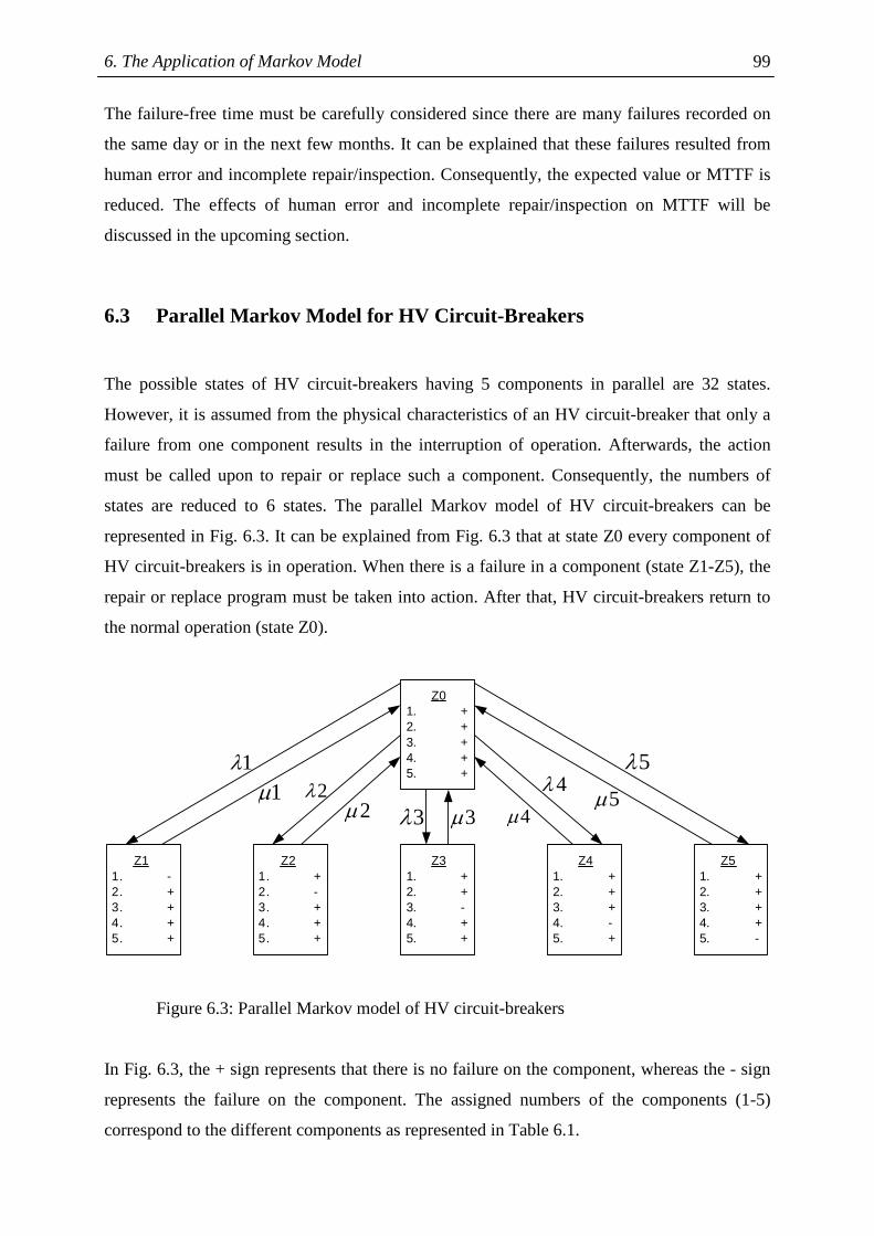
6. The Application of Markov Model 99
The failure-free time must be carefully considered since there are many failures recorded on
the same day or in the next few months. It can be explained that these failures resulted from
human error and incomplete repair/inspection. Consequently, the expected value or MTTF is
reduced. The effects of human error and incomplete repair/inspection on MTTF will be
discussed in the upcoming section.
6.3 Parallel Markov Model for HV Circuit-Breakers
The possible states of HV circuit-breakers having 5 components in parallel are 32 states.
However, it is assumed from the physical characteristics of an HV circuit-breaker that only a
failure from one component results in the interruption of operation. Afterwards, the action
must be called upon to repair or replace such a component. Consequently, the numbers of
states are reduced to 6 states. The parallel Markov model of HV circuit-breakers can be
represented in Fig. 6.3. It can be explained from Fig. 6.3 that at state Z0 every component of
HV circuit-breakers is in operation. When there is a failure in a component (state Z1-Z5), the
repair or replace program must be taken into action. After that, HV circuit-breakers return to
the normal operation (state Z0).
Z01. +2. +3. +4. +5. +
Z11. -2. +3. +4. +5. +
Z21. +2. -3. +4. +5. +
Z31. +2. +3. -4. +5. +
Z41. +2. +3. +4. -5. +
Z51. +2. +3. +4. +5. -
1λ1µ
2µ2λ
3µ3λ 4µ
4λ5λ
5µ
Figure 6.3: Parallel Markov model of HV circuit-breakers
In Fig. 6.3, the + sign represents that there is no failure on the component, whereas the - sign
represents the failure on the component. The assigned numbers of the components (1-5)
correspond to the different components as represented in Table 6.1.

6. The Application of Markov Model 100
6.4 Matrix Approach
The transition rates of the multi-component systems can be easily expressed in the form of a
transition matrix. The primary diagonal elements (i = j) of the matrix are the negative of the
summation of outgoing transition rates of state i. For the secondary diagonal elements, the
element i, j is the transition rate into state i from state j where i ≠ j. The transition matrix of
the parallel Markov model (Fig. 6.3) can be represented as:
0
1
0
12
2
33
4
4 5
5
dP
dtdP
P-(λ1 + λ2 + λ3 + λ4 + λ5) µ1 µ2 µ3 µ4 µ5dtPλ1 -µ1 0 0 0 0dPPλ2 0 -µ2 0 0 0dt = Pλ3 0 0 -µ3 0 0dP
dt Pλ4 0 0 0 -µ4 0dP Pλ5 0 0 0 0 -µ5dtdP
dt
⋅
(6.8)
0 1 2 3 4 5P + P + P + P + P + P = 1 (6.9)
The Eq. (6.9) will be replaced in the Eq. (6.8), thus resulting in the transition matrix, a.
0
1
2
3
4
5
P0 -(λ1 + λ2 + λ3 + λ4 + λ5) µ1 µ2 µ3 µ4 µ5
P0 λ1 -µ1 0 0 0 0
P0 λ2 0 -µ2 0 0 0 =
Pλ3 0 0 -µ3 0 00
Pλ4 0 0 0 -µ4 00
P1 1 1 1 1 11
⋅
(6.10)
The probabilities P0 to P5 of states Z0 to Z5 can be calculated by using Cramer’s rule. The
steady-state availability of HV circuit-breakers is considered as the probability of state Z0. In
addition, the duration of residing in each state can be calculated as follows:
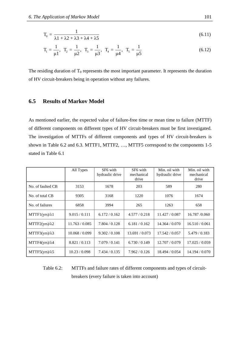
6. The Application of Markov Model 101
0
1T =
λ1 + λ2 + λ3 + λ4 + λ5 (6.11)
1 2 3 4 5
1 1 1 1 1T = , T = , T = , T = , T =
µ1 µ2 µ3 µ4 µ5 (6.12)
The residing duration of T0 represents the most important parameter. It represents the duration
of HV circuit-breakers being in operation without any failures.
6.5 Results of Markov Model
As mentioned earlier, the expected value of failure-free time or mean time to failure (MTTF)
of different components on different types of HV circuit-breakers must be first investigated.
The investigation of MTTFs of different components and types of HV circuit-breakers is
shown in Table 6.2 and 6.3. MTTF1, MTTF2, …, MTTF5 correspond to the components 1-5
stated in Table 6.1
All Types SF6 with hydraulic drive
SF6 with mechanical
drive
Min. oil with hydraulic drive
Min. oil with mechanical
drive
No. of faulted CB 3153 1678 203 589 280
No. of total CB 9305 3168 1220 1076 1674
No. of failures 6858 3994 265 1263 658
MTTF1(yrs)/λ1 9.015 / 0.111 6.172 / 0.162 4.577 / 0.218 11.427 / 0.087 16.787 /0.060
MTTF2(yrs)/λ2 11.763 / 0.085 7.804 / 0.128 6.181 / 0.162 14.364 / 0.070 16.510 / 0.061
MTTF3(yrs)/λ3 10.068 / 0.099 9.302 / 0.108 13.691 / 0.073 17.542 / 0.057 5.479 / 0.183
MTTF4(yrs)/λ4 8.821 / 0.113 7.079 / 0.141 6.730 / 0.149 12.707 / 0.079 17.025 / 0.059
MTTF5(yrs)/λ5 10.23 / 0.098 7.434 / 0.135 7.962 / 0.126 18.494 / 0.054 14.194 / 0.070
Table 6.2: MTTFs and failure rates of different components and types of circuit-
breakers (every failure is taken into account)
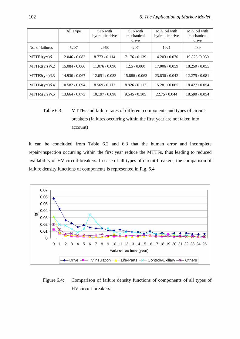
6. The Application of Markov Model 102
All Type SF6 with hydraulic drive
SF6 with mechanical
drive
Min. oil with hydraulic drive
Min. oil with mechanical
drive
No. of failures 5207 2968 207 1021 439
MTTF1(yrs)/λ1 12.046 / 0.083 8.773 / 0.114 7.176 / 0.139 14.203 / 0.070 19.823 /0.050
MTTF2(yrs)/λ2 15.084 / 0.066 11.076 / 0.090 12.5 / 0.080 17.006 / 0.059 18.250 / 0.055
MTTF3(yrs)/λ3 14.930 / 0.067 12.051 / 0.083 15.880 / 0.063 23.830 / 0.042 12.275 / 0.081
MTTF4(yrs)/λ4 10.582 / 0.094 8.569 / 0.117 8.926 / 0.112 15.281 / 0.065 18.427 / 0.054
MTTF5(yrs)/λ5 13.664 / 0.073 10.197 / 0.098 9.545 / 0.105 22.75 / 0.044 18.590 / 0.054
Table 6.3: MTTFs and failure rates of different components and types of circuit-
breakers (failures occurring within the first year are not taken into
account)
It can be concluded from Table 6.2 and 6.3 that the human error and incomplete
repair/inspection occurring within the first year reduce the MTTFs, thus leading to reduced
availability of HV circuit-breakers. In case of all types of circuit-breakers, the comparison of
failure density functions of components is represented in Fig. 6.4
0
0.01
0.02
0.03
0.04
0.05
0.06
0.07
0 1 2 3 4 5 6 7 8 9 10 11 12 13 14 15 16 17 18 19 20 21 22 23 24 25
Failure-free time (year)
f(t)
Drive HV Insulation Life-Parts Control/Auxiliary Others
Figure 6.4: Comparison of failure density functions of components of all types of
HV circuit-breakers

6. The Application of Markov Model 103
It can be seen from Fig. 6.4 that the functions are not perfectly exponentially distributed.
However, the error between the real failure function and exponential function is relatively
small and will not be discussed in this study. The exponential function can be represented as
follows:
-λtf(t) = λ e⋅
The investigation of availability of HV circuit-breakers has been carried out by replacing the
values from Table 6.2 and 6.3 into the Eq. 6.10-6.12. As a result, the probability and duration
of residing at every state can be found. The results of the investigation are represented in
Table 6.4 and 6.5.
All Types SF6 with hydraulic
drive
SF6 with mechanical
drive
Min. oil with hydraulic
drive
Min. oil with mechanical
drive
P0 0.9943 0.9928 0.9930 0.9962 0.9932
P1 0.0009 0.0013 0.0018 0.0007 0.0005
P2 0.0009 0.0014 0.0018 0.0008 0.0007
P3 0.0027 0.0029 0.0020 0.0016 0.0050
P4 0.0006 0.0008 0.0008 0.0004 0.0003
P5 0.0005 0.0007 0.0007 0.0003 0.0004
T0 (year) 1.9763 1.4837 1.3736 2.8818 2.3095
T1 (year) 0.0082 0.0082 0.0082 0.0082 0.0082
T2 (year) 0.0110 0.0110 0.0110 0.0110 0.0110
T3 (year) 0.0274 0.0274 0.0274 0.0274 0.0274
T4 (year) 0.0055 0.0055 0.0055 0.0055 0.0055
T5 (year) 0.0055 0.0055 0.0055 0.0055 0.0055
Table 6.4: Probabilities and durations of residing in each state of different types of
HV circuit-breakers (every failure is taken into account)

6. The Application of Markov Model 104
All Types SF6 with hydraulic
drive
SF6 with mechanical
drive
Min. oil with hydraulic
drive
Min. oil with mechanical
drive
P0 0.9959 0.9947 0.9951 0.9970 0.9962
P1 0.0007 0.0009 0.0011 0.0006 0.0004
P2 0.0007 0.0010 0.0009 0.0006 0.0006
P3 0.0018 0.0023 0.0017 0.0011 0.0022
P4 0.0005 0.0006 0.0006 0.0004 0.0003
P5 0.0004 0.0005 0.0006 0.0002 0.0003
T0 (year) 2.611 1.992 2.004 3.571 3.401
T1 (year) 0.0082 0.0082 0.0082 0.0082 0.0082
T2 (year) 0.0110 0.0110 0.0110 0.0110 0.0110
T3 (year) 0.0274 0.0274 0.0274 0.0274 0.0274
T4 (year) 0.0055 0.0055 0.0055 0.0055 0.0055
T5 (year) 0.0055 0.0055 0.0055 0.0055 0.0055
Table 6.5: Probabilities and durations of residing in each state of different types of
HV circuit-breakers (failures occurring within the first year are not
taken into account)
The duration of residing in state Z0 or the duration that HV circuit-breakers are in operation
without failures can be plotted as bar graph as shown in Fig. 6.5.
It is obvious in Fig. 6.5 that without the consideration of the first-year failures (T02), HV
circuit-breakers stay in operation 32%, 24%, 45%, 24%, and 47% longer in all types, SF6
with hydraulic drive, SF6 with mechanical drive, minimum oil with hydraulic drive and
minimum oil with mechanical drive respectively. It could be implied that the duration of
operation can be prolonged when the effects of human error and incomplete repair/inspection
are reduced. It is obvious from the proportion of increasing duration that HV circuit-breakers
with mechanical drives are subject to human error and incomplete repair/inspection more than
ones with hydraulic drives.

6. The Application of Markov Model 105
0
0.5
1
1.5
2
2.5
3
3.5
4
All Types SF6-hy SF6-me Oil-hy Oil-me
Types of HV circuit-breakers
Dur
atio
n of
res
idin
g in
sta
te Z
0 (y
ear)
T01
T02
Figure 6.5: The durations of residing in state Z0
T01: every failure is considered
T02: failures in the first year are not considered
The steady-state availabilities of different types of HV circuit-breakers are all over 0.99 since
the repair times of components are considerably shorter than their MTTFs. It could be
concluded that as long as the action to repair is as short as mentioned, the availability of HV
circuit-breakers remains high.
As mentioned earlier that there is no distinction between minor and major failures in the
database, state Z0, represented the duration without failures, appears to be shorter than
expectation. Practically, it is beneficial to consider the state Z0 with only the effects of major
failures. Therefore, the relationship between minor and major failures [2] is applied. The
average ratio of minor and major failure is 7.3 mf/MF. This factor is then applied in Eq.
(6.11) to find the durations of residing in state Z0. The durations of residing in state Z0
calculated from only major failures can be represented in Table 6.6 and Fig. 6.6.
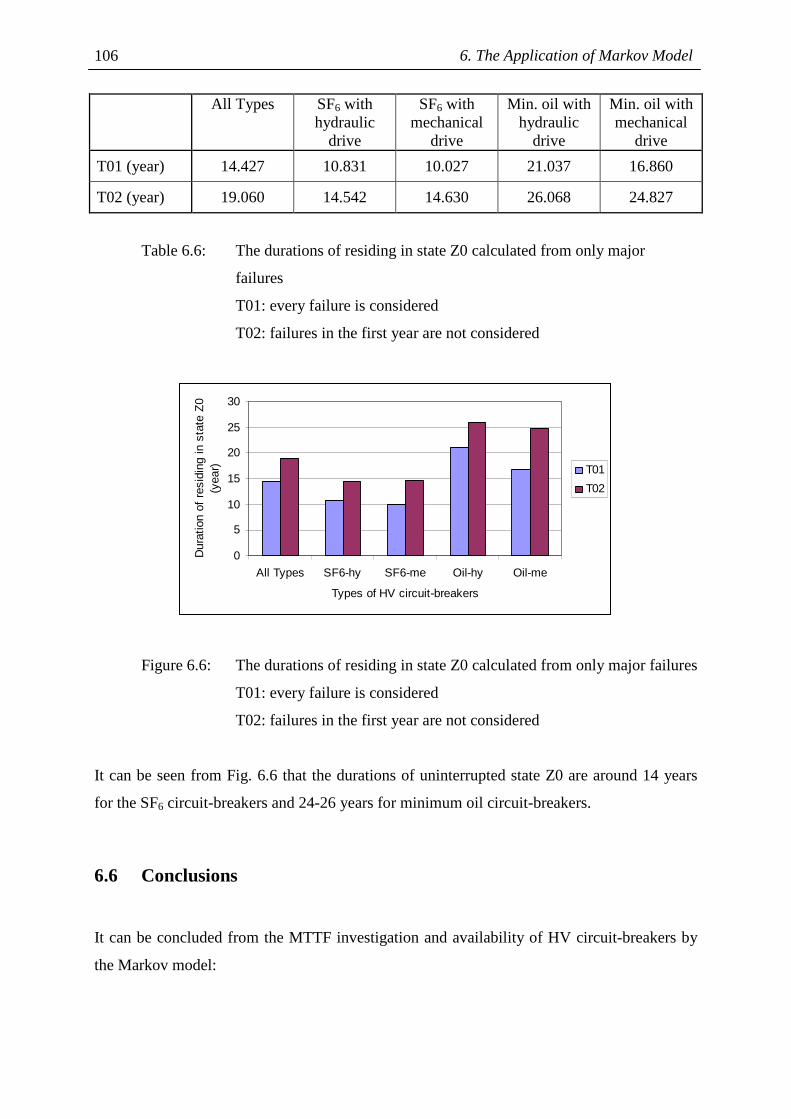
6. The Application of Markov Model 106
All Types SF6 with hydraulic
drive
SF6 with mechanical
drive
Min. oil with hydraulic
drive
Min. oil with mechanical
drive
T01 (year) 14.427 10.831 10.027 21.037 16.860
T02 (year) 19.060 14.542 14.630 26.068 24.827
Table 6.6: The durations of residing in state Z0 calculated from only major
failures
T01: every failure is considered
T02: failures in the first year are not considered
0
5
10
15
20
25
30
All Types SF6-hy SF6-me Oil-hy Oil-me
Types of HV circuit-breakers
Dur
atio
n of
res
idin
g in
sta
te Z
0 (y
ear) T01
T02
Figure 6.6: The durations of residing in state Z0 calculated from only major failures
T01: every failure is considered
T02: failures in the first year are not considered
It can be seen from Fig. 6.6 that the durations of uninterrupted state Z0 are around 14 years
for the SF6 circuit-breakers and 24-26 years for minimum oil circuit-breakers.
6.6 Conclusions
It can be concluded from the MTTF investigation and availability of HV circuit-breakers by
the Markov model:

6. The Application of Markov Model 107
• The investigation of all types of HV circuit-breakers, representing the largest studied
population, shows that HV insulation has the longest MTTF, whereas the
control/auxiliary component has the shortest MTTF.
• The populations of SF6 circuit-breakers with hydraulic drives and SF6 circuit-breakers
with mechanical drives are very different. Therefore, it is difficult to make conclusions as
to the MTTF. However, it is obvious from Table 6.2 that the proportion of faulted circuit-
breakers to total circuit-breakers in the same category represents the overall reliability.
More than half of the population of SF6 circuit-breakers with hydraulic drives had been
exposed to failures, whereas only 16 % of the population of SF6 circuit-breakers with
mechanical drives had experienced failures.
• The mechanical drive has longer MTTF than the hydraulic drive which is in accordance
with practical experience.
• The control/auxiliary components of minimum oil circuit-breakers have longer MTTF
than control/auxiliary components of SF6 circuit-breakers due to less complicated
control/auxiliary in minimum oil circuit-breakers.
• It can be seen from Table 6.2 and 6.3 that without the consideration of failures in the first
year, the MTTFs of components can be increased up to 47 %. It is recommended that
repair/inspection must be carefully carried out in order to prevent the following failures
occurring in the same year.
• Components of minimum oil circuit-breakers have longer MTTFs than components of
SF6 circuit-breakers. However, it must be paid attention that the database of minimum oil
circuit-breakers is longer than SF6 circuit-breakers. The record time of minimum oil
circuit-breakers is around 50 years, whereas the record time of SF6 circuit-breakers is
only 30 years.
• The failure density functions of components are roughly exponentially distributed. In
other words, this exponential distribution corresponds to random failures. Hence, the
preventive or time-based maintenance cannot extend MTTF or reduce the failure rate. In
order to extend MTTF, the predictive or condition-based maintenance must be
introduced.

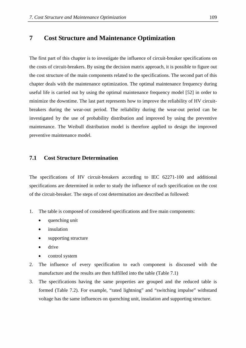
7. Cost Structure and Maintenance Optimization 109
7 Cost Structure and Maintenance Optimization
The first part of this chapter is to investigate the influence of circuit-breaker specifications on
the costs of circuit-breakers. By using the decision matrix approach, it is possible to figure out
the cost structure of the main components related to the specifications. The second part of this
chapter deals with the maintenance optimization. The optimal maintenance frequency during
useful life is carried out by using the optimal maintenance frequency model [52] in order to
minimize the downtime. The last part represents how to improve the reliability of HV circuit-
breakers during the wear-out period. The reliability during the wear-out period can be
investigated by the use of probability distribution and improved by using the preventive
maintenance. The Weibull distribution model is therefore applied to design the improved
preventive maintenance model.
7.1 Cost Structure Determination
The specifications of HV circuit-breakers according to IEC 62271-100 and additional
specifications are determined in order to study the influence of each specification on the cost
of the circuit-breaker. The steps of cost determination are described as followed:
1. The table is composed of considered specifications and five main components:
• quenching unit
• insulation
• supporting structure
• drive
• control system
2. The influence of every specification to each component is discussed with the
manufacture and the results are then fulfilled into the table (Table 7.1)
3. The specifications having the same properties are grouped and the reduced table is
formed (Table 7.2). For example, “rated lightning” and “switching impulse” withstand
voltage has the same influences on quenching unit, insulation and supporting structure.
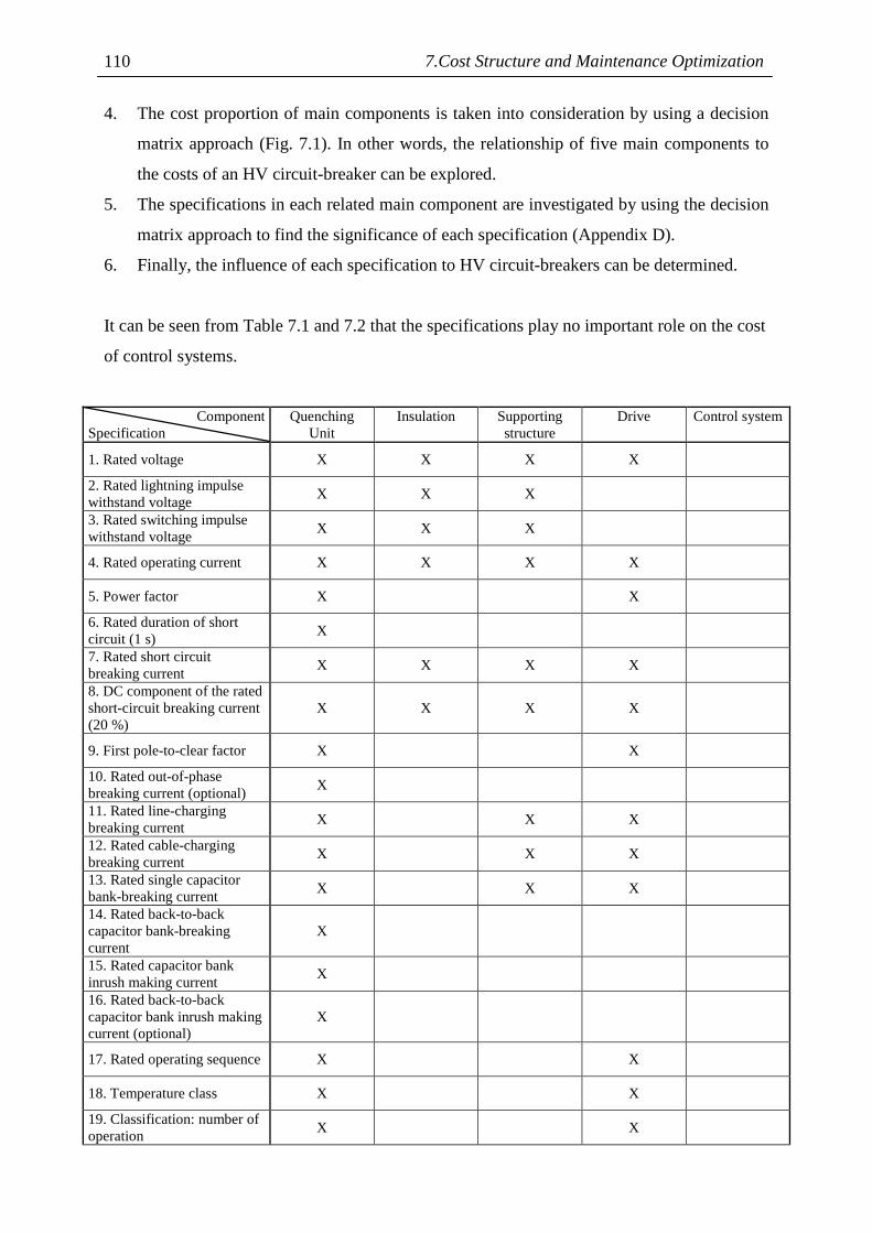
7.Cost Structure and Maintenance Optimization 110
4. The cost proportion of main components is taken into consideration by using a decision
matrix approach (Fig. 7.1). In other words, the relationship of five main components to
the costs of an HV circuit-breaker can be explored.
5. The specifications in each related main component are investigated by using the decision
matrix approach to find the significance of each specification (Appendix D).
6. Finally, the influence of each specification to HV circuit-breakers can be determined.
It can be seen from Table 7.1 and 7.2 that the specifications play no important role on the cost
of control systems.
Component Specification
Quenching Unit
Insulation Supporting structure
Drive Control system
1. Rated voltage X X X X
2. Rated lightning impulse withstand voltage
X X X
3. Rated switching impulse withstand voltage
X X X
4. Rated operating current X X X X
5. Power factor X X
6. Rated duration of short circuit (1 s)
X
7. Rated short circuit breaking current
X X X X
8. DC component of the rated short-circuit breaking current (20 %)
X X X X
9. First pole-to-clear factor X X
10. Rated out-of-phase breaking current (optional)
X
11. Rated line-charging breaking current
X X X
12. Rated cable-charging breaking current
X X X
13. Rated single capacitor bank-breaking current
X X X
14. Rated back-to-back capacitor bank-breaking current
X
15. Rated capacitor bank inrush making current
X
16. Rated back-to-back capacitor bank inrush making current (optional)
X
17. Rated operating sequence X X
18. Temperature class X X
19. Classification: number of operation
X X
7. Cost Structure and Maintenance Optimization 111
Component Specification
Quenching Unit
Insulation Supporting structure
Drive Control system
20. Earthquake level X X X
21. Bending strength X X
22. Pollution level X
23. Overvoltage across CB X X
24. Rate of Rise of Recovery Voltage (RRRV)
X X
25. Short-line faults X
Table 7.1: The influence of specifications to the components
Component Specification
Quenching Unit
Insulation Supporting structure
Drive Control system
1. Rated voltage X X X X
2. Rated lightning and switching impulse withstand voltage
X X X
3. Rated operating current X X X X
4. Rated duration of short circuit (1 s)
X
5. Rated short circuit breaking current and DC component
X X X X
6. First pole-to-clear factor X X
7. Rated out-of-phase breaking current (optional)
X
8. Rated line-charging breaking current
X X X
9. Rated capacitor bank inrush making current
X
10. Rated operating sequence X X
11. Temperature class X X
12. Classification: number of operation
X X
13. Earthquake level X X X
14. Bending strength X X
15. Pollution level X
16. Rate of Rise of Recovery Voltage (RRRV)
X X
Table 7.2: The influence of specifications to the components (reduced version)
7.Cost Structure and Maintenance Optimization 112
Nr. Criteria 1 2 3 4 5 Sum WF/%1 Quenching unit 0 4 5 2 5 16 26.72 Insulation 2 0 5 3 5 15 25.03 Supporting structure 1 1 0 1 4 7 11.74 Drive 4 3 5 0 5 17 28.35 Control System 1 1 2 1 0 5 8.3
60 100.0
Figure 7.1: The decision matrix of five main components
Influence evaluation: 1: very small 4: strong
2: small 5: very strong
3: similar
By using this decision matrix approach, Fig. 7.1, every parameter is compared with each other
with different degrees of significance. For example, the quenching unit compared with the
insulation has stronger influence on the costs. Therefore, the number 4 is placed in the first
row and the second column. On the other hand, the quenching unit compared with drive has
smaller influence on the costs. The number 2 is then placed in the first row and the fourth
column. The upper triangle of the matrix (above the primary diagonal axis) must be
considered. The lower triangle of the matrix (below the primary diagonal axis) is justified by
reversion of the investigation of the above triangle. For example, the insulation compared
with the quenching unit has smaller influence on the costs. The number 2 is then placed in the
second row and the first column. After the whole decision matrix is completed, the proportion
of every main component can be found. The proportion distribution of main components to
the costs of HV circuit-breakers is represented in Fig. 7.2
Insulation25%
Supporting structure
12%
Drive28%
Quenching unit27%
Control system8%
Figure 7.2: The proportion distribution of five main components to the cost of
HV circuit-breakers

7. Cost Structure and Maintenance Optimization 113
It is seen from Fig. 7.2 that the drive or the operating mechanism plays the most important
role on the total cost followed by the quenching unit, the insulation and the supporting
structure.
The specifications of each component represented in Table 7.2 are considered one by one by
using the decision matrix in order to find the proportions of specifications (Appendix D). The
proportions of specifications with respect to each component can be represented as web
diagrams in Fig. 7.3.
0
5
10
15
0
5
10
15
20
25
0
5
10
15
20
25
0
2
4
6
8
10
12
(a) Quenching unit (b) Insulation
(c) Supporting structure (d) Drive
12
3
4
5
6
8 7
9
10
11
12
161
2
3
513
14
15
1
2
3
58
13
14
1
3
5
6
8
1011
12
13
16
% %
% %
Figure 7.3: Web diagrams of the circuit-breaker specifications with respect to each
component (The numbers at the perimeter of the circle correspond to
specifications represented in Table. 7.2)

7.Cost Structure and Maintenance Optimization 114
For instance, the proportion of rated voltage (no. 1) to the cost of the quenching unit is 10%,
while the proportion of rated line charging (no. 8) to the cost of the quenching unit is only
3.3%. In case of the insulation, rated lightning and switching impulse withstand voltage (no.
2) accounts for the highest proportion (20 %).
Component
Specification
Quenching Unit
Insulation
Supporting structure
Drive
Total
1. Rated voltage 2.7 % 4.0 % 2.3 % 4.1 % 13.1 %
2. Rated lightning and switching impulse withstand voltage
2.1 % 5.0 % 2.6 % 9.7 %
3. Rated operating current 2.5 % 2.0 % 0.8 % 1.6 % 6.9 %
4. Rated duration of short circuit (1 s) 1.4 % 1.4 %
5. Rated short circuit breaking current and DC component
3.1 % 3.6 % 2.2 % 3.9 % 12.8 %
6. First pole-to-clear factor 1.9 % 2.2 % 4.1 %
7. Rated out-of-phase breaking current (optional) 1.6 % 1.6 %
8. Rated line-charging , cable-charging and capacitor bank breaking current
0.9 % 0.7 % 1.2 % 2.8 %
9. Rated capacitor bank inrush making current 1.8 % 1.8 %
10. Rated operating sequence 2.3 % 3.7 % 6.0 %
11. Temperature class 2.5 % 3.9 % 6.4 %
12. Classification: number of operation 2.1 % 3.0 % 5.1 %
13. Earthquake level 3.2 % 1.7 % 2.0 % 6.9 %
14. Bending strength 3.6 % 1.7 % 5.3 %
15. Pollution level 3.6 % 3.6 %
16. Rate of Rise of Recovery Voltage (RRRV) 2.1 % 2.4 % 4.5 %
Total 27 % 25 % 12 % 28 % 92 %
Table 7.3: The proportions of specifications to the main components
(without control system)
The proportions of specifications related to the circuit-breaker are shown in Table 7.3. The
whole table of which the control system (8 %) is not included represents 92 %. It can be
expressed in terms of pie chart in Fig. 7.4. The influence of specifications on the cost of the

7. Cost Structure and Maintenance Optimization 115
circuit-breaker is as shown in Fig. 7.4 is valuable for the circuit-breaker designers to design
the optimal and cost-effective HV circuit-breakers.
14, 5.3
15, 3.6
16, 4.51, 13.1
2, 9.7
3, 6.9
4, 1.4
5, 12.8
6, 4.17, 1.68, 2.8
10, 6
11, 6.4
12, 5.1
13, 6.9
9, 1.8
Figure 7.4: The proportions of specifications to the cost of HV circuit-breaker
The most and least important specifications to the cost of circuit-breakers can be summarized
in Table 7.4
The most important specifications
% The least important specifications
%
1. Rated voltage 13.1 Rated duration of short-circuit
1.4
2. Rated short-circuit breaking current
12.8 Rated out-of-phase breaking current
1.6
3. Rated lightning and switching impulse withstand voltage
9.7 Rated capacitor bank inrush making current
1.8
Table 7.4 The most and least important influences on the cost of circuit-breakers
7.2 Maintenance Optimization
In the first part of this section, the optimal maintenance frequency during the useful lifetime is
calculated by using the optimal maintenance frequency model and failure statistics during
1991-2000 [37]. The optimal maintenance frequency of different types of HV circuit-breakers

7.Cost Structure and Maintenance Optimization 116
at different voltage levels had been investigated. The second part of this section concerns with
the improvement of maintenance strategy during the wear-out period. The wear-out behaviour
of HV circuit-breakers is simulated by a Weibull distribution. The integration of different
preventive maintenance models represents the improvement of reliability of HV circuit-
breakers.
7.2.1 Optimal Maintenance Frequency
The equipment of HV circuit-breakers breaks down from time to time. In order to reduce the
breakdowns, periodic maintenance must be implemented. However, the maintenance might
result in the system downtime. More frequent maintenance could reduce the downtime due to
system failures but increase the downtime due to maintenance. The principle of optimal
maintenance frequency in order to minimize the downtime can be expressed in Fig. 7.5.
Maintenance frequency (n)
To
tal d
ow
ntim
e (D
)
Total downtime D(n)
Downtime due to maintenance
Downtime due to system failures
Figure 7.5: Optimal maintenance frequency: Minimization of downtime
It is obvious from Fig. 7.5 that the total downtime, D(n), is the summation of downtime due to
maintenance (DM) and downtime due to system failures. The downtime due to system failures
can be mentioned as downtime due to repairs (DR).
D(n) = DR + DM = λ(n) n
+ µ i
(7.1)

7. Cost Structure and Maintenance Optimization 117
where:
Parameter Equation Remark
λ(n) 1/mean time to failure (MTTF) Failure rate or number of repairs per unit time
µ 1/mean time to repair (MTTR) Repair rate
n Number of periodic maintenance per unit time
i 1/mean time to maintenance (MTTM) Maintenance rate
DR λ(n)/µ Downtime due to repair
DM n/i Downtime due to maintenance
In order to find the optimal maintenance frequency, the derivative of downtime is applied as
followed.
'dD(n) λ (n) 1
= + = 0dn µ i
(7.2)
It is assumed that the failure rate varies inversely with the number of periodical maintenance.
k is the arrival rate of failure per unit time when one periodical maintenance is made per unit
time.
k
λ(n) = n
'2
kλ (n) = -
n (7.3)
From Eq. (7.2) and (7.3), the optimal maintenance frequency, n, can be found. The value n is
the number of optimal maintenance frequency per year.
i k MTTR k
n = = µ MTTM
⋅ ⋅ (7.4)
From the database, it is estimated that the periodical minor and major maintenance of HV
circuit-breakers are carried out every 4 and 7 years respectively. It is assumed that the minor
maintenance is related to the minor failures and the major maintenance is related to major
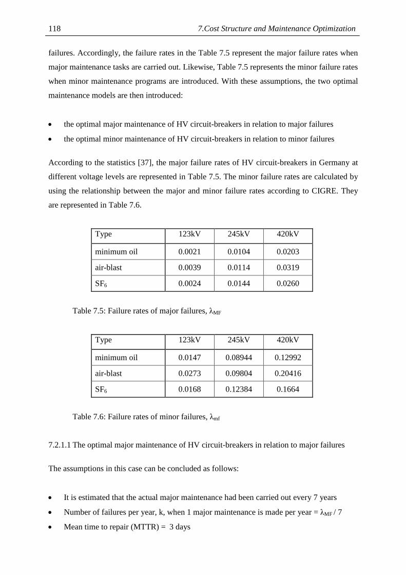
7.Cost Structure and Maintenance Optimization 118
failures. Accordingly, the failure rates in the Table 7.5 represent the major failure rates when
major maintenance tasks are carried out. Likewise, Table 7.5 represents the minor failure rates
when minor maintenance programs are introduced. With these assumptions, the two optimal
maintenance models are then introduced:
• the optimal major maintenance of HV circuit-breakers in relation to major failures
• the optimal minor maintenance of HV circuit-breakers in relation to minor failures
According to the statistics [37], the major failure rates of HV circuit-breakers in Germany at
different voltage levels are represented in Table 7.5. The minor failure rates are calculated by
using the relationship between the major and minor failure rates according to CIGRE. They
are represented in Table 7.6.
Type 123kV 245kV 420kV
minimum oil 0.0021 0.0104 0.0203
air-blast 0.0039 0.0114 0.0319
SF6 0.0024 0.0144 0.0260
Table 7.5: Failure rates of major failures, λMF
Type 123kV 245kV 420kV
minimum oil 0.0147 0.08944 0.12992
air-blast 0.0273 0.09804 0.20416
SF6 0.0168 0.12384 0.1664
Table 7.6: Failure rates of minor failures, λmf
7.2.1.1 The optimal major maintenance of HV circuit-breakers in relation to major failures
The assumptions in this case can be concluded as follows:
• It is estimated that the actual major maintenance had been carried out every 7 years
• Number of failures per year, k, when 1 major maintenance is made per year = λMF / 7
• Mean time to repair (MTTR) = 3 days
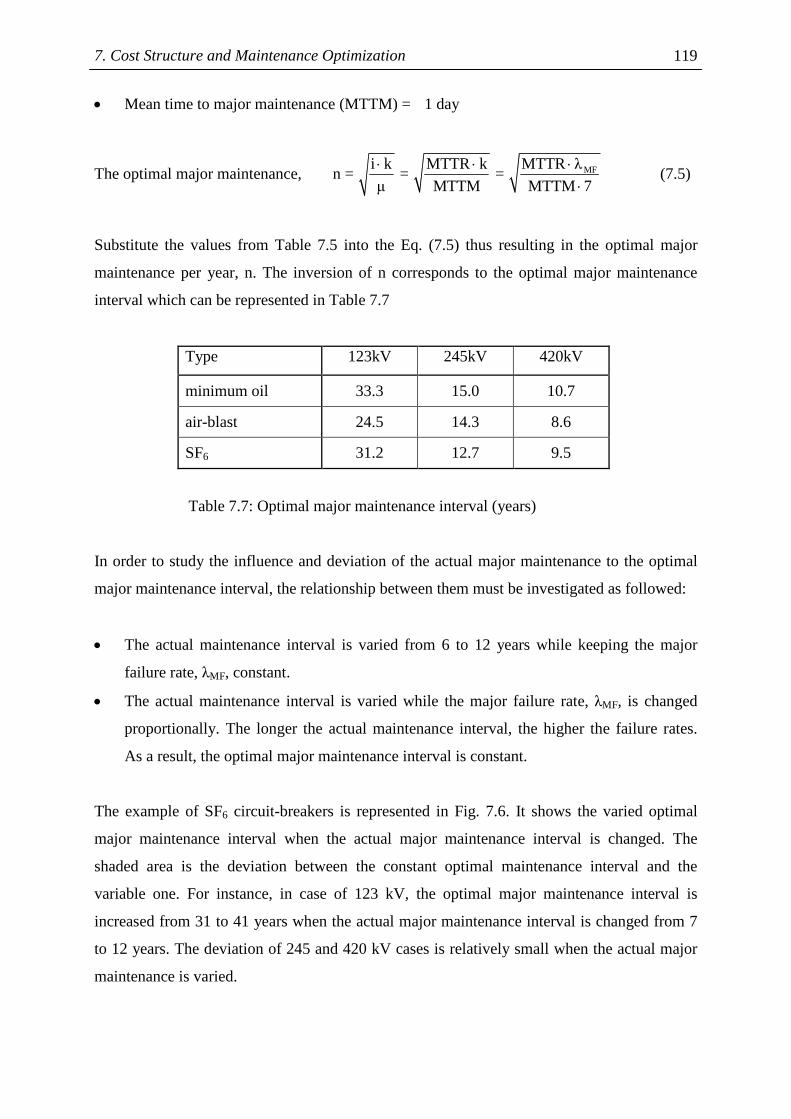
7. Cost Structure and Maintenance Optimization 119
• Mean time to major maintenance (MTTM) = 1 day
The optimal major maintenance, MFi k MTTR k MTTR λn = = =
µ MTTM MTTM 7
⋅ ⋅ ⋅
⋅ (7.5)
Substitute the values from Table 7.5 into the Eq. (7.5) thus resulting in the optimal major
maintenance per year, n. The inversion of n corresponds to the optimal major maintenance
interval which can be represented in Table 7.7
Type 123kV 245kV 420kV
minimum oil 33.3 15.0 10.7
air-blast 24.5 14.3 8.6
SF6 31.2 12.7 9.5
Table 7.7: Optimal major maintenance interval (years)
In order to study the influence and deviation of the actual major maintenance to the optimal
major maintenance interval, the relationship between them must be investigated as followed:
• The actual maintenance interval is varied from 6 to 12 years while keeping the major
failure rate, λMF, constant.
• The actual maintenance interval is varied while the major failure rate, λMF, is changed
proportionally. The longer the actual maintenance interval, the higher the failure rates.
As a result, the optimal major maintenance interval is constant.
The example of SF6 circuit-breakers is represented in Fig. 7.6. It shows the varied optimal
major maintenance interval when the actual major maintenance interval is changed. The
shaded area is the deviation between the constant optimal maintenance interval and the
variable one. For instance, in case of 123 kV, the optimal major maintenance interval is
increased from 31 to 41 years when the actual major maintenance interval is changed from 7
to 12 years. The deviation of 245 and 420 kV cases is relatively small when the actual major
maintenance is varied.

7.Cost Structure and Maintenance Optimization 120
0
5
10
15
20
25
30
35
40
45
6 7 8 9 10 11 12
Major maintenance interval (year)
Op
tima
l mai
nte
na
nce
inte
rval
(ye
ar)
123 kV
245 kV
420 kV
Actual major maintenance interval (year)
Opt
ima
l ma
jor
mai
nten
ance
inte
rval
(ye
ar)
Figure 7.6: The deviation of optimal major maintenance interval with respect to
major maintenance interval (SF6 circuit-breakers)
7.2.1.2 The optimal minor maintenance of HV circuit-breakers in relation to minor failures
The assumptions in this case can be summarized as follows:
• It is estimated that the actual minor maintenance is carried out every 4 years
• Number of failures per year, k, when 1 minor maintenance is made per year = λmf / 4
• Mean time to repair (MTTR) = 1 day
• Mean time to minor maintenance (MTTm) = 0.5 day
The optimal minor maintenance, mfi k MTTR k MTTR λn = = =
µ MTTm MTTm 4
⋅ ⋅ ⋅
⋅ (7.6)
Substitute the values from Table 7.6 into the Eq. (7.6) thus resulting in the optimal minor
maintenance per year, n. The inversion of n corresponds to the optimal minor maintenance
interval which can be represented in Table 7.8

7. Cost Structure and Maintenance Optimization 121
Type 123kV 245kV 420kV
minimum oil 11.7 4.7 3.9
air-blast 8.6 4.5 3.1
SF6 10.9 4.0 3.5
Table 7.8: Optimal minor maintenance interval (years)
The influence and deviation of actual minor maintenance interval to the optimal minor
maintenance interval can be performed in the same way as major maintenance. The actual
minor maintenance interval is varied from 3 to 9 years.
Fig. 7.7 represents the example of SF6 circuit-breakers. The deviation between the constant
optimal maintenance interval and the variable one is shown in the shaded area. In case of 123
kV, it can be seen that the optimal minor maintenance interval is varied from around 11 to 16
years when the actual minor maintenance is changed from 4 to 9 years. The deviation in case
of 245 and 420 kV is smaller than 123 kV.
0
2
4
6
8
10
12
14
16
18
3 4 5 6 7 8 9
Actual minor maintenance interval
Op
tim
al m
ino
r m
ain
ten
ance
inte
rval
Opt
imal
min
or m
aint
ena
nce
inte
rva
l (ye
ar)
Actual minor maintenance interval (year)
123 kV
245 kV
420 kV
Figure 7.7: The deviation of optimal minor maintenance interval with respect to
minor maintenance interval (SF6 circuit-breakers)
The optimal minor and major maintenance of different types of HV circuit-breakers at
different voltage levels can be concluded in Table 7.9.
7.Cost Structure and Maintenance Optimization 122
123 kV 245 kV 420 kV
minor maintenance
(years)
major maintenance
(years)
minor maintenance
(years)
major maintenance
(years)
minor maintenance
(years)
major maintenance
(years)
minimum oil 11.7 33.3 4.7 15.0 3.9 10.7
air-blast 8.6 24.5 4.5 14.3 3.1 8.6
SF6 10.9 31.2 4.0 12.7 3.5 9.5
Table 7.9: The optimal minor and major maintenance intervals of HV circuit-breakers
It can be concluded from Table 7.9 that:
• Since 123 kV-HV circuit-breakers had been subject to relatively small failures, the actual
minor and major maintenance intervals of 4 and 7 years respectively are too frequent.
The optimal minor maintenance interval should be around 8 – 12 years depending on
types of circuit-breakers. The optimal major maintenance programs of 123kV-HV
circuit-breakers should be performed every 24 – 33 years.
• The minor failure rates of 245 kV-HV circuit-breakers are relatively high. The optimal
minor maintenance intervals in this case are around 4-5 years. The optimal major
maintenance interval should be extended from 7 years to 14 years in this voltage level.
• In case of 420 kV-HV circuit-breakers, the optimal minor maintenance interval should be
performed every 3-4 years, whereas the optimal major maintenance programs should be
carried out every 8-10 years.
• It can be seen from the calculation that with the optimal minor and major maintenance
programs, the numbers of maintenance are reduced and the systems operate at the
minimum downtime.
7.3 Reliability under Preventive Maintenance
7.3.1 Concepts of Preventive Maintenance
The preventive maintenance programs can reduce the effect of aging or wear-out resulting in
the extending of lifetime of HV circuit-breakers. It is assumed that after preventive

7. Cost Structure and Maintenance Optimization 123
maintenance, the reliability of HV circuit-breakers is restored to the original condition. The
reliability of HV circuit-breakers with preventive maintenance is represented as
mR (t) = R(t) for 0 t < T≤ (7.7)
mR (t) = R(T) R(t - T)⋅ for T t < 2T≤ (7.8)
Rm(t) in Eq. (7.7) is the reliability without maintenance and T is the interval to perform
preventive maintenance. It is seen in Eq. (7.8) that the preventive maintenance is performed at
time T, where R(T) is the survivor function until the first preventive maintenance and R(t - T)
is the survivor function at additional time (t - T). HV circuit-breakers are restored to their
original state at time T. The Eq. (7.8) can be generally expressed as:
nmR (t) = R(T) R(t - nT)⋅ (7.9)
where nT t < (n+1)T≤ , n = 1, 2, 3, …
R(T)n is the survivor function of surviving n maintenance intervals and R(t - nT) is the
survivor function of additional time (t - nT) after the last preventive maintenance. It is noted
that the preventive maintenance cannot be applied during the useful life having exponential
distribution. In other words, the preventive maintenance is not applicable under constant
failure rate condition as represented below.
-λtR(t) = e
nmR (t) = R(T) R(t - nT)⋅
-λT n -λ(t - nT)mR (t) = (e ) (e )⋅
-λnT -λt λnT -λtmR (t) = e e e = e⋅ ⋅
It can be seen that the preventive maintenance cannot increase the reliability under constant
failure rate condition.

7.Cost Structure and Maintenance Optimization 124
7.3.2 Application of Preventive Maintenance to HV Circuit-Breakers
It must be noted that the preventive maintenance is effective in the wear-out period in order to
increase their reliabilities. After preventive maintenance is performed, the reliability of HV
circuit-breakers is restored to the original condition. The equation of reliability of HV circuit-
breakers with preventive maintenance is represented as followed:
β β
m
T t - nTR (t) = exp -n exp -
α α
⋅
nT t (n+1)T≤ < (7.10)
where n: the number of preventive maintenance before the considered period of time
T: interval of time between preventive maintenance
The case of all types of HV circuit-breakers had been used to show the application of
preventive maintenance. The failure rate distribution extracted from the failure database of all
types of HV circuit-breakers is depicted in Fig. 7.8. The failure distribution represents the
relative failure rate of the first failures of circuit-breakers. As a result, the trend of failure
development during the lifetime can be investigated.
0
0.1
0.2
0.3
0.4
0.5
0.6
0 2 4 6 8 10 12 14 16 18 20 22 24 26 28 30 32 34
Year
Fai
lure
rat
e
Figure 7.8: The relative failure rate distribution of all types of circuit-breakers

7. Cost Structure and Maintenance Optimization 125
It can be seen from Fig. 7.8 that the failure rate is relatively constant until the 20th year. From
the 20th year, the failure rate is increased and it is assumed that this is the Weibull distribution.
From the 30th year, the distribution is fluctuated and not precise because of small numbers of
samples. Therefore, the parameters of Weibull distribution are determined by using the failure
distribution during the 20th - 30th year.
From the failure database, it is found that the maintenance and overhaul are carried out every
7 and 12 years respectively. As discussed earlier, the preventive maintenance cannot increase
the reliability when the failure rate is constant (the first 20 years). The investigation then starts
at the 20th year and it is assumed that the reliability of circuit-breakers starts at unity in this
year in order to simplify the explanation of reliability under preventive maintenance. By using
the MATLAB curve-fitting program, it is possible to find the Weibull parameters α and β
which are equal to 10 and 4 respectively. The reliability with the preventive maintenance can
be represented as:
4 4
m
T t - nTR (t) = exp -n exp -
10 10
⋅
(7.11)
With the Eq. (7.11), the maintenance interval T is varied in order to study the effects of
preventive maintenance to the reliability of HV circuit-breakers. The example of maintenance
interval of 7 years is illustrated in Fig. 7.9. The effects of different preventive maintenance in
terms of the maintenance frequency to the reliability are represented in Fig. 7.10.
It is obvious from Fig. 7.9 that the preventive maintenance has the same distribution as the
original reliability distribution but it will be restored to the original condition at the specified
maintenance period. When the preventive maintenance is implemented into the original
reliability distribution, the decreasing reliability over time can be slowed down. As a result,
the lifetime of the HV circuit-breaker can be extended.
The more frequent preventive maintenance results in the more effective extension of the
lifetime. However, the cost of frequent maintenance during the wear-out period might be
more expensive than the cost of replacing with the new circuit-breakers. Therefore, the
optimal maintenance during wear-out period must be calculated.
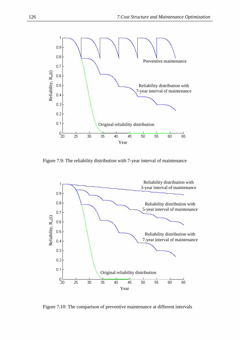
7.Cost Structure and Maintenance Optimization 126
Original reliability distribution
Preventive maintenance
Reliability distribution with 7-year interval of maintenance
Year
Rel
iabi
lity,
Rm(t)
Figure 7.9: The reliability distribution with 7-year interval of maintenance
Original reliability distribution
Reliability distribution with 7-year interval of maintenance
Reliability distribution with 5-year interval of maintenance
Reliability distribution with 3-year interval of maintenance
Re
liab
ility
, Rm(t
)
Year
Figure 7.10: The comparison of preventive maintenance at different intervals
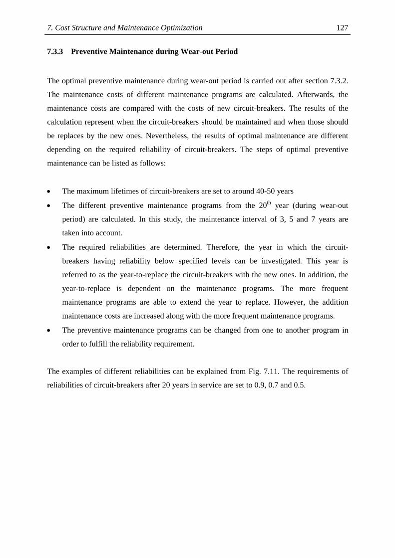
7. Cost Structure and Maintenance Optimization 127
7.3.3 Preventive Maintenance during Wear-out Period
The optimal preventive maintenance during wear-out period is carried out after section 7.3.2.
The maintenance costs of different maintenance programs are calculated. Afterwards, the
maintenance costs are compared with the costs of new circuit-breakers. The results of the
calculation represent when the circuit-breakers should be maintained and when those should
be replaces by the new ones. Nevertheless, the results of optimal maintenance are different
depending on the required reliability of circuit-breakers. The steps of optimal preventive
maintenance can be listed as follows:
• The maximum lifetimes of circuit-breakers are set to around 40-50 years
• The different preventive maintenance programs from the 20th year (during wear-out
period) are calculated. In this study, the maintenance interval of 3, 5 and 7 years are
taken into account.
• The required reliabilities are determined. Therefore, the year in which the circuit-
breakers having reliability below specified levels can be investigated. This year is
referred to as the year-to-replace the circuit-breakers with the new ones. In addition, the
year-to-replace is dependent on the maintenance programs. The more frequent
maintenance programs are able to extend the year to replace. However, the addition
maintenance costs are increased along with the more frequent maintenance programs.
• The preventive maintenance programs can be changed from one to another program in
order to fulfill the reliability requirement.
The examples of different reliabilities can be explained from Fig. 7.11. The requirements of
reliabilities of circuit-breakers after 20 years in service are set to 0.9, 0.7 and 0.5.

7.Cost Structure and Maintenance Optimization 128
Original reliability distribution
Reliability distribution with 7-year interval of maintenance
Reliability distribution with 5-year interval of maintenance
Reliability distribution with 3-year interval of maintenance
Year
Rel
iabi
lity,
Rm(t
)
Figure 7.11: The requirements of reliabilities and the different maintenance programs
It can be concluded from the Fig. 7.11:
• When the reliability of circuit-breakers of 0.9 is desired, the 7-year interval maintenance
cannot prolong the time to replace, since the time to replace (at the 26th year) takes place
before the implementation of preventive maintenance. The time to replace can be
prolonged to 29 years when the 5-year interval maintenance is applied. The time to
replace can be even extended to 60 years, when the 3-year interval maintenance is
implemented. However, the maximum lifetime is limited to 50 years and the 3-year
maintenance might not be cost-effective.
• When the reliability of circuit-breakers of 0.7 is required, the original distribution shows
the time to replace of 28 years. With the 7-year interval maintenance, the time to replace
can be extended to 33 years. The time to replace can be prolonged to 49 years with the 5-
year interval maintenance. The 3-year maintenance program is not considered, since the
lifetimes of circuit-breakers are however limited to 50 years.
• When the reliability of 0.5 is acceptable, the original distribution represents the time to
replace of 29 years. With the 7-year interval maintenance, the time to replace can be
extended to 41 years. The 3 and 5-year interval maintenance programs are not taken into
account, since the time to replace is beyond the maximum lifetime.
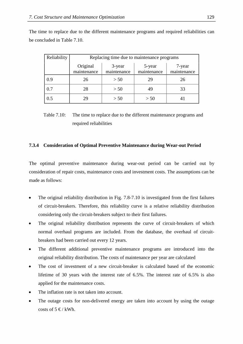
7. Cost Structure and Maintenance Optimization 129
The time to replace due to the different maintenance programs and required reliabilities can
be concluded in Table 7.10.
Replacing time due to maintenance programs Reliability
Original maintenance
3-year maintenance
5-year maintenance
7-year maintenance
0.9 26 > 50 29 26
0.7 28 > 50 49 33
0.5 29 > 50 > 50 41
Table 7.10: The time to replace due to the different maintenance programs and
required reliabilities
7.3.4 Consideration of Optimal Preventive Maintenance during Wear-out Period
The optimal preventive maintenance during wear-out period can be carried out by
consideration of repair costs, maintenance costs and investment costs. The assumptions can be
made as follows:
• The original reliability distribution in Fig. 7.8-7.10 is investigated from the first failures
of circuit-breakers. Therefore, this reliability curve is a relative reliability distribution
considering only the circuit-breakers subject to their first failures.
• The original reliability distribution represents the curve of circuit-breakers of which
normal overhaul programs are included. From the database, the overhaul of circuit-
breakers had been carried out every 12 years.
• The different additional preventive maintenance programs are introduced into the
original reliability distribution. The costs of maintenance per year are calculated
• The cost of investment of a new circuit-breaker is calculated based of the economic
lifetime of 30 years with the interest rate of 6.5%. The interest rate of 6.5% is also
applied for the maintenance costs.
• The inflation rate is not taken into account.
• The outage costs for non-delivered energy are taken into account by using the outage
costs of 5 € / kWh.
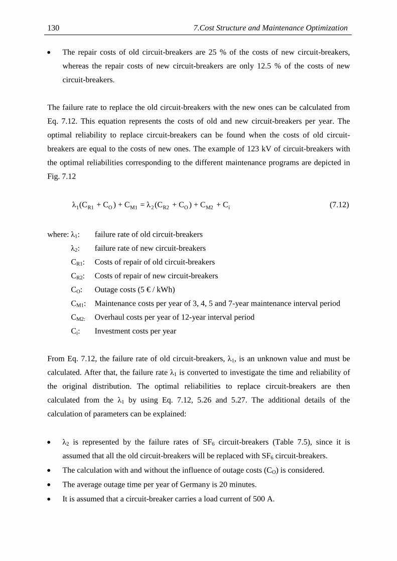
7.Cost Structure and Maintenance Optimization 130
• The repair costs of old circuit-breakers are 25 % of the costs of new circuit-breakers,
whereas the repair costs of new circuit-breakers are only 12.5 % of the costs of new
circuit-breakers.
The failure rate to replace the old circuit-breakers with the new ones can be calculated from
Eq. 7.12. This equation represents the costs of old and new circuit-breakers per year. The
optimal reliability to replace circuit-breakers can be found when the costs of old circuit-
breakers are equal to the costs of new ones. The example of 123 kV of circuit-breakers with
the optimal reliabilities corresponding to the different maintenance programs are depicted in
Fig. 7.12
1 R1 O M1 2 R2 O M2 iλ (C + C ) + C = λ (C + C ) + C + C (7.12)
where: λ1: failure rate of old circuit-breakers
λ2: failure rate of new circuit-breakers
CR1: Costs of repair of old circuit-breakers
CR2: Costs of repair of new circuit-breakers
CO: Outage costs (5 € / kWh)
CM1: Maintenance costs per year of 3, 4, 5 and 7-year maintenance interval period
CM2: Overhaul costs per year of 12-year interval period
Ci: Investment costs per year
From Eq. 7.12, the failure rate of old circuit-breakers, λ1, is an unknown value and must be
calculated. After that, the failure rate λ1 is converted to investigate the time and reliability of
the original distribution. The optimal reliabilities to replace circuit-breakers are then
calculated from the λ1 by using Eq. 7.12, 5.26 and 5.27. The additional details of the
calculation of parameters can be explained:
• λ2 is represented by the failure rates of SF6 circuit-breakers (Table 7.5), since it is
assumed that all the old circuit-breakers will be replaced with SF6 circuit-breakers.
• The calculation with and without the influence of outage costs (CO) is considered.
• The average outage time per year of Germany is 20 minutes.
• It is assumed that a circuit-breaker carries a load current of 500 A.
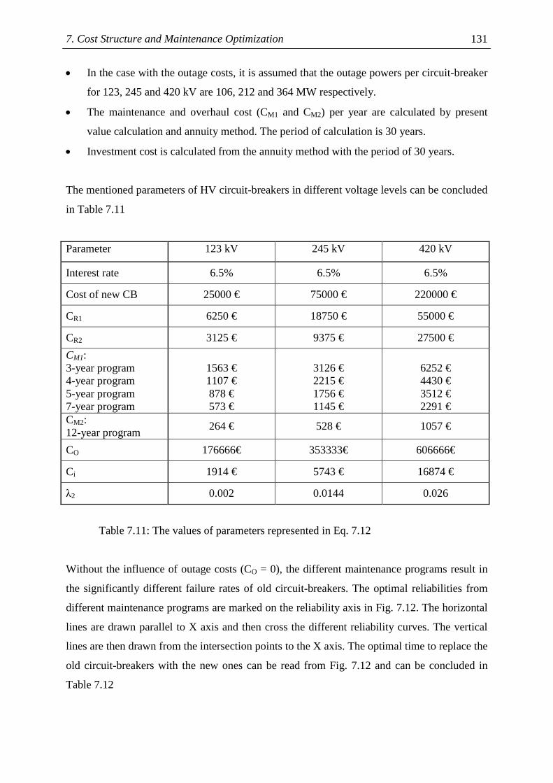
7. Cost Structure and Maintenance Optimization 131
• In the case with the outage costs, it is assumed that the outage powers per circuit-breaker
for 123, 245 and 420 kV are 106, 212 and 364 MW respectively.
• The maintenance and overhaul cost (CM1 and CM2) per year are calculated by present
value calculation and annuity method. The period of calculation is 30 years.
• Investment cost is calculated from the annuity method with the period of 30 years.
The mentioned parameters of HV circuit-breakers in different voltage levels can be concluded
in Table 7.11
Parameter 123 kV 245 kV 420 kV
Interest rate 6.5% 6.5% 6.5%
Cost of new CB 25000 € 75000 € 220000 €
CR1 6250 € 18750 € 55000 €
CR2 3125 € 9375 € 27500 €
CM1: 3-year program 4-year program 5-year program 7-year program
1563 € 1107 € 878 € 573 €
3126 € 2215 € 1756 € 1145 €
6252 € 4430 € 3512 € 2291 €
CM2: 12-year program
264 € 528 € 1057 €
CO 176666€ 353333€ 606666€
Ci 1914 € 5743 € 16874 €
λ2 0.002 0.0144 0.026
Table 7.11: The values of parameters represented in Eq. 7.12
Without the influence of outage costs (CO = 0), the different maintenance programs result in
the significantly different failure rates of old circuit-breakers. The optimal reliabilities from
different maintenance programs are marked on the reliability axis in Fig. 7.12. The horizontal
lines are drawn parallel to X axis and then cross the different reliability curves. The vertical
lines are then drawn from the intersection points to the X axis. The optimal time to replace the
old circuit-breakers with the new ones can be read from Fig. 7.12 and can be concluded in
Table 7.12

7.Cost Structure and Maintenance Optimization 132
Year
Rel
iabi
lity,
Rm(t
)
Figure 7.12: The optimal reliabilities and years to replace the old 123 kV
circuit-breakers
The results from Table 7.12 must be carefully interpreted. It is obvious from the Fig. 7.12 and
Table 7.12 that the 5-year and 7-year maintenance are the optimal maintenance programs
which can prolong the time to replace up to 54 and 39 years while keeping the reliability of
0.66 and 0.58 respectively. Although the 3-year and 4-year maintenance can prolong the times
to replace up to more than 65 years, they cannot be considered as the optimal maintenance,
since the optimal years to replace are beyond the expected lifetime of circuit-breakers.
123 kV Optimal reliability Optimal time to replace (years)
3-year maintenance 0.86 > 65
4-year maintenance 0.73 > 65
5-year maintenance 0.66 54
7-year maintenance 0.58 39
Table 7.12: The optimal years to replace of 123 kV circuit-breakers regarding
the different maintenance programs
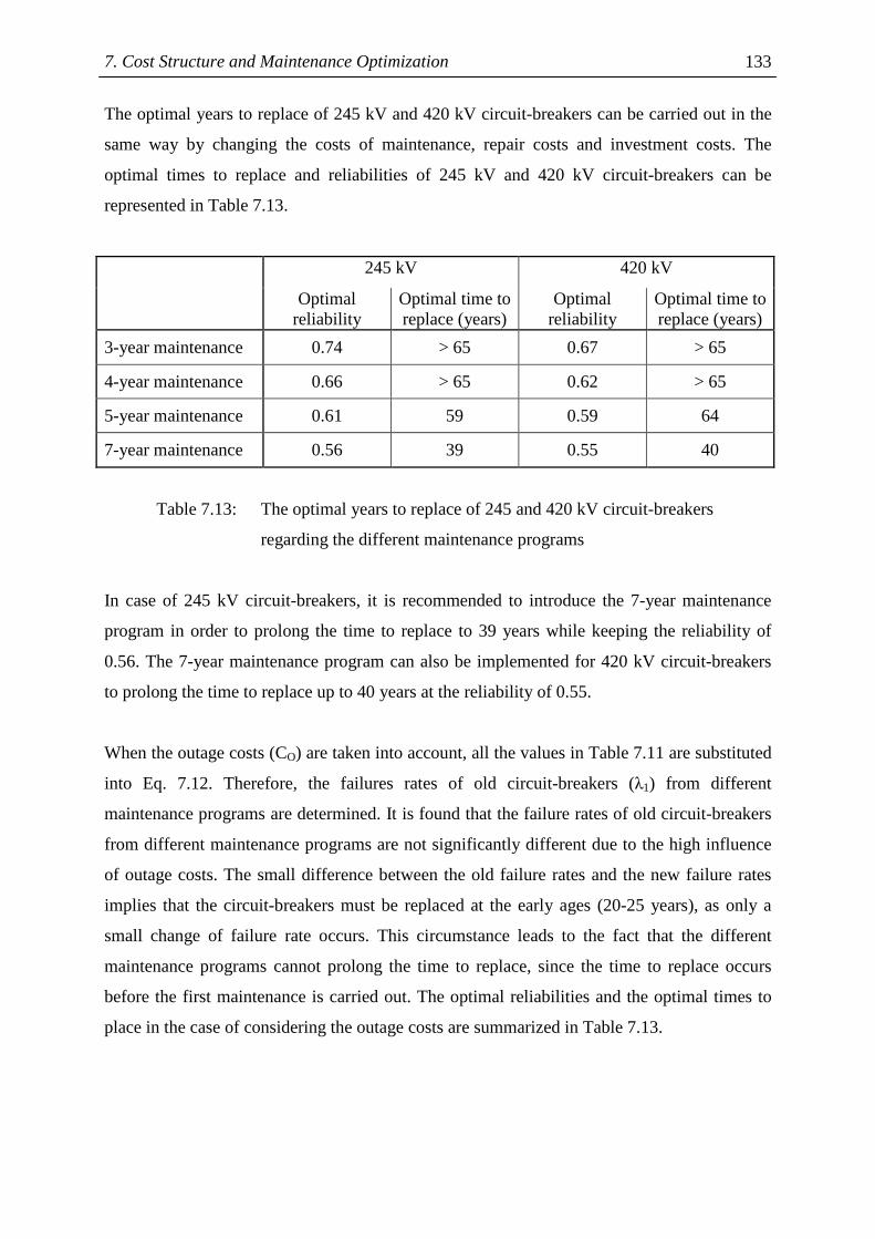
7. Cost Structure and Maintenance Optimization 133
The optimal years to replace of 245 kV and 420 kV circuit-breakers can be carried out in the
same way by changing the costs of maintenance, repair costs and investment costs. The
optimal times to replace and reliabilities of 245 kV and 420 kV circuit-breakers can be
represented in Table 7.13.
245 kV 420 kV
Optimal reliability
Optimal time to replace (years)
Optimal reliability
Optimal time to replace (years)
3-year maintenance 0.74 > 65 0.67 > 65
4-year maintenance 0.66 > 65 0.62 > 65
5-year maintenance 0.61 59 0.59 64
7-year maintenance 0.56 39 0.55 40
Table 7.13: The optimal years to replace of 245 and 420 kV circuit-breakers
regarding the different maintenance programs
In case of 245 kV circuit-breakers, it is recommended to introduce the 7-year maintenance
program in order to prolong the time to replace to 39 years while keeping the reliability of
0.56. The 7-year maintenance program can also be implemented for 420 kV circuit-breakers
to prolong the time to replace up to 40 years at the reliability of 0.55.
When the outage costs (CO) are taken into account, all the values in Table 7.11 are substituted
into Eq. 7.12. Therefore, the failures rates of old circuit-breakers (λ1) from different
maintenance programs are determined. It is found that the failure rates of old circuit-breakers
from different maintenance programs are not significantly different due to the high influence
of outage costs. The small difference between the old failure rates and the new failure rates
implies that the circuit-breakers must be replaced at the early ages (20-25 years), as only a
small change of failure rate occurs. This circumstance leads to the fact that the different
maintenance programs cannot prolong the time to replace, since the time to replace occurs
before the first maintenance is carried out. The optimal reliabilities and the optimal times to
place in the case of considering the outage costs are summarized in Table 7.13.

7.Cost Structure and Maintenance Optimization 134
123 kV 245 kV 420 kV Optimal
reliability Optimal time
to replace (years)
Optimal reliability
Optimal time to replace
(years)
Optimal reliability
Optimal time to replace
(years)
3-year maintenance
0.99 22 0.99 23 0.99 23
4-year maintenance
0.99 22 0.99 23 0.98 24
5-year maintenance
0.99 23 0.99 23 0.98 24
7-year maintenance
0.99 23 0.99 23 0.98 24
Table 7.13: The optimal reliabilities and years to place in the case of taking the
outage costs into consideration
It can be seen from Table 7.13 that the optimal times to replace occur before the first
maintenance programs are performed. In this case, the different preventive maintenance
programs play no important role in order to prolong the times to replace.
Without consideration of outage costs, it is concluded from the optimal maintenance that
different preventive maintenance programs can prolong the lifetimes of circuit-breakers.
However, the life-cycle cost must be taken into consideration in order to find the optimal
times to replace of circuit-breakers. This optimal calculation depends mainly on many
parameters as shown in Eq. 7.12. Consequently, the results of the calculation could be varied
when the parameters are changed.
It is obvious from the life-cycle cost calculation (Eq. 7.12) that the outage costs have the
highest influence. When the high outage costs are taken into account, the difference between
the old failure rates and the new failure rates is significantly small. Consequently, the old
circuit-breakers should be replaced at the early ages (20-25 years). In this situation, the
different maintenance programs have no influence on the time to replace.
8. Conclusions 135
8 Conclusions
The main objectives of this thesis were to analyze the risks of HV circuit-breakers, develop
the probabilistic models, breakdown the cost structure and establish the improved
maintenance strategies. Owing to deregulation of electricity markets, the competitiveness of
markets is significantly concerned. This issue is related with the reliability, availability of
systems and costs of maintenance. HV circuit-breakers which are one of the most important
equipment in power systems have been served as interrupting equipment for operating and
short-circuit currents for more than a century. Many technologies in terms of interrupting
medium had been developed from oil, air-blast, vacuum to SF6. At present, a number of HV
circuit-breakers are reaching the aging period and they are required to be effectively handled.
Some can be prolonged by using the effective maintenance, whereas some must be replaced
before the major failures occur.
Normally, HV circuit-breakers have been maintained by using manufacturers’ guidelines and
experiences of operators. It is not well proved that such maintenance programs are effective
regarding costs and performance. Although there are many literatures introducing the optimal
maintenance for HV circuit-breakers, most of them propose only the ideas and mathematical
models without the reference from the failure database. In this context it was challenging to
design and investigate reliability and maintenance strategies in connection with the failure
database.
This thesis was constructed of three main parts to handle such problems. In the first part, the
failure modes and effects analysis method was applied to determine the risks of components
of HV circuit-breakers. The second part was to develop the probabilistic models to investigate
the reliability of HV circuit-breakers and failure development. In the last part the cost
structure of HV circuit-breakers was determined. In addition, the optimal maintenance
strategies during useful and wear-out period were established. The failure database of HV
circuit-breakers collected by the Institute of Power Systems, Darmstadt University of
Technology had been implemented in all parts.
In order to conduct the failure modes and effects analysis method, the functions of HV circuit-
breakers and their functional failure modes were first defined. Next, the causes of failure

8. Conclusions 136
related to the function and components were investigated and the numbers of failures were
taken from the database. The consequences of each failure including personnel safety,
environmental impact, operation availability and costs of repair were evaluated by using a
score system. The criteria of failure detection must be considered to evaluate the severity of
failures. Consequently, the risks of HV circuit-breaker components composed of the
consequence of failure, the failure detection and the probability of failure could be calculated
and the ranking of risk is then represented. The weighing factors for such three parameters
were determined by using the decision matrix approach. It was discovered from the risk
diagram that the components of HV circuit-breakers are in the low and medium risk region.
The improved maintenance strategies should be applied to the components which are in the
medium risk region to assure that those components will not reach the high risk region. The
disadvantage of the risk diagram is that it is a time-independent diagram. Consequently, the
diagram cannot predict which component should be replaced at which year.
The probabilistic models were developed to investigate the reliability of HV circuit-breakers
and how the failures develop from year to year. The first model, treeing diagram, is the model
representing the probability of failures occurring in any subsequent years. The development
of failures from the failure-free state to the first and second failures was investigated by using
the conditional probability method and represented as a treeing diagram. The critical
pathways of failure development could be investigated with this model. The second model,
the cascading reliability model, was the extension of the treeing diagram. The development of
failures from failure-free state to the first, second and third failures was represented in terms
of mean time to failure, transition and state probabilities. With this model, it is possible to
discover when the failures could occur and at which probability. It is beneficial for the asset
managers and maintenance personnel to be aware of the following failures. The last
probabilistic model is the reliability model obtained by using the application of Markov
process. In this model, HV circuit-breakers are composed of five main components. The
reliability parameters such as mean time to failure and mean time to repair of each component
were examined from the database. By using the Markov process method, the failure-free
durations and availability of different types of HV circuit-breakers can be investigated. It was
concluded from this Markov model that the availability of HV circuit-breakers is over 99%.
The influence of repetitive failures resulting from human error or incomplete repair was taken
into consideration.
8. Conclusions 137
In the first part of the last section, the cost structure of HV circuit-breakers related to
specifications was broken down by using the decision matrix approach. This decision matrix
was also applied to each main component resulting in the detailed cost structure. It was found
from the cost breakdown that “rated voltage” has the highest influence on the total costs
followed by “rated short circuit breaking current” and “rated lighting and switching impulse
withstand voltage”. The cost structure provides the valuable information for the designers to
design the cost-effective HV circuit-breakers for different applications.
Maintenance optimization was the last issue in this thesis. It can be divided into two periods:
useful life and wear-out period. These periods were handled with the different maintenance
models. The optimal maintenance frequency during useful life period was established from
the principle that more frequent maintenance could result in more system downtime; on the
other hand, less maintenance could result in downtime due to failures. The mathematical
model and the failure rates of HV circuit-breakers were applied. The different types of HV
circuit-breakers at different voltage levels were taken into consideration. It was found that the
minor and major maintenance for 123 kV HV circuit-breakers should be performed every 8-
10 and 24-33 years respectively. For 245 kV, the 4-year interval minor and 14-year interval
major maintenance are suggested to be implemented. For the voltage level of 420 kV, it is
suggested to introduce the minor and major maintenance every 3-4 and 8-10 years
respectively.
During the wear-out period, the failure rate of HV circuit-breakers represents the Weibull
distribution. With the preventive maintenance, it is possible to increase the reliability during
this period. Nevertheless, the more frequent maintenance results in the more costs of
maintenance. Therefore, the optimal maintenance was considered by taking the costs of
repair, costs of undelivered energy, costs of maintenance and costs of investment into
account. The different preventive maintenance programs show the different results regarding
the reliability of HV circuit-breakers and optimal time to replace the old circuit-breakers with
the new ones. It must be noted that this optimal maintenance model considerably relates to
mentioned costs. The results could be changed when one or more costs are changed.
The optimal maintenance programs during useful life and wear-out period are very useful for
asset managers to make a decision when and what kind of maintenance should be performed.
8. Conclusions 138
It is recommended that this optimal maintenance could be investigated in more detail in terms
of the sensitivity of the different cost parameters.

Bibliography 139
Bibliography
[1] G. Mazza and R. Michaca, “The first international enquiry on high voltage circuit-
breaker failures and defects in services,” Electra no.79, pp. 21-91, Dec. 1981.
[2] CIGRE Technical Brochure, “Final report of the 2nd international enquiry on HV
circuit-breaker failures and defects in service,” No.83, 1994.
[3] A.L.J. Janssen, “CIGRE WG 13.06 studies on the reliability of single pressure SF6-gas
high voltage circuit-breakers,” IEEE Trans. on Power Delivery, Vol. 11, No. 1, pp. 274-
282, Jan. 1996.
[4] C. Neumann, G. Balzer, J. Becker, R. Meister, V. Rees and C.E. Sölver, “Stress of HV
circuit-breakers during operation in the networks-German utilities’ experience,” CIGRE
SC13, report 13-304, 2002.
[5] Wechselstromschaltgeräte für Spannungen über 1 kV: Hochspannungs-Wechselstrom-
Leistungsschalter, Allgemeines und Begriffe, DIN VDE 0670-101/12.92.
[6] IEEE Standard Rating Structure for AC High-Voltage Circuit Breakers Rated on a
Symmetrical Current Basis, IEEE Standard C37.04-1979, 1979.
[7] IEC Standard High Voltage Switchgear and Controlgear, IEC 62271-100, 2001.
[8] CIGRE Working Group 13.09, “User guide for the application of monitoring and
diagnostic techniques for switching equipment for rated voltages of 72.5 kV and above,
Aug. 2000.
[9] L. van der Sluis, Transients in Power Systems, England: John Wiley & Sons, 2001.
[10] R.D. Garzon, High Voltage Circuit Breakers: Design and Applications, New York;
Marcel Dekker, 2002.
Bibliography 140
[11] R.Radwan, “Circuit breaking,” in High-Voltage Engineering: Theory and Practice, 2nd
ed., M. Abdel-Salam, Ed. New York: Marcel Dekker Inc., 2001, pp. 335-372.
[12] C. Neumann, “Hochspannungsschaltgeräte und anlagen,” Script zur Vorlesung, April,
2002.
[13] S.M. Ghufran Ali, “Switching design, development and service,” in High Voltage
Engineering and Testing, 2nd ed., H.M. Ryan, Ed. London: The Institution of Electrical
Engineering, 2001, pp. 301-334.
[14] A. Greenwood, Electrical Transients in Power Systems, 2nd ed., New York: John Wiley
& Sons, 1991.
[15] A.B. Johnson, A. J. Schultz, N. R. Schultz and R. B. Shores, “Some Fundamentals on
Capacitance Switching,” Transactions of the AIEE, Vol. 74, Part III, pp. 727-736, Aug.
1955.
[16] CIGRE Working Group 13.04, “Shunt Capacitor Bank Switching: Stresses and Test
Methods (First Part),” ELECTRA, No. 182, pp. 165-189, Feb. 1999.
[17] G. Balzer, “Energieversorgung: Teil 1,” Script zur Vorlesung, 2006.
[18] I. Uglesic, S. Hutter, M. Krepela, B.F. Grcic and F. Jakl, “Transients due to switching of
400 kV shunt reactor,” in Proc. International Conference on Power Systems Transients,
2001.
[19] M. Popov and E. Acha, “Overvoltages due to switching off an unloaded transformer
with a vacuum circuit breaker,” IEEE Trans. Power Delivery, Vol. 14, No. 4, pp. 1317-
1326, Oct. 1999.
[20] IEEE Standard for AC High-Voltage Generator Circuit Breakers Rated on a
Symmetrical Current Basis, IEEE Standard C37.013-1997, 1997.

Bibliography 141
[21] D. Dufournet and J.M. Willieme, “Generator circuit breakers: SF6 breaking chamber –
Interruption of current with non-zero passage – Influence of cable connection on TRV
of system fed faults,” in Proc. CIGRE Session 2002, 13-101.
[22] A.L.J. Janssen, W. Degen, C.R. Heising, H. Bruvik, E. Colombo, W.Lanz, P.Fletcher
and G. Sanchis, “A summary of the final results and conclusions of the second
international enquiry on the reliability of high voltage circuit breakers,” CIGRE 13-202,
1994 Session.
[23] C.R. Heising, “Worldwide reliability survey of high-voltage circuit breakers,” IEEE
Industry Applications Magazine, pp. 65-66, May/June 1996.
[24] J. Becker, “Schaltbeanspruchungen von Hochspannungs-Leistungsschaltern im
Netzbetrieb,” Ph.D.dissertation, Dept. Elec Eng., TU-Darmstadt, 2001.
[25] IEC Standard Common Specifications for High-Voltage Switchgear and Control
Standards, IEC 60694, 2001.
[26] C. Neumann, G. Balzer, J. Becker, R. Meister, V. Rees and C.E. Sölver, “Stress of HV
Circuit-Breakers during Operation in the Networks-German Utilities’ Experience,”
CIGRE SC13, report 13-304, 2002.
[27] J. Becker, G. Balzer, R. Meister and C. Neumann, “Beanspruchungen von
Hochspannungs-Leistungsschaltern an Beispiel zweier EVU,” Elektrizitätswirtschaft,
Jg. 99, Heft 11, 2000.
[28] G. Catenacci, L. Paris, J.P. Couvreux and M. Pouard, “Transient recovery voltages in
French and Italian high-voltages networks,” IEEE, PAS 1986(11), pp. 1420-1431, 1967.
[29] A. Braun, K.H. Hinterthür, H. Lipken, B. Stein and O. Völker, “Characteristic values of
the transient recovery voltage for different types of short circuits in an extensive 420kV
system,” ETZ-A, no. 97, pp. 489-493, 1976.

Bibliography 142
[30] CIGRE Working Group 33.02, “Guidelines for Representation of Network Elements
When Calculating Transients,” 1990.
[31] A.L.J. Janssen and C.E. Sölver, “ The statistics behind the electrical endurance type test
for HV circuit-breakers applied by CIGRE SC A3/WG13.08 and IEC SC 17A/WG29,”
CIGRE, report A3-304, 2004.
[32] F.S. Nowlan and H.F. Heap, “Reliability-Centered Maintenance,” National Technical
Information Service, U.S. Department of Commerce., Springfield, Virginia, U.S., 1978.
[33] A.M. Smith, “Reliability-Centered Maintenance,” McGraw-Hill, U.S., 1993.
[34] J. Moubray, “Reliability-centered Maintenance,” New York, Industrial Press Inc., 1997.
[35] M. Rausand and J. Vatn, “Reliabiliy Centered Maintenance. In C. G. Soares, editor,
Risk and Reliability in Marine Technology,” Balkema, Holland, 1998.
[36] G. Balzer, O. Schmitt, A. Schneider, S. Gal, F. Balasiu and K. Bakic, “Life cycle
assessment of substations: a procedure for an optimized asset management,” in Proc.
CIGRE Session 2002, 23-302.
[37] G. Balzer, E. Bakic and H.J. Haubrich, C. Neumann and C. Schorn, “Selection of an
optimal maintenance and replacement strategy of H.V. equipment by a risk assessment
process,” in Proc. CIGRE 2006, B3-103.
[38] T. Chan, C.C. Liu and J.W. Choe, “Implementation of reliability-centered maintenance
for circuit breakers,” in Proc. IEEE/PES General Meeting, Vol. 1, pp. 684-690. 2005.
[39] L. Bertling, R. Allan and R. Eriksson, “A reliability-centered asset maintenance method
for assessing the impact of maintenance in power distribution systems,” IEEE Trans.
Power Systems, Vol. 20, No. 1, pp. 75-82, Feb. 2005.
[40] D. Drescher, “Rechnergestützte Bewertung von Betriebsmitteln für
Instandhaltungsstrategien,” Ph.D.dissertation, Dept. Elec Eng., TU-Darmstadt, 2004.

Bibliography 143
[41] IEEE Guide for the Selection of Monitoring for Circuit Breakers, IEEE Standard
C37.10.1-2000, 2000.
[42] J. Gausemaier, A. Fink and O. Schalke, “Szenario-Management,” 2nd ed., München:
Carl Hanser, 1996, p. 189.
[43] R. Billinton and R.N. Allan, Reliability Evaluation of Engineering Systems: Concepts
and Techniques, 2nd ed., New York: Springer, 2005.
[44] C. E. Eberling, An Introduction to Reliability and Maintainability Engineering, New
York: McGraw-Hill, 1997.
[45] R. Billinton and R.N. Allan, Reliability Evaluation of Power Systems, 2nd ed., New
York: Springer, 2001.
[46] S. Natti, P. Jirutitijaroen, M. Kezunovic, and C. Singh, “Circuit breaker and transformer
inspection and maintenance: probabilistic models,” in Proc. 8th international conference
on probabilistic methods applied to power systems, 2004, pp.1003-1008.
[47] T. Lindquist, L. Bertling, and R. Eriksson, “A feasibility study for probabilistic
modeling of aging in circuit breakers for maintenance optimization,” in Proc. 8th
international conference on probabilistic methods applied to power systems, 2004,
pp.1020-1025.
[48] J. Endrenyi, G. J. Anders, and A. M. Leite da Silva, “Probabilistic evaluation of the
effect of maintenance on reliability – an application,” IEEE Trans. Power Systems, Vol.
13, No. 2, pp. 576-583, May 1998.
[49] D. Drescher, G. Balzer, and C. Neumann, “Preparing failure data to evaluate electrical
equipment and results,” in Proc. 13th international symposium on high voltage
engineering, 2003.

Bibliography 144
[50] D. Drescher, and G. Balzer, “A new method for qualitative and quantitative evaluation
of ageing behaviour of electrical equipment,” in Proc. 13th international symposium on
high voltage engineering, 2003.
[51] J. Endrenyi, Reliability Modeling in Electric Power Systems, Wiley, 1978, p.52.
[52] A. K. S. Jardine, and A. H. C. Tsang, Maintenance, Replacement, and Reliability:
Theory and Application, CRC Press, 2006.
Contributions by the Author
[1] P. Choonhapran and G. Balzer, “Study of Stresses of Circuit-Breakers:
CombinedStatistical Method,” in Proc. 9th IEEE International Conference on
Probabilistic Methods Applied to Power Systems, Kungliga Tekniska Högskolan,
Stockholm, Sweden, June 11-15, 2006.
[2] P. Choonhapran, G. Balzer and B.Rusek, “FMEA-Methode als Hilfsmittel für eine
diagnose von Hochspannungs-Leistungsschaltern,” in Proc. of the Diagnostik 2006,
Kassel, Germany, 19-20 September, 2006.
[3] P. Choonhapran and G.Balzer, “Stresses of Circuit-Breakers: Effects of Grounding and
Types of Applications,” in Proc. of the 2006 IEEE PES Power Systems Conference and
Exposition, Atlanta, Georgia, October 2006.
[4] P. Choonhapran and G. Balzer, “Availability of HV Circuit-Breakers: The Application
of Markov Model,” in Proc. of the 2007 PES General Meeting, Tampa, Florida, June
2007.
[5] P.Choonhapran and G. Balzer, “Cascading Reliability Model for HV Circuit-Breakers,”
in Proc. of the Power Tech 2007, Lausanne, Switzerland, July, 2007.

List of Symbols and Abbreviations 145
List of Symbols and Abbreviations
Symbols
Al2O3 Aluminium oxide
CaO Calcium oxide
f(t) Probability density function
Ik1TF Single-phase short circuit-current at terminal
Ik3TF Three-phase short circuit-current at terminal
Iload Load current
Ir Rated normal current
Irb Rated short-circuit breaking current
Isc Short-circuit current
MTTF Mean time to failure
MTTR Mean time to repair
NaOH Sodium hydroxide
N2 Nitrogen
fN (t) Number of component failed at time t
sN (t) Number of components surviving at time t
Q(t) Cumulative distribution function
R(t) Survivor function
SF6 Sulphur hexafluoride
Zw Characteristic impedance
λ(t) Failure rate
2δ Variance
β Shape parameter of Weibull distribution
α Scale parameter of Weibull distribution
ω Operating frequency

List of Symbols and Abbreviations 146
Abbreviations
EPRI Electric Power Research Institute
FMEA Failure Modes and Effects Analysis
HV High Voltage
IEEE Institute of Electrical and Electronics Engineers
RCM Reliability-Centred Maintenance
RRRV Rate of Rise of Recovery Voltage
TRV Transient Recovery Voltage
XLPE Cross-linked polyethylene
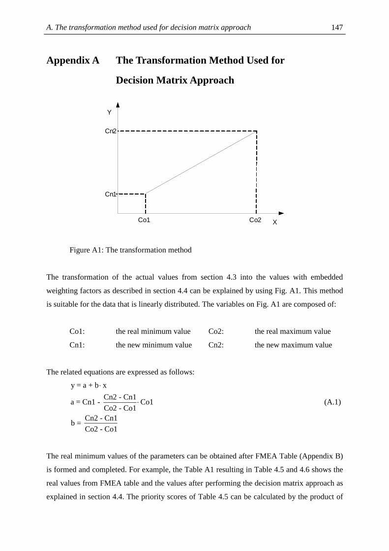
A. The transformation method used for decision matrix approach 147
Appendix A The Transformation Method Used for
Decision Matrix Approach
Y
XCo1 Co2
Cn1
Cn2
Figure A1: The transformation method
The transformation of the actual values from section 4.3 into the values with embedded
weighting factors as described in section 4.4 can be explained by using Fig. A1. This method
is suitable for the data that is linearly distributed. The variables on Fig. A1 are composed of:
Co1: the real minimum value Co2: the real maximum value
Cn1: the new minimum value Cn2: the new maximum value
The related equations are expressed as follows:
y = a + b x
Cn2 - Cn1a = Cn1 - Co1
Co2 - Co1Cn2 - Cn1
b = Co2 - Co1
⋅
⋅ (A.1)
The real minimum values of the parameters can be obtained after FMEA Table (Appendix B)
is formed and completed. For example, the Table A1 resulting in Table 4.5 and 4.6 shows the
real values from FMEA table and the values after performing the decision matrix approach as
explained in section 4.4. The priority scores of Table 4.5 can be calculated by the product of

A. The Transformation Method Used for Decision Matrix Approach 148
transformation of parameters 1,2 and 3, while the scores of Table 4.6 are calculated from
parameter 1,2 and 4.
Real values Transformed values Parameter
minimum maximum minimum maximum
1.Consequence of failure 1 28 1 17
2.Failure detection 1 3 1 50
3.Probability of failure by functional failure
7.7e-05 0.055 1 33
4.Probability of failure by component
7.0e-04 0.073 1 33
Table A1: The real values and transformed values.
By using the equation A.1, the transformed equation can be obtained as stated:
1. Consequence of failure: y = 0.4074 + 0.5926x (A.2)
2. Failure detection y = -23.5 + 24.5x (A.3)
3. Probability of failure by functional failure y = 0.996 + 0.1363x (A.4)
4. Probability of failure by component y = 0.69 + 0.103x (A.5)
The parameters for calculating the total consequences of section 4.6, risk diagram, are
composed of only the consequence of failure and the failure detection. The decision matrix
between these 2 parameters had been applied. It is found that the weighting ration between the
failure detection and the consequence of failure is 75:25. By using the equation A.1, the
transformed equations can be obtained.
1. Consequence of failure y = 0.111 + 0.888x (A.6)
2. Failure detection y = -36 + 37x (A.7)
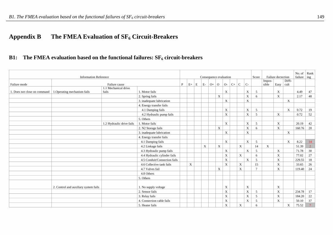
B1. The FMEA evaluation based on the functional failures of SF6 circuit-breakers
149
Appendix B The FMEA Evaluation of SF6 Circuit-Breakers
B1: The FMEA evaluation based on the functional failures: SF6 circuit-breakers
Information Reference Consequence evaluation Score Failure dectection No. of failure
Ranking
Failure mode Failure cause P E+ E E- O+ O O- C+ C C- Impos- sible Easy
Diffi-cult
1. Does not close on command 1.Operating mechanism fails 1.1 Mechanical drive fails 1. Motor fails X X 5 X 4.49 47
2. Spring fails X X 6 X 2.17 48
3. inadequate lubrication X X X
4. Energy transfer fails
4.1 Damping fails X X 5 X 0.72 19
4.2 Hydraulic pump fails X X 5 X 0.72 52
5. Others
1.2 Hydraulic drive fails 1. Motor fails X X 5 X 20.19 42
2. N2 Storage fails X X 6 X 160.76 20
3. inadequate lubrication X X X
4. Energy transfer fails
4.1 Damping fails X X 5 X 8.22 14
4.2 Linkage fails X X X 14 X 51.39 2
4.3 Hydraulic pump fails X X 5 X 71.78 30
4.4 Hydraulic cylinder fails X X 6 X 77.02 27
4.5 Conduit/Connection fails X X 5 X 229.55 18
4.6 Collective tank fails X X X 15 X 33.65 26
4.7 Valves fail X X 7 X 119.40 24
4.8 Others
5. Others
2. Control and auxiliary system fails 1. No supply voltage X X X
2. Sensor fails X X 5 X 234.78 17
3. Relay fails X X 5 X 184.20 22
4. Connection cable fails X X 5 X 50.10 37
5. Heater fails X X 6 X 75.52 7
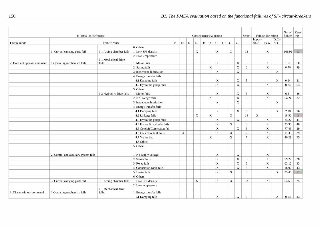
B1. The FMEA evaluation based on the functional failures of SF6 circuit-breakers
150
Information Reference
Consequence evaluation Score Failure dectection No. of failure
Ranking
Failure mode Failure cause P E+ E E- O+ O O- C+ C C-
Impos- sible Easy
Diffi-cult
6. Others
3. Current carrying parts fail 3.1 Arcing chamber fails 1. Low SF6 density X X X 13 X 161.92 13
2. Low temperature
2. Does not open on command 1.Operating mechanism fails 1.1 Mechanical drive fails 1. Motor fails X X 5 X 1.51 50
2. Spring fails X X 6 X 0.76 49
3. inadequate lubrication X X X
4. Energy transfer fails
4.1 Damping fails X X 5 X 0.24 21
4.2 Hydraulic pump fails X X 5 X 0.24 54
5. Others
1.2 Hydraulic drive fails 1. Motor fails X X 5 X 6.81 46
2. N2 Storage fails X X 6 X 54.24 32
3. inadequate lubrication X X X
4. Energy transfer fails
4.1 Damping fails X X 5 X 2.78 16
4.2 Linkage fails X X X 14 X 18.50 3
4.3 Hydraulic pump fails X X 5 X 24.22 41
4.4 Hydraulic cylinder fails X X 6 X 25.98 40
4.5 Conduit/Connection fail X X 5 X 77.45 29
4.6 Collective tank fails X X X 15 X 11.35 39
4.7 Valves fail X X 7 X 40.29 35
4.8 Others
5. Others
2. Control and auxiliary system fails 1. No supply voltage X X X
2. Sensor fails X X 5 X 79.22 28
3. Relay fails X X 5 X 62.15 33
4. Connection cable fails X X 5 X 16.90 43
5. Heater fails X X 6 X 25.48 12
6. Others
3. Current carrying parts fail 3.1 Arcing chamber fails 1. Low SF6 density X X X 13 X 54.63 25
2. Low temperature
3. Closes without command 1.Operating mechanism fails 1.1 Mechanical drive fails 1. Energy transfer fails
1.1 Damping fails X X 5 X 0.03 23
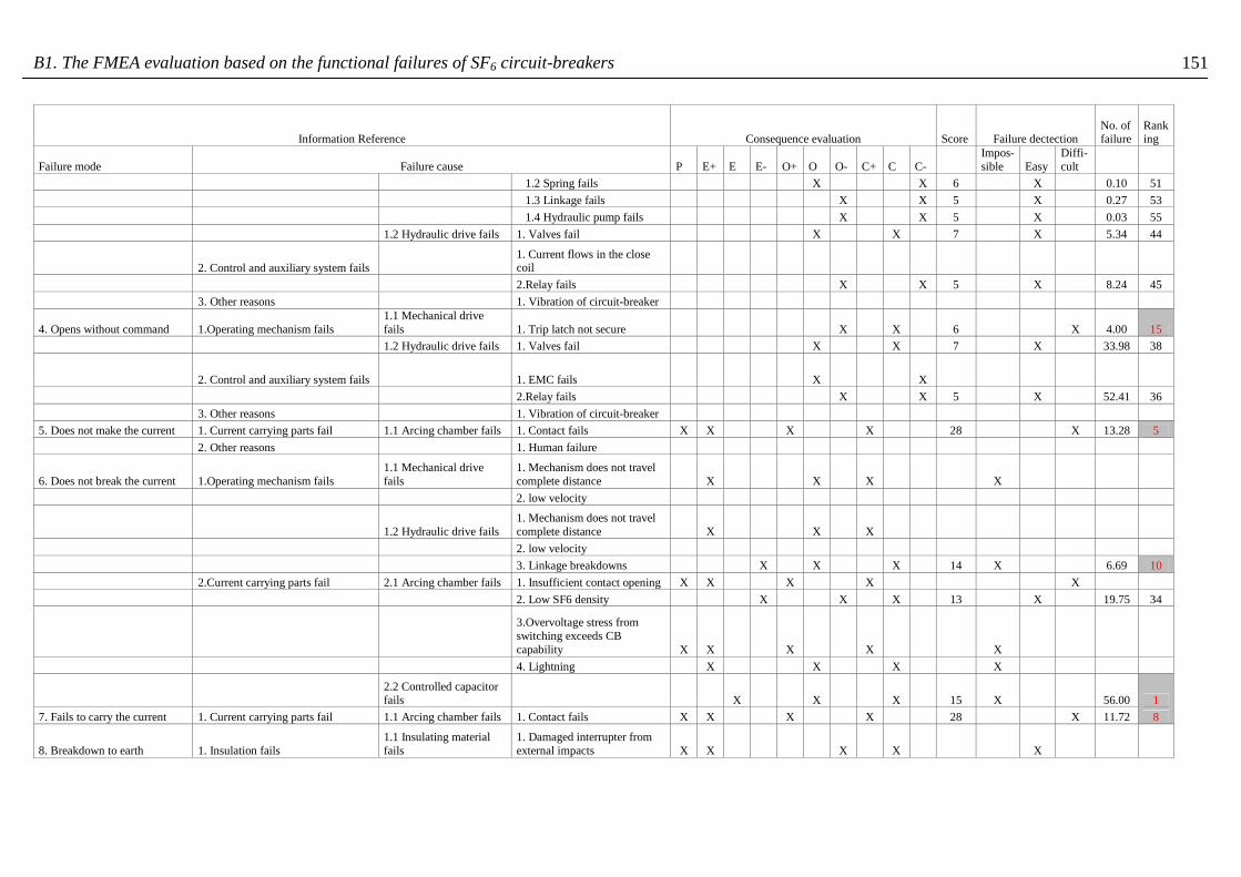
B1. The FMEA evaluation based on the functional failures of SF6 circuit-breakers
151
Information Reference
Consequence evaluation Score Failure dectection No. of failure
Ranking
Failure mode Failure cause P E+ E E- O+ O O- C+ C C-
Impos- sible Easy
Diffi-cult
1.2 Spring fails X X 6 X 0.10 51
1.3 Linkage fails X X 5 X 0.27 53
1.4 Hydraulic pump fails X X 5 X 0.03 55
1.2 Hydraulic drive fails 1. Valves fail X X 7 X 5.34 44
2. Control and auxiliary system fails 1. Current flows in the close coil
2.Relay fails X X 5 X 8.24 45
3. Other reasons 1. Vibration of circuit-breaker
4. Opens without command 1.Operating mechanism fails 1.1 Mechanical drive fails 1. Trip latch not secure X X 6 X 4.00 15
1.2 Hydraulic drive fails 1. Valves fail X X 7 X 33.98 38
2. Control and auxiliary system fails 1. EMC fails X X
2.Relay fails X X 5 X 52.41 36
3. Other reasons 1. Vibration of circuit-breaker
5. Does not make the current 1. Current carrying parts fail 1.1 Arcing chamber fails 1. Contact fails X X X X 28 X 13.28 5
2. Other reasons 1. Human failure
6. Does not break the current 1.Operating mechanism fails 1.1 Mechanical drive fails
1. Mechanism does not travel complete distance X X X X
2. low velocity
1.2 Hydraulic drive fails 1. Mechanism does not travel complete distance X X X
2. low velocity
3. Linkage breakdowns X X X 14 X 6.69 10
2.Current carrying parts fail 2.1 Arcing chamber fails 1. Insufficient contact opening X X X X X
2. Low SF6 density X X X 13 X 19.75 34
3.Overvoltage stress from switching exceeds CB capability X X X X X
4. Lightning X X X X
2.2 Controlled capacitor fails X X X 15 X 56.00 1
7. Fails to carry the current 1. Current carrying parts fail 1.1 Arcing chamber fails 1. Contact fails X X X X 28 X 11.72 8
8. Breakdown to earth 1. Insulation fails 1.1 Insulating material fails
1. Damaged interrupter from external impacts X X X X X
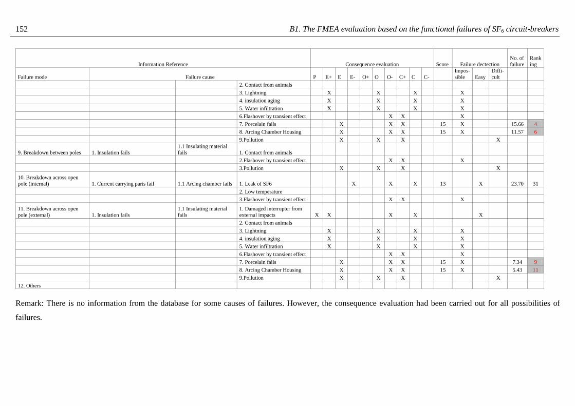
B1. The FMEA evaluation based on the functional failures of SF6 circuit-breakers
152
Information Reference
Consequence evaluation Score Failure dectection No. of failure
Ranking
Failure mode Failure cause P E+ E E- O+ O O- C+ C C-
Impos- sible Easy
Diffi-cult
2. Contact from animals
3. Lightning X X X X
4. insulation aging X X X X
5. Water infiltration X X X X
6.Flashover by transient effect X X X
7. Porcelain fails X X X 15 X 15.66 4
8. Arcing Chamber Housing X X X 15 X 11.57 6
9.Pollution X X X X
9. Breakdown between poles 1. Insulation fails 1.1 Insulating material fails 1. Contact from animals
2.Flashover by transient effect X X X
3.Pollution X X X X
10. Breakdown across open pole (internal) 1. Current carrying parts fail 1.1 Arcing chamber fails 1. Leak of SF6 X X X 13 X 23.70 31
2. Low temperature
3.Flashover by transient effect X X X
11. Breakdown across open pole (external) 1. Insulation fails
1.1 Insulating material fails
1. Damaged interrupter from external impacts X X X X X
2. Contact from animals
3. Lightning X X X X
4. insulation aging X X X X
5. Water infiltration X X X X
6.Flashover by transient effect X X X
7. Porcelain fails X X X 15 X 7.34 9
8. Arcing Chamber Housing X X X 15 X 5.43 11
9.Pollution X X X X
12. Others
Remark: There is no information from the database for some causes of failures. However, the consequence evaluation had been carried out for all possibilities of
failures.

B2. The FMEA evaluation based on component failures of SF6 circuit-breakers
153
B2: The FMEA evaluation based on component failures: SF6 circuit-breakers
Consequence evaluation Failure detection No. of failure
Conse- quence
Fault detec-tion Ranking
failure cause
failure characteristic
P
E+
E
E-
O+
O
O-
C+
C
C- Impos- sible
Easy
Diffi cult
1.Operating mechanism fails 1.1 Mechanical drive fails 1. Motor fails X X X 6 5 1 20 2. Spring fails X X X 3 6 1 21 3. inadequate lubrication X X X 4. Energy transfer fails 4.3 Trip latch not secure (closing latch) X X X 6 6 2 9 5. Mechanism does not travel complete distance X X X X 1.2 Hydraulic drive fails 1. Motor fails X X X 27 5 1 19 2. N2 Storage fails X X X 215 6 1 14 3. inadequate lubrication X X X 4. Energy transfer fails 4.1 Damping fails X X X 12 5 2 8 4.2 Linkage fails X X X X 75 14 3 1 4.3 Hydraulic pump fails X X X 96 5 1 17 4.4 Hydraulic cylinder fails X X X 103 6 1 16 4.5 Conduit/Connection fails X X X 307 5 1 11 4.6 Collective tank fails X X X X 45 15 1 15 4.7 Valves fail X X X 199 7 1 13 5. Mechanism does not travel complete distance X X X X 2. Control and au1iliary system fails 1. No supply voltage X X X 2. Sensor fails X X X 314 5 1 10 3. Relay fails X X X 307 5 1 11 4. Connection cable fails X X X 67 5 1 18 5. Heater fails X X X 101 6 2 6 6. EMC fails X X X 6 3 3. Current carrying parts fail 3.1 Arcing chamber fails 1. Low SF6 density X X X X 260 13 1 7 2. Contact fails X X X X X 25 28 2 4 3. Insufficient contact opening X X X X X 4.Overvoltage stress from switching
exceeds CB capability X X X X X

B2. The FMEA evaluation based on component failures of SF6 circuit-breakers
154
Consequence evaluation Failure detection No. of failure
Conse- quence
Fault detec-tion Ranking
failure cause
failure characteristic
P
E+
E
E-
O+
O
O-
C+
C
C- Impos- sible
Easy
Diffi cult
3.2 Controlled capacitor fails
X X X X
56 15 3 2 4. Insulation fails 4.1 Insulating material fails 1. Damaged interrupter from external impacts X X X X X 2. Lightning X X X X 3. insulation aging X X X X 4. Water infiltration X X X X 5.Flashover by transient effect X X X 6. Porcelain fails X X X X 23 15 3 3 7. Arcing Chamber fails X X X X 17 15 3 5 8. Pollution X X X X
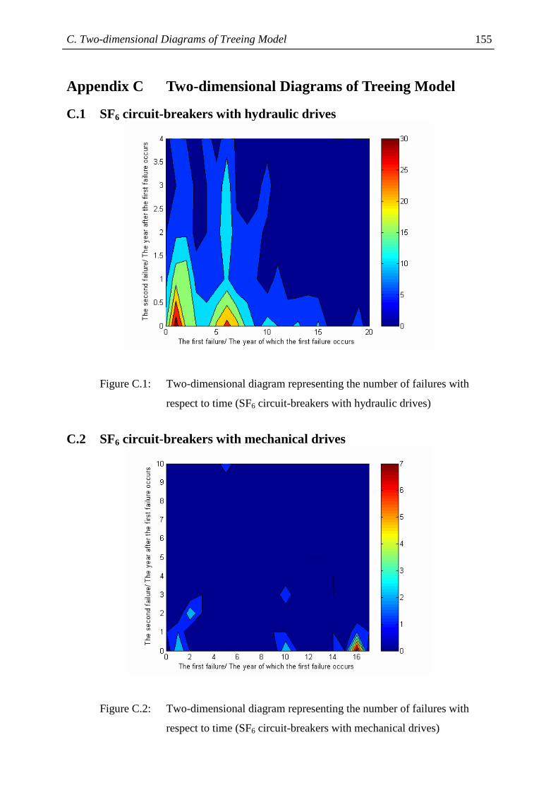
C. Two-dimensional Diagrams of Treeing Model
155
Appendix C Two-dimensional Diagrams of Treeing Model
C.1 SF6 circuit-breakers with hydraulic drives
Figure C.1: Two-dimensional diagram representing the number of failures with
respect to time (SF6 circuit-breakers with hydraulic drives)
C.2 SF6 circuit-breakers with mechanical drives
Figure C.2: Two-dimensional diagram representing the number of failures with
respect to time (SF6 circuit-breakers with mechanical drives)

C. Two-dimensional Diagrams of Treeing Model
156
C.3 Oil circuit-breakers with hydraulic drives
Figure C.3: Two-dimensional diagram representing the number of failures with
respect to time (oil circuit-breakers with hydraulic drives)
C.4 Oil circuit-breakers with mechanical drives
Figure C.4: Two-dimensional diagram representing the number of failures with
respect to time (oil circuit-breakers with mechanical drives)
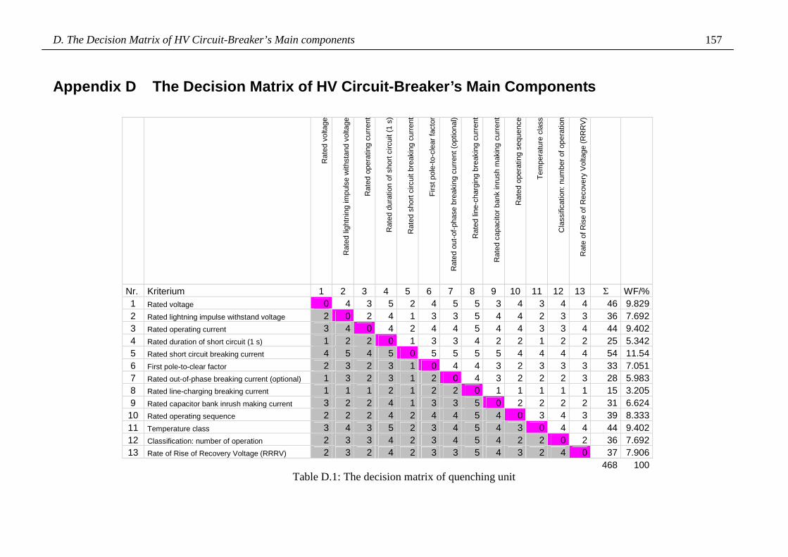
D. The Decision Matrix of HV Circuit-Breaker’s Main components 157
Appendix D The Decision Matrix of HV Circuit-Breake r’s Main Components
Rat
ed v
olta
ge
Rat
ed li
ghtn
ing
impu
lse
with
stan
d vo
ltage
Rat
ed o
pera
ting
curr
ent
Rat
ed d
urat
ion
of s
hort
circ
uit (
1 s)
Rat
ed s
hort
circ
uit b
reak
ing
curr
ent
Firs
t pol
e-to
-cle
ar fa
ctor
Rat
ed o
ut-o
f-ph
ase
brea
king
cur
rent
(op
tiona
l)
Rat
ed li
ne-c
harg
ing
brea
king
cur
rent
Rat
ed c
apac
itor
bank
inru
sh m
akin
g cu
rren
t
Rat
ed o
pera
ting
sequ
ence
Tem
pera
ture
cla
ss
Cla
ssifi
catio
n: n
umbe
r of
ope
ratio
n
Rat
e of
Ris
e of
Rec
over
y V
olta
ge (
RR
RV
)
Nr. Kriterium 1 2 3 4 5 6 7 8 9 10 11 12 13 Σ WF/% 1 Rated voltage 0 4 3 5 2 4 5 5 3 4 3 4 4 46 9.829 2 Rated lightning impulse withstand voltage 2 0 2 4 1 3 3 5 4 4 2 3 3 36 7.692 3 Rated operating current 3 4 0 4 2 4 4 5 4 4 3 3 4 44 9.402 4 Rated duration of short circuit (1 s) 1 2 2 0 1 3 3 4 2 2 1 2 2 25 5.342 5 Rated short circuit breaking current 4 5 4 5 0 5 5 5 5 4 4 4 4 54 11.54 6 First pole-to-clear factor 2 3 2 3 1 0 4 4 3 2 3 3 3 33 7.051 7 Rated out-of-phase breaking current (optional) 1 3 2 3 1 2 0 4 3 2 2 2 3 28 5.983 8 Rated line-charging breaking current 1 1 1 2 1 2 2 0 1 1 1 1 1 15 3.205 9 Rated capacitor bank inrush making current 3 2 2 4 1 3 3 5 0 2 2 2 2 31 6.624 10 Rated operating sequence 2 2 2 4 2 4 4 5 4 0 3 4 3 39 8.333 11 Temperature class 3 4 3 5 2 3 4 5 4 3 0 4 4 44 9.402 12 Classification: number of operation 2 3 3 4 2 3 4 5 4 2 2 0 2 36 7.692 13 Rate of Rise of Recovery Voltage (RRRV) 2 3 2 4 2 3 3 5 4 3 2 4 0 37 7.906 468 100
Table D.1: The decision matrix of quenching unit
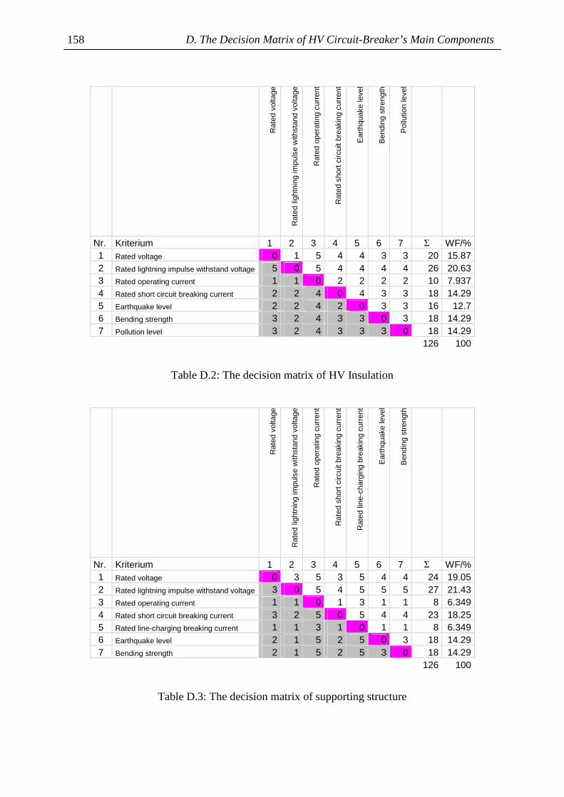
D. The Decision Matrix of HV Circuit-Breaker’s Main Components 158
Rat
ed v
olta
ge
Rat
ed li
ghtn
ing
impu
lse
with
stan
d vo
ltage
Rat
ed o
pera
ting
curr
ent
Rat
ed s
hort
circ
uit b
reak
ing
curr
ent
Ear
thqu
ake
leve
l
Ben
ding
str
engt
h
Pol
lutio
n le
vel
Nr. Kriterium 1 2 3 4 5 6 7 Σ WF/% 1 Rated voltage 0 1 5 4 4 3 3 20 15.87 2 Rated lightning impulse withstand voltage 5 0 5 4 4 4 4 26 20.63 3 Rated operating current 1 1 0 2 2 2 2 10 7.937 4 Rated short circuit breaking current 2 2 4 0 4 3 3 18 14.29 5 Earthquake level 2 2 4 2 0 3 3 16 12.7 6 Bending strength 3 2 4 3 3 0 3 18 14.29 7 Pollution level 3 2 4 3 3 3 0 18 14.29
126 100
Table D.2: The decision matrix of HV Insulation
Rat
ed v
olta
ge
Rat
ed li
ghtn
ing
impu
lse
with
stan
d vo
ltage
Rat
ed o
pera
ting
curr
ent
Rat
ed s
hort
circ
uit b
reak
ing
curr
ent
Rat
ed li
ne-c
harg
ing
brea
king
cur
rent
Ear
thqu
ake
leve
l
Ben
ding
str
engt
h
Nr. Kriterium 1 2 3 4 5 6 7 Σ WF/% 1 Rated voltage 0 3 5 3 5 4 4 24 19.05 2 Rated lightning impulse withstand voltage 3 0 5 4 5 5 5 27 21.43 3 Rated operating current 1 1 0 1 3 1 1 8 6.349 4 Rated short circuit breaking current 3 2 5 0 5 4 4 23 18.25 5 Rated line-charging breaking current 1 1 3 1 0 1 1 8 6.349 6 Earthquake level 2 1 5 2 5 0 3 18 14.29 7 Bending strength 2 1 5 2 5 3 0 18 14.29
126 100
Table D.3: The decision matrix of supporting structure

D. The Decision Matrix of HV Circuit-Breaker’s Main Components 159
Rat
ed v
olta
ge
Rat
ed o
pera
ting
curr
ent
Rat
ed s
hort
circ
uit b
reak
ing
curr
ent
Firs
t pol
e-to
-cle
ar fa
ctor
Rat
ed li
ne-c
harg
ing
brea
king
cur
rent
Rat
ed o
pera
ting
sequ
ence
Tem
pera
ture
cla
ss
Cla
ssifi
catio
n: n
umbe
r of
ope
ratio
n
Ear
thqu
ake
leve
l
Rat
e of
Ris
e of
Rec
over
y V
olta
ge (
RR
RV
)
Nr. Kriterium 1 2 3 4 5 6 7 8 9 10 Σ WF/% 1 Rated voltage 0 5 4 4 5 4 3 5 5 5 40 14.81 2 Rated operating current 1 0 1 2 3 1 1 1 3 2 15 5.556 3 Rated short circuit breaking current 2 5 0 5 5 4 3 4 5 5 38 14.07 4 First pole-to-clear factor 2 4 1 0 4 1 1 2 3 3 21 7.778
5 Rated line-charging breaking current 1 3 1 2 0 1 1 1 1 1 12 4.444
6 Rated operating sequence 2 5 2 5 5 0 3 4 5 5 36 13.33 7 Temperature class 3 5 3 5 5 3 0 4 5 5 38 14.07 8 Classification: number of operation 1 5 2 4 5 2 2 0 4 4 29 10.74 9 Earthquake level 1 3 1 3 5 1 1 2 0 2 19 7.037 10 Rate of Rise of Recovery Voltage 1 4 1 3 5 1 1 2 4 0 22 8.148 270 100
Table D.4: The decision matrix of drive


E. Zusammenfassung in Deutsch 161
Appendix E Zusammenfassung in Deutsch
Die Hauptziele der Arbeit sind Risiko Analyse der Leistungsschalter, Entwicklung der
Wahrscheinlichkeitsmodelle, Aufstellung der Kostenstruktur und Aufbau optimierter
Instandhaltungsmaßnahmen. Normalerweise werden die Instandhaltungsmaßnahmen an
Leistungsschalter nach Hersteller-Richtlinien und Erfahrungen des Betreibers durchgeführt.
Dieses Verfahren ist noch nicht überprüft worden, ob es leistungsfähig und kosteneffizient ist.
Obwohl es viel Literatur über optimierte Instandhaltungsmaßnahmen gibt, stellen die meisten
Beiträge nur Ideen und mathematische Modelle ohne Zusammenhang mit einer Datenbank
vor. Es ist daher eine Herausforderung, die Zuverlässigkeit und Instandhaltungs-Strategie im
Zusammenhang mit einer Datenbank zu untersuchen.
Diese Dissertation ist aus drei Hauptteilen zusammengesetzt. Im ersten Teil wird „Failure
Modes and Effects Analysis (FMEA)“ vorgestellt, damit das Risiko der Komponenten
festgelegt werden können. Der zweite Teil behandelt die Wahrscheinlichkeitsmodelle, um die
Zuverlässigkeit und Entwicklung der Fehler zu erforschen. Im letzten Teil wird die
Kostenstruktur aufgestellt. Außerdem werden optimierte Instandhaltungsmaßnahmen während
der Betriebszeit und Alterungszeit vorgestellt. Auf Grundlage der umfangreichen
Betriebsmittel-Datenbank des Instituts für Elektrische Energieversorgung der TU Darmstadt
ist es möglich, alle Teile durchzuführen.
Das Ergebnis der FMEA-Methode repräsentiert, dass alle Komponenten im niedrigen und
mittleren Risiko-Bereich liegen. Um das Risiko der Komponenten im mittleren Bereich zu
reduzieren, sollten verbesserte Instandhaltungsmaßnahmen zum Einsatz gebracht werden. Mit
Hilfe des „Treeing-und-Cascading-Reliability-Model“-Diagramm ist es möglich
herauszufinden, wann die folgenden Fehler auftreten und mit welcher Wahrscheinlichkeit.
Das Markov-Modell ist ein Wahrscheinlichkeitsmodell, um die Zuverlässigkeit einzelner
Komponenten zu finden. Die Kostenstruktur ist nützlich für Designer, um optimale
Leistungsschalter für verschiedene Anwendungen zu planen. Die Instandhaltung während der
Betriebzeit wird mit Hilfe der Fehlerrate und der optimalen Instandhaltungsfrequenz
durchgeführt. Während der Alterungszeit wird die optimale Instandhaltung mit Hilfe der
Weibull-Verteilung und eines zeitorientierten Instandhaltungsmodells vorgestellt. Schließlich
kann die optimale Zeit zum Austausch eines Leistungsschalters berechnet werden.

Lebenslauf
Name Phuwanart Choonhapran
Geburtsdatum 19. Juni 1976
Geburtsort Bangkok, Thailand
Staatsangehörigkeit Thailändisch
Familienstand ledig
Ausbildung
Schulbildung
1982 – 1988 Grundschule: Reawvadee, Bangkok
1988 – 1991 Gymnasium: Chulalongkorn University Demonstration
Secondary, Bangkok
1991 – 1993 Gynasium: Triam Udom Suksa, Bangkok
Hochschulstudium
1993 – 1997 Studium der Elektrotechnik am King Mongkut’s
Institute of Technology, Ladkrabang, Bangkok
Juni 1997 Abschluss: Bachelor of Engineering
1997 – 2001 Studium der Elektrotechnik an der Chulalongkorn
University, Bangkok
1999 – 2000 Studium der Elektrotechnik an der University of New
South Wales, Sydney, Australien
März 2000 Abschluss: Master of Engineering Science, University
of New South Wales
Juni 2001 Abschluss: Master of Engineering, Chulalongkorn
University
Berufserfahrung
2000 – 2002 Mitarbeiter von Office of Atomic Energy for Peace
(OAEP), Bangkok
2003 – 2007 Wissenschaftlicher Mitarbeiter am Institut für
Elektrische Energieversorgung, Technische Universität
Darmstadt