Applications of Emergent Computation in Reaction-Diffusion CNNs for Image Processing

Radu Dogaru Natural Computing Laboratory, Dept. of Applied Electronics and Information Engineering

University “Politehnica” of Bucharest, Romania Bucharest, Romania

e-mail: radu_d@ieee.org

Abstract—The possibility to exploit emergent computation in a naturally inspired complex network, namely the reaction-diffusion cellular nonlinear network (RD-CNN), is investigated. The particular application under focus is image processing. It is shown that by implementing a simplified discrete-time model and by using the local activity theory to locate potentially useful regions in the huge parameter space, many useful image processing tasks may be performed in reasonable execution time. Such tasks may include but are not limited to: feature extraction, image enhancement, noise removal, pattern formation, etc. A framework is provided for a systematic design allowing the identification of useful genes (sets of parameters) associated with meaningful image processing tasks.

Keywords- nonlinear dynamics; reaction-diffusion systems; cellular nonlinear networks; nonlinear image processing; emergent computation

I. INTRODUCTION The term “reaction-diffusion” was introduced 50 years

ago in relationship with a partial differential equation (PDE) model often used to model various phenomena, mostly those with biological relevance. They are mostly related with pattern formation (e.g. Turing patterns [1]) and the emergence of spatio-temporal waves. Later [2] Chua introduced reaction-diffusion models within the unified approach of the cellular nonlinear networks [3] while considering a spatial discretization on a cellular grid analogous to a resistive grid (as in Figure 1). Reaction in the RD-CNN model is associated with multi-ports injecting currents in the nodes of various layers of the resistive grid while diffusion effects are modeled as currents flowing to the neighboring cells through grid resistors connecting the cells. Lack of diffusion corresponds to a collection of uncoupled cells with no emergent dynamics. Consequently, interesting spatio-temporal dynamics occurs only when non-zero diffusion coefficients (finite positive resistors in the resistive grids) are provided.

In [4], one of the first design for emergence theory was proposed generalizing some theorems from circuit theory to the RD-CNN model. This theory, applicable mostly for 2-layers RD-CNNs and dubbed local activity theory takes advantage of the resistive grid approach and expands the classical theory of stability by adding supplementary conditions for passivity (activity means that the cell is not

passive). The main result of this theory is the following: No emergent behavior is possible in RD-CNN systems with their uncoupled cells being passive in all their equilibrium points. Observe that passivity as well as stability can be tested for a given cell dynamical system (usually a simple 2-dimensional nonlinear system) around equilibrium points (hence the word local meaning linearization around equilibrium, in local activity). Consequently, this theory gives no prediction about the values for the diffusion coefficients but it still allows discarding a large volume of the parameter space where the cell is passive.

Figure 1. The resistive grid model of a RD-CNN

In recent years there is a tremendous interest in reaction-diffusion systems, mostly from a modeling perspective. As shown in [5][6][7] where the theory of local activity was first applied to several well known types of systems (i.e. the FitzHugh-Nagumo model of nervous excitability, and the Brusselator model for a chemical reaction), a particular region called “edge of chaos” (cells are both locally active and stable in at least one equilibrium point) was easily identified. Picking parameters from that region proved the assumptions of the local activity theory valid and of practical relevance. So far most research in the area of RD-CNN deals

2013 19th International Conference on Control Systems and Computer Science

978-0-7695-4980-4/13 $26.00 © 2013 IEEE

DOI 10.1109/CSCS.2013.39

370

2013 19th International Conference on Control Systems and Computer Science

978-0-7695-4980-4/13 $26.00 © 2013 IEEE

DOI 10.1109/CSCS.2013.39

370

with modeling applications and with complex wave computing. Reaction diffusion systems were recognized as interesting computing devices [8]. Still there is a lot of un-explored potential for their use in image processing, similarly to the standard cellular neural network (CNN) [9], widely used as visual microprocessors with parallel and highly efficient implementations. The advantage of using RD-CNNs for building image processors stands in their inherent parallelism and very simple coupling (resistive grids). Several analogue chips were already proposed in the literature [10][11][12][13], although we consider that from a practical point of view, digital models would be better. Speeding-up such models using GPU/CUDA approaches [14] are also convenient solutions in terms of good ratios between performances and costs. In this paper we propose the development of a RD-CNN processor suitable for digital implementations (PC, GPU cards, FPGAs, etc.) aiming to identify several useful image processing tasks resulting from choosing the parameters (genes) within emergence maps obtained by applying the local activity theory. Section II introduces the simplified, discrete-time RD-CNN model as image processor. A reminder of the local activity techniques for locating emergent behaviors is given in Section III. Section IV presents some representative genes and their associated image processing tasks. Feature extraction, image enhancement, noise removal and pattern generation are considered.

II. THE RD-CNN PROCESSOR APPLIED FOR IMAGE PROCESSING

A. The continuous time RD-CNN model The mathematical model of the RD-CNN in Fig.1 is

particularized next, for the 2-layers excitability model of FitzHugh Nagumo [15][7]. Consequently, there are two diffusion coefficients D1 and D2 defining the coupling.

( ) [ ]jijijijijijijiji uuuuuDGvuf

dtdu

,,1,11,1,1,,1, 4,, −++++= +−−+ (1)

( ) [ ]jijijijijijijiji uuuuuDGvuf

dtdv

,,1,11,1,2,,2, 4,, −++++= +−−+

(2)

with the nonlinear functions given by the following particular formulae (specific for the FitzHugh-Nagumo model):

( ) vucuvuf −−= 331

1 , (3)

( ) ( )abvuevuf +−−=,2 (4)

The set of cell parameters is called a gene and in this particular case, ],,,[ ebac=G . Following the original notation in [7] the c parameter is sometimes dubbed alpha

and e is dubbed eps. A much larger variety of RD-CNNs may be considered by simply changing the two nonlinear cells associated with the uncoupled cell. A prerequisite for spatio-temporal emergence is the existence of at least one nonlinear function defining the reaction, this is the case of equation (3) in our case, plotted in Fig. 2 for various c parameters.

Figure 2. Plots of the equation ( ) 0,1 =vuf for different values of

parameter c.

Such a model is equivalent to an excitable sheet where images are applied as initial states and the spatio-temporal dynamics developing performs various types of computations (image processing). Each pixel of an image corresponds to a state variable in one of the RD-CNN layers. There are many possibilities to control the nature of the image processing.

B. The discrete-time RD-CNN as image processor Integrating the ordinary differential equation (ODE) system associated with the RD-CNN requires the use of specific numeric methods such as Runge-Kutta. Let us consider such an example, where an initial state random image with N=100x100 pixels (generated using the rand function in Matlab) has to be processed. In Figure 3 the resulting image on the plane “u” is given for both the continuous-time model and the discrete-time model to be introduced.

Figure 3. The output image from a RD-CNN processor with parameters (a=0.07, b=2.3, eps=-0,1, alpha=1, D1=0.3, D2=2). Left: resulted from an integration of the ODE system using ode23 Matlab function; Right: resulted from a simplified discrete-time model based on Euler approximation. A 10-times reduction of the computation time is observed, while the output image is not affected in its essential features.

Note that the final result is almost the same, although the Runge-Kutta integration lasts 10 times more than in the case of the simplified, discrete-time model using the simple Euler approximation of the time derivatives:

Since image processing mostly exploits the equilibrium type of spatio-temporal dynamics, such simplifications are expected to have no major influence on the final results.

371371

Consequently, in the following the RD-CNN processor is implemented according to the following formulae:

( )( ) ( )[ ]( ) ( )[ ]

������

�

�

=

=

−++++Δ+=

−++++Δ+=

=

==

+

+

+−−++

+−−++

jiji

jiji

jijijijijijijijiji

jijijijijijijijiji

jijijiji

vv

uu

vvvvvDvuftvv

uuuuuDvuftuu

jiTt

xvxu

,,

,,

,1,1,,1,11,,2,,

,1,1,,1,11,,1,,

,,,,

4,

4,

, cells allfor and ,...1for

; ; λλ (5)

The output (processed images) are given by the jiu , and

jiv , state variables associated with the two layers, scaled accordingly. In the above, the same functions and parameters as in the original continuous-time model are used. In addition to the cell parameters and diffusion coefficients, two more parameters are introduced by this model: The number of iterations T corresponds to a period of time tTΔ of the continuous time model. The output depends on T so it may be additionally tuned to get the desired effect. On the other hand, numerical simulations show that if crittt Δ>Δ , the overall system becomes unstable. From various experiments it turns out that 12.0≅Δ critt , consequently in the next we will consider 1.0=Δt if not specified otherwise. It is interesting to note that standard gray level images assume their pixels [ ]1,1, −∈jix . The gain parameter λ may also influence the dynamics and the output image. If not specified otherwise, 5.0=λ .

The image processor described by equation (5) may be conveniently implemented not only in any standard computing language but also on high computing platforms such as GPU/CUDA or OpenCL or FPGAs. Various solutions for implementing cellular automata on such platforms are recently presented in the literature (e.g. [14][16]), making it easily to adjust them to the model (5) which has many similarities to any continuous state cellular automaton.

Figure 4 presents the dynamics of both “u” and “v” layers for T=200 and for some face image cropped from one of the faces in the database [17]. Note that the dynamics may be stopped at any time step, depending on the desired processing effect.

Figure 4. The dynamics of the RD-CNN image processor (5) for T=200 iterations. The cell parameters were chosen in the “edge of chaos” region.

III. LOCATING EMERGENT BEHAVIORS, GENES ASSOCIATED TO IMAGE PROCESSING TASKS

As discussed above, there are many parameters influencing the dynamics of the RD-CNN and consequently the nature of the image processing. The theory of local activity provides a convenient and computationally tractable method to generate maps in the parameter space defining qualitatively different regions. The method was first applied for the FitzHugh Nagumo model [5] and the details are presented in that work. It is important to note that the entire analysis is performed to the uncoupled cell i.e. the 2-dimensional nonlinear dynamical system (1)–(4) with null diffusion coefficients: (i) First, the equilibrium points iQ are determined, i.e. 2-dimensional [ ]vu, vectors for which

( ) ( ) 0,, 21 == vufvuf . In our case it is possible to have 1 or 3 equilibrium points; (ii) Arround each equilibrium point the nonlinear ordinary differential equation is linearized, i.e. approximated with a linear ODE system in given by:

���

���

��

��

�=��

�

���

vu

aaaa

dtdvdtdu

2221

1211

//

(6)

where ufa

∂∂= 1

11 , vfa

∂∂= 1

12 , ufa

∂∂= 2

11 , vfa

∂∂= 2

11 are

evaluated for the particular equilibrium point; (iii) Finally, classical results of stability theory and more recent results of passivity theory [3] are applied to test whether the particular equilibrium is in one of the following situations: SA: (stable and active)

( )( ) ( )0 AND 0 AND 4 OR 0 22112221122 ><+<> DELTaaaaa

P: (stable and passive) ( ) ( )( ) 4 AND 0a 2

2112221122 aaaa +≥< UA: (unstable and active) None of the above conditions is satisfied.

The above test is detailed [5] based on the local activity theory [3][4] for the case of two positive diffusion coefficients. If 02 =D , the tests are slightly different [5] and will lead to a much larger passivity region. In other words, more interesting emergent behaviors are expected when both

21, DD are non-zero. In the above ( )2211 aaT += is the trace and 21122211 aaaaDEL −= is the determinant of the Jacobian matrix in (6).

One may prescribe all gene parameters except two of them and apply the above tests with a given resolution M for some predefined ranges. For instance one may choose:

( )Mibbbbi minmaxmin −+= and ( )

Mj

aaaa j minmaxmin −+=

Each particular set of parameters ( )ji ab , will be projected in an image (map) dubbed next an emergence map using a color code (Figure 5) associated with the types of

372372

stability/passivity and number of equilibrium points found by the above test.

Figure 5. Color code (type number above) associated with various types

of stability/passivity and number of equilibria for a givem set of parameters.

Such maps are extremely useful since they allow the rapid location of interesting points, based on the local activity theory and its corollaries. For instance, the blue region associated to passivity will be avoided because in this case the theory guarantees that no emergent behaviors occur in the network of cells. It was also determined that in order to achieve emergent but stable behaviors (of interest for image processing dynamics), parameter cells must be selected from the type 2,6,7 or 10 regions (i.e. having at least one stable and active equilibrium point). On the opposite, wave-type dynamics is favored by the selection of parameter points in the UA (unstable and active) regions of the parameter space (5,6,7,9,10,13). It was also found that most interesting emergent behaviors occur taking cell parameter points from those regions (type 6 to 13) associated with a maximum number of equilibrium points (3 in our case).

Let us consider such a map in Figure 6. In the next section several points in this section of the parameter space will be further investigated by effectively running the RD-CNN image processor (5). Other maps may be also considered in order to diversity the image processing tasks.

Figure 6. Emergence map for a specified region of the a,b parameters.

IV. IMAGE PROCESSING AND PATTERN FORMATION In using emergent computation (often associated with a

surprise effect) is difficult to have a design approach that is similar to the spatial filter design (given a bandwidth and other characteristics, one can calculate the parameters of the filtering system). Consequently, the approach is rather

evolutionary: one picks a gene from the parameter space and observes the kind of dynamics for various types of images. One may select interesting processing functions and fill in a catalogue containing many entries using the model of [18] for the standard CNN. Such an entry would give the gene, other specific parameters (e.g. T or λ ) a linguistic description (e.g. “short edges enhancement”) and several examples.

A. Feature enhancement Several crops (denoted as images A to E) from face

images of the [17] database were considered as inputs in the following experiments. Also, a retinal fundus image F from [19] is considered here. All these input images were normalized to gray scale images with 5.0=λ (Figure 7).

Figure 7. Test images used as inputs to the RD-CNN image processor (5)

in order to identify meaningflul genes.

If not specified otherwise T=200 and 1.0=Δt . Let first consider the cell parameter point A:

1 ,1.0 ,2 ,25.0 =−==−= ceba in emergence section in Fig.6. This point was selected in a region of type 7 with 3 equilibrium points, 2 of which are stable. As seen in Figure 7, while tuning the D1 coefficients one may obtain various kind of features from the initial state images. Such features may be of interest in various face recognition algorithms

373373

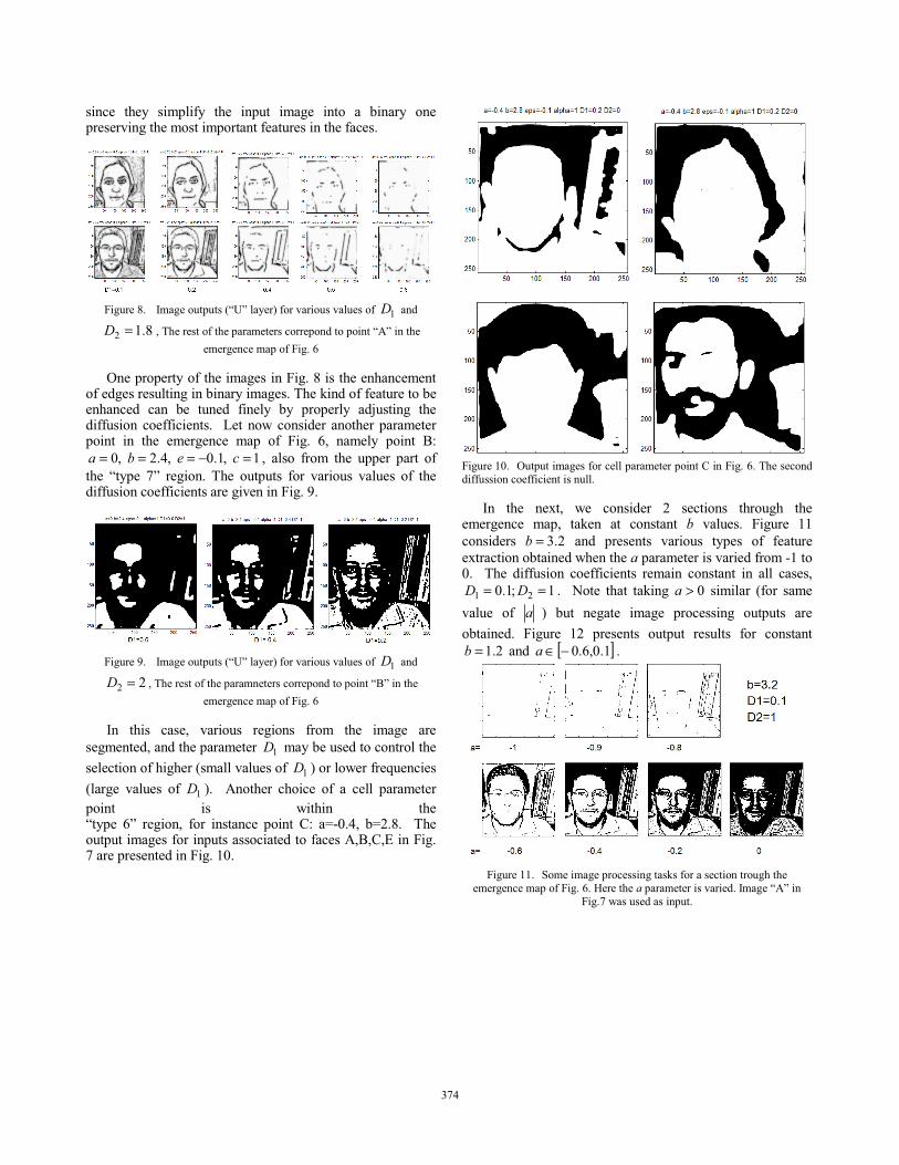
since they simplify the input image into a binary one preserving the most important features in the faces.

Figure 8. Image outputs (“U” layer) for various values of 1D and

8.12 =D , The rest of the parameters correpond to point “A” in the emergence map of Fig. 6

One property of the images in Fig. 8 is the enhancement of edges resulting in binary images. The kind of feature to be enhanced can be tuned finely by properly adjusting the diffusion coefficients. Let now consider another parameter point in the emergence map of Fig. 6, namely point B:

1 ,1.0 ,4.2 ,0 =−=== ceba , also from the upper part of the “type 7” region. The outputs for various values of the diffusion coefficients are given in Fig. 9.

Figure 9. Image outputs (“U” layer) for various values of 1D and

22 =D , The rest of the paramneters correpond to point “B” in the emergence map of Fig. 6

In this case, various regions from the image are segmented, and the parameter 1D may be used to control the selection of higher (small values of 1D ) or lower frequencies (large values of 1D ). Another choice of a cell parameter point is within the “type 6” region, for instance point C: a=-0.4, b=2.8. The output images for inputs associated to faces A,B,C,E in Fig. 7 are presented in Fig. 10.

Figure 10. Output images for cell parameter point C in Fig. 6. The second diffussion coefficient is null.

In the next, we consider 2 sections through the emergence map, taken at constant b values. Figure 11 considers 2.3=b and presents various types of feature extraction obtained when the a parameter is varied from -1 to 0. The diffusion coefficients remain constant in all cases,

1;1.0 21 == DD . Note that taking 0>a similar (for same value of a ) but negate image processing outputs are obtained. Figure 12 presents output results for constant

2.1=b and [ ]1.0,6.0−∈a .

Figure 11. Some image processing tasks for a section trough the

emergence map of Fig. 6. Here the a parameter is varied. Image “A” in Fig.7 was used as input.

374374

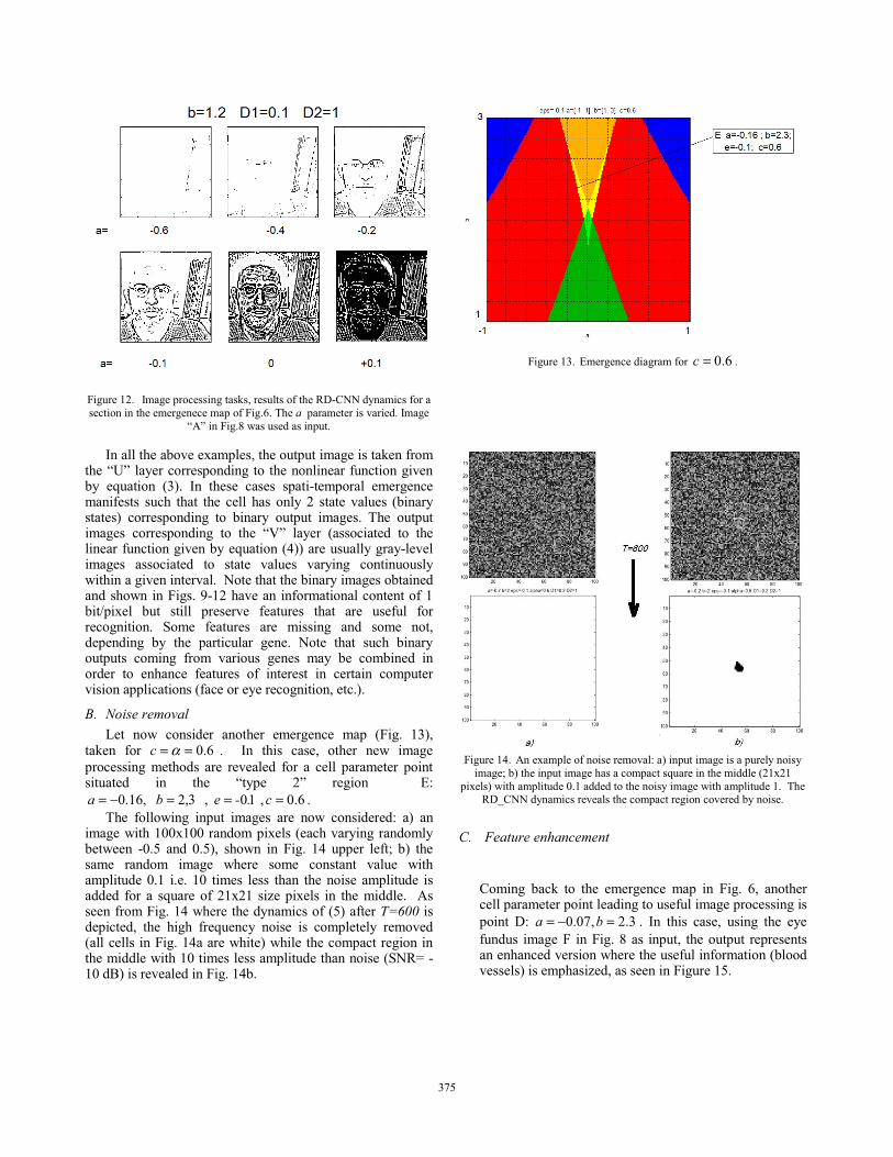
Figure 12. Image processing tasks, results of the RD-CNN dynamics for a section in the emergenece map of Fig.6. The a parameter is varied. Image

“A” in Fig.8 was used as input.

In all the above examples, the output image is taken from the “U” layer corresponding to the nonlinear function given by equation (3). In these cases spati-temporal emergence manifests such that the cell has only 2 state values (binary states) corresponding to binary output images. The output images corresponding to the “V” layer (associated to the linear function given by equation (4)) are usually gray-level images associated to state values varying continuously within a given interval. Note that the binary images obtained and shown in Figs. 9-12 have an informational content of 1 bit/pixel but still preserve features that are useful for recognition. Some features are missing and some not, depending by the particular gene. Note that such binary outputs coming from various genes may be combined in order to enhance features of interest in certain computer vision applications (face or eye recognition, etc.).

B. Noise removal Let now consider another emergence map (Fig. 13),

taken for 6.0== αc . In this case, other new image processing methods are revealed for a cell parameter point situated in the “type 2” region E:

6.0, 10 , 3,2 ,16.0 ===−= c.-eba . The following input images are now considered: a) an

image with 100x100 random pixels (each varying randomly between -0.5 and 0.5), shown in Fig. 14 upper left; b) the same random image where some constant value with amplitude 0.1 i.e. 10 times less than the noise amplitude is added for a square of 21x21 size pixels in the middle. As seen from Fig. 14 where the dynamics of (5) after T=600 is depicted, the high frequency noise is completely removed (all cells in Fig. 14a are white) while the compact region in the middle with 10 times less amplitude than noise (SNR= -10 dB) is revealed in Fig. 14b.

Figure 13. Emergence diagram for 6.0=c .

Figure 14. An example of noise removal: a) input image is a purely noisy

image; b) the input image has a compact square in the middle (21x21 pixels) with amplitude 0.1 added to the noisy image with amplitude 1. The

RD_CNN dynamics reveals the compact region covered by noise.

C. Feature enhancement Coming back to the emergence map in Fig. 6, another cell parameter point leading to useful image processing is point D: 3.2,07.0 =−= ba . In this case, using the eye fundus image F in Fig. 8 as input, the output represents an enhanced version where the useful information (blood vessels) is emphasized, as seen in Figure 15.

375375

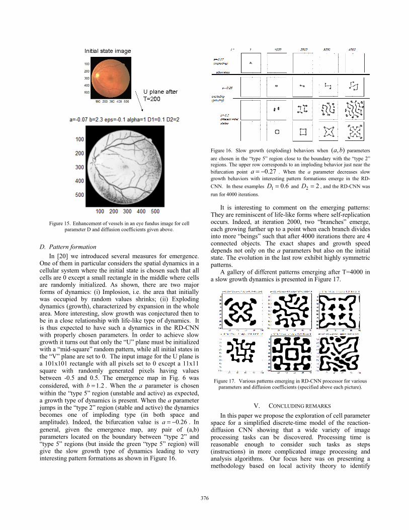
Figure 15. Enhancement of vessels in an eye fundus image for cell

parameter D and diffusion coefficients given above.

D. Pattern formation In [20] we introduced several measures for emergence.

One of them in particular considers the spatial dynamics in a cellular system where the initial state is chosen such that all cells are 0 except a small rectangle in the middle where cells are randomly initialized. As shown, there are two major forms of dynamics: (i) Implosion, i.e. the area that initially was occupied by random values shrinks; (ii) Exploding dynamics (growth), characterized by expansion in the whole area. More interesting, slow growth was conjectured then to be in a close relationship with life-like type of dynamics. It is thus expected to have such a dynamics in the RD-CNN with properly chosen parameters. In order to achieve slow growth it turns out that only the “U” plane must be initialized with a “mid-square” random pattern, while all initial states in the “V” plane are set to 0. The input image for the U plane is a 101x101 rectangle with all pixels set to 0 except a 11x11 square with randomly generated pixels having values between -0.5 and 0.5. The emergence map in Fig. 6 was considered, with 2.1=b . When the a parameter is chosen within the “type 5” region (unstable and active) as expected, a growth type of dynamics is present. When the a parameter jumps in the “type 2” region (stable and active) the dynamics becomes one of imploding type (in both space and amplitude). Indeed, the bifurcation value is 26.0−=a . In general, given the emergence map, any pair of (a,b) parameters located on the boundary between “type 2” and “type 5” regions (but inside the green “type 5” region) will give the slow growth type of dynamics leading to very interesting pattern formations as shown in Figure 16.

Figure 16. Slow growth (exploding) behaviors when ),( ba parameters are chosen in the “type 5” region close to the boundary with the “type 2” regions. The upper row corresponds to an imploding behavior just near the bifurcation point 27.0−=a . When the a parameter decreases slow growth behaviors with interesting pattern formations emerge in the RD-CNN. In these examples 6.01 =D and 22 =D , and the RD-CNN was run for 4000 iterations.

It is interesting to comment on the emerging patterns: They are reminiscent of life-like forms where self-replication occurs. Indeed, at iteration 2000, two “branches” emerge, each growing further up to a point when each branch divides into more “beings” such that after 4000 iterations there are 4 connected objects. The exact shapes and growth speed depends not only on the a parameters but also on the initial state. The evolution in the last row exhibit highly symmetric patterns.

A gallery of different patterns emerging after T=4000 in a slow growth dynamics is presented in Figure 17.

Figure 17. Various patterns emerging in RD-CNN processor for various

parameters and diffusion coefficients (specified above each picture).

V. CONCLUDING REMARKS In this paper we propose the exploration of cell parameter

space for a simplified discrete-time model of the reaction-diffusion CNN showing that a wide variety of image processing tasks can be discovered. Processing time is reasonable enough to consider such tasks as steps (instructions) in more complicated image processing and analysis algorithms. Our focus here was on presenting a methodology based on local activity theory to identify

376376

regions in the cell parameter space such that taking points in these regions gives a good chance to discover a meaningful image processing task. Comparison with other specific image processing techniques reported in the literature (e.g. eye fundus enhancement) is a subject of further research. For instance, [21] reports several interesting image processing tasks in a cellular nonlinear network (CNN) based on universal binary neurons. Their technique involves learning of the image processing task in a novel neuron model acting as a filter in a local neighborhood of the CNN. Our approach involves no learning (and its associated time processing) while it is based on identifying useful cell parameter points using local activity theory. Moreover, most of the image processing tasks in CNN including [21] are based on a strict processing of the neighbor pixels (e.g. 3x3 neighboring pixels). Instead, the RD-CNN with cells operated in the local activity region presents a global spreading effect i.e. processing is equivalent to much larger neighborhoods while the implementation maintains a very simple and consequently fast processing architecture.

Further research is expected to reveal even more interesting image processing tasks while changing the nonlinear reaction module and exploring wider regions of the emergence maps.

REFERENCES

[1] A. M. Turing, The Chemical Basis of Morphogenesis, Phil. Trans. Roy. Soc. Lond., 237, 37-72 (1952)

[2] L. O. Chua, M. Hasler, G. S. Moschytz, and J. Neirynck, “Autonomous cellular neural networks: a unified paradigm for pattern formation and active wave propagation,” IEEE Trans. Circuits Syst. I, Fundam. Theory Appl., vol. 42, no. 10, pp. 559–577, Oct. 1995.

[3] L. O. Chua, “CNN: A paradigm for complexity,” in Visions of Nonlinear Science in the 21st Century. Eds. Singapore: World Scientific, 1999, vol. 26.

[4] L. O. Chua, “CNN: a Vision of Complexity ”, International Journal of Bifurcation and Chaos, Vol. 7, No. 10, pp. 2219-2425, 1997.

[5] R. Dogaru and L. O. Chua, "Edge of Chaos and Local Activity Domain of FitzHugh-Nagumo Equation", in International Journal of Bifurcation and Chaos (IJBC), Volume: 8, Issue: 2(1998) pp. 211-257.

[6] R. Dogaru and L. O. Chua, "Edge of Chaos and Local Activity Domain of the Brusselator CNN", International Journal of Bifurcation and Chaos, Vol. 8, No. 6 (1998) 1107–1130.

[7] R. Dogaru, Universality and Emergent Computation in Cellular Neural Networks, World Scientific, Singapore, 2003.

[8] A. Adamatzky, B. De Lacy Costello, and T. Asai, Reaction-diffusion Computers, Elsevier, 2005

[9] L. Chua and T. Roska, Cellular neural networks and visual computing - Foundations and applications, Cambridge University Press, 2001.

[10] K. Karahaliloglu and S. Balk�r, "Bio-Inspired Compact Cell Circuit for Reaction–Diffusion Systems", IEEE Transactions on Circuits and Systems—II: Express Briefs, Vol. 52, No. 9, September 2005, pp. 558-562

[11] T. Serrnao-Gotarredona and B. Linares-Barranco, “Log-domain implementation of complex dynamics reaction diffusion neural networks,” IEEE Trans. Neural Netw., vol. 14, no. 9, pp. 1337–1355, Sep. 2003.

[12] V. Bonaiuto, A. Maffucci, G. Miano, M. Salerno, F. Sargeni, and C. Visone,“Design of a cellular nonlinear network for analogue

simulation of reaction-diffusion PDEs,” in Proc. ISCAS, vol. 3, 2000, pp. 431–434.

[13] Y. Matsubara, T. Asai, T. Hirose and Y. Amemiya, “Reaction-diffusion chip implementing excitable lattices with multiple-valued cellular automata”, in IEICE Electron. Express 1 (2004) 248-252.

[14] K.V. Kalgin, “Implementation of algorithms with a fine-grained parallelism on GPUs”, Numerical Analysis and Applications, Vol.4, No.1, pp 46-55, 2011.

[15] R. A. Fitzhugh, “Impulses and physiological states in theoretical models of nerve membrane,” Biophys. J., vol. 1, pp. 445–466, 1961.

[16] L. Dematté, and D. Prandi, “GPU computing for systems biology”, Briefings in Bioinformatics. 11, 3 (May. 2010), 323-333.

[17] Georgia Tech Face Database, available from http://www.anefian.com/research/gt_db.zip

[18] Software Library for Cellular Wave Computing Engines in an era of kilo-processor chips, Version 3.1, 2010; Available from http://cnn-technology.itk.ppke.hu/Template_library_v3.1.pdf

[19] J.J. Staal, M.D. Abramoff, M. Niemeijer, M.A. Viergever, B. van Ginneken, "Ridge based vessel segmentation in color images of the retina", IEEE Transactions on Medical Imaging, 2004, vol. 23, pp. 501-509. Available from: http://www.isi.uu.nl/Research/Databases/DRIVE/

[20] R. Dogaru, Systematic design for emergence in cellular nonlinear networks – with applications in natural computing and signal processing, Springer-Verlag, Berlin Heidelberg, 2008.

[21] I. Aizenberg, C. Butakoff, "Image Processing Using Cellular Neural Networks Based on Multi-Valued and Universal Binary Neurons", J. VLSI Signal Process. Syst., vol. 32, nos. 1–2, pp. 169–188, Aug.–Sep. 2002.

377377