Applications of Convolutional Neural Networks to Facial ...
148
COOPER UNION FOR THE ADVANCEMENT OF SCIENCE AND ART ALBERT NERKEN SCHOOL OF ENGINEERING Applications of Convolutional Neural Networks to Facial Detection and Recognition for Augmented Reality and Wearable Computing by Christopher Mitchell A thesis submitted in partial fulfillment of the requirements for the degree of Master of Engineering May 3, 2010 Advisor Prof. Carl Sable
Transcript of Applications of Convolutional Neural Networks to Facial ...

COOPER UNION FOR THE ADVANCEMENT OF SCIENCE AND ART
ALBERT NERKEN SCHOOL OF ENGINEERING
Applications of Convolutional Neural
Networks to Facial Detection and
Recognition for Augmented
Reality and Wearable Computing
by
Christopher Mitchell
A thesis submitted in partial fulfillment
of the requirements for the degree of
Master of Engineering
May 3, 2010
Advisor
Prof. Carl Sable

COOPER UNION FOR THE ADVANCEMENT OF SCIENCE AND ART
ALBERT NERKEN SCHOOL OF ENGINEERING
This thesis was prepared under the direction of the Candidate’s Thesis Ad-visor and has received approval. It was submitted to the Dean of the Schoolof Engineering and the full Faculty, and was approved as partial fulfillment ofthe requirements for the degree of Master of Engineering.
Dr. Simon Ben AviDean, School of Engineering
Prof. Carl SableCandidate’s Thesis Advisor

Acknowledgments
This project could not have been completed without the guidance and support
of family, friends, and professors. Professor Carl Sable has been a source of
tireless and patient guidance, advisement, and knowledge; his countless days of
proofreading, project ideas, and graduate school admissions advice have been
invaluable. I have reached this point in my career only through the efforts of
many professors, including but certainly not limited to Fred Fontaine, Stuart
Kirtman, Yash Risbud, Jeff Hakner, Hamid Ahmad, Kausik Chatterjee, Gerald
Ryan, Billy Donahue, Chris Lent, and many others. Glenn Gross and Dino
Melendez have shared their expertise and supported my hardware projects for
my five-year career at the Cooper Union. Thanks to S∗ProCom2 and its fellows
and advisors for invaluable hardware support for this and many other projects.
A tip of the hat to Yann LeCun at the Courant Institute of Mathematical
Sciences for his breakthrough work with convolutional neural networks and
his personal guidance in optimizing my implementation.
Many friends have provided their help and support over the years in various
aspects including my thesis, especially Deian Stefan, Dave Nummey, Nick
Powel, Subodh Shrestha, Akshay Anand, Shaurav Garg, Samar Kamat, Tiago
Zeitoune, Tanbera Chowdhury, Kevin Chang, Kwame Wright, Brian Cheung,
and Kenny Lam among many others. Thanks to Jim Kent for his support and
for driving my entrepreneurial spirit. Special thanks go to Nick Cooper for

iv
lending me a compassionate ear over many months of personal and academic
stumbling blocks, as well as a source of many ideas and constructive criticism
for this project. Kudos to Adam Charles for encouraging me to keep a running
progress log as I worked on my thesis, and a salute to the members of Cemetech
for moral support and an impetus to meet my personal deadlines.
Thank you to Chrystina Montuori Sorrentino, for many years of being my
best friend, my confidant, and an unquenchable font of love and support. I owe
her eternal gratefulness for always believing in me and standing at my side.
Finally, thanks to my mother for twenty-three years of hard work, finding the
best educational opportunities for me, encouraging me, and putting up with
transistors, hard drives, and LEGOs strewn across every available surface.
Without her efforts through my childhood and up to the present, including
carefully proofreading this thesis, I would never be where I am today.

Abstract
Facial detection and recognition are among the most heavily researched
fields of computer vision and image processing. However, the computation
necessary for most facial processing tasks has historically made it unfit for
real-time applications. The constant pace of technological progress has made
current computers powerful enough to perform near-real-time image process-
ing and light enough to be carried as wearable computing systems. Facial
detection within an augmented reality framework has myriad applications, in-
cluding potential uses for law enforcement, medical personnel, and patients
with post-traumatic or degenerative memory loss or visual impairments. Al-
though the hardware is now available, few portable or wearable computing
systems exist that can localize and identify individuals for real-time or near-
real-time augmented reality.
The author presents a system design and implementation that performs ro-
bust facial detection and recognition robust to variations in lighting, pose, and
scale. Scouter combines a commodity netbook computer, a high-resolution
webcam, and display glasses into a light and powerful wearable computing
system platform for real-time augmented reality and near-real-time facial pro-
cessing. A convolutional neural network performs precise facial localization, a
Haar cascade object detector is used for facial feature registration, and a Fish-

vi
erface implementation recognizes size-normalized faces. A novel multiscale
voting and overlap removal algorithm is presented to boost face localization
accuracy; a failure-resilient normalization method is detailed that can perform
rotation and scale normalization on faces with occluded or undetectable facial
features. The development, implementation, and positive performance results
of this system are discussed at length.

Contents
Table of Contents vii
List of Figures x
List of Tables xii
1 Introduction 1
2 Tools and Conventions 42.1 APIs and Tools . . . . . . . . . . . . . . . . . . . . . . . . . . . . . . 42.2 Images Used . . . . . . . . . . . . . . . . . . . . . . . . . . . . . . . . 52.3 Conventions . . . . . . . . . . . . . . . . . . . . . . . . . . . . . . . . 6
3 Previous Work 93.1 Facial Recognition Algorithms . . . . . . . . . . . . . . . . . . . . . . 11
3.1.1 PCA and Eigenfaces . . . . . . . . . . . . . . . . . . . . . . . 113.1.2 Linear Subspaces and Fisherfaces . . . . . . . . . . . . . . . . 153.1.3 Hidden Markov Models . . . . . . . . . . . . . . . . . . . . . . 183.1.4 Convolutional Neural Networks . . . . . . . . . . . . . . . . . 183.1.5 Support Vector Machines . . . . . . . . . . . . . . . . . . . . . 19
3.2 Facial Detection Techniques . . . . . . . . . . . . . . . . . . . . . . . 233.2.1 Eigenfaces . . . . . . . . . . . . . . . . . . . . . . . . . . . . . 253.2.2 Eigenfeatures . . . . . . . . . . . . . . . . . . . . . . . . . . . 263.2.3 Haar Classifier . . . . . . . . . . . . . . . . . . . . . . . . . . 263.2.4 Neural Networks and Multilayer Perceptrons . . . . . . . . . . 283.2.5 Convolutional Neural Networks . . . . . . . . . . . . . . . . . 33
3.3 Wearable Computing and Augmented Reality . . . . . . . . . . . . . 443.3.1 Hardware . . . . . . . . . . . . . . . . . . . . . . . . . . . . . 453.3.2 Applications . . . . . . . . . . . . . . . . . . . . . . . . . . . . 48
4 Experimentation and Development 504.1 CNN Development . . . . . . . . . . . . . . . . . . . . . . . . . . . . 51
4.1.1 Initial Implementation . . . . . . . . . . . . . . . . . . . . . . 514.1.2 Multiscale Detection . . . . . . . . . . . . . . . . . . . . . . . 52
vii

CONTENTS viii
4.1.3 The Intel Performance Primitives (IPP) Library . . . . . . . . 544.1.4 Algorithmic Corrections . . . . . . . . . . . . . . . . . . . . . 554.1.5 Classification Algorithm . . . . . . . . . . . . . . . . . . . . . 564.1.6 Final Adjustments . . . . . . . . . . . . . . . . . . . . . . . . 59
4.2 CNN Training . . . . . . . . . . . . . . . . . . . . . . . . . . . . . . . 604.2.1 Preprocessor Development and the Yale B Database . . . . . . 614.2.2 Early Training Performance . . . . . . . . . . . . . . . . . . . 654.2.3 Training Set Expansion and Refinement . . . . . . . . . . . . 674.2.4 Training Process and Parameter Tuning . . . . . . . . . . . . 69
4.3 Evolution of the Overlap Removal Algorithm . . . . . . . . . . . . . . 764.3.1 Simple Overlap Removal . . . . . . . . . . . . . . . . . . . . . 764.3.2 Weighted Overlap Removal . . . . . . . . . . . . . . . . . . . 78
4.4 Eigenfeature Detector Development . . . . . . . . . . . . . . . . . . . 804.4.1 Eigenfeature Basis Extraction . . . . . . . . . . . . . . . . . . 834.4.2 Eigenfeature Detector Implementation . . . . . . . . . . . . . 85
4.5 Haar Cascade Feature Detector Development . . . . . . . . . . . . . . 864.5.1 Face Normalizer . . . . . . . . . . . . . . . . . . . . . . . . . . 89
4.6 Fisherface Recognizer Development . . . . . . . . . . . . . . . . . . . 93
5 Implementation 965.1 Hardware Design . . . . . . . . . . . . . . . . . . . . . . . . . . . . . 97
5.1.1 Computing Platform . . . . . . . . . . . . . . . . . . . . . . . 985.1.2 Display . . . . . . . . . . . . . . . . . . . . . . . . . . . . . . 1005.1.3 Video Capture . . . . . . . . . . . . . . . . . . . . . . . . . . 1015.1.4 Peripherals and Modifications . . . . . . . . . . . . . . . . . . 102
5.2 Software Implementation . . . . . . . . . . . . . . . . . . . . . . . . . 1025.2.1 Facial Detection . . . . . . . . . . . . . . . . . . . . . . . . . . 1035.2.2 Overlap Removal . . . . . . . . . . . . . . . . . . . . . . . . . 1065.2.3 Facial Feature Registration . . . . . . . . . . . . . . . . . . . . 1075.2.4 Facial Normalization . . . . . . . . . . . . . . . . . . . . . . . 1105.2.5 Facial Recognition: Fisherfaces . . . . . . . . . . . . . . . . . 1115.2.6 Secondary Software . . . . . . . . . . . . . . . . . . . . . . . . 112
6 Results and Evaluation 1146.1 Speed and Resource Utilization . . . . . . . . . . . . . . . . . . . . . 1156.2 Face Detection Performance . . . . . . . . . . . . . . . . . . . . . . . 1196.3 Face Recognition Performance . . . . . . . . . . . . . . . . . . . . . . 120
7 Conclusion 123
A Description of Eigentemplates As Convolutions 127
Bibliography 130

CONTENTS ix
Figure 1 A screenshots from the final Scouter face detector and recognizerimplementation.

List of Figures
1 Final Scouter Screenshot . . . . . . . . . . . . . . . . . . . . . . . . . ix
3.1 Types of pose variation . . . . . . . . . . . . . . . . . . . . . . . . . . 103.2 Simple optimal and suboptimal SVM solutions for two-class system . 203.3 Conceptual Haar Features . . . . . . . . . . . . . . . . . . . . . . . . 273.4 Standard neural network architecture . . . . . . . . . . . . . . . . . . 293.5 Lenet-5 CNN Architecture . . . . . . . . . . . . . . . . . . . . . . . . 353.6 CNN Convolutional Layer Structure . . . . . . . . . . . . . . . . . . . 373.7 CNN Subsampling Layer Structure . . . . . . . . . . . . . . . . . . . 383.8 CNN Full Connection Layer Structure . . . . . . . . . . . . . . . . . 393.9 CNN architecture proposed in Vaillant et al. 1994 . . . . . . . . . . . 403.10 CNN architecture proposed in Osadchy et al. 2007 . . . . . . . . . . . 433.11 Client-server models for wearable computing . . . . . . . . . . . . . . 48
4.1 Initial CNN Facial Detector Performance . . . . . . . . . . . . . . . . 564.2 Two-Class Face/Nonface Scores . . . . . . . . . . . . . . . . . . . . . 574.3 CNN Permutation Repair Performance . . . . . . . . . . . . . . . . . 614.4 Sample Positive and Negative Training Image Mutations . . . . . . . 654.5 Sample Results for Six-Category CNN Training . . . . . . . . . . . . 724.6 Detection Overlap Removal Algorithm . . . . . . . . . . . . . . . . . 784.7 Final Overlapping Detection Removal Performance . . . . . . . . . . 794.8 Multiscale Voting for Overlap Removal . . . . . . . . . . . . . . . . . 814.9 Overlap Removal by Confidence Measure . . . . . . . . . . . . . . . . 824.10 Eigenfeature Sets from the Development Process . . . . . . . . . . . . 844.11 Eigenfeature Registration Performance . . . . . . . . . . . . . . . . . 874.12 Haar Feature Registration Performance . . . . . . . . . . . . . . . . . 894.13 Normalized Facial Template . . . . . . . . . . . . . . . . . . . . . . . 904.14 Normalized Face Samples . . . . . . . . . . . . . . . . . . . . . . . . . 934.15 Face Recognition Examples . . . . . . . . . . . . . . . . . . . . . . . 95
5.1 Full System in Use . . . . . . . . . . . . . . . . . . . . . . . . . . . . 985.2 eeePC 901 Netbook Computer . . . . . . . . . . . . . . . . . . . . . . 1005.3 Augmented Reality Display . . . . . . . . . . . . . . . . . . . . . . . 1015.4 Software Block Diagram . . . . . . . . . . . . . . . . . . . . . . . . . 104
x

LIST OF FIGURES xi
5.5 Lenet-5 CNN Architecture . . . . . . . . . . . . . . . . . . . . . . . . 1065.6 Before and After Overlapping Detection Removal . . . . . . . . . . . 1085.7 Haar Feature Registration Samples . . . . . . . . . . . . . . . . . . . 1095.8 Normalized Facial Proportions for Recognition . . . . . . . . . . . . . 1105.9 Normalized Face Samples . . . . . . . . . . . . . . . . . . . . . . . . . 111
6.1 Final Scouter Screenshots . . . . . . . . . . . . . . . . . . . . . . . . 1166.2 Face Processing Speed vs. Display FPS . . . . . . . . . . . . . . . . . 1176.3 Detection Performance on MIT/CMU Face Set . . . . . . . . . . . . . 121
7.1 Final Planned Interface . . . . . . . . . . . . . . . . . . . . . . . . . . 125

List of Tables
3.1 Permutation connections from C3 inputs to C3 outputs in Lenet-5 . . 36
4.1 gprof Results for First Multiscale CNN Implementation . . . . . . . 544.2 Final Scales Processed by CNN . . . . . . . . . . . . . . . . . . . . . 544.3 CNN Output Classes for Six-Class Detection . . . . . . . . . . . . . . 594.4 Contingency Tables For Early CNN Training . . . . . . . . . . . . . . 674.5 Contingency Table for CNN Training with Composite Database . . . 694.6 Contingency Table for CNN Training with False Positives . . . . . . . 704.7 Contingency Table for Six-Category CNN Training . . . . . . . . . . 724.8 Best Performance After Parameter Tuning . . . . . . . . . . . . . . . 75
5.1 Final Scales Processed by CNN . . . . . . . . . . . . . . . . . . . . . 105
6.1 CPU Utilization For Face Processing . . . . . . . . . . . . . . . . . . 118
xii

Chapter 1
Introduction
Image processing and computer vision are among the most heavily-researched fields
in computer science, and facial detection and recognition have each been extensively
explored. A wide variety of approaches drawing on many computer science and elec-
trical engineering disciplines have been applied to these two problems with varying
success. Most of the methods share a need for powerful computing technology, mak-
ing them unsuited to portable, low-power hardware and poorly suited to a real-time
environment. The constant pace of technological development has recently produced
inexpensive commodity computers including lightweight, portable netbook comput-
ers capable of performing real-time or near-real-time facial detection and recognition.
However, few systems have been designed to take advantage of the capabilities of
these machines as applied to wearable computing and augmented reality; the cur-
rent industry focus is on implementing lower-functioning applications on ubiquitous
telecommunications devices such as smartphones.
This project explores the the burgeoning field of augmented reality as performed
using freely-available software libraries and designed for a wearable computing hard-
ware framework using only commodity hardware costing less than $1000 total. The
1

2
project implements a near-real-time facial detection and recognition program, Scouter,
and augments the processed face data over a live video feed taken from the user’s
perspective. A combination of a high-resolution webcam and virtual reality glasses
is used to acquire and display video, and an eeePC 901 netbook computer locally
performs all computation and processing. Facial detection is implemented with a
convolutional neural network, an approach that has proven effective and robust for
object recognition under variation in object pose, illumination, scale, translation,
and occlusion [29, 33, 39]. A novel multiscale voting and overlap pruning algorithm
is presented that boosts the confidence of correct detections while supressing false
positives. The Haar cascade method is employed to find the eyes and mouth in each
face detection, an original algorithm performs pose- and scale-invariant face normal-
ization, and an implementation of the Fisherface face recognition approach identifies
each face as one of a set of known individuals or an unknown person. The results
presented show the designed face processing sequence to accurately find and identify
faces under challenging real-world conditions, and to perform in near-real-time on
current commodity computing hardware.
A spectrum of applications of this system have been considered, including specific
usage scenarios for law enforcement, medical personnel, and patients with memory
loss or visual disabilities. For example, if such a system were trained to identify a
set of wanted or dangerous criminals, law enforcement officers in the field could find
such individuals on crowded streets. Officers using such a system would be capa-
ble of apprehending a much larger set of criminals than unassisted officers who have
memorized the faces of known offenders. Such a system could also be very useful
to paramedics and emergency room doctors; by connecting the Scouter system to a
database of medical records, medical personnel wearing the device could immediately
see vital statistics on patients, such as chronic illnesses, medication being used, and

3
drug allergies. Configured to assist doctors and EMTs, the system could significantly
reduce treatment time and save lives. Scouter could assist individuals with mem-
ory loss or visual impairment that lack either the mental or visual capabilities to
identify people by providing the names, positions, and relevant information about
those around them. Small optimizations in the algorithms used, coupled with only
marginally more powerful computation devices, will make a true real-time Scouter
system a reality.
A full copy of this thesis, including code and documentation when they are released
to the general public, are available at http://www.cemetech.net/projects/ee/scouter.

Chapter 2
Tools and Conventions
Myriad programming languages, platforms, libraries, and tools were used to develop
the final software used in this project, and several image databases were drawn upon
for convolutional neural network training. All of the tools thus employed are listed
in this section. In addition, explanation of terminology is provided for concepts and
phrases that may be ambiguous or confusing.
2.1 APIs and Tools
The programs to train convolutional neural networks (CNNs) and Eigenface / Eigen-
feature detectors were written primarily in C and Lush. C was used to write the
real-time interpreter program, scouter, which evolved over many months to test face
detection, overlap removal, feature detection, face normalization, and face recogni-
tion, as separate modules and as a coherent system. The OpenCV library, a group of
functions and structures for efficient image processing and matrix manipulation, was
used extensively [10]. To speed up real-time image processing, the Intel Performance
Primitives (IPP) library was employed under an academic license [2, 4]. For the less
4
2.2 Images Used 5
speed-critical training programs, the LISP-like interpreted language Lush, created by
Yann LeCun, was used extensively [9]. The GBLearn2 machine learning package for
Lush was used extensively to train a weight set and to gain a better understanding
of the structure of convolutional neural networks.
All real-time tests were performed on a 1.60GHz Intel Atom N270 processor with
512KB of L2 cache on an eeePC 901 motherboard with 1GB of RAM, a 4GB SSD
containing Ubuntu Linux Netbook Remix 9.04, and a 16GB SSD used for data and
program storage. Training and non-real-time image preprocessing were performed on
a 2.66GHz Intel Core 2 Quad Q6600 processor with 4MB of L2 cache, 4GB of RAM,
and a 320GB hard drive, running Ubuntu 9.04 and later Ubuntu 9.10. Lush and the
OpenCV and IPP libraries were installed on both machines. GCC version 4.4.1 was
used for all C compilation, debugging was performed with GDB version 6.8-debian,
and programs were profiled with GProf version 2.19.1.
2.2 Images Used
All face images in the CNN face detection training set are taken from one of three
publicly-available databases. The Yale B database contains ten individuals under
lighting and pose variance against a noisy background [17]. The ORL database, also
known as the AT&T or Olivetti database, contains forty subjects, each photographed
with ten variations in facial expression and accessories [44]. The BioID [24] database
consists of 1,521 face images with widely varying facial expression and lighting against
large noisy backgrounds. The initial set of nonface images was taken from random
samples of indoor and outdoor personal photographs by the author, while a second
supplementary set was built from false positives collected from an early network model
iterated over the positive training set.

2.3 Conventions 6
Photographs used to test detector performance were initially taken from other
personal photos captured by the author, as well as images collected from Internet
search engines. Verification of the detection rate of the CNN compared with other
published work was performed by running the face detector against the MIT/CMU
image database of monochrome and grayscale group and portrait photographs, sam-
ples of which can be seen in Section 6.2 [42]. All test images taken from other sources,
such as social networking sites, are used with permission of both the photographer
and subjects.
2.3 Conventions
Features are labeled according to their image locations rather than their real-world
locations. For example, left eyes are the eye on each face that appears nearest the left
side of the image, corresponding to the pictured individual’s right eye. The center of
any eye is considered the middle of the pupil (if visible) or the midpoint of the line
segment joining the corners of the eye, if the pupil is not visible. The center of a
mouth is the midpoint of the line joining the two mouth corners. For training, the
face center was chosen to be the midpoint of the line joining the center of the mouth
to the midpoint of the line joining the center of the eyes. For normalization and face
recognition, a point 26% of the distance to the mouth from the midpoint of the line
joining the eye centers is chosen as the center of the face, shown in the face template
in Figure 5.8. A face is considered a frontal face if the normal vector to the face plane
deviates minimally from the normal to the image plane, or off-axis if the two normals
differ by an arbitrary minimum angle.
Real-time is a subjective term; here it is used to refer to any process fast enough
for use in everyday life that the latency between a piece of data becoming available

2.3 Conventions 7
and the system presenting it is acceptable to the user. The actual speed necessary
differs by application: for a face detection system, the time between the data becom-
ing available (a face becoming visible in the webcam) and the system presenting it
(indicating the face and its identity, if known, to the user) should be at most one sec-
ond. A real-time reality augmentation system, by contrast, must augment an input
frame and display it fast enough that the user can interact normally with his or her
environment; a latency higher than 0.1 seconds becomes noticeable to the user, and
can even be dangerous by artficially lengthening the user’s reflex time. Near-real-time
is taken here to mean within five times the latency or one-fifth the speed necessary
for true real-time operation. If algorithmic improvements, incremental increases in
processing power, and program optimization could realistically improve a system to
real-time speeds in a short time frame, it is considered near-real-time for the pur-
poses of this project. A related term, pseudo-real-time, is employed here to describe
systems that are near-real-time but appear to be real-time through implementation,
such as the augmentation of face recognition in this project.
Localization and detection are considered synonymous for this project. Localiza-
tion usually has the connotation of finding an object that may be known to exist
in the image, while detection can refer to ascertaining whether an image contains a
particular object without knowing its precise location and scale. In the context of
this project, localization and detection are both taken to mean determining whether
one or more instances of a desired object are visible in a given image, and if so, to
find the location and approximate scale of the object(s) within the image. Faces and
facial features are both localized in the face processing loop of the software developed.
Techniques and their implementations are capitalized consistently if they are
given the same term. For example, the Eigenfaces algorithm is used to generate
an eigenspace made up of several eigenfaces. Similarly, the Fisherface method of face

2.3 Conventions 8
recognition calculates a fisherface from each input.
Image registration is the process of identifying a common set of features in multiple
images so that a transformation or comparison can be carried out on each image.
Feature registration and feature localization here are related processes; registration is
performed by localizing the left eye, right eye, and mouth of a face. Once the features
of a face are registered, each face can be normalized to the same size and rotation for
recognition.

Chapter 3
Previous Work
Image processing has been a heavily-researched field since the dawn of the modern age
of computing, yet only within the past two decades has processing power advanced
to the point where algorithms can be developed and tested in a reasonable amount of
time. The growing availability of inexpensive, powerful computers has led to an ex-
plosion in the variety and availability of image-processing applications, most recently
for mobile devices and phones. Face detection and recognition have historically been
among the most popular areas within the field, the subject of thousands of published
projects and papers. The methods proposed to detect faces within a large, complex
image containing possible zero, one, or many faces have grown in complexity to match
the availability of more powerful and inexpensive hardware.
While similar, the tasks of facial detection and facial recognition require different
classes of algorithms. The purpose of facial detection, also called facial localization,
is to identify all human faces with an image while rejecting other areas of the image
as nonfaces. By contrast, facial recognition takes a facial image that has already been
cropped and normalized to a set of pre-selected criteria and attempts to identify it as
a known or unknown individual. Historically, the former task is the more processing-
9
10
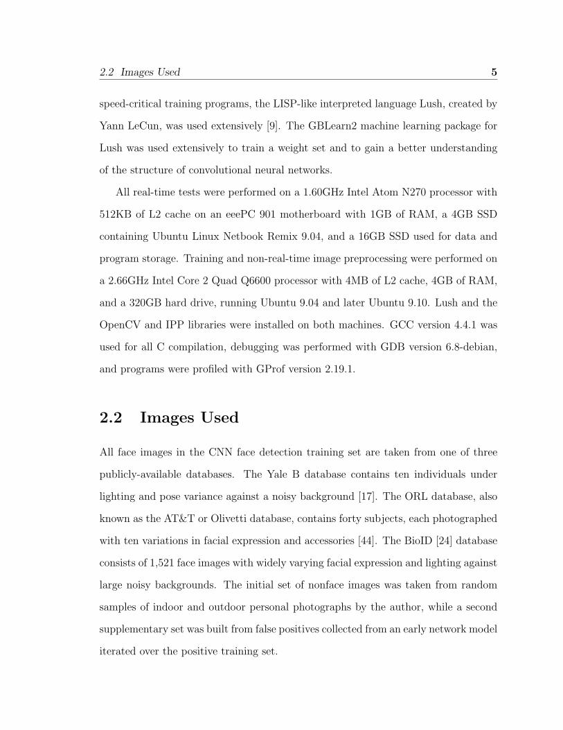
Figure 3.1 The three types of pose variation: (a) side-to-side rotation oryaw, (b) vertical tilt or pitch, and (c) in-plane rotation, or roll
intensive of the two, as it requires applying the same algorithm to each section of an
image at multiple scales. Most techniques produce a single numerical score, confidence
level, or mean squared error value indicating the probability that each given area is a
face, and thresholding is performed to select the final detections. Facial recognition
requires distinguishing each known individual from the others, ideally under variations
in pose (shown in Figure 3.1), lighting, and facial expression, and separating known
individuals from those the system has not previously seen or should not recognize.
Some systems, most notably those based on Eigenfaces or Eigenfeatures, attempt
to detect and recognize faces in a single pass by applying the same method to both
tasks. Recent research has indicated a system designed to simultaneously detect faces
and estimate the pose of each face is more accurate than a system performing either
task on its own [38].

3.1 Facial Recognition Algorithms 11
3.1 Facial Recognition Algorithms
The earliest facial recognition algorithms used the distance between facial features to
identify a unique individual. Some methods computed the apparent absolute distances
between each set of features, while others computed the ratio of distances between
features [50]. These techniques proved to be non-robust in distinguishing individuals
from a large set of known candidates, and were highly susceptible to error due to pose
variation or facial expression. In addition, technologies to find each feature were still
in their infancy, making such approaches unreliable. Almost every facial recognition
technique currently in use can be grouped into one of two categories: algorithms that
treat faces as a collection of related features to be extracted and correlated, and those
that treat the face image as a matrix of intensity values [19].
The most widely used and researched facial recognition techniques are surveyed in
the following sections. Many less-popular methods have been omitted, especially those
that use the additional information dimension of time to find and identify individuals
[57]. By comparing successive frames of a video possibly containing faces, moving
objects on a static background can be more easily segmented simply by finding areas
of change between each frame. Because moving objects may not necessarily be faces,
later methods added shape and color sensitivity to help cull false positives [13]. The
state of the art centers on multimodal methods that take advantage of additional data
available in video for identification, including gait, nonface physical characteristics,
and even audio [7].
3.1.1 PCA and Eigenfaces
One of the most well-known techniques for face recognition and detection, Eigen-
faces, builds upon previous research by Kirby and Sirovich between 1987 and 1990.

3.1 Facial Recognition Algorithms 12
Principal Component Analysis, or PCA, involves discarding the extraneous informa-
tion between correlated sets of variables (in this case, images represented as large
vectors) to greatly reduce the dimensionality of each variable. In pattern recogni-
tion applications, PCA is also known as the Karhunen-Loeve expansion [46]. Kirby
and Sirovich introduced the concept of Eigenpictures, linear combinations of vectors
that could be used to reconstruct image-space pictures; the concept soon evolved
into Eigenfaces [25]. They succeed in creating an arbitrary non-image space between
29 and 210 times smaller than the image space for 128 × 128 face images, achieving
3% reconstruction error using an mutually-orthogonal and orthonormal basis of 40
eigenpictures.
The Eigenfaces technique, developed by Matthew Turk and Alex Pentland, de-
scribes faces as a linear combination of so-called eigenfaces [50]. The algorithm im-
plements a form of PCA that removes the correlation between related numerical
structures, in this case arrays of pixels, to greatly reduce the dimensionality of the
result. Eigenface detection and recognition are related, though recognition requires
one fewer step than detection. In facial recognition using Eigenfaces, as with most
other detection and recognition techniques, a training set must be preprocessed us-
ing a relatively CPU-intensive process to create an emsemble of mutually orthogonal
eigenfaces that defines an Eigenface space. Using a set of sample images of each
known individual, the coordinates of that face in face space can be calculated and
recorded. Detection is performed by mapping an unknown face into face space, then
comparing its coordinates to those of each known individual, usually using a metric
such as the Euclidean distance formula for two N -dimensional face-space vectors a
and b:
d(a, b) =
√√√√N−1∑i=0
(ai − bi)2 (3.1)
The known individual with the smallest Euclidean distance to the candidate image

3.1 Facial Recognition Algorithms 13
is therefore the recognized individual. In systems where unknown individuals may
be seen, a threshold t is applied; if every image pair of candidate c and known face
ki produces a Euclidean distance greater than the threshold such that d(c, ki) > t∀k,
the candidate is classified as an unknown individual [50].
Extracting an Eigenface Space
An Eigenface is the projection of a face image onto a lower-dimensional face space
to make facial recogntion faster and more robust; the approach greatly reduces the
amount of data that must be stored for each face. For example, given a training set
of N training images, each x pixels wide and y pixels high, each known face can be
stored using an order-N vector instead of an order-xy matrix or vector [50]. Given
a training set of M > N faces from which N eigenfaces are to be generated, those
N eigenfaces with the largest associated eigenvalue are retained as the face space
basis. It is meaningless to retain large numbers of eigenfaces; as long as a coherent
set of training images is used for eigenface basis generation, only the first few dozen
eigenfaces are significant [22].
For the sake of simplicity, Eigenfaces are most commonly extracted from greyscale
images of size a× b pixels, such that each image can be represented as an ab-element
matrix of intensity values. Assuming that each input image is square to produce
a = b, each image can be imagined as a vector in a2-dimensional space. If each image
has already been rotated and cropped to contain only an upright face, the first step in
creating an Eigenface space is to transform each a×a image into an a2-length intensity
vector Γi [50]. Normalization may be applied to each intensity vector separately in
some applications, calculated for each jth element of the vector as:
Γi,j =Γi,j
max(Γi)−min(Γi)− min(Γi)
max(Γi)−min(Γi)(3.2)

3.1 Facial Recognition Algorithms 14
Each Γi vector is packed vertiaclly into anM×a2 matrix of intensity vectors. Turk and
Pentland [50] suggest an additional step before packing where the average intensity
vector Ψ is calculated as:
Ψ =1
N
N−1∑i=0
Γi (3.3)
Each row in the intensity matrix is computed as Γi = Ψ− Γi; the authors term this
average-difference matrix the Φ matrix.
Next, the covariance matrix C of the intensity matrix must be calculated by
finding the outer product of Γ:
C = ΓΓT (3.4)
This step transforms the N × a2 matrix of intensity vectors (extended to a2×a2
to meet the square matrix requirements of the outer product) into a symmetrical
a2×a2 covariance matrix. As Turk and Pentland [49] point out, this conceptually-
simple version would be prohibitively resource-intensive, yet would only yield N − 1
eigenvectors with nonzero associated eigenvalues. Therefore, only an N × N matrix
needs to be solved. These authors observe that for all i in [0, N − 1], the eigenvector
i of C is equal to the ith eigenvector of the matrix L = ATA [49]. Therefore, rather
than calculating the covariance matrix C and then extracting its eigenvectors and
eigenvalues, L is constructed as shown, where each element Lmn is defined as:
Lmn = ΦTmΦn (3.5)
Each of the M eigenvectors of L are termed vi. Every eigenface ui is constructed by
summing the dot products of a given eigenvector with each of the Φ vectors. If the
original training set contained M > N faces, the eigenfaces are sorted according to
eigenvalue, largest first, and the first N eigenfaces are retained [50].

3.1 Facial Recognition Algorithms 15
Facial Recognition with Eigenfaces
Once a set of eigenfaces has been created, learning and recognizing faces is compu-
tationally simple. Given a cropped, normalized face image that has been scaled to
the same pixel dimensions as the faces used for training, a vector of N weights ωi is
calculated such that each weight is the dot product of each eigenface with the new
face image minus the average face Ψ:
ωi = ui · (Γ−Ψ) (3.6)
Therefore, to transform any given face from the image space to the face space, a set
of N+1 a2-dimensional vectors are required; namely, the N eigenface vectors and the
average face Ψ [49]. The transformation to face space will yield the set of N weights
that represent the given face; if a candidate face is passed through the same transform,
the Euclidean distance between the weight vector ω of the candidate and the ω for
sample face(s) from the same individual should be smaller than the distances between
the ω of the candidate and those from other individuals. Therefore, by storing a set
of ω vectors for each known individual, any new candidate image can be compared
to all stored weight vectors to determine the identity of the candidate.
3.1.2 Linear Subspaces and Fisherfaces
Eigenface recognition, while effective under controlled lighting and constrained pose,
demonstrates a dramatic decrease in accuracy under variation in head rotation and
illumination. To address this problem, a competing algorithm called Fisherfaces was
developed, also mapping high-dimensional face images to a low-dimensional space via
linear projection. Rather than perform Principal Component Analysis, however, the
algorithm is based around Fisher’s Linear Discriminant (FLD) [6]. The underlying
assumption is that variations in lighting and pose over a single individual changes

3.1 Facial Recognition Algorithms 16
the face image more than the variations between distinct individuals under similar
environmental conditions.
The authors explored an algorithm called Linear Subspaces to improve recognition
performance by calculating a lighting-independent, three-dimensional model of each
face. Faces are described as Lambertian surfaces, defined as surfaces for which appar-
ent lightning of a given point is independent of the observer’s position. Most matte
surfaces are Lambertian, while shiny or mirrored surfaces exhibit non-Lambertian
behavior. Belhumeur et al. [6] define the image intensity E(p) at any point p with
inward-pointing unit normal vector n(p) as:
E(p) = a(p)n(p)T s (3.7)
Here, a(p) is the albedo of the surface, quantitatively representing how much light it
reflects; Lambertian surfaces with lower a(p) values appear darker than those with
higher a(p) values under the same illumination. Since the surface s lies in three-
dimensional space, three images of the same face under the same environmental con-
ditions with three different sets of single-point illumination at known direction vectors
can be used to solve for a(p) and n(p).
Fisherfaces works by using class or individual-specific methods to reduce the di-
mensionality of each image-space image, in contrast to PCA and Eigenfaces, which
apply the same transformation to each input image. Considering each reduced N-
dimension face vector as a point in N-dimensional space, Fisherfaces aims to minimize
the scatter within each class relative to the scatter between points in different classes,
such that images from each class are grouped in distinct clusters. The average of the
images within each ith class Xi is termed µi, Ni is the cardinality of each class Xi,
µ is the overall mean face image, and SB and SW are the inter-class and intra-class

3.1 Facial Recognition Algorithms 17
scatter matrices, respectively:
SB =c∑i=1
Ni(µi − µ)(µi − µ)T (3.8)
SW =c∑i=1
∑xk∈Xi
(xk − µi)(xk − µi)T (3.9)
The ratio SB/SW is to be maximized, so an optimal projection matrix Wopt is cal-
culated. First, a set W of the eigenvectors of SB and SW is computed, sorted in
descending order according to eigenvalue, and pruned to include only the m most
descriptive eigenvectors, a similar process to that used for Eigenfaces. Next, Wopt is
computed to maximize the ratio of interclass scatter over intraclass scatter:
Wopt = arg maxW
W TSBW
W TSWW(3.10)
The authors mention that performing the Fisher Linear Discriminant step first usually
leads to the creation of a singular matrix, so PCA is applied before FLD. The PCA
step is used to reduce the set of N input images covering c classes or individuals to
an (N − c)-dimensional space, then the FLD step reduces it further to a (c − 1)-
dimensional space [56].
Experimental results comparing Eigenfaces, Linear Subspaces, and Fisherfaces
shows the latter to be the most robust when faced with nonuniform lighting [6].
For lighting sources up to 45◦ off the axis normal to the face plane, Fisherfaces
achieves a 4.6% recognition error rate, while a 10-dimensional Eigenfaces implemen-
tation achieves only a 58.5% success rate. Removing the first three eigenvectors from
the 10-dimensional set, suggested by some authors to reduce lighting dependence,
reduces recognition error to 27.7% [6].

3.1 Facial Recognition Algorithms 18
3.1.3 Hidden Markov Models
Several implementations have applied Hidden Markov Models, or HMMs, to the prob-
lem of facial recognition. An HMM consists of a Markov model of finite states with a
probability density function associated with each of its states [36]. HMMs have been
most successfully used for one-dimensional pattern analysis and recognition, such as
signal processing and speech recogntion; facial recogntion has been attempted as a
two-dimensional process [45] and as a one-dimensional segmentation of face features
from top to bottom of a face image [36]. The latter approach achieves an 84% suc-
cess rate on the AT&T face database containing 40 unique individuals. In order to
treat a face image as a 1D signal, the authors utilize the 2D-Direct Cosine Transform
(DCT) algorithm [52] to transform a face image to frequency space, then discard
high-frequency information to simplify recognition. Each image is segmented into
five major features: hair, forehead, eyes, nose, and mouth. For higher recognition ac-
curacy, these features are allowed to overlap. The respective features are then passed
through the HMM, and the closest matching identity is calculated.
3.1.4 Convolutional Neural Networks
Convolutional Neural Networks have been proven to offer a robust solution to image
processing, invariant to moderate geometric transforms such as scale, rotation, trans-
lation, as well as image attributes including brightness and contrast [39] [27]. CNNs
will be explored in detail for the detection of faces in large input images in Section
3.2.5, but have also been applied to facial recognition [26]. Lawrence et al. propose a
system in which a face image preprocessed by Principal Component Analysis is passed
through a CNN containing two convolution layers, two subsampling layers, and one
full-connection layer (arranged in a CSCSF configuration) [26]. A recognition rate

3.1 Facial Recognition Algorithms 19
of 94.25% is achieved on the forty-individual AT&T face database; notably, when
the CNN is replaced with a convention multilayer perceptron neural network (MP),
the error rate increased by a factor of between eight and twelve, depending on other
parameters [26].
3.1.5 Support Vector Machines
Support Vector Machines, or SVMs, offer a conceptually simple method of performing
recognition by segmenting classes in a high-dimensional space [11]. Unlike PCA-based
approaches, which reduce the dimensionality of each point under consideration before
performing any classification, SVMs treat every (m×n)-pixel image as a point in an
mn-dimensional space. Secondly, SVMs compare a candidate point to successive
pairs of known classes to determine its experimental class, rather than comparing the
distances between the candidate and a series of single points in a high-dimensional
space. For a forty-class training set containing ten images of each subject, an SVM
facial recogition implementation achieved an average minimum misclassification rate
of 3.0% [19].
Conceptual Overview
The easiest way to demonstrate SVMs for point classification is to examine a hy-
pothetical set of points, each with two attributes (x, y) such that x, y ∈ R, each
belonging to one of two classes, c0 and c1. Each point can naturally be represented
on a two-dimensional set of axes, as shown in Figure 3.2. SVM training involves
finding the line in this two-dimensional space that optimally divides the two sets.
The optimal separating line will be as far as possible from the nearest points in each
class, and will be chosen to place most, if not all, points of one class on one side
of the line [19]. Since almost every pattern recognition problem to which SVMs are

3.1 Facial Recognition Algorithms 20
f1
f2
d1
d2
Figure 3.2 Simple optimal and suboptimal SVM solutions for two-class sys-tem.
applied involves significantly higher-dimensional points, for example n = 256 dimen-
sions for (16× 16)-pixel images and n = 1024 dimensions for (32× 32)-pixel images,
the boundary becomes a hyperplane in the same n-dimensional space as the data
points.
Mathematical Definition and Derivation
Formally expressed, SVMs solve the problem of separating an arbitrary-sized set
of n-dimensional vectors xi ∈ Rn that each lie in class yi ∈ −1, 1 [11]. The optimal
hyperplane is defined by the points that are the solution of an equation of the following
form, where each wi ∈ Rn is a vector normal to the hyperplane and reaching the
corresponding point xi:
wx− b = 0 (3.11)
The constant b is a scaling factor; since wx = b, the hyperplane is offset by b/‖w‖
from the origin along w. With two linearly separable classes, two parallel hyperplanes

3.1 Facial Recognition Algorithms 21
can be constructed that correspond to b′ = b± 1:
w · x = b+ 1 (3.12)
w · x = b− 1
Stated otherwise, for all points in x, the all points in class yi = 1 should lie on the
far side of the b′ = +1 hyperplane, and all points in class yi = −1 should lie on the
opposite side of the b′ = −1 hyperplane:
w · xi ≥ 1, yi = 1 (3.13)
w · xi ≤ −1, yi = −1
Expressed more succinctly,
yi(w · xi) ≥ 1 (3.14)
It can easily be seen from Eq. 3.14 that the margin between the two hyperplanes
bounding the empty area between the two classes is 2/‖w‖, so Guo et al. [19] define
the optimization problem as minimizing Φ(w) where:
Φ(w) =1
2‖w‖2 (3.15)
Via the dual problem of a Lagrangian functional, the optimal separating hyperplane
is solved in terms of w and b as above in 3.11 as:
w =l∑
i=1
αiyixi (3.16)
b = −1
2w · (xr + xr) (3.17)
The variables r 6= s index αr > 0, αs > 0, where r refers to each point xr in class
yr = 1, and s refers to each point xs where ys = −1. Once w and b have been
calculated, any test point xt can be categorized by:
y = f(xt) = sgn(w · xt + b) (3.18)

3.1 Facial Recognition Algorithms 22
Training sets that are not linearly separable pose a problem for SVMs. In order
to construct a hyperplane separating two such classes with no change to the orig-
inal space, it becomes necessary to introduce some degree of error by minimizing
the number of training points that are misclassified in order to correctly classify a
maximized majority of points. However, a method to properly separate sets that
are initially not linearly-separable has been introduced in the form of kernel func-
tions [11]. The approach circumvents the problem by expressing each of the points in
a higher-dimensional space in which the classes are precisely or nearly linearly separa-
ble, from which w and b can be calculated. However, due to the fact that carrying out
calculations in a space of much higher dimension than the input space may be math-
ematically infeasible, linearly separation in a higher space must be considered in two
separate parts. The first part is the conceptual process using a nonlinear map Φ that
maps from the input space to a higher-dimensional space F , the use of which allows a
linear separation [21]. The second part makes the method implementable on current
computing hardware, the use of a kernel function that eliminates the need to convert
into the high-dimensional space defined by Φ. SVM classification is performed on
linearly-separable points by calculating the dot product of two vectors, for example
w ·xt. If it is necessary to convert to a high-dimensional space before performing the
dot product, then given that w is constructed from Ns support vectors si, Equation
3.18 must be reformulated as [11]:
y = f(xt) = sgn
(Ns∑i=1
αiyiΦ(si) · Φ(x) + b
)(3.19)
The second part of the process is used to replace the computationally intensive
expression Φ(si) · Φ(x) with a cheaper, equivalent kernel function K(si,x), which is
necessary nonlinear [21]. Example kernels include the polynomial K(x,y) = (x · y)d
and the tan-sigmoid with constants κ and Θ expressed as K(x,y) = tanh(κ(x·y)+Θ).

3.2 Facial Detection Techniques 23
SVMs for Facial Recognition
Since SVMs can only distinguish between two classes at a time, it is necessarily to
iteratively eliminate possible categories for a given test point to leave a single matching
category [19]. Given c categories, it must be possible to determine whether a point
falls into category ci or cj, i 6= j, i, j ∈ [1, c]. This defines C = c(c − 1)/2 possible
comparisons, so a set of C w and b values must be trained. One possible facial
recognition implementation performs a bottom-up binary tree search to determine
the identify of a given face by first performing C/2s comparisons on successive stages
s = 1, 2, ..., log2(C) until a single class remains.
3.2 Facial Detection Techniques
Face detection, also termed segmentation or localization, covers the task of finding
zero or more faces against a possibly arbitrary background. Depending on the appli-
cation, most detectors should also be able to find faces with variation in pose (roll,
pitch, and yaw), lighting, and scale [22]. Some detectors are even designed to find
occluded or partially-obscured faces. In general, the most popular segmentation tech-
niques are divided into two categories. The first is based on searching for whole faces
within an image, while the second searches for individual features like eyes, noses,
mouths, and ears, then attempts to find faces based on proximity of coherent features
in face-like configurations. Each method has been approached many difference ways,
though most involve some training to extract relevant information from known faces
and non-faces before testing can be performed. Hjelmas and Low [22] identify three
areas of feature-based face detection:
1. ”Low-level” analysis that looks at edges, colors, movement, and even symmetry
rather than searching for specific shapes and patterns.

3.2 Facial Detection Techniques 24
2. Higher-level searches for discrete features, especially eyes, noses, and mouths.
3. ”Active shape” models that track the structure of the face to determine feature
locations.
The authors also address three types of full-face face detection techniques, all of which
are addressed in some form in this section:
1. Methods to reduce the dimensionality of the face space, such as PCA and Eigen-
faces.
2. Neural networks, including multilayer perceptrons (MPs) and convolutional
neural networks (CNNs).
3. Stochastic or probabalistic approaches that use SVMs or Bayesian decision the-
ory.
Besides the methodologies explored in depth in the following sections, many fa-
cial and pattern recognition techniques have been applied to the problem of facial
detection, with varying success. Support Vector Machines were used to perform fa-
cial detection, yielding competitive detection rates at higher speeds than previous
systems [40]. The K-Nearest Neighbor (KNN) algorithm is one of the conceptually
most straightforward pattern-matching and classification algorithms, but historically
considered one of the least effective against possible translation, rotation, and image
characteristics such as brightness and constrast. Very early face detectors were im-
plemented with such algorithms, but the most recent uses have been for verification
or correlation within other more complex systems, or for face-related tasks such as
expression recognition [41].

3.2 Facial Detection Techniques 25
3.2.1 Eigenfaces
Facial detection using the Eigenface method is conceptually simple and relatively
fast, but is more susceptible to inaccuracy from pose, lighting, and scale than other
methods. To determine whether a given image sample is a face or not, assuming
that the candidate image has the same pixel dimensions as the training faces used
to construct the eigenfaces (and therefore that its intensity vector’s length is equal
to the length of each eigenface vector), the image must be converted to face space,
then back to image space. The conversion to face space is performed just as for face
recognition:
ωi = ui · (Γ−Ψ) (3.20)
Once the vector ω = (ω0, ω1, · · ·ωN−1) has been calculated, it is used to reconstruct
the input image in image space:
Γ′ =N−1∑i=0
ωi · ui (3.21)
The standard Euclidean distance algorithm as specified in Equation 3.1 is used to de-
termine the difference between the input image and the reconstructed image; since by
definition an Eigenface system encodes a basis of images discarding the commonalities
between different face images, such a reconstructed image will necessarily resemble a
face, albeit one not corresponding to any particular individual. For nonface inputs,
the difference between this reconstruction and the original should be larger in mag-
nitude than between a face image and its reconstruction, even with some lighting
variance, shift, rotation, or scaling. A threshold t can be set such that every sample
or subimage with a difference ‖Γ′ − Γ‖ ≤ t is taken to be a face, but even subimage
with ‖Γ′ − Γ‖ > t is not a face. As with most other facial detection algorithms,
a second technique can be used in parallel or serial with Eigenfaces to reject false
positives, catch missed detections, or both.

3.2 Facial Detection Techniques 26
3.2.2 Eigenfeatures
Eigenfeatures are very similar to eigenfaces, and work on exactly the same mathe-
matical prinicipals. A set of known features, such as eyes and mouths, are used to
construct eigenfeatures including “eigeneyes” and “eigenmouths” [35], grouped into a
category called eigentemplates that are more robust at localizing features than previ-
ous template-matching methods. The same technique is used to search for features in
large input images as faces: each area of the image is converted to the feature space
and back to the image space at multiple scales, and those areas for which the mean
squared error is below a certain threshold are judged to contain the desired facial
features. The most efficient systems in this category search for a single facial feature
such as a mouth first, then intelligently search the area above each possible mouth
for a nose and eyes. If all or some of the constituent features of a face are found, the
area is a face. This may be the endpoint of the process, or the extracted face may be
passed to a normalization and/or recognition algorithm.
3.2.3 Haar Classifier
The Haar classification method, designed by Viola and Jones, attempts to reduce
the computational cost associated with analyzing large arrays of pixels and multiple
scales by dealing instead with contrast-delineated features [55]. These features do not
correspond to objects such as eyes and ears, but rather to classes such as relatively
light areas next to relatively dark areas, dark areas surrounded by lighter areas, and
lengths of lighter color bounded on two sides by dark areas. Conceptual samples of
Haar features as defined by pixel intensities are shown in Figure 3.3 [12].
Conversion from image space to Haar feature space is performed in two steps.
First, the raw image is transformed into an integral image with the same dimensions

3.2 Facial Detection Techniques 27
Figure 3.3 Simplified Haar features, including edges (top row), dark andlight lines (middle row), and surround features and line termini (bottom row).Real Haar features are generally larger than 3× 3 pixels, more complex, andconsist of fractional shades between light and dark.
as the original image, in which the values of each element are the sums of all pixels
above and to the left of that element [55]. Formally expressed, for input image A and
integral image I with equal pixel dimensions, the value of any element of the integral
image Ix,y is:
Ix,y =x∑
m=0
y∑n=0
Am,n (3.22)
The integral image is created so that the sum of the pixels within any given rectangle
can be found with a simple sum of six to eight values from the integral image regardless
of the size of the rectangle [55]. In addition, many implementations also rotate the
original image by 45◦ and calculate a second integral image from this rotated original
so that tilted features can also be considered, such as diagonal lines or edges.
Once integral images have been created, the second stage of the detector is a
cascaded classifier. Although each desired object, for example a face, consists of a
combination of many Haar features, subimages that do not contain the desired object
can be discarded by searching for only a small subset of this total feature description.
By searching the entire image at multiple scales for only a few features, a portion of
the input can be discarded, leaving a smaller total area to be searched using more
features. At the end of the process, only the subimages containing positive detections

3.2 Facial Detection Techniques 28
using all of the descriptive features will be retained. The advantage of this cascaded
system is that the calculations for the full Haar feature set do not have to be completed
at every possible subimage, leading to a significant savings in computation time even
with the overhead of maintaining an enumeration of which areas have or have not been
discarded. A system using the Haar classifier for multiscale face detection achieved a
rate of 5 frames per second with 95% accuracy [55].
3.2.4 Neural Networks and Multilayer Perceptrons
Traditional neural networks or multilayer perceptrons, supposedly built with a struc-
ture similar to that of biological vision processors such as the human brain, have been
considered as candidates to perform facial detection and to a more limited extent,
facial recognition. As with most algorithms that detect faces in a larger image at
multiple scales, the proposed systems extract all possible subimages that could con-
tain a face, use each as the input to one or more linearly- or nonlinearly-connected
neural networks, and interpret the output as a binary value indicating the presence
or absence of a face [43]. The weights of the neural networks are trained using classic
backpropagation [16]. However, these detectors are poor candidates for a real-time
face detection system, as a full set of values must be propagated through the network
for every window, including neighbors that share the majority of their pixels through
overlap. One implementation required 383 seconds to process a 320x240 pixel image
with two complementary neural networks on a 200MHz machine [43], and 7.9 sec-
onds with compromises made to accelerate the process; the authors report between
77.9% and 90.3% accuracy. A second implementation processes roughly 1 frame per
second on a 333MHz computer examining similarly-sized images with five parallel
networks [16].

3.2 Facial Detection Techniques 29
… … … …
Input LayerHidden Layer Hidden Layer
Output Layer
Figure 3.4 Standard neural network architecture. In a multilayer percep-tron, nonlinear activation functions are used to connect neurons.
Neural Network Structure
The canonical structure of a neural network with two hidden layers is shown in Figure
3.4. This example contains a one-dimensional input layer, two larger hidden layers,
and a smaller one-dimensional output layer. In this standard configuration, each layer
is fully connected to its neightboring layers, such that between two sequential layers
ln and ln+1, containing Nn and Nn+1 neurons respectively, there exist Cn = Nn ·Nn+1
connections. Typically, no form of weight-sharing is used, therefore the number of
weights necessary to describe a network is equal to at least the number of connections
in that network, often close to twice the number of connections considering weights
and biases. The activation functions, or mathematical relationships between the
output of a neuron and its input, may be either a linear or nonlinear function. Linear
functions for the output of the jth neuron of the nth layer are generally in the following
form, where each neuron has an associated bias bn,j and a set of input weights wn,i,j
such that the output is a weighted sum of the inputs plus a bias [32]:
an,j = bn,j +
Nn−1−1∑i=0
wn,i,j · an−1,i (3.23)

3.2 Facial Detection Techniques 30
Nonlinear neurons can similarly be described by passing the weighted sum of input
neurons into an activation function f . In some cases, the bias bn,j is omitted.
an,j = f
(bn,j +
Nn−1−1∑i=0
wn,i,j · an−1,i
)(3.24)
This discussion generalizes to a fully-connected structure for the sake of simpli-
fied notation. Networks that are not fully-connected operate similarly. Nonlinear
activation functions generally follow the form of a sigmoid function, also known as a
squashing function [20]. One specific sigmoid constructed using the hyperbolic tan-
gent function, called the tan-sigmoid in contrast to the log-sigmoid, is discussed in
more detail in Section 3.2.5. The class of sigmoid functions act like a smooth step
function, limiting the output of a neuron to positive or negative asymptotes for large-
magnitude inputs, but producing a roughly linear output for inputs close to zero. A
neuron is said to be saturated if its ouput is near one of the asymptotes of its sigmoid.
Sigmoids are used for the activation functions of multilayer perceptrons (MPs).
Neural Network Training
Most multilayer perceptrons, as well as Convolutional Neural Networks as described
below, are trained using some variation of backpropagation and gradient descent.
The weights of the network are initialized, usually to values generated from a chosen
random distribution [27,28,43], and an iterative training process is carried out on some
set of training data. Data is expressed as a set of ordered pairs of input and output
vectors so that the backpropagation method can be used to modify the weights of the
network based on the differences between the actual output and the expected output.
For the single output layer with layer index n, each of the Nn output nodes with
forward-propagated values an,j=oj differs from the expected output vector t by the
simple difference δj = tj−oj. These error values can only be backpropagated through

3.2 Facial Detection Techniques 31
the network for differentiable activation functions; for example, the derivative f ′ of
the tan-sigmoid is 1− f 2. The error for each hidden layer is more complex, and must
be solved using a gradient-based method: each hidden layer n is examined, starting
from the ouput layer and working backwards towards the input layer. For the output
layer n containing Nn neurons, the total error E is the standard sum-squared error
function:
E =1
2
Nn∑j=0
(tj − oj)2 (3.25)
The contribution of each output node to the total error can be easily calculated with
a gradient, yielding the expected result, such that the output function f is used as in
Equation 3.24.
δj =∂E
∂oj= 2 · 1
2· (tj − oj) · −f ′(oj) = −(tj − oj)f ′(oj) (3.26)
For a linear activation function, f is the identity function f(oj) = oj, f′(oj) = 1, and
δj = −(tj − oj).
Of principle importance in training the weights of the network is the error in each
weight wn,i,j for neuron n, j, or ∂E∂wn,i,j
. Since the output of every node is a weighted
sum of activation functions, the contribution of each of the inputs an−1,i is∂an,j
∂wn,i,j, so
the following substitution can be made:
∂E
∂wn,i,j=
∂E
∂an,j· ∂an,j∂wn,i,j
=∂E
∂an,j· an−1,i = δn,jan−1,i (3.27)
It is important that the network not be trained to fit perfectly to a given training
example on every iteration, as a network thus trained would never converge to a
globally acceptable minimum error. To prevent this, a learning rate η is introduced,
generally on the order of 10−1 to 10−3, that is used as a coefficient to all weight
updates. The error in a given weight must be reduced by adding the negative value
of its error, so from Equation 3.27, the change made to any given weight wn,i,j during
3.2 Facial Detection Techniques 32
a backpropagation iteration will be [20]:
∆wn,i,j = −η ∂E
∂an,j· an−1,i = −ηδn,jan−1,i (3.28)
The final component necessary to complete the algorithm is to define the δn,j
values for all non-output neurons in the network. It is still necessary to calculate
∂E∂wn,i,j
; in order to determine this value, the set of every neuron downstream (closer
to the output) that is connected to the current neuron delineates the complete set
of δn+1,k∀k ∈ [0, Nn+1 − 1] values that contribute to the current neuron’s δn,j. Con-
sidered in reverse, the error accumulated in the current neuron in layer n can only
directly affect those neurons in layer n+ 1 that are directly connected to this neuron,
and indirectly all neurons downstream of those neurons. The expression [20] for the
gradient of the error with respect to each input weight wn,i,j of the jth neuron in
layer n, where the output of a neuron an,j = f(zn,j), is:
δE
∂wn,i,j=
Nn+1−1∑k=0
∂E
∂zn+1,k
· ∂zn+1,k
∂an,j· ∂an,jδzn,j
· ∂zn,j∂wn,i,j
(3.29)
As in the rest of this discussion, a fully-connected network is assumed; if the given
network is not fully-connected, or if neurons are connected to those in other layers
other than that directly above them, then the bounds of the summation in Equation
3.29 can be expressed as k ∈ downstream(n, j). Simplification of backpropagation is
possible based on the equations above; ∂E∂zn+1,k
is simply δn+1,k, and the ratio of any
neuron’s output to its weighted sum∂an,j
δzn,jis the derivative of its activation function
f ′(an,j). The ratio of a weighted sum to one of its inputs reduces to the associated
weight, or∂zn+1,k
∂an,j= wn+1,j,k, and similarly,
∂zn,j
∂wn,i,j= an−1,i. This allows Equation 3.29
to be restated as:
δE
∂wn,i,j=
Nn+1−1∑k=0
δn+1,k · wn+1,j,k · f ′(an,j) · an−1,i (3.30)

3.2 Facial Detection Techniques 33
Only the final term, an−1,i, is dependent on specifying the ith input from the (n−1)th
layer, so to derive the per-neuron error δn,j, an expression for δE∂zn,j
is required [28]:
δn,j =δE
∂zn,j=
Nn+1−1∑k=0
δn+1,k · wn+1,j,k · f ′(an,j) (3.31)
A final simplification can be performed by moving the k-independent f ′ term outside
the summation, yielding the final expression for the error of any hidden neuron with
output an,j:
δn,j = f ′(an,j)
Nn+1−1∑k=0
δn+1,k · wn+1,j,k (3.32)
As previously stated, this error expression from Equation 3.32 can be used in Equation
3.28 to calculate the change in each weight.
After working backwards through the entire multilayer perceptron and updating
all weights as necessary, a new training sample can be forward-propagated through
the network and the process is repeated. Iterating through the full set of samples in
the training set is known as a epoch in neural network terminology. Fully training a
given neural network usually takes a very large number of epochs; training is judged as
complete when some criterion is fulfilled, such as convergence of the weights to within
some arbitrary value. Although not used directly for this project, backpropagation for
multilayer perceptrons is the foundation to understand the backpropagation algorithm
for convolutional neural networks, detailed in Section 3.2.5.
3.2.5 Convolutional Neural Networks
Rather than using a set of templates to match faces or features, convolutional neural
networks (CNNs) have recently been successful for detecting faces in large images.
Classical neural networks, or multilayer perceptrons, had been previously applied
to the problem with limited success; the properties of CNNs make this approach

3.2 Facial Detection Techniques 34
better-suited to realtime detection of faces in large images than MPs. Such networks
have been proven robust under variation in shift, deformation [26], scale, lighting,
occlusion, facial expression, skin color, and accessories [39]. Notable applications of
CNNs include optical character recognition [27], object classification under extreme
rotation variance and class diversity [29], and facial detection [51] [26] [38] [39].
CNN Components
Any convolutional neural network consists of a series of layers, where each layer
performs either convolution, subsampling, or full connection. A convolutional (C)
layer acts as a feature extractor, such that one or more outputs from the previous layer
are convolved with one or more fixed-size kernels to produce its output or outputs,
as shown in Figure 3.6. A subsampling layer (S) contributes to CNNs’ robustness to
scaling, rotation, and offset; the substructure of the subsampling operation is shown
in Figure 3.7. A full-connection layer (F), explained in Figure 3.8, performs a set
of dot products to compute the outputs of the neural network. The CNN model
is based on a combination of previous research with linear multilayer perceptrons
and research into the neural mechanisms of vision processing in human and animal
brains [27]. Current CNN architectures have been designed through trial-and-error;
larger networks with more layers are generally more accurate given a fixed number of
categories or output nodes, and larger networks are necessary to maintain accuracy
given more categories.
Each convolutional layer of a neural network takes one (m× n)-pixel layer as an
input, performs convolution with N k×k kernels, adds one of N scalar bias values, and
outputs N layers, each of size (m−k+1)× (n−k+1). The function of the layer is to
perform feature detection on a set of N specific features; by scanning across the entire
input layer, some degree of shift invariance is introduced. In addition, by convolving

3.2 Facial Detection Techniques 35
Subsample
Convolution
Input32x32
C16@28x28
S26@14x14
C316@10x10
S416@5x5
C5120
F66
Convolution Subsample
Convolution
Full Connection
Figure 3.5 Lenet-5 CNN Architecture
with the same kernel across the input layer to produce each of the N outputs, CNNs
introduce weight-sharing that allows for a more complex neural network structure
without exponentially increasing the number of neuron weights and offsets that must
be trained. For example, the standard Lenet-5 implementation shown in Figure
3.5 utilizes a set of 60,000 weights shared between 340,908 connections. The first
convolutional layer, C1, contains only 156 trainable parameters in six 5×5 kernels plus
six bias values to produce 122,304 total connections [27]. In the second convolutional
layer, alternately termed C2 for being the second convolutional layer or C3 to indicate
the presence of the intermediate subsampling layer, 1, 516 weights are shared between
151, 600 connections. The third and final convolutional layer, heretofore termed C5,
uses each of the 48,120 weights once. In CNN terminology, the 1 × 1 output unit
to which each 5 × 5 input area maps is called the receptive field for that input;
neighboring receptive fields share most of their inputs, ensuring that a feature will be
detected regardless of where in the input layer it falls. Notably, the features that will
be selected by a CNN during its training do not necessarily correspond to features
that a human might select as significant.
The C3 layer, or permutating convolutional layer, constructs each of its outputs
from a selection of S2 outputs, according to the order shown in Table 3.1. This con-
nection configuration performs a primary duty of maximizing the number of different

3.2 Facial Detection Techniques 36
features extracted by the C3 layer, since each convolution sees a different set of input
layers, and also helps to lower the number of weights to be trained for the C3 layer
by about 38%. Six of the C3 outputs are constructed from combinations of three S2
outputs, nine from combinations of four S2 outputs, and one from all six S2 outputs.
The convolution and subsampling performed by the C1 and S2 layers ensures that
some degree of feature accentuation and spatial-dependency reduction has already
been performed, increasing the robustness of the C3 feature detector.
C3 Output Units0 1 2 3 4 5 6 7 8 9 10 11 12 13 14 15
C3
Input
Unit
s 0 × × × × × × × × × ×1 × × × × × × × × × ×2 × × × × × × × × × ×3 × × × × × × × × × ×4 × × × × × × × × × ×5 × × × × × × × × × ×
Table 3.1 Permutation connections from C3 inputs to C3 outputs in Lenet-5
The third and last convolution layer, C5, convolves each of the 16 outputs of the
S4 layer, each 5× 5, with a set of 120 equally-sized kernel, adds a bias, and produces
a 120-element vector. As noted by the creators of Lenet-5 [27], this layer essentially
a full-connection layer, but describing it as a convolution allows more flexibility for
larger network versions for which the C5 inputs are larger than 5x5. F6 is a true
full-connection layer with p outputs, multiplying each element of the C5 output by p
different weights and adding p biases; the C5 to F6 connection is the section of the
Lenet-5 CNN that is most similar to a classical multilayer perceptron in form and
function.
The subsampling layers of a convolutional neural network add robustness against
spatial-dependence while reducing the number of weights and computation necessary
for the sections of the CNN following that subsampling layer. While a subsampling

3.2 Facial Detection Techniques 37
Figure 3.6 CNN Convolutional Layer StructureEach element of the output is constructed from a convolution of an area of theinput matrix with a fixed-size kernel; the same kernel is used to generate theentire output matrix. Neighboring output cells share input cells to minimizemissed feature detection.
layer can be implemented with any step size greater than 1, and can use a different
step along the x and y axes, the most common implementations use a step size
of 2 on both axes, such that the dimensions of the outputs of the layer are half
that of the inputs, and each output contains one-quarter the number of pixels as
the input. Given stepping on the respective x and y axes xstep and ystep, each 1x1
output of the subsampling layer is the average of the associated xstep × ystep area of
the input, such that a feature detected anywhere within that xstep × ystep rectangle
will be equally detected at the output of the subsampling layer. An interleaved
architecture of convolution and subsampling layers provides robust shift invariance
without compromising the accuracy of the convolutional feature extractors.
Because of the multiplicative and additive nature of the CNN, it would be un-
desirable for layer outputs to increase outside of certain bounds, as increases could
propagate into larger and larger values in a complex network. To this end, a sigmoid
is applied to the output of each convolutional, subsampling, and full-connection layer.
The sigmoid function used is close to linear on the domain [−1, 1], becoming increas-

3.2 Facial Detection Techniques 38
Figure 3.7 CNN Subsampling Layer StructureEach cell in the output matrix is the average of a larger set of cells in theinput matrix. Unlike the convolutional layer, no two output cells share anyinput cells.
ingly flat for values with magnitudes above unity, and approaching an asymptote of
±1.7159 at ±∞; it is defined as f(x) for some input x as:
f(x) = 1.7159tanh
(2
3x
)(3.33)
Therefore, every layer except C1 is designed to accept input within the range [-
1.7159 1.7159], and the final outputs of the CNN will all fall within the same range.
Because the sigmoid function most closely approximates the linear function f(x) = x
at x = ±1, CNNs identifying discrete object classes usually use 1 to represent a
positive result from the F6 layer, and −1 to represent a negative result.
A full connection layer can have as many or as few elements as the application
requires. A CNN generally has a single full connection layer as the last stage of the
network, although additional such layers could used anywhere in the network if re-
quired by the application. The simplest form of a CNN would indicate the binary
presence or absense of an object within the input by a single scalar output, such
that values close to −1 indicate the object’s absence, and values close to 1 indicate

3.2 Facial Detection Techniques 39
Figure 3.8 CNN Full Connection Layer StructureThe element of the output vector (bottom) is a dot product of the inputvector (top) with a kernel vector of the same dimensions as the input vector.
its presence. The smaller the Euclidean distance between the output value and the
decided target value (±1), the higher the confidence of the positive or negative detec-
tion. It has been found that CNNs produce more accurate results for single-category
detection when there is a second class c1 indicating the absence of the target object,
such that for most input images c1 ≈ −c0 [27]. For more classes of object, additional
dimensions can be added to the output of the network’s full connection layer, but for
more than roughly thirty or forty classes, performance degrades significantly when
each output neuron indicates the presence of one object type [27]. It becomes diffi-
cult for the network to keep all of the outputs near −1 for almost all inputs, and 1
only for the rare cases when the input image includes that object. Several possible
solutions are suggested depending on the requirements of the application; previous
approaches include arranging the outputs in a 2D matrix with stylized bitmap im-
ages of each letter used to calculate the optimal activation pattern for each character
in the ASCII set [27] and designing a function to represent the yaw and roll of the
objects detected by the values of the outputs in a network that estimates object ori-
entation [39]. Therefore, categories in a CNN are not mutually exclusive, and any
image can be classed into any combination of classes or parameter values, depending
on the intended interpretation of the output values.
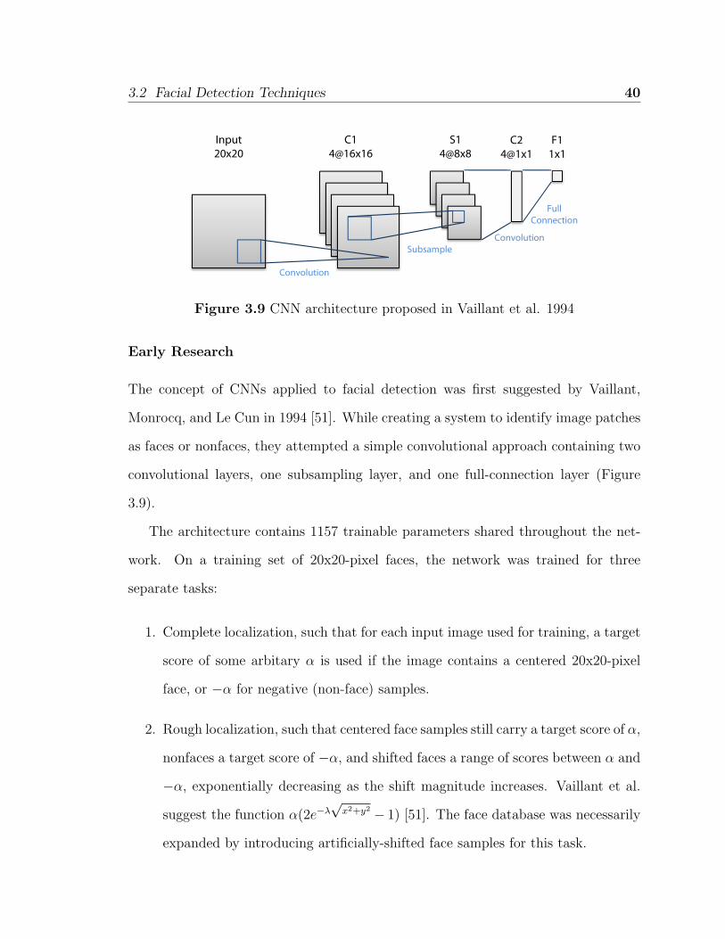
3.2 Facial Detection Techniques 40
Convolution
Full Connection
Subsample
Convolution
Input20x20
C14@16x16
S14@8x8
C24@1x1
F11x1
Figure 3.9 CNN architecture proposed in Vaillant et al. 1994
Early Research
The concept of CNNs applied to facial detection was first suggested by Vaillant,
Monrocq, and Le Cun in 1994 [51]. While creating a system to identify image patches
as faces or nonfaces, they attempted a simple convolutional approach containing two
convolutional layers, one subsampling layer, and one full-connection layer (Figure
3.9).
The architecture contains 1157 trainable parameters shared throughout the net-
work. On a training set of 20x20-pixel faces, the network was trained for three
separate tasks:
1. Complete localization, such that for each input image used for training, a target
score of some arbitary α is used if the image contains a centered 20x20-pixel
face, or −α for negative (non-face) samples.
2. Rough localization, such that centered face samples still carry a target score of α,
nonfaces a target score of −α, and shifted faces a range of scores between α and
−α, exponentially decreasing as the shift magnitude increases. Vaillant et al.
suggest the function α(2e−λ√x2+y2 − 1) [51]. The face database was necessarily
expanded by introducing artificially-shifted face samples for this task.

3.2 Facial Detection Techniques 41
3. Precise localization, using the same set of images as for rough localization, but
with shifted faces carrying a score of −α.
Qualitatively, the network trained for rough localization was the most successful,
producing a blob of detections within the area of each face in a given (256 × 256)-
pixel test image. The authors suggest that postprocessing could be used to eliminate
isolation detections while retaining grouped detections. The two networks trained for
complete localization and precise localization respectively produce unusable results;
although each network produces a false classification rate (combined missed detection
and false positive rates) of about 4%, no coherent result can be obtained.
CNNs for Facial Recognition
As discussed in Section 3.1.4, CNNs have been used as part of a facial recognition
system as well as for facial detection. However, used independently CNNs produce
subpar recognition rates. [26] A CNN contains subsampling layers interleaved with
feature detectors in order to reduce location sensitivity, performing object recognition
based on the configuration of features rather than the exact intrafeature distances.
A face recognizer should ideally perform the opposite task, keeping the intra-feature
distances as equally significant to their spatial distribution. As demonstrated by
applying CNNs to the task of non-face object classification [29], CNNs are best suited
to binning objects into classes even with wide shape variance between members, a
capability that reduces their effectiveness for the task of facial recognition.
Lenet-5 and Facial Detection
The architecture of the Lenet-5 CNN is described as an example earlier in this sec-
tion; it consists of six layers in a CSCSCF arrangement, where each C layer uses 5x5
kernels, the input to the network is 32x32-pixel grayscale images, all subsampling
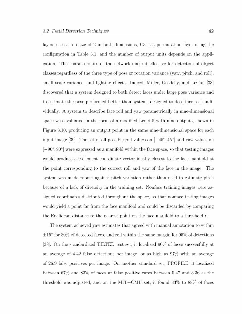
3.2 Facial Detection Techniques 42
layers use a step size of 2 in both dimensions, C3 is a permutation layer using the
configuration in Table 3.1, and the number of output units depends on the appli-
cation. The characteristics of the network make it effective for detection of object
classes regardless of the three type of pose or rotation variance (yaw, pitch, and roll),
small scale variance, and lighting effects. Indeed, Miller, Osadchy, and LeCun [33]
discovered that a system designed to both detect faces under large pose variance and
to estimate the pose performed better than systems designed to do either task indi-
vidually. A system to describe face roll and yaw parametrically in nine-dimensional
space was evaluated in the form of a modified Lenet-5 with nine outputs, shown in
Figure 3.10, producing an output point in the same nine-dimensional space for each
input image [39]. The set of all possible roll values on [−45◦, 45◦] and yaw values on
[−90◦, 90◦] were expressed as a manifold within the face space, so that testing images
would produce a 9-element coordinate vector ideally closest to the face manifold at
the point corresponding to the correct roll and yaw of the face in the image. The
system was made robust against pitch variation rather than used to estimate pitch
because of a lack of diversity in the training set. Nonface training images were as-
signed coordinates distributed throughout the space, so that nonface testing images
would yield a point far from the face manifold and could be discarded by comparing
the Euclidean distance to the nearest point on the face manifold to a threshold t.
The system achieved yaw estimates that agreed with manual annotation to within
±15◦ for 80% of detected faces, and roll within the same margin for 95% of detections
[38]. On the standardized TILTED test set, it localized 90% of faces successfully at
an average of 4.42 false detections per image, or as high as 97% with an average
of 26.9 false positives per image. On another standard set, PROFILE, it localized
between 67% and 83% of faces at false positive rates between 0.47 and 3.36 as the
threshold was adjusted, and on the MIT+CMU set, it found 83% to 88% of faces

3.2 Facial Detection Techniques 43
Subsample
Convolution
Input32x32
C18@28x28
S28@14x14
C320@10x10
S420@5x5
C5120
F610
Convolution
Subsample
Convolution
Full Connection
Figure 3.10 CNN architecture proposed in Osadchy et al. 2007
with an average of 0.50 to 1.28 false positives per image.
Training a CNN
Although the structure of a Convolutional Neural Network is superficially much more
complex than a canonical Multilayer Perceptron, a CNN still contains hidden neu-
rons at each layer whose outputs are the weighted sums of inputs passed through
a nonlinear activation function, in this case the differentiable tan-sigmoid equation
passing the origin shown in Equation 3.33. All three layer types add a trainable scalar
bias to a sum of weighted products before appplying a sigmoid, so backpropagation
can be applied to each as described in Section 3.2.4 [27]. The convolution (C) and
subsampling (S) layers are not fully connected, making the notation to describe the
relationship between the inputs and outputs of each layer’s neuron more complex, but
reducing the number of inputs that contribute to each output. The full connection
(F) layer operates identically to a hidden layer in a standard multilayer perceptron.

3.3 Wearable Computing and Augmented Reality 44
3.3 Wearable Computing and Augmented Reality
As digital information has become an integral part of daily life, various methods have
become popular to access this data and interact with it. Mobile telecommunications
devices are ubiquitous, providing voice communication and limited data capabilities.
Laptops, PDAs, and smartphones are light and powerful enough to take anywhere
and handle most basic information storage and retrieval tasks. However, technology
to directly combine the real world with digital information remains in its infancy.
With so much important information available in the virtual world, it has become
important to efficiently access and interact with this information throughout daily
life; augmented reality (AR) offers a solution [31].
An augmented reality system is defined as one which overlays or augments virtual
or digital information over the real world [15]. This may take the form of a handheld
device with a camera and a display, a wearable computing system with a camera and
a head-mounted display, or any of a number of computing devices coupled with input
and/or output hardware. Augmented reality itself is the process of supplementing the
real world with additional data, in contrast to augmented virtuality, which modifies
a virtual environment with information, text, video, or audio from the real world
[15]. At the far ends of the real-virtual spectrum, or Milgram’s Continuum [8], are
telepresence systems that show simple, unaugmented video, and virtuality systems
that synthesize, display, and allow exploration of artificial universes.
Within augmented reality systems, further subdivisions exist with regard to what
type of information overlay is performed, depending on the needs of the application.
The simplest type provides contextual information such as text, images, or audio,
displayed in a position selected to be unobtrusive rather than to correspond to some
specific feature in the physical environment. Examples include messages received from

3.3 Wearable Computing and Augmented Reality 45
a text- or instant-messaging source, general environmental information, or location-
specific notes. A more complex overlay annotates specific objects in a scene, usually
by detecting or localizing pre-existing physical objects within the environment or by
reading specialized tags such as 2D barcodes [47, 53]. The most advanced systems
use contextual image processing techniques to find specific objects [30] or surfaces
within a scene, determine their orientation and apparent size, and modify them with
additional virtual objects. For example, virtual objects can be placed on a physical
tabletop, or with the addition of gesture recognition, a fully-virtual touchscreen could
be created on a real-world wall [31].
3.3.1 Hardware
While prototypical AR systems are feasible on standard commodity computers for the
sake of rapid development, real-world testing of most such applications requires a more
portable system. The computational unit used to interpret visual, audio, or location-
based information must be small and light enough to be transported by the user with
ease. Input and output is normally not performed with a standard keyboard, mouse,
and fixed monitor; in most cases the wearable AR system is acting as a secondary
input while the user performs other primary tasks. All hardware must be unobtrusive
and socially acceptable to be feasible for use in daily life [53], a set of criteria that
most available heads-up displays do not meet. Onboard batteries should ideally be
sufficient for a full day of computing without charging, making the function of the
system as transparent to the user as possible. Necessary communications capabilities
vary depending on the application, but may include an IEEE 802.11 WiFi module or
a cellular telephone connection [53].

3.3 Wearable Computing and Augmented Reality 46
Computing Hardware
Wearable computing occupies a challenging engineering niche at the intersection of
high performance, lightweight, portable design, and long battery life. Many solutions
have been proposed and tested, including unmodified commodity laptops and per-
sonal organizers, modified commodity systems, and custom-built prototypes. A wide
variety of capabilities has been explored, depending on the particular application. As
noted in Section 3.3.1, solutions to mitigate the limitations of portable, low-resource
hardware have centered on the use of a tethered or wireless connection to a more
powerful fixed server running image processing or other application-specific software.
A project to localize and recognize two-dimensional barcodes in an environment used
the commodity HP iPaq portable digital assistant (PDA), built around a 400MHz
XScale processor with no Floating Point Unit (FPU) and limited RAM and storage
capacity [53]. Indeed, some augmented reality projects intended for use in one fixed
location have directly taken advantage of the power of commodity desktop or server
computers [31], and others ignored portability problems in the interest of developing
a robust localization or recognition system before constraining it to portable sys-
tem [30,54]. An intermediate solution used in several projects employs a “backpack”
containing a commodity laptop, battery, and interfacing hardware as an augmented
reality platform [8]. Another solution used a single-board computer containing RAM,
a processor, and storage to which additional modules can be added [47].
Shared Processing
The portability constraints on wearable computing system necessarily limit the amount
of processing power available. The lighter the device used to process environmental
and secondary input and produce meaningful output, the fewer capabilities the ma-
chine must have. In addition, space-consuming components, such as large batteries

3.3 Wearable Computing and Augmented Reality 47
and an extensive variety of ports and connectivity options, are impossible to fit in a
light-weight wearable computer. To bring arbitrary speed and capabilities to wear-
able computing systems, offloading of computational load over wireless networks has
been proposed [53], which may be implemented as one of several different architec-
tures based on the needs of the application. Each possible design shares processing
load between the local, low-capability wearable client and a more powerful remote
server. The typical AR system examines frames from a head-mounted camera, per-
forms some image-processing steps, passes the results through an application-specific
algorithm to extract or provide meaningful information from the image-processing
output, renders the augmented overlay, and displays it with the original image. A
fully self-contained system performs each step locally, while the opposite design ex-
treme simultaneously streams raw video to a remote server and receives rendered,
augmented video from the server. Two types of intermediate designs [53] have been
proposed, each offloading an additional segment of the processing mechanism to the
remote server, shown between the fully-local and fully-remote architectures in Figure
3.11. The architecture that dynamically switches between the possible configurations
based on current load on the local device and available bandwidth permits the most
flexibility.
Input/Output Devices
The needs of a wearable computing interface to an augmented reality system are
unique in that instead of acting as the user’s primary focus of attention, it should
provide unobtrusive data so that the user can focus their attention on the real world
around them. Solutions include use of audio input and output devices to bypass the
problems of a visual system entirely [8], and the implementation of an augmented
reality system on a PDA [53], but research over the past several decades has over-

3.3 Wearable Computing and Augmented Reality 48
(a)
Client Server
Camera
Image Processing
Application Processing
Rendering
Display
(b)
Client Server
Camera
Image Processing
Application Processing
Rendering
Display
(d)
Client Server
Camera
Image Processing
Application Processing
Rendering
Display
(c)
Client Server
Camera
Image Processing
Application Processing
Rendering
Display
Figure 3.11 Four types of client-server models for augmented reality onwearable computing systems. (a) A completely self-contained client sys-tem; (b) only image processing delegated to server’ (c) image processing andapplication-specific postprocessing delegated; (d) only video acquisition anddisplay performed on client. Red lines indicate higher-bandwidth transfers.
whelmingly explored head-mounted, heads-up displays (HUDs) using forms of input
such as finger tracking [47], gaze tracking and handheld button arrays [54], voice com-
mands [5], and glove-based keyboards [34]. Most wearable computing systems built
for augmented reality applications that use HUDs mount one or two cameras to the
front of the HUD. The video stream is used for image processing and is also overlaid
with data to display to the user. Secondary input devices may include a gyroscope or
accelerometer in the HUD to estimate head orientation. The data from such a sensor
can be exploited for the purposes of gaze-tracking [54] or to create a display larger
than the pixel dimensions of the HUD that appears fixed with respect to the user’s
body rather than to his or her head [8].
3.3.2 Applications
Many applications of augmented reality systems implemented on wearable computers
have been proposed. A nonvisual augmented reality system to provide context-aware
information was designed using audio for both input and output to simplify taking

3.3 Wearable Computing and Augmented Reality 49
notes in media-rich classes or meetings, to improve speech recognition performance
with context cues, and to provide directions to visitors to a city or campus [5]. A
monocular display initially used on its own, and later with a camera, was applied to
several augmented reality problems, such as continuously recording information read
and typed by the user for later reference, providing assistance to visually-impaired
individuals, and tagging physical objects with notes and annotations [47]. A system
fully integrated into an iPaq PDA with a CompactFlash camera was used to locate
and read 2D barcodes in order to overlay environmental data and directions [53]. A
fixed system using a camera and a HUD as an interface was proposed to guide skilled
assembly of products or machinery, and another project to annotate a physical envi-
ronment with ”Real-World Wide Web” pages explored a combination of a handheld
organizer and HUD for display, driven by a backpack containing a commodity lap-
top and battery [54]. Face detection and recognition was explored algorithmically
by matching with “keyframes” of a 3D face model, among other registration and
localization tasks in another project, but a feasible wearable design was not pro-
posed [30]. Practical issues with aligning virtual rendered objects in a real scene
have been explored, relevant to many current projects [15]. Finally, a set of imple-
mentations combining projectors, cameras, and desks or tables was created to allow
seamless manipulation of data written on traditional documents in an augmented
reality environment [31].

Chapter 4
Experimentation and Development
The facial detection, feature registration, and facial normalization and recognition sec-
tions of the software were developed simultaneously over a period of several months.
An eeePC 901 netbook computer running Linux on an Intel Atom CPU was the devel-
opment platform for all components so that realistic evaluations of the program’s size,
speed, and accuracy would be possible throughout the development cycle. The full
platform is described in Section 5.1. An exception was the processing of the training
set for the face detection convolutional neural network and the defunct Eigenfeature
detector; this set was processed and tuned on a more powerful Intel Core 2 Quad
desktop computer, also running Linux. The CNN was the most time-consuming por-
tion of the final program to develop, and is the most refined component. The feature
registration and face recognition modules are complete and accurate, but could be
improved in future work. An abbreviated chronology of the full CNN detector devel-
opment and training set refinement is provided in Sections 4.1 and 4.2. To prune the
list of raw face detections from the CNN to remove false positives and duplicate true
detections, the two-stage multiscale voting and overlap removal algorithm detailed in
Section 4.3 was created. Although both Eigenfeature (Section 4.4) and Haar (Sec-
50

4.1 CNN Development 51
tion 4.5) feature registration modules were created, only the latter proved accurate
and robust enough for the final product. Face normalization as in Section 4.5.1 and
Fisherface recognition as describe in Section 4.6 complete the face processing system
that finds and identifies any individual captured by the webcam.
4.1 CNN Development
The convolutional neural network (CNN) used for real-time facial detection was de-
veloped over many months, and gradually improved and expanded from a slow and
inefficient initial implementation to a final version that performs many platform-
dependent and -independent tricks to optimize performance. The system was written
in the C programming language, using the OpenCV image-processing and matrix
math API, later augmented with the Intel Performance Primitives (IPP) package.
The implementation was particularly challenging because of the limitations of the
computing hardware, including the poor floating-point performance, small cache, and
limited memory bandwidth.
4.1.1 Initial Implementation
The first version of the CNN facial detector was implemented in C and OpenCV,
based on an unpublished reference implementation written by Deian Stefan [48]. The
program was capable of scanning a CNN window at a single scale across the image to
process either a single static image or a series of webcam frames. The performance
was found to be excessively slow, taking up to 30 minutes to process each frame.
Profiling revealed that 99% or more of the program’s CPU time was spent in calls to
load CNN weights from an XML-formatted weights file, a 900KB file was scanned in
its entirety 2,192 times per frame. To solve this problem, a simple Python program

4.1 CNN Development 52
was written to perform an offline conversion of the XML file to OpenCV matrices
in a C file. By providing a pair of functions to load the matrices during program
initialization and quickly fetch a pointer to the pre-cached weight matrices in each
of the key CNN functions performing convolution, subsampling, or full connection,
a speed improvement of several orders of magnitude was realized. The improved
program was benchmarked on a series of (32 × 32)-pixel input frames, achieving a
rate of 7.7 frames per second, or about 0.13 seconds per frame. Increasing the Region
of Interest (ROI) of each input frame to 128 × 128 pixels decreased the processing
speed to 1.1 FPS. Solving many additional memory leaks and allocation issues raised
the speed to 12.89 FPS for (32× 32)-pixel frames, and 2.97 FPS for (128× 128)-pixel
frames. The full-convolution or F6 layer was found to take up to half of the processing
time, an unexpected result. Without F6, the (32× 32) case achieved 22.22 FPS.
4.1.2 Multiscale Detection
To perform useful facial detection, the detector program (informally termed “Scouter”
in reference to a Japanese TV show) must be capable of detecting a face of any size.
Because the input to the CNN is a (32 × 32)-pixel region, it is both infeasible and
unnecessary to search for detections smaller than 32× 32 pixels; as proposed in pre-
vious CNN research, each subsequent detection scale was performed on windows√
2
times the width and height of the windows in the previous scale. To determine the
maximum possible face size in a given image or frame, subsequent scales are exam-
ined until the window size exceeds one or both dimensions of the input image. To
save computation, the input image was scaled down to produce the inputs for each
scale rather than equivalently scaling up the window, which would have required
many more addition and multiplication operations. In addition, repeatedly calculat-
ing non-integer scales of the kernels and weights would have taken much more time

4.1 CNN Development 53
than the single scaling operation necessary to produce the CNN input at each scale.
Rather than running the entire CNN sequentially on each scale, it was deemed more
computationally efficient to perform each stage (for example, C1, S4, or F6) on each
scale before moving on to the next stage. This eliminates all but one kernel- and
weight-loading stage in each CNN layer for each frame, particularly significant for
the conv sub perm() function performing the permutational convolution of the C3
layer.
The initial OpenCV implementation including multiscale detection was operated
using four scales separated by factors of 4 (640×480, 320×240, 160×120, and 80×60).
It achieved a speed of 0.0796 FPS or a processing time of 12.5 seconds per input frame,
sixteen times slower than the reported speed for the reference C implementation
running on a Pentium 4 CPU while examining fewer scales [38]. Writing a manual
convolution function instead of using the OpenCV function cvFilter2D() increased
the processing time for each frame by 0.5 seconds to 13 seconds per frame or 0.0769
FPS. Profiling the program revealed that 85% of the CPU time used was consumed in
the C5 layer as implemented with the conv all() function. Combining the C1 layer
with the S2 layer and C3 with S4 required using the manual convolution function
instead of cvFilter2D(); the change removed much of the speedup gained from
the cache filling with neighboring matrix areas, reducing the algorithm’s speed to
42 seconds per frame, more than two orders of magnitude slower than the reference
implementation [38]. Table 4.1 shows the results of profiling the implementation,
confirming that a relatively unchanged 88.83% of the processing time for each frame
is spent in the C1 layer, with the C3 layer taking most of the remaining time.
Pre-allocation of almost all matrices used within the CNN forward-propagation
process shortened per-frame execution time by 2.4 seconds. The only significant
change in the distribution of CPU time between routines is that concat imgs() no

4.1 CNN Development 54
longer takes any measurable fraction of the total time. In exploring computational
tricks or mathematical mistakes introduced that could be exploited or fixed, it was
discovered that although fewer scales were under examination compared with the ref-
erence implementation, 66.06% more pixels were being propagated through the net-
work. This was repaired; once the proper inter-scale stepping of√
2 was introduced,
the six scales listed in Table 4.2 were processed for each input frame. This decreased
per-frame processing time to 11.66 seconds per frame, a larger-than-expected 3.41×
speedup.
4.1.3 The Intel Performance Primitives (IPP) Library
The author of the Lush language and originator of most current research on CNNs
for object detection in images, Dr. Yann LeCun, was contacted with a request for
Routine Pct Time Sec/Frame ms/call Calls
conv all() (C5) 88.83 37.26 310.53 120conv sub perm() (C3/S4) 9.33 3.91 244.61 16conv sub() (C1/S2) 0.98 0.41 68.57 6full conn() (F6) 0.73 0.31 153.81 2concat imgs() 0.11 0.05 46.67 1
Table 4.1 gprof results for first multiscale CNN implementation
Subsampling Rate X Res Y Res Pct Pixels of Original
2 320 240 25
2√
2 226 170 12.54 160 120 6.25
4√
2 113 85 3.138 80 60 1.56
8√
8 57 42 0.78
Table 4.2 The six final scales processed for each input frame by the facialdetection CNN, including the pixel dimensions of each and the fraction ofthe area of the input frame that each scale represents. Note that by steppingby√
2, each scale contains precisely half the pixels of the previous scale.

4.1 CNN Development 55
suggestions to further speed up the per-frame CNN execution. Dr. LeCun sug-
gested that due to the poor floating-point performance of the Intel Atom processor,
it was advisable to use 32-bit floating-point data types exclusively instead of 64-bit
double-precision variables. In addition, he recommended Intel’s IPP library, a set of
hand-optimized ASM routines tailored to perform computationally intensive sections
of code. The library includes functions such as video decoding and convolution writ-
ten for Intel x86 CPUs. Approaches include exploitation of the parallelized, single
instruction multiple data (SIMD) capabilities of the SSE, SSE2, and SSE3 instruction
sets; notably for this application, the documentation claims a 2× to 8× speedup over
compiler-optimized ASM for certain mathematical operations [2]. Installing the IPP
library and the OpenCV 2.0 library over the previously used OpenCV 1.1 version
was necessary. In addition, each of the conv sub(), conv sub perm, and conv all()
functions had to be reverted to use the cvFilter2D() function to perform convo-
lution. Switching over each of the functions individually, recompiling, then testing
revealed significant incremental speedups; after all three functions were converted, the
total CNN per-frame processing time for the six scales had fallen to 1.913 seconds.
Of this, 79.7% was spent in the C5 execution loop, and 74.2% was spent in the C5
cvFilter2D() calls.
4.1.4 Algorithmic Corrections
Although the performance was now within an order of magnitude of the best pub-
lished implementation, the output of the network remained nonsensical, appearing
to completely fail to differentiate between faces and nonfaces, even given the high-
performance weight sets produced that are discussed in Section 4.2. Extensive de-
bugging was performed by examining the numerical output of each layer given a
contrived (32× 32)-pixel input frame compared to the outputs from the same image

4.1 CNN Development 56
propagated through a Lush Lenet-5 implementation [9]. The problems were eventu-
ally traced to a combination of improper biasing and scaling of input images to the
CNN, omission of the tan-sigmoid function in several important places, and unsup-
ported in-place OpenCV matrix operations. The first semblance of correct detection
was achieved using a simple two-class weight set classifying each input subimage as a
face or nonface, with a thresholding term t added to reduce the number of detections.
A subimage was recognized as a face if and only if its face score F61 exceeded its
nonface score F60 by more than t, or F61 > F60 + t. A sample of the performance
of this detector is provided in Figure 4.1.
Figure 4.1 Rudimentary detection results given an insufficiently trainedweight set.
4.1.5 Classification Algorithm
Early in the project it became apparent that the simple thresholding classification
algorithm was inadequate for any detector accurate enough to perform realtime de-
tection without full-image detection correlation from another facial detection method.
While the weight set was continuously tuned to produce more precise results, a si-
multaneous attempt was made to choose an appropriate classification algorithm. The
outputs of the F6 layer of the Lenet-5 CNN all fall within the asymptotic bounds of

4.1 CNN Development 57
the tan-sigmoid function (here, roughly ±1.71), with the weight set trained to produce
an output of 1.0 for a subimage that contains an image of an object in that class or an
output of −1.0 for a subimage that does not contain an object of that class. For the
simple 2-category weight set, the ideal face would have weights {F60, F61} = {−1, 1}
and the ideal nonface would have weights {F60, F61} = {1,−1}. A moderately ac-
curate training set that achieved 98.59% correct classification on a controlled testing
set produced the distribution of F60 (x-axis) to F61 (y-axis) values shown in Figure
4.2 for false positives generated from the OpenCV CNN implementation.
Figure 4.2 Face (F61) vs. nonface (F60) scores
Because a set of scores {1.5,−1.5} represents as weak a detection as {0.5,−0.5},
a more accurate binary classification algorithm is given in Equation 4.1, where F60
is the negative score and F61 is the positive confidence:
class = sgn (t− (|F61 − 1|+ |F60 + 1|)) (4.1)
In order to improve detection, the F6 full-connection layer of the CNN for detection
was expanded to 6 units, where F60 represents the nonface class score, and F61
through F65 represent the face class scores for roll angles (see Figure 3.1) between

4.1 CNN Development 58
−25◦ and 25◦. Each of the face classes corresponds to a 10◦ range of roll values,
detailed in Table 4.3. To properly evaluate the class of a given subimage based on
these six class scores, a new algorithm was designed, where class is the output decision
of the algorithm:
S = F6i, i ∈ [1, 5] : (|F6i − 1| − |F60 + 1|) < threshold
class = argminSi∈S
[(|Si − 1| − |F60 + 1|)](4.2)
This algorithm had significant shortcomings, so another iteration was designed that
takes into account that even for a valid face the nonface score may be closer to −1
than the face score is to 1.
S = F6i, i ∈ [0, 5] : |1− F6i| < threshold
class = argminSi∈S
(|1− F6i|)(4.3)
This version was equally flawed, in that it ignores the fact that for any class to be
positively chosen, it is equally important for the score of that class to be close to
1 and for every other class’s score to be approximately −1. The Euclidean radial
basis function (RBF) was considered as an appropriate compromise that sums the
differences between an ideal weight matrix w and the scores for each class [27].
class = argmini∈{0,5}
[5∑j=0
(F6j − wij)2
](4.4)
where the weight matrix w is defined as follows:
wij =
1 , i = j
−1 , i 6= j(4.5)
This produced more accurate results, so the final version of the algorithm, used for
the finished detector, performs logarithmic transformations to improve the classifica-
tion performance. It is functionally identical to the multiclass logarithm algorithm

4.1 CNN Development 59
suggested by LeCun et al. [27].
disti = 0.5 · F62i
class = argmini={0,5}
(min(dist)− ln
[1
(N−1)2·∑i=5
i=0 exp (min(dist)− disti)]) (4.6)
Class Definition
c = 0 Non-facec = 1 Face with roll −25◦ to −15◦
c = 2 Face with roll −15◦ to −5◦
c = 3 Face with roll −5◦ to 5◦
c = 4 Face with roll 5◦ to 15◦
c = 5 Face with roll 15◦ to 25◦
Table 4.3 The six classes represented by the outputs of the F6 layer of theface detection CNN.
4.1.6 Final Adjustments
The final classifier algorithm introduced in Equation 4.6 was initially found to pro-
vide very poor performance, an unexpected result given its use in several published
works. The relative classification results of the Lush program used for training and
the OpenCV face detector were compared for the same set of image samples; it was
found that 16% of nonfaces were classified properly by the C program, while the Lush
program achieved 99.69% true negative rejection. A full comparison of the initial C
program results (Figure 4.3(a)) with the results of the Lush training program (Fig-
ure 4.3(b)) confirmed that all classification performance was vastly subpar in the C
program. Another session of extensive debugging and comparison eventually revealed
the problem to be in the order of permutations performed in the C3 layer. As shown
in Table 3.1, output units {4, 5, 9, 10, 11, 14} consist of sums of input units that
“wrap around” from high-numbered input units to lower-number units. Arranging
these in numerical order from low to high in the OpenCV program caused the wrong

4.2 CNN Training 60
input units to be associated with the wrong convolution kernels and biases for the six
output units enumerated above, while the remaining ten output units had correctly
paired kernels and biases. The problem had not been previously detected because as
62% of the outputs of C3 were correct, the F6 outputs for two and six classes still
approximated the desired outputs for any given face or nonface input.
With the correct association between weights and C3 inputs implemented, the
performance of the OpenCV CNN precisely matched that of the Lush implementa-
tion, illustrated in Figure 4.3(b). In addition, even better results were achieved by
allowing a ±1 class error, such that each nonface detection must be a true negative
and each face detection must be correct within a maximum of 20◦ error for the worst-
case scenario. The results for these criteria are shown in Figure 4.3(c). Allowing a
maximum roll estimation error of 10◦, 85.2% of 30, 957 positive image samples are
correctly classified, and with the less restrictive 20◦ maximum roll error, 98.0% are
classified properly. In both cases, 99.7% of the 25,380 negative samples were correctly
identified.
4.2 CNN Training
Training the Convolutional Neural Network proved to be the most difficult portion of
the implementation. Before the actual CNN training process was conducted, existing
face databases were preprocessed to crop and normalize each training face to within
controlled parameters. Experimentation was carried out over several months, varying
the images used for training as well as the number of epochs and learning parameters.
All preprocessing and training was performed using the Lush language combined with
the GBLearn2 library [9].

4.2 CNN Training 61
(a) OpenCV Incorrect Match Matrix (b) Correct Match Matrix
(c) Match Matrix with Relaxed Criteria
Figure 4.3 The performance of the CNN face detector on a large testingset: (a) before the permutation bug was found and repaired; (b) after theproblem was identified and fixed; (c) after the repair with relaxed criteria forcorrect positive detections.
4.2.1 Preprocessor Development and the Yale B Database
Though the final product is trained on a combination of three face databases, the
initial preprocessor was built around the data from the Yale B face database [18].
The GBLearn2 package has powerful tools to construct traditional and convolutional
neural networks, train, and test such networks with the Lush language. The Yale
B database contains a total of 5850 faces against noisy backgrounds, taken under
controlled lighting conditions and limited pose variation. To build robustness against
variance in head pose, lighting conditions, and feature symmetry, each of the N input
images from the aggregation of all face databases is used 2M times in the training
set, where M is the number of mutated copies of each initial image. A total of M
copies are created from each input image, it is flipped around its horizontal axis,
and another M copies are created. All of the mutations below are applied separately
to each of the 2M images taken from each of the N original samples, producing a
training set of size 2NM :

4.2 CNN Training 62
1. Roll to set the final face roll to a value in the range [−45◦, 45◦], chosen as the
maximal bounds on the expected roll of a relevant face encountered in real-
world usage; the actual rotation must take into account the initial roll value of
the face in the input image.
2. Scaling to normalize the intraocular distance to the range [10, 12] pixels, followed
by a second random scaling between 1 and√
2, appropriate since the detector
increases the window size by√
2 on each pass over a test image.
3. Random variation in contrast, implemented as scaling the intensity value v of
any pixel in an image about the average of all pixel intensities, v, in the given
image. For this preprocessing, the constrast adjustment c was a uniform random
value between 0.8 and 1.3.
v′ = v + [c · (v − v)] (4.7)
4. Random variation in image brightness, implemented by adding a value between
−20 (darken image) and 20 (lighten image) to every pixel’s intensity, originally
on the range [0, 255]. After this offset is applied, saturation is performed to
remove any intensities below 0 or above 255.
The Yale B database is divided into ten subjects, each of which is shown in nine
poses, each pose of which is photographed under 65 illumination conditions [18]. Of
these 65 illumination conditions, one contains only ambient light; each ambient photo
is annotated with the left eye, right eye, and mouth location of the subject for a total
of 90 fully annotated images. The remaining 5760 images are only annotated with a
face center, roughly equal to the midpoint of the line connecting the middle of the
subject’s mouth to the midpoint of the line between his or her pupils. Proper scaling
and rotation can only be performed if the feature locations and face center of all faces

4.2 CNN Training 63
are known. Since each set of lighting conditions was captured in a very short period
of time for a given subject and pose, the feature locations are taken to be the same
relative to the center of the face across all 65 of those samples. Thus, the feature
locations of the ambient image combined with the face center of each of the other
images for that subject and pose are used to calculate the center of the two eyes and
mouth for those images.
Image rotation calculates the amount of roll to apply based on both the initial
roll of the face sample and the desired roll mutation value. Several iterations of the
algorithm to perform roll were attempted and discarded while searching for a solution,
as Lush contains no standard function to rotate a given matrix or image. However, it
can map a quadrilateral defined by four points in an input image to a rectangle in an
output image. This project’s algorithm was originally designed to map a non-rotated
region in the input to a rotated region in the output, but as the output rectangle
is defined by only two points and assumed to have edges parallel to the edges of
the image, the transformation must be performed in reverse. The following system
of equations is used to calculate the mapping from an input sample to an output
sample, in which the input image has height and width (h,w), face center (xfc, yfc)
with xfc < w and yfc < h, and total rotation (the difference between initial and

4.2 CNN Training 64
desired roll) θ:
dconstraint = min (xfc, yfc, w − xfc, h− yfc)
r =√
2 · d2constraint
(x1, y1) =(xfc + r · cos
[3π4− θ], yfc + r · sin
[3π4− θ])
(x2, y2) =(xfc + r · cos
[π4− θ], yfc + r · sin
[π4− θ])
(x3, y3) =(xfc + r · cos
[7π4− θ], yfc + r · sin
[7π4− θ])
(x4, y4) =(xfc + r · cos
[5π4− θ], yfc + r · sin
[5π4− θ])
(x′1, y′1) = (xfc − dconstraint, yfc − dconstraint)
(x′2, y′2) = (xfc + dconstraint, yfc + dconstraint)
(4.8)
The four corners of the region to map from the input image are defined by (x1, y1),
(x2, y2), (x3, y3), and (x4, y4), and the region to map to the output image by (x′1, y′1)
and (x′2, y′2). A sample of five mutations on a single image is shown in Figure 4.4(a).
The first image in the set has lowered brightness, the third has increased brightness,
and the fifth has increased constrast. The rolls are distributed across the [−45◦, 45◦]
range, and the last two faces are scaled noticeably larger than the final two.
The most successful neural network training also requires negative samples that
do not contain objects of the desired type. The negative training set used for this
project was initially a selection of image patches from various photographs of indoor
and outdoor scenes. To effectively suppress false positives, the negative training set
should have as high an intra-class variance as possible, containing as many different
types of nonfaces that the detector might encounter as possible. To this end, each
photograph preprocessed to construct the negative training set is passed through a
similar process to that applied to positive samples. A set of M randomly scaled
square patches is extracted from the input image, the image is flipped, and another
M patches are saved. The same brightness, contrast, and rotation mutations applied
to positive samples and described earlier in this section are performed on each of

4.2 CNN Training 65
(a) Sample Positive Training Image Mutations
(b) Sample Negative Training Image Mutations
Figure 4.4 Sample training image mutations, including brightness, contrast,scale, and roll, on (a) a sample from the Yale B portion of the positive imageset [17] and (b) samples from the negative image set.
these 2M extractions. To facilitate later analysis, information about each extracted
negative samples is saved. A set of five assorted examples from negative training set
construction is shown in Figure 4.4(b).
4.2.2 Early Training Performance
Two types of training were performed early in the tuning of the CNN weight set, the
first on a three-category set attempting to classify samples as nonfaces, frontal faces,
or off-axis (non-frontal) faces, and the second on a two-category set distinguishing
simply between faces and nonfaces. The preprocessing steps introduced in early
development were retained in the final training program with few modifications. For
all training attempts, the positive and negative training sets are combined, randomly
sorted, and then divided into two pieces. Ten thousand images are retained in a
testing set, while the remaining images (initially 69090) are used as the training set. A
much faster debugging operation can be enabled that extracts a minimal 1000-sample
testing set and 2000-sample training set. For all training instances, the positive and

4.2 CNN Training 66
negative sets are re-randomized and divided, the ε values for each epoch of the training
session are calculated from the diagonal of the Hessian matrix for the given learning
rate µ, and then a fixed number of epochs are performed. Each epoch consists of a
training section in which each of the training images is forward-propagated through
the convolutional neural network and backpropagation is performed; a testing session
verifies the performance of the network. The separate training and testing segments
are necessary to ensure that the training program is not reporting artificially high
performance metrics due to overfitting to its training set.
The first training session on the three-category set produced a misclassification
rate of 4.81% on the training set and 8.27% on the testing set after 10 epochs or
iterations with µ = 0.02. Switching to the two-category set on the assumption that
the majority of misclassifications were confusions between frontal and off-axis faces
yielded a training error of 0.32% and a testing error of 1.72% after 100 epochs. To
examine the training performance more quantitatively, a tool called the match matrix
was introduced, identical to the contingency table used in much published literature
on classification. The rows each sum to the number of images that should be classified
in that category, while the columns indicate which category each sample was classified
as during testing. The contingency table for a “perfect” classifier would have nonzero
values in the diagonal (correct classifications), with only zeros in the remainder of
the table (incorrect classifications). The contingency tables for the two-category and
three-category training runs are compared in Table 4.4, confirming that the largest
source of error in the three-category set was 140, or 37.5%, of the frontal face samples
being classified as off-axis faces (row 2, column 1).

4.2 CNN Training 67
4.2.3 Training Set Expansion and Refinement
Although acceptable training convergence was achieved from the raw Yale B database,
it was considered necessary for the purposes of accurate detection at a low false-
positive rate in real-world environments to remove some of the darkest faces in the
Yale B database and augmented it with two additional databases. Many of the faces
in the Yale B set are unlit or lit only from behind; training against these images makes
any classifier trained by supervised learning, particularly CNNs, tend to accept dark
or black areas of test images as face detections. A naıve assumption was originally
made that all images lit at an azimuth (side-to-side rotation) between −60◦ and −60◦
and an elevation (top to bottom rotation) on the same range are acceptable, with zero
elevation and azimuth as taken to describe the normal vector to the frontal face. All
others were thought to contain ambiguous or deconstructive facial information. This
was found not to be universally true after careful examination, so the following more
constrained criteria were developed:
• All Yale B images with azimuth angle A such that |A| ≤ 50◦ are acceptable, for
any elevation angle E, with one exception listed below.
• All images with |A| ≥ 50◦ are unacceptable.
• Images with |A| = 35◦ and E = 65◦ are unacceptable for poses 04, 05, 07, and
0 1
0 16413 13561 150 51171
0 1 2
0 303 92 91 15 1138 702 7 140 226
Table 4.4 Early contingency tables found from (a) two-category trainingand (b) three-category training. As explained above, the items in each rowindicate the category that should have been chosen for each item, while thecolumns represent the category that was chosen for each item by the CNN.

4.2 CNN Training 68
08.
This had the desired positive effect on detection accuracy, decreasing the number of
false positives in large images while only slightly depressing the confidence of true
detections.
To expand the variety of images used as positive samples for training, the Olivetti
Research Laboratory (ORL) database, also called the AT&T face database, was added
to the Yale B set [44]. This database contains ten images of each of forty subjects,
for a total of 400 images. Unfortunately, none of the annotations necessary to find
feature locations and face centers in each image are provided, so eye centers and
mouth center were manually recorded for each of the 400 images, and Lush code was
added to the existing face preprocessor to read the new images and calculate the face
center of each sample. The file format chosen for storing the feature locations closely
mirrors the format used for the Yale B database to allow much of the preprocessing
code to be reused. The roll, pitch, and yaw of each face was recorded as well; as
an artifact of existing data files and code, yaw is stored in degrees (positive towards
image left) and pitch is stored in radians (positive toward image top). Rebuilding the
training set and retraining the CNN over five epochs yielded training error of 1.26%
and testing error of 1.66% incorrect classification, detailed in Table 4.5(a).
The BioID face database was also added to the set of positive image samples used
to construct the positive training set, containing 1521 total images of 23 subjects
under highly variant pose, lighting, and background [24]. In addition, since face and
mouth positions are annotated for every image in the database, it was not necessary
to manually annotate the roll of each image. Pitch and yaw were ignored, as all
faces in the database are close to frontal views. The face preprocessor program was
augmented to include the BioID faces in the positive training set, and the set was
recreated. Training revealed several bugs, traced to two related problems. Firstly,

4.2 CNN Training 69
sections of blank white background were appearing at the edges of a select few training
images, an effect of insufficient bounds-checking while cropping and scaling images.
Improved error-detection of such conditions removed the problem at the cost of fewer
training images. Secondly, the images added from the BioID database were consis-
tently cropped off-center, in some cases off by a few pixels, in the most extreme cases
cropping out half of the desired face. A typographical error in the Lush code was
eventually found and eliminated, solving this second bug. Retraining the CNN for
ten epochs produced a final training error of 0.63% and testing error of 1.79% for two-
category training, as shown in Table 4.5(b); the training error converged to below 1%
and testing error to less than 2% after six epochs.
0 1
0 20798 4781 196 32108
0 1
0 20549 1111 176 24426
Table 4.5 Contingency table for CNN trained on two-category set con-structed from existing negative training set combined with positive set built(a) from Yale B and AT&T databases; (b) from Yable B, AT& T, and BioIDdatabases.
4.2.4 Training Process and Parameter Tuning
With a negative and positive training set generated, CNN detection performance was
still far below that necessary for effective facial detection performance. One solution
considered was extraction of a set of false positive images from real-time webcam
detection to supplement the existing negative training set. A new set of 3, 000 false
positives was collected and sorted to remove true positives, and ten-epoch training was
performed with the false positives added to the negative training set. Performance
was found to be slightly worse than without the false positives, as illustrated in Table
4.6(a). Testing on a set of standard test images confirmed that the true positive

4.2 CNN Training 70
rate had been decreased while the false positive rate increased. The negative training
set was reverted to its original contents, and training was repeated with 5 epochs
trained only on the original positive and negative training set, plus an additional
six epoch using only the 3, 000-sample false positive set. Although 100% of negative
samples were properly classified, the missed detection rate rose precipitously to 76%,
as tabulated in Table 4.6(b). Given the lack of success in adding a false positive
set to the original training set, the three main parameters used for training were
adjusted. The first parameter is the number of classes that the CNN distinguishes
between, which was changed only once from 2 to 6 and kept at that value. The second
parameter is the number of epochs or iterations, originally chosen to be 5 or 10, then
later varied between 1 and 15. The third and final parameter is the µ or learning rate
for the back-propagation algorithm, which defines how influential any single training
run is on the neural network weights.
0 1
0 26637 5641 153 38008
0 1
0 20728 01 18617 5910
Table 4.6 Contingency table for CNN trained on two-category set with thefalse positive set (a) merged with the main training set; (b) used as a separatesixth epoch.
With two categories, c0 (nonface) and c1 (face), the µ parameter was varied higher
and lower than the nominal value µ = 0.02. It was found that for the two-category
training set, smaller µ values worsened the convergence of the training and testing
performance. The most pronounced effects were visible in the weights trained at
µ = 0.0005, for which the training error started at 4.58% at the first training epoch
i = 1 and increased to 8.16% by epoch i = 4. Testing against a standard test image
with 8 faces produced one true detection among 202 false positives.
4.2 CNN Training 71
The CNN architecture was switched to six-category classification, the design used
in the finished project. The results of the first training session with i = 10 epochs
and µ = 0.01 are shown in Table 4.7(a); 99.77% of negative samples were correctly
classified for a 0.23% false positive rate, and 86.1% of positive face samples were
correctly classified including correct roll estimation with a 1.53% missed detection
rate. A sample detection run on a standard test image with this weight set is shown
in Figure 4.5(a). With the classification constraints relaxed to allow any face with pose
estimation within a maximum error of 20◦ to be classified as a correct classification,
the network achieved a 97.9% true detection rate. It became obvious that to tune the
two remaining parameters, epoch count i and learning rate µ, it would be necessary to
write a batch program capable of iterating over many values in one unsupervised run
and evaluating the performance of each (i, µ) parameter pair. The first major change
was to make the Lush CNN training program save a copy of the trained network
weights after each epoch of an i-epoch training session, instead of only saving the
final weights at the completion of the session. Command-line parameters were added
to the Lush program to define the µ value and maximum epoch count for a given
session, replacing the previous method of editing the source each time the parameters
were tweaked. To evaluate the performance of a particular trained set of weights,
a new Python program was written to perform the three-step task of generating a
precached C file of weights from the XML file under examination, recompiling the
Scouter face detection program, and comparing the coordinates of positive regions to
a list of known true detections.
Performance was evaluated, tabulated, and compared over one to fifteen epochs
(i ∈ [1, 15]) for seven different values of µ ranging from slightly larger than the
nominal value µ = 0.02 to a degree of magnitude smaller, the set µ ∈ {0.002, 0.005,
0.01, 0.015, 0.02, 0.025, 0.03}. For the µ = 0.015 and µ = 0.025 sessions, only

4.2 CNN Training 72
0 1 2 3 4 5
0 20763 11 12 11 3 101 89 4604 413 7 3 22 67 331 4291 411 9 23 74 13 441 4381 275 84 77 4 4 555 4071 3565 85 4 3 13 308 4626
0 1 2 3 4 5
0 19166 14 11 12 2 21 101 2507 199 4 0 02 80 194 2406 168 1 13 88 6 245 2311 167 44 72 0 7 210 2278 2235 99 0 1 5 167 2444
Table 4.7 Contingency table for CNN trained on six-category set (a) beforeparameter tuning on i and µ; (b) after tuning on i and µ to optimal values.
Figure 4.5 Detection results on a standard test image used for CNN trainedon six-category set (a) before parameter tuning on i and µ; (b) after tuningon i and µ to optimal values.

4.2 CNN Training 73
i ∈ [1, 10] were evaluated. A two-category instead of six-category CNN was trained
for this first series of tuning sessions. In order to compare the peformance of the facial
detection CNN on different weight sets fairly, the same image was used for each test,
and good performance was defined as maximizing the ratio of correct detections over
total detections, such that a large number of true detections increases the ratio, and
a large number of false positives decreases the ratio. The best performance was found
for the weights trained at µ = 0.02, i = 2, for which one false positive was found
for each true positive. However, the weight set performed poorly on other images, so
the test was expanded to evaluate the performance of each set over two very different
images, one much larger than the other and thus more likely to produce a high number
of false positives. Improving the overlap removal algorithm to the second of its three
designs, detailed in Section 4.3.1, produced more consistent results, revealing µ = 0.01
to produce the most universally high ratios of true detections to total detections. In
particular, i = {10, 11, 12} each yielded true detection to total detection ratios greater
than 0.025, still unacceptably subpar performance.
Before a second complete set of tuning sessions was conducted, several strategies
were considered to enhance the true detection rate while depressing the false posi-
tive rate. Attempting to train on a set containing only positive samples produced
three orders of magnitude more false positives that training with a heterogenous set
of positive and negative samples. Training a six-category network and then only
examining classes c0 and c1 to ennumerate face detections yielded surprisingly good
results, which were explained by the fact that for a true detection, all face scores c1
through c5 are generally high while the nonface score c0 is generally very low; the
largest of the five face scores indicates the pose estimate, but the value of any single
face class score can be used as a good indication of binary face presence or absence.
Adjusting the interpupilary distance range produced by the face preprocessor was

4.2 CNN Training 74
unsuccessful, producing many visually uncorrelated false positives among almost no
correct detections. Finally, among the existing body of research on neural network
training and convolutional networks, it was found that previous researchers achieved
excellent results by performing later training sessions using a negative sample set
containing items replaced or augmented by false positives collected from testing the
weights trained from a previous training session [39]. This approach had been pre-
viously attempted with little success, but was reconsidered using the false positives
collected from running an initially high-performing CNN against the uncropped face
images from the Yale B, A&T, and BioID face databases. Since all such images were
annotated with face location information, the creation of a program to autonomously
remove true detections from the set of all detections became a trivial task.
A total of 182, 658 false positive samples were collected, each 32 × 32 pixels. In
order to provide maximum effect to the trained CNN weights with a minimal number
of images, a small Python program was written to sort and cull the false positive set
by detection confidence. Roughly 12.87% of the false positives were identified with
a confidence metric of 1.94 or higher, so these 23, 500 images were merged with the
27, 340 images in the existing negative training set to create a new 25, 000-image set.
Retraining with µ = 0.02, i ∈ [1, 12] produced positive results, the best from the
i = 5 and i = 6 weights. For both weight sets, four of eight faces were found in a
standard test image, among 20 and 22 false positives respectively. Picking 25, 000
random false positives with confidence values above 1.00 and retraining yielded even
better results, so this negative training image set was trained for another full round
of parameter tuning on µ and i.
Once again, a set of training sessions with epoch counts i ∈ [1, 12] was performed,
this time with µ ∈ {0.005, 0.01, 0.015, 0.023, 0.025, 0.027, 0.03}. A summary of the
most successful training sessions is provided in Table 4.8, showing that the best accu-

4.2 CNN Training 75
racy and false positive rejection was achieved with i = 11 and µ = 0.025. In general,
training did not reveal a high correlation between the value of µ and the detection
performance, although values for i with superior performance within training for fixed
value of µ were consistently grouped together. Once improved overlap detection was
implemented as per Section 4.3.2, the CNN detected all eight faces in Image 1 with
four false positives, demonstrated in Figure 4.5(b).
Although additional improvements and tuning could further improved CNN per-
formance, the accuracy of the final weights trained performs adequately for detection
of faces in a conversational or social environment. The optimal parameters found are
i = 11, µ = 0.025 for six-category detection on the training set containing positive
samples from the Yale B, AT&T, and BioID databases and a combination of negative
samples from random subimages and collected false positives. As the face detection
CNN is the first component of the Scouter face detection and recognition system, the
overlap removal, feature registration, and facial recognition components are used to
cull additional false positives.
Image 1 Image 2i µ True De-
tectionsTotal De-tections
Ratio True De-tections
Total De-tections
Ratio
11 0.025 6 13 0.462 4 66 0.06010 0.025 6 14 0.429 5 66 0.07810 0.01 4 15 0.267 6 93 0.0655 0.015 3 17 0.176 2 80 0.025
Table 4.8 The highest-performing trained CNN weights after parametertuning and replacement of half the negative sample set with false positives.Image 1 contains 8 faces, and Image 2 contains 7 faces.

4.3 Evolution of the Overlap Removal Algorithm 76
4.3 Evolution of the Overlap Removal Algorithm
The nature of multiscale detection means that it is possible for the same faces and face-
like nonfaces to be detected at multiple scales and with multiple offsets. The facial
detection CNN was trained on a set of faces designed to be robust to small changes in
rotation, scale, pose, and offset, such that the sliding and scaling window of detection
may detect the same faces at multiple overlapping locations in an input image. To
produce a coherent output view of the scene, it is necessary to algorithmically remove
duplicate detections to leave a single detection for each true face. In addition, reducing
the number of true and false positive face detections in the detection stage allows the
facial recognition algorithm to run fewer times per frame, reducing the time necessary
to identify correct detections and reject false positives from the detector. Several
overlap removal solutions were considered, the first two of which used the coordinates
and confidence of each detection to remove overlapping detection rectangles until no
overlaps remained, and the last of which prepends a step to combine weaker detections
in the same or adjacent locations at multiple scales to avoid improperly discarding a
true positive.
4.3.1 Simple Overlap Removal
The first iteration of the overlap removal algorithm proved much more effective than
simply discarding all detections below a certain confidence threshold. The initial de-
sign examined all pairs of overlapping detections, removing the detection with the
lower confidence in each pair and then continuing to compare pairs of detections un-
til no overlaps remained. The algorithm was implemented using a pool of memory
in which to store detections, reused on each frame processed by the CNN, to avoid
repeatedly allocating and freeing dynamic memory. The memory pool is reserved in

4.3 Evolution of the Overlap Removal Algorithm 77
large chunks; if the number of detections for a given frame causes memory require-
ments to exceed the available space in the currently reserved pool, that pool is freed
and a larger one is allocated and reused. In practice, it was found to never overflow a
pool of 100 detection slots. Detecting overlaps was performed by examining all other
detections dj, i 6= j for each detection di to see if any corner of di lay within dj. If so,
the detection with the lower confidence was removed. If di had the lower confidence
score, then evaluation of the algorithm resumed with di+1, otherwise di was retained
and the remaining detections were examined.
While the design experimentally performed well, it was found to improperly re-
move more detections than necessary. More thorough examination of the code re-
vealed that the problem stemmed from immediately removing the detection from a
pair with the lower confidence before examining all dj overlaps. In the simplified
case shown below in Figure 4.6, three detections have been found for a given im-
age, labelled 1, 2, and 3 in Figure 4.6(a). The detection with the highest confidence
is shown in green, and the lowest or weakest in red, following the convention used
throughout the program. The first step of the overlap removal algorithm uses i = 1,
j = [2, 3]. Comparing detections 1 and 2, it discards the weak detection 2. Next, it
compares 1 and 3, and since 3 is stronger, discards 1, leaving 3 as the only detection
in the image as in Figure 4.6(b). However, this is incorrect, because if 1 and 3 were
compared first, only 1 would be discarded, and both 2 and 3 would be retained in the
final image, shown in Figure 4.6(c). Therefore, an improved version of the algorithm
examines all possible overlaps dj for a given di, and only removes all overlaps if di is
the more confident detection of all detections with which it overlaps. Otherwise, di
itself is removed. The implementation is made necessarily slower by having to iterate
through every dj at most twice for each di, the first time to find overlaps, the second
to remove all overlapping detections if di is the most confident of all its pairs. In

4.3 Evolution of the Overlap Removal Algorithm 78
order to speed up the second iteration, a flag is set on each overlapping detection in
the first iteration to avoid having to reevaluate the coordinates of each detection.
(a) (b) (c)
21
3
2
33
Figure 4.6 Given a set of three detections in an image (a), the results fromthe initially incorrect overlap removal algorithm (b) and corrected algorithm(c).
4.3.2 Weighted Overlap Removal
The final version of the algorithm performs novel multiscale and multi-location voting
in order to strengthen weaker (less confident) detections that probably represent a true
detection rather than erroneously removing them. This design inserts an additional
stage between collecting detections and removing weak overlaps that combines several
weak detections into one stronger detection. It is implemented as a pair of stages, the
first of which enumerates which of six types of overlapping neighbors a detection has,
and the second of which combines every set of overlapping neighbors into a single
stronger detection at the same location and scale as the detection with the most
neighbors. A sample of the results is shown in Figure 4.7, detailing the stages of
the algorithm. Figure 4.7(d) provides the results achieved with the previous overlap
removal method, especially its lower true detection rate and higher false positive rate.

4.3 Evolution of the Overlap Removal Algorithm 79
(a) Final Overlap Removal Algorithm, Stage 1 (b) Final Overlap Removal Algorithm, Stage 2
(c) Final Overlap Removal Algorithm, Stage 3 (d) Overlap Removal Algorithm Comparison
Figure 4.7 Step-by-step functionality of the final algorithm to remove over-lapping face detections: (a) raw detections collected; (b) multiscale votingapplied to combine and strengthen similar detections; (c) the final resultsafter remaining overlaps are pruned. (d) shows the comparable results fromthe previous iteration of the design.

4.4 Eigenfeature Detector Development 80
Pseudocode for the multiscale voting algorithm is provided in Figure 4.8. For
each of the possible face detections, all neighbors are found, where a neighbor is
defined as having a center with less than ±20% the width of the detection at that
scale from the center of the candidate detection, and a scale at most one more or
less than the candidate (in other words, a width either√
2 or 1√2
of the candidate’s
width). A second pass is performed that, for each candidate, either removes the given
detection and strengthens all its neighbors, or removes the neighbors and strengthens
the candidate. Figure 4.7(b) shows the successful results of this algorithm contrasted
with the raw detections in Figure 4.7(a).
Figure 4.9 describes the process for removing all remaining overlap after multiscale
voting has been performed. For each detection, all overlapping detections at any scale
are found. If any candidate is the strongest of the set of itself and its overlaps, it
is retained and all other overlaps are discarded. Otherwise, only the candidate is
discarded. The iteration of this process over the entire set of remaining detections
ensures that the final set will contain no overlaps, as shown in Figure 4.7(c).
4.4 Eigenfeature Detector Development
The Eigenfeature algorithm was originally intended as an intermediate stage between
facial detection and facial recognition, to allow the scale and rotation of recognition
candidates to be normalized to improve recognition performance. Although the final
Scouter implementation uses the Haar Feature Detector discussed in Section 4.5 for
this task, a significant amount of development was devoted to the problem of ex-
tracting and using an Eigenfeature set of left eyes, right eyes, and mouths for feature
registration.

4.4 Eigenfeature Detector Development 81
for i = 1 to length(detections) dodetections[i]→ maindetfor j = i+ 1 to length(detections) dodetections[j]→ testdetif (testdet.scale ≥ maindet.scale − 1 or testdet.scale ≤ maindet.scale + 1)and (testdet.center within square of side 0.4 · maindet.width centered onmaindet.center) then
set testdet neighbor flagsset maindet neighbor flags
end ifend for
end forfor i = 1 to length(detections) dodetections[i]→ maindet0→ maxneighbors0→ maxelementfor j = i+ 1 to length(detections) dodetections[j]→ testdetif (testdet.scale ≥ maindet.scale − 1 or testdet.scale ≤ maindet.scale + 1)and (testdet.center within square of side 0.4 · maindet.width centered onmaindet.center) then
if testdet.neighbors > maxneighbors thentestdet.neighbors→ maxneighborsj → maxelement
end ifend if
end forif maxneighbors > 0 then
if maxneighbors > maindet.neighbors thenfor all testdet = detections with neighbor maindet dotestdet.conf + 0.1 ·maindet.conf → testdet.conf
end fordelete detections[i]
elsemaindet.conf + 0.1 · detections[maxelement].conf → maindet.confdelete all from detections with neighbor maindet
end ifend if
end for
Figure 4.8 The functionality of the algorithm to prune overlaps based oncombining detections that are estimated to refer to the same face.

4.4 Eigenfeature Detector Development 82
for i = 1 to length(detections) dodetections[i]→ maindet0→ maxconffor j = 1 to length(detections) do
if i 6= j thendetections[j]→ testdetif any corner of testdet inside maindet then
set testdet.remove flagif testdet.conf > maxconf thentestdet.conf → maxconf
end ifelse
reset testdet.remove flagend if
end ifend forif maxconf > maindet.conf then
delete detections[i]else
delete all detections with remove flag setend if
end for
Figure 4.9 The functionality of the algorithm to remove all remaining over-laps after multiscale voting has been completed.

4.4 Eigenfeature Detector Development 83
4.4.1 Eigenfeature Basis Extraction
Most successful feature detectors require a well-selected set of known features to train
the algorithm. In the case of Eigenfeatures, a set of equally sized features are used
as the basis for the Eigenfeature space. Since a face preprocessor had already been
written to collect and normalize faces for training the CNN weights, an intuitive solu-
tion was to augment this preprocessor with an additional section to find and extract
the left eye, right eye, and mouth of each face processed and saved as a training
face. After each face sample has been completely preprocessed and is about to be
written to a (32× 32)-pixel grayscale PGM file, the three desired (12× 12)-pixel fea-
tures are extracted, based on scaling, roll, and cropping offset calculations performed
in tandem with those done on the overall face image, and saved in three respective
(12×12)-pixel PGM files. The initial implementation made assorted selection errors,
which were traced to a bug in a custom atan() function.
With proper feature extraction in place, a Lush program was written to cre-
ate three Eigenfeature bases for the features, one each for left eyes, right eyes, and
mouths. Roughly 30, 000 of each feature were extracted, an intractably large quantity
for Eigeneye calculation, so the initial implementation used the first 100 images of
each feature to generate the eigenfeature set. For early tests, the M = 16 most signif-
icant left Eigeneyes were extracted. With no normalization, the 16 most significant
left Eigeneyes, shown in Figure 4.10(a), were extracted. Since these display many
problems with saturation, a normalized set was extracted, shown in Figure 4.10(b).
An attempt to expand the training to all 30, 000 images failed, since constructing
the covariance matrix necessary for PCA extraction over N images requires storage
of 2 · (N2) elements [50]. For the eight-byte double-precision numbers used in the
extraction program, 13.4GB of RAM would have been used, infeasible in a machine
with 4GB of physical memory and likely unnecessary. Using one-third of the images

4.4 Eigenfeature Detector Development 84
reduced the required RAM by a factor of nine to a more tractable 1.49GB, and even
a set of 1024 sample images was found to produce an indistinguishable basis at a
speedup of several orders of magnitude.
Additional test faces were originally going to be selected to verify that faces unaffected by this problem were indeed correct, but the relative simplicity of who fix combined with the large number of affected samples forced the issue to be repaired before additional images were examined.
3) The fix for the issue described above involved re-centering faces outside of Pose 0 from the YaleB and AT&T databases around the correct center for those faces rather than assume that features stay in the same place between poses. This correction yielded the following feature selections:
December 27-29, 2009 1) With proper feature extraction in place, a lush program was begun to create eigenfeature sets
of left eyes, right eyes, and mouths from these extracted photographic features, feat_preprocessor.lsh. I based the majority of the lush code on a combination of “Eigenfaces Group – Algorithms” (see sources), the Lush Manual, and my previous Matlab work with Eigenfaces. The initial implementation used the first 100 images of the left eye training set to generate an eigenfeature set; for the first tests, the M=16 most significant eigen[left]eyes were extracted with no normalization applied to the initial eye images used. The basis set produced is shown:
1 2 3 4 5 6 7 8 9 10 11 12 13 14 15 16
Some problems were seen, such as the saturation visible in images 5, 10, 13, and 14 above, so normalization was added and the eigenfeature set creator was re-run. The following images were produced, after a second set of normalization routines was added at the end of the process to be applied to the eigeneyes:
1 2 3 4 5 6 7 8 9 10 11 12 13 14 15 16
Because several images were found that contained too little information (because of insufficient contrast), similar discard checks and filters were implemented as were added to the face_preprocessor program.
2) The process succeeded with 100 input images, but expanding it to include a basis set of 30,000 input images proved to be more challenging. The problems were traced to the fact that for N input images, two separate NxN matrices must be created. Since double-precision numbers were used for the eigenvectors and eigenvalues, 8 bytes were required for each element, and for 30,000 input images, these two large matrices required a total of 2(300002x8)=13.41GB, or 6.7GB each. Because the machine running the training and extraction programs has 4GB of physical RAM, it was able to create the first matrix between swap and physical RAM, process it, but then failed when trying to create the other. Reducing the initial image set to one-third (10,000 image) produced acceptable results; the memory now required was one-ninth as much, so only 1.49GB total RAM was required, which the machine handled with ease. A coherent set
(a) Unnormalized Left Eigeneye Set
Additional test faces were originally going to be selected to verify that faces unaffected by this problem were indeed correct, but the relative simplicity of who fix combined with the large number of affected samples forced the issue to be repaired before additional images were examined.
3) The fix for the issue described above involved re-centering faces outside of Pose 0 from the YaleB and AT&T databases around the correct center for those faces rather than assume that features stay in the same place between poses. This correction yielded the following feature selections:
December 27-29, 2009 1) With proper feature extraction in place, a lush program was begun to create eigenfeature sets
of left eyes, right eyes, and mouths from these extracted photographic features, feat_preprocessor.lsh. I based the majority of the lush code on a combination of “Eigenfaces Group – Algorithms” (see sources), the Lush Manual, and my previous Matlab work with Eigenfaces. The initial implementation used the first 100 images of the left eye training set to generate an eigenfeature set; for the first tests, the M=16 most significant eigen[left]eyes were extracted with no normalization applied to the initial eye images used. The basis set produced is shown:
1 2 3 4 5 6 7 8 9 10 11 12 13 14 15 16
Some problems were seen, such as the saturation visible in images 5, 10, 13, and 14 above, so normalization was added and the eigenfeature set creator was re-run. The following images were produced, after a second set of normalization routines was added at the end of the process to be applied to the eigeneyes:
1 2 3 4 5 6 7 8 9 10 11 12 13 14 15 16
Because several images were found that contained too little information (because of insufficient contrast), similar discard checks and filters were implemented as were added to the face_preprocessor program.
2) The process succeeded with 100 input images, but expanding it to include a basis set of 30,000 input images proved to be more challenging. The problems were traced to the fact that for N input images, two separate NxN matrices must be created. Since double-precision numbers were used for the eigenvectors and eigenvalues, 8 bytes were required for each element, and for 30,000 input images, these two large matrices required a total of 2(300002x8)=13.41GB, or 6.7GB each. Because the machine running the training and extraction programs has 4GB of physical RAM, it was able to create the first matrix between swap and physical RAM, process it, but then failed when trying to create the other. Reducing the initial image set to one-third (10,000 image) produced acceptable results; the memory now required was one-ninth as much, so only 1.49GB total RAM was required, which the machine handled with ease. A coherent set
(b) Normalized Left Eigeneye Set
1 2 3 4 5 6 7 8 9 10 11 12 13 14 15 16
(c) Left Eigeneye Set Separated by Detection Class
Figure 4.10 Various feature sets extracted during the Eigenfeature devel-opment process, including left eyes (a) without normalization; (b) with nor-malization; (c) separated by detection class, from class 1 at the top to class5 at the bottom.
To calculate a rudimentary measure of Eigenfeature performance, each of the 1024
images in the training set was converted to feature space and back to image space,
and then the mean squared error between each reconstructed image and its original
was computed. MSE values were found to vary between 0.1 and 0.3, and were as
high as 0.47 for a few samples. Discarding the first one, two, or three eigenfeature

4.4 Eigenfeature Detector Development 85
basis vectors, as suggested in previously published work to alleviate error from lighting
variance [19], did not measurably improve performance. Experimenting with lightning
normalization marginally improved performance.
Finally, since the CNN outputs predicted the roll value of each face detection on
the range [−25◦, 25◦], the feature extractor was modified to restrict feature samples to
thsoe values instead of the previously used [−45◦, 45◦] range; in addition, the feature
sets were broken into five sub-sets corresponding to the five face roll classes, as in
Figure 4.10(c). This change was found to yield the most consistent positive results.
4.4.2 Eigenfeature Detector Implementation
Using a Python program to convert the OpenCV XML files produced by the Lush
CNN training program into pre-cached C arrays proved to speed up the CNN face
detector by several orders of magnitude, so a similar system was written for the Eigen-
feature bases. The feature extractor was modified to output the expected OpenCV
XML matrix files, and a second Python program was written to create a similar C file
containing matrices of elements that is simply included in the main Scouter program
and compiled with the main program. Initial Eigenfeature testing was performed by
adding extensive code to switch the Scouter program from face detection using CNNs
to feature detection using Eigenfeatures with a single #include statement. Although
an algorithm was considered to express the mapping to and from Eigenfeature space
as a set of convolutions (see Appendix A), the implementation was written as a se-
ries of (12 × 12)-pixel subwindows transformed to feature space and back to image
space. A positive detection was defined by a reconstructed subimage and its original
with an MSE value lower than a threshold t. The algorithm was found to take an
unacceptably long time when run on the full-sized, multiscale input image as a way
to correlate face detections from the CNN, but to take at most 0.05 seconds per face

4.5 Haar Cascade Feature Detector Development 86
when run as a second stage after the CNN on only its scale-normalized (32×32)-pixel
detections.
A variety of tests were performed, separately on 32× 32 training and test images,
and together with the CNN face detector as a postprocessing stage. It was found
across a wide selection of test images that though left and right eyes were largely
identified accurately, mouths were localized with very poor accuracy; samples can be
seen in small test images in Figure 4.11(a) and in a larger image in 4.11(b). Although
significant debugging work was performed to try to mitigate the inaccuracies, due to
time constraints the Eigenfeature registration system was discarded and OpenCV’s
Haar object detector was used instead.
4.5 Haar Cascade Feature Detector Development
To register features with the required accuracy, the Eigenfeature registration method
was discarded and a Haar Cascade was used in its place. The OpenCV library contains
a full implementation of the Haar feature detector, capable of scanning a given input
image at multiple scales to localize a desired object in the image [10]. Although initial
attempts to use the method on the set of all (32× 32)-pixel detection outputs of the
convolutional neural network face detector yielded negative results, doubling the size
of each detection to 64×64 pixels greatly improved registration. The OpenCV library
includes a variety of pre-trained Haar cascade trees to detect faces, eyes, mouths, and
noses; the MCS set for mouths and left and right eyes were selected as achieving the
highest localization accuracy in testing [12].
The Haar feature detector returns zero, one, or more detections for each desired
features, reporting the location and estimated width and height of each detection.
As expected, the majority of false positives were confusions between left and right

4.5 Haar Cascade Feature Detector Development 87
(a) Eigenfeature Registration Performance on Small Images
(b) Eigenfeature Registration Performance on a Large Image
Figure 4.11 Performance of the Eigenfeature registration section of theScouter program in attempting to detect left eyes (cyan), right eyes (ma-genta), and mouths (yellow) (a) in small images with parameter variation;(b) in a larger image.

4.5 Haar Cascade Feature Detector Development 88
eyes, or between eyes and mouths, as the three features have similar shapes. The
Haar cascade implementation included in the OpenCV library does not report a
confidence measure for detections. Given that the images samples upon which feature
registration is performed are assumed to be faces with roll angles between −25◦ and
25◦, a cost function based on the Euclidean distance equation was constructed for
each feature, such that the closer each detection is to the expected location of that
feature for a face with a roll of angle 0◦, the smaller the cost it incurs. The set of
three cost functions, one each for left eyes, right eyes, and mouths respectively, are
listed in Equation 4.9 below. The center of each feature localization is stored as a
coordinate pair (xc, yc).√(xc − 0.333 · 64)2 + (yc − 0.5 · 64)2√(xc − 0.666 · 64)2 + (yc − 0.5 · 64)2√(xc − 0.5 · 64)2 + (yc − 0.7 · 64)2
(4.9)
The lowest-cost feature of each type is collected as a pair of coordinates in the range
([0, 64], [0, 64]) such that face normalization may be performed; if no feature of a
given type with a cost lower than an adjustable threshold t is found, the feature is
considered not present or detectable. For many nonfaces, and for some faces, fewer
than three features may be found, or one or more of the features may be incorrectly
localized, so an additional face normalization scheme was implemented that discards
implausible feature locations and compensates for faces for which only two features
have been successfully localized. A sample of Haar feature detection performance
can be seen in Figure 4.12, the positive results in which can be contrasted with the
inferior Eigenfeature detections in Figre 4.11(b).

4.5 Haar Cascade Feature Detector Development 89
Figure 4.12 Performance of the Haar feature registration postprocessor eval-uating the detections found by the facial detection CNN.
4.5.1 Face Normalizer
Face normalization is necessary to scale all faces found to roughly the same size
and orientation so that high-accuracy facial recognition may be performed. The
registration defined by the feature locations found with the Haar feature detector
allows conceptually simple normalization. However, this task is made significantly
more difficult by the inaccuracies inherent with any image processing task, as one
or more features may not be detected even in a valid face with a small roll angle
|θ| ≤ 25◦, or features may be incorrectly localized. Therefore, a scheme was designed
to take advantage of the relatively consistent proportions of human faces to either
properly register and normalize a face with only two features found, or to improve the
registration accuracy with extra information culled from a face with all three features
localized.
Face normalization and recognition is only attempted on faces with at least two
features localized, as only one feature is insufficient to both scale and rotate such a

4.5 Haar Cascade Feature Detector Development 90
180px
180px
(90,140)
(60,72) (120,72)60
74.374.3
Figure 4.13 Before recognition is performed, all faces are normalized to aclose approximation of this model.
face. The location, scale, and roll information extracted from the CNN’s detection
could be used to make some estimations of proper scaling and rotation with even
one or zero features found, but the faces normalized with this method are too poorly
adjusted for accurate facial recognition. Assuming that a face has precisely two of the
three desired features found, it is rotated and scaled so that these two features are
aligned with features in a (180×180)-pixel template shown in Figure 4.13. If only the
two eyes have been found, the face scale S = Sx = Sy is calculated as the ratio of the
distance between the two eyes detected to 60 pixels, the latter of which is the distance
between the eyes in the template. The roll angle θ is then calculated as the difference
between the angle of the line joining the two eyes and the angle between the eyes in
the template. If one of the eyes and the mouth have been found instead, the face scale
is set to the ratio of the distance between the eye and mouth found to the eye-mouth
distance in the template, 74.3 pixels. The roll correction angle is calculated the same
as for two eyes, the difference between the angle of the line joining the eye and mouth
detected and the ideal template angle, ±66.2◦ depending on which eye was found.
If all three features have been localized, however, three guesses each for rotation

4.5 Haar Cascade Feature Detector Development 91
and scale are available. Three inter-feature distances are calculated, corresponding to
the distances between the left and right eyes (scalelr), left eye and mouth (scalelm),
and right eye and mouth (scalerm). Three roll estimates are also calculated corre-
sponding to the same three pairs of features. To determine which of the three scale
and roll guesses is the most accurate, a set of three differences is calculated, between
the left-right and right-mouth scale estimate, the left-right and left-mouth estimate ,
and the right-mouth and left-mouth estimate.
diff1 = |scalelr − scalerm|
diff2 = |scalelr − scalelm|
diff3 = |scalelm − scalerm|
(4.10)
The two of the three scale and roll estimates that are closest are determined by
finding the smallest of {diff1, diff2, diff3} and average the scale and roll of the two
constituent measures for that diff . For example, if diff2 < diff1 and diff2 < diff3,
then S = 0.5 · (scalelr + scalelm), and θ = 0.5 · (θlr + θlm).
Once the scale and roll necessary to transform the (64× 64)-pixel detection into a
(180×180)-pixel facial recognition candidate have been determined, the map from the
former to the latter is calculated. The simplest code to write would simply transform
the (64 × 64)-pixel area, ignoring the fact that the facial registration process may
have indicated that areas of the original image outside of the facial detection square
are necessary. In addition, faces with dimensions larger than 64 pixels square would
necessarily lose detail that could otherwise have been retained. Therefore, a transform
is written to map the area of the original webcam image centered around an arbitrarily
defined face center to the 180× 180-pixel recognition input image. The center of any
face is defined as the center of the face template in Figure 4.13, at pixel coordinates
(90, 90), or 50 pixels above the mouth along the line joining the center of the mouth
to the midpoint of the line joining the pupils. If the mouth in a given face has been

4.5 Haar Cascade Feature Detector Development 92
found, then the face center (xfc, yfc) is calculated from the mouth center (xm, ym),
scale S, roll angle θ, and top-left and bottom-right coordinates in the original image
(x0, y0) and (x1, y1) as:
xfc = x0 +
(x1 − x0
64
)· [xm + 50 · S · sin θ]
yfc = y0 +
(y1 − y0
64
)· [ym − 50 · S · cos θ]
(4.11)
If the location of the mouth is unknown, then the location of the left eye (xl, yl) and
right eye (xr, yr) must be known, as normalization would not have been performed
with fewer than two features localized. In the case of both eye locations known, the
face center is calculated from the midpoint of the line joining the two pupils:
xfc = x0 +
(x1 − x0
64
)·[xl + xr
2− 18 · S · sin θ
]
yfc = y0 +
(y1 − y0
64
)·[yl + yr
2+ 18 · S · cos θ
] (4.12)
To avoid cropping any vital areas from faces with nonzero roll, the scale and
rotation transform is implemented as a map from a face area of 180√
2·S64
× 180√
2·S64
pixels centered around (xfc, yfc) to a (180√
2 × 180√
2)-pixel image, which is then
cropped to keep the center 180 × 180 pixels. The map was originally implemented
as an affine transform using the pair of OpenCV functions cv2DRotationMatrix()
and cvGetQuadrangleSubPix(), but despite extensive debugging, no solution was
found to a persistent error in translation that had no recognizable correlation to the
face center, rotation, or scale of input images under examination. The problem was

4.6 Fisherface Recognizer Development 93
repaired by calculating the affine transform matrix by hand:x′
y′
1
=
1 0 xfc
0 1 yfc
0 0 1
S 0 0
0 S 0
0 0 1
cos θ sin θ 0
− sin θ cos θ 0
0 0 1
x
y
1
⇒
x′
y′
1
=
S cos θ S sin θ xfc
−S sin θ S cos θ yfc
0 0 1
x
y
1
(4.13)
The three 3 × 3 matrices multiplied on the first line of Equation 4.13 to obtain the
single 3×3 matrix on the second line correspond to translation, scaling, and rotation,
performed in that order. A sample of properly normalized faces collected using the
Scouter program can be seen in Figure 4.14.
Figure 4.14 Samples of correctly normalized faces collected during an aug-mented reality session, demonstrating invariance to yaw and lighting.
4.6 Fisherface Recognizer Development
As facial recognition is a secondary goal of this project, a straightforward implementa-
tion of the Fisherface recognition algorithm is used to evaluate each (180×180)-pixel
normalized face candidate and determine whether it contains the face of a known
individual and if so, which one. Fisherfaces were chosen as more robust against
lighting variation than simpler algorithms such as Eigenfaces, while much simpler to

4.6 Fisherface Recognizer Development 94
implement than recent state-of-the-art face detection systems. OpenCV matrix ma-
nipulations are used to both train a database of known individuals and determine the
identity of an unknown individual; the math is based on published documentation
of the algorithm as well as an existing Matlab reference implementation [6, 37]. The
training segment loads a set of images of known faces, requiring at least two images
of each subject to contruct the Fisherface database. Although the training code sup-
ports a variable number of per-subject images, the section of code that determines
the name of the identified individual requires the same number of samples of each
individual. Training stores an OpenCV-formatted XML file of Fisherfaces, which is
subsequently loaded by the testing code.
Testing is performed on each candidate face image; the algorithm returns two
values, the index of the face in the training database closest to the candidate, and the
Euclidean distance between the candidate and the database image. As with the CNN
implementation, matrices necessary for identification are precached when the Scouter
program is launched to avoiding reloading on each test iteration. In the same routine
that caches Fisherface matrices, names of the individuals pictured in the training
set are loaded for fast access during runtime. Any positive identifications with a
Euclidean distance below a threshold t are annotated on the output video stream.
Although not currently implemented, the Fisherface training routine is capable of
unloading the cached database, retraining to incorporate a newly-learned individual
on the fly, and recaching the database. The eventual goal is to design an algorithm
that can identify images collected during use that correspond to one unknown person,
pick the set of images that span the highest-dimensional space from within pictures of
that individual, and autonomously add that person to the set of known individuals.
Two simple examples of the facial recognition implementation are shown in Figure
4.15. The left-hand image shows the detection, normalization, and recognition process

4.6 Fisherface Recognizer Development 95
applied to a static photograph, while the right-hand image demonstrates the real-time
results from a webcam.
Figure 4.15 Two examples of facial recognition of normalized detected facesusing Fisherfaces, for a still images (left) and a real-time webcam image(right). Note that normalization has been performed using two features forthe left-hand image and with three features for the right-hand image.

Chapter 5
Implementation
The feasibility of a wearable computing system capable of generating an augmented
reality video feed in near-real-time was proven through the creation of this system.
An Asus eeePC 901 netbook computer containing an Atom N270 CPU performs all
computation, running a custom image acquisition, processing, and output program.
A monoptical video feed is generated using a Logitech Quickcam Pro 9000 webcam
with a 2.0-megapixel CCD capable of capturing video frames as large as 1600× 1200
pixels at up to 30 frames per second [1]. The output feed is displayed on a pair of
Vuzix VR920 virtual reality glasses, containing two (640 × 480)-pixel LCD screens.
Although it is not part of the final design, the Clove 2 Bluetooth dataglove designed
by the author was tested with the system [34].
The software was written in the C programming language using the OpenCV im-
age processing and matrix manipulation library, and runs over the Ubuntu Netbook
Remix 9.04 distribution of the Linux operating system. Images are captured by the
goggle-mounted webcam at a minimum of six frames per second (FPS) and displayed
onscreen. A Lenet-5 Convolutional Neural Network performs facial detection at six
scales of (640× 480)-pixel input images, then passes each positive detection through
96

5.1 Hardware Design 97
a Haar feature detector that searches for the eyes and mouth of each face found. A
normalizer aligns each candidate face according to a standard template, and recogni-
tion is attempted with the Fisherface algorithm. Face and feature detections and the
identities of faces that are recognized are annotated on top of the video feed output to
the virtual reality goggles. Additional software modules to process GPS information,
WiFi connectivity, and other data relevant to wearable computing and augmented
reality applications were designed but incompletely implemented.
5.1 Hardware Design
The hardware of a wearable computing platform capable of real-time image processing
necessitates a system that is powerful and versatile but as light as possible, with a long
battery life. No hardware currently available fully meets all of these requirements.
Netbooks, small laptops built around Intel’s Atom CPU, are powerful enough to
perform the necessary image processing at close to real-time, but not quite light and
unobtrusive enough to be carried everywhere in daily life. Cellular telephones and
media players are small and light, but have short battery life when used constantly,
and usually lack the computing power for all but the most basic image manipulations.
For the sake of functionality, a netbook was chosen as the computing platform for
this project. The state of the art in display technology is lightweight virtual reality
goggles capable of accepting a VGA signal at 640 × 480 pixels and displaying it on
two minature LCD panels. The graphics processing necessary to support binocular
display, as would be required to process the input from two cameras for 3D augmented
reality, is only available in high-end laptop and desktop graphics cards, so the same
video signal is displayed to each eye. Webcams that transmit video over USB are the
most suitable choice for video input; a 2.0-megapixel autofocusing webcam capable

5.1 Hardware Design 98
of up to (1600× 1200)-pixel video frames is used.
(a) (b)
Figure 5.1 Full hardware and software system in use by the author, includinga belt-mounted custom-sewn holster for the eeePC 901, the cabling that leadsto the virtual reality glasses, and the goggles with integrated webcam, (a)full view; (b) head detail.
5.1.1 Computing Platform
The eeePC line of netbook computers from Asus runs standard desktop operating
systems such as Windows and Linux, has IEEE 802.11 WiFi and IEEE 802.15.1
Bluetooth communications capability, and a battery capacity sufficient for three to
four hours of heavy computation. They use solid-state hard drives, important for
wearable computing projects as they are not subject to failure with physical shock
as is the case with standard rotating hard drives. The eeePC 901 model was chosen

5.1 Hardware Design 99
as the computing platform for this project, pictured in Figure 5.2 and offering the
following features [23]:
• Intel Atom N270 CPU with Hyper-Threading, 1.60GHz clock, and 512KB L2
cache; Intel 945GSE chipset
• 1GB DDR2 RAM at 400MHz
• 4GB solid-state drive (SSD) and 8GB SSD (the latter eventually replaced with
a 16GB SSD)
• 8.9-inch, (1024 × 600)-pixel LCD display driven by Intel GMA 950 graphics
processor
• 6600mAh 6-cell Lithium Ion battery
• 1.3-megapixel bezel-mounted webcam
• Ralink IEEE 802.11b/g/n-capable WiFi card, replaced with Atheros IEEE
802.11b/g-capable card
• IEEE 802.15.1 Bluetooth module
The small size of the device for the features it offers makes it a good choice from
among currently available hardware: it measures 8.8” wide, 6.5” deep, and 1.4” thick
at its thickest point, and weighs 2.43 pounds with the 6-cell battery. This machine was
found to be relatively rugged and robust to physical trauma, and has an unexpected
amount of empty internal space suitable for hardware modifications.
The eeePC 901 for this project runs the Ubuntu Netbook Remix 9.04 distribution
of the Linux operating system, a specially built version of Ubuntu with drivers and a
GUI optimized for the small screens and lower computational capabilities of netbooks
compared with standard laptops and desktops. The operating system itself is installed

5.1 Hardware Design 100
on the 4GB primary solid-state drive, while the 8GB (and later 16GB) secondary SSD
is used for the /home/ directory, containing the Scouter processing program, the Intel
Performance Primitives library, and other components necessary for facial detection
and recognition.
(a) (b)
Figure 5.2 eeePC 901 netbook computer used as the computing hardware(a) open front view; (b) bottom view, including GPS and SSD modifications.
5.1.2 Display
Several options were considered for the display component, although no cost-effective
option for lightweight, unobtrusive virtual- or augmented-reality display currently
exists. Vuzix Corporation manufacturers many virtual-reality glasses, some in a sun-
glasses form factor with NTSC or PAL video inputs, others in a bulkier style but
accepting VGA video input. The VR920 VGA model, pictured from the front and
back in Figure 5.3, was chosen as lightweight, inexpensive, and requiring no adapter
or power supply. It connects to a VGA output and a USB port on the eeePC via a
6-foot cable; the USB connection is used both as a power source for the goggles and

5.1 Hardware Design 101
Figure 5.3 Vuzix VR920 stereo display goggles with Logitech Quickcam 9000webcam retrofitted, used to capture and display augmented reality video.
as an output port for data from the onboard accelerometer that can be used to cal-
culate the head pose of the wearer. It also includes a microphone and two detachable
headphones as USB audio devices. This commodity display produces the equivalent
of a 62-inch diagonal (640× 480)-pixel screen viewed at a distance of 9 feet, a 12.93◦
field of view (FOV) on each side of the axis normal to the pupils, or a 25.87◦ FOV
total (reported in marketing documentation as a 32◦ diagonal FOV) [14]. Although
this small FOV covers only the center of the field of view of a normal human eye,
it is sufficient for the task of facial recognition from a first-person perspective, as a
user is most interested in the individuals directly in front of him or her. In addition,
using the VR920 display with eyeglasses keeps the front lens of the goggles up to 0.5”
from the face, allowing significant peripheral vision below and to both sides of the
display. The major shortcomings of the device are its weight, 3.2 ounces without any
peripherals attacked, and the heat generated by the display when in use [14].
5.1.3 Video Capture
A commodity Logitech Quickcam 9000 webcam was chosen as an appropriate video
capture device. It connects to the eeePC over USB and requires no additional power

5.2 Software Implementation 102
supply; it is among a small minority of webcams that implement autofocus, a boon
to accurate facial detection and recognition. Although the device can deliver up to
(1600 × 1200)-pixel or 2 megapixel video frames at up to 30 frames per second, for
the purposes of this project the camera is set in a (640 × 480)-pixel mode to reduce
the necessary per-frame processing time. To integrate the camera with the VR920
virtual reality goggles, it was removed from its case and found to consist of a single
PCB, roughly 1”×2.5”, with the lens and CCD assembly at the left edge. The circuit
board was aligned with the lense in front of the bridge of the user’s nose, centered
between the eyes, as shown at left in Figure 5.3. A custom cover was made of scrap
plastic and mounted over the circuit board, and the USB cable from the camera was
routed along the VR920’s cable.
5.1.4 Peripherals and Modifications
For the purposes of future and planned wearable computing and augmented reality
projects, a Globalsat EM-408 GPS module was installed inside the eeePC 901 net-
book, along with a USB to serial bridge [3]. In the course of the development of
the final product, the original 8GB secondary SSD failed due to ESD damage, and
was replaced with a 16GB SSD. Experimentation was performed with a Bluetooth
headset/microphone and with the glasses’ built-in microphone for command input via
speech recognition. The Clove 2 Bluetooth dataglove, an earlier project completed
by the author, was also tested with the system [34].
5.2 Software Implementation
The software component of the Scouter system displays augmented video from the
webcam in the virtual reality goggles, hence augmented reality. Because the camera

5.2 Software Implementation 103
can collect images much faster (up to 30 FPS) than the facial detection and recognition
modules can process frames (2-3 seconds per frame, depending on parameters and
other programs running), the software is multithreaded. It continually updates the
onscreen view for pseudo-real-time augmentation in one thread, and carries out the
slower facial processing sequence in the second thread. A diagram of the two threads
and their shared data caches is provided in Figure 5.4. As the Intel Atom processor has
limited resources, and higher display framerates would reduce the available resources
to perform facial detection and recognition, the update speed of the display thread
is artificially lowered. An experimental value of 6 FPS was chosen as a good balance
between smooth updating, low latency between the real world and the displayed scene,
and high face-processing speed.
The facial detection and recognition thread repeatedly carries out a four-step
process. Each (640× 480)-pixel input image must first be processed to find possible
faces at multiple scales using a convolutional neural network; the scales chosen were
designed to minimize the per-frame computational cost of facial localization without
missing any faces relevant to the application. Second, the left eye, right eye, and
mouth are found in each detected face with a Haar feature cascade; if at least two
features are found successfully in a given detection, it is normalized in the third
step to a standardized size and orientation. Finally, all normalized detections are
identified as a known or unknown individual via the Fisherface recognition method.
The information thus found is saved, and the process is repeated on the latest cached
camera frame.
5.2.1 Facial Detection
A convolutional neural network (CNN) is used to detect faces in each input frame
processed from the HUD-mounted webcam. It is implemented in the C programming

5.2 Software Implementation 104
Display Thread Processing Thread
Camera
Image Cache
Augmented Overlay
Display
Multiscale image generation
Face detection CNN
Haar cascade feature registration
Face normalization
Fisherfacerecognition
Recognition Cache
Figure 5.4 The two main threads performing augmented reality displayand facial processing, including their shared image cache and recogni-tion/detection data cache.
language using the OpenCV library and API coupled with the Intel Performance
Primitives (IPP) library to accelerate processing. Six scales of each (640 × 480)-
pixel input frame from the webcam are processed, each having width and height
dimensions√
2 smaller than those of the previous scale; the scales used are listed
in Table 5.1. The output of the CNN is an integer class number between 0 and 5
inclusive, indicating the estimated object centered within each (4×4)-pixel area of the
scaled input image under examination. Class 0 indicates the absence of a face, while
classes 1 through 5 each indicate the presence of a face with a roll value between −25◦
and 25◦. The detector is not trained to detect faces with a roll value lower than −30◦
or higher than 30◦, as it is unlikely that a Scouter user would be directly interacting
with individuals with faces rotated that severely. This design decision was made to
increase the accuracy of the CNN as a face detector based on experimental results.
Additional development details are provided in Section 4.1.
The CNN is constructed with the standard Lenet-5 architecture successfully used

5.2 Software Implementation 105
in previous applications for object localization [27, 39]. Two successive convolution
and subsampling layer pairs are followed by a final convolutional layer and a full-
connection layer, yielding a detector robust against minor translation, scaling, and
rotation. Although conceptually each of the six scaled images for each frame is
scanned with a (32×32)-pixel window to find faces, in practice each layer is expanded
to cover the full input image, eliminating many duplicate calculations. The full
architecture is discussed in Section 3.2.5 and restated in Figure 5.5. Each (32× 32)-
pixel input is convolved with a set of six kernels and summed with six biases to
produce six (28× 28)-pixel outputs of the C1 layer. Subsampling layer S2 halves the
dimensions of each C1 output by averaging each (2 × 2)-pixel square and applying
a tan-sigmoid, producing six (14 × 14)-pixel output maps. The C3 layer performs
a permutational convolution, creating sixteen (10 × 10)-pixel output maps from its
six inputs; the permutation table is detailed in Table 3.1. Subsampling layer S4
functions identically to S2, generating sixteen (5 × 5)-pixel outputs from its sixteen
inputs. Although convolution layer C5 technically performs a full connection, for the
sake of future expansion in which the inputs to C5 are larger than their (5× 5)-pixel
convolution kernels, it is called a convolution layer. It produces a 120-element vector,
which is full-connected by layer F6 to six output neurons. As explained in Table
Subsampling Rate X Res Y Res Pct Pixels of Original
2 320 240 25
2√
2 226 170 12.54 160 120 6.25
4√
2 113 85 3.138 80 60 1.56
8√
8 57 42 0.78
Table 5.1 The six final scales processed for each input frame by the facialdetection CNN, including the pixel dimensions of each and the fraction ofthe area of the input frame that each scale represents.

5.2 Software Implementation 106
Subsample
Convolution
Input32x32
C16@28x28
S26@14x14
C316@10x10
S416@5x5
C5120
F66
Convolution Subsample
Convolution
Full Connection
Figure 5.5 Lenet-5 CNN Architecture
4.3, class 0 or F60 represents the non-face score, while classes 1-5, represented by F61
through F65, each represent positive face detections with roll estimates between −25◦
and 25◦. The final class of each subimage is determined via a logarithmic Euclidean
radial basis function (RBF) suggested in previously published documentation and
stated in Equation 5.1; each positive detection is stored in an array of detections
along with its class and confidence score.
disti = 0.5 · F62i
class = argmini={0,5}
[min(dist)− ln
(1
(N − 1)2·∑i=5
i=0 exp [min(dist)− disti])]
(5.1)
5.2.2 Overlap Removal
A novel algorithm is introduced to remove overlapping detections and combine mul-
tiscale detections of the same face. It utilizes a two-stage process: the first combines
weak detections of the same face that are offset from each other or overlapping at
different scales into a single stronger detection; the second iteratively removes the
weaker of each pair of overlapping detections until no overlaps remain. Pseudocode
for the operation of the two stages is provided in Figures 4.8 and 4.9 respectively.
To perform multiscale voting to combine detections that belong to the same face,

5.2 Software Implementation 107
the neighbors of each detection are found, where a neighbor is defined as another
detection that is at the same scale and translated by at most ±20% the width of
the current detection, or meeting the same translation criteria at the next-highest or
next-lowest scale. In addition, a detection is only counted as a neighbor if it has a
class number at most ±1 from the detection’s class, i.e., it has a roll angle estimate at
most ±20◦ from that of the current detection. The number of neighbors for each de-
tection is counted; from every set of neighbors, the detection with the most neighbors
is retained and strengthened by raising its confidence, while the remaining neighbors
are removed.
The multiscale voting process is effective in combining detections that correspond
to the same face, but retains overlaps that correspond to false positives. A second
stage is applied to remove the weaker of every pair of overlapping detections, opti-
mized to take minimal time. All overlaps at any scale are found for a single detection,
and either every overlap is removed if the candidate detection has the highest confi-
dence score, or only the candidate is removed if it is not the strongest. The process is
repeated until only non-overlapping detections remain, completing in at most O(n2)
time; experimentally, almost every input frame contains a small number of detec-
tions n < 10 after the multiscale voting stage has completed. A set of detections
for a static training image is shown before overlap removal in Figure 5.6(a) and after
overlap removal in Figure 5.6(b).
5.2.3 Facial Feature Registration
Registration of each face is performed by determining the location of the left eye,
right eye, and mouth of each candidate face. Since the face detection CNN produces a
small number of false detections, the feature registration module is useful in narrowing
down the list of detections to which the facial recognition algorithm is to be applied.

5.2 Software Implementation 108
(a) (b)
Figure 5.6 Face detections in a standard test image (a) before and (b) afteroverlap removal.
The Haar cascade object detector is used to find the three features of interest, the
development of which is detailed in Section 4.5. An Eigenfeatures implementation
had previously been considered, but reducing its error rate to acceptable levels would
have taken excessive time-consuming tuning. To perform feature registration with
the Haar cascade, each (32× 32)-pixel scaled detection area is enlarged to (64× 64)
pixels, and the cascade is applied three times, once for each feature. The Haar
method may produce false positives for each true detection, so one of three cost
functions is applied to select the most likely feature location for each of the three
features being localized. Equation 4.9 lists the cost functions for the left eye, right
eye, and mouth respectively. Experimentation showed the MCS feature set included
with the OpenCV image processing library to produce the highest correct localization
rate [12]. Examples of feature detection on four images from the BioID database are
provided in Figure 5.7, one of which contains two false positives, and one of which
contains only two feature detections [24].

5.2 Software Implementation 109
Figure 5.7 Four examples of running the face detection CNN and Haarfeature detector on four images taken from the BioID face image database.For these images, the face recognition threshold was set artificially low so thatno recognition was attempted. The cyan and white cross shows the estimatedleft eye location, the magenta and white cross the right eye location, theyellow and white cross the mouth location, and the red cross the face centeraccording to the face template in Figure 5.8.

5.2 Software Implementation 110
180px
180px
(90,140)
(60,72) (120,72)60
74.374.3
Figure 5.8 Before recognition is performed, all faces are normalized to aclose approximation of this model.
5.2.4 Facial Normalization
Normalization aligns all faces to a predefined template, placing the eyes and mouth
close to set locations so that reliable facial recognition may be performed. For this
project, faces are normalized to a (180 × 180)-pixel square, with features placed as
shown in Figure 5.8. The face center is near the bridge of the nose, such that most of
the individual’s forehead and chin are visible, along with small parts of the background
to the left and right of face. Although no thorough optimization of template size for
optimal facial recognition was performed, these proportions roughly match those in
a reference implementations [37].
As detailed in Section 4.5.1, normalization is only performed when two or more
facial features have been successfully localized, as correct scale and rotation cannot
be found from zero or one features. With two features, only one possible scale and
rotation can be extracted. The ratio of the inter-feature distance for the two features
to the template distance between those two features is the scale factor, and the
difference between the angle of the vector joining the two features and the template
angle of the same vector is the roll correction. With three features, three sets of scale

5.2 Software Implementation 111
and roll estimates can be extracted, calculated from the three feature pairs of left and
right eyes, left eye and mouth, and right eye and mouth. To determine the correct
scale, the two mutually closest scales out of the three calculated are averaged. The
roll correction is the average of the roll values corresponding to the two scales chosen.
With the scale correction S and roll correction θ values determined, the face center
(xfc, yfc) is deduced. If the mouth location is known, then the face center is judged
to be 50/S pixels above the mouth along the line extending upward from the mouth
at a θ + 90◦ angle. If not, then the face center is 18/S pixels below the midpoint of
the line joining the two eyes, along a ray extending from the midpoint at a θ − 90◦
angle. From S, θ, and (xfc, yfc), a simplified 2 × 3 affine matrix is generated as in
Equation 5.2 and applied, mapping the face to a (180× 180)-pixel image. S cos θ S sin θ xfc
−S sin θ S cos θ yfc
(5.2)
Examples of faces detected and normalized during normal program operation are
displayed in Figure 5.9.
Figure 5.9 Samples of correctly normalized faces, demonstrating invarianceto yaw, roll, and lighting.
5.2.5 Facial Recognition: Fisherfaces
The final component of the Scouter system attempts to identify the individual de-
picted by each detected, normalized face image. As recognition was a secondary
objective of the project after near-real-time facial detection, a conceptually simple

5.2 Software Implementation 112
algorithm was chosen with slightly suboptimal performance compared with the state
of the art. Fisherfaces is a more advanced form of Principal Component Analysis
and Eigenfaces, using multiple samples of the same individual under lighting variance
in order to extract a lighting-invariant model of the individual’s face. The imple-
mentation included in Scouter can both train a Fisherface database from a set of
photosgraphs of known individuals, and attempt recognition on normalized faces us-
ing the same database. Each recognition iteration returns the index of the closest
match in the training database, as well as a Euclidean distance measure between the
Fisherface input and output, minimized for good matches, larger for poor matches. A
threshold is applied to the Euclidean distance returned with each estimated identity
to determine whether the individual does indeed correspond to that individual or
represents an unknown person.
5.2.6 Secondary Software
This project implements augmented reality facial detection and recognition within a
wearable computing framework and is designed to be easily expanded to other aug-
mented reality and wearable computing applications. While a convolutional neural
network is overly complex for the task of simple facial detection, it is easily extensible
to detect other arbitrary objects simultaneously with almost no additional computa-
tional overhead. Several additional pieces of software were designed and tested in the
course of the software development.
For the purposes of location-aware applications, such as those that might overlay
maps, directions, or floor plans on the augmented reality view, a GPS module is
integrated with the eeePC 901 netbook [3]. To verify the functionality of the GPS
device, a simple daemon was written and tested that ascertains the netbook’s current
latitude, longitude, and altitude every ten seconds, if available, and stores it to a

5.2 Software Implementation 113
database. A cron job that runs every minute sends this location information, along
with current uptime and battery charge level statistics, back to a central server if
an internet connection is available. Future applications of the GPS to the wearable
computing portion of the project considered include “geotagging” recent meetings
with known individuals to predicting the context in which each known individual is
significant, such as work, school, or home. Such location cues can also improve the
correct recognition rate by determining which individuals are likely to be seen in a
geographic area.
Connectivity is an important component of any wearable computer. For systems
that implement shared processing between the local wearable computing system and
a more powerful remote server, a network connection is particularly important to
allow higher-speed computation as frequently as possible. The wireless networking
protocol of choice is currently IEEE 802.11 (WiFi), available on the eeePC 901. The
default Ubuntu Netbook Remix wireless network manager connects only to networks
that have been deemed trustworthy by the user, which is infeasible for a wearable
computer that may need to hop between many access points within a workplace or
home environment. A custom network manager was written for use only in controlled
environments that hops between any open access point when it detects the signal
fading or lost from the current access point to which it is connected.

Chapter 6
Results and Evaluation
Experimental tuning and optimization created a system making efficient use of the
available computational resources to perform near-real-time facial detection and recog-
nition. The augmented reality system is capable of real-time annotation and display
of the video feed from the head-mounted webcam with a maximum latency of 0.5
seconds. With the augmented video displayed in a window at 6 FPS, average compu-
tation time per iteration of the facial detector and recognizer is 2.73 seconds; with the
video displayed full-screen at 6 FPS, the process takes an average of 3.25 seconds per
frame. A complete breakdown of the per-module resource usage statistics is discussed
in the following sections. The CNN face detector performs reliable localization of faces
within webcam frames and still photographs with minimal false positives, although
successful results from a variety of techniques to fine-tune the training set suggest that
further improvement is possible. Feature detection and face normalization are as ro-
bust as the correct localization rate of the Haar cascade permits; the biggest problem
found between the feature detection and face recognition stages is incorrect feature
registration causing improper normalization and hence incorrect recognition. The
system has a relatively small memory footprint, good portability, and is written to
114

6.1 Speed and Resource Utilization 115
be easily modularized into other wearable computing applications. Two screenshots
from the completed application are displayed below: the system running in windowed
mode with runtime debug output in Figure 6.1(a), and a fullscreened augmented
reality video window in Figure 6.1(b).
6.1 Speed and Resource Utilization
With the final display thread update frequency of six frames per second and the
augmented reality video output full-screened in the virtual reality goggles, each full
iteration of the face detector, feature registration, and face normalizer and recognizer
loop takes 3.25 seconds, a speed of 0.31 FPS. As illustrated in Figure 6.2, decreasing
the minimum frame rate frees CPU resources to perform faster face processing. At a
display update rate of 2 FPS, each iteration of the face processing loop takes about
2.5 seconds. Increasing the minimum framerate causes a nonlinear increase in the
time necessary for each face processing iteration, as with a larger number of frame
updates per second, a similar increase in the amount of time spent thread-switching in
the scheduler is incurred. The FPSmin = 10 points illustrate this point particularly
vividly, showing an increase in over one second for both windowed and full-screen
video display between 9 FPS and 10 FPS.
The ideal face-processing loop would take a fraction of a second per iteration;
previously published research suggests 0.2 to 0.5 seconds latency between face an-
notation updates as the the threshold for real-time face detection [39]. The speeds
achieved in this project are termed near-real-time to reflect the fact that while face
annotations have up to 3 seconds of latency, continuous display updates make the lag
much less noticeable to the end user. The large number of floating-point operations
necessary to forward-propagate each image through the face detection CNN accounts

6.1 Speed and Resource Utilization 116
(a)
(b)
Figure 6.1 Two screenshots from the final Scouter face detector and rec-ognizer implementation showing the augmented reality view: (a) running inwindowed mode over debug output, showing correct identity extraction andtiming; (b) running fullscreened.

6.1 Speed and Resource Utilization 117
Figure 6.2 A quantitative view of the increasing time necessary for eachface processing iteration as the minimum number of video frame updatesper second increases. Smaller values of face processing time reduces thelatency between seeing a face and its estimated location and identity, whilelarger values of display FPS reduce the latency of the video and increasesthe smoothness.
for the vast majority of CPU time spent in each face processing iteration. As Table
6.1 indicates, the CNN consumes 94.9% or 2.59 seconds of a 2.73-second iteration.
The remainder of the loop, which includes creating the six scaled images from the in-
put frame, performing multiscale detection voting and overlap removal, running Haar
feature detection and face normalization, and executing the Fisherface recognizer,
takes 5.1% or 0.14 seconds. All stages of the CNN are processor-intensive, with C5
the most significant of the five subsections of the CNN. It convolves each of 16 input
maps 120 times for each of the six multiscale images, a total of 11, 520 convolutions
that take 70.9% of the total loop processing time, or 1.94 seconds. Future work to
decrease the face processing latency will begin with decreasing the cost of the C5
layer of the face detection CNN.
The face-processing sections other than the CNN take an average of 0.14 seconds
per iteration with a single in-frame face localized, normalized, and correctly identified,

6.1 Speed and Resource Utilization 118
SectionTime(sec)
Pct. SubsectionTime(sec)
Pct.
Setup 0.0504 1.8%Multiscaleimage popu-lation
0.0504 1.8%
CNN 2.5917 94.9%
CNN C1/S2 0.2024 7.4%CNN C3/S4 0.2589 9.5%CNN C5 1.9369 70.9%CNN F6 0.0467 1.7%CNN RBF 0.1469 5.4%
Overlap Removal 0.00007 0.003%Multiscalevoting
0.00005 0.002%
Overlap prun-ing
0.00002 0.001%
Haar Features 0.0693 2.5%Feature regis-tration
0.0693 2.5 %
Normalization &Recognition
0.0195 0.7%Face nor-malization &recognition
0.0195 0.7%
Table 6.1 A detailed breakdown of total CPU time and percent time periteration for each of the sections and subsections of face processing. Thevalues shown are taken from a 2.731-second iteration; the percentages areconsistent across the range of iteration times in Figure 6.2.

6.2 Face Detection Performance 119
equivalent to 7.14 FPS. Using a simpler method for face localization could incur a
lower time penalty than the 2.59 seconds spent performing six propagations through
the CNN, but this simplification would yield lower performance and decreased ro-
bustness to scale, lighting, and pose variation.
6.2 Face Detection Performance
Face detection is historically a challenging task. Controlled lighting, pose, and back-
ground simplify the task, but a system intended to find faces for recognition in a
real-world environment must be robust against a wide variety of conditions including
high, low, and inconsistent lighting, every possible pose, scale, and partial occlusions
such as hats, facial hair, and eyeglasses. Previous systems have relied on elaborate
algorithmic designs or extensive training set construction to reduce the missed detec-
tion rates for such variance while minimizing the false positive rate. Convolutional
neural networks are uniquely suited to the task of reliable facial detection under such
a wide range of variation, and are shown in this project to produce high true positive
rates at low false positive and missed detection rates. Qualitatively, the trained CNN
used for face detection finds most faces viewed with Scouter that are at least 64 pix-
els tall. Figure 6.3 shows several examples of the detector tested on low-resolution
images from the MIT/CMU standardized face detector test database [42], including
images upon which the CNN performed well in Figure 6.3(a), and several images that
produced high false positive and missed detection rates in Figure6.3(b).
Roll estimation works well for faces with near-uniform lighting, roll angle between
−30◦ and 30◦, and small yaw and pitch angles. However, as roll estimation was
not used as a factor in feature registration for face normalization, incorrect pose
estimation does not cause incorrect normalization and recognition. Missed detections

6.3 Face Recognition Performance 120
are more rare, and are most often the result of false positives with higher confidence
metrics than those of true detections that overlap and subsequently cause the true
detections to be culled during the overlap removal stage. The missed detection rate
could therefore be greatly decreased by reducing the false positive rate. The multiscale
voting algorithm that combines neighboring detections referring to the same face
causes many faces that would have previously been missed to be correctly detected
without any further tuning of the CNN weights.
6.3 Face Recognition Performance
The simple Fisherface algorithm implemented to identify normalized faces returns a
high percentage of true detections when the normalization process succeeds. Trained
with a dozen identities, the system is capable of properly differentiating between each
known individual when the faces are presented at low yaw, pitch, and roll angles.
At some larger angles, the Haar registration stage succeeds in finding the minimal
set of two features necessary to normalize the face, but perspective problems cause
recognition to fail. Because the set of five faces representing each individual in the
Fisherface database are chosen manually, some represent a poor cross-section of the
possible face lighting, so recognition tends to fail more frequently on those individ-
uals. The largest obstacle to detection is false positive feature detections that cause
incorrect scaling and rotation to be performed, thus producing meaningless recogni-
tion results. Future implementations will be able to detect and ignore normalization
solutions that include scaling or rotation values widely divergent from the scale and
pose guess of the face detection CNN. Although an integrated CNN solution for facial
recognition was considered, the idea was discarded because the subsampling layers
that make CNNs robust against a variety of face shifts and facial feature structures

6.3 Face Recognition Performance 121
(a)
(b)
Figure 6.3 Performance of the Scouter face detection CNN and Haar featureregistration on selected images from the MIT/CMU face database, showingexamples of (a) good performance and (b) poor performance.

6.3 Face Recognition Performance 122
make such a design unreliable for tasks such as facial recognition that are dependent
on judging the varying relationship between interfeature distances for different known
objects or classes.

Chapter 7
Conclusion
A design for a fully integrated, near-real-time facial detection and recognition system
has been presented. A complete hardware platform capable of augmenting real-time
video and powerful enough to support future expansion of the augmentation applica-
tion has been created. A full software package to collect, process, and augment the
video stream has been written and tuned. A convolutional neural network weight set
has been trained to perform robust face localization, and the accuracy and effective-
ness of a system linking a high-performance face detector with a robust normalizer and
face recognizer has been demonstrated. In its final implementation for this project,
the Scouter system is effective at near-real-time augmented reality and facial recog-
nition. Minor optimizations in the algorithms and implementation or improvements
in the power of the computing hardware would be necessary to achieve maximal
ease-of-use and transparency for commercial use.
As illustrated in Section 6.1, the most time-consuming portion of the face pro-
cessing loop that localizes and identifies faces is the C5 layer of the Lenet-5 CNN
architecture, which takes 70.9% of the total face processing time. This subsection
performs a large number of convolutions, but even the slow floating-point unit of
123

124
the Intel Atom processing can perform a sufficiently large number of floating point
operations per second (FLOPS) to support real-time convolutional neural network
forward propagation. Rearranging the set of convolutions that are performed in the
C5 layer into a set of fewer but larger convolutions may be sufficient to reduce the
overhead and hence the processing time of the C5 layer. Additional optimizations
will be performed onto the remaining CNN layers as well as the other components of
the face processing loop to further reduce the latency between the webcam recording
a face and the system recognizing it.
Many additional hardware improvements are possible. As technology continues to
develop, lighter, faster, more power-efficient hardware will make the system close to
an ideal wearable computing system with more available resources to perform image
processing and augmentation. One exciting advance in display technology is retinal
scan displays, a system of one or more lasers capable of drawing a monochrome, mul-
ticolor, or full-color image directly on the retina. With proper alignment, detections
and recognitions could be directly displayed on the user’s retina, completely eliminat-
ing augmentation latency, although at the cost of limiting the system’s ability to act
as a normal computer when necessary. Intermediate solutions are currently still in
development or prohibitively expensive, including less bulky virtual- and augmented-
reality optics built into sunglasses or prescription eyewear. More powerful graphics
hardware in future computing hardware will make it possible to output stereo video
to such devices, so a second webcam can be used to provide 3D augmented reality.
There are many additional possible directions in which this project can be taken in
the future. The interface and nonface components of the Scouter wearable computing
system that were proposed for this project can be completed. A planned complete in-
terface would show a summary of connectivity status icons, including WiFi and GPS,
battery power data, and the current time and location, if known; a prototype mockup

125
Figure 7.1 The final planned interface for Scouter, showing WiFi and GPSinformation, battery charge level and estimated remaining battery power,and clock.
is shown in Figure 7.1. The GPS component can be interfaced to a map overlay mod-
ule, and the connectivity manager can be made more resilient to hardware failure
and unexpected configuration changes. Other augmented reality components could
be considered to take advantage of the existing hardware and software framework.
The Scouter facial detection and recognition system presented in this thesis is
capable of near-real-time face processing and augmented reality. The custom hard-
ware platform is well-suited to ubiquitous computing, providing powerful computing
capabilities, a long battery life, and low total system weight. The software compo-
nent developed for the project uses state-of-the-art convolutional neural networks to
accurately localize faces under real-world scaling variance, yaw, pitch, roll, inconsis-
tent illumination, and occlusions such as accessories and facial hair. Novel multiscale

126
voting and normalization algorithms are integrated with published feature detection
and face recognition algorithms to create a robust, expandable system with wide
applications in the professional, industrial, and commercial sectors.

Appendix A
Description of Eigentemplates As
Convolutions
While the initial prototype of eigentemplate (eigenface, eigenfeature) detection was
coded as a series of individual transformations to and from template space, this ap-
proach was extremely inefficient, and could not take advantage of significant speedup
available from the IPP library. To remedy this, a convolutional description of the
transformation to template space was established, and methods of optimizing the
transformation back to image space and subsequent MSE calculations was explored.
The iterative method takes each possible a2-pixel subimage at multiple scales,
transforms it to template space, then back to image space. One of the computational
advantages of the CNN facial detection method is that each convolutional, subsam-
pling, and full connection layer can be expanded to fit the entire input image at each
scale. By performing three large convolutions at each scale instead of potentially
smaller calculations, the speedup available from the IPP library can be exploited
more fully, and the overhead of setting up, running, and storing the result of each
convolution can be greatly reduced. As the Atom N270 processor used for this project
127

128
has limited floating-point math performance, this type of optimization was critical
to obtaining at or near real-time detection. Therefore, it was necessary to apply the
same approach to eigentemplate transformations.
As noted in Section 3.1.1, transformation of image intensity vector Γ to a weights
vector in template space with eigentemplates u = (u0, u1, · · ·uN−1) and average in-
tensity vector Ψ, is expressed as:
ωi =∑
(Γ−Ψ) · ui (A.1)
The dot product of each 1×a2 image vector is taken with each of theN eigentemplates,
yielding N weights. If each eigentemplate and the Ψ vector are reshaped to an a× a
matrix, the intensity vectors can be maintained at their original a × a dimensions
without the need to convert to a vector. The results will remain identical, as the
same terms will be multiplied, and each sum will yield the same value regardless of
whether the dot product taken is between two vectors or two matrices. However, it
is mathematically synonymous to express this dot product as a convolution between
an a× a matrix and an a× a kernel, yielding a 1x1 result:
ωi = (Γ′ −Ψ′) ∗ u′i (A.2)
where Γ′, Ψ′, and u′i are all a × a matrices instead of a2-length vectors. For an
image of pixel dimensions m × n, such that at least one of m > a and n > a is
true, the same convolution will yield an ωi that has pixel (m − (a − 1)) × ((n −
(a − 1)), corresponding to the (m− (a− 1)(n− (a− 1)) dot products that would
be performed with an iterative method. However, in the equation above, the Ψ′
cannot be subtracted from each subimage without reverting to the iterative algorithm,
so the equation must be rewritten. Expressing the convolution as a summation of
component-wise multiplication, for the case where Γ′ and u′i have equal sizes, makes

129
it obvious that the convolution of subtraction can be separated out into subtraction
of convolution:
ωi =∑a
j=1
∑ak=1
[(Γ′j,k −Ψ′j,k
)· u′i,j,k
]ωi =
∑aj=1
∑ak=1
[(Γ′j,k · u′i,j,k
)−(Ψ′j,k · u′i,j,k
)]ωi =
∑aj=1
∑ak=1
(Γ′j,k · u′i,j,k
)−∑a
j=1
∑ak=1
(Ψ′j,k · u′i,j,k
) (A.3)
This final line can be notationall simplified:
ωi = (Γ′ ∗ u′i)− (Ψ′ ∗ u′i) (A.4)
The mapping operation can easily be implemented with a pair of cvFilter2D() calls
combined with a matrix subtraction, so the full conversion to Eigentemplate space
would require 2N convolutions and N matrix subtractions
The conversion from Eigentemplate space back to image space is more straight-
forward, as it requires a set of N multiplications of a scalar with an a × a matrix,
followed by N−1 matrix addition operations. A convolutional implementation would
not be efficient in optimizing this inverse mapping.

Bibliography
[1] Logitech Webcam Pro 9000. http://www.logitech.com/index.cfm/webcam
communications/webcams/devices/6333&cl=us,en.
[2] Intel(R) Integrated Performance Primitives (IPP) - Performance Tips and Tricks.
[3] GPS Engine Board, EM-408.
[4] Intel(R) Integrated Performance Primitives for Intel(R) Architecture.
[5] Abowd, D., Dey, A., Orr, R., and Brotherton, J. Context-awareness
in wearable and ubiquitous computing. Virtual Reality 3, 3 (1998), 200–211.
[6] Belhumeur, P., Hespanha, J., Kriegman, D., et al. Eigenfaces vs. fish-
erfaces: Recognition using class specific linear projection. IEEE Transactions on
pattern analysis and machine intelligence 19, 7 (1997), 711–720.
[7] Bigun, J., Duc, B., Smeraldi, F., Fischer, S., and Makarov, A. Multi-
modal person authentication. Face Recognition: From Theory to Applications
(1998), 26–50.
[8] Billinghurst, M. Research Directions in Wearable Computing. University of
Washington (1998).
[9] Bottou, L., and LeCun, Y. Lush: Reference Manual.
130

BIBLIOGRAPHY 131
[10] Bradski, G., and Kaehler, A. Learning OpenCV: Computer vision with the
OpenCV library. O’Reilly Media, Inc., 2008.
[11] Burges, C. A tutorial on support vector machines for pattern recognition. Data
mining and knowledge discovery 2, 2 (1998), 121–167.
[12] Castrillon, M., Deniz, O., Guerra, C., and Hernandez, M. EN-
CARA2: Real-time detection of multiple faces at different resolutions in video
streams. Journal of Visual Communication and Image Representation 18, 2
(2007), 130–140.
[13] Choudhury, T., Clarkson, B., Jebara, T., and Pentland, A. Mul-
timodal person recognition using unconstrained audio and video. In Proceed-
ings, International Conference on Audio-and Video-Based Person Authentication
(1999), Citeseer, pp. 176–181.
[14] Corporation, V. iwear vr920 video eyewear: The new virtual reality, 2007.
[15] Drascic, D., and Milgram, P. Perceptual issues in augmented reality.
In PROCEEDINGS-SPIE THE INTERNATIONAL SOCIETY FOR OPTICAL
ENGINEERING (1996), Citeseer, pp. 123–134.
[16] Feraud, R., Bernier, O., Viallet, J., and Collobert, M. Fast and
accurate face detector based on neural networks. IEEE Transactions on Pattern
Analysis and Machine Intelligence 23, 1 (2001), 42–53.
[17] Georghiades, A., Belhumeur, P., and Kriegman, D. From few to many:
Illumination cone models for face recognition under variable lighting and pose.
IEEE Trans. Pattern Anal. Mach. Intelligence 23, 6 (2001), 643–660.

BIBLIOGRAPHY 132
[18] Georghiades, A., Belhumeur, P., and Kriegman, D. From few to many:
Illumination cone models for face recognition under variable lighting and pose.
IEEE Trans. Pattern Anal. Mach. Intelligence 23, 6 (2001), 643–660.
[19] Guo, G., Li, S., and Chan, K. Face recognition by support vector machines.
Image and Vision Computing 19, 9-10 (2001), 631–638.
[20] Gurney, K. An introduction to neural networks. CRC, 1997.
[21] Hearst, M., Dumais, S., Osman, E., Platt, J., and Scholkopf, B.
Support vector machines. IEEE Intelligent systems 13, 4 (1998), 18–28.
[22] Hjelmas, E., and Low, B. Face detection: A survey. Computer Vision and
Image Understanding 83, 3 (2001), 236–274.
[23] Inc., A. C. Asus eee pc - specifications. http://event.asus.com/eeepc/
microsites/901 1000/en/specifications.html, 2008.
[24] Jesorsky, O., Kirchberg, K., Frischholz, R., et al. Robust face de-
tection using the hausdorff distance. Lecture Notes in Computer Science (2001),
90–95.
[25] Kirby, M., and Sirovich, L. Application of the Karhunen-Loeve procedure
for the characterization of human faces. IEEE Transactions on Pattern analysis
and Machine intelligence 12, 1 (1990), 103–108.
[26] Lawrence, S., Giles, C., Tsoi, A., and Back, A. Face recognition: A
convolutional neural-network approach. IEEE Transactions on Neural Networks
8, 1 (1997), 98–113.

BIBLIOGRAPHY 133
[27] LeCun, Y., Bottou, L., Bengio, Y., and Haffner, P. Gradient-based
learning applied to document recognition. Proceedings of the IEEE 86, 11 (1998),
2278–2324.
[28] LeCun, Y., Bottou, L., Orr, G., and Mueller, K. Efficient backprop.
Lecture notes in computer science (1998), 9–50.
[29] LeCun, Y., Huang, F., and Bottou, L. Learning methods for generic
object recognition with invariance to pose and lighting. In IEEE Computer
Society Conference on Computer Vision and Pattern Recognition (2004), vol. 2,
IEEE Computer Society; 1999.
[30] Lepetit, V., Vacchetti, L., Thalmann, D., and Fua, P. Fully automated
and stable registration for augmented reality applications. In Proceedings of
the 2nd IEEE/ACM International Symposium on Mixed and Augmented Reality
(2003), IEEE Computer Society, p. 93.
[31] Mackay, W. Augmented reality: linking real and virtual worlds: a new
paradigm for interacting with computers. In Proceedings of the working confer-
ence on Advanced visual interfaces (1998), ACM New York, NY, USA, pp. 13–21.
[32] Masters, T. Practical neural network recipes in C++. Morgan Kaufmann,
1993.
[33] Miller, M., Osadchy, M., and LeCun, Y. Synergistic face detection
and pose estimation with energy-based models, Mar. 31 2005. US Patent App.
11/095,984.
[34] Mitchell, C. Clove 2 (cemetech bluetooth dataglove). http://www.cemetech.
net/projects/item.php?id=16.

BIBLIOGRAPHY 134
[35] Moghaddam, B., and Pentland, A. Face recognition using view-based and
modular eigenspaces. In Automatic Systems for the Identification and Inspection
of Humans, SPIE (1994).
[36] Nefian, A., and Hayes III, M. Hidden Markov Models for Face Recognition.
choice 1 , 6.
[37] Omidvarnia, A. H. Fld-based face recognition system, 2007.
[38] Osadchy, M., Le Cun, Y., and Miller, M. Synergistic face detection and
pose estimation with energy-based models.
[39] Osadchy, M., Le Cun, Y., and Miller, M. Synergistic face detection and
pose estimation with energy-based models. The Journal of Machine Learning
Research 8 (2007), 1197–1215.
[40] Osuna, E., Freund, R., Girosi, F., et al. Training support vector ma-
chines: an application to face detection. In IEEE Computer Society Conference
on Computer Vision and Pattern Recognition (1997), INSTITUTE OF ELEC-
TRICAL ENGINEERS INC (IEEE), pp. 130–136.
[41] Rodriguez, Y., Cardinaux, F., Bengio, S., and Mariethoz, J. Measur-
ing the performance of face localization systems. Image and Vision Computing
24, 8 (2006), 882–893.
[42] Rowley, H., Baluja, S., and Kanade, T. Neural network-based face de-
tection. In 1996 IEEE Computer Society Conference on Computer Vision and
Pattern Recognition, 1996. Proceedings CVPR’96 (1996), pp. 203–208.

BIBLIOGRAPHY 135
[43] Rowley, H., Baluja, S., and Kanade, T. Neural network-based face de-
tection. IEEE Transactions on Pattern Analysis and Machine Intelligence 20, 1
(1998), 23–38.
[44] Samaria, F., and Harter, A. Parameterisation of a stochastic model for
human face identification. In Proceedings of 2nd IEEE Workshop on Applications
of Computer Vision (1994).
[45] Samaria, F., and Young, S. HMM-based architecture for face identification.
Image and vision computing 12, 8 (1994), 537–543.
[46] Sirovich, L., and Kirby, M. Low-dimensional procedure for the characteri-
zation of human faces. Journal of the Optical Society of America A 4, 3 (1987),
519–524.
[47] Starner, T., Mann, S., Rhodes, B., Levine, J., Healey, J., Kirsch,
D., Picard, R., and Pentland, A. Augmented reality through wearable
computing. Presence: Teleoperators and Virtual Environments 6, 4 (1997), 386–
398.
[48] Stefan, D. Opencv convolutional neural network design, 2009.
[49] Turk, M., and Pentland, A. Eigenfaces for recognition. Journal of cognitive
neuroscience 3, 1 (1991), 71–86.
[50] Turk, M., and Pentland, A. Face recognition using eigenfaces. In Proc.
IEEE Conf. on Computer Vision and Pattern Recognition (1991), vol. 591.
[51] Vaillant, R., Monrocq, C., and Le Cun, Y. Original approach for the
localisation of objects in images. IEE Proceedings-Vision, Image and Signal
Processing 141, 4 (1994), 245–250.

BIBLIOGRAPHY 136
[52] Vetterli, M. Fast 2-D discrete cosine transform. In ICASSP’85, p. 1538.
[53] Wagner, D., and Schmalstieg, D. First steps towards handheld augmented
reality. In Proceedings of the 7th IEEE International Symposium on Wearable
Computers (2003), Citeseer, p. 127.
[54] Wiedenmaier, S., Oehme, O., Schmidt, L., and Luczak, H. Augmented
reality (AR) for assembly processes design and experimental evaluation. Inter-
national journal of Human-Computer interaction 16, 3 (2003), 497–514.
[55] Wilson, P. I., and Fernandez, J. Facial feature detection using haar clas-
sifiers. J. Comput. Small Coll. 21, 4 (2006), 127–133.
[56] Yang, J., Yang, J., and Frangi, A. Combined fisherfaces framework. Image
and Vision Computing 21, 12 (2003), 1037–1044.
[57] Zhao, W., Chellappa, R., Phillips, P., and Rosenfeld, A. Face recog-
nition: A literature survey. Acm Computing Surveys (CSUR) 35, 4 (2003),
399–458.


![DeXpression: Deep Convolutional Neural Network for ... · Song et al. [11] have used a deep convolutional neural network for learning facial expressions. The created network consists](https://static.fdocuments.us/doc/165x107/5e1c7ca3859db348ef21116b/dexpression-deep-convolutional-neural-network-for-song-et-al-11-have-used.jpg)