APPLICATIONS OF

CONDITIONAL VALUE-AT-RISK

TO

WATER RESOURCES MANAGEMENT

PhD Thesis by Roger Brian Webby

Principal Supervisor: Associate Professor A. V. Metcalfe

Co-Supervisors: Associate Professor J. BolandProfessor P. G. Howlett

March 2009

SCHOOL OF MATHEMATICAL SCIENCES

Contents

1 Introduction 11.1 Research Problem . . . . . . . . . . . . . . . . . . . . . . . . . . 11.2 Stochastic Hydrology . . . . . . . . . . . . . . . . . . . . . . . . 5

2 Conditional Value-at-Risk 92.1 Value-at-Risk . . . . . . . . . . . . . . . . . . . . . . . . . . . . 102.2 Conditional Value-at-Risk . . . . . . . . . . . . . . . . . . . . . 132.3 Calculation of VaR and CVaR . . . . . . . . . . . . . . . . . . . 232.4 CVaR and expected utility . . . . . . . . . . . . . . . . . . . . . 282.5 CVaR and EMV . . . . . . . . . . . . . . . . . . . . . . . . . . 29

3 Literature Review 313.1 Applications of VaR and CVaR other than in water resources . . 313.2 Optimisation in water resource applications . . . . . . . . . . . 353.3 CVaR as a criterion in water resources management . . . . . . . 36

4 Synthesis 39

5 Future Directions 61

6 Conclusion 67

7 The Papers 71

i

Abstract

In this thesis I develop mathematical models of freshwater resources and assessthe application of a risk measure, Conditional Value-at-Risk, as a criterion formaking decisions on the allocation of these resources. The nature of hydrolog-ical systems is such that they are well represented by stochastic models. Themodels considered are: time simulation; stochastic and deterministic linearprogramming; and stochastic dynamic programming. The hydrological appli-cations are: draw down of dams; allocation and blending of water resources; op-eration of a small-scale solar-powered desalination plant; and insurance againstfishery and crop shortfall. In water resource applications, optimisation mod-els usually have the goal of maximising expected return, or utility, but here Idemonstrate that the minimisation of the risk metric is a relevant additionalcriterion to expected return for water resource management.

iii

Statement of OriginalityThis work contains no material which has been accepted for the award of any otherdegree or diploma in any university or other tertiary institution and, to the best ofmy knowledge and belief, contains no material previously published or written byanother Delrson. excent where due reference has been made in the text.

I give consent to this copy of my thesis when deposited in the University Library,being made available for loan and photocopying, subject to the provisions of theCopyright Act 1968.

SIGNED: DATE: c+le+f

this thesis (as listed below) resides with the copyright holders of those works andthanks the publishers for their kind permisslon to reproduce the works in this thesis.

Webby, RB, Adamson, PT, Boland, J, Howlett, PG, Metcalfe, AV and Piantadosi,J. 2006. The Mekong - applicatzons of Value-at-Ri,sk (VaR) and Conditional-Value-o,t-R.isk (CVaR.) si,mu,Lat'ion, to th,e ben,efi,ts, costs a,'nd con,se(lue'nces o.f utate'r resou,rcesdeuelopment r,n a large riuer basi,n. Ecological Modeliing, 201: pp. 89-96.Webby, RB, Boland, J, Howlett, PG, Metcalfe, AV and Sritharan, T. 2006. Condi'-ti,onal ualue-at-ri,sk for water rnanagement i'n Lake Burley Gri'ffin. ANZIAM J. 47,pp. C116 C136.Webby, RB, Adamson, PT, Boland, J, Howlett, PG and Metcalfe, AY.2007. Con'ditional Value-at-Risk analysis of fl,oodi,ng in the Lower Mekong Basin. IAHS RedBook 317: pp. 297-302.Webby, RB, Boland, J, Howlett, PG and Metcalfe, AV 2008. Stochastzc linear pro-grammi,ng and Condi,ti,onal Value-at-Ri,sk for uater resources managernenf. ANZIAMJ. 48, pp C885-C898.Webby, RB, Boland, J and Metcalfe, AV 2007. Stochasti,c programing to eualuaterenewable power generatr.on for small-scale desalinatzon. ANZIAM J. 49, pp' C184-c199.webby, RB, Green, DA and Metcalfe, AV. 2008.Modelli.ng water blendi,ng - sens'i-ti,ui,ty of optr,mal polzctes. Environmental Modeling and Assessment (to appear).Fisher, AJ, Green, DA, Metcalfe, AV. and Webby, RB. 2008. Opti,mal Control ofMulti-reseruoi,r Systems with Ti,me-dependent Markou Decis'ion Processes. Proceed-ings of Water Down Under 2008, Engineers Austraiia.

Acknowledgements

I express my deepest gratitude to my principal supervisor, Andrew Metcalfe,for suggestions and criticisms of my research, for support through adversetimes and good, and for enhancing my graduate experience.

I also thank my co-supervisors, John Boland and Phil Howlett, and researchcolleagues David Green, Peter Adamson and Julia Piantadosi for their assis-tance and guidance.

I am grateful to the School of Mathematical Sciences for financial and ad-ministrative support. And for advice and fun from my postgrad colleagues,particularly Aiden, Ariella, Geraldine, James, Jason, Kate and Rongmin. Iwill always recall room G12.

I would acknowledge the suggestion of Barry Clark that started this journey.

vii

Preface

The University of Adelaide has recently reformed its rules for submission oftheses by higher degree research students. These now encourage postgraduatestudents to submit a thesis based on publications during their candidature.I have chosen to submit my thesis under these rules; I reproduce the clausespecifying the content of the main part of the work below.

(c) the main body of work should contain in addition to the relevant

publications a contextual statement which normally includes the aims

underpinning the publication(s); a literature review or commentary which

establishes the field of knowledge and provides a link between

publications; and a conclusion showing the overall significance of the

work and contribution to knowledge, problems encountered and future

directions of the work. The discussion should not include a detailed

reworking of the discussions from individual papers within the thesis.

The following list gives citations of the seven publications in which I havereported my research. For the sake of brevity and to assist in the recall oftheir content, I refer to each paper by a short title based on the applicationconsidered in the paper. The full citations, in the order in which they werewritten, are:

1. Webby, RB, Adamson, PT, Boland, J, Howlett, PG, Metcalfe, AV andPiantadosi, J. 2006. The Mekong - applications of Value-at-Risk (VaR)and Conditional-Value-at-Risk (CVaR) simulation to the benefits, costsand consequences of water resources development in a large river basin.Ecological Modelling, 201: pp. 89-96.

2. Webby, RB, Boland, J, Howlett, PG, Metcalfe, AV and Sritharan, T.2006. Conditional value-at-risk for water management in Lake BurleyGriffin. ANZIAM J. 47, pp. C116–C136. Proceedings of the 7th Bien-nial Engineering Mathematics and Applications Conference, Melbourne,Australia, September 2005, Editors: A. Stacey, W. Blyth, J. Shepherd& A. J. Roberts.

3. Webby, RB, Adamson, PT, Boland, J, Howlett, PG and Metcalfe, AV.2007. Conditional Value-at-Risk analysis of flooding in the Lower MekongBasin. IAHS Red Book 317: pp. 297-302. Proceedings of the ThirdInternational Symposium on Integrated Water Resources Management,Bochum, Germany, September 2006. Editors M. Pahlow & A. Schumann.

4. Webby, RB, Boland, J, Howlett, PG and Metcalfe, AV 2008. Stochasticlinear programming and Conditional Value-at-Risk for water resourcesmanagement. ANZIAM J. 48, pp C885–C898. Proceedings of the 13thBiennial Computational Techniques and Applications Conference, CTAC-2006 Editors: Wayne Read, Jay W. Larson and A. J. Roberts.

5. Webby, RB, Boland, J and Metcalfe, AV 2007. Stochastic program-ing to evaluate renewable power generation for small-scale desalination.ANZIAM J. 49, pp. C184–C199. Proceedings of the 8th Biennial En-gineering Mathematics and Applications Conference, Hobart, Australia.Editors: Geoffry N. Mercer and A. J. Roberts.

xviii

6. Webby, RB, Green, DA and Metcalfe, AV. 2009.Modelling water blend-ing – sensitivity of optimal policies. Environmental Modeling and As-sessment, 14: pp. 749 - 757.

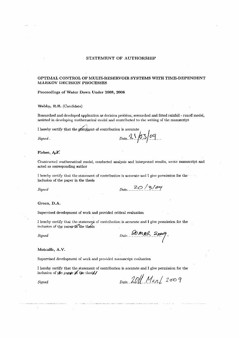
7. Fisher, AJ, Green, DA, Metcalfe, AV. and Webby, RB. 2008. OptimalControl of Multi-reservoir Systems with Time-dependent Markov Deci-sion Processes. Proceedings of Water Down Under 2008. Editors: MLambert, TM Daniell and M Leonard.

The corresponding short titles are:

1. Mekong - Tonle Sap

2. Lake Burley Griffin

3. Mekong - Delta

4. Crop selection

5. Sizing for desalination

6. Use of stormwater

7. Wivenhoe

xix

Chapter 1

Introduction

1.1 Research Problem

The supply and management of freshwater is becoming increasingly recognised

as a critical issue for the 21st century. This renewable resource is distributed

unevenly across the continents and may be either scarce or too abundant at

different times. Freshwater resources support ecosystems and human existence

and economic development. Water is used in the home, in agriculture, to gen-

erate electricity and as an input to industrial processes. Water bodies provide

a medium for transport and the setting for the ecological processes support-

ing fisheries. Water use by these different sectors may conflict through the

degradation of the resource for subsequent uses or through reductions in its

availability. Integrated management of a water resource involves a mixture of

scientific and engineering inputs as well as social, economic and environmental

factors. The managers of water resources, whether privately or publicly owned,

wish to make best use of their assets.

A mathematical model of the system - source, supply facilities and demand

- permits the use of optimisation techniques in finding the best potential so-

lutions for the allocation of the resource. By awarding them some monetary

value, social, economic and environmental factors can be included in a numer-

ical model. The objectives for a water allocation model commonly focus on

maximising expected net value however the avoidance of severe economic loss

should also be considered in decision making. A system that runs out of water

1

could face a social and economic catastrophe. So optimisation algorithms could

use multi-objective decision criteria, say, maximising expected net value and

minimising the risk of severe loss. One particular downside risk measure devel-

oped in finance is called Conditional Value-at-Risk (CVaR). It is a probability

based measure and can be used in water resource modelling in conjunction

with certain stochastic techniques and decision-making approaches.

The thesis has four aims;

• the development of mathematical models to represent water resource

management problems,

• the formulation and solution of optimisation problems associated with

these resources, particularly in a stochastic dynamic programming frame-

work,

• the application of CVaR to the assessment of water management policies,

and

• the comparison of optimal decisions found by the CVaR criterion with

those found by other decision-making criteria or rules.

These aims are central in the 7 publications in which I have reported my

research. Each paper takes a real-life water resource, develops a mathematical

model to represent the resource, and considers one or more typical water re-

source management problems inherent to the resource. The problems are cast

as a decision problem regarding either the allocation of the resource directly

or the allocation of funds to mitigate the impacts of excessive or deficient

resources. CVaR is the main criterion used to distinguish optimal decisions

but the conventional criterion of expected monetary value (EMV) is also con-

sidered, and, in some papers, the decisions obtained under both criteria are

compared. Table 1.1 lists the decisions and the criteria relevant to each paper.

2

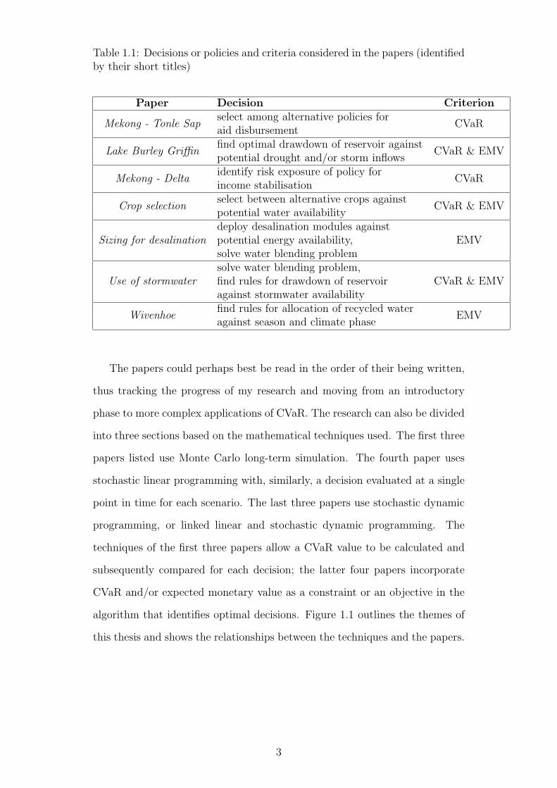
Table 1.1: Decisions or policies and criteria considered in the papers (identifiedby their short titles)

Paper Decision Criterion

Mekong - Tonle Sapselect among alternative policies for

CVaRaid disbursement

Lake Burley Griffinfind optimal drawdown of reservoir against

CVaR & EMVpotential drought and/or storm inflows

Mekong - Deltaidentify risk exposure of policy for

CVaRincome stabilisation

Crop selectionselect between alternative crops against

CVaR & EMVpotential water availability

Sizing for desalinationdeploy desalination modules against

EMVpotential energy availability,solve water blending problem

Use of stormwatersolve water blending problem,

CVaR & EMVfind rules for drawdown of reservoiragainst stormwater availability

Wivenhoefind rules for allocation of recycled water

EMVagainst season and climate phase

The papers could perhaps best be read in the order of their being written,

thus tracking the progress of my research and moving from an introductory

phase to more complex applications of CVaR. The research can also be divided

into three sections based on the mathematical techniques used. The first three

papers listed use Monte Carlo long-term simulation. The fourth paper uses

stochastic linear programming with, similarly, a decision evaluated at a single

point in time for each scenario. The last three papers use stochastic dynamic

programming, or linked linear and stochastic dynamic programming. The

techniques of the first three papers allow a CVaR value to be calculated and

subsequently compared for each decision; the latter four papers incorporate

CVaR and/or expected monetary value as a constraint or an objective in the

algorithm that identifies optimal decisions. Figure 1.1 outlines the themes of

this thesis and shows the relationships between the techniques and the papers.

3

desalination

Introduction to stochastic water management

Conditional Value!at!Risk

Monte Carlo simulation

Linear / Stochastic linear programming

selectionCrop

Mekong ! Tonle Sap

Lake Burley

Griffin

Mekong ! Delta

Wivenhoe

Stochastic dynamic programming

Useof

stormwater

Sizingfor

Figure 1.1: Research themes, mathematical techniques and associated papers

4

1.2 Stochastic Hydrology

Stochastic hydrology is the application of probability theory, especially that

pertaining to stochastic processes and statistics, to hydrologic systems. Such

systems often display spatial and temporal heterogeneity and coupled relation-

ships so that they are inherently complex. Even reasonably detailed physically

based models, such as SHETRAN, cannot emulate the spatial and temporal

heterogeneity typically found. Stochastic models can be used to account for

the errors in SHETRAN. Also, in many cases, much simpler conceptual models

of hydrologic systems suffice, again with stochastic models to account for the

errors.

A renowned early application of stochastic hydrology was the management

of water resources held in a reservoir (Moran, 1959). In general, reservoirs

provide multiple services: water supply for human consumption and for agri-

cultural or industrial requirements; hydropower generation; flood control pro-

tection; recreation; and the maintenance of ecological and environmental pro-

cesses. In many areas the most suitable sites for reservoir location have already

been developed, and water harvesting in these catchments is near the maxi-

mum possible. Population growth and increasing economic activity demand

that the available water be managed in an efficient manner. Management ob-

jectives for a reservoir may be maximisation of reliable yield or financial return,

or minimisation of cost of supply while meeting other goals.

Mathematical modelling, particularly operations research, is widely used

in solving these problems. Constraints and demands are quantitative, models

can represent the physical links between parts of the system and algorithms

can incorporate the stochastic and dynamic features of a system. Challenges

in modelling arise from the size and complexity of large systems - leading to

compromises in simplifying models while still capturing the relevant features

of the system - and the need to represent the stochastic elements of the system.

5

These stochastic elements are natural processes (rainfall, streamflow, . . . )

and the choice of a probability model to represent the stochastic elements

is influenced by the use to which it will be put, other practical arguments

and theoretical grounds but mainly on the basis of goodness of fit amongst

contending models. An outline of the approach to model selection used in the

analysis reported in this thesis is given in Figure 1.2.

select alternate model

extract descriptive statistics

estimate model parameters

assess model by residuals

choose initial modelsuitable for purpose

ismodel

yessatisfactory?no

Figure 1.2: A general approach to model fitting

The papers will show many instances of stochastic hydrology. Exam-

ples are: statistical characterisation of hydrologic variables such as rainfall

and streamflows, but also supply, demand and constraints in the linear pro-

grams; error modelled by probability distributions; and stochastic simulation

for the study of hydrologic systems under a range of inputs including cli-

mate change scenarios, to extend limited data sets, and for the assessment of

system responses under alternative management policies. Optimisation tech-

niques added to stochastic analysis provide a tool for decision-making in water

resource planning and operation. Table 1.2 presents a summary of the water

resource problems considered in the various papers which I have used stochas-

tic techniques to address.

6

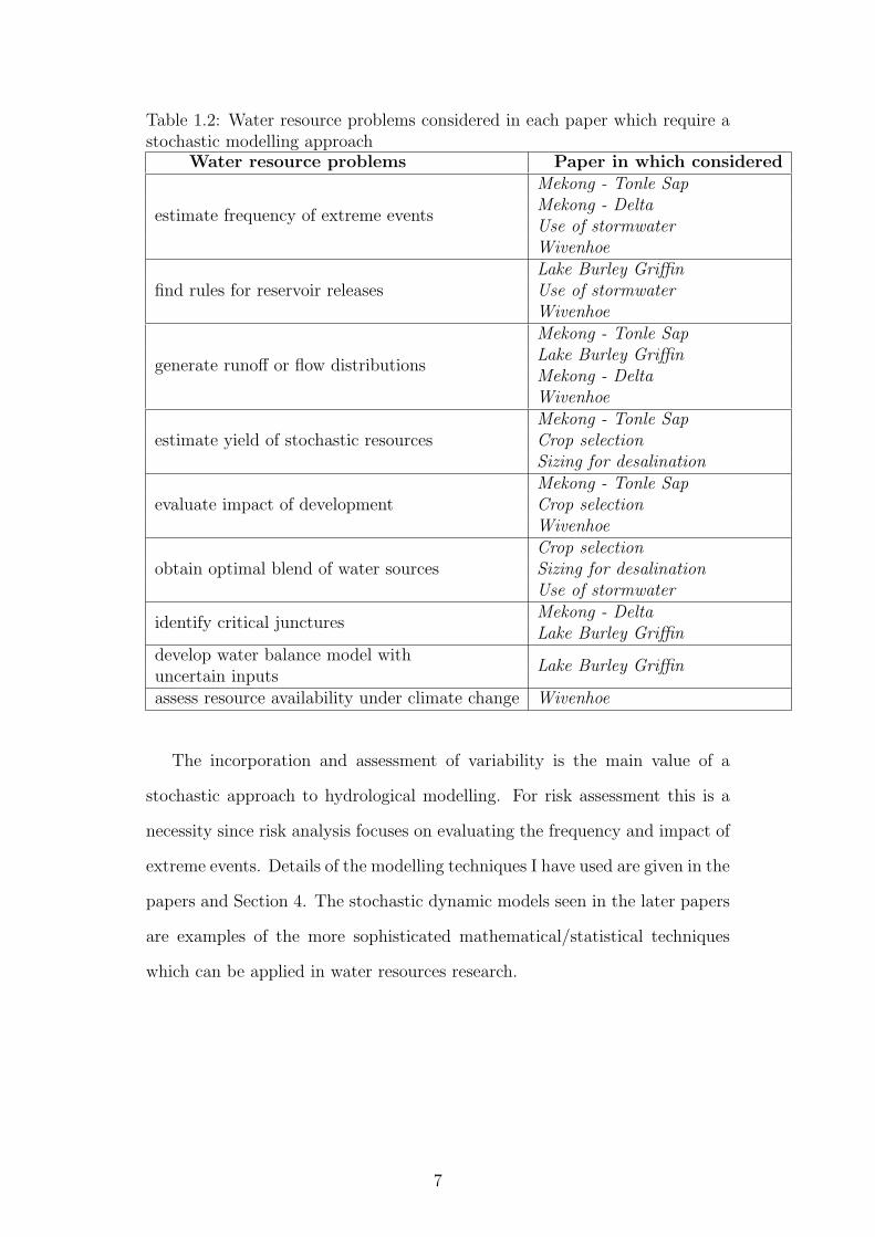
Table 1.2: Water resource problems considered in each paper which require astochastic modelling approach

Water resource problems Paper in which considered

estimate frequency of extreme events

Mekong - Tonle SapMekong - DeltaUse of stormwaterWivenhoe

find rules for reservoir releasesLake Burley GriffinUse of stormwaterWivenhoe

generate runoff or flow distributions

Mekong - Tonle SapLake Burley GriffinMekong - DeltaWivenhoe

estimate yield of stochastic resourcesMekong - Tonle SapCrop selectionSizing for desalination

evaluate impact of developmentMekong - Tonle SapCrop selectionWivenhoe

obtain optimal blend of water sourcesCrop selectionSizing for desalinationUse of stormwater

identify critical juncturesMekong - DeltaLake Burley Griffin

develop water balance model withLake Burley Griffin

uncertain inputsassess resource availability under climate change Wivenhoe

The incorporation and assessment of variability is the main value of a

stochastic approach to hydrological modelling. For risk assessment this is a

necessity since risk analysis focuses on evaluating the frequency and impact of

extreme events. Details of the modelling techniques I have used are given in the

papers and Section 4. The stochastic dynamic models seen in the later papers

are examples of the more sophisticated mathematical/statistical techniques

which can be applied in water resources research.

7

8

Chapter 2

Conditional Value-at-Risk

Aim

The concept of CVaR is central to five of the papers and could be used as an

alternative criterion in the other two. To the best of my knowledge the use

of CVaR in a water resources context was novel at the time the papers were

submitted for publication. Water resource researchers are typically familiar

with deterministic and stochastic decision making with expected monetary

value criteria but CVaR may be relatively unfamiliar so this chapter provides

a tutorial in CVaR.

Background

Conditional Value-at-Risk is a risk measure developed in finance for assessing

market risk. CVaR analysis assumes that market value, or changes in that

value, can be characterised by a probability distribution. All factors influ-

encing the value can, at least theoretically, be included when generating the

probability distribution. Then CVaR can be applied in any arena for which a

returns or loss distribution can be determined. CVaR was developed from the

quantile measure of risk Value-at-Risk (VaR) in order to obtain a risk measure

with improved practical and theoretical properties. VaR has become a stan-

dard for reporting market exposure in the financial area and is widely used by

trading organisations such as banks and securities firms, and their regulators

9

such as the Basel Committee on Banking Supervision. However, VaR (and

CVaR) is a general concept that can be applied to risk assessment in other

areas. Later, I briefly review applications of VaR and CVaR from the scientific

literature in the areas of insurance, agricultural production, electricity market

pricing and logistics. In this thesis, I demonstrate the application of CVaR to

water resources management.

In this chapter, I present Value-at-Risk and Conditional Value-at-Risk,

defining them and describing their application, methods of calculation, their

mathematical properties and the assumptions underlying their use.

2.1 Value-at-Risk

VaR is defined as the maximum loss expected to be incurred over a given time

horizon at a certain level of probability. If the loss distribution is continuous

VaR can be found as a quantile of the distribution. Its calculation may be

more complicated when the loss distribution is discontinuous (see equation

2.1). CVaR is defined as the expected loss given that the loss is greater than

or equal to the VaR value. Figure 2.1 is a graphical representation of a hypo-

thetical loss distribution with a long tail leading to the maximum loss. VaRα

has α% of the distribution to its left. CVaRα is the average of loss values from

VaRα to the maximum loss.

I illustrate the concept with a water resources example. Consider the wa-

ter holdings of a reservoir. The water body’s value can be calculated from its

provision of, say, power generation, irrigation, recreation, flood protection and

environmental services. The water body’s current volume and thus value is

known but its value at the end of the next three months is not known. The

change in value is a random variable and has an associated probability dis-

tribution. Call this distribution a loss distribution and note that a negative

10

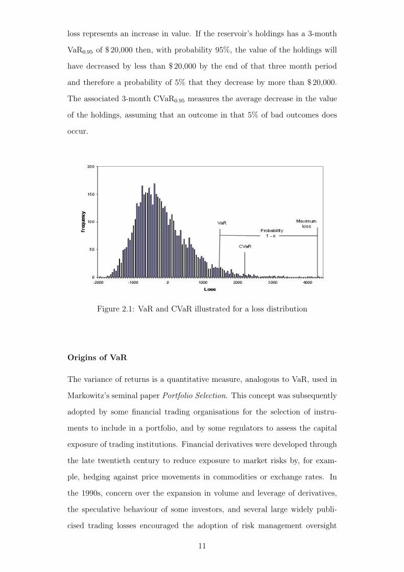
loss represents an increase in value. If the reservoir’s holdings has a 3-month

VaR0.95 of $ 20,000 then, with probability 95%, the value of the holdings will

have decreased by less than $ 20,000 by the end of that three month period

and therefore a probability of 5% that they decrease by more than $ 20,000.

The associated 3-month CVaR0.95 measures the average decrease in the value

of the holdings, assuming that an outcome in that 5% of bad outcomes does

occur.

Figure 2.1: VaR and CVaR illustrated for a loss distribution

Origins of VaR

The variance of returns is a quantitative measure, analogous to VaR, used in

Markowitz’s seminal paper Portfolio Selection. This concept was subsequently

adopted by some financial trading organisations for the selection of instru-

ments to include in a portfolio, and by some regulators to assess the capital

exposure of trading institutions. Financial derivatives were developed through

the late twentieth century to reduce exposure to market risks by, for exam-

ple, hedging against price movements in commodities or exchange rates. In

the 1990s, concern over the expansion in volume and leverage of derivatives,

the speculative behaviour of some investors, and several large widely publi-

cised trading losses encouraged the adoption of risk management oversight

11

of trading portfolios (Holton, 2003). Value-at-Risk was developed as a risk

measure for the derivatives market, notably by JP Morgan Chase, from 1994

(Holton, 2003). Regulators such as the Basel Committee on Banking Supervi-

sion moved to standardise risk appraisal and VaR methodology in particular.

VaR became one of the most popular methods for quantifying market risk and

has been widely adopted by trading organisations. VaR may not have helped

traders avoid the subprime mortgage and securities losses in 2008 since the

packaged debt was opaque regarding its true exposure (See Joe Nocera’s ar-

ticle at www.nytimes.com/2009/01/04/magazine/04risk-t). Similarly, Barings

Bank collapsed despite VaR oversight of its trading positions as certain trades

were concealed from risk managers. VaR can not overcome fraud.

Attributes of VaR

VaR’s attributes lie in three main areas. Firstly, it focuses on downside risk.

Cost-benefit analysis, an alternative risk approach, usually focuses on max-

imising the expected return of an investment, giving equal weight to potential

exceptional profits and large losses. VaR allows for the quantification of po-

tential loss alone, and thus measures downside risk. A firm’s holdings can

be adjusted to reduce the magnitude of potential losses, although this may

also mean a tradeoff in potential profit. Quantifying the risk allows decision

making to proceed in light of the risk nature of the investing firm. Secondly,

VaR summarises the risk associated with complex holdings in a single figure.

For example, a financial portfolio may contain derivatives that can generate

nonlinear returns relative to the value of underlying assets, making the port-

folio’s precise exposure to loss unclear. The probability distribution of returns

developed to calculate VaR incorporates any perceived effects on returns. The

combined effects, for the specified time period and probability level, are con-

densed into a distinct value. Thirdly, VaR is intuitive. VaR values are given

in monetary terms at specified probability levels. When calculated using the

same methods, VaR amounts for alternative investment scenarios or water

management policies are directly comparable.

12

Drawbacks of VaR

There are two main practical drawbacks to using VaR as a risk measure.

Firstly, VaR does not provide a measure of the potential losses exceeding the

VaR amount. For, say, a VaR0.99 or 0.99% VaR, losses in the 1% of the tail ex-

ceeding VaR may be only a little larger than VaR, or may be very much larger.

In effect, VaR at a given confidence level provides a lower bound for losses in

the tail of the loss distribution. It is typical of water resources that devastat-

ing losses may occur under conditions of drought, flood or other environmental

catastrophe, albeit at low probabilities. Secondly, VaR is difficult to optimise

algorithmically as the VaR values of different general loss distributions may

present many local minima which would have to be searched through to find

the global minimum. In finance, the assumption that the underlying variables

generating the returns are jointly normally distributed allows algorithms to

optimise VaR on the convex space of returns distributions. A further theoret-

ical deficiency of VaR is that it is not a coherent risk measure. Coherency is

discussed below.

2.2 Conditional Value-at-Risk

Conditional Value-at-Risk has the same attributes described above for VaR

but also overcomes VaR’s main drawbacks. Of most importance, CVaR does

give an estimate of the losses exceeding VaR. CVaR is a coherent risk measure.

An auxiliary function, presented by Rockafellar and Uryasev (2002), provides

an alternative method for minimising CVaR. The auxiliary function is convex

when the space of possible decisions generating loss are convex, and, in such

cases, can be represented as a linear optimisation problem. And while CVaR

may encapsulate the risk associated with a particular state of a system, deci-

sions are likely to be made against a number of benchmarks such as potential

profit or returns.

13

Coherency

Let Ω be a non-empty set whose elements, ω, are subsets of one or more out-

comes. An example with subsets of single elements is that of releases of water

from a reservoir in discrete units. Let P be a probability measure assigning

each ω a probability between 0 and 1, with P (Ω) = 1. The loss at the end of

a given time period for a subset in Ω can be denoted by the random variable

Z and the risk of Z is defined by some number ρ(Z).

The following four axioms for a coherent measure of risk were developed

by Artzner et al. (1999).

A measure of risk, ρ, is called a coherent measure of risk if it satisfies the

following conditions,

1. for all Z ∈ Ω and a ∈ R, ρ(Z + a) = ρ(Z) + a (translation-invariance),

2. for all Z1 and Z2 ∈ Ω, ρ(Z1 + Z2) ≤ ρ(Z1) + ρ(Z2) (subadditivity),

3. for all λ ≥ 0 and all Z ∈ Ω, ρ(λZ) = λρ(Z) (positive homogeneity),

4. for all Z1 and Z2 ∈ Ω with Z1 ≤ Z2, ρ(Z1) ≤ ρ(Z2) (monotonicity).

VaR, unless loss distributions are symmetrical, fails to meet the axiom of

subadditivity. This is a theoretical and intuitive failing. It means that the VaR

of a portfolio with two instruments may be greater than the sum of the indi-

vidual VaRs of the instruments. This is counter to the idea that diversification

of holdings should not increase losses, implied in the saying “don’t put all your

eggs in one basket”. An example to show the non-subadditivity of VaR follows.

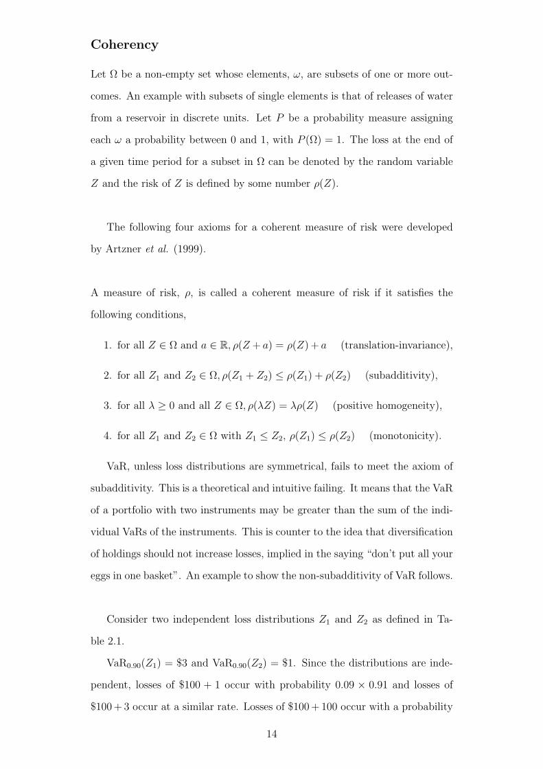
Consider two independent loss distributions Z1 and Z2 as defined in Ta-

ble 2.1.

VaR0.90(Z1) = $3 and VaR0.90(Z2) = $1. Since the distributions are inde-

pendent, losses of $100 + 1 occur with probability 0.09 × 0.91 and losses of

$100 + 3 occur at a similar rate. Losses of $100 + 100 occur with a probability

14

Table 2.1: Two loss distributions

probability of loss 0.5 0.4 0.01 0.09amount of loss ($) for Z1 3 3 3 100amount of loss ($) for Z2 1 1 1 100

of 0.092. These probabilities sum to 0.1719 so that P (Z1 + Z2 > 100) > 0.1

and VaR0.90(Z1 +Z2) > 100. So VaR0.90(Z1 +Z2) 6≤ VaR0.90(Z1)+VaR0.90(Z2)

and VaR fails the subadditivity axiom for this example.

By contrast, CVaR0.90(Z1) =3× 0.01 + 100× 0.09

1− 0.90= $90.3 and similarly

CVaR0.90(Z2) = $90.1. CVaR0.90(Z1) + CVaR0.90(Z2) = $180.4.

Now CVaR0.90(Z1+Z2) =0.0081× 200 + 0.0819× 103 + 0.01× 101

1− 0.90= $110.66.

We have that CVaR0.90(Z1 + Z2) ≤ CVaR0.90(Z1) + CVaR0.90(Z2).

Let Z be a random variable representing loss with g(z) as the probability

density function of Z and G(z) = P (Z ≤ z) as the cumulative density function.

CVaRα(z) = E[z | G(z) ≥ α] .

1. translation invariance

CVaRα(z + a) = E[z + a | G(z + a) ≥ α]

= E[z + a | G(z) + a ≥ α] .

The constant, a, appears on both sides of the conditional statement

above and so the expectation consists of the constant plus the conditional

expectation of the random variable

CVaRα(z + a) = a + E[z | G(z) ≥ α]

= a + CVaRα(z) .

2. subadditivity The expected value of a linear combination of two inde-

15

pendent random variables is given by E[Z1 + Z2] = E[Z1] + E[Z2].

CVaRα(z1 + z2) = E[z1 + z2 | G(z1 + z2) ≥ α]

= E[z1 | G(z1 + z2) ≥ α] + E[z2 | G(z1 + z2) ≥ α] .

Now CVaR is the expected loss given that the loss is greater than or

equal to VaR. Rewriting the first term on the right hand side of the

equation immediately above,

E[z1 | G(z1 +z2) ≥ α] = E[z1 | z1 +z2 ≥ VaRα] = E[z1 | z1 ≥ VaRα−z2]

The expected value of z1 given losses at least as large as VaRα− z2 must

be less than or equal to the expected losses given losses at least as large

as VaRα. That is

E[z1 | z1 ≥ VaRα − z2] ≤ E[z1 | z1 ≥ VaRα] .

The latter term is CVaR for the single distribution of Z1. A similar

argument shows that E[z2 | G(z1 + z2) ≥ α] ≤ E[z2 | z2 ≥ VaRα] and we

have

E[z1 | G(z1+z2) ≥ α]+E[z2 | G(z1+z2) ≥ α] ≤ E[z1 | G(z1) ≥ α]+E[z2 | G(z2) ≥ α]

or CVaRα(z1 + z2) ≤ CVaRα(z1) + CVaRα(z2).

3. positive homogeneity Now ρ(z) = c when z = some constant c.

CVaRα(λz) = E[λz | G(z) ≥ α]

= λE[z | G(z) ≥ α]

= λCVaRα(z) .

4. monotonicity To say that one random variable is less than another ran-

16

dom variable is to say that the ordered values that the first random

variable can take are individually less than those the second variable

may take. Then the expected value of a proportion of the first or-

dered distribution is less than the expected value of the same propor-

tion of the second ordered distribution. If the random variables are

said to be equal then their ordered values are identical. That is, given

Z1 ≤ Z2, ρ(Z1) ≤ ρ(Z2).

Definitions of VaR and CVaR

Let x ∈ X ⊂ Rn be a decision vector. In the financial arena, this would

typically be the number of units to hold of a particular enterprise in a share

portfolio. In water catchment terms, the decision could be the water level to

maintain in various reservoirs, possibly to drawdown a reservoir by a specified

amount. A decision vector would have elements representing every enterprise

in the portfolio, or every reservoir in the catchment model. Such a decision

typically occurs in response to a change in the value of another variable, call

this y.

Let y ∈ Y ⊂ Rm be a vector representing the values of a variable influ-

encing the decision variable. Such values could be movements in the foreign

exchange rate that may influence the market value of shares, or anticipated

increases in the water level of a reservoir following rainfall events in its catch-

ment. Of interest to shareholders and catchment managers is the effectiveness

of any decisions taken with respect to the available information on relevant

influential variables. The effectiveness of decisions can be estimated via a loss

function.

Let z = f(x, y) be a function that describes the loss generated by deci-

sion x and influential variable y. The values of y may come from a random

variable that has a known probability distribution (for example, the modified

gamma distribution for daily rainfall used in Lake Burley Griffin). In this case,

17

the loss, z, is a random variable with a different distribution for each value

of x. Note that while it is customary to underline vectors or write them in

bold font I have not done so with x and y. VaR and CVaR are defined for a

single element of vector x and, in discussing the definitions below, I will be

referring to a single element of x. For each such element, the influential vector

y will likely comprise several elements but I choose not to typeset y as a vector.

Losses are generally calculated over a defined time period. For example,

the loss of a share portfolio could be calculated at market close each day. The

portfolio’s loss is readily quantified in dollar terms and note that a negative loss

is more commonly called a profit. The value of water holdings in a catchment

depends on the nature of its proposed uses, such as power generation, irriga-

tion, domestic and industrial supply and environmental flows. The period over

which loss would be calculated in a water catchment could be relatively long,

perhaps quarterly or yearly decision horizons are appropriate for various uses.

Loss can be estimated for future periods by generating values for y from

the probability distributions of variables of influence. Then loss can be opti-

mised in the light of these predicted values against a range of values of the

decision variable, x. Simulations producing values of y will produce a range

of values of z for each x. A measure of risk (of loss) is a summary of the loss

distribution associated with decision x. Summary figures based on the spread

of a loss distribution include the standard deviation and VaR.

The definitions below follow those set out in Rockafellar and Uryasev

(2002).

The cumulative distribution function for loss is

Ψ(x, ζ) = Py | f(x, y) ≤ ζ,

18

where ζ is loss and Ψ(x, ·) is recalculated for every value of x. Ψ(x, ζ) is

non-decreasing with respect to ζ and is continuous from the right but not nec-

essarily from the left because of the possibility of jumps or discontinuities in

the loss distribution.

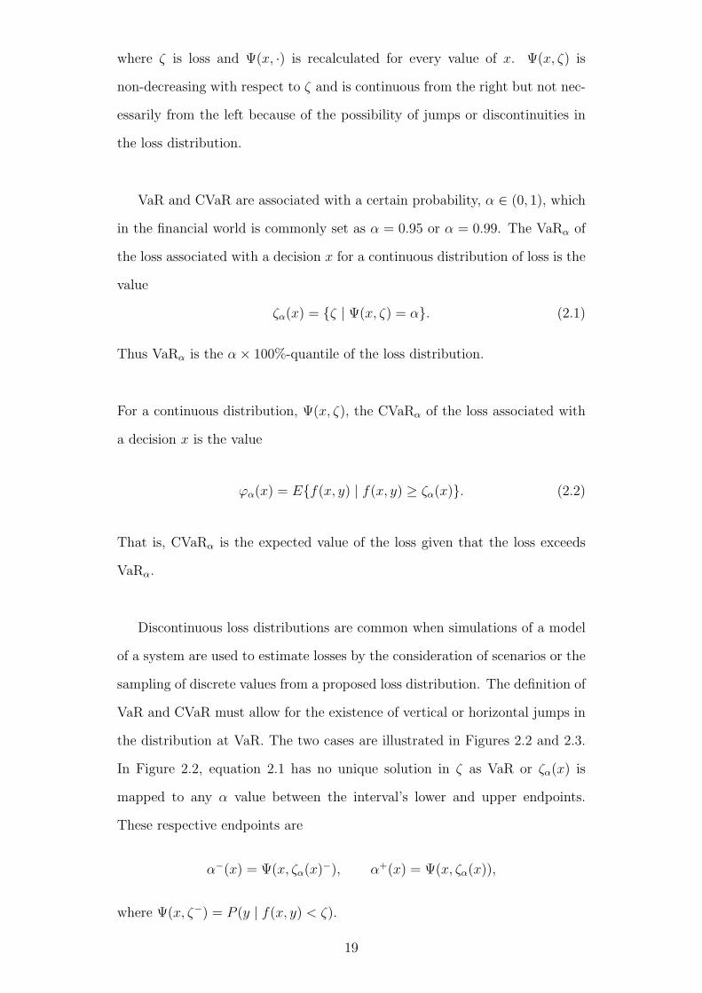
VaR and CVaR are associated with a certain probability, α ∈ (0, 1), which

in the financial world is commonly set as α = 0.95 or α = 0.99. The VaRα of

the loss associated with a decision x for a continuous distribution of loss is the

value

ζα(x) = ζ | Ψ(x, ζ) = α. (2.1)

Thus VaRα is the α× 100%-quantile of the loss distribution.

For a continuous distribution, Ψ(x, ζ), the CVaRα of the loss associated with

a decision x is the value

ϕα(x) = Ef(x, y) | f(x, y) ≥ ζα(x). (2.2)

That is, CVaRα is the expected value of the loss given that the loss exceeds

VaRα.

Discontinuous loss distributions are common when simulations of a model

of a system are used to estimate losses by the consideration of scenarios or the

sampling of discrete values from a proposed loss distribution. The definition of

VaR and CVaR must allow for the existence of vertical or horizontal jumps in

the distribution at VaR. The two cases are illustrated in Figures 2.2 and 2.3.

In Figure 2.2, equation 2.1 has no unique solution in ζ as VaR or ζα(x) is

mapped to any α value between the interval’s lower and upper endpoints.

These respective endpoints are

α−(x) = Ψ(x, ζα(x)−), α+(x) = Ψ(x, ζα(x)),

where Ψ(x, ζ−) = P (y | f(x, y) < ζ).

19

!!(x)

!+(x)

"(x,#)

#!(x) #

Figure 2.2: VaR at a vertical discontinuity

!

"+!(x)

#(x,")

"!(x) "

Figure 2.3: VaR at a horizontal discontinuity

In the case shown in Figure 2.3 equation 2.1 has infinitely many solutions

in ζ in the interval between ζα(x) and ζ+α (x).

For a general loss distribution, VaRα is defined as

ζα(x) = infζ | Ψ(x, ζ) ≥ α (2.3)

which is now unique for any P (loss < VaRα) = α.

In words, VaRα is the smallest loss that is greater than or equal to the mini-

20

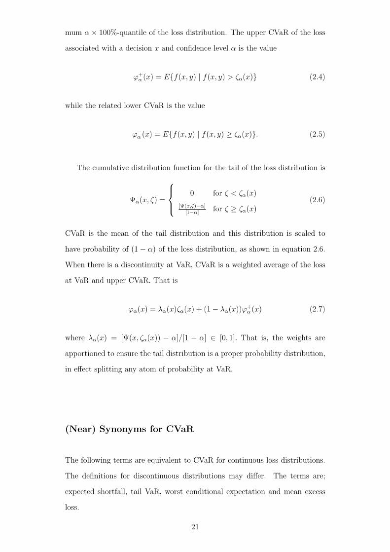
mum α× 100%-quantile of the loss distribution. The upper CVaR of the loss

associated with a decision x and confidence level α is the value

ϕ+α (x) = Ef(x, y) | f(x, y) > ζα(x) (2.4)

while the related lower CVaR is the value

ϕ−α (x) = Ef(x, y) | f(x, y) ≥ ζα(x). (2.5)

The cumulative distribution function for the tail of the loss distribution is

Ψα(x, ζ) =

0 for ζ < ζα(x)

[Ψ(x,ζ)−α][1−α]

for ζ ≥ ζα(x)(2.6)

CVaR is the mean of the tail distribution and this distribution is scaled to

have probability of (1 − α) of the loss distribution, as shown in equation 2.6.

When there is a discontinuity at VaR, CVaR is a weighted average of the loss

at VaR and upper CVaR. That is

ϕα(x) = λα(x)ζα(x) + (1− λα(x))ϕ+α (x) (2.7)

where λα(x) = [Ψ(x, ζα(x)) − α]/[1 − α] ∈ [0, 1]. That is, the weights are

apportioned to ensure the tail distribution is a proper probability distribution,

in effect splitting any atom of probability at VaR.

(Near) Synonyms for CVaR

The following terms are equivalent to CVaR for continuous loss distributions.

The definitions for discontinuous distributions may differ. The terms are;

expected shortfall, tail VaR, worst conditional expectation and mean excess

loss.

21

Parameters of VaR and CVaR

VaR and CVaR are specified in terms of two parameters. The first is the time

horizon for which VaR and CVaR are estimated. The time horizon often re-

lates to the liquidity period, that is, the time required to calculate the value of

the commodities concerned. For a portfolio of financial instruments this could

be one day, for insurance instruments this might be one year. The second pa-

rameter is the probability level at which VaR and CVaR are estimated. This

parameter usually reflects industry standards. For example, a company that

trades share market instruments may report a 1-day 95% VaR or CVaR. A

financial industry regulator may require market exposure reported as a 99%

VaR over a 2 week horizon. An insurance company may evaluate its exposure

to, say, flood damage payouts at 99.7% over one year. An application of VaR

to the cattle breeding market considered a 25 year horizon (Manfredo and

Leuthold, 1999b).

Assumptions of VaR and CVaR in practice

A major assumption in using these risk measures is that the model used to

develop the probability distribution for loss is as appropriate and accurate a

model as possible. The available information about potential loss is reduced

to a single VaR or CVaR value and decision makers and modellers would want

to have confidence in this value. The more complicated is the arrangement

of assets that generates returns, the more challenging is the task of produc-

ing an accurate model. CVaR particularly focuses on the rare events in the

tail of the returns distribution and so the model needs to accurately predict

the impact of these low frequency events. The accuracy of CVaR predictions

relies on precise values being assigned to the effects influential variables have

on a loss distribution. Of course, the assumption that the model is an accu-

rate representation of the system being studied is implicit in every such model.

22

Another assumption of the CVaR method is that the conditions which pro-

duced the historical data used to define the model and estimate parameters

for it will continue into the future. Stochastic variables can be represented by

probability distributions but the basic structure of the model, for example, the

elements comprising a portfolio, are fixed over the VaR or CVaR time horizon.

Factors which may influence the riskiness of a system and which may change

in their degree of influence, for example climate change impacts on water yield

over the life time of a dam, can be included in the model by the use of scenarios.

Writers from finance in explaining VaR, for example, (Holton, 2003), often

say that VaR applies only to (financially) liquid assets, that is, commodities

whose value is frequently tested in the market. An accurate value for a com-

modity improves the accuracy of predictions made on its potential change in

value. Furthermore, the precision of the most commonly used method of cal-

culating VaR, the variance-covariance method, relies on a detailed knowledge

of the variability of the commodity’s value, or of the variability of the strength

of influence of factors influencing that value. For many assets, models of their

values may be available, and these can provide reliable estimates of the value

of the assets. I have developed valuations myself in this work, relying on infor-

mation from people familiar with a particular water resource system, but also

use, and give the provenance of, valuations developed by other authors. Valu-

ations for water in the Murray-Darling Basin region of Australia are available

from the developing water trading market in this region.

2.3 Calculation of VaR and CVaR

Calculation of VaR

There are three common methods used to calculate VaR; the variance-covariance

method, historical simulation, and Monte Carlo simulation.

23

Variance-covariance

At its simplest, this method relies on two assumptions. Firstly, that the change

in value of a portfolio is a linear combination of the changes in value of the indi-

vidual elements or assets making up that portfolio, and, thus, that the portfolio

return is linearly dependent on the asset returns. Secondly, that returns of the

assets are jointly normally distributed. Then, the portfolio return is normally

distributed since a linear combination of jointly normally distributed variables

is itself normally distributed. An equation for VaR is formulated in terms of

the covariance matrix of the asset values. CVaR is the mean of the tail of

the distribution above the chosen quantile. Extensions of this method include

quadratic relationships between asset and portfolio returns and models that

include heteroschedasticity in variances over the time horizon considered.

The variance-covariance method requires the estimation of means, vari-

ances and covariances of asset returns. However, the assumption that asset

returns are (jointly) normally distributed is generally not well supported by

market data. The method is relatively easy to implement as data are readily

available for estimating the parameter values and it is straightforward to use

with a linear algebra software package (often required due to the large number

of individual elements making up a finance portfolio).

Historical simulation

Historical simulation is the simplest and most transparent method of calcu-

lating the risk measure. It entails using a record of previous changes in the

value of a portfolio or commodity, then applying these to its current value to

generate an empirical distribution for loss. For example, a financial company

may track historic changes in instrument values over a moving 100 trading day

period. VaR and CVaR are then calculated as the appropriate quantile and

mean of the tail of the empirical distribution.

24

The method makes no assumptions about the shape of the distribution,

thus avoiding the drawback of assumptions of normality for asset returns made

by the variance-covariance method. The method is easy to implement although

it can be computationally intensive for extensive portfolios. Using this method

requires the existence of suitable, large data sets. These are available for reg-

ularly traded commodities and financial instruments but are less available in

other areas. The method assumes that the next period of time is similar to the

historic period with respect to the influences on the future losses. As such, it

provides a retrospective indication of risk and is unable to incorporate views

on current and future trends in values.

Monte Carlo simulation

Monte Carlo (MC) simulation uses a model of the underlying process influenc-

ing an asset’s value to generate a suite of possible changes in the asset value.

For each iteration of the MC simulation, the process is (pseudo) randomly

simulated, the asset is revalued and the change in value is calculated. After

numerous iterations an empirical distribution of asset returns is built up. VaR

is calculated as the appropriate quantile of this distribution and CVaR as the

mean of the tail above VaR.

This method is conceptually simple but may be non-trivial to implement

since it requires that the process generating the losses be well understood and

modelled. Given this, the method is potentially more accurate than the others

listed here. Although historical data may be used to develop the model of the

system and estimate its parameters, MC simulation is able to incorporate hy-

pothesised future trends differing from the historical pattern. It is particularly

suited to modelling processes which generate non-linear returns.

25

Calculation of CVaR

In the case where there is a known probability distribution for loss, calculation

of CVaR requires the determination of the mean of the scaled tail distribution,

and this can be done analytically. Where the loss distribution is approxi-

mated by simulation, CVaR can be found through a straightforward numerical

method. Applications which use both these methods are found in the papers.

A scenario approach that generates a loss distribution may also allow CVaR to

be evaluated analytically. Another technique to calculate CVaR is described

in Rockafellar and Uryasev 2000. It relies on minimisation of their special

function.

CVaR (and VaR) is typically used in two ways. One involves the calcula-

tion of CVaR for several policies, with the policy generating the smallest CVaR

value favoured for implementation. The other is to set a specified amount for

CVaR and select between potential decisions making up a policy which to-

gether meet the criterion.

CVaR is a convex function with respect to decision x and, as Rockafellar

and Uryasev show, can be calculated as the minimum value with respect to ζ

of their special function

Fα(x, ζ) = ζ +1

1− αEy[f(x, y)− ζ]+ (2.8)

where

[x]+ =

x if x > 0

0 if x ≤ 0.

One advantage of using this function is that it is finite and convex and so

presents a straightforward minimisation problem.

A function, f(x), is convex on an interval [a, b] if for any two points x1 and

26

x2 in [a, b] and any λ where 0 ≤ λ ≥ 1

f(λx1 + (1− λ)x2) ≤ λf(x1) + (1− λ)f(x2).

Any local minimum of a convex function on [a, b] is also a global minimum.

27

2.4 CVaR and expected utility

CVaR analysis supports the making of rational economic decisions under un-

certainty. It evaluates expected losses over a given time horizon at a specified

probability and so clarifies the exposure to risk of loss if a particular decision

is made. CVaR values for any of the potential decisions considered in a given

situation are directly comparable (with the parameters of time horizon and

confidence level fixed). The ranking of CVaR values for various decisions iden-

tifies the risk-averse, economically optimal one. Alternately, a decision maker

can set an upper bound for CVaR and identify the decision with the highest

expected monetary value from the set of decisions which meet the bound. This

mathematical flexibility in estimating and establishing the scope of risk associ-

ated with a decision gives CVaR an advantage over the similarly risk-sensitive

decision-making criterion, expected utility.

Utility is a number that measures the desirability of an outcome. It is a

subjective measure, developed from Daniel Bernoulli’s observation that an in-

dividual’s own estimate of the worth of a risky venture is not the same as the

expected return of that venture. To calculate utility, we estimate the outcomes

or consequences from taking a particular decision, for all potential decisions

that might be considered in a given situation. Applying a coherent or rational

comparison, we rank these outcomes, the higher the ranking the more desirable

the outcome. A number, u ∈ (0, 1), is assigned to reflect the relative rankings.

The expected utility for a decision is the sum of the utilities for each outcome

multiplied by the probability of that outcome occurring, with the best deci-

sion being that which maximises expected utility. As long as the comparison

of alternatives is done rationally, utility theory allows the subjective valuation

of outcomes and the individual’s attitude to risk to be quantified, while at the

same time decision making is given a rational foundation (Lindley, 1971).

The difficulty in this procedure is that of assigning a rank to an outcome,

28

or equivalently, measuring its utility when each decision maker is assumed to

have a personal utility valuation, potentially changing with time. By asking

a person to rank a number of outcomes, we can build up a profile of their

utility and model it with a mathematical function (quadratic, exponential,

power,. . . ). Individuals with similar valuations could have their preferences

modelled by the same function, perhaps differing by a constant. There is con-

siderable discussion in the literature on the procedure and appropriate utility

functions. However, in carrying out the first step of the process, that is in

estimating the outcomes for all decisions and thus building up a distribution

of outcomes with associated probabilities, we have sufficient information to

calculate CVaR. For a risk-averse decision maker there is no need to proceed

further; to assign rankings to the outcomes or hypothesise a particular utility

function. CVaR gives a measure of the downside risk. An approach as sug-

gested in the first paragraph above incorporates the risk nature of an individual

into rational decision making, makes less assumptions and is computationally

easier.

2.5 CVaR and EMV

CVaR measures the risk of adverse events and, thus, focuses on one tail of

a loss distribution. EMV is a measure of the average value of the distribu-

tion. Both measures provide useful information to a manager and both could

be considered in a trade-off of risk of potential loss against expected return.

CVaR in general may not be a sufficient criterion for decision making on its

own. However, in water resource management where, say, failure to supply

may incur high costs, CVaR may be an important measure. In two of the

papers we consider loss distributions that are two-tailed and in these cases the

approach of minimising CVaR alone may be a feasible criterion for decision

making. Below I give a simple example of the comparison of CVaR and EMV.

29

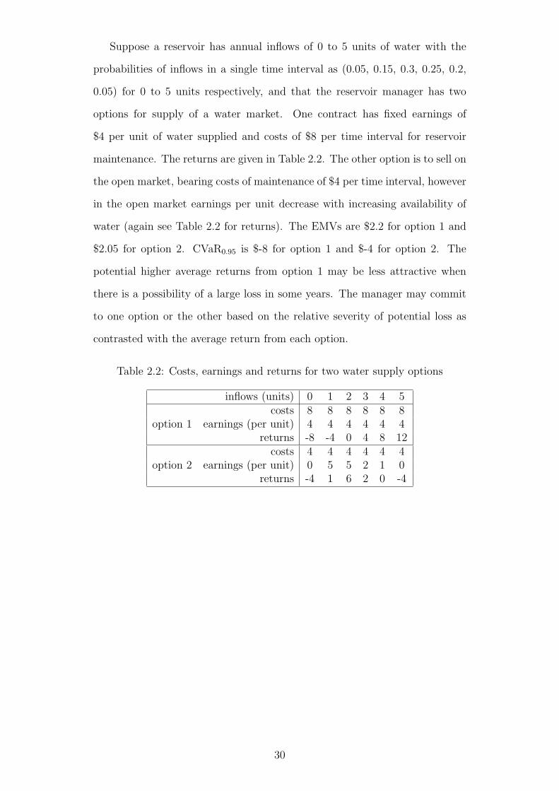
Suppose a reservoir has annual inflows of 0 to 5 units of water with the

probabilities of inflows in a single time interval as (0.05, 0.15, 0.3, 0.25, 0.2,

0.05) for 0 to 5 units respectively, and that the reservoir manager has two

options for supply of a water market. One contract has fixed earnings of

$4 per unit of water supplied and costs of $8 per time interval for reservoir

maintenance. The returns are given in Table 2.2. The other option is to sell on

the open market, bearing costs of maintenance of $4 per time interval, however

in the open market earnings per unit decrease with increasing availability of

water (again see Table 2.2 for returns). The EMVs are $2.2 for option 1 and

$2.05 for option 2. CVaR0.95 is $-8 for option 1 and $-4 for option 2. The

potential higher average returns from option 1 may be less attractive when

there is a possibility of a large loss in some years. The manager may commit

to one option or the other based on the relative severity of potential loss as

contrasted with the average return from each option.

Table 2.2: Costs, earnings and returns for two water supply options

inflows (units) 0 1 2 3 4 5

option 1costs 8 8 8 8 8 8

earnings (per unit) 4 4 4 4 4 4returns -8 -4 0 4 8 12

option 2costs 4 4 4 4 4 4

earnings (per unit) 0 5 5 2 1 0returns -4 1 6 2 0 -4

30

Chapter 3

Literature Review

3.1 Applications of VaR and CVaR other than

in water resources

The main area of implementation of VaR and CVaR is in the financial world.

However, several researchers, noting the success of VaR in the financial indus-

try, are applying it in other fields.

Manfredo and Leuthold (1999a) recognised potential applications for VaR

in agricultural enterprises including, risk disclosure for credit providers, the

assessment of crop marketing strategies and the assessment of an individual

firm’s production against future climate and market uncertainty. In another

paper (Manfredo and Leuthold, 1999b) these authors applied VaR to a feedlot

enterprise, recommending its use in the evaluation of risk minimisation strate-

gies.

Manfredo and Leuthold (1999a) noted that several agricultural commodi-

ties (for example, corn) are regularly traded in large markets and, thus, val-

uations for these commodities are robust and suitable for standard VaR es-

timation techniques developed in the financial industry. The paper describes

nonparametric and parametric VaR (the usual method described in books on

VaR where returns are assumed to follow a normal distribution). VaR and

31

CVaR are then readily calculated as quantiles of the distribution. Nonpara-

metric VaR methods develop an empirical distribution for loss and estimate

VaR or CVaR by simulation. Under the assumption of normality the prob-

lem becomes one of forecasting the portfolio standard deviation (or volatility)

and estimating the correlations between individual assets and hence portfolio

volatility. For this analysis, a history of market price movements is required,

particularly extreme changes in price that characterise the tails of the returns

or loss distribution. A major criticism of parametric VaR is that portfolio re-

turns are generally not normally distributed, particularly when portfolios con-

tain derivatives. Leptokurtosis in the probability distribution can distort VaR

and CVaR estimates (and transgresses the assumption of normality). Annual

maximum or minimum river flows are commonly described by extreme value

distributions which have longer tails than the normal distribution. Another as-

sumption underpinning this method is that estimated market parameters hold

over the length of the analysis period. While a risk horizon for VaR in the

financial world can be as short as one day ahead, risk horizons in agriculture

and water resource management would often be longer. The assumptions may

be justified in the context of certain well-developed commodity markets but

parametric techniques may not be reasonably applied in the water resources

arena.

Pruzzo et al. (2003) compared a risk measure based on CVaR with expected

returns to discriminate between bulls selected for breeding, demonstrating that

decisions based solely on expected return may not select the best potential out-

come. They used parametric techniques with a 20 year time horizon. Schnitkey

et al. (2004) described the use of VaR in crop insurance and demonstrated

the difficulty of using VaR to evaluate alternatives when loss distributions

are non-smooth. The authors then showed why CVaR should be preferred to

VaR. They investigated the trade-off between minimising CVaR and maximis-

ing EMV and found it to be strongly negative for α = 0.99. Liu et al. (2008)

assessed crop insurance under climate variability, identifying the optimal strat-

32

egy among a limited set using a linear program and a CVaR constraint. Note

that the linear program includes the objective of maximising expected return

while not exceeding a specified potential loss which was characterised by CVaR.

An industry which recently has seen the development of competitive mar-

kets in many developed countries is that of electricity generation. Several

researchers have pointed out the high spot price volatility in this market and

demonstrated the application of VaR and/or CVaR to the industry. Dahlgren

et al. (2003) gave a tutorial in the use of VaR and CVaR as risk measures for

electricity portfolio trading. They note differences in the financial and elec-

tricity markets and emphasise the alternative basis (to maximising expected

profit) for decision making of minimising any potential loss. They demonstrate

that optimising a portfolio to minimise CVaR may provide a portfolio that is

less exposed to extreme losses than merely optimising with a minimum VaR

as an objective. They also point out that if a finite number of scenarios (to

model loss positions) is used, the optimisation of CVaR can be represented as

a linear program on which existing techniques can be used. Das and Wollen-

berg (2005) point out the need for companies to avoid large losses and thus

the need to carry out risk management. In simulations incorporating linear

and nonlinear effects on loss, they generate nonsmooth, empirical loss distri-

butions and use VaR to distinguish strategies for generators with different risk

profiles (that is, different acceptance levels for risk). Carrion et al. (2007)

wrote a stochastic integer linear program to determine the optimal decisions

for a large electricity consumer with some self-production capacity. They use

scenarios to reduce the dimensions of the problem and represent the stochastic

pool price with ARIMA models, aggregated to reduce dimensionality. CVaR is

included as a constraint in the linear program using the discrete linear version

of Rockafellar and Uryasev’s special function. The authors set a constant value

for α but weight the constraint to represent a range of risk attitude (β ∈ [0,∞)

with β = 0 as being risk neutral – this model does not accommodate the risk

taker). A plot of the expected cost of electricity against the weight suggests

33

an exponential relationship between risk attitude and expected cost.

Oil is traded in a relatively open market that occasionally sees volatile

price changes and the need for companies to avoid excessive loss. Cabedo and

Moya (2003) compared parametric and nonparametric methods for calculat-

ing loss distributions in developing a method for estimating VaR that they

showed to be efficient and consistent with oil price changes over a 12 month

period. In a market of less liquidity, Alonso-Ayuso et al. (2005) used VaR in

a product selection and plant dimensioning (PSPD) problem. In this case, ex-

pected net profit and Var were implemented as objectives in a linear program.

The authors compared the results from a deterministic setting of the problem

with a stochastic dynamic programming approach over multiple periods and

found that the SDP setting allowed adverse loss conditions to be identified

and avoided. A similar PSPD problem is presented by Aseeri and Bagajewicz

(2004). They demonstrate the advantage of identifying the tradeoff between

potential profit and risk exposure using VaR and an equivalent profit measure

for the upper tail of an empirical returns distribution. These measures permit

a systematic comparison of risk exposure and potential profit, enabling a risk-

averse or risk-taker investor to identify a preferred position. Sodhi (2005) also

uses VaR in a PSPD problem, solved in a linear program. Fang et al. (2004)

use conventional techniques from the chemical process industry to develop a

ranked list of risks faced by a process. After allocating values to various sce-

narios representing the risks, they apply VaR to identify priority areas for risk

reduction.

VaR or CVaR is seen as having a wide applicability for risk assessment

and as a criterion for informed decision making. Several authors advise that

a broad set of measures should be used to evaluate risky propositions and

some recognise CVaR as a superior measure to VaR. Cohen and Elliott (2008)

show that coherent risk measures in a dynamic program are a consistent risk

measure across the time horizon of the program.

34

3.2 Optimisation in water resource applications

Many optimisation techniques have been applied to typical water resource

problems such as reservoir operation. The techniques include: variants of

stochastic programming such as multi-stage, chance-constrained and dynamic

programming; stochastic linear programming; the use of fuzzy sets in conjunc-

tion with dynamic programming; optimal control theory; neural networks and

genetic algorithms; Bayesian networks; and scenario simulation with sensitiv-

ity analysis. Several authors, for example Yeh (1985, 1992), Simonovic (1992)

and Labadie (2004), reviewed the application of optimisation techniques in

water resource management.

Labadie (2004) describes the problem facing managers of reservoir systems

and gives an overview of the optimisation methods that have been applied

to multiple reservoir systems. He remarks on the strengths and weaknesses

of each approach, mentioning efforts from the literature on how to overcome

difficulties. Dynamic programming and SDP are specifically discussed along

with the techniques used to overcome the large state spaces encountered with

SDP.

Archibald et al. (1997) developed a technique to reduce the representa-

tional complexity of SDP applied to a multireservior system by subdividing

the system into the reservoir currently under scrutiny and an aggregate of

those reservoirs upstream and those downstream. Each reservoir is then con-

sidered in turn. The authors compared results obtained from this technique

with those obtained from a discretisation of the full system and demonstrated

that although aggregation loses information about the system, policies identi-

fied by this method were close to optimal. This model is extended in a later

paper (Archibald et al. (2005)) which reduces the dimensionality of the prob-

lem by considering one reservoir in detail while partitioning the holdings of

other reservoirs in the network into broad typical states. The advantage of

35

this technique is that it allows the individual characteristics (head for electric-

ity generation, potential flooding impact) of reservoirs to be considered.

Kerr et al. (1998) applied SDP to a single reservoir and compared policies

obtained under a risk averse approach to those obtained when maximising net

wealth over the time horizon. The authors use utility curves to represent risk

natures (avoiders, takers and those adopting a neutral position). They found

that a risk averse approach lessens the opportunity for high wealth and de-

creases overall wealth as compared to risk neutral behaviour. It also leads to

different behaviour in storage levels of reservoirs. Turgeon (2005) develops a

program to define rules for optimal yearly operation while taking account of

daily inflow characteristics, particularly persistence of rainfall patterns. Sepa-

rate rules are given for situations when reservoir levels are low or high, to deal

with short term inflow behaviour, while a dynamic program finds the optimal

release of water for the longer term. Yurdusev and O’Connell (2004) incorpo-

rate environmental concerns over water resource decisions into water resource

planning by weighting the various planning options in regard to their envi-

ronmental outcomes. A composite environmental index is used to integrate

environmental costs and benefits. The approach requires an economic valua-

tion of these costs and benefits so that the index can be included along with

economic outcomes in the objective function of the optimisation algorithm.

3.3 CVaR as a criterion in water resources

management

Since submitting my papers Yamout et al. (2007) compared the results of

five models written to optimise the allocation of water in an irrigation project.

Source availability was described by two normal distributions. The authors de-

velop deterministic and stochastic versions of an integer linear program. The

deterministic versions allocate water to minimise expected cost, either using

36

the mean of the distributions or the mean value of multiple allocation scenar-

ios. The stochastic versions are based on a two stage stochastic program with

recourse, initially with the objective of minimising cost, then of minimising

CVaR, and finally constraining CVaR while minimising cost. The authors note

that minimising expected cost does not take into account the consequences of

extreme events. They find that the deterministic version underestimates losses

while the stochastic one provides a potentially better representation of real-life

conditions. Minimising CVaR as the objective controls large losses in the tail

but does not efficiently allocate water to minimise all costs, while constraining

CVaR and minimising costs allows for control of large loss events and low loss

events.

37

38

Chapter 4

Synthesis

The following section is a description of each paper and its contribution to the

aims of the research project, which were;

• the development of mathematical models to represent typical water re-

source management problems,

• the formulation and solution of optimisation problems associated with

these resources, particularly in a stochastic dynamic programming frame-

work,

• the application of CVaR to the assessment of water management policies,

and

• the comparison of optimal policies found by the CVaR criterion with

those found by other decision-making criteria or rules.

Mekong - Tonle Sap

As the monsoon season proceeds in South East Asia, water fills the channels

of the Mekong River then inundates the flood plain, carrying the hatchlings of

migratory fish to complete their growth in the rich shallow floodwater. The

Tonle Sap connects the Great Lake of central Cambodia to the Mekong River,

reversing its direction of flow during the wet season so that it bears nutrients

and hatchlings from the Mekong mainstream to their nursery in the much-

expanded Great Lake. As the floodwaters recede and the Tonle Sap again

39

flows toward the sea, the Dai fishery operates on the river. The productivity

of this fishery is an indicator of the catch for the whole of Cambodia’s inland

fisheries, and these fisheries provide up to one tenth of Cambodia’s GDP and

up to three quarters of the protein intake of its people. A systematic reduction

in the flood hydrograph means a reduction in fishery income and, depending

on the magnitude of the reduction, a call on international aid agencies for re-

lief. One facet of this paper is the development of a model for the valuation of

Cambodia’s inland fishery catch; another is the risk analysis of aid disburse-

ment policies.

The latter strand of the paper develops through an introduction of the risk

measures; the generation of loss distributions through scenarios; the calcula-

tion of CVaR for continuous and discontinuous loss distributions by analytic

and simulation techniques; and a demonstration of the use of CVaR as a deci-

sion criterion for choosing between alternative policies.

The issues described in the paper around the Cambodian inland fishery and

fishers are of practical and topical importance. Those main issues are; the de-

pendence of the fishery on the annual flooding regime of the Mekong river and

the potential impact of dam development upstream of the Tonle Sap / Great

Lake fishery. I developed models for fish catch, catch valuation and river flows

from data supplied by researchers working in the Mekong Basin, and generated

the aid budget scenarios from reports of aid agencies active in South East Asia.

I demonstrate two techniques for calculating VaR and CVaR. The analytic

method requires the development of a known distribution for loss, from which

the risk measures can be found in terms of the distribution parameters. This

can only be done for the simplest models. In the second technique, Monte

Carlo simulation, artificial sequences of data are generated and an empirical

distribution for loss built up. Initially, we used a uniform distribution to model

river flood volume as, through the assumed linear relationships between river

40

flow and catch, and catch and catch valuation, we obtained a uniform distribu-

tion for loss. Then the calculation of VaR and CVaR is straightforward using

parametric methods, that is, directly using the definitions of the risk measures.

Following this, we simulate a loss distribution based on the earlier model but

including a distribution for errors in the regression of catch on flood volume.

To calculate VaR and CVaR from this empirical distribution, the simulated

losses are ordered, the α quantile of the distribution identified - this is VaR,

and the mean of the losses greater than or equal to VaR calculated - this is

CVaR.

Thus far I considered the loss, relative to average earnings, to the fishing

community if the seasonal flood is below average, that is, for deficient floods,

and demonstrated the calculation of CVaR. This was a straightforward calcu-

lation since the loss distribution is continuous. However, the precise definition

of CVaR allows for discontinuities in the loss distribution, and such discontinu-

ities arise in practice with aid schedules when calculating the donor’s risk. In

the first schedule presented in the paper, aid increases linearly with decreasing

flood volume except for a jump at the lower 5% quantile of the flood distri-

bution. In the second schedule, aid is piece-wise linear but remains constant

over a range of flood volumes. In the third schedule aid has jumps but is

constant between jumps. The distributions and the VaR value are depicted in

figures to show the definition of VaR graphically. The calculation of CVaR for

discontinuous distributions is shown, that is, CVaR is a combination of VaR

multiplied by the proportion of the atom of probability sited at VaR plus the

mean value of losses greater than VaR.

The schedules for aid disbursement are intended as representations of possi-

ble schedules. Given the economic model for the fishery, the schedules generate

discontinuous distributions. Many real-life applications would display such dis-

tributions. An assumption of normality of losses is not applicable here, but we

demonstrate how CVaR can be calculated for these non-normal distributions.

41

Many more than three aid disbursement schedules could have been written.

However, the selected schedules display the principal types of discontinuities

in loss distributions.

The principal advantage of VaR over CVaR is demonstrated by these exam-

ples. That is, for heavy-tailed distributions VaR is not an appropriate measure

of risk as it may seriously underestimate the exposure to loss.

Three aid disbursement schedules, which have a common cap of 2 billion

Riel, are compared in terms of their CVaR values. This is a common use of VaR

in finance. An investment portfolio may be required to meet a maximum VaR

value, or the portfolio with the minimum VaR may be selected from a number

of portfolios. It would be natural to model and evaluate possible exposure

to loss under promised aid schedules, as for insurance policies guaranteeing

redemption of agricultural loss. The adequacy of aid policies to alleviate suf-

fering is important in the event of a deficient flood season occurring, and a

CVaR analysis of the potential demand on donors under various aid schedules

is appropriate during planning for such events.

The paper concludes with alternative models offered for fishery catch against

flood volume, and for flood volume, the latter model being more realistic than

the earlier uniform distribution for flood volume. VaR and CVaR are calcu-

lated by Monte Carlo sampling from the distributions. This same technique is

used to calculate VaR and CVaR in the next two papers.

Lake Burley Griffin

Lake Burley Griffin is a large artificial lake designed as the centrepiece of the

new capital of Australia. At its ideal level, lake water laps the edges of lawns

leading up to the parliamentary buildings and furnishes reflections of many of

Canberra’s political and cultural sites. The lake is also a facility for more ac-

42

tive uses such as rowing and sailing, and a support for water-related ecosystem

processes.

The principal management imperative of Lake Burley Griffin is mainte-

nance of the lake level close to its reference level, that is, with the lake near

full. However there are good reasons for making releases: to provide environ-

mental flows; to irrigate lake surrounds; and for temporary floodwater deten-

tion. Thus there are conflicting objectives in lake management; in retaining or

releasing water. To gain insight into any trade-off between these objectives I

developed a mathematical model for daily water balance and rules for releases.

It is necessary to ascribe monetary values to the outcomes of competing

objectives if quantitative management decisions are to be made. Thus a sup-

porting model calculates values for lake holdings, including environmental and

aesthetic goals, withdrawals, and benefits or penalties for downstream releases.

Simulation of the water balance model at a daily time step allows a distribu-

tion of monetary values of benefits to be built up and measures of loss of value

to be calculated.

There is an extensive literature on the management of single or multiple

reservoirs. Generally these give management policies in the form of rules for

the release of water from a reservoir, often based on maximising the expected

return from release or retention of the water. An alternative basis for the

comparison of policies is a CVaR analysis of potential losses incurred under

those policies. Having introduced CVaR in Mekong - Tonle Sap, in this paper

I make comparisons of the reservoir release rules from using CVaR and EMV

as criteria.

The decision problem has two aspects. The first is to balance amenity,

which requires the lake to be near full, against downstream environmental

uses of the water and irrigation. The second is that the lake can provide some

43

flood detention if it is drawn down in anticipation of large inflows. Two scenar-

ios are considered, the first being the usual operating conditions in the driest

month of the year. The decision variable is the lake height at which to halt

release of water. The second is when high inflows are expected from reliable

short term weather forecasts or known from real time monitoring of upstream

rain gauges. The decision variable is the lake height to be achieved by draw

down.

The daily water balance model for Lake Burley Griffin has deterministic

and stochastic inputs. The latter is a two stage stochastic process for rainfall,

rainfall being scaled to runoff. A homogeneous Markov chain was developed

from a rainfall record with the 2 - state transition matrix representing the

conditional probabilities of moving from a dry day to a wet day or vice versa.

The second random variable takes positive values representing the amount of

rain on a wet day, the values being instances of a fitted Gamma distribution

for rainfall. Withdrawals of water are deterministic, for example spill above a

certain lake height, or are dependent on water height, for example abstractions

for irrigation. The water balance equation allows for weekly totals of releases

to be monitored so that daily management policies take into account longer

term management issues.

The model is run for repeated Februaries, since February is the month

with lowest inflows to the lake. However the climate of the region does pro-

duce rare high inflows in that month. The two situations, of chronic low inflows

and acute high inflows, are important to lake management.

Lake Burley Griffin is not a reservoir in private ownership dedicated to one

principal use such as electricity generation or storage of irrigation supplies.

Rather, it is a public body of water with conflicting claims on its use. How-

ever it is managed by a single statutory authority which can prioritise uses. In

order to carry out a CVaR analysis, values for the water holdings of the reser-

44

voir must be determined. A manager from the statutory authority assisted

me in developing valuations for water height of the lake for its abstraction,

amenity and recreational values. I developed mathematical expressions for the

wetlands value of the lake, for the value of environmental flows, and for losses

due to downstream flooding from literature reviews and expert advice.

For the first scenario, the CVaR criterion indicates an optimum level of

0.3 m below reference level at which to halt releases. In contrast, under the

EMV criterion, the expected loss decreases as the height below reference level

increases, although the decrease is slight once a level of 0.5 m below has been

reached. The model identified the maximum EMV at 1.0 m below reference

level. CVaR is more influenced by the potential loss of amenity, which includes

structural damage to the lake retaining walls, than is EMV. The lower level in-

dicated by the EMV criterion is a consequence of losses that arise from failing

to make environmental flows rather than the possible reduction in flood losses.

It is fortuitous that in this case the EMV criterion happens to provide more

protection against the largest loss generated in the simulation, $29.2 × 106.

However, the CVaR criterion does take account of the flooding costs. If the

high costs associated with flooding, which is rather unlikely, are ignored, the

CVaR criterion indicates a draw down limit of 0.23 m rather than 0.3 m.

When rainfall events of greater than 10 mm over the entire small catch-

ment are reliably forecast, the CVaR and EMV analysis agreed that lake levels

should be drawn down to 0.2 m below reference level (rainfall just greater than

10 mm raises lake level by approximately 0.135 m). Knowledge of impending

rainfall and the potential costs of flooding means that the downside risk is

paramount to both CVaR and EMV under this scenario.

CVaR favours a risk averse strategy rather than one which aims to maximise

EMV. There is some cost or potential return forgone in risk aversion; this can

be calculated for the first scenario of this application as EMV(min EMV criterion)−

45

EMV(min CVaR criterion) = EMV(1.0 m below) - EMV(0.3 m below) = 1.59−

1.65 = $0.06 (all numbers times 106).

Referring back to the aims of the thesis, this paper demonstrated a math-

ematical model to determine the optimal policy for releases from a reservoir.

This is a common problem in water resource management and the model, with

parameters suitably adjusted, could be applied to other single reservoir sys-

tems. Long term simulation is a practical optimisation strategy when there is

only one decision variable. More complex models are considered in subsequent

papers where techniques such as stochastic linear programming are applied.

Furthermore, the paper demonstrated the use of CVaR for developing optimal

management rules for release or retention of water in a reservoir. A second

purpose was the comparison of optimal policies found by an EMV criterion

and those found using a CVaR criterion. Either criterion could reasonably be

adopted by management, but a specific level below which releases are halted

might be appealing. Alternatively, a more complex decision rule involving re-

ductions in releases at various lake levels might be investigated. The fact that

losses can arise from both high and low lake levels has the interesting con-

sequence that, in this specific case, EMV fortuitously gives more protection

against the maximum potential loss.

Mekong - Delta

The Mekong Delta is a low-lying plain with the multiple braided channels typ-

ical of a large river delta. Annual inundation of the land in the wet season

replenishes soil moisture and nutrients, and renews a socio-economic cycle that

has made the Delta a region of dense population and high agricultural produc-

tivity. A good wet season has floods between an upper excessive threshold and

a lower deficient one. Risk and loss are experienced when floods are above or

below these respective thresholds. In this paper I develop a statistical model to

characterise flood behaviour, simulate flood seasons to build up a distribution

46

of the costs of extreme floods, and demonstrate the use of CVaR in estimating

the potential exposure of a crop insurance scheme to mitigate these costs.

Mekong - Delta is an extension in location and theme of Mekong - Tonle

Sap. In particular, the new paper extends the model for wet season flood vol-

umes at Kratie in the Lower Mekong. The earlier paper presented two models

for the flows. An initial simple model permitted a step through of the ana-

lytical calculation of CVaR. Later we showed that the flows are well-modelled

by a normal distribution, and CVaR was calculated empirically. Now, in a

further refinement to the model, wet season flows are characterised in terms

of two key hydrological features: peak discharge and seasonal volume. Peak

discharge indicates the area and depth of inundation, producing the potential

acute damage of the storm surge; seasonal volume indicates the duration of

inundation, causing longer-term effects of prolonged saturation. This bivariate

description of flood behaviour is an improved indicator of flood impact.

The form of the joint distribution is unknown but I can write down equa-

tions for its conditional distributions – that is, the peak discharge associated

with a particular flood volume and the flood volume associated with a certain

peak discharge – by regressing one variable on the other. These are conditional

distributions, not deterministic single values and so the range of, for example,

flood volumes for a particular peak discharge are modelled by developing an

appropriate error distribution. Analysis showed that variability in peak dis-

charge followed a Gumbel distribution and, as mentioned earlier, wet season

flood volume is well-modelled by a normal distribution. The conditional distri-

butions allow a sampling procedure, known as an empirical Gibbs sampler, to

generate a sequence of peak discharge, seasonal volume pairs from the bivari-

ate distribution. These are input to the second stage of the simulation model

- estimation of the monetary effects of the annual flood.

Flooding in the Mekong Delta has a two-tailed effect. The model calculates

47

losses associated with deficient floods, and damages associated with excessive

floods. I made use of a model for damage due to excessive peak discharge

developed by researchers in the Delta, adjusting it to allow for the bivariate

distribution for wet season flows. Other reports and local expert knowledge

guided me in constructing a model for losses due to deficient floods. The bi-

variate distribution of wet season flows means that each flood falls into one or

the other of these categories or, rarely, both when, for example, a wet season

of low overall flows experiences a period of high peak flows.

Simulating wet season flows, the model generates two empirical distribu-

tions, one for losses due to deficient flood seasons, and one for damages due

to excessive flood seasons. Usually one or the other of these is zero. A third

distribution, cost, is the maximum of loss or damage for each year. CVaR is

empirically found by sorting the simulated cost values and finding the VaR

quantile – here, the value with 20% of the distribution above it – and then

the mean of the values greater than or equal to VaR. VaR and CVaR can also

be calculated for the distributions for loss and damage seperately. What use

could be made of these values?

As pointed out in Mekong - Tonle Sap, the Mekong is a large, mostly un-

regulated river and risk from significant flooding events is mainly managed by

social programs. Suppose the government offers crop insurance of 70 % of losses

if VaR0.8 is exceeded and no payment otherwise. CVaR0.8 = $335 million and

losses exceeding VaR0.8 occur in 20% of wet seasons in the long run. The ex-

pected annual outlay for the government is then 335×0.2×0.7 = $46.9 million,

and this would be covered by annual premiums of that amount. Typically this

premium would be apportioned between the government and farmers under an

income stabilisation scheme. Under this scheme the government’s VaR0.8 is 0,

and its CVaR0.8 is 70 % of $335 million if premium income is ignored.

No explicit decision is considered in the paper although similar calculations

48

could be made for a range of income stabilisation schemes and CVaR be used

to choose between them. In the next papers decisions are made at each time

step using linear programming or dynamic programming or their stochastic

variants.

Crop selection

In a sense, crop farmers in temperate Australia are risk-takers. They plant

a crop with the first rains, relying on soil moisture to germinate and initially

support the young plants, expecting later rains to take the crop through to

harvest. Likewise, they anticipate the price for their crop will provide an ad-

equate return. Of course, planting seasons are selected to coincide with the

most reliable rains. A method of further reducing risk is to take hedge posi-

tions in the value of future crops, essentially an insurance policy, at least for

those crops that have futures markets. An alternative strategy is to employ

CVaR in decision making over crop planting.

Consider a farm in the upper Darling River system. It may grow crops

with varying water requirements, represented here by cotton and wheat, with

water sources likewise variable in availability, quality and cost. I demonstrate

the use of CVaR analysis in rational decision making for crop selection.

The water blending problem is essentially one of matching the available

supply of water to the demands, taking care to meet all constraints. The typ-

ical objective would be to earn the greatest possible return and this is written

in to the linear program as the maximising of profit (alternatively minimising

costs) and the program constraints are the availability of water from the var-

ious sources, and the water quality and amount demanded by different crops.

Demands, quality conditions or, particularly, varying water availability can be

represented in the problem as stochastic variables.

49

The algorithmic practicalities of including stochastic variables in a linear

program are described in the paper. In this case, the variables are correlated

and specified by a multivariate distribution and the algorithm takes samples

from the distribution, solving these as a deterministic linear program. The so-

lutions found from each sample are recorded and hence a distribution for the

value of the objective function is constructed. This Monte Carlo sampling pro-

cedure also gives the rate of infeasibility of the program - that is, the frequency

with which stochastic variability causes the combination of constraints not to

be met. This has a practical interpretation given the definition of the problem.

In this paper a bivariate distribution was chosen to model water availability

from two sources. The multi-normal distribution used here enables analytic

solutions for availability of the sources to be found. Other mathematical tech-

niques which could be employed to obtain availability values when the sources

are better described by other distributions are mentioned in the paper. The

first of these techniques - the empirical Gibbs sampler - was demonstrated in

Mekong - Delta.

Although the problem presented in the paper is not a specific case study, I

used my agricultural background to identify the most relevant concerns, and

researched those characteristics of water supplies and the conditions of their

use for a particular cropping region of Australia. Thus the characteristics and

conditions represent typical values and, given precise specifications for avail-

ability, quality and demand, the program formulated in the paper could be

adapted for decision making on crop selection and water allocation on a farm.

The technique for calculating CVaR is as for Lake Burley Griffin inasmuch

as a scenario is simulated and an empirical distribution for costs is built up.

VaR is found as the appropriate quantile of the distribution and CVaR as

the mean of the values exceeding VaR. The distributions are built up for two

cropping options. The focus of this paper is on the application of CVaR to

50

a farming-related water resource allocation problem rather than the precise

modelling of the circumstances of a particular farm. At each stage, CVaR

values are directly comparable so that the decision that minimises CVaR is

clearly identifiable.

In this hierarchy of decisions, the initial choice is whether to grow a crop

or not. At the next level is the decision of growing a relatively hardy or a

relatively thirsty crop - a decision for which I suggest a refinement in the pro-

gram to select between relative proportions of the two crops. Finally, there is

a comparison of CVaR values for alternative pricing of river water.

The decision variables are not only numeric in this application. Initially,

there is the decision of whether or not to grow a crop. The minimum loss of

money, resources and time in planting a crop occurs when no crop is grown

(CVaR is minimised and equal to zero). However, in the case of not grow-

ing a crop, there is also no opportunity to make a return on an investment.

Minimising CVaR then is an insufficient criterion for decision making in this

circumstance. Instead, a multi-objective approach to choosing between deci-

sions is appropriate, say, evaluating EMV and CVaR for alternative scenarios,

combining the values according to preferred weights, and then selecting the

decision corresponding to the favoured scenario.

Output from the simulation concerning the second stage decision, besides

the distribution of costs, contains information relevant to that decision. The

rate of infeasibility of the linear program for a given scenario indicates the

chance of failing to meet the water demands under that scenario. If the rate

is unacceptable either no crop should be grown or an alternative scenario (al-

ternative crop or reduced area of original crop) should be assessed.

Simulation of outcomes produces empirical distributions for costs, allowing

the calculation of expected return and CVaR. The shape of the distributions

51

for the two options of growing a relatively thirsty crop and a relatively hardy

one confirmed intuition in this regard. Costs of water are higher and more

variable for the thirstier crop and the simulations quantify this. The thirstier

crop generated a higher income and showed a higher net return. When income

was adjusted to allow for a proportion of seasons when crops would fail the

thirstier crop had an advantage in net return of 17.3 %. When net return was

adjusted to incorporate the CVaR value, the advantage of the thirstier crop

was reduced to 6.5 %.

An extension of the model in the paper would be to have CVaR conditioned

on current water holdings or rainfall to date, and potential rains from the six

month forecast. A similar approach, using matrix analytic methods, was used

in Wivenhoe.

This is the first of a series of my papers that use stochastic programming in

a water resource management application. The papers incorporate stochastic

processes in linear and dynamic programs and most use CVaR as a decision

criterion for choosing between alternative policies. Initially I employ simula-

tion and calculate CVaR on empirical distributions of returns, later CVaR is

included in the formulation of the stochastic program. For such formulations

CVaR appears either as a constraint or an objective of the stochastic program.

In the first case, an amount for CVaR is decided upon and this amount is set

as an upper bound in one of the program’s constraints. In the latter, CVaR is

not fixed, rather it is minimised as the program’s objective.

Sizing for desalination

Remote communities in arid regions of Australia must often cope with a lim-

ited stock of fresh water, but they do have access to saline groundwater or sea

water and abundant solar energy. A system to augment the fresh water supply

at these remote sites could consist of a number of autonomous desalination

52

modules, powered by renewable energy, captured by a photovoltaic array for

example, instead of the ubiquitous diesel generator. Similar systems are in use

or have been proposed for Mediterranean islands. The questions that need to

be asked before setting up this type of plant at a particular site concern the

ability of the system to meet the expected demand, and the relative dimensions

of components required so that the system works efficiently (termed sizing).

A review of the literature on sizing showed that straightforward mathemat-

ical techniques are used in this assessment. For example, linear or curvilinear

relationships may estimate the energy captured per unit size of photovoltaic

arrays, or, given a certain plant configuration, simulation may be used to assess

the capacity, reliability and cost of the system in meeting projected demand.

Reliability depends on stochastic demand and stochastic input so any sizing

strategy needs to take account of this. The approach to sizing taken in this

paper is to investigate the performance of a configuration of plant (number of

desalination modules and size of energy storage system) when it is run in an

optimal fashion. The optimal fashion is found by SDP. The performances of

different configurations could be compared using CVaR, EMV or some other

criterion. Apparently this approach of stochastic programming has not previ-

ously been applied to sizing in this context. A feature of solar power is the

stochastic character of the energy input and so it appears a natural approach

to apply stochastic programming to the sizing problem.

I consider a desalination plant comprised of a photovoltaic array, an en-

ergy storage device and two reverse osmosis modules producing fresh water

from the sea. The plant services the demands of a small community for water

for household and agricultural purposes, with the desalinated product supple-

menting supplies of captured rainfall and restricted amounts of groundwater.

The mathematical model is in two parts: a stochastic dynamic programming

to optimise the system’s energy allocation; and a stochastic linear program to

solve the community water blending problem. The optimal energy allocation

53

maximises the production of desalinated water while the SLP minimises the

cost of provision of water. That is, the overall optimality criterion is EMV,

alternatively maximising earnings and minimising costs.

An SDP can be written as an algorithm in two related variants; value iter-

ation or policy iteration. The former can be used when there is a short time

to go with well-defined endpoints or when there is infinite time to go. The

latter variation assumes there is infinite time to go and is used here. I give

the mathematical description of a general SDP problem - the equations, the

elements making up the equations, and the recursive procedure implemented

to obtain solutions for the problem. As the description unfolds, I specify values

for the abstract elements in terms of the application being modelled. These

specifications, based on assumptions about the operation of the desalination

plant, are critical to the solutions obtained. The assumptions are set out early

on with justifications in relation to the envisaged application. Sufficient detail

of the state space and the rules governing transitions is given in the paper to

reproduce the entries of the relatively large but also relatively sparse transi-

tion and reward matrices (not given explicitly due to their space requirements).

The sizing procedure followed here is to set up scenarios of various plant

configurations and, individually, run a stochastic program to evaluate them.

Demand is not specified exactly and the efficiency of the plant configurations is

used as an indicator for sizing. Using SDP, sizing would require the evaluation

of the various modular configurations possible. Given the scale of the plant

envisaged here this should not impose any dimensionality difficulties.

A time step of one day is used. The details of the SDP depend on the hours

of daylight and the optimisation is undertaken for two months; February and

July. No overall assessment of size is given but this could be derived from the

July results if, for example, one wished to ensure a minimum reliability for the

year; or from the February results if one wished to ensure a degree of reliability

54

for that month.

I evaluate the plant configurations over only two periods, albeit the two

periods which experience the greatest and least amount of solar radiation, and

the model can easily encompass multiple alternatives. Solar radiation intensity

is relatively constant for various periods of daylight and can be aggregated.

The model could be extended to incorporate additional features of the solar

radiation data and explicit design criteria for the plant, given a case study at

a precise location with defined water requirements and budget. A shorter time

horizon for the decision may be appropriate for a case study.

The decision variable is of practical concern, being the number of desali-

nation modules to run at a given time. Furthermore the decision affects the

optimal use of the stochastic source of energy to produce desalinated water.

This production, and the efficient use of plant, is the evaluation used to com-

pare alternative configurations of the system, for different seasons of the year.

The output of the SDP is a list of the optimal decisions for running de-

salination modules under each state that the system can be in. I give general

rules for optimal operation of the plant in the paper. For example, for July:

if a desalination module has just completed the first hour of the process, run

it for the second hour; if both modules are available and there is energy in

storage, start one module; else, run no modules.

Water production and plant utilisation show the relative performances of

various configurations of plant. Two variations in energy storage capacity

showed that the original balance of components was under utilised in July but

that the sizing was relatively efficient for January’s solar irradiance profile.

Expanding storage improved plant performance in July.

The second stage of the model develops a model for community water de-

55

mand, considering supply from two sources in addition to the desalinated wa-

ter. Source availability was deterministic (groundwater) or stochastic (rainfall)

and a triangular distribution described the availability of desalinated water.

Demand was modelled with a bivariate positively-correlated normal distribu-

tion which had average household demand one tenth that of the community’s

agricultural enterprise average demand. The SLP was run with alternative cost

profiles for the alternative sources and the results showed that, as could be ex-

pected, the cheaper higher-quality source that is rainfall was preferred so that

the product of the desalination plant was not fully used. These results provide

further information toward the sizing problem and, ideally, the SDP and SLP

algorithms would be coupled so that solutions from the latter can influence the

parameters of the former. This was done in the next paper, Use of stormwater.

Use of stormwater

City of Salisbury in northern metropolitan Adelaide is innovative in managing

its water resources. One of the City’s integrated water resource management

projects aims to blend captured stormwater and tertiary-treated effluent for

non-potable demand, partially replacing potable-quality water currently sup-

plying this demand. I developed a mathematical representation of this project

to model supply and demand, to investigate the water blending problem, and

to assess the long-term utilisation of stormwater.

Solving the water blending problem is the initial stage of the model: finding

the optimal allocation from each source to each sink while satisfying constraints

of availability, demand and water quality. Note that some users demand water

of a salinity at least as low as is prescribed for potable supplies. Here, the water

blending problem was written both as a linear program and an integer linear

program, reflecting the practical considerations that supplies of stormwater

and recycled water may be traded in discrete amounts. Then the first stage

of the model looked at the convergence of solutions of these two approaches.

56

Solutions of the integer linear description are, perhaps, more accurate or plau-

sible while solutions of the linear program are more easily obtainable but may

overstate the returns from supply. The optimal allocations of water between

source and sink differed markedly between the alternative formulations at low

resolution of the state space. (Each element of the state space corresponds to

one unit of water). However as the resolution of the state space was increased,

the results converged to a great degree. Therefore, if the state space consists of

a large number of increments, integer linear programming can be well approx-

imated by linear programming. However large integer linear programs may

present a computational problem. Some non-intuitive trends in water alloca-

tion are explained in the paper.

The ILP/LP algorithm focuses on a single time step, generating determinis-

tic solutions for the allocation of water between source and sink. By contrast,

the SDP algorithm gives the optimal long-term strategy for the use of the

stochastic source - stormwater. The coupling of the algorithms delivers oper-

ational rules and gauges the performance of the system. Risk and uncertainty

are encompassed in the model via the SDP and the inclusion of CVaR as an

objective.

The SDP section of the model considers the following problem; given a

known quantity of stormwater on hand with potentially more becoming avail-

able as inflows during the immediate next time step, what amount of stormwa-

ter should we commit to supply during that time step given that the marginal

value of blending decreases with the volume blended? Again there are alterna-

tive formulations for this stage of the model. The conventional objective of an

SDP algorithm is to maximise EMV, making the equal trade-off of potential

high returns and low returns in order to maximise average profit. The alterna-

tive objective is that of limiting the risk of monetary loss and an appropriate

objective here is to minimise CVaR. The implementation of EMV as a crite-

rion in an SDP is straightforward; the implementation of the CVaR criterion

57

is given in the paper.

The solutions found under these alternative objectives are policies deter-

mined as being optimal for each state of the system at the beginning of a time

step. The alternative objectives can be compared in terms of their optimal

policies, the expected profit under those policies, and the effect of implement-

ing those policies over the long term on reservoir holdings.

The policies differed quite markedly under the alternative metrics. In gen-

eral, policies found using the EMV criterion committed to supplying a greater

number of units of water when reservoir levels were at low or medium levels

than did the policies that were optimal under CVaR. The EMV-optimal poli-

cies obtained the greater profit, although the reduction in profit from following

CVaR-optimal policies was approximately 1.2% in the 5-state representation of

the system. The effect of the EMV-optimal policies on long-term water hold-

ings was to increase the proportion of time that the reservoir stands empty

or at low levels. The conservative nature of CVaR is seen in this context by

its selection of water-conserving policies and thus, in the long-term, a trend of

higher water levels in the reservoir.

Wivenhoe

El Nino was originally used to describe the warm ocean currents that dis-

rupted fishing off the coast of South America around Christmas. Nowadays

El Nino describes changes in atmosphere and ocean currents across the Pa-

cific; its atmospheric signature is the air pressure difference between Darwin

and Tahiti. The impact of climatic phase (El Nino, La Nina or neutral condi-

tions) on rainfall in Eastern Australia has been recognised and, in this paper,

is incorporated into a decision model. A typical impact is that of having a

higher chance of below average rainfall during an El Nino event. For South

East Queensland, Australia we set up such a model, finding probabilities for

58

various classes of rainfall during the wet and the dry season under the three

climatic phases. This information was used to inform decision-making on the

allocation of water from the region’s largest reservoir to three principal users.

Wivenhoe reports my third application of stochastic dynamic programming

to water resources management. CVaR is not employed in the algorithm how-

ever the risk of loss of value through depleting water resources is potentially

managed by having alternative water allocation policies under different cli-

matic phases. The incorporation of regional climatic variability into decision

making offers to improve decisions; to mitigate the adverse impacts of El Nino

seasons and take advantage of favourable La Nina seasons.

In modelling the real-life application certain physical realities were em-

bodied as constraints or implicit conditions. For example, deterministic with-

drawals represent losses due to seepage and evaporation, as well as regular do-

mestic supply. Further withdrawals are discretionary and the optimal amounts

are solutions to the decision problem. Inflows are deterministic from a recycled

wastewater scheme and/or stochastic from our rainfall/runoff model. Political

realities on supply vulnerability and social acceptance of recycled water are

represented in the decisions available; at low dam levels no discretionary with-

drawals are considered, while the first considered users of recycled water are

industry and agriculture.

The discretisation of the reservoirs required for the SDP algorithm was cho-

sen to correspond to potential units of inflow or withdrawals. Records of inflows

to the reservoir are limited in duration and a statistical distribution based on a

limited data set may not capture the true performance of the random variable

being modelled. Rainfall records for the catchment are more extensive so I

assessed the relationship of rainfall and runoff at a station upstream of the

reservoir. The mathematical relationship was based on a process model used

in similar catchments, using parameters that allow intuitive interpretations

59

of their values. From the statistical distribution for rainfall we obtained es-

timates for the probabilities of observing a range of discrete inflows to the dam.

The objective of the SDP was to maximise expected monetary value. The

results showed that optimal wet season policies at low reservoir levels differed

between adverse and non-adverse climate phases. In the long term, employing

information on rainfall held in climatic phase shifts led to optimal policies that

conserved water in reservoirs. The modelling of climatic phases is an interest-

ing contribution to water resource management that could possibly be further

enhanced by considering a CVaR objective for the SDP.

60

Chapter 5

Future Directions

Developments

This was an exploratory assessment of the application of CVaR in water re-

sources management. Given the promising results, a development of the re-

search would be a detailed case study of one of the water resource systems

mentioned in the papers, comparing CVaR and EMV as decision criteria. Any

cost-benefit analysis relies on the financial evaluation of the impact of tak-

ing certain decisions and thus the evaluation needs to be precise in order to

identify optimal decisions. In particular, CVaR measures the impacts of rare

adverse events and so the costs of these events need to be carefully estimated.

Some of the impacts of such events are environmental and social and the accu-

racy of valuation techniques for environmental and social impacts are subject

to debate. Professor P E O’Connell (pers. comm.) suggested updating the

models to include a factor for CO2 emissions, where appropriate. A detailed

case study could incorporate all relevant issues, generate more accurate loss

distributions, allow for assessment of the valuation models, and better measure

the results from using CVaR, perhaps generating interest in the adoption of

CVaR analysis in water resources management.

Mathematically, I was able to address only briefly the issue of modelling a

continuous variable, time, as a discrete one. It would be of interest to find how

61

the optimal solution of the problem changes with the scale of discretisation.

The appropriateness of the chosen scale is another issue – because of the spa-

tial heterogeneity of hydrologic systems, a model developed at one scale may

need modification to be valid at a different scale. An extension of my research

would have been to assess these discretisation issues.

Further Research

There are three specific research topics that extend this project. One was

touched on in Mekong - Delta where flooding has two-tailed impacts, due to

excessive or deficient floods, and where separate probability distributions were

developed to describe these losses. In that paper, simulated losses were com-

bined into an overall distribution but CVaR values could be found for each

original loss. A more theoretical look at the two-tailed CVaR would be of

interest.

Another topic is that of using CVaR in multi-period decision problems,

where the planning horizon is divided into a number of periods and a decision

taken in each period. The whole planning horizon has a loss distribution as

does each period. The decision at each period is selected on consideration of

the loss distribution estimated for that period, and the applied decision crite-

rion. The step by step minimising of CVaR for each period is not necessarily

the same as minimising CVaR for the planning horizon. Artzner et al. 2007

warn that there are limitations with using CVaR in this context; Boda and

Filar (2006) propose an alternate risk measure which is a consistent measure

of risk across time periods. It would be interesting to assess in a case study

just how sub-optimal CVaR is in a dynamic decision problem.

62

The Special Function

A further research topic is that of water resource management applications

which make use of the algorithmic convenience of Rockafellar and Uryasev’s

special function, mentioned under the heading Calculation of CVaR in Section

2.3. The function can be approximated by a linear version for certain problems,

making its minimisation, and thus the minimisation of CVaR, straightforward.

Details are given in the authors’ 2002 paper. The following section shows CVaR

to be the minimum of the special function

Fα(x, ζ) = ζ +1

1− αEy[f(x, y)− ζ]+ (5.1)

where

[x]+ =

x if x > 0

0 if x ≤ 0.

Taking a constant but arbitrary value for the decision variable, x, we can

ignore the dependence on x in the following equations for the purpose of making

the algebra more clear. Then the definition of CVaR is ϕα = E[f(y) | Ψ(ζ) ≥

α].

This is equal to

ϕα =1

1− α

ζα[α+ − α] +

∫(ζα,∞)

ζdζΨ(ζ)

.

Now ζα is the symbol for VaR. [α+ − α] is included for the situation when

there is an atom of probability at ζα.∫

(ζα,∞)ζdζΨ(ζ), is the formula for the

expected value of a continuous function. The term 11−α

reflects the conditional

part of the definition of CVaR, that is, CVaR is the mean of the tail or the

11−α

proportion of the loss distribution.

Adding and subtracting ζα inside the integral and noting that∫

dζΨ(ζ)

63

integrated from ζα to ∞ is 1− α+ gives

ϕα =1

1− α

ζα[α+ − α] +

∫(ζα,∞)

[ζ − ζα]dζΨ(ζ) + ζα

∫(ζα,∞)

dζΨ(ζ)

=

ζα

[α+ − α + 1− α+]

1− α

+

1

1− α

∫(ζα,∞)

[ζ − ζα]dζΨ(ζ)

= ζα +

1

1− α

∫(ζα,∞)

[ζ − ζα]dζΨ(ζ)

= ζα +1

1− αE

[[f(y)− ζα]+

]which in terms of Equation 5.1 can be written as ϕα = Fα(ζα). In words, CVaR

is equal to VaR plus the expected value of the amount of loss greater than VaR.

To see that CVaR is the minimum of the special function consider the

following. With η as a dummy integration variable for ζ and with ζ > ζα

Fα(ζ) = ζ +1

1− α

∫(ζ,∞)

[η − ζ]dηΨ(η)

Integrating from ζ to ∞ then subtracting and adding ζα both inside and

outside the integral we have

Fα(ζ) = ζα +1

1− α

∫(ζα,∞)

[η − ζα]dηΨ(η) + [ζ − ζα]

+1

1− α

∫(ζα,∞)

[ζα − ζ]dηΨ(η)− 1

1− α

∫(ζα,ζ)

[η − ζ]dηΨ(η)

where the last term is positive in value since η − ζ < 0 for η ∈ (ζα, ζ).

Excluding this term

Fα(ζ) ≥ ζα +1

1− α

∫(ζα,∞)

[η − ζα]dηΨ(η)

+[ζ − ζα]

[1− 1

1− α

∫(ζα,∞)

dηΨ(η)

]≥ Fα(ζα) + [ζ − ζα]

[1− 1− α+

1− α

]≥ Fα(ζα).

The inequality holds since [ζ − ζα] > 0 in this case and α+ ≥ α.

64

If ζ < ζα,

Fα(ζ) = ζα +1

1− α

∫(ζα,∞)

[η − ζα]dηΨ(η) + [ζα − ζ]

[1

1− α

∫(ζα,∞)

dηΨ(η)− 1

]+

1

1− α(ζα − ζ)(α+ − α−) +

1

1− α

∫(ζ,ζα)

[η − ζ]dηΨ(η).

The term 11−α

(ζα − ζ)(α+ − α−) is included to reflect the atom of probability

residing at ζα. For the case ζ < ζα, η− ζ > 0 for η ∈ (ζ, ζα) and the final term

has positive value. Excluding this term

Fα(ζ) ≥ Fα(ζα) + [ζα − ζ]

[1− α+

1− α− 1 +

α+ − α−

1− α

]≥ Fα(ζα).

The inequality holds since [ζα − ζ] > 0 in this case and α− ≤ α.

Reinserting x, Fα(x, ζ) ≥ Fα(x, ζα) for all values of ζ (with equality for the

case ζ = ζα). Therefore ϕα(x) = minζ

Fα(x, ζ). More details are available in

Howlett and Piantadosi 2007.

I now give 3 graphical examples. In the first I postulate a uniform distri-

bution for loss. At the 80% probability level CVaR is 0.90. Figure 5.1 shows

values of the special function for loss greater than 0.65 and the minimum of

the function at 0.90. In the second I take a loss distribution to be a stan-

dard normal distribution. At the 90% probability level CVaR, to 2 decimal

places, is 1.75. Figure 5.2 shows values of the special function for loss greater

than 0.80 and the minimum of the function at approximately 1.75. The third

example is one of the scenarios presented in Mekong - Tonle Sap where the

loss distribution is non-convex and at the 95% probability level CVaR is 1.21

b (billion riel). The special function, see Figure 5.3, is convex although not

differentiable at its minimum of 1.21.

65

0.65 0.7 0.75 0.8 0.85 0.9 0.95 10.9

0.91

0.92

0.93

0.94

0.95

0.96

0.97

0.98

0.99

1

loss

func

tion

valu

es

Minimum of the special function is CVaR

Figure 5.1: CVaR0.80 = $0.90

0.5 1 1.5 2 2.5 3 3.51.6

1.8

2

2.2

2.4

2.6

2.8

3

3.2

3.4

3.6

loss

func

tion

valu

es

Minimum of the special function is CVaR

Figure 5.2: CVaR0.90 = $1.75

0 0.2 0.4 0.6 0.8 1 1.2 1.4 1.6 1.8 2

1.3

1.4

1.5

1.6

1.7

1.8

1.9

2

loss

func

tion

valu

es

Minimum of the special function is CVaR

Figure 5.3: CVaR0.95 = $1.21b

66

Chapter 6

Conclusion

The chapters of this thesis present an overview of stochastic hydrological mod-

elling and Conditional Value-at-Risk, and a review of the development of my

research on those two topics through my jointly-authored published papers.

Each paper looks at a particular natural resource, and portrays a mathemati-

cal model and an optimisation problem based on utilising the resource. CVaR

is employed and assessed as one criterion in deciding what policy is optimal in

the particular circumstances.

The first aim of this research project was “the development of mathemat-

ical models to represent typical water resource management problems”. This

aim was achieved through a set of case studies which considered the following

problems: the impact on aquaculture and agriculture of deficient or excessive

inflows of water in a river; the trade-off between retention of water in a dam

and releases for irrigation, environmental flows and flood pulse detention; water

allocation for cropping; solar resource allocation in desalination; the blending

of water from sources with distinct characteristics to meet the quantity and

quality requirements of users; and water resource allocation from a dam under

alternate climate phases.

The mathematical models were carefully chosen to represent the critical

features of interest in each case study. The formulation of the problems grew

67

increasingly complex across the papers, beginning with, in Mekong - Tonle

Sap, straightforward probability distributions for wet season river flows and

a linear regression of fish catch on flow to model fishery income. Probability

distributions were used in all papers to model river flows or rainfall or de-

mand, enabling Monte Carlo simulation of the systems. Linear programming

or stochastic linear programming were used in three papers to assess water

resource allocation or to solve water blending problems. Stochastic dynamic

programming was used in three papers to identify the optimal policies for man-

agement of the resource. The following modelling techniques may not have

been used in water resource management previously. In Lake Burley Griffin a

water balance model was extended to monitor changes in water level at daily

and at weekly intervals. In Mekong - Delta, I show how a joint probability

distribution can be obtained from flow records, improving the description of a

large tropical river whose peak discharge and seasonal flood volume both affect

losses due to flooding. Wivenhoe shows how climate phase information can be

incorporated into a model of seasonal rainfall using matrix analytic methods.

All these conceptual models capture the main physical aspects of the system

and are sufficiently sensitive to show differences between optimisation criteria.

The second aim was “the formulation and solution of optimisation prob-

lems associated with these resources, particularly in a stochastic dynamic pro-

gramming framework”. This aim was certainly fulfilled since for each case

study I posed questions relating to the water resource problems listed above. I

developed a suite of management options relating to these problems and esti-

mated the costs of each option given the constraints and inputs to the system.

Optimal management policies were identified using EMV or CVaR and were

generally different. The technique of stochastic programming appeared in four

of the papers, stochastic dynamic programming specifically in Sizing for De-

salination, Use of Stormwater and Wivenhoe.

The third aim was “the application of CVaR to the assessment of water

68

management policies”. Indeed, CVaR was the criterion used for distinguishing

between alternate policies in five papers. In Mekong - Tonle Sap and again

in Crop Selection I developed an empirical loss distribution for each alternate

management option, calculated CVaR for that distribution, and identified the

policy which produced the minimum CVaR value. Thus CVaR was a function

of a specific management policy and the probability level selected to define

the tail of the distribution. The type of water resource problems considered in

Lake Burley Griffin and Mekong - Delta led to large losses being generated in

both tails of the loss distributions. CVaR values could be calculated for exces-

sive or deficient floods, or for a combined loss distribution. Use of Stormwater

demonstrated the formulation of CVaR as a risk-based objective function of a

stochastic dynamic program. The algorithm searches across the levels of the

decision variable and selects the level which minimises the risk measure, given

the inflow sequence corresponding to an exceedance probability. Thus CVaR

was minimised in the same manner as average costs or losses would be in a

similar program.

The fourth aim was “the comparison of optimal policies found by the CVaR

criterion with those found by other decision-making criteria or rules”. A nat-

ural criterion for comparison is EMV since it is the average loss across a loss

distribution and it is widely used. In three papers EMV and CVaR values were

calculated and compared, as were the optimal policies each criterion identifies,

and the physical implications of following these policies. All examples showed

that CVaR is more sensitive to low-probability, high-impact events than EMV,

and generates more conservative policies for a particular situation. However

the EMV associated with minimising CVaR is often only slightly less than that

associated with maximising EMV. Similar results were found in comparisons

between CVaR and VaR.

Stochastic hydrology has developed since the early work of Moran and

others on reservoir storage, but an EMV criterion has typically been used.

69

Attempts to replace monetary value with utility have been made but this

introduces additional modelling issues. The increasing demand on natural re-

sources, and the realisation of the fragility of our environment, make the choice

of decision criteria a critical issue. CVaR with its emphasis on avoiding the

worst cases, and with typically only a small decrease in EMV, has considerable

potential.

70

Chapter 7

The Papers

71

72

e c o l o g i c a l m o d e l l i n g 2 0 1 ( 2 0 0 7 ) 89–96

The Mekong—applications of value at risk (VaR) andconditional value at risk (CVaR) simulation to the benefits,costs and consequences of water resources development ina large river basin

R.B. Webbya,!, P.T. Adamsona, J. Bolandb, P.G. Howlettb, A.V. Metcalfea, J. Piantadosib

a School of Mathematical Sciences, The University of Adelaide, Adelaide, South Australia, Australiab Centre for Industrial and Applied Mathematics, University of South Australia, Mawson Lakes, South Australia, Australia

ANZIAM J. 47 (EMAC2005) pp.C116–C136, 2006 C116

Conditional value-at-risk for watermanagement in Lake Burley Griffin

R. B. Webby∗ J. Boland† P. G. Howlett†

A. V. Metcalfe∗ T. Sritharan‡

(Received 8 November, 2005; revised 11 July, 2006)

Abstract

As the centrepiece of Canberra, Lake Burley Griffin provides thesetting for buildings of national importance and a venue for aquaticrecreation while, as part of the Molonglo River, the lake has a rolein the ecological processes of its broader setting. For the purposesof recreation and landscape a constant water level is preferred: themanagement plan requires the lake to be maintained at a prescribednormal level. In years of low rainfall this requirement could conflictwith the water demands of other users. Episodes of high rainfall mayalso require compromise between competing objectives. For example,

∗School of Mathematical Sciences, University of Adelaide, Adelaide, Australia.mailto:roger.webby@adelaide.edu.au

†Centre for Industrial and Applied Mathematics, University of South Australia,Adelaide, Australia

‡National Capital Authority, Canberra, AustraliaSee http://anziamj.austms.org.au/V47EMAC2005/Webby for this article, c© Aus-

tral. Mathematical Soc. 2006. Published July 27, 2006. ISSN 1446-8735

ANZIAM J. 47 (EMAC2005) pp.C116–C136, 2006 C117

drawdown of lake levels for flood mitigation could impact on the lake’srecreational and amenity values and the spill may not be a good useof water. Conditional Value at Risk, a risk measure developed by thefinancial industry for portfolio management, is defined as the expectedloss given that some loss threshold is exceeded. Here, ConditionalValue at Risk is applied as decision support for strategic planning andday-to-day operational problems in the hydraulic management of LakeBurley Griffin.

Contents

1 Introduction C118

2 Model definition C1202.1 Valuation of water height . . . . . . . . . . . . . . . . . . . C1202.2 Calculation of VaR and CVaR . . . . . . . . . . . . . . . . C128

3 Simulation results C1303.1 Decide minimal water level for release of environmental flows C1303.2 Optimal drawdown for flood mitigation . . . . . . . . . . . C133

4 Conclusion C135

References C136

Abbreviations

ahd = Australian Height Datum env = Expected Net Valueais = Australian Institute of Sport Ml = Mega-litrescvar = Conditional Value at Risk var = Value at Risk

Contents C118

1 Introduction

Lake Burley Griffin is an integral part of Walter Burley Griffin’s design forCanberra. The lake is the setting for, among other buildings of nationalimportance, Parliament House, the National Gallery of Australia and theNational Museum of Australia. The lake and surrounding parklands areused for recreation by the public and by the ais rowing program. LakeBurley Griffin is also part of the Molonglo River, a tributary of the Murray–Darling system. The lake links its immediate urban surroundings with lesser-developed areas upstream and downstream. The water height of the lake canbe manipulated to provide a retention basin to mitigate flood impact, and/orto deliver environmental flows to the downstream reaches of the MolongloRiver. The lake management plan requires the lake to be maintained at anormal level of ahd 555.93 metres. These are conflicting demands on thewater height of the lake.

Lake Burley Griffin covers an area of 664 hectare. With water height atthe prescribed normal (or reference) level, the lake has a volume of 33,700Ml,mean depth of 4m and maximum depth of approximately 18 m. Water heightis managed by the gates of Scrivener Dam at the western end of the lake. Thelake is managed by the National Capital Authority, Canberra. The managersof Lake Burley Griffin and its surroundings intend to release environmentalflows for the maintenance of the riverine ecosystem of the lower MolongloRiver. Demand for environmental flows is a situation faced by many man-agers of water bodies in Australia. Placing a value on alternative uses enablesa calculation of the trade-off between retaining and releasing the water.

There is near real-time monitoring of stream flow in Lake Burley Griffin’scatchment (for a description of this system, see [2]) so that managers cananticipate the magnitude of an inflow to the lake resulting from rainfall eventsin the catchment. The lake level may be drawn down at the dam prior toreceiving inflow. This allows the volume of a flood pulse heading downstreamto be spread over a longer time, or poor quality runoff to be held (and

1 Introduction C119

subsequently ameliorated) in the lake. Again, a trade-off occurs betweenreleasing and retaining the water.

Value at Risk is a risk measure developed in the financial services arena.It is defined as the maximum loss expected to be incurred over a given timehorizon at a specified level of probability. var does not indicate how muchworse than the calculated var value the loss might be. Conditional Valueat Risk does take into account any extremely large losses which may occur,albeit with low probability, in the tail of the distribution. cvar is defined asthe expected loss given that the loss is greater than or equal to the var value.var and cvar have been demonstrated in agricultural enterprises [6] and inelectricity generation in deregulated markets [3] as risk measures suitable fordeveloping rules for optimal allocation of resources. The sensitivity of cvarto large losses occurring in the tail of a loss distribution means that it maybe used by a risk-averse manager.

Harman and Stewardson [4] developed dam operating rules for the opti-mal release of water to meet environmental flow requirements. They assumedthat releases would be made to attempt to meet environmental flow targets.Their objective criterion for choosing between rules was the level of compli-ance with the targets at downstream monitoring points against the volumeof water released. Jenkins et al. [5] developed monthly demand functions forurban water use in California. Losses were assigned where supply fell shortof demand. The authors costed environmental flows as the opportunity costof not meeting urban demand. Their model was developed to evaluate theperformance of infrastructure and management alternatives against their po-tential losses.

Here we find the optimal level of drawdown of water height for environ-mental flow releases and/or flood mitigation to give the minimum loss in thelake’s values. Section 2.1 describes our water balance model including thevaluations of water height that generate loss, and Section 2.2 describes therisk measures used. Results from simulations are presented and discussed inSection 3.

1 Introduction C120

2 Model definition

2.1 Valuation of water height

Loss of abstraction earnings Water is regularly abstracted or withdrawnfrom the lake and sold to irrigators of surrounding grassed areas and gardens.For the model, abstracted water is valued at $0.20 per kilolitre. A dailymaximum of 0.002m (equivalent to a volume of 14Ml) of lake water level maybe abstracted when water height is within 0.2 m of its reference level. Belowthis, we permit abstractions on a stepped scale, following the guidelines [1],and extending them to specify further staged reductions in abstraction forlake levels more than 0.6m below reference level. No abstraction is permittedon wet days. Loss of abstraction earnings or potential sales is defined tobe the proportion of potential daily earnings foregone due to drawdown oflake level below the first step. For what follows, we set h as a variablerepresenting water height and r as a constant representing the reference level,(thus (r − 0.5) is half a metre below reference level or ahd 555.43). Then,and see Figure 1, the loss of abstraction earnings is

lossE =

0 , for (r − 0.2) ≤ h < r ,

420 , for (r − 0.4) ≤ h < (r − 0.2) ,

840 , for (r − 0.6) ≤ h < (r − 0.4) ,

1260 , for (r − 0.8) ≤ h < (r − 0.6) ,

2800 , for h < (r − 0.8) .

(1)

Loss of amenity Amenity loss corresponds to the decline in the scenicvalue of the lake as its water level falls and the cost of infrastructure re-placement if lake levels are exceedingly low. The model has loss as piecewiselinear with retreating lake level (see Figure 1). As the lake level recedes past0.4m below reference level, the scenic value of the lake may become seriously

2 Model definition C121

0 0.5 10

500

1000

1500

2000

2500

3000

3500

4000

4500

5000a

drawdown (m)

loss

($)

abcd

0 0.5 1 1.5 20

50

100

150

200

250

300b

drawdown (m)

loss

($00

0)abcd

Figure 1: daily loss against drawdown for a) amenity, b) recreation, c) wet-land values and d) potential sales, showing different scales for drawdown:(a) 0–1 m and (b) 0–2m. Loss in $ (a) and $thousands (b).

2 Model definition C122

degraded (due to exposed foreshore areas) and loss of hydraulic pressure maycause the collapse of rock walls edging the lake. Further reductions in lakelevel may see saline groundwater seepage into the lake basin and the uncover-ing of hazardous objects on the lake floor. The chance of injury or mortalityof humans produces higher values for loss at lower water levels. The loss ofamenity is

lossA =

25000× (r − h) , for (r − 0.4) ≤ h < r ,

10000 + 400000× ((r − 0.4)− h) , for (r − 1) ≤ h < (r − 0.4) ,

250000 + 20000× ((r − 1)− h) , for (r − 2) ≤ h < (r − 1) .

(2)

Loss of recreational amenity Recreation loss is based on a contingencyvaluation approach. For this study, we estimate that 10% of local peopleuse the lake on a given summer day. The ais rowing program is based inCanberra and uses the waters for training. There are 3,000 boats moored/stored on the lake and nearby areas. 60 to 65 regattas take place thereeach year. Such organised activities (or their loss) would have associatedcommercial impact for local business. The model has loss as piecewise linearwith declining lake level (see Figure 1):

lossR =

10000× (r − h) , for (r − 0.3) ≤ h < r ,

3000 + 150000× ((r − 0.3)− h) , for (r − 1) ≤ h < (r − 0.3) ,

108000 + 10000× ((r − 1)− h) , for (r − 2) ≤ h < (r − 1) .

(3)

Loss of wetlands value A wetland is comprised of water, plants andorganisms, interacting to create a whole system. As water levels decline,degradation of wetland values may be seen in the death of vegetation, waterquality problems and in lower relative humidity near the lake. The model

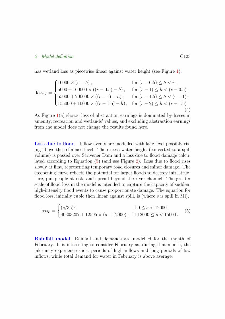
2 Model definition C123

has wetland loss as piecewise linear against water height (see Figure 1):

lossW =

10000× (r − h) , for (r − 0.5) ≤ h < r ,

5000 + 100000× ((r − 0.5)− h) , for (r − 1) ≤ h < (r − 0.5) ,

55000 + 200000× ((r − 1)− h) , for (r − 1.5) ≤ h < (r − 1) ,

155000 + 10000× ((r − 1.5)− h) , for (r − 2) ≤ h < (r − 1.5) .

(4)As Figure 1(a) shows, loss of abstraction earnings is dominated by losses inamenity, recreation and wetlands’ values, and excluding abstraction earningsfrom the model does not change the results found here.

Loss due to flood Inflow events are modelled with lake level possibly ris-ing above the reference level. The excess water height (converted to a spillvolume) is passed over Scrivener Dam and a loss due to flood damage calcu-lated according to Equation (5) (and see Figure 2). Loss due to flood risesslowly at first, representing temporary road closures and minor damage. Thesteepening curve reflects the potential for larger floods to destroy infrastruc-ture, put people at risk, and spread beyond the river channel. The greaterscale of flood loss in the model is intended to capture the capacity of sudden,high-intensity flood events to cause proportionate damage. The equation forflood loss, initially cubic then linear against spill, is (where s is spill in Ml),

lossF =

(s/35)3 , if 0 ≤ s < 12000 ,

40303207 + 12595× (s− 12000) , if 12000 ≤ s < 15000 .(5)

Rainfall model Rainfall and demands are modelled for the month ofFebruary. It is interesting to consider February as, during that month, thelake may experience short periods of high inflows and long periods of lowinflows, while total demand for water in February is above average.

2 Model definition C124

0 1 2 3 4 5 6 7 8 9 100

1

2

3

4

5

6

7

8

9

10

spill (GL)

loss

($00

0,00

0)

Figure 2: Daily loss from downstream flooding against spill; spill in gigal-itres, loss in $millions. A spill of 5 Gl is equivalent to a drawdown of 0.6m.

2 Model definition C125

The rainfall model was developed from daily February rainfall data froma 129 year record. For a given day, rainfall may be zero or strictly posi-tive, according to the proportion of wet and dry (0.7818) days in the record.From that random starting point, a sequence of wet and dry days is gener-ated by a two state Markov chain whose parameters were empirically esti-mated. The wet to dry and dry to wet transition probabilities are 0.4214and 0.1357, respectively. For wet days, rainfall (in mm) is represented bya non-negative random variable, generated by sampling from a truncatedGamma(0.68, 13.35) probability distribution. The Gamma probability den-sity function is

p(y, α, β) =1

βαΓ(α)yα−1 exp−y/β for y, α, β > 0 .

The distribution was fitted to the above-mentioned data (see Figure 3). Wearbitrarily truncate the maximum daily rainfall that could be generated bythe model at 134mm, approximately twice the historical maximum.

Water balance equation The water height of the lake for a given day isthe sum of the previous day’s water level plus stochastic and deterministicinflows, minus evaporation loss, demand and any spill or releases for envi-ronmental flow. Deterministic inflow is from an upstream sewage treatmentplant and evaporation is treated as a constant rate (7.3mm per day) for drydays. We ignore groundwater inflows and seepage losses as little informationon these is available, and they are thought to not make a major contributionto the water balance. Let h(t) be height on day t, i(t) be inflow, d(h(t)) bethe abstraction amount, e be the evaporation rate and f(h(t)) be a releasemade for environmental flow. The water balance equation is

h(t) = h(t− 1) + ki(t)− ks(h(t))− kd(h(t))IA(t)− eIA(t)

− kf(h(t))int

1− t

7+ int

(t

7

)−m(h(t))IB(t) . (6)

We set deterministic inflow at 10Ml per day, stochastic inflow is generatedby the rainfall model with rainfall (in mm) multiplied by 111.3 to obtain

2 Model definition C126

rainfall (mm)

Dens

ity

0 20 40 60 80

0.00

0.05

0.10

0.15

0.20

Figure 3: February rainfall and fitted density.

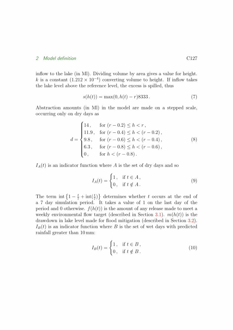
2 Model definition C127

inflow to the lake (in Ml). Dividing volume by area gives a value for height.k is a constant (1.212 × 10−4) converting volume to height. If inflow takesthe lake level above the reference level, the excess is spilled, thus

s(h(t)) = max(0, h(t)− r)8333 . (7)

Abstraction amounts (in Ml) in the model are made on a stepped scale,occurring only on dry days as

d =

14 , for (r − 0.2) ≤ h < r ,

11.9 , for (r − 0.4) ≤ h < (r − 0.2) ,

9.8 , for (r − 0.6) ≤ h < (r − 0.4) ,

6.3 , for (r − 0.8) ≤ h < (r − 0.6) ,

0 , for h < (r − 0.8) .

(8)

IA(t) is an indicator function where A is the set of dry days and so

IA(t) =

1 , if t ∈ A ,

0 , if t /∈ A .(9)

The term int1− t

7+ int( t

7)

determines whether t occurs at the end ofa 7 day simulation period. It takes a value of 1 on the last day of theperiod and 0 otherwise. f(h(t)) is the amount of any release made to meet aweekly environmental flow target (described in Section 3.1). m(h(t)) is thedrawdown in lake level made for flood mitigation (described in Section 3.2).IB(t) is an indicator function where B is the set of wet days with predictedrainfall greater than 10 mm:

IB(t) =

1 , if t ∈ B ,

0 , if t /∈ B .(10)

2 Model definition C128

2.2 Calculation of VaR and CVaR

Let x ∈ X ⊂ Rn be a decision vector, and y ∈ Y ⊂ Rm be a vector represent-ing the values of a contingent variable influencing the loss. Let z = f(x, y)be a function that describes the loss generated by x and y. var and cvarare associated with a particular confidence level, α ∈ (0, 1) . The varα ofthe loss associated with a decision x is defined as

varα(x) = minz | G(x, z) ≥ α , (11)

where G(x, z) is the cumulative density function for loss associated withdecision x. The cvarα of the loss associated with a decision x is defined [7]as

cvarα(x) = Ez | G(x, z) ≥ α , (12)

where E denotes the expectation operator. Figure 4 illustrates var and cvarfor an empirical distribution of loss.

Generating the loss distribution Our decision variable is drawdown ofwater height below the reference level and we consider a range from 0 to 1min 0.05m increments. Loss is calculated on a daily basis in dollar unitsusing Equations (1)–(5). Daily loss is summed to obtain a monthly total andcomputer simulation of 7000 months generates an empirical monthly lossdistribution, G(x, z). Such a distribution is found for a range of values of thedecision variable, x. We set α = 0.90 . We define env to be the mean valueof the monthly loss distribution. In this paper var and env are found as theappropriate quantiles of the loss distribution. cvar is found by numericalcalculation according to the definition in Equation (12).

We are able to generate separate distributions for loss due to low lake lev-els (comprising loss of abstraction, amenity, recreation and wetlands values)and one for high lake levels (loss due to flood). These combine to give thetotal loss distribution. Risk measures are calculated for each of these distri-butions. We define total var (tvar) as the var value calculated from the

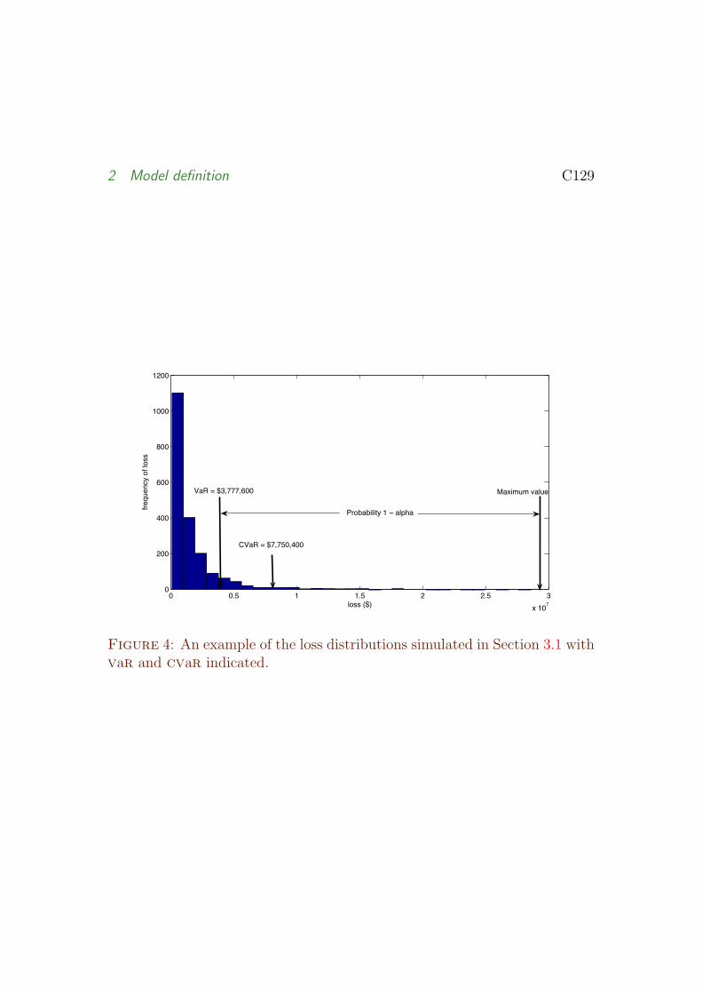
2 Model definition C129

! !"# $ $"# % %"# &'($!)

!

%!!

*!!

+!!

,!!

$!!!

$%!!

-.//(012

34567589:(.3(-.//

;<=(>(1&?)))?+!!

@;<=(>(1)?)#!?*!!

A<'BC7C(D<-75

E4.F<FB-BG:($(!(<-HI<

Figure 4: An example of the loss distributions simulated in Section 3.1 withvar and cvar indicated.

2 Model definition C130

total loss distribution. We define lower cvar (lcvar), upper cvar (ucvar)and total cvar (tcvar) as the cvar value calculated from the distributionsfor loss due to low lake levels, loss due to high lake levels and the combinedloss distribution, respectively. These values are not generally additive, andtcvar can not exceed the sum of lcvar and ucvar. The minimum valuefor tcvar (across the range of values of the decision variable) does not gen-erally coincide with the minimum value for lcvar or that for ucvar. Inmanaging water height primarily to minimise the risk of large losses due toflooding, for example, it may be useful to minimise ucvar against drawdownof water height in order to determine optimal management rules.

3 Simulation results

3.1 Decide minimal water level for release ofenvironmental flows

We set a target for weekly environmental baseflow. Inflows from rainfallcontribute toward meeting the target (or may exceed it). Releases fromthe lake could be made to supplement rainfall and make up any shortfallin environmental flow. We include a penalty, proportional to any shortfall,in the model and find the minimum value of tcvar against our decisionvariable. Thus, a minimum water height could be specified beyond whicha release for environmental flows is not made. Letting c be the penaltyamount, g be the environmental flow target and u be accumulated spill overthe period, our penalty function is

c = 100000× (g − u)

g. (13)

The model tracks spill over a 7 day period and makes supplementary releasesto meet the environmental flow target if there is sufficient water height in

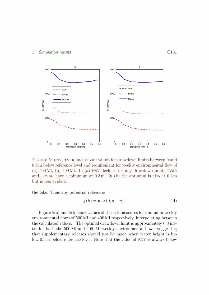
3 Simulation results C131

0 0.1 0.2 0.3 0.4 0.5 0.60

3000

6000

9000a

drawdown limit (m)

loss

($00

0)

ENV

TVaR

TCVaR

0 0.1 0.2 0.3 0.4 0.5 0.60

3000

6000

9000b

drawdown limit (m)

loss

($00

0)

ENV

TVaR

TCVaR

Figure 5: env, tvar and tcvar values for drawdown limits between 0 and0.6m below reference level and requirement for weekly environmental flow of(a) 500Ml, (b) 400Ml. In (a) env declines for any drawdown limit; tvarand tcvar have a minimum at 0.3 m. In (b) the optimum is also at 0.3mbut is less evident.

the lake. Thus any potential release is

f(h) = max(0, g − u) . (14)

Figure 5(a) and 5(b) show values of the risk measures for minimum weeklyenvironmental flows of 500Ml and 400Ml respectively, interpolating betweenthe calculated values. The optimal drawdown limit is approximately 0.3 me-tre for both the 500Ml and 400 Ml weekly environmental flows, suggestingthat supplementary releases should not be made when water height is be-low 0.3m below reference level. Note that the value of env is always below

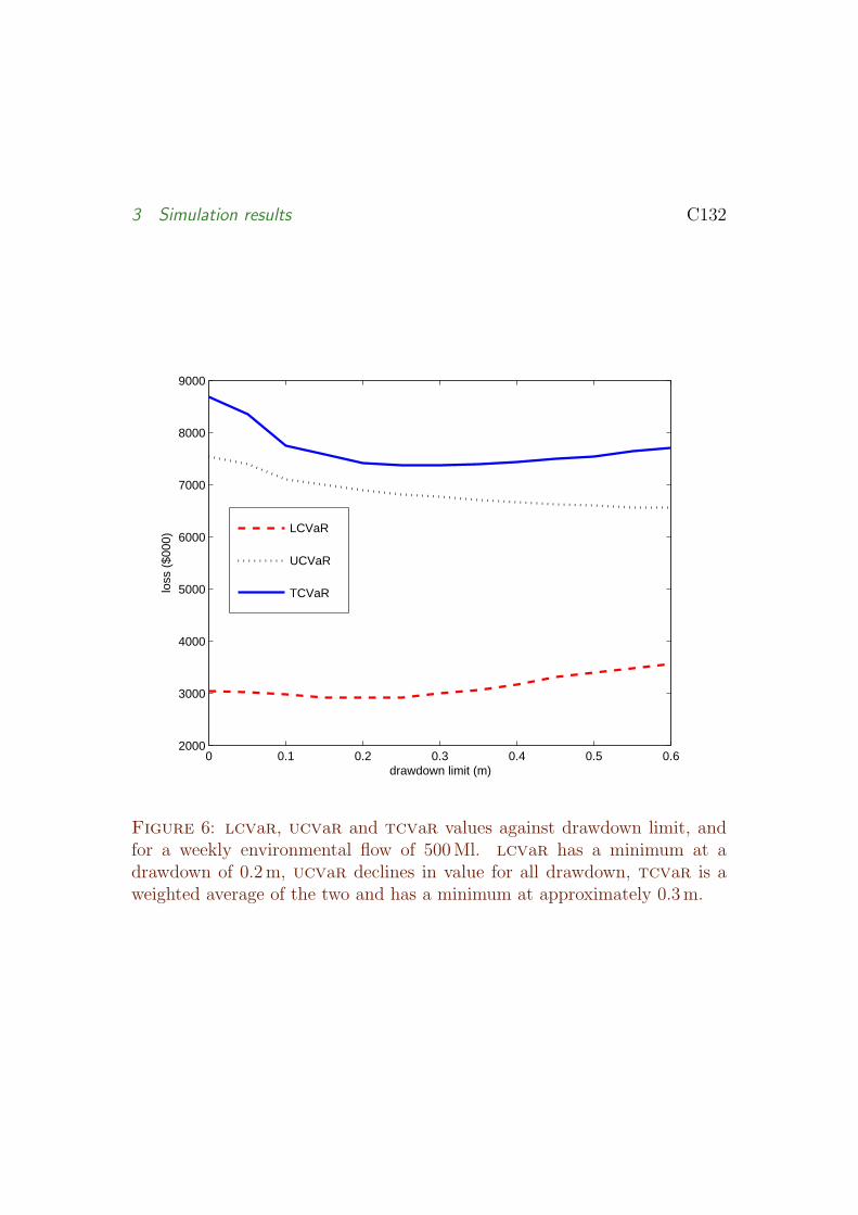
3 Simulation results C132

0 0.1 0.2 0.3 0.4 0.5 0.62000

3000

4000

5000

6000

7000

8000

9000

drawdown limit (m)

loss

($00

0)

LCVaR

UCVaR

TCVaR

Figure 6: lcvar, ucvar and tcvar values against drawdown limit, andfor a weekly environmental flow of 500Ml. lcvar has a minimum at adrawdown of 0.2m, ucvar declines in value for all drawdown, tcvar is aweighted average of the two and has a minimum at approximately 0.3 m.

3 Simulation results C133

that of the two risk measures and that var is similarly always below cvar.cvar is more sensitive to large losses in the tail than var and so is a betterindicator of risk if managers wish to avoid such loss.

Figure 6 shows that lcvar attains a minimum at approximately 0.23mand tcvar at approximately 0.3m. If it was decided that achieving environ-mental flow goals was of overriding importance and we minimise lcvar, weobtain a value of $2915, compared to a value of $7365 for tcvar. Note thatucvar is monotone on this interval, indicating that flood damage is reducedif lake level is drawn down to intercept large flows.

We noticed a trend for the shape of the risk measures to be monotonic. Toobtain minima, the problems had to be balanced between the two competingobjectives. When more weight is placed on the value of having the lake atits reference level, model output indicates that it should never be drawndown. If the weight is on environmental flow goals, the model indicates thatmanagers should always make releases. Thus the model is sensitive to theassumptions made in the loss schedules in Section 2.1.

3.2 Optimal drawdown for flood mitigation

Lake Burley Griffin has a limited capacity to store runoff from rainfall events.If early drawdown of water is made, inflow following rainfall can be antici-pated to refill the lake (with the benefits mentioned in Section 1). However,the conflicting demands of flood mitigation, maintenance of lake referencelevel and river health issues suggest we test for an optimal drawdown valueto minimise loss from the competing objectives. If we had reliable forecaststhat rain would exceed 10 mm in a day but no further information, optimumdraw down is 0.2m below reference level. (See Figure 7). The losses in Fig-ure 7 all assume that a drawdown may be made, provided water height is nolower than 0.3 m below reference level, to meet a weekly environmental flowtarget of 500Ml. It is possible that optimum drawdown for flood mitiga-

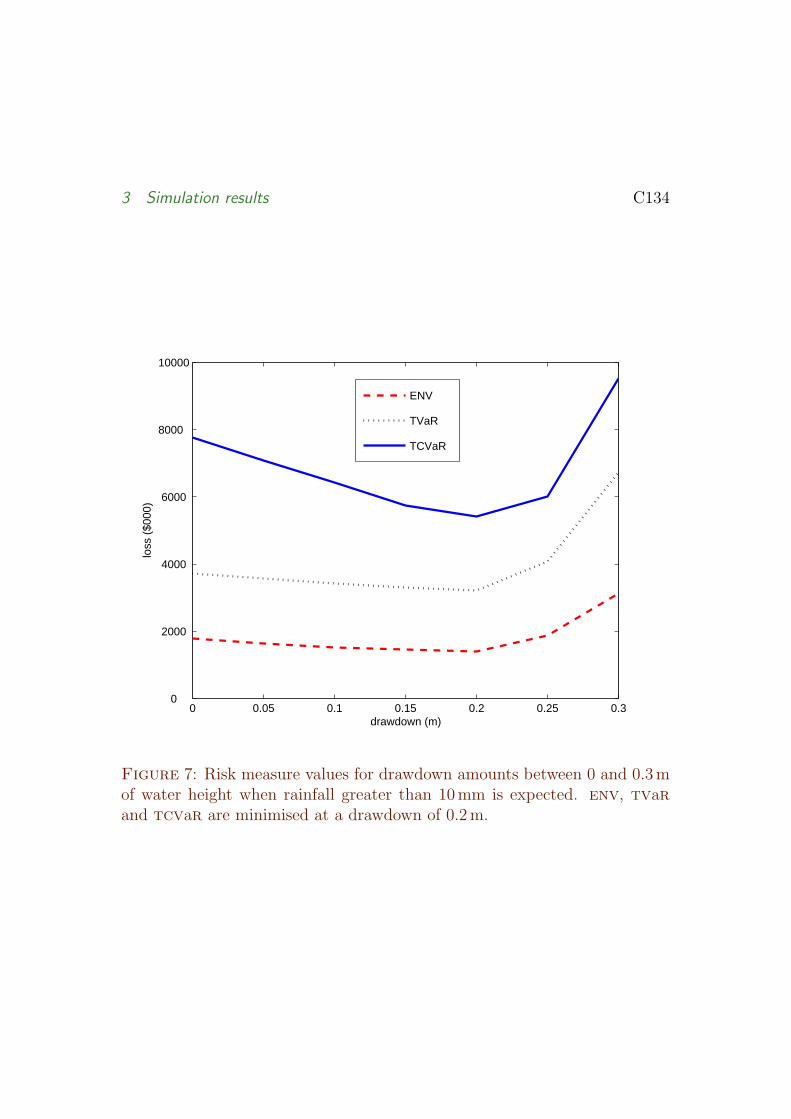
3 Simulation results C134

0 0.05 0.1 0.15 0.2 0.25 0.30

2000

4000

6000

8000

10000

drawdown (m)

loss

($00

0)

ENV

TVaR

TCVaR

Figure 7: Risk measure values for drawdown amounts between 0 and 0.3mof water height when rainfall greater than 10mm is expected. env, tvarand tcvar are minimised at a drawdown of 0.2m.

3 Simulation results C135

tion may depend on the allowable drawdown for environmental flows. Thisrequires further investigation.

4 Conclusion

The model described in this paper was created to assess and demonstratethe potential of using cvar as a tool in developing rules for the optimalmanagement of water height of a lake. Parameter fitting required the settingof values against the degradation of Lake Burley Griffin’s attributes. Themodel found an optimal drawdown of water height for dam releases to meetenvironmental flow targets. Furthermore, it identified an optimum drawdownbefore significant rainfall events to minimise flood losses. We note that, inthe latter scenario, current management strategy is to draw down the lakein these circumstances.

The model is based on Lake Burley Griffin but the methodology could beapplied to similar issues at other reservoirs. To do so requires the assigning ofmonetary values to the water in the reservoir under the range of managementoptions being considered. The relative magnitude placed on the values ofcompeting objectives may be important in model output. An extension ofthe present model is sensitivity testing of our loss distribution parameters.

The values of model parameters and loss distributions assumed here arefor model calculations only. While values for parameters are chosen to rep-resent the real situation, they are assumed values. They should not be takenas real values for any other purposes.

Acknowledgments: We thank the Australian Research Council for sup-porting this research under grant number DP0559399.

4 Conclusion C136

References

[1] National Capital Authority. Lake Burley Griffin Abstraction Plan 2005.National Capital Authority, 2005.http://www.nationalcapital.gov.au/corporate/publications/.C120

[2] R. Ayre, W. Shallcross, and T. Sritharan. Flood management of LakeBurley Griffin. In B. C. Phillips, editor, Proceedings of the 29thHydrology and Water Resources Symposium. Institute of EngineersAustralia, 2005. C118

[3] R. Dahlgren, C. Liu, and J. Lawarree. Risk assessment in energytrading. IEEE Transactions On Power Systems, 18:503–511, 2003.http://dx.doi.org/10.1109/TPWRS.2003.810685 C119

[4] C. Harman and M. Stewardson. Optimising dam release rules to meetenvironmental flow targets. River Research And Applications,21:113–129, 2005. http://dx.doi.org/10.1002/rra.836 C119

[5] M. Jenkins, J. Lund, and R. Howitt. Using economic loss functions tovalue urban water scarcity in California. Journal of the AmericanWater Works Association, 95:58–70, 2003. C119

[6] L. Pruzzo, R. Cantet, and C. Fioretti. Risk-adjusted expected return forselection decisions. Journal of Animal Science, 81:2984–2988, 2003.http://jas.fass.org/cgi/content/full/81/12/2984 C119

[7] R. Rockafellar and S. Uryasev. Conditional value-at-risk for general lossdistributions. Journal of Banking and Finance, 26:1443–1471, 2002.http://dx.doi.org/10.1016/S0378-4266(02)00271-6 C128

102

Reducing the Vulnerability of Societies to Water Related Risks at the Basin Scale (Proceedings of the third International Symposium on Integrated Water Resources Management, Bochum, Germany, September 2006). IAHS Publ. 317, 2007.

297

Conditional Value-at-Risk analysis of flooding in the Lower Mekong Basin BRIAN WEBBY1, PETER ADAMSON1, JOHN BOLAND2, PHIL HOWLETT2 & ANDREW METCALFE1

1 The University of Adelaide, Adelaide, South Australia 5005, Australia roger.webby@adelaide.edu.au

2 Centre for Industrial and Applied Mathematics, The University of South Australia, Mawson Lakes, Adelaide, South Australia 5095, Australia

ANZIAM J. 48 (CTAC2006) pp.C885–C898, 2008 C885

Stochastic linear programming andConditional Value-at-Risk for water resources

management

R. B. Webby1 J. Boland2 P. G. Howlett3

A. V. Metcalfe4

(Received 1 September 2006; revised 16 January 2008)

Abstract

A mathematical analysis is presented for decision support for man-aging water resources in a water-limited environment. The watersources include rainfall, either direct or that held in reservoirs, shal-low aquifers, river water withdrawal entitlements, and recycled water.Water from each source has its own characteristics of quality andthus suitability for use, quantity, temporal availability, environmentalimpact of use and cost to access. Water availability is modelled by amultivariate probability distribution. Relative values for salinity levelsand nutrient or mineral loads are given and other water characteristicsare summarised by a price for water from each source. We formulate

See http://anziamj.austms.org.au/ojs/index.php/ANZIAMJ/article/view/136for this article, c© Austral. Mathematical Soc. 2008. Published January 30, 2008. ISSN1446-8735

Contents C886

and solve a stochastic linear program to find the optimal blend ofthe available sources while meeting quality and supply constraints.We apply these techniques to a common water resource managementproblem facing an Australian farmer, that of growing a summer cropusually reliant on irrigation. We compare alternate cropping decisionsbased on their risk of failing to meet supply or quality standards. Ourmeasure of risk is Conditional Value-at-Risk.

Contents

1 Introduction C887

2 Model definition C8882.1 Definition of VaR and CVaR . . . . . . . . . . . . . . . . . C8882.2 Stochastic linear programming . . . . . . . . . . . . . . . . C8892.3 Water characteristics . . . . . . . . . . . . . . . . . . . . . C891

3 Simulation results C8923.1 Feasibility of supply . . . . . . . . . . . . . . . . . . . . . . C8923.2 Water requirement of crop . . . . . . . . . . . . . . . . . . C8933.3 CVaR and expected return . . . . . . . . . . . . . . . . . . C8943.4 Value of entitlement . . . . . . . . . . . . . . . . . . . . . C8953.5 Model extension . . . . . . . . . . . . . . . . . . . . . . . . C895

4 Conclusion C896

References C897

1 Introduction C887

1 Introduction

To illustrate the use of Conditional Value-at-Risk (cvar) as a decision sup-port tool for water resource managers, we present an application focussingon the irrigation requirements of a summer crop in a water limited environ-ment. In this situation, water may be available from a number of sourcessuch as rainfall, shallow aquifer groundwater, an entitlement to withdrawriver water, and tailwater, that is, water collected from previous crop irriga-tion operations and recycled. This is a study to explore what questions canbe asked using this approach and we present a simple model. The results aremore to support intuition than to make reliable decisions.

Yamout and El-Fadel [3] formulated a linear program for a domesticwater supply problem for Greater Beirut. Water supplies were determin-istic and they included socio-environmental practices as constraints. Linearand non-linear programming algorithms have been used in coal blending forpower generation, treating sources of coal as having known quality and quan-tity characteristics [1, e.g.]. Here we allow water from some sources to bestochastic in availability. We solve a linear program to minimise the costof providing water which must meet quantity and quality constraints. Weevaluate alternate decisions in terms of the linear program solutions and thecvar values calculated from a distribution for minimum cost built up fromsampling instances of the stochastic variable. cvar has been applied in cropselection [4], where a maximum value of cvar was included as a constraintin a linear program.

In deciding to grow a summer crop a farmer determines whether sufficientwater is available to bring the crop to harvest, and compares the cost of thatwater and other input costs against the expected return. However, wateris a crucial input to producing a crop and in this stochastic linear programformulation of the decision problem we focus on the frequency of seriouslyadverse events. The information from our solutions could be used to guidefuture practical farm works, and also the level of hedging (crop insurance or

2 Model definition C888

futures products) that might be applied to cover the investment in the crop.

2 Model definition

2.1 Definition of VaR and CVaR

Value-at-Risk (var) is a measure of risk developed in the finance industryfor evaluating the risk exposure of a portfolio of financial instruments such asshares, bonds and derivatives. var is defined as the maximum loss expectedto be incurred over a given time horizon at a specified probability level.Mathematically, let x ∈ X ⊂ Rn be a decision vector and y ∈ Y ⊂ Rm bea vector representing the values of a contingent variable influencing the loss.Let z = f(x, y) be a function that describes the loss generated by x and y. Atprobability level α ∈ (0, 1), the varα of the loss associated with a decision xis defined as [2]

varα(x) = infz | G(x, z) ≥ α , (1)

where G(x, z) is the cumulative density function for loss associated withdecision x.

var gives the value of the specified quantile of the distribution but doesnot give any information about the upper tail beyond that value. That is,var describes the frequency of a sizable loss but not the likely severity ofsuch a loss. cvar does contain information about losses in the upper tail.cvar is the expected loss, given that a loss greater than or equal to thethreshold var occurs. The cvarα of the loss associated with a decision x isdefined as [2]

cvarα(x) = Ez | G(x, z) ≥ α , (2)

where E denotes the expectation operator.

In this article we generate a cost, rather than loss, distribution throughsimulation of a mathematical model of the system. var is then found as the

2 Model definition C889

0 0.5 1 1.5 2 2.5 3 3.5

x 105

0

800

1600

2400

cost ($)

freq

uenc

y VaR = $162,000 Maximumvalue

Probability 1 − α

CVaR = $180,940

Figure 1: An example of the cost distributions simulated in Section 3 withvar and cvar indicated.

αth proportional value of the ordered distribution, and cvar as the meanof the values equal to or beyond var. Figure 1 shows var and cvar valuesfor an empirical cost distribution generated by our model for Section 3. Themean cost is $96,095 and although most of the simulated costs are less than$200,000, there is a positive probability of experiencing costs of 31

2times

the average. For this distribution var is $162,000 and cvar approximately$181,000. cvar will always be greater than or equal to var.

2.2 Stochastic linear programming

Linear programming involves problems of the form

min cTx ,

subject to Ax ≤ b ,

l ≤ x ≤ u ,

where cTx is a cost function, l is a lower bound and u an upper bound for x.The cost function is minimised subject to constraints which may be equalityor inequality constraints. Stochastic linear programming allows for some

2 Model definition C890

elements of the constraint equations to be stochastic. In this applicationsome elements of b are stochastic.

One approach to solving stochastic linear programs is to take particu-lar values for the stochastic variables and solve the resulting deterministicproblem. Values typically chosen are the expected value of the variable, itsexpected value plus and minus one or two standard deviations, or simplya spread of possible values of the variable. Another approach is to sam-ple values from the distributions of the random variables and again solve adeterministic program. This method is particularly suited where there arecorrelations between the stochastic variables. Our approach, this latter one,involved specifying a multivariate normal distribution for the availability ofrainfall and groundwater, allowing us to incorporate correlation between therandom variables. Methods for generating samples for the multivariate nor-mal are readily available but other distributions could be used. A copula orthe empirical Gibbs sampler could also be used to generate multivariate datafrom arbitrary distributions. After sampling values from the input distribu-tions, we use linear programming to find the optimal blend of water from thefour sources to obtain the lowest cost for producing the crop. The programis run multiple times to build up an empirical distribution for the minimumcost and calculate cvar values for the distribution.

We set xj, j = 1, . . . , J , to represent the amount of water taken from eachsource j. The cost of the water is cj, and the amount of water available fromeach source in a given summer is aj. Each source has a particular salinityconcentration, sj, and mineral or nutrient load, mj, and we set maximumlevels for these in the blended water of S and M respectively. We consideran individual crop with a water requirement for full potential productivityacross a crop area of H hectare of X Ml. Expressed as a linear program, thewater blending problem is

min∑j

cjxj ,

such that xj ≤ aj ,

2 Model definition C891

∑j

sjxj

/ ∑j

xj ≤ S ,

∑j

mjxj

/ ∑j

xj ≤M ,∑j

xj ≥ X ,

xj ≥ 0 for j = 1, . . . , n .

2.3 Water characteristics

We characterize the various water supplies as shown in Table 1. The salinityvalues are typical values encountered in inland cropping areas of Australiaand here are fixed as a summer average, although they could also be madestochastic. For example, bore and river water may increase non-linearlyin salinity throughout a summer. The mineral or nutrient loads are typicalrelative values for each source, and could represent sodicity levels in soil wateror nitrate levels in recycled water. We use a bivariate normal distributionto represent the amounts of rainfall and groundwater available and modelthem as being correlated with a coefficient of 0.7. Cost per Ml of water isintended to represent the relative cost of accessing water from the respectivesources. It then would include pumping, storage and application costs, andassumes the same application method is used for each crop, as well as coststo represent the environmental cost of using water from a given source. Weare not certain of the accuracy of some of our parameters so have not carriedout sensitivity tests on them.

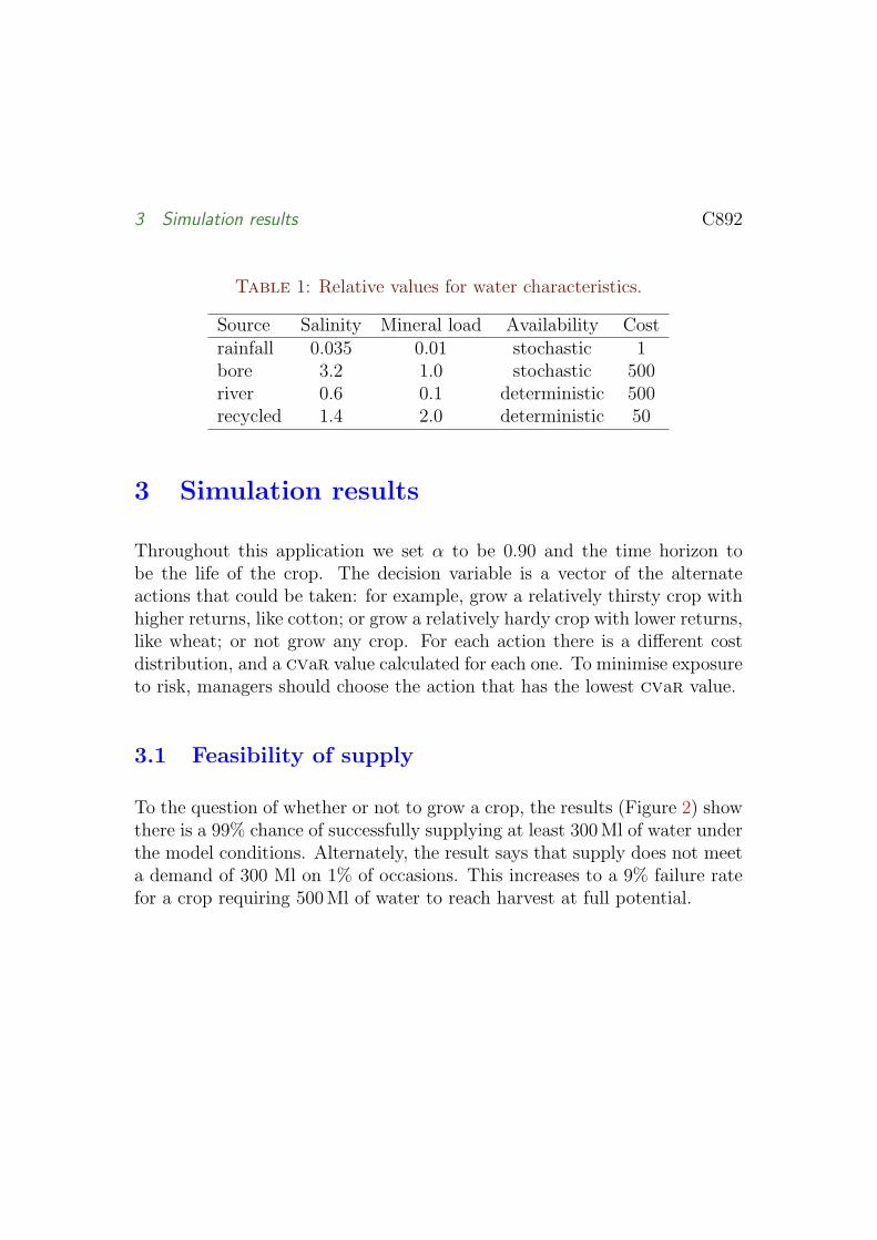
3 Simulation results C892

Table 1: Relative values for water characteristics.

Source Salinity Mineral load Availability Costrainfall 0.035 0.01 stochastic 1bore 3.2 1.0 stochastic 500river 0.6 0.1 deterministic 500recycled 1.4 2.0 deterministic 50

3 Simulation results

Throughout this application we set α to be 0.90 and the time horizon tobe the life of the crop. The decision variable is a vector of the alternateactions that could be taken: for example, grow a relatively thirsty crop withhigher returns, like cotton; or grow a relatively hardy crop with lower returns,like wheat; or not grow any crop. For each action there is a different costdistribution, and a cvar value calculated for each one. To minimise exposureto risk, managers should choose the action that has the lowest cvar value.

3.1 Feasibility of supply

To the question of whether or not to grow a crop, the results (Figure 2) showthere is a 99% chance of successfully supplying at least 300 Ml of water underthe model conditions. Alternately, the result says that supply does not meeta demand of 300 Ml on 1% of occasions. This increases to a 9% failure ratefor a crop requiring 500 Ml of water to reach harvest at full potential.

3 Simulation results C893

0.9

0.92

0.94

0.96

0.98

1

0 100 200 300 400 500 600

water required (Ml)

succ

ess

rate

(%

)

Figure 2: Percentage of simulations meeting various crop water require-ments.

3.2 Water requirement of crop

Given that it is decided to grow a crop, should it be a relatively high waterdemanding crop? or a relatively low water demanding one? Expressed an-other way the problem is: given that we are able to grow a range of cropswith specific water requirements for full growth potential, what area of eachcrop should be grown? As Figure 3 shows, the cost distribution of producingthe thirsty crop has high variability and a bias toward higher values, whilethe bulk of the simulated costs for a hardy crop are low and the distributionis exponential in nature. The cvar0.90 value for the more thirsty crop ishigher ($239,459 as against $79,377) as intuition would suggest. In effect,the cvar values for both crops and particularly the thirsty crop are higherthan stated as we have excluded the infeasible solutions from their calcula-tion. Costs cannot be found for the infeasible solutions; however, they wouldbe at least as great as the highest costs for feasible solutions. They could be

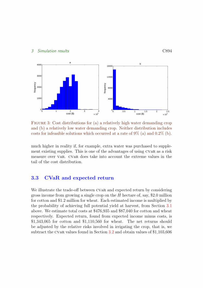
3 Simulation results C894

0 1 2 3 4x 105

0

1000

2000

3000

4000

cost ($)

frequ

ency

a

0 0.5 1 1.5 2 2.5x 105

0

4000

8000

12000

16000

cost ($)

frequ

ency

b

Figure 3: Cost distributions for (a) a relatively high water demanding cropand (b) a relatively low water demanding crop. Neither distribution includescosts for infeasible solutions which occurred at a rate of 9% (a) and 0.2% (b).

much higher in reality if, for example, extra water was purchased to supple-ment existing supplies. This is one of the advantages of using cvar as a riskmeasure over var. cvar does take into account the extreme values in thetail of the cost distribution.

3.3 CVaR and expected return

We illustrate the trade-off between cvar and expected return by consideringgross income from growing a single crop on the H hectare of, say, $2.0 millionfor cotton and $1.2 million for wheat. Each estimated income is multiplied bythe probability of achieving full potential yield at harvest, from Section 3.1above. We estimate total costs at $476,935 and $87,040 for cotton and wheatrespectively. Expected return, found from expected income minus costs, is$1,343,065 for cotton and $1,110,560 for wheat. The net returns shouldbe adjusted by the relative risks involved in irrigating the crop, that is, wesubtract the cvar values found in Section 3.2 and obtain values of $1,103,606

3 Simulation results C895

0 1 2 3 4x 105

0

2000

4000

6000

cost ($)

frequ

ency

a

0 1 2 3 4x 105

0

2000

4000

6000

cost ($)

frequ

ency

b

Figure 4: Cost distributions for (a) river water valued at a nominal rateand (b) river water valued at two times the nominal rate.

and $1,031,183, for a financial advantage of cotton over wheat of $72,423.

3.4 Value of entitlement

River water entitlements may become more valuable if water can be sold toother users. For this analysis, we double the cost of river water to representthe opportunity cost of not selling the water. Growing a crop that requires500 Ml of water (Figure 4), the two cost distributions have a similar shapebut are shifted along the horizontal axis. There is about a 75% increase inthe cvar value for the higher valued water.

3.5 Model extension

The model described here can be easily extended to consider growing of arange of crops in the one season. The farmer would grow k crops, k =1, . . . , K , with area hk under each crop. The decision variable is the relative

4 Conclusion C896

proportion of the total cropping area to allocate between crops that requirediffering amounts of water. Then our linear program has added constraintshk ≥ 0 and

∑k hk ≤ H for k = 1, . . . , K . The constraint that supply from

all sources,∑

j xj, at least equals demand, X, is required for a single cropand for a mixture of crops. It is possible to implement constraints repre-senting individual salinity (or mineral load) tolerances for different crops as∑

j

∑k sjxjk/

∑j

∑k xjk ≤ Sk for k = 1, . . . , K . This multiple-crop problem

is not solved here but Liu et al. [4] give a related example.

4 Conclusion

Management of water, on farm and off, is becoming more critical due to theincreasing demand, increasing value and, in some areas, decreasing availabil-ity of the resource. We present a mathematical analysis for a typical farmwater blending problem where water from a variety of sources must meetquantity and quality specifications for crop production. A stochastic linearoptimisation model represents the variability in water availability and croprequirements. Monte Carlo simulation is used to test a range of actions rele-vant to a farming operation and identify the preferred options. We make useof a conservative risk measure, cvar, which reveals the exposure to risk ofpossible rare but devastating events. Our model quantifies the rate at whichsupply fails to meet demand; we generate cost distributions and calculatetheir cvar values. While the application of our model in this article is gen-eral, using values encountered in the Narrabri region, its parameters couldbe specified to match conditions applying to any particular farm property.

Acknowledgements We thank the Australian Research Council for sup-porting this research under grant number DP0559399.

References C897

References

[1] F. J. Vasko, D. D. Newhart, and A. D. Strauss. Coal blending modelsfor optimum cokemaking and blast furnace operation. Journal of theOperational Research Society, 56: 235–243, 2005.doi:10.1057/palgrave.jors.2601846 C887

[2] R. T. Rockafellar, and S. Uryasev. Conditional Value-at-Risk forGeneral Loss Distributions. Journal of Banking and Finance, 26:1443–1471, 2002. doi:10.1016/S0378-4266(02)00271-6 C888

[3] G. Yamout, and M. El-Fadel. An optimisation approach for multi-sectorwater supply management in the Greater Beirut area. Water ResourcesManagement, 19: 791–812, 2005. doi:10.1007/s11269-005-3280-6 C887

[4] J. Liu, C. Men, V. E. Cabrera, S. Uryasev, and C. W. Fraisse. CVaRmodel for optimizing crop insurance under climate variability. ResearchReport 2006-1, Risk Management and Financial Engineering Lab,University of Florida, 2006.http://www.ise.ufl.edu/uryasev/pubs.html C887, C896

References C898

Author addresses

1. R. B. Webby, School of Mathematical Sciences, University ofAdelaide, Adelaide, Australia.mailto:roger.webby@adelaide.edu.au

2. J. Boland, Centre for Industrial and Applied Mathematics,University of South Australia, Adelaide, Australia.

3. P. G. Howlett, Centre for Industrial and Applied Mathematics,University of South Australia, Adelaide, Australia.

4. A. V. Metcalfe, School of Mathematical Sciences, University ofAdelaide, Adelaide, Australia.

ANZIAM J. 49 (EMAC2007) pp.C184–C199, 2007 C184

Stochastic programming to evaluate renewablepower generation for small-scale desalination

R. B. Webby1 J. Boland2 A. V. Metcalfe3

(Received 26 July 2007; revised 8 November 2007)

Abstract

Due in part to an increasing population and climatic change, freshwater demand is rapidly outpacing fresh water supply. In Australiadesalination plants are already used to obtain fresh water from brack-ish water and seawater, but they have high energy requirements. Solarcollectors could provide power, but solar irradiance is variable and de-salination plants work most efficiently with constant power. We modela system of photovoltaic arrays and storage batteries. Daily solar in-tensity and water demand are stochastic. A stochastic linear programfinds the optimal blend of water from available sources—groundwater,desalination and stormwater—to meet daily demand. The optimal useof a given size of solar irradiance collection system is found by stochas-tic dynamic programming. Long term net benefits are obtained as afunction of the system size.

See http://anziamj.austms.org.au/ojs/index.php/ANZIAMJ/article/view/320for this article, c© Austral. Mathematical Soc. 2007. Published November 13, 2007. ISSN1446-8735

Contents C185

Contents

1 Introduction C185

2 Stochastic dynamic program C1862.1 Defining the state space . . . . . . . . . . . . . . . . . . . C1872.2 Solar irradiance input to the system . . . . . . . . . . . . . C1912.3 Optimal policies . . . . . . . . . . . . . . . . . . . . . . . . C191

3 Stochastic linear program C194

4 Conclusions C196

References C197

1 Introduction

People living in arid and semi-arid Australia frequently face a shortage ofpotable water. But remote communities, national parks, stations and islandsoften have access to saline groundwater or sea water, along with abundant so-lar energy. These locations are generally not connected to the electricity gridand researchers are investigating autonomous systems of desalination mod-ules powered by renewable energy for such locations. Investigations includepilot projects in Australia [6] and the Mediterranean region [1], and math-ematical models of renewable powered desalination plants to simulate theiroperation [4, 5]. Both practical and mathematical models aim to provideguidance for system sizing and efficient operational strategies. The poten-tially useful technique of stochastic programming has been used to analyseboth short term and long term planning issues in the allied arena of thederegulated electricity market [3]. However, it has not been used in decisionmaking for renewable power generation for small scale desalination systems.

2 Stochastic dynamic program C186

We describe a mathematical model of a solar energy powered, reverseosmosis desalination plant using stochastic programming to assess systemsizing, operating rules and longer term objectives of water production. Theplant comprises a photovoltaic (pv) array connected to an energy storagesystem of batteries and to two desalination modules that can be run inde-pendently of each other. A stochastic dynamic programming (sdp) algorithmfinds the optimal policy for the allocation of energy flows from the pv arraywhile meeting typical plant operating conditions. Results from the sdp arean input to a stochastic linear program (slp) which matches water demandto supply at lowest cost while meeting availability and salinity constraints.

2 Stochastic dynamic program

The sdp algorithm uses transition matrices whose entries, pij(k), which de-pend on a decision k, are the probability of moving between states of the statespace, and a reward matrix whose entries, rij(k), are the value obtained bymaking a particular transition under decision k. Let i ∈ 1, 2, . . . ,m repre-sent the states of the system. For our model, m = 18 . Let t ∈ 0, 1, . . . , Tbe discrete one hour time periods. The policy iteration procedure is imple-mented in two parts: value determination and policy improvement [2]. For agiven policy, total expected earnings over the remaining time steps at time tdepends on the state, i, at time t, and is written vt(i). For a given policy,total expected earnings is calculated recursively as

vt(i) =∑

all states j

pij[rij + vt+1(j)] , for j = 1, . . . ,m . (1)

For large t,vt(i) = g + vt+1(i) ,

2 Stochastic dynamic program C187

where g is the expected return per period. Substituting into (1) gives the setof equations making up the value determination step:

g + v(i) =∑

j

pijrij +∑

j

pijv(j) , i = 1, . . . ,m . (2)

These equations are solved for g and v(2) up to v(m) with v(1) being arbi-trarily set to 0 in order to obtain a solution for the under determined system.The policy improvement step maximises for all states i∑

j

p′ij(k)r′ij(k) +∑

j

p′ij(k)v(j) . (3)

The algorithm starts with an arbitrary policy and continues until the policiesproduced on two successive iterations are identical.

Model assumptions

We assume that the process of desalination requires a desalination moduleto be run for two hours to produce a unit quantity of desalinated water, andthat a module run for one hour produces no potable water. This assumptionrecognises that for efficient operation of reverse osmosis modules, the waterpressure and the brine to feedwater ratio in the modules must be carefullyregulated to ensure the quality of the water produced, to manage and disposeof the brine stream, and to minimise scaling of membrane surfaces. Weassume that a module uses one unit of energy per hour when running.

2.1 Defining the state space

The time step of the model is one hour, a period of similar scale to thedesalination process, avoiding excessive start/stop operations but allowingthe system to take advantage of favourable conditions. The time scale could

2 Stochastic dynamic program C188

be altered if there is evidence that this is necessary. We specify discretestates for each desalination module of 0, 1, 2, where state ’0’ represents themodule being unused, state ’1’ represents the module having completed thefirst hour of the desalination process, and state ’2’ represents the modulehaving completed the second hour of the desalination process. We specifydiscrete states for the storage level of the battery assemblage and assumethe assemblage has a storage capacity of B, so that b ∈ 0, B representsthe number of recoverable units of energy held in storage. For the initialformulation of the problem we set the states of the battery assemblage tobe 0, 1. Thus storage capacity is one unit and we assume that excessenergy cannot be used in this application.

The state space of the problem is made up of triplets, (m1 m2 b), wherem1 ∈ 0, 1, 2 records the state of module 1, m2 ∈ 0, 1, 2 records the stateof module 2, and b ∈ 0, 1 records the state of the battery storage. Thereare three possible states for each desalination module and two for the batteryassemblage, giving 18 combinations. The state space of the problem, in theorder arbitrarily chosen here, is

(000), (010), (020), (001), (011), (021), (100), (110), (120),

(101), (111), (121), (200), (210), (220), (201), (211), (221).

We consider three decisions, k ∈ 0, 1, 2 (Figure 1): 0, run no desalina-tion modules; 1, run one desalination module only; 2, run both desalinationmodules.

A decision is made at hourly intervals at the beginning of a time period inthe knowledge of the state of the system and the probability of energy inflowsfor the next hour. The decision is made for the time period immediatelyfollowing and energy flows during that time period are directed according tothe decision.

Energy inflows from the pv array are stochastic and we model inflowamounts to be compatible with the discrete quantities of the state space.

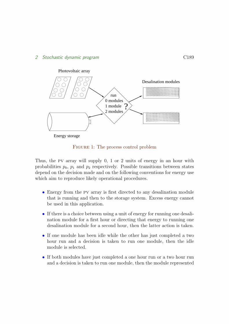
2 Stochastic dynamic program C189

Photovoltaic array

Energy storage

Desalination modules

run

2 modules1 module0 modules

?

Figure 1: The process control problem

Thus, the pv array will supply 0, 1 or 2 units of energy in an hour withprobabilities p0, p1 and p2 respectively. Possible transitions between statesdepend on the decision made and on the following conventions for energy usewhich aim to reproduce likely operational procedures.

• Energy from the pv array is first directed to any desalination modulethat is running and then to the storage system. Excess energy cannotbe used in this application.

• If there is a choice between using a unit of energy for running one desali-nation module for a first hour or directing that energy to running onedesalination module for a second hour, then the latter action is taken.

• If one module has been idle while the other has just completed a twohour run and a decision is taken to run one module, then the idlemodule is selected.

• If both modules have just completed a one hour run or a two hour runand a decision is taken to run one module, then the module represented

2 Stochastic dynamic program C190

by the first element of the state space triplet is selected.

We illustrate the calculation of the entries of the transition matrices.Decision 2 is to run two desalination modules. In state (000), for example,neither module has been in use in this time step and no energy was stored.A decision is taken to run two modules. With probability p0, no energy isavailable from the pv array during the current time step, the desalinationprocess is halted and the system remains in state (000). With probability p1,one unit of energy is obtained through the pv collectors and the system movesfrom state (000) to state (100). With probability p2, the system moves tostate (110).

A cost of r is incurred when a desalination module is run for up to onehour. The cost includes pretreatment of the feedwater such as screeningand filtering, chemical treatment of cations and storage of cleaned feedwater.The cost also includes backflushing and eventual replacement of membranes,disposal of brine and storage of the product. A benefit of r is assigned forcompleting the first hour of desalination. Thus a transition to state (100),say, has a reward of −r + r = 0 . A benefit of 2r is obtained for completingthe second hour of desalination. Thus an eventual transition to state (200),say, has a reward of −r + 2r = r . Any decision taken is implemented at thebeginning of a time step. If a decision is taken to run a module but thereis insufficient energy to complete the run, the cost of running the moduleis incurred without any benefit, thus the reward is −r per module started.The net result of this is that an overall benefit of r accrues if a desalinationmodule completes two hours of running and an overall loss (benefits minuscosts) of r accrues if the module is run and fails to complete one hour or failsto complete two hours.

2 Stochastic dynamic program C191

2.2 Solar irradiance input to the system

We characterise energy levels in the system as being of 0, 1 or 2 units wherean energy level of 0 units is insufficient to run a desalination module for onehour, a level of 1 unit is sufficient energy to run one desalination module forone hour, and a level of 2 units is sufficient to run one desalination modulefor two hours. We use a 38 year data record to characterise energy input tothe pv array and model solar irradiance for January and July—potentiallythe months of greatest and least solar energy. Average hourly direct beamsolar insolation for Adelaide for the period from 6 am to 6 pm in January and8 am to 4 pm in July has a similar distribution of intensity for each hour,and so we aggregated the data to represent a typical hour’s insolation forthese two periods (Figure 2). We set the ranges of solar irradiance thatconstitute 0, 1 or 2 units of energy as: 0 units for solar irradiance between 0and 150 Whm−2; 1 unit for solar irradiance between 150 and 450 Whm−2;and 2 units for solar irradiance between 450 and 1150 Whm−2. Thus theprobabilities of irradiance amounts within the three ranges of direct beamsolar irradiance falling on a dual-tracking pv array are, for January 6 amto 6 pm, 0.15, 0.21 and 0.64 respectively, and, for July 8 am to 4 pm, 0.37,0.30 and 0.33 respectively. We assume that the energy produced by the pvarray is a linear function of solar irradiance but a more detailed model wouldinclude the degradation of array performance at higher temperatures [5].

2.3 Optimal policies

A policy specifies a decision for each state of the system. We write a policy asa vector with the elements of the vector representing the states of the systemin our chosen order and the entries of the vector as the respective decisions.

2 Stochastic dynamic program C192

0 400 800 12000

1200

2400

3600a

Whm!2

frequ

ency

0 400 800 12000

1200

2400

3600b

Whm!2

frequ

ency

Figure 2: Direct beam solar insolation at Adelaide for daylight periods:(a) January, 6 am to 6 pm; and (b) July, 8 am to 4 pm.

July, 8 am–4 pm

sdp analysis gives an optimal policy of

[0 1 0 1 1 1 1 1 1 1 2 1 0 1 0 1 1 1] .

There is one state in which it is optimal to run both modules simultaneously,but, under the optimal policy, the system cannot reach this state. In sum-mary, the operating rules under this policy are: if a desalination module hasjust completed the first hour of the process, run it for the second hour; ifboth modules are available and there is energy in storage, start one module;else, run no modules. Taking this latter decision means, in practical terms,that any incoming energy is used to build up stored energy.

The average, long term, desalinated water production under this policyis 0.31 units per hour. Note that either one or no module is run in any timestep and thus the plant is under utilised.

2 Stochastic dynamic program C193

January, 6 am–6 pm

sdp analysis gives an optimal policy of

[1 1 1 1 2 1 1 2 1 2 2 2 1 1 1 1 2 1] .

The operating rules under this policy are: run at least one desalination mod-ule in any state; run two modules if one of the modules has just completed itsfirst hour of desalination and the system has stored energy, and if both mod-ules have just completed their first hour of desalination but with no energyin storage.

The average, long term, desalinated water production under this policyis 0.70 units per hour. At least one desalination module is run at each timestep and thus the system is utilised more fully under this policy. The hourlydesalinated water production in July is approximately 44% of hourly produc-tion in January. However, due to the longer period of daylight and thus theextended operational time in January, daily desalinated water production inJuly is approximately 30% that of January.

Expanded storage states

During the design phase of a photovoltaic system particular attention is givento deciding on the relative sizes of the solar collector array and an energystorage system. For example, sufficient storage capacity may be providedto run a plant at its average production rate for one to two days withoutexternal energy input. As an extension to our basic model, we expand thestate space by doubling potential storage capacity, so that the states of storedenergy are 0, 1, 2. The state space for the problem is now

(000), (010), (020), (001), (011), (021), (002), (012), (022),

(100), (110), (120), (101), (111), (121), (102), (112), (122),

3 Stochastic linear program C194

(200), (210), (220), (201), (211), (221), (202), (212), (222).

Rewriting transition and reward matrices to follow model assumptionsand conditions as before and conducting sdp analysis gives an optimal policyfor July, 8 am to 4 pm of

[0 0 0 1 1 1 1 2 1 0 0 0 1 1 1 2 2 2 0 0 0 1 1 1 1 2 1] ,

and an optimal policy for January, 6 am to 6 pm is

[0 1 0 1 1 1 2 2 2 1 1 1 1 2 1 2 2 2 0 1 0 1 1 1 2 2 2] .

The average, long term, desalinated water production for July is 0.38 unitsper hour while that for January is 0.72 units per hour. Thus extra energystorage increased water production by 23% during July and by 3% in January.Thus, system sizing is adequate for January but added storage capacity couldincrease water production during July. Note that water demand may be lowerin July.

3 Stochastic linear program

We consider daily household and agricultural demands for water for a smallcommunity in January. Household use includes cooking, drinking and wash-ing while agricultural use includes drinking water for stock and irrigation offood crops. We consider three sources of supply of water: rainfall as stochas-tic; a low salinity source of groundwater as deterministic; and output fromthe desalination plant also as stochastic. The triangular distribution for de-salinated water production is suitable for such a process where the maximum,minimum and most likely values are known. The gamma(49,7) distributionproduces random rainfall that satisfies, on average, one third of demand.Demand is modelled as a bivariate normal distribution for household and

3 Stochastic linear program C195

Table 1: Water characteristics of sources and sinkssource rain ground desalavailability (units) ∼gamma(49,7) up to 9 ∼triang(0,12)salinity (mg/l) 100 1500 500

sink household agriculturaldemand (units) (correlation = 0.6) ∼N(1.5,0.22) ∼N(15,1.22)maximum salinity (mg/l) 500 900

agricultural uses with average agricultural demand ten times that of house-hold demand. These are positively correlated to reflect similar patterns ofdemand from both uses during similar climatic conditions (Table 1).

Let r, g and d represent the sources of rain, ground and desalinatedwater, respectively. Let h and a represent the demand sites of household andagricultural use. Let xij be the amount of water supplied from source i todemand site j and cij be the cost of such supply. We write the quantity ofwater available from source i in a given time step as availi, the demand atsite j as demj, and the salinity conditions of the sources and demand sitesas sali and salj respectively. The linear program is

min∑ij

cij xij,

such that∑

i

xij ≥ demj for j = h, a ,∑j

xij ≤ availi for i = r, g, d ,(∑i

sali xij

)/(∑i

xij

)≤ salj for j = h, a ,

xij ≥ 0 .

The program is run multiple times to simulate demand and supply for theapplication, with the algorithm sampling from probability distributions each

4 Conclusions C196

Table 2: Percentage use of source rain, ground, desal for varied cost ofdesalinated water

cost structure r g d1, 0.5, 5 90 100 151, 0.5, 2.5 86 100 301, 0.5, 1 53 100 40

time to generate values for the stochastic variables. Results in Table 2 showthat use of desalinated water is price sensitive as would be expected. Forthe three scenarios of cost structure, supply fails to meet salinity conditionson approximately 3% of occasions. Desalinated water supplies are not fullyused even when priced equal to rainwater.

If we suppose mean rainfall supplies only one quarter of January demand,then use of desalinated water increases. For a cost schedule of 1, 0.5, 5approximately 57% of desalinated water is used, compared to 100% and 90%of ground and rain water. However this scenario also sees an increase toapproximately 11% in the frequency of failure to supply water of acceptablequality—a rate that may be unacceptable.

4 Conclusions

Stochastic dynamic programming determines efficient operating strategies forthe use of energy inflows for an autonomous, solar energy powered, reverseosmosis desalination system. The analysis evaluated system sizing and cal-culated expected water production. Results from the sdp were input to astochastic linear program which assessed the contribution desalinated watermight make to meeting demand in a small community. It could be worth-while extending this analytic approach of assessing an intended installationusing actual data. An improvement in the model would be to couple its two

References C197

parts so that the percentage use of desalinated water in the slp influencesthe reward for producing water in the sdp.

Acknowledgements: We thank the arc for supporting this research un-der grant number DP0559399. We thank David Green of the University ofAdelaide for providing Matlab code for the stochastic dynamic program.

References

[1] H. E. S. Fath, F. M. El-Shall, G. Vogt, and U. Seibert. A stand alonecomplex for the production of water, food, electrical power and salts forthe sustainable development of small communities in remote areas.Desalination, 183:13–22, 2005. doi:10.1016. C185

[2] R. A. Howard. Dynamic programming and Markov processes. The MITPress, Cambridge, Mass., 1960. C186

[3] M. Kaleta, W. Ogryczak, E. Toczy lowski, and I. Zo ltowska. On multiplecriteria decision support for suppliers on the competitive electric powermarket. Annals of Operations Research, 121 (1–4):79–104, 2003.doi:10.1023/A:1023351118725. C185

[4] P. A. Koklas and S. A. Papathanassiou. Component sizing for anautonomous wind-driven desalination plant. Renewable Energy, 31(13):2122–2139, 2006. doi:10.1016. C185

[5] C. Koroneos, A. Dompros, and G. Roumbas. Renewable energy drivendesalination systems modelling. Journal of Cleaner Production, 15(5):449–464, 2007. doi:10.1016/j.jclepro.2005.07.017. C185, C191

References C198

[6] B. S. Richards and A. I. Schafer. Photovoltaic-powered desalinationsystem for remote Australian communities. Renewable Energy, 28(13):2013–2022, 2003. doi:10.1016/S0960-1481(03)00081-8. C185

References C199

Author addresses

1. R. B. Webby, School of Mathematical Sciences, University ofAdelaide, Adelaide, Australia.mailto:roger.webby@adelaide.edu.au

2. J. Boland, Centre for Industrial and Applied Mathematics,University of South Australia, Adelaide, Australia.

3. A. V. Metcalfe, School of Mathematical Sciences, University ofAdelaide, Adelaide, Australia.

Environ Model AssessDOI 10.1007/s10666-008-9166-2

Modelling Water Blending—Sensitivity of Optimal Policies

R. B. Webby · D. A. Green · A. V. Metcalfe

148

Optimal Control of Multi-reservoir Systems with Time-dependent Markov Decision Processes

A.J. Fisher, D. A. Green, A.V. Metcalfe and R.B. Webby School of Mathematical Sciences

The University of Adelaide Adelaide 5005 AUSTRALIA

E-mail: aiden.fisher@adelaide.edu.au

References

Alonso-Ayuso, A., L.F. Escudero, A. Garin, M.T. Ortuno and G. Perez

(2005). On the Product Selection and Plant Dimensioning Problem Under

Uncertainty. Omega, 33, 307–318.

Archibald, T.W., K.I.M. McKinnon and L.C. Thomas (1997). An Aggregate

Stochastic Dynamic Programming Model of Multireservoir Systems. Water

Resources Research, 33, 333–340.

Archibald, T.W., K.I.M. McKinnon and L.C. Thomas (2005). Modeling the

Operation of Multireservoir Systems Using Decomposition and Stochastic

Dynamic Programming. Naval Research Logistics, 53, 217–225.

Artzner, P., F. Delbaen, J-M. Eber and D. Heath (1999). Coherent Measures

of Risk. Mathematical Finance, 9, 203–228.

Artzner, P., F. Delbaen, J-M. Eber, D. Heath and H. Ku (2007). Coherent

multiperiod risk adjusted values and Bellman’s principle. Annals of

Operations Research, 152, 5–22.

Aseeri, A. and M.J. Bagajewicz (2004). New Measures and Procedures to

Manage Financial Risk With Applications to the Planning of Gas

Commercialisation in Asia. Computers and Chemical Engineering, 28,

2791–2821.

Boda, K. and J.A. Filar (2006). Time consistent dynamic risk measures.

Mathematical Methods of Operations Research, 63, 169–186.

Cabedo, D.J. and I. Moya (2003). Estimating Oil Price ’Value at Risk’ Using

the Historical Simulation Approach. Energy Economics, 25, 239–253.

Carrion, M., A.B. Philpott, A.J. Conejo and J.M. Arroyo, (2007). A

Stochastic Programming Approach to Electric Energy Procurement for Large

Consumers. IEEE Transactions on Power Systems, 22, 744–754.

Cohen, S.N. and Elliott, R.J. (2008). A General Theory of Finite State

Backward Stochastic Difference Equations. Pre-publication paper at

arXiv:0810.4957v1.

Dahlgren, R., C-C. Liu, and J. Lawarree (2003). Risk Assessment in Energy

159

Trading. IEEE Transactions On Power Systems, 18, 503–511.

Das, D. and B.F. Wollenberg (2005). Risk Assessment of Generators Bidding

in Day-Ahead Market. IEEE Transactions On Power Systems, 20, 416–423.

Fang, J.S., D.M. Ford and M.S. Mannan (2004). Making the Business Case

for Process Safety Using Value-at-Risk Concepts. Journal of Hazardous

Materials, 115, 17–26.

Holton, G.A. (2003). Value-at-risk : theory and practice. Academic Press,

Boston.

Howlett, P.G. and Piantadosi, J. (2007). A note on Conditional Value at

Risk (CVaR). Optimization, 56, 629–632.

Kerr, A., G. Read and J. Kaye (1998). Reservoir Management with Risk

Aversion. Proceedings of the Operations Research Society of New Zealand,

1998 conference.

Labadie, J.W. (2004). Optimal Operation of Multireservoir Systems:

State-of-the-Art Review. Journal of Water Resources Planning and

Management, 130, 93–111.

Lindley, D.V. (1971). Making decisions. Wiley-Interscience, London.

Liu, J., C.H. Men, V.E. Cabrera, S. Uryasev and C.W. Fraisse (2008).

Optimizing Crop Insurance under Climate Variability Journal of Applied

Meteorology and Climatology 47 2572–2580.

Manfredo, M.R. and R.M. Leuthold (1999a). Agricultural Applications of

Value-at-Risk Analysis: A Perspective. Review of Agricultural Economics,

21, 99–111.

Manfredo, M. R. and R.M. Leuthold (1999b). Market Risk and the Cattle

Feeding Margin: An Application of Value-at-Risk. American Journal of

Agricultural Economics, 81, 1298–1299.

Moran, P.A.P (1959). Theory of Storage. Methuen, London.

Pruzzo, L., R.J.C. Cantet and C.C. Fioretti (2003). Risk-adjusted Expected

Return for Selection Decisions. Journal of Animal Science, 81, 2984–2988.

Rockafellar, R.T. and S. Uryasev (2002). Conditional Value-at-Risk for

General Loss Distributions. Journal of Banking and Finance, 26, 1443–1471.

160

Schnitkey, G.D., B.J. Sherrick and S.H. Irwin (2004). The Performance of

Conditional Value-at-Risk versus Value-at-Risk in Ranking Crop Insurance

Alternatives. Report of Department of Agricultural and Consumer

Economics, University of Illinois at Urbana-Champaign

Simonovic, S.P. (1992). Reservoir Systems Analysis - Closing Gap between

Theory and Practice. Journal of Water Resources Planning and

Management, 118, 262–280.

Sodhi, M. (2005). Managing Demand Risk in Tactical Supply Chain

Planning for a Global Consumer Electronics Company. Production and

Operations Management, 14, 69–79.

Turgeon, A. (2005). Daily operation of reservoir subject to yearly

probabilistic constraints. Journal of Water Resources Planning and

Management, 131, 342–350.

Yamout, G.M., K. Hatfield and H.E. Romeijn (2007) Comparison of new

conditional value-at-risk management for optimal allocation of uncertain

water supplies. Water Resources Research, 43, W07430.

Yeh, W.W.G. (1985). Reservoir management and operations models: A

state-of-the-art review. Water Resources Research, 21, 1797–1818.

Yeh, W.W.G. (1992). Systems Analysis in Groundwater Planning and

Management. Journal of Water Resources Planning and Management, 118,

224–237.

Yurdusev, M.A. and P.E. O’Connell (2005). Environmentally-Sensitive Water

Resources Planning I. Methodology Water Resources Management, 19,

375–397.

161