Louisiana State UniversityLSU Digital Commons

LSU Master's Theses Graduate School

2015

Applications of CFD Simulations on Fractal FluidDistributorGongqiang HeLouisiana State University and Agricultural and Mechanical College, ghe4@tigers.lsu.edu

Follow this and additional works at: https://digitalcommons.lsu.edu/gradschool_theses

Part of the Chemical Engineering Commons

This Thesis is brought to you for free and open access by the Graduate School at LSU Digital Commons. It has been accepted for inclusion in LSUMaster's Theses by an authorized graduate school editor of LSU Digital Commons. For more information, please contact gradetd@lsu.edu.

Recommended CitationHe, Gongqiang, "Applications of CFD Simulations on Fractal Fluid Distributor" (2015). LSU Master's Theses. 293.https://digitalcommons.lsu.edu/gradschool_theses/293

APPLICATIONS OF CFD SIMULATIONS ON FRACTAL FLUID DISTRIBUTOR

A Thesis

Submitted to the Graduate Faculty of the

Louisiana State University and

Agricultural and Mechanical College

in partial fulfillment of the

requirements for the degree of

Master of Science in Chemical Engineering

in

Cain Department of Chemical Engineering

by

Gongqiang He

B.S., Dalian University of Technology, 2010

May 2015

ii

Acknowledgements

I would like to express my sincere thanks to Dr.Krishnaswamy Nandakumar for

his help and support to me. He is the greatest teacher and researcher I have ever seen.

I also want to thank Dr.Vadim Kochergin, who was my co-advisor for fractal

distributor project. Although he left LSU but he is always actively involved in

supervising me and help me with his knowledge.

Last but not least, I would like to thank my group members and my family.

iii

Table of Contents

Acknowledgements ............................................................................................................. ii

Abstract .............................................................................................................................. iv

Chapter 1 Introduction ........................................................................................................ 1

1.1 What is Fractal? ......................................................................................................... 1

1.2 Process intensification with fractal distributor .......................................................... 4

1.3 Numerical Modeling of fractal distributor ................................................................ 8

1.4 Scope of this thesis .................................................................................................. 10

Chapter 2 Experimental Investigation on a Novel Ion-exchanger with Fractal Distributor

........................................................................................................................................... 11

2.1 Introduction ............................................................................................................. 11

2.2 Experimental Setup ................................................................................................. 14

2.2.1 Geometry of the Resin Ion-exchange Cell ....................................................... 14

2.2.2 Flow visualization and residence time distribution (RTD) measurement ........ 16

2.3 Results and discussion ............................................................................................. 18

2.3.1 Effect of outlet density on residence time distribution ..................................... 18

2.3.2 Effect of different flow rate on residence time distribution ............................. 19

2.3.3 Effect of water in pre-distribution .................................................................... 21

2.4 Conclusion ............................................................................................................... 24

Chapter 3 Numerical Investigation on a Novel Ion-exchanger with Fractal Distributor .. 25

3.1 Introduction ............................................................................................................. 25

3.2 Numerical simulations setup ................................................................................... 27

3.2.1 Plates Design of Ion-exchanger with Fractal Distributor ................................. 27

3.2.2 Numerical Methods .......................................................................................... 29

3.3 CFD Modeling Validation ....................................................................................... 33

3.4 Results and Discussion ............................................................................................ 35

3.5 Design Defects Detection by CFD .......................................................................... 42

3.6 Conclusion ............................................................................................................... 44

References ......................................................................................................................... 46

Vita .................................................................................................................................... 48

iv

Abstract

Since its emergence in 1970s, process intensification has been attracting extensive

research interests from both academic and industrial societies over the years. One good

example of process intensification in chemical industry is the optimization of flow

distributors. In many chemical processes, the uniformity of flow distributions plays the

key role in determining the overall efficiency. Conventional distributors rely on high

pressure drop to achieve acceptable flow distribution. With scaling symmetry from

fractal, fractal distributors can handle fluid distribution much better than conventional

distributors.

With the rapid development of computation power and numerical simulation

algorithms, Computer Fluid Dynamics (CFD) provides us a better understanding of

physics in chemical industries. This thesis is seeking to achieve process intensification by

designing a novel ion-exchanger with fractal distributor. Residence time distribution test

has been conducted to study the design of fractal distributor. CFD simulations help to

gain insights on fluid flow inside the device and offers optimization on fractal distributor

for flow distribution uniformity. Coefficient of Variation has been used to estimate

distributor performance.

1

Chapter 1 Introduction

1.1 What is Fractal?

"Fractal Geometry plays two roles. It is the geometry of deterministic chaos and it

can also describe the geometry of mountains, clouds and galaxies." - Benoit Mandelbrot

The term “fractal” was invented by Benoit Mandelbrot in 1975.It is from Latin

fractus, which means a rough rock surface. Fractals are self-similar patterns with never-

ending complex details. The patterns of fractal keep repeating at different scales. From

mathematical perspective, fractals are usually nowhere differentiable. The dimension of

fractal is not necessarily an integer and it usually exceeds its topological dimension.

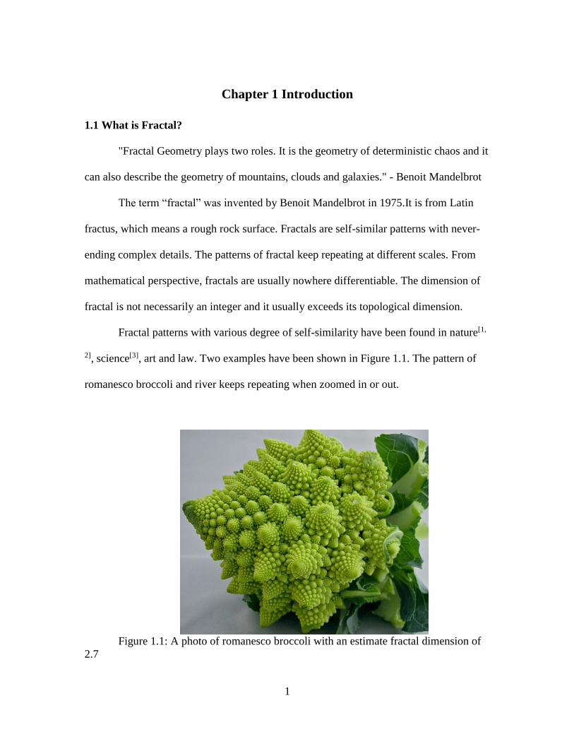
Fractal patterns with various degree of self-similarity have been found in nature[1,

2], science[3], art and law. Two examples have been shown in Figure 1.1. The pattern of

romanesco broccoli and river keeps repeating when zoomed in or out.

Figure 1.1: A photo of romanesco broccoli with an estimate fractal dimension of

2.7

2

The history of fractals began from the 17th century when Gottfried Leibniz, who

was a mathematician and philosopher, meditated recursive self-similarity. Though

Leibniz faultily thought that only the straight line could be self-similar, he raised the term

of “fractional exponents”. However, due to the unfamiliar concepts for different

mathematicians, it was not until the 18th century that researchers involved the function of

fractal graph, published examples of subsets called “Cantor Sets” as fractals, and

introduced a classification of “self-inverse” fractals.

Compared with early researchers who were restricted to manual drawings,

researchers in the late 19th century started to visualize the beauty of fractals because of

the development of computer-based techniques. One of milestones came from the

mathematician Benoît Mandelbrot. In Mandelbrot’s papers, he solidified previous

researchers’ thought and began writing about self-similarity. Mandelbrot made

mathematical development in minting the concept of “fractal” since he constructed

prominent visualizations using computer. His achievement laid a solid foundation for

subsequent research that was exclusively computer-based study on the imagination of

“fractal”.

There are no strict definitions for the concept of fractal amongst authorities.

Mandelbrot himself refer it as “beautiful, damn hard, and increasingly useful. That’s

fractal.” Nowadays, the general agreement is that theoretical fractals are infinitely self-

similar, iterated, and detailed mathematical constructs having fractal dimensions.

Symmetry in our daily language refers to a sense of balance such as reflection,

rotation or translation; while in mathematics, “symmetry” is defined as an object that is

invariant to a transformation. Besides the above three types of transformation, fractal

3

composes of a fourth symmetry, which is the “scaling symmetry”; it is explained by

Mandelbrot “fractals are characterized by so-called “symmetries” which are invariances

under dilations and/or contractions”. It means the roughness and fragmentation of

mathematical or natural fractal shapes will always keep constant as fractal shapes is

zoomed in or out. This characteristic is often referred to as “self-similarity” or “scale

invariance”.

There are plenty of fractal shapes in nature, such as tree branches, vein on a leaf,

our lung capillary structure. They exhibits “roughly” or statistical self-similarity in

different scales, and the scaling is limited in certain range. More structured fractal

patterns are available by recurrence relations and mathematical functions. A good

example of fractal geometry is Sierpinski gasket. The four diagrams shows the process of

creating fractal pattern. The basic step is to divide a black triangle into four sub triangles

and left the middle small triangle out. With infinite division, Sierpinski gasket can be

obtained. The edge of each small triangle is half of the one from ancestor triangle and

self-similarity in preserved by this simple rule of division. The structure remain

unchanged no matter how it is zoomed in or out.

A fractal dimension is an indicator for measuring fractal complexity as a ratio of

the change in detail to the change in scale. It can be non-integer values that may be different

from topological dimensions. With infinite scaling, the geometry of fractal may represent

properties from both integer topological dimensions. For example, a curve with fractal

dimension of 1.1 behaves mostly like a one-dimensional line while one with fractal

dimension of 1.9 will be more likely to behave close to a 2D plane. The calculation of

fractal dimension is shown in Equation 1.1.

4

𝐷 =log(𝑛𝑢𝑚𝑏𝑒𝑟 𝑜𝑓 𝑠𝑒𝑙𝑓−𝑠𝑖𝑚𝑖𝑙𝑎𝑟 𝑝𝑖𝑐𝑒𝑐𝑒𝑠)

log(𝑚𝑎𝑔𝑛𝑖𝑓𝑖𝑐𝑎𝑡𝑖𝑜𝑛 𝑓𝑎𝑐𝑡𝑜𝑟) (1.1)

Sierpinski gasket is a good example for explanation. From first object to second

object in the Figure 1.2, magnification factor should be two and three self-similar pieces

are generated. Take log 3 and log 2 but into Equation 1, the fractal dimension of Sierpinski

gasket is 1.58.

Figure 1.2: Illustration of Sierpinski gasket

During eighteenth and early nineteenth centuries, there was a general census that

every continuous function is with a well-defined tangent at any point or almost all points.

Weierstrass function was the first function that shows it is not the case. Fractal is one of

the functions that nowhere differentiable. Due to infinite scale nature of fractal, fractal is

not differentiable at any point in the domain. With self-similarity, fractal dimension also

stays constant under dilution or contraction.

1.2 Process intensification with fractal distributor

Process intensification is commonly mentioned as one of the most promising

innovation path for chemical process industry. Since its emergence in 1970s, Process

intensification has been attracting extensive research interests from both academic and

industrial societies over the years [4-6]. A simple explanation of Process intensification can

be creating equipment of innovate designs to reduce equipment size and improve efficiency.

Process intensifications (PI) are defined and interpreted in slightly different way by

different industry application and time. In 1983, Ramshaw as one of the pioneers focused

5

exclusively on reduction of equipment size and number of operation units by “PI is the

devising exceedingly compact plant which reduces both the “main plant item” and the

installations cost”;Tsouris and Pocelli in the year of 2003 refer PI as “PI provides radically

innovative principles(“paradigm shift”) in process and equipment design which can

benefit( often with more than a factor of two) process and chain efficiency, capital and

operating expenses, quality, waste, process safety and more.” In 2009, Tom Van Gerv and

Andrzej Stankiewicz,[7] reviewed all the definitions and presented a fundamental vision on

process intensifications with four generic principles regarding spatial, thermodynamic,

functional and temporal domains. One of the generic principles is “give each molecule the

same processing experience.” Processes with all molecules undergo the same history will

deliver uniform products with minimum waste.

Such characteristics are highly demanded by the industrial societies to make

processes more sustainable and environment-friendly[8]. One good example of process

intensification by the principle of “ Giving each molecule the same processing experience”

in chemical industry is the optimization of flow distributors[9]. In many chemical processes,

the uniformity of flow distributions plays the key role in determining the overall

efficiency[10]. Flow distributors usually are installed in chemical equipment, i.e., absorption

column, bubble column and etc., to distribute fluid streams equally. Uniform flow

distributions can enhance the heat / mass transfer rates while reducing material / energy

consumptions[10]; therefore, they can improve the performances of chemical equipment

significantly. In contrast, non-uniformity of flow distributions usually results in

“channeling” phenomenon, i.e., in packed bed[10] or intensifies side reactions inside various

reactors; consequently, the performances of chemical equipment are undermined

6

noticeably. Because of the urgently need, designing novel flow distributors with high

efficiency has become one of the popular issues for process intensification [9, 11-13].

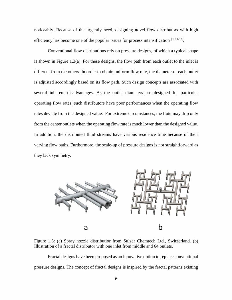
Conventional flow distributions rely on pressure designs, of which a typical shape

is shown in Figure 1.3(a). For these designs, the flow path from each outlet to the inlet is

different from the others. In order to obtain uniform flow rate, the diameter of each outlet

is adjusted accordingly based on its flow path. Such design concepts are associated with

several inherent disadvantages. As the outlet diameters are designed for particular

operating flow rates, such distributors have poor performances when the operating flow

rates deviate from the designed value. For extreme circumstances, the fluid may drip only

from the center outlets when the operating flow rate is much lower than the designed value.

In addition, the distributed fluid streams have various residence time because of their

varying flow paths. Furthermore, the scale-up of pressure designs is not straightforward as

they lack symmetry.

Figure 1.3: (a) Spray nozzle distributior from Sulzer Chemtech Ltd., Switzerland. (b)

Illustration of a fractal distributor with one inlet from middle and 64 outlets.

Fractal designs have been proposed as an innovative option to replace conventional

pressure designs. The concept of fractal designs is inspired by the fractal patterns existing

7

in nature[14], i.e., human’s lung systems, leaf veins and etc. An important feature shared by

these natural patterns is the self-similarity[15]; in other words, these patterns contain pieces

that are duplications of the whole object. By introducing such feature to flow distributors,

fractal distributors utilize symmetric pipe systems to distribute fluid flow. Since such

designs rely on the symmetry rather than the pressure drop, the performances of fractal

distributors remain stable for a wide range of operating flow rates. As their flow paths are

almost identical, the fluid streams exiting from each outlet have narrower residence time

distributions compared to conventional pressure distributors. Besides, such designs are

easy to scale up as well because of their symmetry. In addition to these advantages, fractal

distributors can break down large eddies into smaller ones thus reduce the turbulent

fluctuations. With the generations of branching, the flow inside pipes transits from the

turbulent regime to the laminar one; therefore, the fractal distributors can provide better

control over fluid flow than conventional ones.

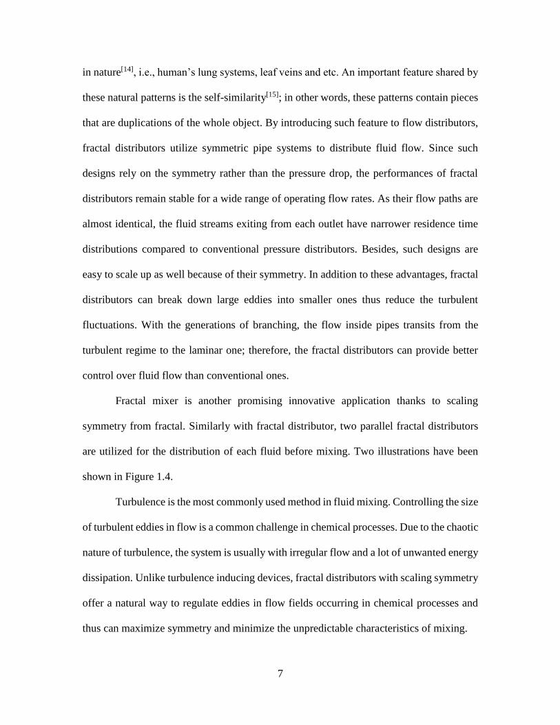
Fractal mixer is another promising innovative application thanks to scaling

symmetry from fractal. Similarly with fractal distributor, two parallel fractal distributors

are utilized for the distribution of each fluid before mixing. Two illustrations have been

shown in Figure 1.4.

Turbulence is the most commonly used method in fluid mixing. Controlling the size

of turbulent eddies in flow is a common challenge in chemical processes. Due to the chaotic

nature of turbulence, the system is usually with irregular flow and a lot of unwanted energy

dissipation. Unlike turbulence inducing devices, fractal distributors with scaling symmetry

offer a natural way to regulate eddies in flow fields occurring in chemical processes and

thus can maximize symmetry and minimize the unpredictable characteristics of mixing.

8

Figure 1.4: Two examples of fractal mixer from Amalgamated Research Inc. website. (a)

A 2 dimensional fractal mixer with two distributors and one collector. Mixing starts at the

junction for two distributors. (b) A 3D fractal mixer with two parallel fluid distributors and

one collector.

1.3 Numerical Modeling of fractal distributor

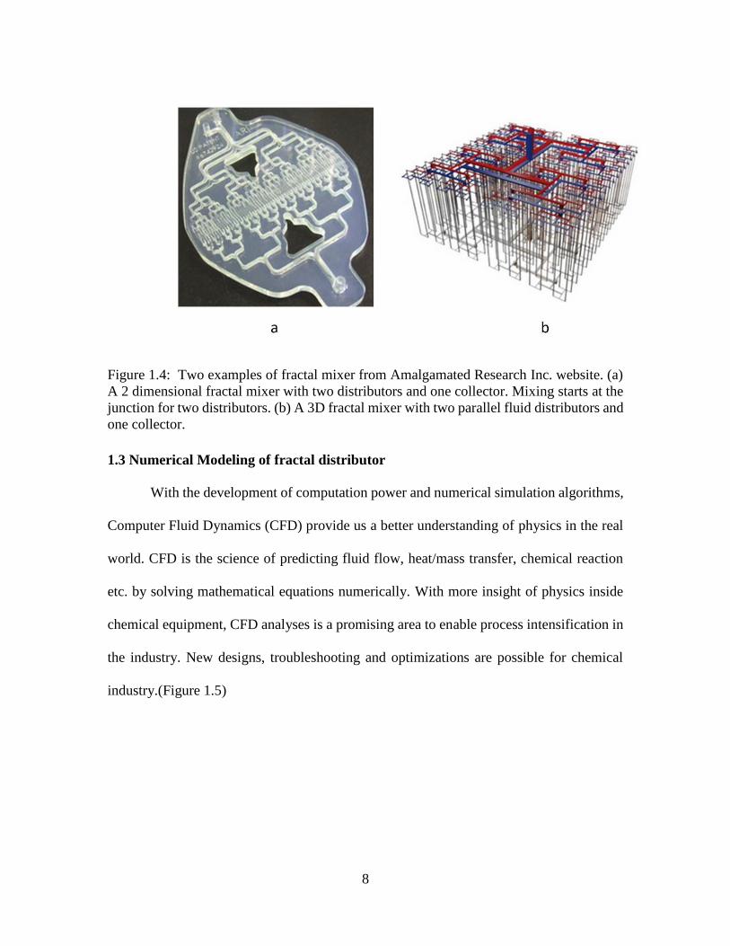
With the development of computation power and numerical simulation algorithms,

Computer Fluid Dynamics (CFD) provide us a better understanding of physics in the real

world. CFD is the science of predicting fluid flow, heat/mass transfer, chemical reaction

etc. by solving mathematical equations numerically. With more insight of physics inside

chemical equipment, CFD analyses is a promising area to enable process intensification in

the industry. New designs, troubleshooting and optimizations are possible for chemical

industry.(Figure 1.5)

9

Figure 1.5: Improvement of Calculations per second per $1000 with time. The

computation power shows an exponential growth as predicted by Moore’s law.

Generally, for simulation of fluid flow in fractal distributor, Navier-Stokes

equation, which is a set of partial differential equation, has been used. For solving

incompressible fluid flow, equation (1.2), (1.3) and (1.4) are needed as listed below.

Equation (1.2) is the continuity equation for conservation of mass. Equation (1.3) and

(1.4) are the Navier-Stokes equations as momentum conservation.

0

v

t

p

(1.2)

𝑡(𝜌 v

) + ∙ (𝜌 v

v

) = −p + ∙ ( ) + 𝜌 Fg

) (1.3)

Where

Ivvv T

3

2 (1.4)

10

At high Reynold’s number where flow is turbulent, there are different turbulent models

that can simply Navier-Stokes equations for higher computation efficiency. In this thesis,

time average methods for simulating turbulent effect have been adopted. Most of the

equations are solved numerically by discretization. Typical numerical methods include

finite difference method (FDM), finite element method (FEM) and finite element (FVM).

Commercial software i.e., ANSYS FLUENT, COMSOL multiphysics, gains more and

more attention with the higher demand from industry as computation capability is

exponentially increasing with time. There are also some open source software available

such as Open Foam.

1.4 Scope of this thesis

This project is seeking to achieve process intensification by designing a novel ion-

exchanger with fractal distributor. With a better understanding of physics, CFD simulations

have been used to optimize the design. The organization of this thesis is as follows: the

second chapter discusses the design and experiments on the novel ion-exchanger device

with fractal distributor. The third chapter is focused on CFD investigations and

optimization for fractal distributor flow distribution on the device.

11

Chapter 2 Experimental Investigation on a Novel Ion-exchanger with

Fractal Distributor

2.1 Introduction

Since its emergence in 1970s, process intensification has been attracting extensive

research interests from both academic and industrial societies over the years [4-6]. By

creating equipment of innovate designs, process intensification on equipment can achieve

higher efficiency and smaller sizes than conventional ones; as a result, it reduces the

material and energy consumptions as well as the waste emissions remarkably. Such

characteristics are highly demanded by the industrial societies to make processes more

sustainable and environment-friendly[8]. One good example of process intensification in

chemical industry is the optimization of flow distributors[9]. In many chemical processes,

the uniformity of flow distributions plays the key role in determining the overall

efficiency[10]. Flow distributors usually are installed in chemical equipment, i.e., absorption

column, bubble column and etc., to distribute fluid streams equally. Uniform flow

distributions can enhance the heat / mass transfer rates while reducing material / energy

consumptions[10]; therefore, they can improve the performances of chemical equipment

significantly. In contrast, non-uniformity of flow distributions usually results in

“channeling” phenomenon, i.e., in packed bed[10] or intensifies side reactions inside various

reactors; consequently, the performances of chemical equipment are undermined

noticeably. Because of the urgently need, designing novel flow distributors with high

efficiency has become one of the popular issues for process intensification[9, 11-13].

Conventional flow distributions rely on pressure designs, of which a typical shape

is shown in Figure 1(A). For these designs, the flow path from each outlet to the inlet is

12

different from the others. In order to obtain uniform flow rate, the diameter of each outlet

is adjusted accordingly based on its flow path. Such design concepts are associated with

several inherent disadvantages. As the outlet diameters are designed for particular

operating flow rates, such distributors have poor performances when the operating flow

rates deviate from the designed value. For extreme circumstances, the fluid may drip only

from the center outlets when the operating flow rate is much lower than the designed value.

In addition, the distributed fluid streams have various residence time because of their

varying flow paths. Furthermore, the scale-up of pressure designs is not straightforward as

they lack symmetry.

Fractal designs have been proposed as an innovative option to replace conventional

pressure designs. The concept of fractal designs is inspired by the fractal patterns existing

in nature[14], i.e., human’s lung systems, leaf veins and etc. An important feature shared by

these natural patterns is the self-similarity[15]; in other words, these patterns contain pieces

that are duplications of the whole object. By introducing such feature to flow distributors,

fractal distributors utilize symmetric pipe systems to distribute fluid flow. Since such

designs rely on the symmetry rather than the pressure drop, the performances of fractal

distributors remain stable for a wide range of operating flow rates. As their flow paths are

almost identical, the fluid streams exiting from each outlet have narrower residence time

distributions compared to conventional pressure distributors. Besides, such designs are

easy to scale up as well because of their symmetry. In addition to these advantages, fractal

distributors can break down large eddies into smaller ones thus reduce the turbulent

fluctuations. With the generations of branching, the flow inside pipes transits from the

13

turbulent regime to the laminar one; therefore, the fractal distributors can provide better

control over fluid flow than conventional ones.

Liquid separation technologies i.e., adsorption, chromatography, ion exchange and

etc. are crucial to bio-refinery industry in process of converting agricultural feedstock to

various products including biofuels, chemicals and etc.. The separation process account for

40-70% of both capital and operating costs in the exist industry. Such process always

includes creating a large uniform surface for possible flow heat/mass transfer or reaction.

Fractal-based technology as a part of process intensification now attracts great attention

and has been commercialized since last decade. Engineering fractal were first applied in

industrial SMB chromatographic column in 1992.And now it has been implemented in

various process, such as juice softening in sugar beet industry, Arkenol process and SMB

(simulated moving bed) Chromatography on biomass conversion stream with system size

reduction factor of 10 , 3 and 2 accordingly[9].

Conventional ion exchangers with ladder distributor usually are designed with

deeper resin beds regardless of process kinetics. In most cases, the extra space is used as a

compensation of poor initial fluid distribution. With resin diameter on the order of 100

micron, a laminar flow will be developed with low radial dispersion. Thus, poor initial

distribution usually leads to a reduction in overall performance. In addition, increasing bed

depth also results in higher-pressure drop and operation cost. Since fractal distributor offers

a much better flow distribution, it allows shallow resin bed approach for ion exchanger

design. It means we can design resin bed depth according to ion-exchange kinetics only

which is very important since it does not only reduce of equipment size, material usage and

pressure drop but also open for more innovation ideas such as high adsorption kinetics

14

resin with smaller diameters. Several implementation of shallow bed approach have been

applied in Sugar industry and reduce the system size significantly[9]. In addition, since

conventional ion-exchanger suffer from poor flow distribution and low contact area with

limited number of outlets. The design may need extra space between distributor and resin

bed as buffer to increase contact area with resin and reduce dead space. However, the extra

liquid space may introduce strong dispersion /backmixing.

With shallow bed approach, the depth of resin bed can be much less than that of

conventional ones. It also comes with a problem; the height of device can be very low

compare with the cross-section area which may rise to space management and manufacture

difficulty since the welding space in the resin bed is too small. A filter press device has

several advantages including highly compacted design, easy to assemble and maintain.

In this paper, a novel filter press based ion-exchange device with fractal distributor

has been designed and manufactured with PMMA. The operating cell consists of seven

plates where internal channels are inter-connected as distributor, resin bed and collector

accordingly. The effect of different outlet density, flow rate has been investigated with dye

injection RTD test. Two different methods of mixing will also be discussed.

2.2 Experimental Setup

2.2.1 Geometry of the Resin Ion-exchange Cell

In this study, we have fabricated an ion-exchange cell using PMMA in

Amalgamated Research Inc. (Figure 2.1). As shown in Figure 2.1, such cell consists of

three components: fractal distributor, resin exchanging section and fractal collector. The

detailed view of the fractal distributor and the resin frame are shown in Figure 2.1. As

illustrated by Figure 2(a, b, c), the fractal distributor is assembled by three plates. The 1st

15

plate contains an H-shape channel that distributes the incoming fluid stream to 4 outlets.

Leaving those outlets, the distributed fluid streams enter the 2nd plate where they are

distributed again to 16 outlets. Similarly on the 3rd plate, the incoming fluid streams are

distributed again to 256 outlets. When they were assembled, these plates were aligned

carefully to ensure that the outlets on the previous plate were connected to the inlets on the

next plate precisely. Silicone gaskets were placed between the plates in order to prevent

leakage.

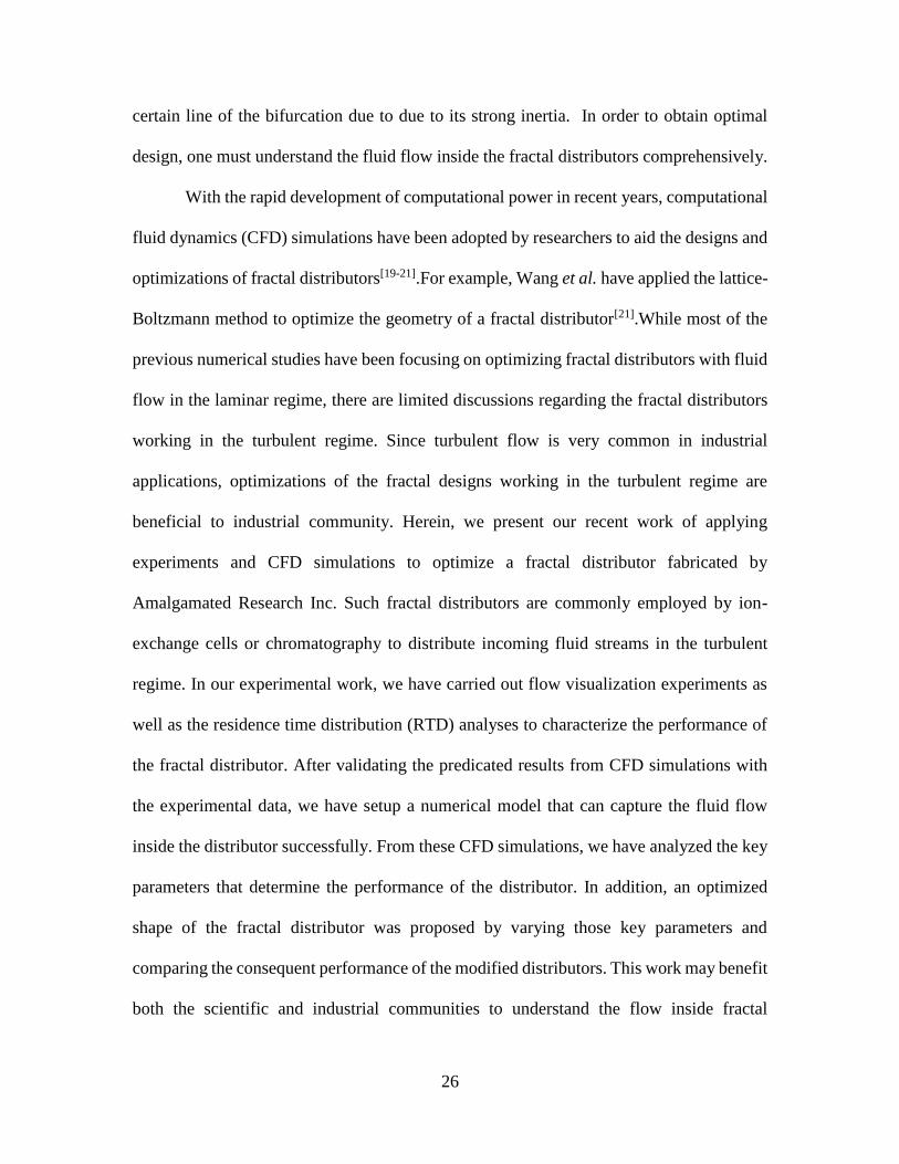
Figure 2.1: Schematic view of the ion-exchange cell (a) the first plate consisting of one

inlet from left and H-shape channel with four outlets (b) the second plate consisting of 16

outlets (c) the third plate consisting 256 outlets with cone shape expansion (d) resin frame

where resin is stuffed in the middle. (e,f,g) collector plates with same geometry as

distributor in a reverse direction. All plates are 12.25-inch square shape and the thickness

of all distributor and collector plates are 1 inch. The thickness of one resin frame is 2

inch.

16

After the distributed fluid streams leave the fractal distributor, they enter the resin

exchanging section. In such section, 310-micron ion-exchange resins are confined inside

the resin frame that is shown in Figure 2.1(d). During the flow visualization experiment,

no resins were added to this section in order to test the efficiency of the fractal distributor

on distributing the fluid streams. If resins were added, this section was sandwiched by two

70-micron meshes so as to prevent the resins from leakage.

After leaving the resin exchanging section, the incoming fluid streams are collected

by the fractal collector. Such collector is identical to the fractal distributor, but the three

plates are assembled in a reverse order. The fluid streams are merged from 256 outlets into

one.

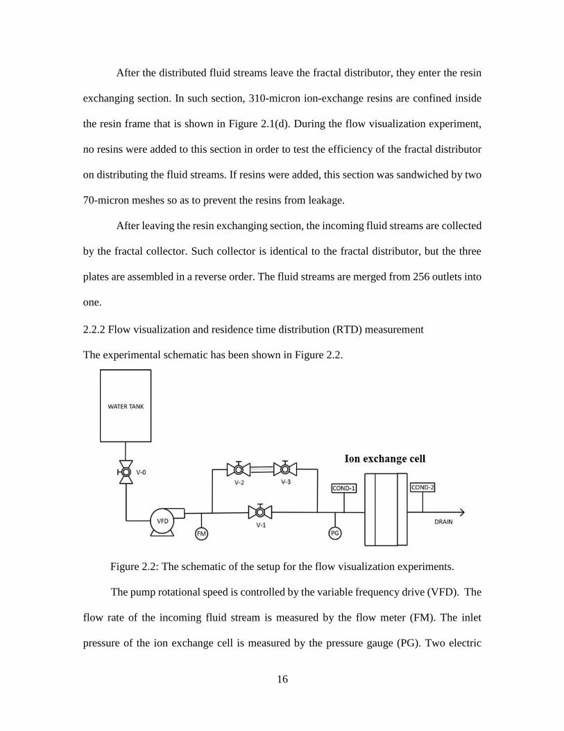
2.2.2 Flow visualization and residence time distribution (RTD) measurement

The experimental schematic has been shown in Figure 2.2.

Figure 2.2: The schematic of the setup for the flow visualization experiments.

The pump rotational speed is controlled by the variable frequency drive (VFD). The

flow rate of the incoming fluid stream is measured by the flow meter (FM). The inlet

pressure of the ion exchange cell is measured by the pressure gauge (PG). Two electric

17

conductivity meters – COND-1 and 2 are placed prior and post the ion exchange cell to

measure the conductivities of the fluid streams entering and leaving the cell. Three valves,

V-1, V-2 and V-3 are placed prior the cell in order to control the injection of dye.

In order to obtain the insightful information about the fluid flow inside the fractal

distributor, the flow visualization experiment and the residence time distribution (RTD)

measurement were carried out with respect to the ion exchange cell. The experimental

setup is illustrated in Figure 2.2. The fluid stream, which was deionized water, was injected

to the ion exchange cell by a centrifugal pump. The rotational speed of the pump was

controlled by a variable frequency drive (VFD) so as to manipulate the injection rate. A

flow meter (FM) was installed on the discharge of the pump to measure the flow rate.

During the experiments, the flow rate of the incoming stream was maintained in the range

of 1 to 4 gallon per minute.

In this study, both the flow visualization experiment and the RTD measurements

were performed simultaneously. The blue dye solution was used to visualize the fluid flow.

Sodium chloride (NaCl) was adopted as the tracer for RTD measurements. The dye

solution and NaCl were premixed to prepare a mixture solution with conductivity of

10mS/cm. Such mixture was introduced to the system via a pipe between valve V-2 and

V-3. During the experiments, the valve V-1 was open initially. At certain time, V-1 was

shut off suddenly; simultaneously, V-2 and V-3 was open to introduce a pulse of dye and

salt solutions to the system. Since the introduction of the NaCl solution altered the

conductivity of the fluid stream, the conductivity values could reflect the tracer

concentration. The conductivity values were measured by two meters: one (COND-1) was

prior to the ion exchange cell; the other (COND-2) was post the cell. The measurements

18

from these two meters were collected and recorder by a computer every 0.03125 s. The

spread of the dye solution was captured by two digital GOPRO cameras: one is placed in

front of the ion exchange cell, and the other is on one side of the cell.The RTD response

and mean residence time tm have been calculated and is shown in Equation 2.1 and 2.2.

𝐸(𝑡) =𝐶(𝑡)

∫ C(t) dt∞

0

(2.1)

𝑡𝑚 = ∫ t E(t) dt∞

0 (2.2)

2.3 Results and discussion

2.3.1 Effect of outlet density on residence time distribution

The basic pattern for fractal distributor is H shape where the flow is evenly

divided. With generations of splitting, incoming flow is distributed uniformly within the

manifold while the momentum of flow is reduced. From mathematical perspective,

fractals have scaling symmetry with infinite divisions; while for engineering fractals, the

generation of division matters considering distribution performance as well as the

manufacture cost and material limitation.

With plate and frame design, fractal distributor are usually consists of three plates

with a total 256 outlets. Since conventional distributors by high pressure design are

usually with less outlets, the first two plates have been assembled to mimic the behavior

of conventional distributor with 16 outlets. Accordingly, the collector at this case is also

changed to 16 inlets with two plates. The test for effect of outlet density can also be

considered as a comparison between fractal distributor and conventional distributor. For

19

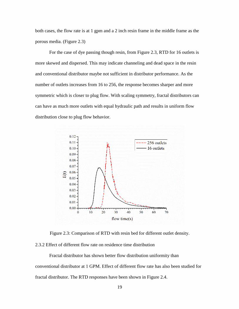
both cases, the flow rate is at 1 gpm and a 2 inch resin frame in the middle frame as the

porous media. (Figure 2.3)

For the case of dye passing though resin, from Figure 2.3, RTD for 16 outlets is

more skewed and dispersed. This may indicate channeling and dead space in the resin

and conventional distributor maybe not sufficient in distributor performance. As the

number of outlets increases from 16 to 256, the response becomes sharper and more

symmetric which is closer to plug flow. With scaling symmetry, fractal distributors can

can have as much more outlets with equal hydraulic path and results in uniform flow

distribution close to plug flow behavior.

Figure 2.3: Comparison of RTD with resin bed for different outlet density.

2.3.2 Effect of different flow rate on residence time distribution

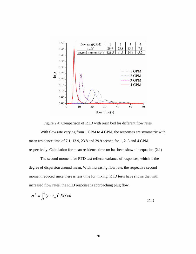
Fractal distributor has shown better flow distribution uniformity than

conventional distributor at 1 GPM. Effect of different flow rate has also been studied for

fractal distributor. The RTD responses have been shown in Figure 2.4.

20

Figure 2.4: Comparison of RTD with resin bed for different flow rates.

With flow rate varying from 1 GPM to 4 GPM, the responses are symmetric with

mean residence time of 7.1, 13.9, 23.8 and 29.9 second for 1, 2, 3 and 4 GPM

respectively. Calculation for mean residence time tm has been shown in equation (2.1)

The second moment for RTD test reflects variance of responses, which is the

degree of dispersion around mean. With increasing flow rate, the respective second

moment reduced since there is less time for mixing. RTD tests have shows that with

increased flow rates, the RTD response is approaching plug flow.

(2.1)

21

2.3.3 Effect of water in pre-distribution

The purpose of distributor is to achieve uniform distribution of fluid on the resin

bed, which is a process to distribute flow from one inlet to distribution area. From the

design perspective, it is ideal to have as many outlets as possible to increase contact area

and approach distribution design geometry. However, it is not practical to have excessive

degree of divisions considering the manufacturing precision and cost. Thus in practice, the

number of outlets is finite and certain degree of mixing have to be provided for a better

distribution.

Conventional ion-exchanger suffer from poor flow distribution and low contact

area with limited number of outlets. The design may need a water layer as buffer to increase

contact area with resin and reduce dead space. However, water layer may introduce strong

dispersion /backmixing. From our experiments, water layer is harmful in providing a

uniform concentration front.

Fractal distributor can provide a uniform distribution with high outlet density and

thus the design does not need water layer. Instead, a cone shape expansion has been

designed to increase contact area.

We compared the dye passing through the middle frame with or without the resin.

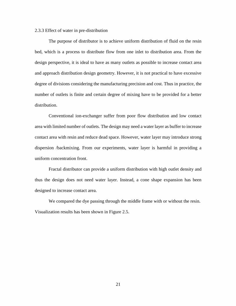
Visualization results has been shown in Figure 2.5.

22

Figure 2.5: Dye profiles for different cases at flow rate of 1 gpm. (a1, a2, a3) the middle

frame consists of one 2 inch water layer and 2 inch resin layer. (b) The middle frame

contains no resin and meshes were installed on both sides of middle frame. (c) 4 inch

resin is filled inside middle frame.

Water layer has been widely used in the industry as a compensation for poor pre-

distribution. The dye mixing process has been shown in Figure 2.5. According to Figure

2.5(a1,a2,a3), it is clear that a uniform dye profile was first created by fractal distributor.

Later, the majority of the dye entered and was stopped by the resin layer. The dye then

showed back mixing within water layer and finally occupied the whole water layer with

homogeneous blue color. Dye need a long time to evacuate from middle frame. Water

layer may introduced strong dispersion /backmixing.

In the design of fractal distributor, a cone shape extension has been adopted for all

the outlets and it can provide local mixing within the cone instead of global mixing in the

water layer. Figure 2.5 (b) shows the dye profile before the dye entered resin bed. Since

there is no way to show dye profile with resin filled inside middle frame, water has been

23

used with meshes for the back pressure at distributor outlets. Similar dye profile can be

expected. The dye occupied all the cones forming a nicely uniform profile. Figure 2.5(c)

showed the actual dye profile with resin filled inside middle frame. It also showed a very

even concentration front. The dye passes through resin quickly.

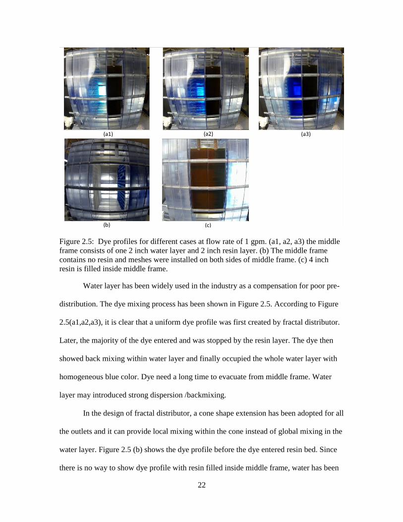
Besides visualization comparison, RTD tests have also been performed. Resin and

water as the media in the 2 inch middle frame have been compared with horizontal flow

rate at 4 GPM (gallon per minute) and with 256 outlets. (Figure 2.6)

Figure 2.6: Comparison of RTD for different media

From Figure 2.6, the RTD response for water and resin shows different patterns.

Water is shown to have more dispersion which is consistent with the observation. Strong

back mixing lead to the wide distribution pattern similar to RTD for CSTR. While for

case of resin, strong isotropic resistance has been formed inside porous media results in a

laminar flow with small dispersion in the transverse direction.

24

From the design perspective, chemical equipment should give each molecule the

same processing experience. Fractal distributor shows plug flow like behavior from both

visualization and RTD response. Water layer used in conventional distributors provides

opportunities for channeling /backmixing and thus is should be avoided in ion-exchanger

design. The introduction of water layer ruined RTD response for fractal distributor.

2.4 Conclusion

In this paper, we have designed and tested a novel filter press based ion-exchanger

with fractal distributor. Fractal distributor solves the problems from conventional

distributor, e.g., poor distribution quality, and small total outlet opening, high pressure drop.

The filter press design also improves the efficiency of space usage for shallow bed

approach.

From visualization and RTD response, fractal distributors can provide plug flow

like concentration front with symmetric RTD response. Reduced outlet density (similar to

conventional distributor) leads reduction of contact area to resin which is prone to have

more resin dead space and thus results in a very skewed RTD response.In addition, the

water buffer layer which is adopted in conventional distributors is shown to be harmful in

providing a uniform concentration front. Instead, the free space may induce large

backmixing as well as channeling.

Fractal distributor greatly enhanced resin utilization efficiency by providing

uniform distribution quality and large total contact area to resin.

25

Chapter 3 Numerical Investigation on a Novel Ion-exchanger with

Fractal Distributor

3.1 Introduction

As discussed in chapter 2, traditional flow distributors are designed based on

pressure drop and thus the RTD responses are very skewed and dispersed due to poor flow

distribution; while thanks to scaling symmetry, fractal distributors exhibit a narrower RTD

response with less back mixing over a wide flow range. Fractal distributor with complex

internal channels is the key for the performance for ion-exchanger. In this chapter, CFD

simulations have been conducted to the existing fractal distributor and parametric study

has been performed for seeking an optimized design.

Although fractal designs are gaining attentions from researchers, there are few

discussions regarding the design or optimization aspects. In 1926, Murray has derived the

best “split ratio”, which was set to 1.27, based on his investigations about the bifurcation

patterns in human vessels. As an important parameter in fractal designs, split ratio is

defined as the cross-sectional area of the pipe in next generation versus that in the previous

one. Such split ratio has been used as a guideline for fractal designs, but it cannot be applied

universally. Most of previous theoretical investigations, i.e., Luo and Tondeur[16-18] focused

on the optimizations of fractal geometries in order to obtain the optimal pressure drops

versus holdup volumes of the flowing channel. These works usually take the assumption

that the fluid stream is equally distributed in each bifurcation; in other words, the fractal

distributors have perfect performance on distributing the fluid streams. Such assumption

contradicts the actual conditions in many circumstances. Especially when the flow is in

turbulent regime, preferential flow occurs that the fluid stream preferentially flows through

26

certain line of the bifurcation due to due to its strong inertia. In order to obtain optimal

design, one must understand the fluid flow inside the fractal distributors comprehensively.

With the rapid development of computational power in recent years, computational

fluid dynamics (CFD) simulations have been adopted by researchers to aid the designs and

optimizations of fractal distributors[19-21].For example, Wang et al. have applied the lattice-

Boltzmann method to optimize the geometry of a fractal distributor[21].While most of the

previous numerical studies have been focusing on optimizing fractal distributors with fluid

flow in the laminar regime, there are limited discussions regarding the fractal distributors

working in the turbulent regime. Since turbulent flow is very common in industrial

applications, optimizations of the fractal designs working in the turbulent regime are

beneficial to industrial community. Herein, we present our recent work of applying

experiments and CFD simulations to optimize a fractal distributor fabricated by

Amalgamated Research Inc. Such fractal distributors are commonly employed by ion-

exchange cells or chromatography to distribute incoming fluid streams in the turbulent

regime. In our experimental work, we have carried out flow visualization experiments as

well as the residence time distribution (RTD) analyses to characterize the performance of

the fractal distributor. After validating the predicated results from CFD simulations with

the experimental data, we have setup a numerical model that can capture the fluid flow

inside the distributor successfully. From these CFD simulations, we have analyzed the key

parameters that determine the performance of the distributor. In addition, an optimized

shape of the fractal distributor was proposed by varying those key parameters and

comparing the consequent performance of the modified distributors. This work may benefit

both the scientific and industrial communities to understand the flow inside fractal

27

distributors. The numerical model used in this work can be applied to optimize the fractal

distributors in other applications as well.

3.2 Numerical simulations setup

3.2.1 Plates Design of Ion-exchanger with Fractal Distributor

In this study, we have fabricated an ion-exchange cell using PMMA in

Amalgamated Research Inc.. As shown in Figure 3.1, such cell consists of three

components: fractal distributor, resin exchanging section and fractal collector. The detailed

view of the fractal distributor and the resin frame are shown in Figure 3.1. As illustrated

by Figure 2(a, b, c), the fractal distributor is assembled by three plates. The 1st plate

contains an H-shape channel that distributes the incoming fluid stream to 4 outlets. Leaving

those outlets, the distributed fluid streams enter the 2nd plate where they are distributed

again to 16 outlets. Similarly on the 3rd plate, the incoming fluid streams are distributed

again to 256 outlets. When they were assembled, these plates were aligned carefully to

ensure that the outlets on the previous plate were connected to the inlets on the next plate

precisely. Silicone gaskets were placed between the plates in order to prevent leakage.

After the distributed fluid streams leave the fractal distributor, they enter the resin

exchanging section. In such section, 310-micron ion-exchange resins are confined inside

the resin frame that is shown in Figure 3.1(d). During the flow visualization experiment,

no resins were added to this section in order to test the efficiency of the fractal distributor

on distributing the fluid streams. If resins were added, this section was sandwiched by two

70-micron meshes so as to prevent the resins from leakage.

28

Figure 3.1: Schematic view of the ion-exchange cell (a) the first plate consisting of one

inlet from left and H-shape channel with four outlets (b) the second plate consisting of 16

outlets (c) the third plate consisting 256 outlets with cone shape expansion (d) resin frame

where resin is stuffed in the middle. (e, f, g) collector plates with same geometry as

distributor in a reverse direction. All plates are 12.25-inch square shape and the thickness

of all distributor and collector plates are 1 inch. The thickness of one resin frame is 2

inch.

After leaving the resin exchanging section, the incoming fluid streams are collected

by the fractal collector. Such collector is identical to the fractal distributor, but the three

plates are assembled in a reverse order. The fluid streams are merged from 256 outlets into

one.

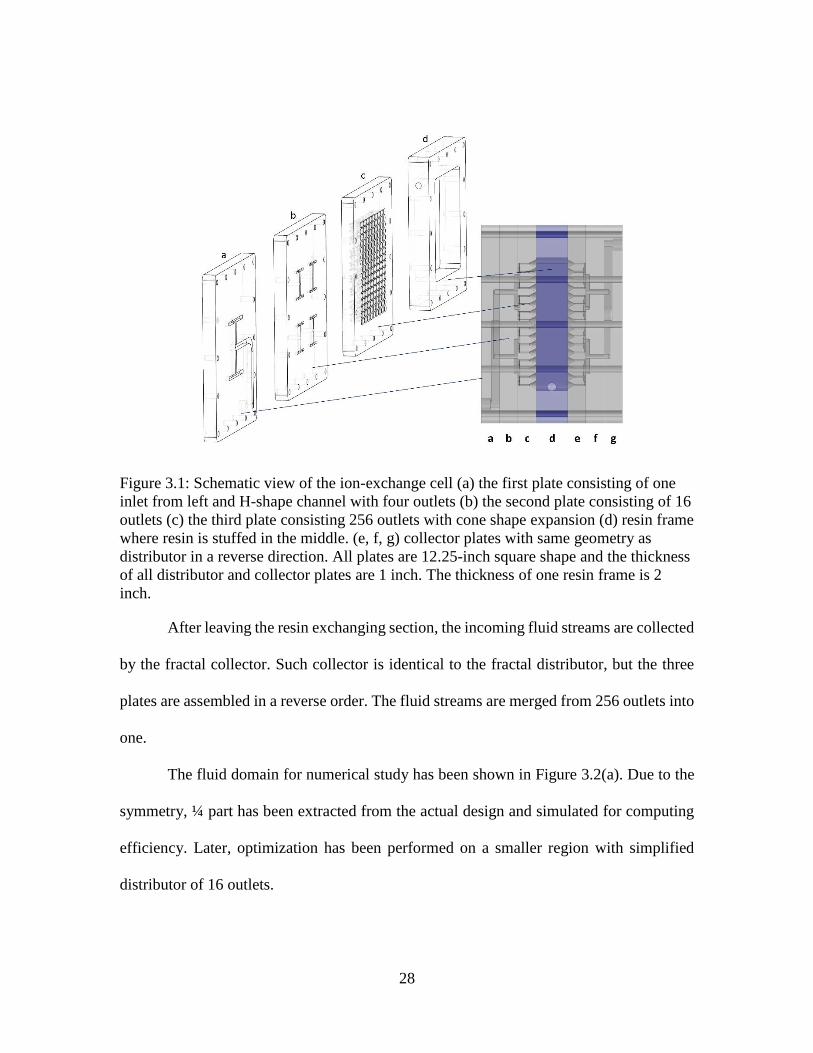
The fluid domain for numerical study has been shown in Figure 3.2(a). Due to the

symmetry, ¼ part has been extracted from the actual design and simulated for computing

efficiency. Later, optimization has been performed on a smaller region with simplified

distributor of 16 outlets.

29

Figure 3.2: The fluid domains for numerical study. (a)The domain consists of three parts;

a distributor (blue top), porous media (green) and collector (blue bottom). A symmetry

boundary condition has been applied to yellow region. One inlet and one outlet are

located at the top and bottom corner. (b) Top and side view of the local flow domain with

16 outlets from (a). Dimensions are shown with mm as unit. Optimization has been

performed based on (b).

3.2.2 Numerical Methods

CFD simulations on fluid flow inside the device are mainly based on k-epsilon

turbulent model. The validation of residence time distribution coupled species transport

equation with turbulent model equations. For the porous media, an additional momentum

source term into Navier-Stokes equation is used for fluid flow and Ergun equation is used

for pressure drop across the porous media.

3.2.2.1 The Continuity Equation for Mass Conservation

The equation describes mass conservation across control volume for unsteady

flow as is shown in equation (3.1).

30

0

tz

v

y

v

x

v zyx (3.1)

Where xv , yv , and zv are the fluid velocities in the x, y, and z directions,

respectively. This equation can also be written in vector notation as:

0

v

t

p

where is the divergence. (3.2)

3.2.2.2 The Continuity Equation for Momentum Conservation

𝑡(𝜌 v

) + ∙ (𝜌 v

v

) = −p + ∙ ( ) + 𝜌 Fg

(3.3)

Ivvv T

3

2 (3.4)

3.2.2.3 Realizable K-Epsilon model for turbulent flow

With the given inlet flow rate, the incoming flow is in turbulent region. For CFD

simulation, Realizable K-Epsilon model have been adopted. The k-epsilon model is most

commonly used in CFD to simulate the mean flow characteristics for turbulent flow. Since

it would be very computationally costly to model turbulent eddies in small scale under high

frequency fluctuations, time average models (RANS) for simulation of turbulent flow has

been derived. In these models, terms for average turbulent flow field have been introduced

and thus smaller scale turbulent behaviors will not appear in main Navier Stokes equations.

For k-epsilon turbulent model, turbulent kinetic energy k and turbulent dissipation rate

epsilon must be determined. And thus we need to solve two additional closure models

besides Navier Stokes time averaged equations. With the reduction of mathematics, RANS

turulent models gain popularity among industrial projects since it can significantly reduce

31

the processing time and thus improve computing efficiency. Velocity at any time can be

decomposed as (3.5).

'vvv (3.5)

where v is the mean velocity, and 'v accounts for the turbulent fluctuation .

The Reynolds-averaged Navier-Stokes equations can be derived with (3.6) and

(3.7).

0

i

i

uxt

(3.6)

ji

jl

l

ij

i

j

j

i

ji

ji

j

i uuxx

u

x

u

x

u

xx

puu

xu

t''

3

2

(3.7)

The two-equation RANS turbulence models uses Boussinesq hypothesis by

assuming momentum transfer caused by turbulent eddies can be modeled with an eddy

viscosity t . The Boussinesq assumption states that the Reynolds stress tensor, ij , is

proportional to the trace-less mean strain rate tensor, ijS.

ij

k

k

t

i

j

j

i

tjix

uk

x

u

x

uuu

3

2'' . (3.8)

Since the Boussinesq hypothesis is based on assuming Reynolds stress tensor is

proportional to the strain rate tensor which may be invalid for flow with strong

accelerations or swirls.

The standard k-epsilon model is a simple yet robust two-equation turbulence

model that has been utilized widely in industry for practical flow analyses over the years.

32

kMbk

jk

t

j

i

i

SYGGx

k

xku

xk

t

(3.9)

S

kCGCG

kC

xxu

xtbk

j

t

j

i

i

2

231

(3.10)

Where turbulent viscosity, production of k and mean strain rate tensor is calculated

as

2kCt . (3.11)

i

j

jikx

uuuG

'' (3.12)

ijij SSS 2 (3.13)

In this thesis, k- realizable turbulence model has been adopted with advantages

such as improved performance in flows with recirculation, strong pressure gradients, and

flow separation.

Different formulation for turbulent viscosity has been applied in realizable

turbulence model with comes from mean square vorticity fluctuation.

kMbk

jk

t

j

j

j

SYGGx

k

xku

xk

t

(3.14)

SGC

kC

vkCSC

xxu

xtb

j

t

j

j

j

31

2

21

(3.15)

33

In this case C is not a constant. It is instead calculated from

*

0

1

kUAA

C

S

(3.16)

Where

ijijijij SSU ~~*

(3.17)

ANSYS FLUENT has been used in CFD simulations. For simulation of flow pass

through resin bed, porosity is set as 0.47 with 4.51E9 as viscous resistance and 5.96E4 as

inertial resistance. For turbulent flow, scalable wall function has been used. Inlet velocity

is set as 0.415, 0.83, 1.245 and 1.660 m/s for 1, 2, 3 and 4 GPM flow rate. No slip wall

boundary condition has been applied. Mesh is generated with cut cell method in ANSYS

MESHING with 2.8 million elements. SIMPLE(Semi-Implicit Method for Pressure-

Linked Equations) scheme was used for pressure-velocity coupling of the momentum

equations and continuity equations. For spatial discretization, Least Squares Cell Based

method has been adopted for gradient; Standard method has been used for Pressure

interpolation; First Order Upwind has been used for momentum, turbulent kinetic energy

and turbulent dissipation rate. Under-Relaxation Factors for pressure and momentum are

0.3 and 0.5 respectively. With these configurations, a steady state solution has been

calculated and analyzed. Post-processing has been performed by ANSYS CFD-POST and

TECPLOT.

3.3 CFD Modeling Validation

The red curve is RTD response from the experiments at 4 gpm, and the blue curve

is the response from the experiments. The result shows a good match between experiments

34

and simulation. The mean residence time for experiment and CFD are 7.06s and 7.10s

respectively. CFD simulation is proves to be efficient in predicting the experiment results

(Figure 3.2).

Figure 3.2: RTD response for experiment and CFD simulation at flow rate of 4gpm.

Mesh independence study has been performed. Flow rates for 8 outlets in one line

have been listed in Figure 3.3.With increasing mesh density, from 1.54 million to 8 million

mesh elements, the flow rates stop changing at 2.8 million elements which is consider

appropriate for CFD simulations in the chapter. The mesh density of 2.8 million elements

has been applied to the rest of CFD simulations. Ideally the flow rates should be the same

for all the outlets for distributor. While, from Figure 3.3, there is not too much change from

outlet 1 to outlet 7 and there is a sudden jump for flow at outlet 8. Further inspection will

be conducted on this issue.

-1.0E-01

0.0E+00

1.0E-01

2.0E-01

3.0E-01

4.0E-01

5.0E-01

6.0E-01

1 6 11 16

E(t)

Time(s)

CFD Validation e(t) from CFDsimulation

e(t) from experiment

35

Figure 3.3: (a) flow rate at different outlets with different mesh density. (b) Illustration of

outlet positions. Outlets with red color are listed as outlet 1 to 8 from top to bottom.

3.4 Results and Discussion

Uniformity of flow distribution is the major concern for flow distributor and it is

the key factor for the overall device performance. To evaluate flow uniformity, different

method from experiments and simulations have been involved. In the experiments, since

there is no way to obtain the information of flow rates at outlets from the experiments,

indirect methods such as RTD response and snapshot of dye profile were used to

characterize the performance of flow distribution. A narrow RTD response with

observation of a plug flow like concentration front indicates a good flow distribution from

distributor.

CFD simulations show its advantages for design and troubleshooting. The flow

rates for all the outlets can collect and based on the information, coefficient of variation

has been calculated. It is defined as the ratio of the standard deviation to the mean.

36

Coefficient of variation (COV) is a better way to quantify the performance of fractal

distributor than RTD response.

In the validation part, we have successfully proved that the models used in this

chapter can predict flow behavior accurately. While for optimization purpose, a parametric

study has been performed based on a reduced model from the actual geometry. Assume

uniform flow bifurcated at first two T-junction, and the backpressure is high on the resin

side that provides a homogeneous outlet condition for the distributor. A reduced model has

been proposed. The dimensions are shown in Figure 3.4. All the numerical setting from

preview model is kept constant in this new model. The reduced model is with one inlet and

16 outlets. Inlet velocity is set as 0.288, 0.576, 0.864 and 1.15 m/s according to flow rate

to 1, 2, 3 and 4 gpm.

Figure 3.4: Geometry of reduced model. Dimensions are with unit of mm.

With the dimensions from existing design, parametric study has been performed.

From Figure 3.4(a), channel width may change at bifurcation. For example, the channel

width is 5.232 mm for the main inlet, and it is 4.064, 3.153, 2.543, 2.384, and 2.384

respectively for further bifurcations. In general, the channel width becomes smaller with

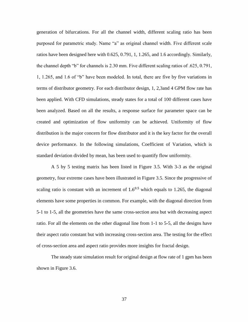
37

generation of bifurcations. For all the channel width, different scaling ratio has been

purposed for parametric study. Name “a” as original channel width. Five different scale

ratios have been designed here with 0.625, 0.791, 1, 1.265, and 1.6 accordingly. Similarly,

the channel depth “b” for channels is 2.30 mm. Five different scaling ratios of .625, 0.791,

1, 1.265, and 1.6 of “b” have been modeled. In total, there are five by five variations in

terms of distributor geometry. For each distributor design, 1, 2,3and 4 GPM flow rate has

been applied. With CFD simulations, steady states for a total of 100 different cases have

been analyzed. Based on all the results, a response surface for parameter space can be

created and optimization of flow uniformity can be achieved. Uniformity of flow

distribution is the major concern for flow distributor and it is the key factor for the overall

device performance. In the following simulations, Coefficient of Variation, which is

standard deviation divided by mean, has been used to quantify flow uniformity.

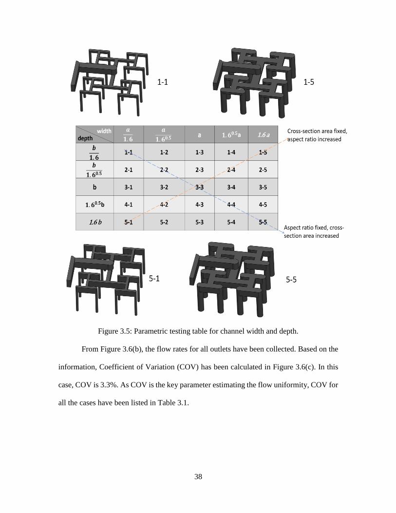
A 5 by 5 testing matrix has been listed in Figure 3.5. With 3-3 as the original

geometry, four extreme cases have been illustrated in Figure 3.5. Since the progressive of

scaling ratio is constant with an increment of 1.60.5 which equals to 1.265, the diagonal

elements have some properties in common. For example, with the diagonal direction from

5-1 to 1-5, all the geometries have the same cross-section area but with decreasing aspect

ratio. For all the elements on the other diagonal line from 1-1 to 5-5, all the designs have

their aspect ratio constant but with increasing cross-section area. The testing for the effect

of cross-section area and aspect ratio provides more insights for fractal design.

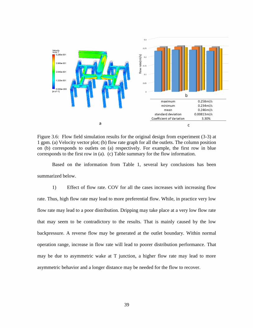
The steady state simulation result for original design at flow rate of 1 gpm has been

shown in Figure 3.6.

38

Figure 3.5: Parametric testing table for channel width and depth.

From Figure 3.6(b), the flow rates for all outlets have been collected. Based on the

information, Coefficient of Variation (COV) has been calculated in Figure 3.6(c). In this

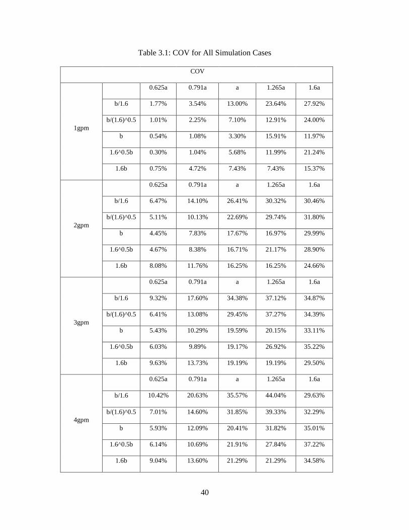
case, COV is 3.3%. As COV is the key parameter estimating the flow uniformity, COV for

all the cases have been listed in Table 3.1.

39

Figure 3.6: Flow field simulation results for the original design from experiment (3-3) at

1 gpm. (a) Velocity vector plot; (b) flow rate graph for all the outlets. The column position

on (b) corresponds to outlets on (a) respectively. For example, the first row in blue

corresponds to the first row in (a). (c) Table summary for the flow information.

Based on the information from Table 1, several key conclusions has been

summarized below.

1) Effect of flow rate. COV for all the cases increases with increasing flow

rate. Thus, high flow rate may lead to more preferential flow. While, in practice very low

flow rate may lead to a poor distribution. Dripping may take place at a very low flow rate

that may seem to be contradictory to the results. That is mainly caused by the low

backpressure. A reverse flow may be generated at the outlet boundary. Within normal

operation range, increase in flow rate will lead to poorer distribution performance. That

may be due to asymmetric wake at T junction, a higher flow rate may lead to more

asymmetric behavior and a longer distance may be needed for the flow to recover.

40

Table 3.1: COV for All Simulation Cases

COV

1gpm

0.625a 0.791a a 1.265a 1.6a

b/1.6 1.77% 3.54% 13.00% 23.64% 27.92%

b/(1.6)^0.5 1.01% 2.25% 7.10% 12.91% 24.00%

b 0.54% 1.08% 3.30% 15.91% 11.97%

1.6^0.5b 0.30% 1.04% 5.68% 11.99% 21.24%

1.6b 0.75% 4.72% 7.43% 7.43% 15.37%

2gpm

0.625a 0.791a a 1.265a 1.6a

b/1.6 6.47% 14.10% 26.41% 30.32% 30.46%

b/(1.6)^0.5 5.11% 10.13% 22.69% 29.74% 31.80%

b 4.45% 7.83% 17.67% 16.97% 29.99%

1.6^0.5b 4.67% 8.38% 16.71% 21.17% 28.90%

1.6b 8.08% 11.76% 16.25% 16.25% 24.66%

3gpm

0.625a 0.791a a 1.265a 1.6a

b/1.6 9.32% 17.60% 34.38% 37.12% 34.87%

b/(1.6)^0.5 6.41% 13.08% 29.45% 37.27% 34.39%

b 5.43% 10.29% 19.59% 20.15% 33.11%

1.6^0.5b 6.03% 9.89% 19.17% 26.92% 35.22%

1.6b 9.63% 13.73% 19.19% 19.19% 29.50%

4gpm

0.625a 0.791a a 1.265a 1.6a

b/1.6 10.42% 20.63% 35.57% 44.04% 29.63%

b/(1.6)^0.5 7.01% 14.60% 31.85% 39.33% 32.29%

b 5.93% 12.09% 20.41% 31.82% 35.01%

1.6^0.5b 6.14% 10.69% 21.91% 27.84% 37.22%

1.6b 9.04% 13.60% 21.29% 21.29% 34.58%

41

2) With channel width fixed, the optimum channel depth is different based on

width. For 0.625a, the minimum COV appears at depth of “b” for most of the cases. While,

at 0.791a, at flow rate of 1 and 2 gpm, the optimum depth is “b” and for flow rate of 3 and

4 gpm, the best depth is 1.265b. It seems that there is a shift effect that the optimum depth

increase with the increase of scaling in “a” and flow rate. For width scale higher than

0.791”a”, there is a monotonous decrease of COV with increase of depth. That also verify

the finding mentioned above.

3) With channel depth fixed, in most cases increasing width will undermine

the distribution performance. A wider turn at every bifurcation is prone to have preferential

flow considering channeling may happen due to inertia.

4) For fixing aspect ratio, decrease in cross-section area will increase flow

uniformity. That may indicate that a bigger channel is not helpful to improve the design.

On the other hand, pressure drop should also be considered.

5) For fixing cross-section area, a larger depth to width ratio shows better COV.

That may due to the fact that, high aspect ratio channel are narrower and deeper in depth.

It may help the flow to return to neutral state after T junction.

6) For the overall performance, channel depth of “b” and channel width of

0.625 “a” is recommended with the lowest COV.

7) Pressure drop discussion for fractal distributor is not as important as COV,

because it is usually very extremely low which not the limiting factor in the design is. For

highest flow rate (4gpm), and smallest cross-section area (1-1 configuration), the pressure

drop across the device is 5.35KPa.

42

3.5 Design Defects Detection by CFD

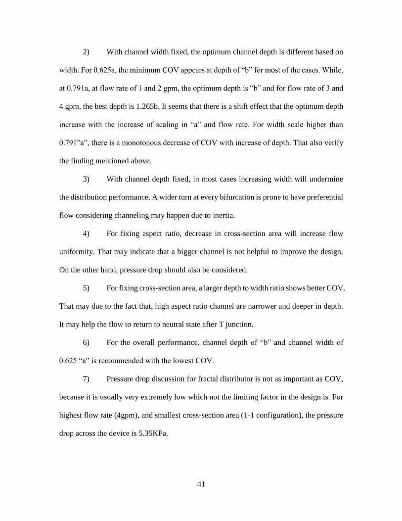
With CFD simulations, some defects from original ion-exchanger design have

been detected. One problem with resin area will be discussed in this section. The model is

based on the device from the experiment and with the help of CFD, the distribution of flow

at outlets has been shown in Figure 3.7, 3.8 and Table 3.2. The distribution coefficient of

variation is 7.1%. The flow rates of outlets on the edge are higher than the ones in the

middle. That is due to the geometry distribution inconsistency. The outlets on the edge

have more resin space for flow to be distributed resulting in less resistance compare with

the ones in the middle. And as a result, the flow rate is higher.

Figure 3.7: Velocity magnitude plot in the resin for 0.1 inch away from the outlets. The

velocity near the region of outlets on the edge shows highest magnitude.

Since flow maldistribution is caused by both geometry of the resin and the

configuration of the distributor that is the main interest. A modified model has been

purposed with cut resin area according to the actual distribution area. So COV for cut

model is caused only by the configuration of the fractal distributor.

43

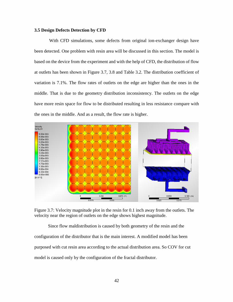
Table 3.2. Statistics for Table 6

max 1.19300E+00 ml/s

min 9.12600E-01 ml/s

max/min 1.307254

mean flow 9.71040E-01 ml/s

std 6.85582E-02 ml/s

COV 7.1%

Figure 3.8: 3D plot for flow rate at each outlet.

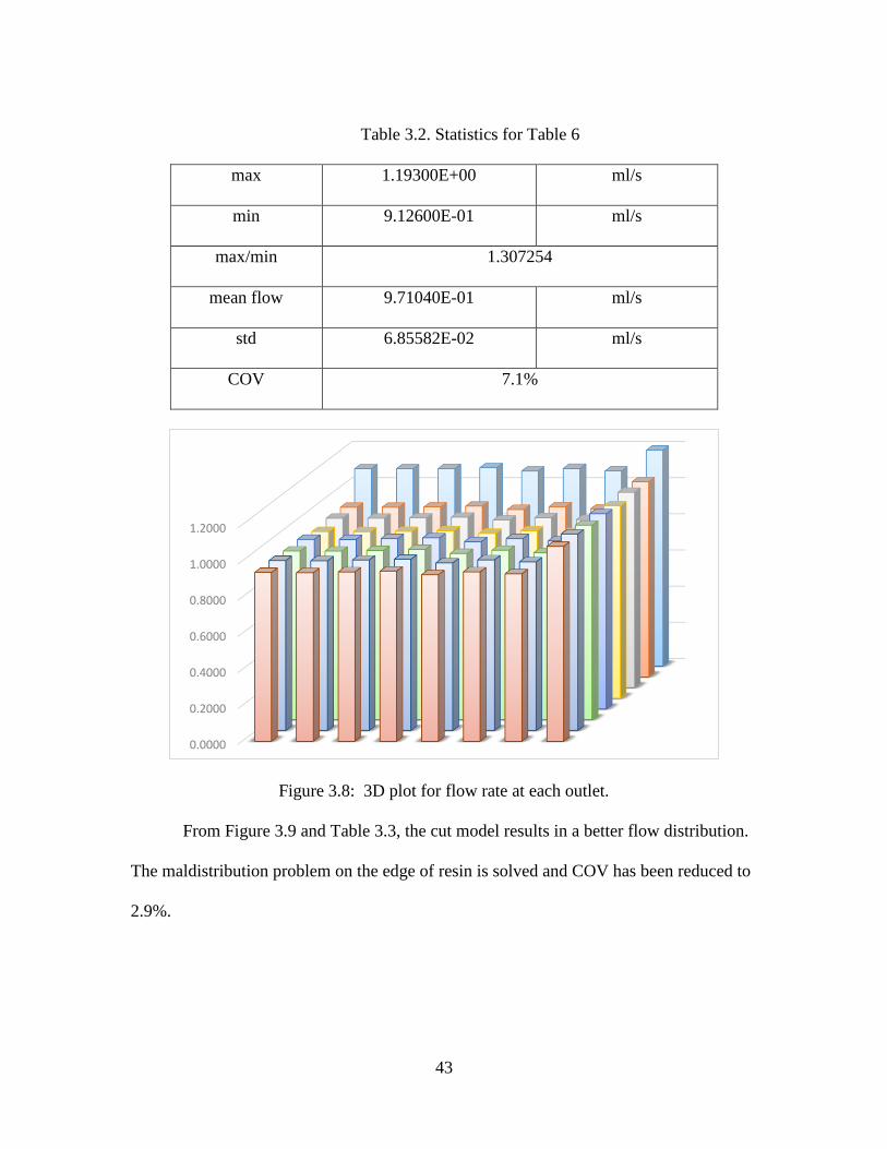
From Figure 3.9 and Table 3.3, the cut model results in a better flow distribution.

The maldistribution problem on the edge of resin is solved and COV has been reduced to

2.9%.

0.0000

0.2000

0.4000

0.6000

0.8000

1.0000

1.2000

44

Figure 3.9: Velocity magnitude plot in the resin for 0.1 inch away from the outlets.

Table 3.3: Statistics for Table 8

max 1.05300E+00 ml/s

min 9.16400E-01 ml/s

max/min 1.149061545

mean flow 9.97556E-01 ml/s

std 2.90838E-02 ml/s

COV 2.9%

3.6 Conclusion

In this chapter, CFD simulations have been conducted with parametric study on the

novel ion-exchanger with fractal distributor. Coefficient of variation is the key parameter

for estimating the performance of fractal distributor.

Parametric study has been performed based on five different channel width, five

different channel depth at four different flow rate. Increase in flow rate will lead to increase

of COV. Channel width appears to be critical in fractal distributor design. Decrease in

channel width will result in the reduction of COV for all the cases. In addition, with channel

width fixed, the optimum channel depth is different based on width and flow rate. COV is

45

not as sensitive on channel depth as it is on channel width. For the overall performance,

channel depth of “b” and channel width of 0.625 “a” are recommended with the lowest

COV.

With the rapid growth of computation power, CFD simulations can help us

understand the physics inside chemical equipment as well as provide optimization to the

design.

46

References

[1] C.O. Tan, M.A. Cohen, D.L. Eckberg, J.A. Taylor, Fractal properties of human heart

period variability: physiological and methodological implications, The Journal of

Physiology 587 (2009) 3929-3941.

[2] J.Z. Liu, L.D. Zhang, G.H. Yue, Fractal Dimension in Human Cerebellum Measured

by Magnetic Resonance Imaging, Biophysical Journal 85 4041-4046.

[3] P. Vannucchi, L. Leoni, Structural characterization of the Costa Rica décollement:

Evidence for seismically-induced fluid pulsing, Earth and Planetary Science Letters 262

(2007) 413-428.

[4] V. Hessel, Novel Process Windows – Gate to Maximizing Process Intensification via

Flow Chemistry, Chemical Engineering & Technology 32 (2009) 1655-1681.

[5] A.I. Stankiewicz, J.A. Moulijn, Process intensification: Transforming chemical

engineering, Chemical Engineering Progress 96 (2000) 22-34.

[6] J.-C. Charpentier, In the frame of globalization and sustainability, process

intensification, a path to the future of chemical and process engineering (molecules into

money), Chemical Engineering Journal 134 (2007) 84-92.

[7] T. Van Gerven, A. Stankiewicz, Structure, Energy, Synergy, Time—The

Fundamentals of Process Intensification, Industrial & Engineering Chemistry Research

48 (2009) 2465-2474.

[8] H. Liu, X. Liang, L. Yang, J. Chen, Challenges and innovations in green process

intensification, Sci. China Chem. 53 (2010) 1470-1475.

[9] V. Kochergin, M. Kearney, Existing biorefinery operations that benefit from fractal-

based process intensification, Appl Biochem Biotechnol 130 (2006) 349-360.

[10] A. Jiao, S. Baek, Effects of Distributor Configuration on Flow Maldistribution in

Plate-Fin Heat Exchangers, Heat Transfer Engineering 26 (2005) 019-025.

[11] M. Kearney, Control of Fluid Dynamics with Engineered Fractals-Adsorption

Process Applications, Chemical Engineering Communications 173 (1999) 43-52.

[12] M.M. Kearney, Engineered fractals enhance process applications, Chemical

Engineering Progress 96 (2000) 61-68.

47

[13] M.M. Kearney, M.W. Mumm, K.R. Petersen, T. Vervloet, Fluid transfer system with

uniform fluid distributor, Google Patents, 1994.

[14] A. Bejan, S. Lorente, Constructal law of design and evolution: Physics, biology,

technology, and society, Journal of Applied Physics 113 (2013) 151301.

[15] B. Mandelbrot, The fractal geometry of nature, W.H. Freeman1982.

[16] D. Tondeur, Y. Fan, L. Luo, Constructal optimization of arborescent structures with

flow singularities, Chemical Engineering Science 64 (2009) 3968-3982.

[17] D. Tondeur, L. Luo, Design and scaling laws of ramified fluid distributors by the

constructal approach, Chemical Engineering Science 59 (2004) 1799-1813.

[18] L. Luo, D. Tondeur, Optimal distribution of viscous dissipation in a multi-scale

branched fluid distributor, International Journal of Thermal Sciences 44 (2005) 1131-

1141.

[19] L. Wang, Y. Fan, L. Luo, Lattice Boltzmann method for shape optimization of fluid

distributor, Computers & Fluids 94 (2014) 49-57.

[20] Z. Fan, X. Zhou, L. Luo, Numerical Investigation of Constructal Distributors with

Different Configurations, (2009).

[21] L. Wang, Y. Fan, L. Luo, Lattice Boltzmann method for shape optimization of fluid

distributor, Computers & Fluids 94 (2014) 49-57.

48

Vita

Gongqiang He was born in Xiongyue, Liaoning, China. In 2006, he entered Dalian

University of Technology and received his bachelor’s degree in the year of 2010.

Thereafter, he became a graduate student in Louisiana State University. He will receive

his master’s degree in May 2015.