Application ofX-Ray PulsarNavigation: A

Characterization ofthe Earth OrbitTrade Space

Wayne H. Yu, Navigation and Mission Design Branch,NASA Goddard Space Flight Center

BiographyMr. Wayne Yu is a flight dynamics engineer at theNASA Goddard Spaceflight Center in the navigationand mission design branch. He is involved in variousflight projects in both trajectory design and navi-gation. Projects include libration point trajectorydesign for the James Webb Space Telescope and theARTEMIS mission, formation flight design with theMagnetospheric MultiScale Mission, and stochasticestimation and navigation design with the SEXTANTmission. He received his B.S. in 2010 and then his M.S.in 2015 in Aerospace Engineering at the University ofMaryland, College Park.

AbstractX-ray pulsar navigation (XNAV) is a celestial naviga-tion system that uses the consistent timing nature ofX-ray photons from milli-second pulsars (MSP) to per-form space navigation. The challenge of XNAV comesfrom the faint signal, availability, and distant natureof pulsars. This paper is a study of extended Kalmanfilter (EKF) tracking performance within a wide tradespace of bounded Earth orbits using only XNAV mea-surements. The study uses a simulation of existing X-ray detector space hardware. An example of an X-raydetector for XNAV is the NASA Station Explorer forX-ray Timing and Navigation (SEXTANT) mission, atechnology demonstration of XNAV set to perform onthe International Space Station (ISS) in 2017.This study in particular defines the Earth orbits as Ke-plernian elements and varies each element individuallyto observe XNAV performance. It shows that the closedEarth orbit for XNAV performance relies on the orbitsemi-major axis and eccentricity as well as orbit inclina-tion. These parameters drive pulsar measurement avail-ability and quality by influencing the natural spacecraftorbit dynamics. The orbit angles of argument of perigeeand right ascension of the ascending node help definethe orbit and its initial XNAV measurements. Sensi-tivity to initial orbit determination error growth dueto the scarcity of XNAV measurements within an or-bital period require appropriate timing of initial XNAVmeasurements.

List of Abbreviations

AOP Argument of Periapsis

CRLB Cramer-Rao Lower Bound

ECI Earth Centered Inertial

ECC Eccentricity

EKF Extended Kalman Filter

GEO Geosynchronous Earth Orbit

GMAT General Mission Analysis Tool

INC Inclination

ISS International Space Station

LEO Low Earth Orbit

MSP Millisecond Pulsar

NASA National Aeronautics and SpaceAdministration

NICER Neutron-star Interior CompositionExploreR

NOAA National Oceanic and AtmosphericAdministration

RAAN Right Ascension of Ascending Node

RIC Radial, In-track, Cross-trackSpacecraft-fixed Rotating ReferenceFrame

RSS Root Sum Square

SAA South Atlantic Anomaly

SEXTANT Station Explorer for X-ray Timingand Navigation Technology

SMA Semi-Major Axis

STMD Space Technology MissionDirectorate

TA True Anomaly

TOA Time-of-Arrival

XNAV X-ray Pulsar Navigation

IntroductionX-ray pulsar navigation (XNAV) is a celestial naviga-tion system that uses the consistent timing nature ofX-ray photons from milli-second pulsars (MSP) to per-form space navigation. A visual representation can beseen in Figure 1.Consider two observers and a single source that emitsphotons. At a time t, that source emits a wave front of

https://ntrs.nasa.gov/search.jsp?R=20160011508 2018-10-04T03:58:51+00:00Z

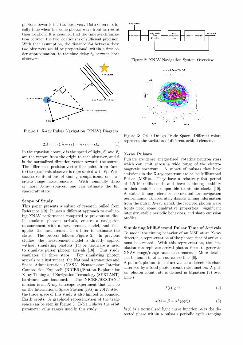
photons towards the two observers. Both observers lo-cally time when the same photon wave front arrives attheir location. It is assumed that the time synchroniza-tion between the two locations is of sufficient precision.With that assumption, the distance ∆d between thesetwo observers would be proportional, within a first or-der approximation, to the time delay td between bothobservers.

Figure 1: X-ray Pulsar Navigation (XNAV) Diagram

∆d = n · (~r2 − ~r1) = n · ~r3 = ctd (1)

In the equation above, c is the speed of light, ~r1 and ~r2

are the vectors from the origin to each observer, and nis the normalized direction vector towards the source.The differenced position vector that points from Earthto the spacecraft observer is represented with ~r3. Withsuccessive iterations of timing comparisons, one cancreate range measurements. With nominally threeor more X-ray sources, one can estimate the fullspacecraft state.

Scope of StudyThis paper presents a subset of research pulled fromReference [19]. It uses a different approach to evaluat-ing XNAV performance compared to previous studies.It simulates photons arrivals, creates a navigationmeasurement with a measurement model, and thenapplies the measurement in a filter to estimate thestate. The process follows Figure 2. In previousstudies, the measurement model is directly appliedwithout simulating photons [14] or hardware is usedto simulate pulsar photon arrivals [18]. This studysimulates all three steps. For simulating photonarrivals to a instrument, the National Aeronautics andSpace Administration (NASA) Neutron-star InteriorComposition ExploreR (NICER)/Station Explorer forX-ray Timing and Navigation Technology (SEXTANT)hardware was baselined. The NICER/SEXTANTmission is an X-ray telescope experiment that will beon the International Space Station (ISS) in 2017. Also,the trade space of this study is also limited to boundedEarth orbits. A graphical representation of the tradespace can be seen in Figure 3. Table 1 shows the orbitparameter value ranges used in this study.

Figure 2: XNAV Navigation System Overview

Figure 3: Orbit Design Trade Space. Different colorsrepresent the variation of different orbital elements.

X-ray PulsarsPulsars are dense, magnetized, rotating neutron starswhich can emit across a wide range of the electro-magnetic spectrum. A subset of pulsars that haveemissions in the X-ray spectrum are called MillisecondPulsar (MSP)s. They have a relatively fast periodof 1.5-16 milliseconds and have a timing stabilityin their emissions comparable to atomic clocks [10].A stable timing reference is essential for navigationperformance. To accurately discern timing informationfrom the pulsar X-ray signal, the received photon wavefronts need some qualitative properties: significantintensity, stable periodic behaviors, and sharp emissionprofiles.

Simulating Milli-Second Pulsar Time of ArrivalsTo model the timing behavior of an MSP at an X-raydetector, a representation of the photon time of arrivalsmust be created. With this representation, the sim-ulation can replicate arrival photon times to generateXNAV range/range rate measurements. More detailscan be found in other sources such as [6].A pulsar’s photon time of arrivals at a detector is char-acterized by a total photon count rate function. A pul-sar photon count rate is defined in Equation (3) overtime t.

λ(t) ≥ 0 (2)

λ(t) = β + αh(φ(t)) (3)

h(φ) is a normalized light curve function, φ is the de-tected phase within a pulsar’s periodic cycle (ranging

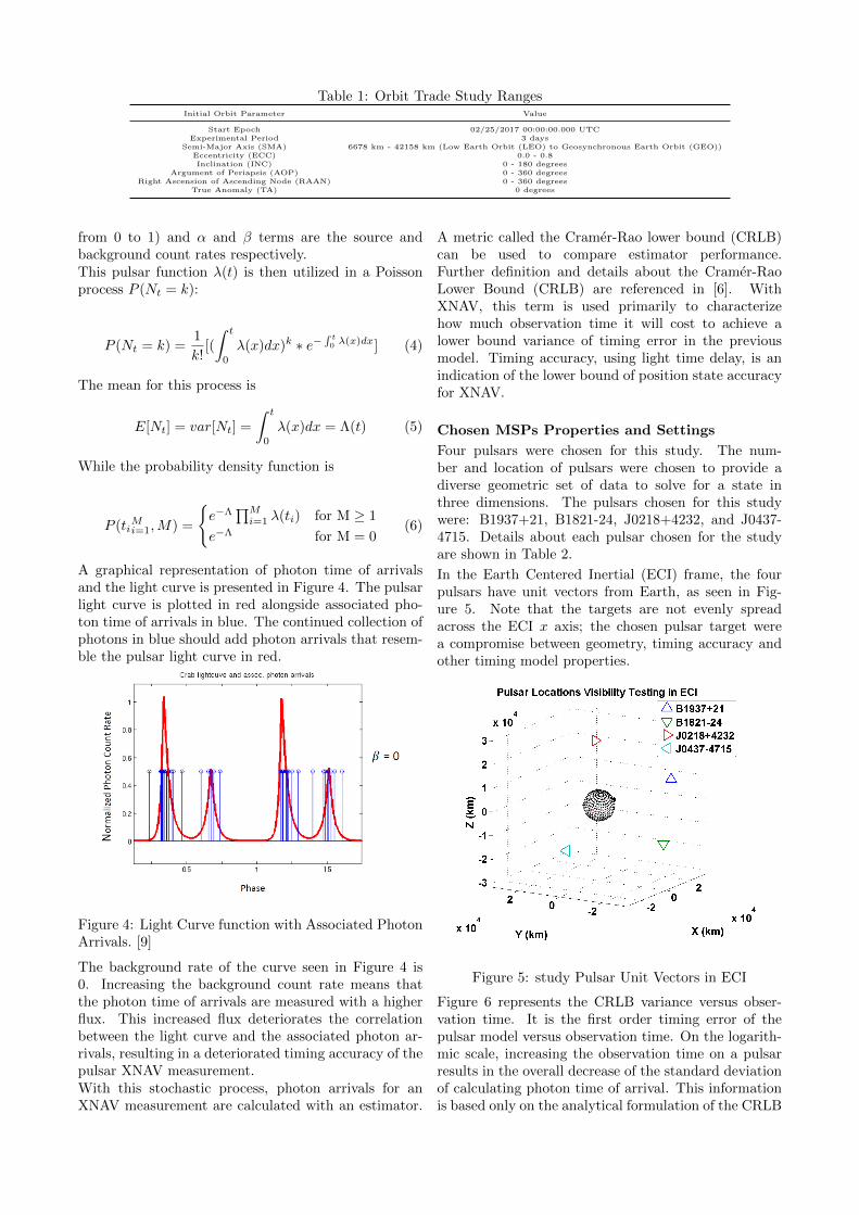
Table 1: Orbit Trade Study RangesInitial Orbit Parameter Value

Start Epoch 02/25/2017 00:00:00.000 UTCExperimental Period 3 days

Semi-Major Axis (SMA) 6678 km - 42158 km (Low Earth Orbit (LEO) to Geosynchronous Earth Orbit (GEO))Eccentricity (ECC) 0.0 - 0.8Inclination (INC) 0 - 180 degrees

Argument of Periapsis (AOP) 0 - 360 degreesRight Ascension of Ascending Node (RAAN) 0 - 360 degrees

True Anomaly (TA) 0 degrees

from 0 to 1) and α and β terms are the source andbackground count rates respectively.This pulsar function λ(t) is then utilized in a Poissonprocess P (Nt = k):

P (Nt = k) =1

k![(

∫ t

0

λ(x)dx)k ∗ e−∫ t0λ(x)dx] (4)

The mean for this process is

E[Nt] = var[Nt] =

∫ t

0

λ(x)dx = Λ(t) (5)

While the probability density function is

P (tiMi=1,M) =

{e−Λ

∏Mi=1 λ(ti) for M ≥ 1

e−Λ for M = 0(6)

A graphical representation of photon time of arrivalsand the light curve is presented in Figure 4. The pulsarlight curve is plotted in red alongside associated pho-ton time of arrivals in blue. The continued collection ofphotons in blue should add photon arrivals that resem-ble the pulsar light curve in red.

Figure 4: Light Curve function with Associated PhotonArrivals. [9]

The background rate of the curve seen in Figure 4 is0. Increasing the background count rate means thatthe photon time of arrivals are measured with a higherflux. This increased flux deteriorates the correlationbetween the light curve and the associated photon ar-rivals, resulting in a deteriorated timing accuracy of thepulsar XNAV measurement.With this stochastic process, photon arrivals for anXNAV measurement are calculated with an estimator.

A metric called the Cramer-Rao lower bound (CRLB)can be used to compare estimator performance.Further definition and details about the Cramer-RaoLower Bound (CRLB) are referenced in [6]. WithXNAV, this term is used primarily to characterizehow much observation time it will cost to achieve alower bound variance of timing error in the previousmodel. Timing accuracy, using light time delay, is anindication of the lower bound of position state accuracyfor XNAV.

Chosen MSPs Properties and Settings

Four pulsars were chosen for this study. The num-ber and location of pulsars were chosen to provide adiverse geometric set of data to solve for a state inthree dimensions. The pulsars chosen for this studywere: B1937+21, B1821-24, J0218+4232, and J0437-4715. Details about each pulsar chosen for the studyare shown in Table 2.

In the Earth Centered Inertial (ECI) frame, the fourpulsars have unit vectors from Earth, as seen in Fig-ure 5. Note that the targets are not evenly spreadacross the ECI x axis; the chosen pulsar target werea compromise between geometry, timing accuracy andother timing model properties.

Figure 5: study Pulsar Unit Vectors in ECI

Figure 6 represents the CRLB variance versus obser-vation time. It is the first order timing error of thepulsar model versus observation time. On the logarith-mic scale, increasing the observation time on a pulsarresults in the overall decrease of the standard deviationof calculating photon time of arrival. This informationis based only on the analytical formulation of the CRLB

Table 2: List of Study MSP Pulsars for Navigation [18]Name Period Source Pulsed Rate Total Bkg Rate TOA & Models Timing Accuracy Obs Time/Meas

(ms) (α, cnts/s) (β, cnts/s) Source (s) (s)

B1937+21 1.558 0.029 0.24 PPTA 1.40e-5 1800B1821-24 3.054 0.093 0.22 PPTA/Nancay 1.64e-5 600

J0218+4232 2.323 0.082 0.20 Nancay 6.4e-5 900J0437-4715 5.757 0.283 0.62 PPTA 2e-4 600

and does not include hardware impacts.

Figure 6: Source pulsars chosen and CRLB observationtime

It is important to note that any point along eachplot in Figure 6 can be chosen to dynamically adjusttiming accuracy for navigation performance. Thisstudy fixes that value with two bounds. A lower boundof observation time was made based on providing aminimal 2e-5 second timing accuracy(an equivalent toabout 5 km of position state accuracy). On the otherside, observations of each pulsar were capped based onthe orbital period of the trade space. Within the tradespace, the smallest value of SMA equates to an orbitalperiod of 5400 seconds. This value was the maximumobservation time upper bound. With both the verticaland horizontal axis bounded, each pulsar’s observationtime per measurement was chosen. See Table 2 forthe direct values. These values are also representedgraphically by the black dots in Figure 6. Finally, theoptimization process to batch and allocate photon timeof arrivals and the measurement model were based onthe formulations in references [14] and [18]. This studydirectly utilizies those formulations to translate photontime of arrivals into XNAV measurements.

Orbit and Navigation

The orbit design and navigation setup for this studywas designed to characterize one to one a large subsetof bounded Earth orbits. In order to do so, this sectiondefines the orbit trade space, the force models, and thesetup of the navigation filter.

The orbit force model in this study includes the con-servative forces of Earth oblateness and point gravity.They and other spacecraft parameters for the study arelisted in Table 3 and were used to propagate the space-craft dynamics in the estimate and truth state:

An Extended Kalman Filter (EKF) was implementedto determine the predictive and definitive accuracy of

the resultant orbit determination. For this study, theEKF measurement noise matrix R is directly definedby a metric called the Cramer-Rao lower bound. Nomi-nally, the process noise matrix Q would also need to beadjusted for each orbit design. This study does not im-plement the process noise matrix in this way. Instead,a series of assumptions were made in order to equallycharacterize the trade space:

1. The process noise matrix Q is zeroed out.

2. The truth and estimate state force models are thesame, with two body forces and the same order ofhigher order geopotential gravity terms.

3. The same initial state offset of 1 km SMA was madebetween the initial truth and estimate state.

4. The covariance initial state is set to bound the ini-tial state offset.

Items 1 and 2 by themselves would make any navigationirrelevant, as the estimate state’s dynamics on boardthe spacecraft would always match the truth state for alltime. Item 3 ensures error growth between the estimateand the truth. With items 2 and 3, the filter will beforced to use XNAV measurements over the estimatepropagator. Item 4 ensures that the filter will recognizea need to make a correction. With these four items, thefilter relies purely on XNAV measurements for any stateestimation convergence.

Figure 7: Navigation performance at a 300 km altitudecircular orbit with no applied measurements

As seen in Figure 7, a scenario that does not applyany XNAV measurements will deteriorate. The blueline indicates the actual error between truth/estimatestates while the red line indicates the filter’s knowledgeof that error within the covariance. As the covariancecarries the variance of both position and velocity inits diagonal, the red line represents the 3σ covariance

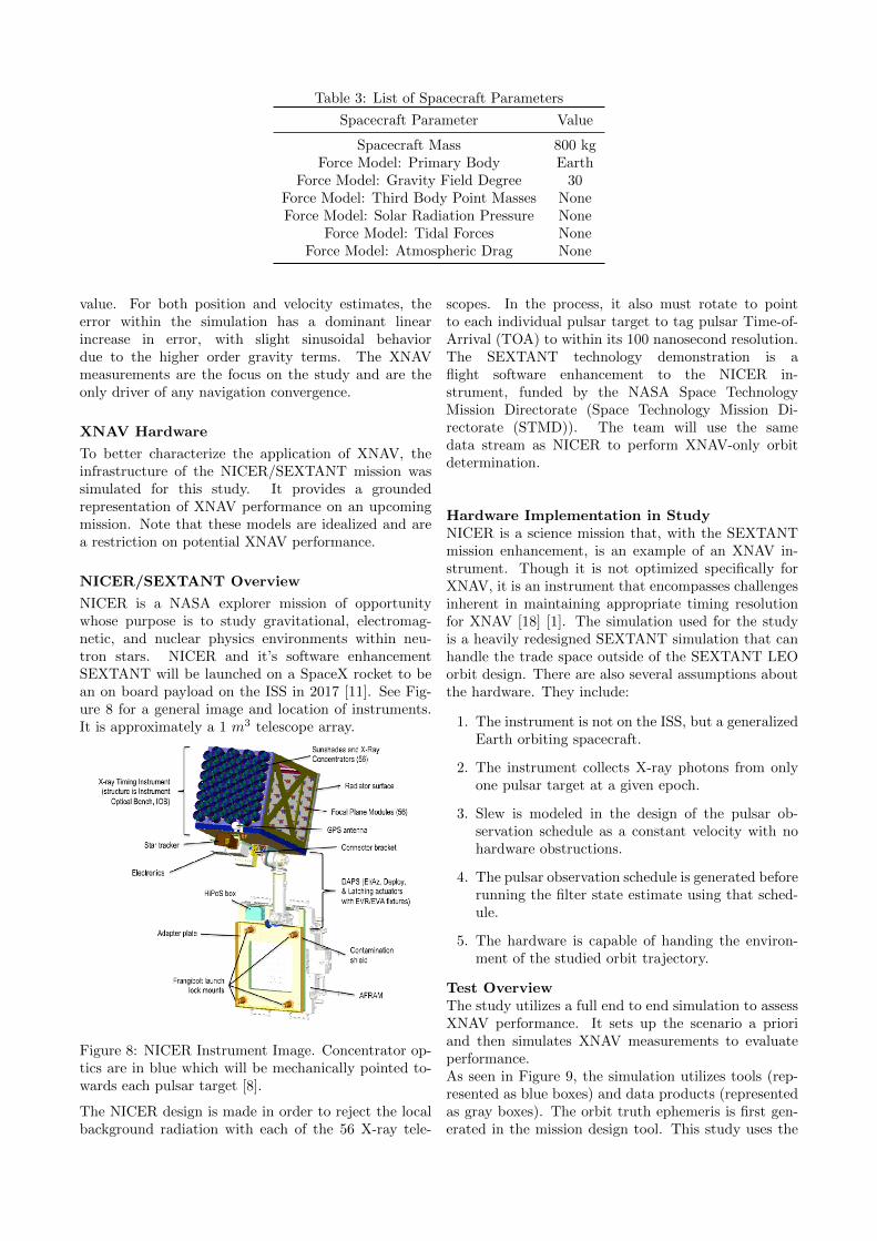
Table 3: List of Spacecraft Parameters

Spacecraft Parameter Value

Spacecraft Mass 800 kgForce Model: Primary Body Earth

Force Model: Gravity Field Degree 30Force Model: Third Body Point Masses NoneForce Model: Solar Radiation Pressure None

Force Model: Tidal Forces NoneForce Model: Atmospheric Drag None

value. For both position and velocity estimates, theerror within the simulation has a dominant linearincrease in error, with slight sinusoidal behaviordue to the higher order gravity terms. The XNAVmeasurements are the focus on the study and are theonly driver of any navigation convergence.

XNAV Hardware

To better characterize the application of XNAV, theinfrastructure of the NICER/SEXTANT mission wassimulated for this study. It provides a groundedrepresentation of XNAV performance on an upcomingmission. Note that these models are idealized and area restriction on potential XNAV performance.

NICER/SEXTANT Overview

NICER is a NASA explorer mission of opportunitywhose purpose is to study gravitational, electromag-netic, and nuclear physics environments within neu-tron stars. NICER and it’s software enhancementSEXTANT will be launched on a SpaceX rocket to bean on board payload on the ISS in 2017 [11]. See Fig-ure 8 for a general image and location of instruments.It is approximately a 1 m3 telescope array.

Figure 8: NICER Instrument Image. Concentrator op-tics are in blue which will be mechanically pointed to-wards each pulsar target [8].

The NICER design is made in order to reject the localbackground radiation with each of the 56 X-ray tele-

scopes. In the process, it also must rotate to pointto each individual pulsar target to tag pulsar Time-of-Arrival (TOA) to within its 100 nanosecond resolution.The SEXTANT technology demonstration is aflight software enhancement to the NICER in-strument, funded by the NASA Space TechnologyMission Directorate (Space Technology Mission Di-rectorate (STMD)). The team will use the samedata stream as NICER to perform XNAV-only orbitdetermination.

Hardware Implementation in StudyNICER is a science mission that, with the SEXTANTmission enhancement, is an example of an XNAV in-strument. Though it is not optimized specifically forXNAV, it is an instrument that encompasses challengesinherent in maintaining appropriate timing resolutionfor XNAV [18] [1]. The simulation used for the studyis a heavily redesigned SEXTANT simulation that canhandle the trade space outside of the SEXTANT LEOorbit design. There are also several assumptions aboutthe hardware. They include:

1. The instrument is not on the ISS, but a generalizedEarth orbiting spacecraft.

2. The instrument collects X-ray photons from onlyone pulsar target at a given epoch.

3. Slew is modeled in the design of the pulsar ob-servation schedule as a constant velocity with nohardware obstructions.

4. The pulsar observation schedule is generated beforerunning the filter state estimate using that sched-ule.

5. The hardware is capable of handing the environ-ment of the studied orbit trajectory.

Test OverviewThe study utilizes a full end to end simulation to assessXNAV performance. It sets up the scenario a prioriand then simulates XNAV measurements to evaluateperformance.As seen in Figure 9, the simulation utilizes tools (rep-resented as blue boxes) and data products (representedas gray boxes). The orbit truth ephemeris is first gen-erated in the mission design tool. This study uses the

Figure 9: Simulation Infrastructure [17]

NASA open source orbit propagation software calledGeneral Mission Analysis Tool (GMAT). Using theephemeris, the pulse phase models block extrapolatespulsar information from a database using open sourcesoftware called TEMPO2 [5]. The background radia-tion environment throughout the projected spacecrafttrajectory is also calculated in this section. At the sametime, internal software is used to calculate pulsar visi-bility and generate an observation schedule. Once theorbit design/pulsar phase model products are produced,the simulation runs the XNAV measurement process tosimulate photon events and create measurements. Themeasurements are applied to a running EKF and thenavigation performance is recorded.

Designed for this study, software algorithms that arecritical to an Earth orbit trade space design are furtherexplored in the following sections. These include thevisibility models, the background radiation model, andthe scheduling algorithm that optimizes navigationperformance.

Pulsar Visibility

An XNAV measurement is based on collecting photonTOAs. This process requires an observation time oneach pulsar based on the CRLB. Due to the significantobservation time, the XNAV process is subject to physi-cal blockages between the detector and the pulsar. Thisstudy checks for occultations for each ephemeris timestep from celestial occultations and from areas with ex-treme background radiation.

The driving occultations are from celestial bodies. Thisstudy models occultations from the Sun, Earth, andMoon. See Figure 10.

The other area of occultation applied in this studywere areas with highly variable background radiation.Areas with too variable of a background rate in thespacecraft’s immediate area were considered occulted.The South Atlantic Anomaly (SAA) at orbit altitudesaround 300-1000 km as well as areas around the mag-netic north and south poles have this variation in back-ground radiation(see Figure 11).

To avoid these areas, the SAA and areas around the

Figure 10: Celestial Body Occultation Model

Figure 11: Background Radiation Environment around400 km altitude versus Geodetic Longitude/Latitude(degrees). Note the high concentration areas aroundthe South Atlantic as well as the magnetic poles [12].

magnetic poles are restricted by a longitude/latitudebox. Restricts were applied at orbit altitudes between300-1000 km, while the magnetic pole areas wereenforced for any orbit altitude. With these back-ground occultations, all the pulsars were consideredocculted when the spacecraft orbit enters these regions.The geometry used for these structures comes fromthe National Oceanic and Atmospheric Administra-tion (NOAA) geomagnetic map reference [4] [13].Other areas around Earth were scaled in backgroundradiation, detailed in the next section.

Background Radiation Environment

The Earth’s background radiation environment consistsof two dominating radiation structures around Earthcalled the Van Allen belts. They are two bands of highenergy levels that exist within 10 Earth radii from theEarth’s center [15].

Figure 12: Background Radiation Electron Environ-ment from the Earth surface to 7 Earth Radii. Heatplot is scaled for electron flux greater than 1 MeV. UsesData from the AE-8 model at solar maximum [7].

As seen with this high energy map in Figure 12, two ar-eas between 1-2 Earth radii and 3-5 Earth radii have sig-nificantly higher concentrations of electrons than otherareas. With the significant variation in background en-vironment, this study models the background environ-ment based on the primary Van Allen Belt structures.See Figure 13 for a logarithmic plot used in the study.The horizontal axis is the spacecraft altitude at theequator in Earth radii, while the vertical axis representsthe AE-8 model of electron flux at solar maximum thatis greater than 100 MeV per centimeter squared sec-onds. A reference electron flux is marked in the simu-lation at 0.1 Earth radii. The other values on the plotare scaled relative to the flux at that value. For a givenspacecraft state, a corresponding amount of backgroundradiation is applied to the photon simulation and navi-gation measurement generation.

This application makes the assumption that thehardware will be able to handle these environments.The hardware will provide appropriate backgroundrejection in order to effectively detect X-ray photonarrivals from individual MSP sources. One hardwareexample to encourage background rejection is tofocus the X-ray detector on one pulsar at a time.The consequences of this assumption means that anobservation schedule must be produced a priori.

Pulsar Observation Scheduling

In order to receive pulsar X-ray photons, observationsof individual pulsars need to be prioritized. It takes asignificant period of observation time to make a navi-gation measurement, so scheduled observations must beevaluated to ensure that they are effective for XNAV.With the hardware assumptions built into this study,this also requires that one pulsar is observed at a time

Figure 13: Background Radiation Electron Environ-ment versus Distance from Earth. Uses Data from theAE-8 model at solar maximum [16].

and that the schedule is produced before the EKF solu-tion is simulated. To address these issues, a schedulingalgorithm was designed for this study.

The schedule algorithm builds a schedule by append-ing immediate observation schedules to a final scheduleproduct. It creates multiple immediate schedules thatcomprise of a subset of the full simulation period. Itthen evaluates their metric and chooses the ideal sched-ule. This continues until the end of the simulation pe-riod.

An immediate schedule is created by traversing for-ward in time through both visibility and ephemerisdata, scheduling pulsar observations focused on mak-ing a measurement for a particular pulsar. Multiplepossible schedules are created in the process; for N pul-sars, there are N immediate schedules. Observationsare scheduled up until an XNAV measurement on thatpulsar can be created, based on the the CRLB analysisdescribed earlier. If that chosen pulsar is occulted butmore observation time is required, the pulsar with thesmallest observation time based on the CRLB is choseninstead for observation.

Once these immediate schedules are produced, thescheduling algorithm then uses a local greedy heuris-tic to pick a schedule to append to the final observa-tion schedule. That schedule is chosen using a covari-ance based analysis. Looping through each immediateschedule, the algorithm calculates (or initializes) the co-variance matrix (P−

i ), the state transition matrix (Φ),and the spacecraft state at the current simulation timet0. Next, the previous covariance Pi−1 is then propa-gated up to the first measurement time made from animmediate schedule called ti.

P−i = Φ(t0, ti)Pi−1Φ(t0, ti)

T (7)

Once the covariance is propagated to the measurementtime (P−

i ), a Kalman gain is updated based on the co-variance. This also uses the relevant measurement noise

from the pulsar Ri.

Ki = P−i H

Ti [HiP

−i H

Ti +Ri] (8)

The covariance is then updated with the given measure-ment.

Pi = [I −KiHi]P−i (9)

If more than one measurement was made with the im-mediate schedule, the process is repeated. The algo-rithm then evaluates a metric based on the covariancematrix to determine which schedule to choose. Based onpast research [3] [2], the criteria of this scheduling algo-rithm is to minimize the projected SMA variance. Thisis done with a partially differentiated vis viva equation(Equation (10)) with respect to position magnitude rand velocity magnitude v. As reference, the formula-tion is listed below:

−µ2a

=1

2v2 − µ

r(10)

δr =1

2

[(2µ− rv2)2

µ2

]δa (11)

δv =1

2

[(2µ− rv2)2

µr2v

]δa (12)

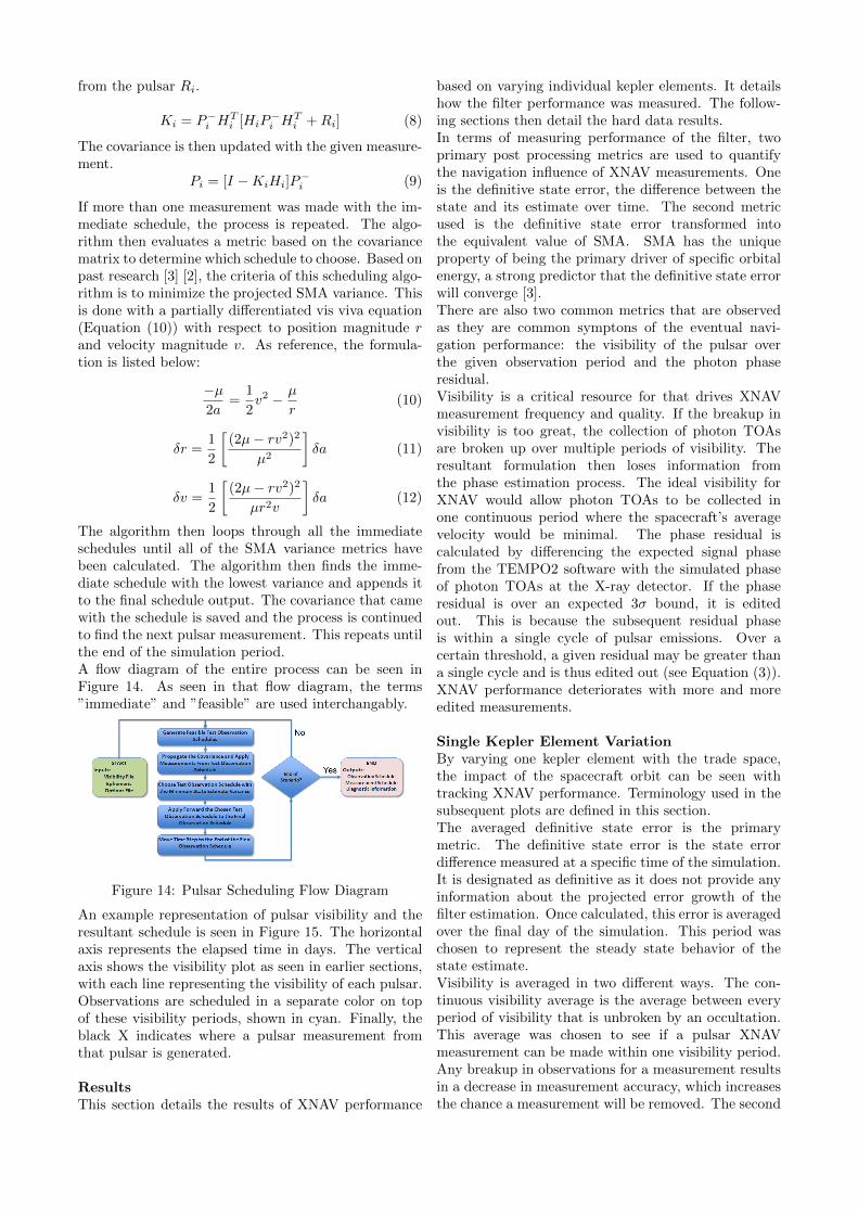
The algorithm then loops through all the immediateschedules until all of the SMA variance metrics havebeen calculated. The algorithm then finds the imme-diate schedule with the lowest variance and appends itto the final schedule output. The covariance that camewith the schedule is saved and the process is continuedto find the next pulsar measurement. This repeats untilthe end of the simulation period.A flow diagram of the entire process can be seen inFigure 14. As seen in that flow diagram, the terms”immediate” and ”feasible” are used interchangably.

Figure 14: Pulsar Scheduling Flow Diagram

An example representation of pulsar visibility and theresultant schedule is seen in Figure 15. The horizontalaxis represents the elapsed time in days. The verticalaxis shows the visibility plot as seen in earlier sections,with each line representing the visibility of each pulsar.Observations are scheduled in a separate color on topof these visibility periods, shown in cyan. Finally, theblack X indicates where a pulsar measurement fromthat pulsar is generated.

ResultsThis section details the results of XNAV performance

based on varying individual kepler elements. It detailshow the filter performance was measured. The follow-ing sections then detail the hard data results.In terms of measuring performance of the filter, twoprimary post processing metrics are used to quantifythe navigation influence of XNAV measurements. Oneis the definitive state error, the difference between thestate and its estimate over time. The second metricused is the definitive state error transformed intothe equivalent value of SMA. SMA has the uniqueproperty of being the primary driver of specific orbitalenergy, a strong predictor that the definitive state errorwill converge [3].There are also two common metrics that are observedas they are common symptons of the eventual navi-gation performance: the visibility of the pulsar overthe given observation period and the photon phaseresidual.Visibility is a critical resource for that drives XNAVmeasurement frequency and quality. If the breakup invisibility is too great, the collection of photon TOAsare broken up over multiple periods of visibility. Theresultant formulation then loses information fromthe phase estimation process. The ideal visibility forXNAV would allow photon TOAs to be collected inone continuous period where the spacecraft’s averagevelocity would be minimal. The phase residual iscalculated by differencing the expected signal phasefrom the TEMPO2 software with the simulated phaseof photon TOAs at the X-ray detector. If the phaseresidual is over an expected 3σ bound, it is editedout. This is because the subsequent residual phaseis within a single cycle of pulsar emissions. Over acertain threshold, a given residual may be greater thana single cycle and is thus edited out (see Equation (3)).XNAV performance deteriorates with more and moreedited measurements.

Single Kepler Element VariationBy varying one kepler element with the trade space,the impact of the spacecraft orbit can be seen withtracking XNAV performance. Terminology used in thesubsequent plots are defined in this section.The averaged definitive state error is the primarymetric. The definitive state error is the state errordifference measured at a specific time of the simulation.It is designated as definitive as it does not provide anyinformation about the projected error growth of thefilter estimation. Once calculated, this error is averagedover the final day of the simulation. This period waschosen to represent the steady state behavior of thestate estimate.Visibility is averaged in two different ways. The con-tinuous visibility average is the average between everyperiod of visibility that is unbroken by an occultation.This average was chosen to see if a pulsar XNAVmeasurement can be made within one visibility period.Any breakup in observations for a measurement resultsin a decrease in measurement accuracy, which increasesthe chance a measurement will be removed. The second

Figure 15: Example of a Pulsar Schedule Overlay to a Visibility Plot

visibility average is the average visibility per orbitalperiod. Both summarize the continuity of individualperiods and the frequency they appear relative to theorbit dynamics.Measurement quality is determined by the totalnumber of measurements and percent of measurementsremoved. The total number of measurements is thetotal number of measurements that were generatedin the simulation. The percentage of measurementsremoved records the ratio of rejected over total mea-surements due to the phase residual limits. Bothnumbers are needed to determine the total number ofXNAV measurements used in the EKF.

Variation of Orbit Semi-Major AxisFigure 16 is a graphical representation of the orbittrade space with SMA. XNAV performance over vary-ing semi-major axis is represented in Figures 17, 18,and 19. The nominal orbit parameters have an eccen-tricity of 0 and an inclination of 0°. As the orbit iscircular and equatorial, argument of periapsis/RAANare not formally defined.

For definitive state error and the definitive statesemi-major axis error, the lowest value in the tradespace of 6678 km semi-major axis had an averageposition error above 5 km and an average velocityerror above 0.005 km/s. The rest of the semi-majoraxis trade space stays below those values. The orbitdesign has the most influence on the lowest value ofsemi-major axis, and averages out for the rest of thetrade space. There is also an increase in the definitiveposition error that peaks in the middle of the tradespace ( 25000 km semi-major axis).

The measurement quality can be seen in Figure 18.A peak percentage of measurements (around 30%)are edited out around an semi-major axis of 25000

Figure 16: SMA Orbit Trade Space. Orbit trade valueincreases from blue (6678 km) to red (42158 km) foreach trajectory.

km, just like the peak in state error averages. Thenumber of measurements increases with semi-majoraxis until a value of 300 measurements around 20,000km semi-major axis. At this point, the total number ofmeasurements remains +/- 50 measurements off thatnominal value for the rest of the trade space.Finally, increasing semi-major axis increases visibilityof all pulsars. With increasing semi-major axis,each pulsar increases visibility at a different linearslope. With the geometry seen in Figure 16, pulsarJ0437-4715 always has visibility on the spacecraft aftera certain threshold of semi-major axis. The visibilityfor that pulsar peaks at about 4320 minutes, or the fullsimulation time of three days.The increase of semi-major axis significantly increasesthe visibility of all pulsars. The increase in visibility

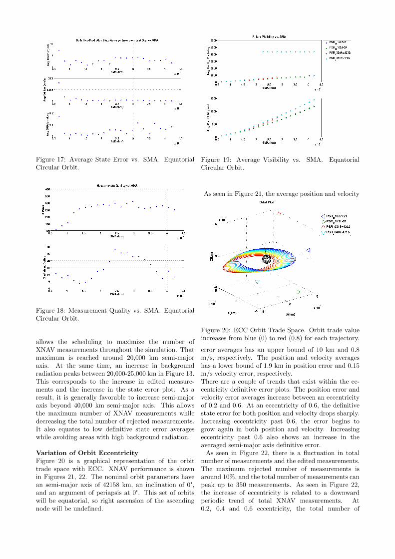
Figure 17: Average State Error vs. SMA. EquatorialCircular Orbit.

Figure 18: Measurement Quality vs. SMA. EquatorialCircular Orbit.

allows the scheduling to maximize the number ofXNAV measurements throughout the simulation. Thatmaximum is reached around 20,000 km semi-majoraxis. At the same time, an increase in backgroundradiation peaks between 20,000-25,000 km in Figure 13.This corresponds to the increase in edited measure-ments and the increase in the state error plot. As aresult, it is generally favorable to increase semi-majoraxis beyond 40,000 km semi-major axis. This allowsthe maximum number of XNAV measurements whiledecreasing the total number of rejected measurements.It also equates to low definitive state error averageswhile avoiding areas with high background radiation.

Variation of Orbit EccentricityFigure 20 is a graphical representation of the orbittrade space with ECC. XNAV performance is shownin Figures 21, 22. The nominal orbit parameters havean semi-major axis of 42158 km, an inclination of 0°,and an argument of periapsis at 0°. This set of orbitswill be equatorial, so right ascension of the ascendingnode will be undefined.

Figure 19: Average Visibility vs. SMA. EquatorialCircular Orbit.

As seen in Figure 21, the average position and velocity

Figure 20: ECC Orbit Trade Space. Orbit trade valueincreases from blue (0) to red (0.8) for each trajectory.

error averages has an upper bound of 10 km and 0.8m/s, respectively. The position and velocity averageshas a lower bound of 1.9 km in position error and 0.15m/s velocity error, respectively.There are a couple of trends that exist within the ec-centricity definitive error plots. The position error andvelocity error averages increase between an eccentricityof 0.2 and 0.6. At an eccentricity of 0.6, the definitivestate error for both position and velocity drops sharply.Increasing eccentricity past 0.6, the error begins togrow again in both position and velocity. Increasingeccentricity past 0.6 also shows an increase in theaveraged semi-major axis definitive error.

As seen in Figure 22, there is a fluctuation in totalnumber of measurements and the edited measurements.The maximum rejected number of measurements isaround 10%, and the total number of measurements canpeak up to 350 measurements. As seen in Figure 22,the increase of eccentricity is related to a downwardperiodic trend of total XNAV measurements. At0.2, 0.4 and 0.6 eccentricity, the total number of

Figure 21: Average State Error vs. ECC. 42158 kmsemi-major axis Equatorial Orbit.

Figure 22: Measurement Quality vs. ECC. 42158 kmSMA Equatorial Orbit.

measurements reaches a local minimum. At the sametime, increases in edited measurements occur between0.2-0.3 eccentricity and after 0.5 eccentricity. Together,the total number of used XNAV measurements peaksbetween 0.1 and 0.2 eccentricity, while the othervalues of eccentricity show a drop in used XNAVmeasurements.

Seen in Figure 23, visibility has a significant dropbetween values of 0.1 and 0.6. The visibility averagesdouble in value beyond 0.6 eccentricity.In summary, an eccentricity up to 0.2 has someminor benefits to XNAV performance. Increasingeccentricity shows an increase in visibility and totalmeasurements while decreasing rejected measurements.Even though the definitive average error in position,velocity, and semi-major axis stay at a lower valueup to 0.2 eccentricity, the pulsar visibility and totalnumber of measurements drop between 0.1 and 0.2eccentricity. Beyond 0.2 eccentricity, a growth indefinitive state error is observed. The return of pulsarJ0437-4715 visibility at an eccentricity of 0.6 equatesto the sudden jump in total measurements and thusdefinitive average error. Increasing eccentricity past

Figure 23: Average Visibility vs. ECC. 42158 km SMAEquatorial Orbit.

0.6 decreases the total measurements and the numberof rejected measurements, which brings up all theaverages of definitive state error.

Variation of Orbit InclinationFigure 24 is a graphical representation of the orbittrade space with INC. XNAV performance over varyinginclination is shown in Figures 25, 26, and 27. Thenominal orbit parameters have an semi-major axis of42158 km, an eccentricity of 0, and a right ascensionof the ascending node at 0°. argument of periapsis isundefined for a circular orbit.

The variation of inclination shows an averaged state

Figure 24: INC Orbit Trade Space. Orbit trade valueincreases from blue (0°) to red (180°) for each trajectory.

error below 6 km Root Sum Square (RSS) in position,4.2e-4 km/s in velocity, and 0.4 km for SMA estimationfor the entire trade space. There is a maximum averagestate error in all plots of Figure 25 near 90° INC.

There is a drop in total measurements and anpercentage increase in edited measurements around90° INC, as seen in Figure 26.The visibility averaged periods between an inclination

of 60°and 160° suddenly drops for continuous periodsbut not for orbital periods. Also, pulsar J0427-4715is visible for the entire three day scenario between aninclination of 25° and 50°.

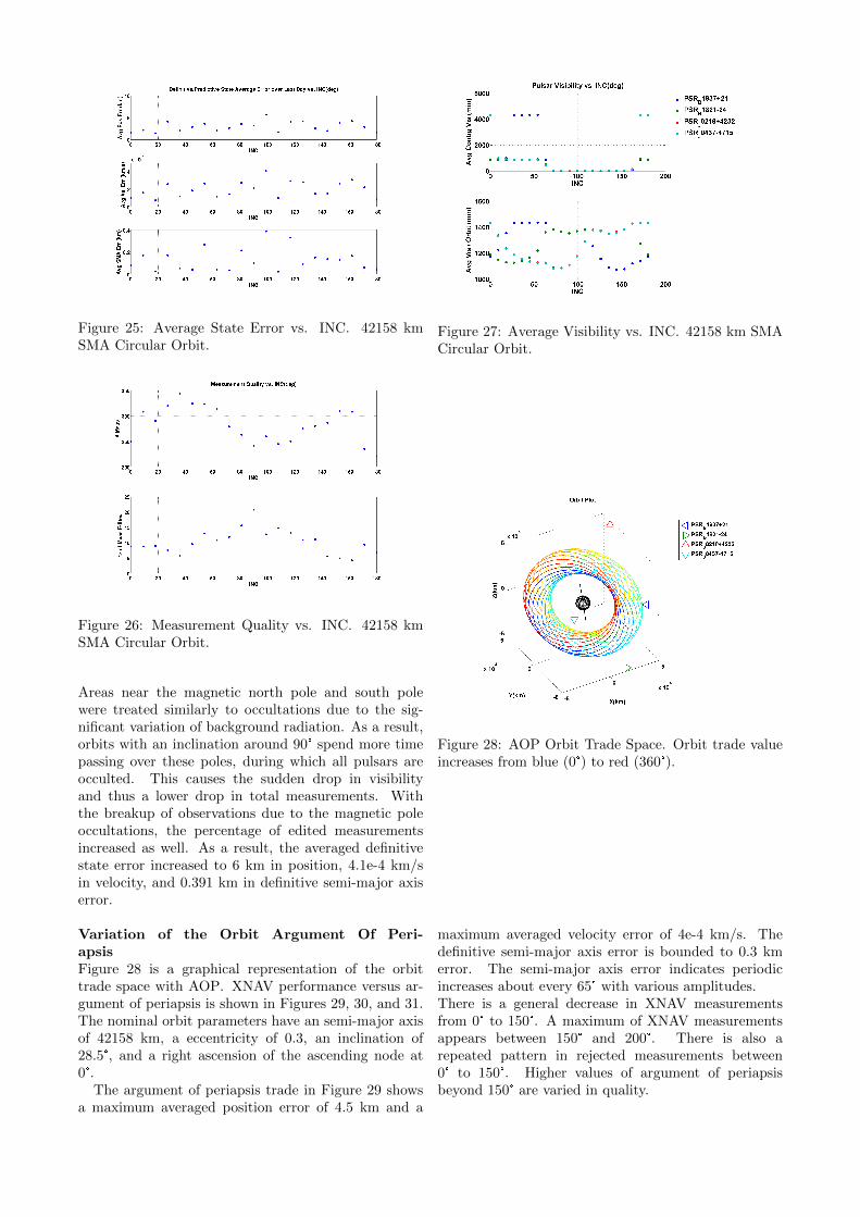
Figure 25: Average State Error vs. INC. 42158 kmSMA Circular Orbit.

Figure 26: Measurement Quality vs. INC. 42158 kmSMA Circular Orbit.

Areas near the magnetic north pole and south polewere treated similarly to occultations due to the sig-nificant variation of background radiation. As a result,orbits with an inclination around 90° spend more timepassing over these poles, during which all pulsars areocculted. This causes the sudden drop in visibilityand thus a lower drop in total measurements. Withthe breakup of observations due to the magnetic poleoccultations, the percentage of edited measurementsincreased as well. As a result, the averaged definitivestate error increased to 6 km in position, 4.1e-4 km/sin velocity, and 0.391 km in definitive semi-major axiserror.

Variation of the Orbit Argument Of Peri-apsisFigure 28 is a graphical representation of the orbittrade space with AOP. XNAV performance versus ar-gument of periapsis is shown in Figures 29, 30, and 31.The nominal orbit parameters have an semi-major axisof 42158 km, a eccentricity of 0.3, an inclination of28.5°, and a right ascension of the ascending node at0°.

The argument of periapsis trade in Figure 29 showsa maximum averaged position error of 4.5 km and a

Figure 27: Average Visibility vs. INC. 42158 km SMACircular Orbit.

Figure 28: AOP Orbit Trade Space. Orbit trade valueincreases from blue (0°) to red (360°).

maximum averaged velocity error of 4e-4 km/s. Thedefinitive semi-major axis error is bounded to 0.3 kmerror. The semi-major axis error indicates periodicincreases about every 65° with various amplitudes.There is a general decrease in XNAV measurementsfrom 0° to 150°. A maximum of XNAV measurementsappears between 150° and 200°. There is also arepeated pattern in rejected measurements between0° to 150°. Higher values of argument of periapsisbeyond 150° are varied in quality.

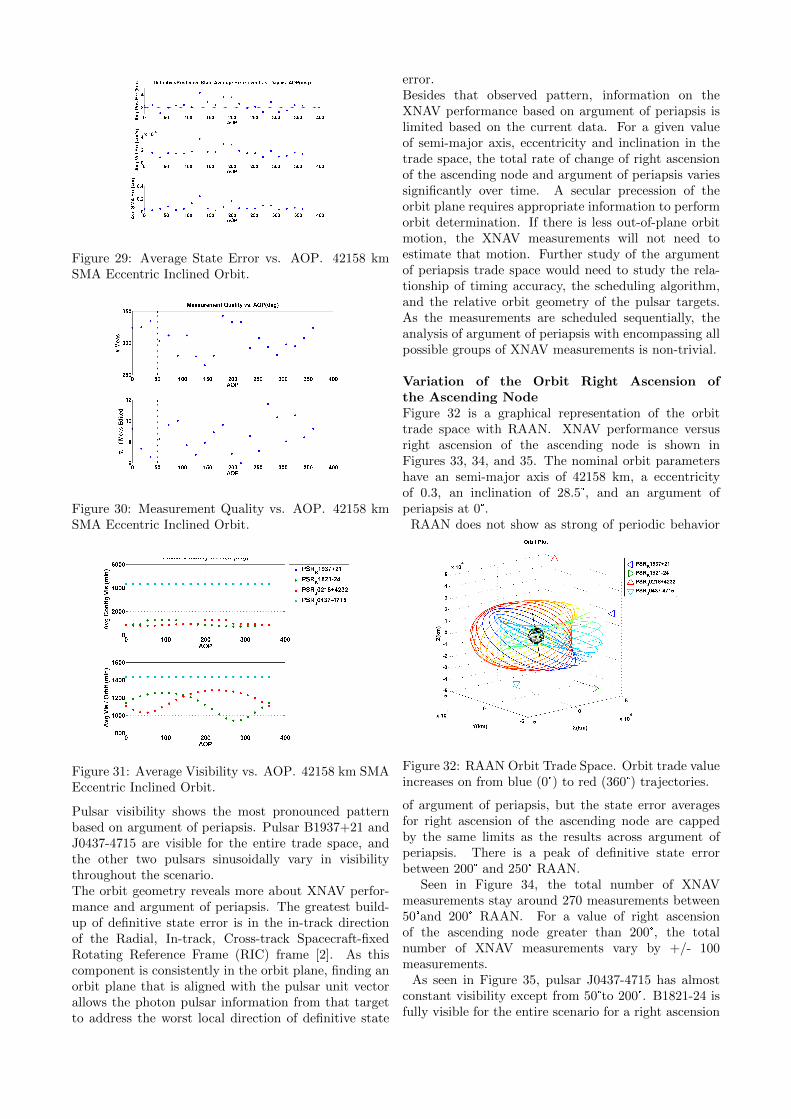
Figure 29: Average State Error vs. AOP. 42158 kmSMA Eccentric Inclined Orbit.

Figure 30: Measurement Quality vs. AOP. 42158 kmSMA Eccentric Inclined Orbit.

Figure 31: Average Visibility vs. AOP. 42158 km SMAEccentric Inclined Orbit.

Pulsar visibility shows the most pronounced patternbased on argument of periapsis. Pulsar B1937+21 andJ0437-4715 are visible for the entire trade space, andthe other two pulsars sinusoidally vary in visibilitythroughout the scenario.The orbit geometry reveals more about XNAV perfor-mance and argument of periapsis. The greatest build-up of definitive state error is in the in-track directionof the Radial, In-track, Cross-track Spacecraft-fixedRotating Reference Frame (RIC) frame [2]. As thiscomponent is consistently in the orbit plane, finding anorbit plane that is aligned with the pulsar unit vectorallows the photon pulsar information from that targetto address the worst local direction of definitive state

error.Besides that observed pattern, information on theXNAV performance based on argument of periapsis islimited based on the current data. For a given valueof semi-major axis, eccentricity and inclination in thetrade space, the total rate of change of right ascensionof the ascending node and argument of periapsis variessignificantly over time. A secular precession of theorbit plane requires appropriate information to performorbit determination. If there is less out-of-plane orbitmotion, the XNAV measurements will not need toestimate that motion. Further study of the argumentof periapsis trade space would need to study the rela-tionship of timing accuracy, the scheduling algorithm,and the relative orbit geometry of the pulsar targets.As the measurements are scheduled sequentially, theanalysis of argument of periapsis with encompassing allpossible groups of XNAV measurements is non-trivial.

Variation of the Orbit Right Ascension ofthe Ascending NodeFigure 32 is a graphical representation of the orbittrade space with RAAN. XNAV performance versusright ascension of the ascending node is shown inFigures 33, 34, and 35. The nominal orbit parametershave an semi-major axis of 42158 km, a eccentricityof 0.3, an inclination of 28.5°, and an argument ofperiapsis at 0°.

RAAN does not show as strong of periodic behavior

Figure 32: RAAN Orbit Trade Space. Orbit trade valueincreases on from blue (0°) to red (360°) trajectories.

of argument of periapsis, but the state error averagesfor right ascension of the ascending node are cappedby the same limits as the results across argument ofperiapsis. There is a peak of definitive state errorbetween 200° and 250° RAAN.

Seen in Figure 34, the total number of XNAVmeasurements stay around 270 measurements between50°and 200° RAAN. For a value of right ascensionof the ascending node greater than 200°, the totalnumber of XNAV measurements vary by +/- 100measurements.

As seen in Figure 35, pulsar J0437-4715 has almostconstant visibility except from 50°to 200°. B1821-24 isfully visible for the entire scenario for a right ascension

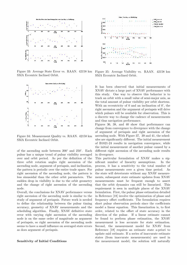
Figure 33: Average State Error vs. RAAN. 42158 kmSMA Eccentric Inclined Orbit.

Figure 34: Measurement Quality vs. RAAN. 42158 kmSMA Eccentric Inclined Orbit.

of the ascending node between 200° and 250°. Eachpulsar has a unique trend of pulsar visibility averagedover and orbit period. As per the definition of thethree orbit rotation angles right ascension of theascending node, argument of periapsis, and inclination,the pattern is periodic over the entire trade space. Forright ascension of the ascending node, the pattern isless sinusoidal than the other orbit parameters. Thesudden drop in visibility is due to the orbit geometryand the change of right ascension of the ascendingnode.Overall, the conclusions for XNAV performance versusright ascension of the ascending node is similar to thestudy of argument of periapsis. Future work is neededto define the relationship between the pulsar timingaccuracy, geometry of XNAV measurements and thescheduling algorithm. Finally, XNAV definitive stateerror with varying right ascension of the ascendingnode is on the same order of magnitude as argumentof periapsis, so right ascension of the ascending nodeseems to have a small influence on averaged state errorsas does argument of periapsis.

Sensitivity of Initial Conditions

Figure 35: Average Visibility vs. RAAN. 42158 kmSMA Eccentric Inclined Orbit.

It has been observed that initial measurements ofXNAV dictate a large part of XNAV performance withthis study. One way to observe this behavior is totrack an orbit with a small value of semi-major axis, asthe total amount of pulsar visibility per orbit shortens.With an eccentricity of 0 and an inclination of 0°, theright ascension and the argument of periapsis will drivewhich pulsars will be available for observation. This isa discrete way to change the cadence of measurementsand thus navigation performance.Figures 36, 38, and 40 show that performance canchange from convergence to divergence with the changeof argument of periapsis and right ascension of theascending node. With Figure 37, 39 and 41, the sched-ules are significantly different. The initial measurementof B1821-24 results in navigation convergence, whilethe initial measurement of another pulsar caused by adifferent right ascension of the ascending node resultsin divergence.This particular formulation of XNAV makes a sig-nificant number of linearity assumptions. In theprocess, it has a sensitivity to the total number ofpulsar measurements over a given time period. Asthe state will deteriorate without any XNAV measure-ments, subsequent state estimate updates from XNAVmeasurements must be frequent enough to assertthat the orbit dynamics can still be linearized. Thisrequirement is seen in multiple places of the XNAVformulation. First, the pulsar phase estimation detailedin Reference [18] involve the optimization of phase andfrequency offset coefficients. The formulation requiresshort pulsar observation periods since the coefficientsmodel a linear equation. This linearization is, to firstorder, related to the offset of state accuracy in thedirection of the pulsar. If a linear estimate cannotbe found to perform phase estimation, the XNAVmeasurement is less accurate for state estimation.Second, the measurement model for XNAV fromReference [18] requires an estimate state a-priori toupdate said estimate. If a series of inaccurate estimatestates (from inaccurate measurements) are used inthe measurement model, the solution will naturally

diverge. Finally, an EKF is formulated by linearizingaround the estimate state. If estimate states in theEKF cannot be related to each other by the lineartransformation of the state transition matrix, the filteritself will also fail to estimate the spacecraft state.

Figure 36: Definitive Error performance for a LEO withan INC of 45°with AOP and RAAN equal to 0°.

Figure 37: Pulsar Visibility/Schedule for a LEO withan INC of 45°with AOP and RAAN equal to 0°.

Conclusions

Initial orbit parameters of closed Earth orbits are an in-dicator of XNAV performance in terms of pulsar avail-ability, the background radiation environment and theresultant spacecraft dynamics. The results of this studyshow a sensitivity of the EKF state estimate perfor-mance based on the resultant cadence of XNAV mea-surements. That cadence is a result of pulsar availabil-ity and the measurement quality, whose behavior is aresult of spacecraft dynamics and ambient backgroundradiation.

The majority of orbits can be tracked with XNAV mea-surements to within no more than 10 km position error,worst direction, in the 3 day experiment period. If theorbit parameters are restricted to a particular subset,this can improve to no more than 5 km position error,worst direction, over 1 day. This section summarizesthe influences that each orbit parameter has on XNAV

Figure 38: Definitive Error performance for a LEO withan INC of 45°, an AOP of 180°and a RAAN of 0°

Figure 39: Pulsar Visibility/Schedule for a LEO withan INC of 45°, an AOP of 180°and a RAAN of 0°

performance. The subsequent section enumerates thediscrete design range suitable for no more than 5 kmposition error, worst direction.

The primary indicators of XNAV performance are SMAand ECC. These orbit parameters will independentlyinfluence pulsar visibility, in-plane orbit dynamics, andthe spacecraft’s ambient background radiation. Thetwo parameters determine the radial distance of thespacecraft from Earth, the value used to define bothbackground radiation as well as occultations due toEarth. The in-plane dynamics of a spacecraft are alsodriven by these two parameters. The specific energy ofan orbit is primarily driven by SMA, while the instan-taneous velocity at a given point on an orbit is drivenby ECC. The INC of an orbit also drives the environ-ment for XNAV measurements as well as the underly-ing spacecraft dynamics. The occulted magnetic poleregions due to the dynamic variation of background ra-diation results in periodic breaks in visibility with or-bits close to +/- 90°inclinations. SMA, ECC, and INCalso influence the non-spherical gravitational accelera-tion J2. In turn, this result modifies the rate of changeof AOP and RAAN, changing the periodic timing ofpulsar visibility/pulsar measurements. Finally, AOPand RAAN complete the orbit definition. Individually,they both drive the initial cadence of XNAV measure-

Figure 40: Definitive Error performance for a LEO withan INC of 45°, an AOP of 0°and a RAAN of 180°

Figure 41: Pulsar Visibility/Schedule for a LEO withan INC of 45°, an AOP of 0°, and a RAAN of 180°

ments, but only minimally so.The results here speak to individual orbital elementvariations. Further reasearch is required in the cou-pled behavior between orbit parameters in order betterunderstand their nature.The study is an extension of previous research bycharacterizing XNAV for tracking generally boundedEarth orbits. Contributions include a model of Earthbackground radiation as well as a novel pulsar ob-servation scheduling algorithm. Both were createdto accommodate for a general bounded Earth orbit.These models help to evaluate the application of XNAVwith similar orbit regimes.

REFERENCES

[1] K.D. Anderson, D.J. Pines, and S.I. Sheikh. Vali-dation of pulsar phase tracking for spacecraft nav-igation. AIAA Journal of Guidance, Control andDynamics, 38 No.10:1885–1897, 2015.

[2] J.R. Carpenter and K.T. Alfriend. Navigationaccuracy guidelines for orbital formation flying.The Journal of the Astronautical Sciences, 53No.2:207–219, 2005.

[3] J.R. Carpenter and E.R. Schiesser. Semimajor axisknowledge and GPS orbit determination. Navi-gation: Journal of the Institute of Navigation, 48No.1:57–68, 2001.

[4] A. Chulliat, S. Macmillian, P. Alken, C. Beg-gan, M. Nair, B. Hamilton, A. Woods, V. Ridley,S. Maus, and A. Thomson. The US/UK worldmagnetic model for 2015-2020: Technical report.National Geophysical Data Center, NOAA.

[5] R. T. Edwards, G. B. Hobbs, and R. N. Manch-ester. TEMPO2, a new pulsar timing package- II. the timing model and precision estimates.Monthly Notices of the Royal Astronomical Soci-ety, 372:1549–1574, November 2006.

[6] A. A. Emadzadeh and J. L. Speyer. Navigation inspace by X-ray pulsars. Springer, 2011.

[7] ESA. ESA Space Environment Information Sys-tem. https://www.spenvis.oma.be/, 2015.

[8] K. C. Gendreau, Z. Arzoumanian, T. Okajima,and the NICER Team. The Neutron-star Inte-rior Composition ExploreR (NICER): an Explorermission of opportunity for soft X-ray timing spec-troscopy. In Space Telescopes and Instrumentation:Ultraviolet to Gamma Ray, volume 8443 of Proc.SPIE. International Society for Optics and Pho-tonics, Sep 2012. doi:10.1117/12.926396.

[9] Jacob M. Hartman and Paul S. Ray. Timing ac-curacy for spin-powered millisecond pulsars: Acomparison of predictions and rxte observations.DARPA XNAV Program Memo, 2005.

[10] John Hartnett and Andre Luiten. Colloquium:Comparison of astrophysical and terrestrial fre-quency standards. Review of Modern Physics,83:1–9, 2011.

[11] Jason W. Mitchell, Munther A. Hassouneh,Luke M. Winternitz, Jennifer E. Valdez, Paul S.Ray, Zaven Arzoumanian, and Keith C. Gendreau.

Station Explorer for X-ray Timing and NavigationTechnology Architecture Overview. In Proceed-ings of the 27th International Technical Meeting ofthe Satellite Division of the Institute of Navigation(ION GNSS+). Institute of Navigation, 2014.

[12] NASA. ROSAT Spacecraft Webpage. http://

science.nasa.gov/missions/rosat/, 2015.

[13] NOAA. NOAA Geomagnetic Map. http:

//www.ngdc.noaa.gov/geomag/WMM/data/

WMM2015/WMM2015_F_MERC.pdf, 2015.

[14] S. I. Sheikh. The use of variable celestial X-raysources for spacecraft navigation. PhD thesis, Uni-versity of Maryland, 2005.

[15] J. Van Allen and Louis Frank. Radiation aroundthe earth to a radial distance of 107,400 km. Na-ture, 183:430–434, 1959.

[16] J. Vette. The ae-8 trapped electron model environ-ment. NASA Technical Report, 1991.

[17] Luke M. B. Winternitz, Munther A. Hassouneh,Jason W. Mitchell, Fotis Gavriil, Zaven Arzouma-nian, and Keith C. Gendreau. The Role of X-rays in Future Space Navigation and Communica-tion. In 36th Annual Guidance & Navigation Con-trol Conference. American Astronautical Society,February 2013.

[18] Luke M. B. Winternitz, Munther A. Hassouneh,Jason W. Mitchell, Jennifer E. Valdez, Samuel R.Price, Sean R. Semper, Wayne H. Yu, Paul S. Ray,Kent S. Wood, Zaven Arzoumanian, and Keith C.Gendreau. X-ray Pulsar Navigation Algorithmsand Testbed for SEXTANT. In IEEE AerospaceConference. IEEE, March 2015. Accepted for pub-lication.

[19] W. Yu. Application of x-ray pulsar navigation:A characterization of the earth orbit trade space.Master’s thesis, University of Maryland, CollegePark, 2015.