APPLICATION OF UNIVERSAL SOIL LOSS EQUATION IN …
74
I APPLICATION OF UNIVERSAL SOIL LOSS EQUATION IN ESTIMATION OF SEDIMENT YIELD (Case study: Upper Mahanadi Catchment, India) A Thesis submitted in partial fulfillment of the requirements for the award of the Degree of Master of Technology in Water Resources Engineering by SOBHAN MISHRA 213CE4102 DEPARTMENT OF CIVIL ENGINEERING NATIONAL INSTITUTE OF TECHNOLOGY ROURKELA – 769008
Transcript of APPLICATION OF UNIVERSAL SOIL LOSS EQUATION IN …
I
APPLICATION OF UNIVERSAL SOIL LOSS
EQUATION IN ESTIMATION OF SEDIMENT YIELD
(Case study: Upper Mahanadi Catchment, India)
A Thesis submitted in partial fulfillment of the requirements
for the award of the Degree of
Master of Technology
in
Water Resources Engineering
by
SOBHAN MISHRA
213CE4102
DEPARTMENT OF CIVIL ENGINEERING
NATIONAL INSTITUTE OF TECHNOLOGY
ROURKELA – 769008

II
APPLICATION OF UNIVERSAL SOIL LOSS
EQUATION IN ESTIMATION OF SEDIMENT YIELD
(Case study: Upper Mahanadi Catchment, India)
A Thesis submitted in partial fulfillment of the requirements
for the award of the Degree of
Master of Technology
in
Water Resources Engineering
by
SOBHAN MISHRA
213CE4102
Under the guidance of
Prof. K.C.Patra
DEPARTMENT OF CIVIL ENGINEERING
NATIONAL INSTITUTE OF TECHNOLOGY
ROURKELA – 769008

III
Department of Civil Engineering
National Institute of Technology
Rourkela – 769008
Odisha, India
www.nitrkl.ac.in
CERTIFICATE
This is to certify that the thesis entitled “APPLICATION OF UNIVERSAL SOIL LOSS
EQUATION IN ESTIMATION OF SEDIMENT YIELD (Case study: Upper Mahanadi
Catchment, India)” submitted by Mr. SOBHAN MISHRA in partial fulfillment of the
requirements for the award of Master of Technology Degree in Civil Engineering with
specialization in Water Resources Engineering at National Institute of Technology, Rourkela is
an authentic work carried out by him under my supervision and guidance.
To the best of my knowledge, the matter embodied in the thesis has not been submitted to any
other University / Institute for the award of any Degree or Diploma.
Date: Dr. K.C.PATRA
Place: Professor
Department of Civil Engineering
National Institute of Technology
Rourkela - 769008

IV
ACKNOWLEDGEMENTS
First and foremost I offer my sincere gratitude and respect to my project supervisor, Prof. K.C Patra,
Department of Civil Engineering, for his invaluable guidance and suggestions to me during my study and
project work. I consider myself extremely fortunate to have had the opportunity of associating myself
with him for one year. This thesis was made possible by his patience and persistence.
I express my sincere thanks to Prof. Ramakar Jha, Prof. K.K. Khatua and Prof. A.Kumar of Civil
Engineering Department, NIT Rourkela for providing valuable co-operation and advice all along my
M.Tech study. I also express my thanks to Mr. Janaki Ballav Swain (Ph.D scholar), and all my friends
of Water Resources Engineering Specialization who helped me to learn many things about my project.
Also I would like to extend my gratefulness to the Head of Department, Prof. S.K. Sahu and to all the
Professors and staff members of Civil Engineering Department for helping and providing me the
necessary facilities for my research work.
Lastly, I want to thank my parents and almighty God whose blessings have always helped me achieving
my goals of life.
SOBHAN MISHRA
ROLL NO - 213CE4102

V
ABSTRACT
Soil erosion in the upstream river basins, its transport and deposition play a major role in understanding
many activities of global significance. In recent activities of man like interfering with nature, like
changing of river course by construction of dams, weirs and barrages have affected the sediment yield.
At first the watershed is generated in Arc GIs on spatial data of upper Mahanadi basin by using Raijm as
controlling station. Spatial data from upstream of Mahanadi catchment are analyzed for computation of
sediment yield. The factor responsible for this variation are also analyzed. Universal Soil Loss Equation
is used for computation of sediment yield in Raijm gauging station present in Raipur district of
Chhattisgarh. Analysis of data indicated that the distribution of rainfall and topographical characteristics
are the major factors influencing the variation of sediment flux in upper Mahanadi Basin. Data collected
from India Wris are used for computation of observed sediment yield. The maximum erosion found per
hector is less than 47 tons per year. The location for maximum erosion prone area was also found out. It
was observed that sediment yield was maximum in monsoon. The maximum error obtained between
observed and computed sediment yield is less than 30%.
Keyword: Watershed, Spatial Data, Sediment Flux, sediment yield, Topographical Characteristics

VI
CONTENTS
Items
Page No
Certificate III
Acknowledgment IV
Abstract V
Content VI-VII
List of Figures VIII
List of Tables VIII
List of Abbreviations VIII
Chapter 1
Introduction 1-7
1.1 General 1
1.2 Soil erosion 4
1.3 Soil erosion model
1.4 Geographic information system (GIS)
1.5 Objective of the study
1.6 Thesis outline
6
6
6
7
Chapter 2
Literature Review 8-13
2.1 Introduction 8
2.2 Geographic information system of soil erosion model 13
Chapter 3
Site description and data set 14-24
3.1 Introduction 14
3.2 Upper Mahanadi catchment 14
3.3 Data set of the upper Mahanadi catchment 16
3.3.1 Digital elevation model (DEM) 17
3.3.2 Soil classification map
3.3.3 Land cover map
18
19

VII
3.3.4 Discharge data
3.3.5 Sediment survey data
3.4 Summary
23
23
24
Chapter 4
Methodology And Parameter Estimation 24-40
4.1 Introduction
4.2 Watershed Delineation process 26
29
4.3 USLE parameter estimation
4.3.1 Rainfall runoff erosivity ( R)
27
29
4.3.2Soil erodibility factor (K)
4.3.3 Slope length and Slope steepness ( LS)
4.3.4 Cover management factor ( C)
4.3.5 Support practice factor
4.4 Summary
31
34
37
39
40
Chapter 5
Application And Results 44-59
5.1 Introduction 41
5.2 Events and simulation of soil loss rate
5.3 The annual average soil loss rate
5.3.1 Annual average soil loss rate for year 2004
5.3.2 Estimation of Annual Average Soil Loss Rate (A) (2005)
5.3.3 Estimation of Annual Average Soil Loss Rate (A) (2006)
5.3.4 Estimation of Annual Average Soil Loss Rate (A) (2007)
5.3.5 Estimation of Annual Average Soil Loss Rate (A) (2008)
5.3.6 Estimation of Annual Average Soil Loss Rate (A) (2009)
5.3.7 Estimation of Annual Average Soil Loss Rate (A) (2010)
5.4 Final result validation of computed and observed sediment yield
Chapter 6
Summary And Conclusions
6.1 Summary and Conclusions
6.2 Specific conclusions related to Upper Mahanadi catchment
41
41
42
44
47
49
51
54
56
59
60
60
60

VIII
Future scope of study
References
61
63

IX
List of Figures
Figure 3.1
Figure 3.2
Location of study area
Representing gauging station in upper Mahanadi
catchment
15
16
Figure 3.3 DEM of upper Mahanadi catchment 18
Figure 3.4
Figure 3.5
Figure 3.6
Figure 4.1
Figure 4.2
Figure 4.3
Figure 4.4
Figure 4.5
Figure 4.6
Figure 4.7
Figure 4.8
Figure 4.9
Figure 4.10
Figure 5.3.1.a
Figure 5.3.1.b
Figure 5.3.2.a
Figure 5.3.2.b
Figure 5.3.3.a
Figure 5.3.3.b
Figure 5.3.4.a
Figure 5.3.4.b
Figure 5.3.5.a
Figure 5.3.5.b
Figure 5.3.6.a
Soil classification map of upper Mahanadi
catchment
Cover management factor map
View of the Software
Thiessen polygon map of upper Mahanadi
Catchment
Schematic representation of USLE components
Showing Thiessen polygon
Showing R factor map of the study area
Soil erodibility nomograph
Showing K map for upper Mahanadi
Schematic slope profile of USLE equation
Slope map in upper Mahanadi
Flow accumulation in upper Mahanadi
LS factor computed for upper Mahanadi
Showing land cover map
Annual average soil loss rate map of the upper
Mahanadi catchment in year 2004
Sediment yield in tons per hector per year 2004
Annual average soil loss rate map of the upper
Mahanadi catchment in year 2005
Sediment yield in tons per hector per year 2005
Annual average soil loss rate map of the upper
Mahanadi catchment in year 2006
Sediment yield in tons per hector per year 2006
Annual average soil loss rate map of the upper
Mahanadi catchment in year 2007
Sediment yield in tons per hector per year 2007
Annual average soil loss rate map of the upper
Mahanadi catchment in year 2008
Sediment yield in tons per hector per year 2008
Annual average soil loss rate map of the upper
Mahanadi catchment in year 2009
19
20
22
27
30
31
32
34
35
36
36
37
39
42
43
45
46
47
48
49
50
52
53
54

X
Figure 5.3.6.b
Figure 5.3.7.a
Figure 5.3.7.b
Sediment yield in tons per hector per year 2009
Annual average soil loss rate map of the upper
Mahanadi catchment in year 2010
Sediment yield in tons per hector per year 2010
55
57
57
List of Tables
Table 3.1 Rainfall Gauging Stations 21
Table 3.2
Table 3.3
Table 3.4
Table 4.1
Table 4.2
Table 4.3
Table 5.3.1.a
Table 5.3.2.a
Table 5.3.3.a
Table 5.3.4.a
Table 5.3.5.a
Table 5.3.6.a
Table 5.3.7.a
Table 5.4
Annual precipitation records
Discharge data
Sediment transportation data
Soil erodibility factor K
Type of soil with its erodibility
Assigns cover management factor to the type of
land use as obtained by above Comparison of data
of above process
Maximum erosion prone area in year 2004
Maximum erosion prone area in year 2005
Maximum erosion prone area in year 2006
Maximum erosion prone area in year 2007
Maximum erosion prone area in year 2008
Maximum erosion prone area in year 2009
Maximum erosion prone area in year 2010
Comparison between observed and computed
values of sediment yield
22
23
24
33
34
38
43
46
48
51
53
55
58
69
List of Abbreviations
USLE
DEM
Universal Soil Loss Equation
Digital Elevation Model

XI
R Rainfall erosibility factor
K
C
Soil erodibility factor
Cover management factor
P Support practice factor
A
GIS
Average annual soil loss rate
Geographical Information System

1
CHAPTER 01
INTRODUCTION
1.1 General
Soil disintegration is the procedure in which it incorporates separation, transport and ensuing
affidavit. By the raindrop effect and the shearing power of streaming water the residue is isolatesd
from soil surface. By the streaming of water the uprooted dregs is transported to down incline in
principally, albeit there is a little measure of downslope transport by raindrop sprinkle too. Soil
disintegration is a fundamental component of thought in the arranging of watershed change lives
up to expectations. It has been acknowledged as a basic issue emerging from farming reinforcing,
area debasement and potentially because of overall climatic change. Soil disintegration diminishes
not just the stockpiling limit of the downstream bowls additionally falls apart the proficiency of
the watershed. Precise estimation of residue transport sums, when all is said in done, relies on upon
an exact from the earlier estimation of overland streams .Sediment yield.is shield as the measure
of dregs load passing the outlet of a watershed is known as silt yield. Subsequently, any errors in
the estimation of overland streams would be amplified over absolutely wrong disintegration
estimations. Around the world, more than 50% of pasturelands and around 80% of cultivating
terrains experience the ill effects of soil disintegration. (Pimentel et al. 1995).It is educated (Dudal
1981) that, widespread, around 6,000,000 ha of prolific area is being lost consistently because of
simply soil disintegration and related elements. In this sum, it is evaluated that as of now around
1,964.4 MH of aggregate area region has been presently corrupted (UNEP 1997). Of this, around
1,903 and 548.3 MH are influenced with water and wind disintegration issues, separately. In India,
Land corruption by soil disintegration is a significant issue happens. Water and soil misfortunes
are the fundamental driver for residue inflowing the bowl, and these procedures possibly
diminishing water quality. Soil disintegration around there emphatically impacts the living
soundness of the city. Consequently, it got to be key to compute soil disintegration all the more

2
widely, with the point of giving an instrument to anticipating soil preservation strategies on
watershed premise. The correct detailing of watershed administration programs for feasible
development essentials data on watershed dregs yield. Definite figuring of disintegration from
watershed zones is genuinely subject to their spatial, monetary, natural, and social connection. The
data on wellsprings of residue yield inside of a watershed can be utilized as viewpoint on the
measure of soil disintegration happening inside that watershed. In spite of the change of a scope
of physically based soil disintegration and silt transport mathematical statements, residue yield
gauges at a watershed or local scale are at present accomplished fundamentally through
straightforward exploratory models as the point by point information needed for utilization of
physically based models are not accessible at this scale. To gauge soil disintegration and residue
yield some straightforward observational models are generally utilized for their effortlessness,
which makes them pertinent regardless of the possibility that just a constrained measure of info
information is accessible. For example, the straightforward technique are Universal Soil Loss
Equation (USLE; Wischmeier and Smith 1978), Modified Universal Soil Loss Equation (MUSLE;
Williams 1975) or Revised Universal Soil Loss Equation (RUSLE; Renard et al. 1991), are
frequently utilized for estimation of gross measure of surface disintegration in watershed zones.
(e.g.Williams and Berndt 1972; Griffin et al. 1988; Ferro et al. 1998; Jain and Kothyari 2000;
Kothyari et al. 2002; are regularly utilized for the estimation of surface disintegration and silt yield
from catchment territories (Ferro and Minacapilli, 1995 Ferro, 1997; Kothyari and Jain, 1997) on
the grounds that basic structure and simplicity of utilization. There are a portion of the cases
generally utilized watershed models taking into account USLE technique to figure soil
disintegration, for example, Erosion Productivity Impact Calculator (EPIC) (Williams et al., 1984)
and Agricultural Non-Point Source Pollution Model (AGNPS) (Young et al., 1987). While
USLE/RUSLE may not duplicate the genuine picture of disintegration process as they are in light
of variables figured or balanced on the premise of perceptions, it has been generally connected
everywhere throughout the world essentially because of the effectiveness in the model plan and
effortlessly accessible information set (Bartsch et al., 2002; Jain and Kothyari, 2001; Jain et al.,
2001). In appraisal of good soil disintegration at plot scale USLE has been demonstrated better
result among them. (Wischmeier and Smith, 1978). If there should be an occurrence of catchment,
some piece of dissolved soil is saved inside catchment before it spreads the catchment outlet. In
any case, soil disintegration computed by USLE can be coordinated to catchment outlet utilizing

3
the hypothesis of dregs conveyance proportion by applying suitable method .In precipitation and
catchment heterogeneity, both soil disintegration and silt transport procedures are spatially
fluctuated because of the spatial variety. Such irregularity has animated the utilization of
information concentrated dispersed technique for the estimation of catchment disintegration and
residue yield by discretizing a catchment into sub-ranges every having around homogeneous
attributes and steady precipitation dissemination (Young et al., 1987; Beven, 1989).To outline the
spatial contrast of the parameters like geography, soil and area use in a watershed, the utilization
of Geographical Information System (GIS) system is well suitable. The discretization of the
catchment into little matrix cells and for the calculation of such physical attributes of these cells
as slant, area utilize and soil sort, by utilization of GIS methods, the all of which influence the
courses of soil disintegration and testimony in the diverse sub-ranges of a catchment. Various
distinctive models (both test and procedure based) have been built up to decipher soil misfortune
information in light of GIS. Utilizing the USLE parameter to gauge the precipitation based
disintegration and the vehicle of non-point source contamination stacks on upper Mahanadi
catchment in Raijm gaging station. They have utilized exact relationship between Delivery Ratio
(DR) and catchment region keeping in mind the end goal to register residue load. Jain et al. (2003)
made a count of dregs yield for the upper Mahanadi stream bowl at Raijm gaging station: (I)
relationship between suspended residue load and release and (II) exact relationship. The sediment–
discharge relationship was produced utilizing day by day information. For estimation of the silt
yield utilizing the test relationship, different land parameters, for example, area utilization and
geology were produced utilizing Geographic Information System (GIS) system. They likewise
used trial comparison to gauge residue conveyance proportion keeping in mind the end goal to
compute dregs yield at catchment outlet. By utilizing. GIS, Remote Sensing (RS) with Universal
Soil Loss Equation (USLE) to distinguish the basic disintegration inclined ranges of watershed for
positioning reasons.
Mainland disintegration and ensuing exchange of the dissolved material to sea play an essential
part in the comprehension of numerous exercises of worldwide biological community.
Disintegration, entrainment, transportation, testimony, and compaction of soil particles are normal
also, complex procedures that have been dynamic all through the geographical ages and molded
the present scene of our reality. The essential disintegration forms that happen on upland ranges
are soil separation, transport, and statement. Separation happens when strengths applied by

4
precipitation and streaming water surpasses the dirt's imperviousness to those strengths. Separated
particles can be transported both by raindrop sprinkle and stream. Statement happens when the
amount of separated particles surpasses transport limit. Interrelationships between the different
wellsprings of disintegration and their related conveyance framework bring about conceptualizing
the aggregate catchment or bowl conveyance framework. Enhanced information of all periods of
the conveyance framework gives linkages among the procedures. Advancement of disintegration
forecast innovation is needed for a progressive at the field level, to look at the effect of different
administration systems on soil misfortune and to anticipate ideal utilization of area (Flanagan et
aI., 2002). It likewise permits strategy producers to evaluate the present status of the area assets
and the potential requirement for improved then again new arrangements to secure soil and water
assets. The estimation of silt yield is an indispensable piece of studies intended to survey mainland
disintegration or to oversee water assets. There have been various advances connected with
systems for measuring residue yields lately (Hadley et aI., 1985). Photoelectric turbidity meters,
ultrasonic and atomic dregs gages, programmed molecule size analyzer, and so forth are the most
recent advances.
1.2 Soil Erosion
Soil erosion is the process in which, the removal of the soil surface material is carried out by wind
or water. Water is the major factor for soil erosion where the process includes detachment,
transportation and deposition of individual soil particles (sediment) by raindrop effect and flowing
water (Foster and Meyer 1977; Wischmeier and Smith 1978; Julien 2002). Erosion is one of the
main problems in agriculture and natural resources management. It reduces soil productivity,
pollutes the streams and fills the reservoirs (Fangmeier et al. 2006). Human activity such as
construction of roads, highways, and dams, control works on streams and rivers, mining, and
urbanization usually accelerate the process of erosion, transport, and sedimentation (Julien 2010)

5
Figure 1.1 - Soil Erosion Processes
Disintegration and sedimentation procedure is indicated in Figure 1.1. Disintegration procedure
begins when raindrops hit the ground surface and uproot soil particles by sprinkle. Uprooted
particles are along the side transported to the rills by a slight overland stream and this procedure
is called sheet disintegration or interrill disintegration. Most downslope silt transport is brought
through stream in the rills. Rill disintegration happens when water from sheet disintegration joins
to shape thought little channels. This kind of disintegration is the predominant type of surface
disintegration. It is indicated in this figure rills steadily join together to shape bigger directs and
this outcomes in ravine disintegration which is like rill disintegration, with the exception of bigger
in scale. Distinctive rill disintegration, chasm disintegration can't be decimated by culturing.
Stream channel disintegration results from concentrated water which shapes from rills and chasms,
and contains dregs expulsion from streambed and stream banks. Bank disintegration in stream
channels lead to shape direct winding which brings about exorbitant disintegration and testimony
inside of the floodplain. It ought to be noted, if the measure of disconnected soil is more than the
vehicle limit, just the transportable sum will be conveyed downslope and the rest will be stored on
the portion.

6
1.3 Soil Erosion Models
The Universal Soil Loss Equation (USLE) model is one of the real advancements in soil and
water protection in the 20th century. This exact model has been connected far and wide to gauge
soil disintegration by raindrop effect and surface spillover. USLE model is the consequence of
many years of soil disintegration experimentation directed by college resources and government
researchers over the U.S. It was at first proposed by Wischmeier and Smith (1965) taking into
account the idea of separation and transportation of particles from precipitation to gauge soil
disintegration rates in farming regions.
1.4 Geographic Information System (GIS)
Geographic Information System (GIS) is an electronic database administration framework which
empowers the client to catch, store, recover, investigate, oversee, and imagine the spatial
information that are connected to this present reality coordinates (ESRI 2005). GIS is enhanced
with a situated of geospatial devices that can perform measurable investigation, recognize
connections, and focus examples and patterns.
Notwithstanding, when all is said in done utilization of GIS in natural field especially in hydrologic
and water driven demonstrating, surge mapping, and watershed administration and so on.
1.5 Objectives of the study
The overall objective is to determine the soil erosion rates using the USLE model and ArcGIS 10.2
at the Upper Mahanadi river basin in Raijm gauging station. The specific objectives are:
1. To study on different mathematical models used for sediment yield estimation.
2. To calculate the annual average soil loss rate using the Rainfall data, Digital Elevation Model
(DEM), Soil Type Map, and Land Cover Map data.
3. To identify the erosion prone area using unique value accumulation of an image in ARC GIS.

7
1.6 Thesis outline
Chapter 1: Gives a general view about soil erosion. It describes the procedure for rill and inter
rill soil erosion. In this chapter a brief idea is given about which type of erosion model to be used
for my study area.
Chapter 2: It gives a brief details about the work done by previous researchers on that field. Use
of various types of software like mat lab, arc gis, ilwis and wepp on the calculation of sediment
yield on catchment basis was done.
Chapter 3: This chapter gives a brief idea about the location and climatic condition of the study
area. Type of soil, cultivation and land cover pattern are discussed briefly.
Chapter 4: This chapter gives a detail description about the procedure of obtaining of study area.
It gives a brief idea about the types of parameters used for obtaining sediment yield. The values
of the parameters obtained are also given
Chapter 5: the final sediment yield obtained on catchment basis and pixel basis are described
briefly. The maximum soil erosion prone areas are obtained for each year and given in tabular
form.
Chapter 6: this chapter presents the detailed summary and conclusion of my work.
Chapter 7: this chapter presents the future scope for my work. What other improvements can be
added.

8
CHAPTER 2
LITERATURE REVIEW
2.1 INTROUCTION
The sediment yield calculation can be done by various method like universal soil loss equation,
modified universal soil loss equation and revised universal soil loss equation. Some other models
like water erosion prediction model and unit sediment hydrograph can also be used for calculation
of sediment yield on catchment basis.
2.2 GEOGRAPHIC INFORMATION SYSTEM OF SOIL EROSION
MODELLING
Many scientists have come out with procedure and methods of generating the sediment loss zone
maps by identifying remote sensing based spatial layers of sediment yield controlling parameters
using GIS.
Narayana and Babu et al., (1983) carried out work on Soil erosion problems of India. In the
absence of accurate process of soil erosion an empirical method was developed for calculation of
soil erosion on reservoir and catchment basis. In the given analysis, existing annual soil loss data
for 20 diverse land resource regions for a country, sediment loads of major rivers, and rainfall
erosivity for 36 river basins and 17 catchments of major reservoirs are utilized and statistical
regression equations are developed for forecasting of sediment yield. Using these terminologies
and conforming values for the area, rainfall, rainfall erosivity and surface runoff, annual values of
total sediment loads of streams, sediment deposition in reservoirs, and sediment lost permanently
into the sea are estimated. Allowing to this estimate, which is treated as a first approximation, soil
erosion is taking place at the rate of 16.35 ton/ha/annum which is more than the permissible value
of 4.5-11.2 ton/ha. About 29% of the total eroded soil is lost permanently to the sea. Ten percent
of it is deposited in reservoirs. The remaining 61% is interrupted from one place to the other.

9
Jinze et al., (1996) carried out work on the high sediment load transported by the Yellow River
which was derived mainly from soil erosion on the loess plateau. The most severe erosion occured
in the gullied rolling loess area and a primary sediment yield area is located in the Hekouzhen-
Longmen reach on the middle Yellow River. The strong erosion and sediment yield are caused by
rainstorms and heavy storms. In the 1980s, the average annual observed amount of sediment
transport by the middle Yellow River was only 799 X 1061, the minimum value for a 10-year
series since the beginning of records. The average annual sediment reduction through complete
management of the catchment in the middle Yellow River in the 1980s was 252 x 106t, of which
sediment reduction through soil conservation measures was 176 X 106 t, making up 69.8% of the
average annual sediment reduction through catchment management. However, the increased
sediment due to damage by human activities is about 47 X 106 t, counteracting the effect of
sediment reduction through catchment management by 18.6%. Although the average annual
sediment flowing into the Yellow River will be reduced about 500 X 1061 in the next 50 years,
the Yellow River will still be a hyper-sediment concentrated river due to the influence of
unfavorable factors of geology and climate.
Subramanian et al., (1996) carried out work on information collected on sediment transport in
Indian rivers. It shows the major contribution which Indian rivers make to the total amount of
sediment delivered to the ocean at a global scale, but also highlights the large temporal and spatial
variability of riverine sediment transport in the Indian sub-continent. This variability is evident not
only in the quantity of the sediment transported but also in the size and mineralogical features of
the sediment loads.
Erskine and Saynor et al., (1996) carried out work on soil loss rates for erosion plots and sediment
yields for small and large drainage basins, which have been treated to varying degrees by soil
conservation and land management practices in the same climatic zone of central eastern Australia,
shows remarkably similar but highly variable values (3-233.51 km-2 year-1) for land areas which
range through 9 orders of magnitude (from 0.01 ha to 27 720 km-2). Soil erosion and sediment
transport are storm-dominated due to the large variability of rainfall and runoff throughout most
of Australia. In such an environment, it is vital to judiciously design the research program to ensure
that there is an adequate number of replicate treatments for the same basin area to unequivocally

10
identify the effects of the treatment. As this has not been done to any important degree for land
areas greater than 0.88 km-2 in size, it can be concluded that soil conservation works are only
successful in reducing on-site soil erosion rates and off-site sediment yields in small drainage
basins.
Kothyari and Jain et al., (1997) carried out work on method which was developed in the present
study for the determination of the sediment yield from a catchment using a GIS. The method
involves spatial disaggregation of the catchment into cells having uniform soil erosion features.
The surface erosion from each of the discretized cells is routed to the catchment outlet using the
concept of sediment delivery ratio, which is defined as a function of the area of a cell covered by
forest. The sediment yield of the catchment was defined as the sum of the sediments delivered by
each of the cells. The spatial discretization of the catchment and the derivation of the physical
parameters related to erosion in the cells are performed through a GIS method using the Integrated
Land and Water Information Systems (ILWIS) package.
Jain and Kumar and Varghese et al., (2001) carried out work on the fragile ecosystem of the
Himalayas has been an increasing cause of worry to ecologists and water resources designers. The
steep slopes in the Himalayas along with exhausted forest cover, as well as high seismicity have
been main factors in soil erosion and sedimentation in river reaches. Estimation of soil erosion is
a must if adequate provision is to be made in the design for conservation of structures to offset the
ill effects of sedimentation during their generation. In the present study, two diverse soil erosion
models, i.e. the Morgan model and Universal Soil Loss Equation (USLE) model, have been used
to estimate soil erosion from a Himalayan watershed. Parameters essential for both models were
generated using remote sensing and subsidiary data in GIS mode. The soil erosion assessed by
Morgan model is in the order of 2200 t km−2 yr−1 and is within the limits reported for this region.
The soil erosion assessed by USLE gives a higher rate. Therefore, for the current study the Morgan
model stretches, for area located in hilly terrain, fairly good results.
Hyeon et al., (2006) carried out work on Imha watershed, located in the north eastern part of
Nakdong river basin. It has also less forest cover about 40% of the watershed has steep slopes.
Due to topographical characteristics most of the watershed is vulnerable to severe erosion. Soil

11
erosion from steep upland areas has caused sedimentation of Imha reservoir. It has also
deteriorated the water quality and has caused negative effect of aquatic ecosystem.
Chandramohan et al., (2006) carried out work on modeling of suspended sediment dynamics in
tropical river basins. He proposed to analyse the sediment transport characterstics of 16 river basins
of kerala, using the data collected from CWC and to study the seasonal and sptial distribution of
sediment load carried by these rivers. Pamba river was selected as the representative hydrologic
regime for detailed studies of modelling of sediment hydrodynamics. Emperical sediment rating
curve , modified universal soil loss equation, conceptual unit hydrograph and distributed water
prediction project models were tested using field data by monitoring rainfall, discharge and
suspended concentration for selected micro-watershed in the river basin.
Raghuwanshi, Singh and Reddy et al., (2006) carried out work on precise estimation of both runoff
and sediment yield for correct watershed management. Artificial neural network (ANN) models
were established, to predict both runoff and sediment yield on a daily and weekly basis, for a small
agricultural watershed. A total of five models were designed for forecasting runoff and sediment
yield, out of which three models were based on a daily interval and the other two were based on a
weekly interval. All five models were developed both with one and two hidden layers. Each model
was designed with five different network architectures by selecting a different number of hidden
neurons.
Gebhardt and Jackson et al., (2007) carried out work on the Modified Universal Soil Loss
Equation (MUSLE), which was related to average annual sediment yield on 14 small rangeland
drainage basins by substituting average annual runoff and a calibrated design discharge for the
runoff and peak flow terms respectively in MUSLE. The objective was to determine if a design
discharge could be prescribed which would enable MUSLE, in this form, to be used for annual
sediment yield estimates on small rangeland drainage basins.
Carolina,Joris de Vente and Castillo et al., (2008) carried out work on Extensive land use changes
that had occurred in many areas of SE Spain as a result of reforestation and the abandonment of
agricultural activities. Similar to this the Spanish Administration spends large funds on
hydrological control works to reduce erosion and sediment transport. Though, it remains untested
how these large land use variation affect the erosion processes at the catchment scale and if the
hydrological control works efficiently reduce sediment export. A mixture of field work, mapping

12
and modelling was used to test the impact of land use scenarios with and without sediment control
structures (check-dams) on sediment yield at the catchment scale. The study catchment is located
in SE Spain and suffered important land use changes, increasing the forest cover 3-fold and
decreasing the agricultural land 2D5-fold from 1956 to 1997. In addition 58 check-dams were built
in the catchment in the 1970s accompanying reforestation works. The erosion model WATEM-
SEDEM was applied using six land use scenarios: land use in 1956, 1981 and 1997, each with and
without check-dams. Adjustment of the model provided a model efficiency of 0D84 for absolute
sediment yield. Model use showed that in a scenario without check dams, the land use changes
between 1956 and 1997 caused a progressive decrease in sediment yield of 54%. In a scenario
without land use changes but with check-dams, about 77% of the sediment yield was reserved
behind the dams. Check-dams can be effective sediment control measures, but with a short-lived
result. They have significant side-effects, such as encouraging channel erosion downstream. While
also having side-effects, land use changes can have important long-term effects on sediment yield.
The application of either land use changes (i.e. reforestation) or check-dams to control sediment
yield depends on the basis of the management and the specific environmental conditions of each
area.
Chadin and Tetsuya et al., (2008) carried out work on sediment yield and transportation analysis
of managawa river basin. In this study, the Geographic Information System (GIS) combined with
sediment yield model can be ornamental for the evaluation of soil erosion assessment. Surface
erosion on Managawa river basin is computed with the Modified Universal Soil Loss Equation
(MUSLE) and it is verified to reflect the hydrological processes be able to estimate soil losses. In
the sediment conveyance routing module, total load equation is applied to transmit sediment from
soil surface erosion to deposit in Managawa dam.
Arekhi and Shabani et al., (2010) carried out work on Modified Universal Soil Loss Equation
(MUSLE) application study in order to estimate the sediment yield of the Kengir watershed in
Iyvan City, Ilam Province, Iran. The runoff factor of MUSLE was computed using the measured
values of runoff and peak rate of runoff at outlet of the watershed. Topographic factor (LS) and
crop management factor(C) are determined using geographic information system (GIS) and field-

13
based survey of land use/land cover. The conservation practice factor (P) was obtained from the
literature. Sediment yield at the outlet of the study watershed is simulated for six storm events
spread over the year 2000 and validated with the measured values. The high coefficient was used
for determination value (0.99), which indicates that MUSLE model sediment yield predictions are
satisfactory for practical purposes.
Arekhi and Rostamizad et al., (2011) carried out work on accurate estimation of water and soil
losses from agro-ecologically diverse areas was extremely important for designing appropriate
resource management or soil/ water preservation measures. The advanced KW-GIUH-
MUSLE(Kinematic wave- Geomorphological Instantaneous Unit Hydrograph-Modified universal
Soil loss equation) model is tested for its sediment yield estimation potential on three agro-
ecologically diverse micro-watersheds in Almora district of Uttaranchal. It was observed that
estimates are associated with about 49% mean relative errors and mean DV value of about 0.51 in
Salla Rautella and Naula micro-watersheds. This presented that point forecasts of annual sediment
yields are of moderate quality. However, root mean square error assessments and comparison of
mean and standard deviation values for the observed and simulated sediment yields showed that
long term sediment yields could be estimated quite realistically. The analysis thus clearly showed
that the developed KW-GIUH-MUSLE model could indeed be utilized for obtaining reasonable
sediment yield estimates for un-gauged/ inadequately gauged micro-watersheds.
Corina and Viorel et al., (2011) carried out work on a quantitative estimate of the current annual
rate of soil surface erosion in the Codrului Ridge and Piedmont (due to the pluvial denudation and
sheet erosion) and a spatial representation of the results by implementing GIS techniques. The
database used for the application of the ROMSEM model (Romanian Soil Erosion Model) consist
of Digital Elevation Model (DEM) with a resolution of 10 m, for computing the topographic factor
(LS), soil map (with information about the type, texture, structure and degree of soil erosion), land
use map, based on Corine Land Cover 2000 and corrected according to ortophotos dating from
2005, with a 0.5 m resolution, and the rainfall erosivity index map in Romania. The assessment of
the surface erosion in the Codrului and Piedmont Ridge was achieved in two stages: first was
assessed the potential erosion (the peak value of the erosion in an area devoid of vegetation) based
on the climatic, topographic and soil factors. The actual surface erosion map was obtained in the
second stage of the mathematical modeling erosion, by mixing the effect of natural or crop
vegetation.
14
CHAPTER 3
SITE DESCRIPTION AND DATA SET
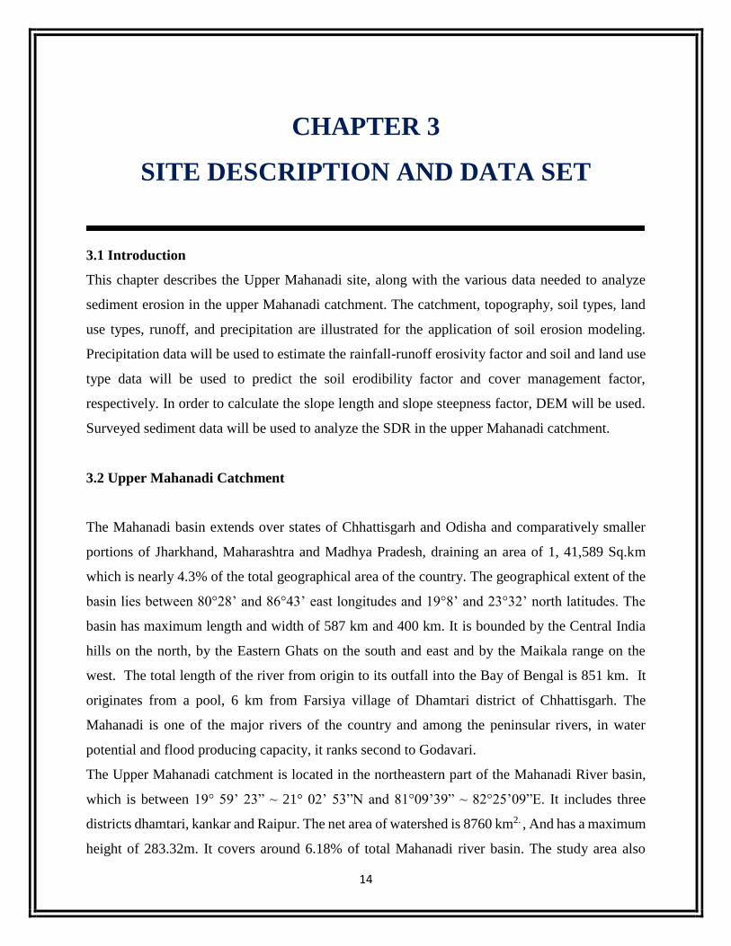
3.1 Introduction
This chapter describes the Upper Mahanadi site, along with the various data needed to analyze
sediment erosion in the upper Mahanadi catchment. The catchment, topography, soil types, land
use types, runoff, and precipitation are illustrated for the application of soil erosion modeling.
Precipitation data will be used to estimate the rainfall-runoff erosivity factor and soil and land use
type data will be used to predict the soil erodibility factor and cover management factor,
respectively. In order to calculate the slope length and slope steepness factor, DEM will be used.
Surveyed sediment data will be used to analyze the SDR in the upper Mahanadi catchment.
3.2 Upper Mahanadi Catchment
The Mahanadi basin extends over states of Chhattisgarh and Odisha and comparatively smaller
portions of Jharkhand, Maharashtra and Madhya Pradesh, draining an area of 1, 41,589 Sq.km
which is nearly 4.3% of the total geographical area of the country. The geographical extent of the
basin lies between 80°28’ and 86°43’ east longitudes and 19°8’ and 23°32’ north latitudes. The
basin has maximum length and width of 587 km and 400 km. It is bounded by the Central India
hills on the north, by the Eastern Ghats on the south and east and by the Maikala range on the
west. The total length of the river from origin to its outfall into the Bay of Bengal is 851 km. It
originates from a pool, 6 km from Farsiya village of Dhamtari district of Chhattisgarh. The
Mahanadi is one of the major rivers of the country and among the peninsular rivers, in water
potential and flood producing capacity, it ranks second to Godavari.
The Upper Mahanadi catchment is located in the northeastern part of the Mahanadi River basin,
which is between 19° 59’ 23” ~ 21° 02’ 53”N and 81°09’39” ~ 82°25’09”E. It includes three
districts dhamtari, kankar and Raipur. The net area of watershed is 8760 km2. , And has a maximum
height of 283.32m. It covers around 6.18% of total Mahanadi river basin. The study area also

15
includes three major dams such as Ravi Shankar dam and Dudhawa dam in Raipur. Murrum silli
dam near Kankar district.
Figure 3.1 sows the location of the upper Mahanadi river basin in Chhattisgarh, India. The main
gauging station (Raijm) is also located in the given map.
Figure 3.1 location of study area
Figure 3.1 represents the location of eight rainfall gauging station on Google map. Thiessen
polygon of the upper Mahanadi catchment is obtained by proximity tool of ArcGIS, and
coordinates was entered into the study area.

16
Figure 3.2 representing gauging station in upper Mahanadi catchment
3.3 Data Set of the Upper Mahanadi Catchment
Soil erosion is influenced by a variety of factors such as rainfall intensity and distribution, soil
types, topography of watershed, land use types, etc. These factors are presented very well with the
temporal and spatial type using GIS technique. GIS application is increasing more and more to
predict soil erosion in the watershed. In order to predict the soil erosion, sediment delivery ratio,
and trap efficiency in the upper Mahanadi catchment, the following spatial and temporal data are
used:
Digital Elevation Model (Data source: Catrosat v1.1, Bhuvan: 30 by 30m, year-2009)
2) Soil types map (Data source: F.A.O, vectorized map, year-2003)
3) Land cover type map (Data source: AWiFS, Bhuvan, cell size: 30mby 30m, 2009)
4) Daily precipitation data (Data source: India Meteorological Department)
6) Sediment Transportation survey report in the Upper Mahanadi catchment (Data source: India
Wris)

17
The India Wris has a database of suspended and runoff data from 1992 to 2010. It also has some
thematic maps, including a hydrologic units map, land cover map, soil type map, population
density map, etc. The precipitation data is available in Indian meteorological department from year
2004 to 2013 district wise on daily basis. This database is available at the web site;
http://www.India-wris.nrsc.gov.in
3.3.1 Digital Elevation Model
The DEM of the upper Mahanadi catchment is presented in Figure 3.3. This DEM was newly
created using the digital contour map (scale 1:5000). The watershed is delineated first for upper
Mahanadi catchment. The shape file is obtained from the raster image. Using that shape file the
DEM was extracted by mask extraction process. The terrain elevation of the upper Mahanadi
catchment ranges from EL.211m to EL.886m, with average elevation EL.426m. Using the DEM,
the following watershed and river characteristics can be predicted;
1) Watershed characteristics: drainage area, basin perimeter, effective basin width, form and shape
factor, drainage density, channel segment frequency, basin average elevation, basin slope, etc.
2) River characteristics: basin length, total stream length, channel slope, stream order, stream
length ratio, bifurcation ratio, etc.
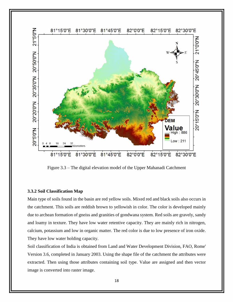
18
Figure 3.3 – The digital elevation model of the Upper Mahanadi Catchment
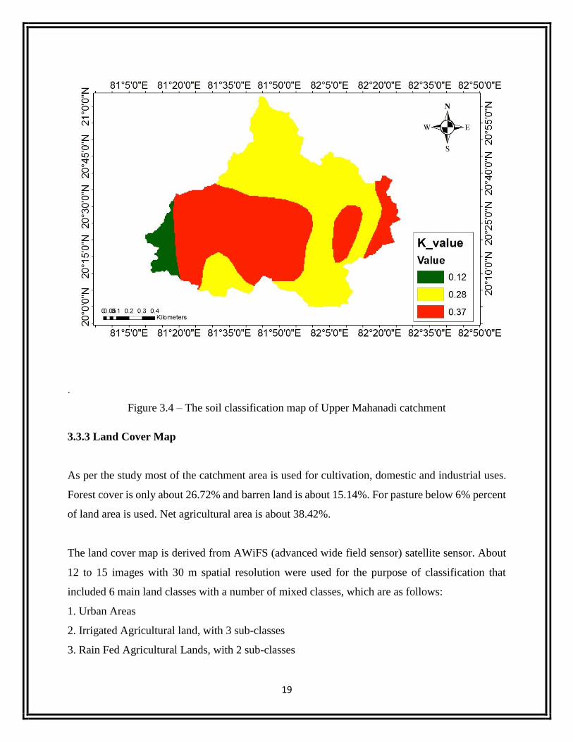
3.3.2 Soil Classification Map
Main type of soils found in the basin are red yellow soils. Mixed red and black soils also occurs in
the catchment. This soils are reddish brown to yellowish in color. The color is developed mainly
due to archean formation of gneiss and granities of gondwana system. Red soils are gravely, sandy
and loamy in texture. They have low water retentive capacity. They are mainly rich in nitrogen,
calcium, potassium and low in organic matter. The red color is due to low presence of iron oxide.
They have low water holding capacity.
Soil classification of India is obtained from Land and Water Development Division, FAO, Rome'
Version 3.6, completed in January 2003. Using the shape file of the catchment the attributes were
extracted. Then using those attributes containing soil type. Value are assigned and then vector
image is converted into raster image.
19
.
Figure 3.4 – The soil classification map of Upper Mahanadi catchment
3.3.3 Land Cover Map
As per the study most of the catchment area is used for cultivation, domestic and industrial uses.
Forest cover is only about 26.72% and barren land is about 15.14%. For pasture below 6% percent
of land area is used. Net agricultural area is about 38.42%.
The land cover map is derived from AWiFS (advanced wide field sensor) satellite sensor. About
12 to 15 images with 30 m spatial resolution were used for the purpose of classification that
included 6 main land classes with a number of mixed classes, which are as follows:
1. Urban Areas
2. Irrigated Agricultural land, with 3 sub-classes
3. Rain Fed Agricultural Lands, with 2 sub-classes

20
4. Natural Forests, with 2 sub-classes
5. Barren lands
6. Water Bodies
The developed map by AWiFS is used for the determination of this study. Figure 3.5 represents
land cover classification map of the upper Mahanadi catchment. Land cover assessment and
observing are essential for sustainability of natural resources.
Figure 3.5 shows the land classification of upper Mahanadi catchment derived by supervised
image classification. The areas having all the parameters are classified on the basis of color as
presented by NRS (national remote sensing institute)
3.5 Cover management factor of upper Mahanadi catchment

21
Table 3.2 presents station name, location, and beginning of observation of 8 rainfall gauging
stations in the upper Mahanadi catchment. All of them are managed by central water commission.
Daily rainfall and runoff records are available for 7 years of data from 2004 to 2014. Wischmeier
and Smith (1978) recommended that at least 20 years of rainfall data should be used to
accommodate natural climatic variation. Therefore, the upper Mahanadi catchment has a kind of
limitation to calculate the rainfall runoff erosivity factor of USLE.
Table 3.1 – Rainfall Gauging Stations
no Stations District Location
Latitude Longitude
Beginning of
observation
End of
observation
1 Charma Kankar 20.48450 81.373361 1.1.2004 30.12.2010
2 Gattasilli Raipur 20.450361 81.803306 1.1.2004 30.12.2010
3 Raijm Raipur 20.965 81.881667 1.1.2004 30.12.2010
4 Rudri Raipur 20.664481 81.552787 1.1.2004 30.12.2010
5 Kankar Kankar 20.270 81.490 1.1.2004 30.12.2010
6 Garibund Raipur 20.633 82.0667 1.1.2004 30.12.2010
7 Narharpur Kankar 20.4489 81.62036 1.1.2004 30.12.2010
8 Kurd Dhamtari 20.830 81.720 1.1.2004 30.12.2010

22
Figure 3.6 represent the thiessen polygon in upper Mahanadi catchment
Table 3.2 – Annual precipitation records
Station
Year
Charma Gattasilli Raijm Rudri Kankar Garibund Narharpur Kurd
2004 1037.8 939.2 9.932 939.2 1037.8 939.2 1037.8 916
2005 1245.7 1348 1348 1348 1245.7 1348 1245.7 1100.3
2006 1571.7 1206.7 1206.7 1206.7 1571.7 1206.7 1571.7 1320.4
2007 1235.7 1434.2 1434.2 1434.2 1235.7 1434.2 1235.7 1007.2

23
2008 652.2 1114.5 1114.5 1114.5 652.2 1114.5 652.2 901
2009 868.8 948.3 948.3 948.3 868.8 948.3 868.8 1113
2010 1480.8 1109.1 1109.1 1109.1 1480.8 1109.1 1480.8 1211.1
3.3.4 Discharge data
Average monthly flow data is collected from India-wris version 4.0 on upper Mahanadi Catchment
basin at Raijm gauging station. From the June to October (2004-2010 ).
Table 3.3 Represent the Discharge data
year Discharge data
cumec
2004 100.562
2005 88.2
2006 181.81
2007 141.17
2008 89.4485
2009 101.07
2010 111.9295
3.3.5 Sediment Survey Data
The most important study of sediment yield in the upper Mahanadi catchment was performed by
India-Wris. This study estimated sediment yields at proposed gauging station on the upper
Mahanadi catchment. The study was based on annually sediment yield estimated at the Raijm

24
gauging station. The observed sediment yield data is collected from India-wris during the period
2004 to 2010. The study did not exactly state how bed load amounts were accounted for the
sediment yield. Figure 3.3 shows location of the sediment gauge station along the basin and Table
3.3 presents sediment yield for the stations located in the upper Mahanadi catchment. The unit for
sediment yield for the river is given in ton of sediments per square kilometer of the catchment area
per year
Table 3.1 gives sediment yield in tons per year. This value is computed from suspended sediment
and discharge observed at the Raijm gauging station
Table 3.4 – Sediment Transportation data
Year Sediment Yield
in Tons/year
2004 3106.11
2005 3926.56
2006 4556.96
2007 6983.956
2008 5943.56

25
2009 5429.28
2010 6071.266
3.4 Summary
Chapter 3 demonstrates the upper Mahanadi catchment site description and data set: topography,
soil and land use characteristics, precipitation, runoff, and sediment survey data. Precipitation
and runoff data are needed to estimate the rainfall runoff erosivity factor (R). DEM, with 30m
grid cell size, is needed to analyze the slope length (L) and slope steepness (S). A soil map based
on vectorized feature data is used to estimate the soil erodibility (K) and transformed into the
raster data file with 30m grid cell size. A land cover map, extracted from AWiFS images, is used
to predict the cover management factor (C), which is one of the most sensitive factors in
analyzing the soil loss rates of the USLE model.

26
CHAPTER 4
METHODOLOGY AND PARAMETER
ESTIMATION
4.1 INTRODUCTION
This chapter describes the basic concepts, and the procedure for USLE model, in addition to the
methodology to estimate these six parameters, and prediction of the USLE model. Based on the
annual rainfall data, DEM, soil type map, and land cover map, six parameters of the USLE model
will be estimated and verified.
4.2 Watershed Delineation Process
It is a process of creating boundary of a watershed that represents the contributing area for
particular control point.
Step 1: cartosat image for required area is downloaded of 30m*30m resolution. Generally all the
files adjacent to upper Mahanadi river basin is downloaded.
Step 2: All the fill, flow direction and flow accumulation function was carried out by using
hydrology option of spatial analysis tool box.
Step 3: After carrying the above function, the pour point was selected. Pour point is a control point
for a particular watershed or a catchment. Coordinates of Raijm were selected and added to the
flow accumulation data.
Step 5: the pour point was snapped and using that snapped point and flow accumulation data a
watershed was generated.
Step 6: Similarly the above procedure unless a desired watershed was obtained.

27
4.3 USLE Parameter Estimation
The degree of erosion, specific degradation, and sediment yield from watersheds are related to a
complex interaction between topography, geology, climate, soil, vegetation, land use, and man-
made developments (Shen and Julien, 1993). The USLE is the method most widely used around
the world to predict long-term rates of inter rill and rill erosion from field or farm size units
subjected to different practices. Wischmeier and Smith (1965) developed the USLE based on many
years of data from about 10,000 small test plots throughout the U.S. Each test plot had about
22.13m flow lengths and they were all operated in a similar manner, allowing the soil loss
measurements to be combined into a predictive tool. Modified USLE (MUSLE) is an improvement
upon USLE (Williams, 1975) where by the soil loss from an isolated rainfall event can be
estimated. In MUSLE the rainfall energy term is replaced by a runoff energy factor. Sediment
yield for a rainfall event is given by: K, L, S, C, P factors remain the same as that for USLE.
The USLE model groups numerous physical and management parameters that influence erosion
under six factors, which can be expressed numerically. Interrelation between the variables
involved in erosion processes is represented in the flowchart shown in Figure 4.1.
Figure 4.1: Schematic Representation of USLE Components

28
Equation for Universal Soil Loss Equation is described below.
ARK L S C P (Eqn 4.1)
Where:
A = calculated average annual soil loss predicted and temporal average soil loss per unit of area.
A is expressed in unit tons/ (acre× yr.), but other units can be selected (that is, tons / (ha× yr.))
R= Rainfall-runoff erosivity factor (MJ mm ha -1 hr-1);
Erosivity factor is determined by both rainfall and the energy imparted to the land surface by the
rain drop effect.
K = Soil erodibility factor: It is defined as soil loss per unit of area for unit plot.
L = Slope length factor: It is the ratio of soil loss from field slope length to that from 22.13 m
length plot under identical conditions.
S = Slope steepness factor: It is the ratio of soil loss from the field slope gradient to that from 9 %
slope under otherwise identical conditions
C = Cover management factor : It is the expected ratio of soil loss from land cropped under
specified conditions to soil loss from clean, tilled fallow or identical soil and slope and under the
same rainfall.
P = Support practice factor: It is expressed as a ratio, which compares the soil loss from
investigated plot cultivated up and down the slope. P ranges from 1.0 for up and down cultivation
to 0.25 for contour strip cropping of gentle slope.
L and S factors are dimensionless parameters which represent the impact of topographic effects on
soil erosion rates. C and P factors stand for dimensionless impacts of cropping and management
systems on soil erosion control practices. L and S factors stand for the dimensionless impact of
slope length and steepness, and C and P represent the dimensionless impacts of cropping and
management systems and of erosion control practices. All dimensionless parameters are
normalized relative to the Unit Plot conditions, as described in Agriculture Handbook 703. Over
the years, the USLE and RUSLE became the standard tool for predicting soil erosion not only in
the U.S., but also throughout the world (Meyer, 1984). Widespread use has substantiated the
usefulness and validity of USLE for this purpose.

29
4.3.1 Rainfall-Runoff Erosivity Factor (R)
Wischmeier and Smith (1958) derived the rainfall and runoff erosivity factor from research data
from many sources. The rainfall – runoff erosivity factor is defined as the mean annual sum of
individual storm erosion index values, EI30, where E is the total storm kinetic energy and I30 is the
maximum rainfall intensity in 30 minutes. To compute storm EI30, continuous rainfall intensity
data are needed. Wishmeier and Smith (1978) recommended that at least 20 years of rainfall data
be used to accommodate natural climatic variation. Renard et al. (1997) states that the numerical
value used for R in USLE must quantify the effect of raindrop impact and must also reflect the
amount and rate of runoff likely to be associated with the rain. The rainfall runoff erosivity factor
(R) derived by Wischmeier appears to meet these requirements better than any of the many other
rainfall parameters and groups of parameters tested against the plot data. Wischmeier and Smith
(1965) found that the best predictor of rainfall erosivity factor (R) was:
Where:
R = rainfall-runoff erosivity factor—the rainfall erosion index plus a factor for any significant
runoff (100m×tonf×hect-1×yr-1)
E = the total storm kinetic energy in hundreds of m-tons per hect;
I30 = the maximum 30-minute rainfall intensity;
j= the counter for each year used to produce the average;
k= the counter for the number of storms in a year;
m= the number of storms n each year;
n= the number of years used to obtain the average R.
The calculated erosion potential for an individual storm is usually designated EI. The total annual
R is therefore the sum of the individual EI values for each rainfall storm event. The energy of a
rainfall storm is a function of the amount of rain and of all the storm’s intensity components. The
median raindrop size generally increases with greater rain intensity (Wischmeier et al., 1958), and
the terminal velocity of free-falling water drops increases with larger drop size (Gunn and Kinzer,

30
1949). To calculate the R-factor generally we used monthly, seasonal and annual rainfall data.
Rainfall erosivity estimation using rainfall data for different rain gauge station in Upper Mahanadi
catchment such as charma, gattasailli, Raijm, kankar, rudri, garibund, naraharpur, kurd.
Using the data for storms from several rain gauge stations located in different zones, linear
relationships were established between average annual rainfall and computed EI30 values for
different zones of India and iso-erodent maps were drawn for annual and seasonal EI30 values
(Ram Babu et al. 2004). Following equation was developed for upper Mahanadi river basin area
in Chhattisgarh India by Ram Babu et al. (2004) and used in the present study
R = 81.5 + 0.38RN (340 ≤ RN ≤ 3500 mm) …. (Eq. 2)
Where RN is the annual rainfall in mm. For the present study, Eq. 2 is used to compute annual
values of R-factor by replacing RN with actual observed annual rainfall in a year Figure 4.1 present
thiessen polygon maps of the Upper Mahanadi Catchment. The catchment boundaries and rain
gauge station are shown with the help of boundary lines and points.
Figure 4.2 showing thiessen polygon

31
In ARC GIS R factor is computed by putting the Coordinates of the gauging station for upper
Mahanadi catchment was obtained from Google. Then these longitude, latitude value are written
in excel and then imported into ARC GIS. These coordinates were super imposed on the shape file
of the upper Mahanadi catchment. Using Thiessen polygon command in proximity tool in analysis
tool box and excel latitude, longitude coordinates as input file, and thiessen polygon is drawn. In
the attribute of that polygon, gauging station name are entered corresponding to their coordinates.
Then weightage factor are derived, finally total rainfall values for each gauging station are inserted.
Then isoerodent value is computed for each field by using field calculator. Based on those
isoerodent value the polygon file was converted into raster image. Similarly these steps are
repeated for rainfall value of different year. A raster image of isoerodent value for upper Mahanadi
catchment for year 2009 is shown below.
Figure 4.3 showing R_factor variation
4.3.2 Soil Erodibility Factor (K)
Soil erodibility (K) represents the susceptibility of soil or surface material to erosion,
transportability of the sediment, and the amount and rate of runoff given a particular rainfall input,

32
as measured under a standard condition. The standard condition is the unit plot, 22.13m long with
a 9 percent gradient, maintained in continuous fallow, tilled up and down the hill slope (Weesies,
1998). K values reflect the rate of soil loss per rainfall-runoff erosivity (R) index. Soil erodibility
factors (K) are best obtained from direct measurements on natural runoff plots. Rainfall simulation
studies are less accurate, and predictive relationships are the least accurate (Romkens 1985). For
satisfactory direct measurement of soil erodibility, erosion from field plots needs to be studied for
periods generally well in excess of 5 years (Loch et al., 1998). Therefore, considerable attention
has been paid to estimating soil erodibility from soil attributes such as particle size distribution,
organic matter content and density of eroded soil (Wischmeier et al., 1971). Figure 4.4 represents
the nomograph used to determine the K factor for a soil, based on
its texture; % silt plus very fine sand, % sand, % organic matter, soil structure, and permeability.
Figure 4.4 – Soil erodibility nomograph (after Wischmeier and Smith, 1978).
33
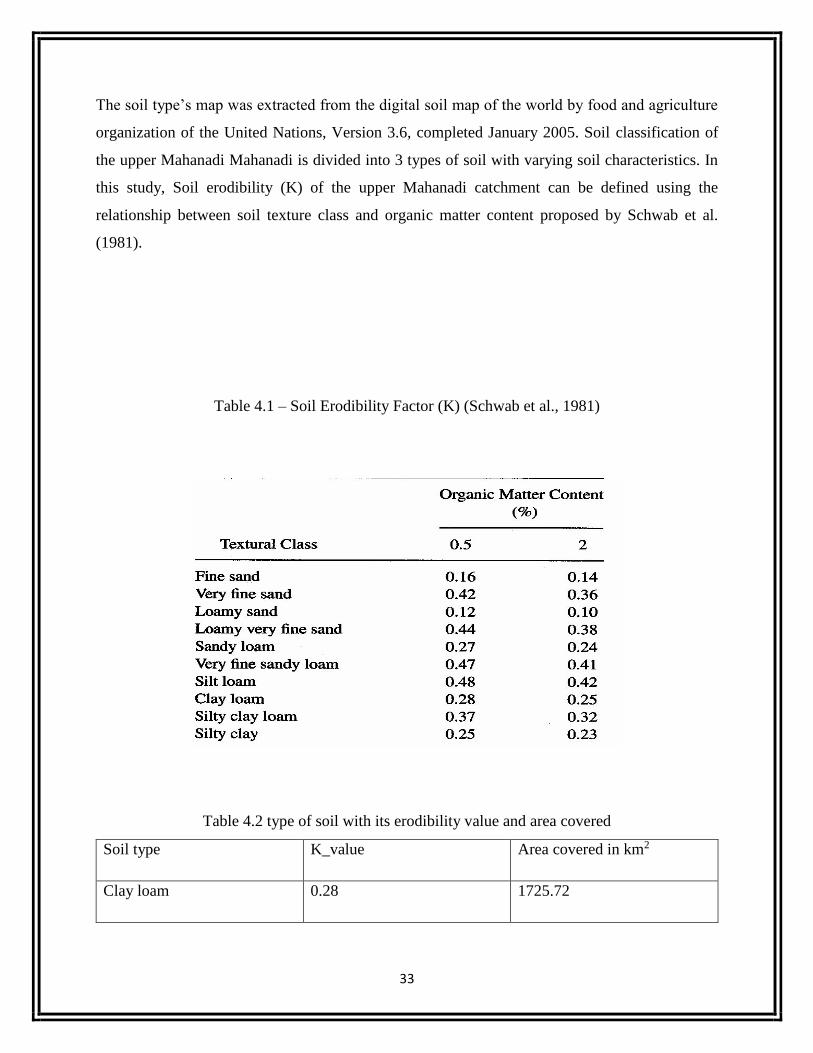
The soil type’s map was extracted from the digital soil map of the world by food and agriculture
organization of the United Nations, Version 3.6, completed January 2005. Soil classification of
the upper Mahanadi Mahanadi is divided into 3 types of soil with varying soil characteristics. In
this study, Soil erodibility (K) of the upper Mahanadi catchment can be defined using the
relationship between soil texture class and organic matter content proposed by Schwab et al.
(1981).
Table 4.1 – Soil Erodibility Factor (K) (Schwab et al., 1981)
Table 4.2 type of soil with its erodibility value and area covered
Soil type K_value Area covered in km2
Clay loam 0.28 1725.72

34
Silty clay loam 0.37 6464.88
Loamy sand 0.12 551.88
Figure 4.5 showing k map for upper Mahanadi catchment
4.3.3 Slope Length and Steepness Factor (LS)
The effect of topography on soil erosion is accounted for by the LS factor in
USLE, which combines the effects of a slope length factor, L, and a slope steepness factor, S. In
general, as slope length (L) increases, total soil erosion and soil erosion per unit area increase due
to the progressive accumulation of runoff in the downslope direction. As the slope steepness (S)
increases, the velocity and erosivity of runoff increase. The LS factor is computed by simple
formula as suggested by (Wischmeier and Smith, 1978) LSi = (Asi/22.13)n*(sinαi/0.0896)m.

35
Where Asi is the specific area at a shell I (=Aup/wn),
Aup: area of overland grid per unit width normal to direction of flow Wn.
αi= slope gradient in degrees for cell i. ,n=0.6 , m=1.3, gives consistent results in usle for slope length
<100m and angles <14 degrees.
Figure 4.6 – Schematic slope profiles of USLE applications (Renard et al., 1997)
LS Factor: This is Topological factor consisting of two sub-factors: slope gradient and slope
length factor; determined from DEM. These factors significantly influence soil erosion by surface
water movement. Slope length in meters (L) is calculated from the flow accumulation and slope
steepness in radian values. The LS factor is calculated using modification of the empirical equation
of Wischmeier and Smith, 1978 by Moore and Wilson (1992) using Spatial Analyst tool of ArcGIS
from equation 4:
[LS= power (“flow_accu”* cell size/22.1, 0.4) *power (sin (“slope_deg”*0.01745)/0.09, 1.4)*1.4]

36
Figure 4.7 slope map of upper Mahanadi in degree
Figure 4.8 shows flow accumulation of upper Mahanadi

37
Figure 4.9 LS factor computed for upper Mahanadi catchment
4.3.4 Cover Management Factor (C)
The cover management factor (C) represents the effects of vegetation, management, and erosion
control practices on soil loss. As with other USLE factors, the C value is a ratio comparing the
existing surface conditions at a site to the standard conditions of the unit plot as defined in earlier
chapters.
USLE uses a sub factor method to compute soil loss ratios (SLR), which are the ratios of soil loss
at any given time in the cover management sequence to soil loss from the standard condition. The
sub factors used to compute a soil loss ratio value are prior land use, forest cover, surface cover,
surface roughness, and soil moisture.
There are two C factor options in USLE, a time invariant option and a time variant option
(Kuenstler, 1998). In the case of Chhattisgarh, India, about two thirds of annual precipitation is
concentrated in the summer season, between July and September due to Monsoon effects. Due to
38
the precipitation pattern of India, a time invariant option is applied to the upper Mahanadi
catchment catchment.
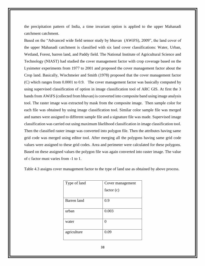
Based on the “Advanced wide field sensor study by bhuvan (AWiFS), 2009”, the land cover of
the upper Mahanadi catchment is classified with six land cover classifications: Water, Urban,
Wetland, Forest, barren land, and Paddy field. The National Institute of Agricultural Science and
Technology (NIAST) had studied the cover management factor with crop coverage based on the
Lysimeter experiments from 1977 to 2001 and proposed the cover management factor about the
Crop land. Basically, Wischmeier and Smith (1978) proposed that the cover management factor
(C) which ranges from 0.0001 to 0.9. The cover management factor was basically computed by
using supervised classification of option in image classification tool of ARC GIS. At first the 3
bands from AWiFS (collected from bhuvan) is converted into composite band using image analysis
tool. The raster image was extracted by mask from the composite image. Then sample color for
each file was obtained by using image classification tool. Similar color sample file was merged
and names were assigned to different sample file and a signature file was made. Supervised image
classification was carried out using maximum likelihood classification in image classification tool.
Then the classified raster image was converted into polygon file. Then the attributes having same
grid code was merged using editor tool. After merging all the polygons having same grid code
values were assigned to these grid codes. Area and perimeter were calculated for these polygons.
Based on these assigned values the polygon file was again converted into raster image. The value
of c factor must varies from -1 to 1.
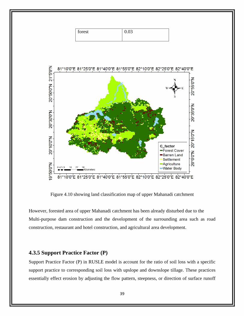
Table 4.3 assigns cover management factor to the type of land use as obtained by above process.
Type of land Cover management
factor (c)
Barren land 0.9
urban 0.003
water 0
agriculture 0.09
39
forest 0.03
Figure 4.10 showing land classification map of upper Mahanadi catchment
However, forested area of upper Mahanadi catchment has been already disturbed due to the
Multi-purpose dam construction and the development of the surrounding area such as road
construction, restaurant and hotel construction, and agricultural area development.
4.3.5 Support Practice Factor (P)
Support Practice Factor (P) in RUSLE model is account for the ratio of soil loss with a specific
support practice to corresponding soil loss with upslope and downslope tillage. These practices
essentially effect erosion by adjusting the flow pattern, steepness, or direction of surface runoff
40
and by reducing the amount and rate of runoff (Reynard and Foster 1983). The support practices
for cultivable lands are including contouring, strip-cropping, terracing, and subsurface drainage.
While on dry land or rangeland area, soil disturbing practices to result storage of moisture and
reduction of runoff considered to be as support practices mechanisms.
Support Practice Factor (P) is ranged from 0 to 1. It is equal to 1 when the land is directly plowed
on the slope and less than 1 when the adopted conservation practice reduces soil erosion. Terracing
and contouring are common and effective support practices on the field level. The effects of
terracing are reflected in the hill slope length and gradient, because it reduces the length of the hill
slope. Contouring changes the flow direction and cause runoff to flow around the hill slope rather
than directly downslope.
Currently there are no support practices in place within the study site. The common practice is to
assign a value of 1 for the P factor. For future use, after calculating the estimated soil loss by
USLE, the P factor values can be adjusted to forecast various prevention measures.
4.4 Summary
Chapter 4 presents the procedure and methodology of the USLE parameter estimation. USLE has
six parameters, which are rainfall erosivity (R), soil erodibility (K), slope length and steepness
(LS), cover management (C), and support practice factor (P). In the upper Mahanadi catchment,
the annual average R values range from 164 to 504.44 based on the location of rainfall stations.
Kurd, Dhamitri located in the southeastern part of the watershed presents the maximum R value
of 504.44. Based on the soil classification and organic matter, soil erodibility (K) is estimated and
varies from 0.13 to 0.38. Slope length and steepness (LS) is predicted using the DEM and Arc info
AML developed by Van Remortel et al. (2001). LS values range from 0 to 44. The cover
management factor (C) is calculated from AWiFS data obtained from bhuvan. Forested area C
value is estimated using a “Trial and Error method” from the relationship between the annual soil
losses and various sediment delivery ratio models. As most of the land area is covered by forest
and agriculture the cover management factor varies from 0.003 to 0.9. Since no support practice
factor is like strip cropping, contour cropping is practiced in that area so support practice factor is
taken as 1.

41
Chapter 5
RESULTS AND DISCUSSION
5.1 Introduction
This chapter deals with the application and results of the USLE model; the annual average soil loss
rate, upper Mahanadi catchment. The results of these cases will be analyzed and compared based
on the spatial and temporal variation. Based on the land cover in upper Mahanadi, the spatial
distribution pattern of soil loss rate will be analyzed. The basic concept of the Sediment Delivery
Ratio (SDR) will be described and total soil loss rate in the upper Mahanadi catchments are
analyzed.
5.2 Events Simulation of Soil Loss Rate
In order to simulate upland erosion at upper Mahanadi catchment, three cases will be modeled. In
performing this analysis, each thematic map, which is the same grid cell size and coordination,
will be used. The rainfall runoff erosivity factor (R) varies spatially and temporally throughout the
upper Mahanadi catchment. In contrast, the soil erosivity factor (K), the slope length and steepness
factor (LS), the cover management factor (C), and support practice factor (P) are considered to be
constant throughout the upper Mahanadi catchment. Computed annual average soil loss rate will
be used to estimate the SDR at the upper Mahanadi catchment as representing the relationship
between annual average soil loss rate and surveyed sediment deposits.
5.3 The Annual Average Soil Loss Rate
The occurrence of soil erosion has a close relationship with the status of land use and the situation
of farmland management along with topographical characteristics such as slope length and
steepness. As mentioned previously in chapter 4.3.4, the cover management factor of forested area
is calculated by the method of supervised classification in ARC GIS.

42
Table 5.1 presents the results of the annual soil loss rate and SDR estimated according to the
variable C values of forested area. Figure 5.1 represents the relationship graph between the annual
average soil loss rate and SDR including the observed sediment deposits and SDR values estimated
using the basin characteristics. Based on the SDR values estimated by Renfro (1975), Williams
(1977), and Roehl (1962), and surrounding development situations of the upper Mahanadi
catchment, the appropriate C value range for forested area can be chosen as 0.03 in this study.
5.3.1 Computed pixel wise sediment yield for year 2004
Following are 5 parameters used for calculating sediment yield.
1) Rainfall runoff erosivity factor (R): 418.72 ~ 475.84 MJ mm ha-1 hr-1
2) Soil erodibility factor (K): 0.12 ~ 0.37
3) Slope length factor & slope steepness factor (LS): 0 ~ 43.99
4) Cover management factor (C): 0 ~ 1
5) Support practice factor (P): 1
Figure 5.3.1.a shows multiplication of all four parameters of USLE. The images are multiplied
pixel by pixel in raster calculator in arc map function of spatial analysis tool box. The maximum
value obtained is 33.1033 per hector per year.
Figure 5.3.1.a Annual Average Soil loss rate map of the upper Mahanadi
catchment in year 2004

43
5.3.1.b the figure below represents the product of all four factors of USLE. After adding all the
unique values of the pixel, the net sediment yield in tons per year is 4297.36. Observed sediment
yield at the gauging station computed from daily data of discharge and suspended sediment
obtained from India Wiris is 3106.11 in tons per year. The error obtained is 22.4%
Figure 5.3.1.b sediment yield in tons per hect per year 2004
Table 5.3.1.a the coordinates obtained for highest soil erosion for a particular area is shown in
table below. These coordinates are obtained by using identification tools of ARC GIS on the annual
average soil loss rate map.

44
Table 5.3.1.a shows the maximum erosion prone area in the catchment area in
the year 2004 (source field study)
LATITUDE LONGITUDE PLACE OF
SEDIMENT
EROSION
STATE
20.485658 81.396527 Nawagaon Saradui Chhattisgarh
20.519208 81.381536 Charama, Kanker Chhattisgarh
20.691957 81.652081 Dhamtari Chhattisgarh
20.684818 81.641374 Dhamtari Chhattisgarh
20.429264 82.678243 Lambipani Chhattisgarh
5.3.2 Computed pixel wise sediment yield for year 2005
Following are 5 parameters used for calculating sediment yield.
1) Rainfall runoff erosivity factor (R): 480.94 ~ 593.74 MJ mm ha-1 hr-1
2) Soil erodibility factor (K): 0.12 ~ 0.37
3) Slope length factor & slope steepness factor (LS): 0 ~ 43.99
4) Cover management factor (C): 0 ~ 1
5) Support practice factor (P): 1
Figure 5.3.2.a shows multiplication of all four parameters of USLE. The images are multiplied
pixel by pixel in raster calculator in arc map function of spatial analysis tool box. The maximum
value obtained is 24.132 per hector per year.

45
Figure 5.3.2.a Annual Average Soil loss rate map of the upper Mahanadi catchment in year 2005
5.3.2.b The below figure is product of all four parameters on pixel basis . The highest value of
theoretical sediment yield in tons per hector per year is 33.1033. After adding all the pixel values
the net sediment yield in tons per year is 5065.26 Observed sediment yield at the gauging station
computed from daily data of discharge and suspended sediment obtained from India Wiris is
3926.56 in tons per year. The error obtained is 29.7%.

46
Figure 5.3.2.b sediment yield in tons per hect per year 2005
Table 5.3.2.a the coordinates obtained for highest soil erosion for a particular area is shown in
table below. These coordinates are obtained by using identification tools of ARC GIS on the annual
average soil loss rate map.
Table 5.3.2.a shows the maximum erosion prone area in the catchment area in
the year 2005 (source field study)
LATITUDE LONGITUDE PLACE OF
SEDIMENT EROSION
STATE
20.536340 82.213158 Chikhli Chhattisgarh
20.427837 82.077529 Gariaband Chhattisgarh
20.311841 81.901211 Bhiterras Chhattisgarh

47
20.266133 81.628881 Saranda Chhattisgarh
20.486728 81.397598 Nawagaon Saradui Chhattisgarh
5.3.3 Computed pixel wise sediment yield for year 2006
Following are 5 parameters used for calculating sediment yield.
1) Rainfall runoff erosivity factor (R): 540.046 ~ 678.746 MJ mm ha-1 hr-1
2) Soil erodibility factor (K): 0.12 ~ 0.37
3) Slope length factor & slope steepness factor (LS): 0 ~ 43.99
4) Cover management factor (C): 0 ~ 1
5) Support practice factor (P): 1
Figure 5.3.3.a shows multiplication of all four parameters of USLE. The images are multiplied
pixel by pixel in raster calculator in arc map function of spatial analysis tool box. The maximum
value obtained is 28.1768 per hector per year.
Figure 5.3.3.a Annual Average Soil loss rate map of the upper Mahanadi catchment in year 2006

48
5.3.3.b The below figure is product of all four parameters on pixel basis . The highest value of
theoretical sediment yield in tons per hector per year is 28.176. After adding all the pixel values
the net sediment yield in tons per year is 5650.33 Observed sediment yield at the gauging station
computed from daily data of discharge and suspended sediment obtained from India Wiris is
4556.986 in tons per year. The error obtained is 24.22%.
Figure 5.3.3.b sediment yield in tons per hect per year 2006
Table 5.3.3.a the coordinates obtained for highest soil erosion for a particular area is shown in
table below. These coordinates are obtained by using identification tools of ARC GIS on the annual
average soil loss rate map.
Table 5.3.3.a shows the maximum erosion prone area in the catchment area in
the year 2006 (source field study)
LATITUDE LONGITUDE PLACE OF SEDIMENT
EROSION
STATE
20.489584 81.393315 Kanker Chhattisgarh

49
20.503860 81.574630 Kariyapahad Chhattisgarh
20.685175 81.641017 Dhamtari Chhattisgarh
20.426766 82.077172 Gariaband Chhattisgarh
20.872915 81.820190 Charbhatha Chhattisgarh
5.3.4 Computed pixel wise sediment yield for year 2007
Following are 5 parameters used for calculating sediment yield.
1) Rainfall runoff erosivity factor (R): 464.236 ~ 626.572 MJ mm ha-1 hr-1
2) Soil erodibility factor (K): 0.12 ~ 0.37
3) Slope length factor & slope steepness factor (LS): 0 ~ 43.99
4) Cover management factor (C): 0 ~ 1
5) Support practice factor (P): 1
Figure 5.3.4.a shows multiplication of all four parameters of USLE. The images are multiplied
pixel by pixel in raster calculator in arc map function of spatial analysis tool box. The maximum
value obtained is 47.3125 per hector per year.
Figure 5.3.4.a Annual Average Soil loss rate map of the upper Mahanadi catchment in year 2007

50
5.3.4.b The below figure is product of all four parameters on pixel basis . The highest value of
theoretical sediment yield in tons per hector per year is 47.312. After adding all the pixel values
the net sediment yield in tons per year is 8969.89. Observed sediment yield at the gauging station
computed from daily data of discharge and suspended sediment obtained from India Wiris is
6983.95 in tons per year. The error obtained is 22.14%.
Figure 5.3.4.b sediment yield in tons per hect per year 2007
Table 5.3.4.a is a tabular representation of the coordinates obtained by estimation for highest
erosion in the year 2007. These coordinates are obtained by using identification tools of ARC GIS
on the annual average soil loss rate map. Then these coordinates were used in lat long.net website
to find out name and district of the area.

51
Table 5.3.4.a shows the maximum erosion prone area in the catchment area in
the year 2007 (source field study)
LATITUDE LONGITUDE PLACE OF
SEDIMENT
EROSION
STATE
20.692314 81.653866 Dhamtari Chhattisgarh
20.720867 81.722394 Donar Chhattisgarh
20.868632 81.896571 Kuruskera Chhattisgarh
20.296133 81.628881 Deoribalaji Chhattisgarh
20.520993 81.379752 Bhelai Chhattisgarh
5.3.5 Computed pixel wise sediment yield for year 2008
Following are 5 parameters used for calculating sediment yield.
1) Rainfall runoff erosivity factor (R): 329.336 ~ 505.01 MJ mm ha-1 hr-1
2) Soil erodibility factor (K): 0.12 ~ 0.37
3) Slope length factor & slope steepness factor (LS): 0 ~ 43.99
4) Cover management factor (C): 0 ~ 1
5) Support practice factor (P): 1
Figure 5.3.5.a shows multiplication of all four parameters of USLE. The images are multiplied
pixel by pixel in raster calculator in arc map function of spatial analysis tool box. The maximum
value obtained is 38.133 per hector per year.

52
Figure 5.3.5.a Annual Average Soil loss rate map of the upper Mahanadi catchment in year 2008
5.3.5.b The below figure is product of all four parameters on pixel basis . The highest value of
theoretical sediment yield in tons per hector per year is 38.133. After adding all the pixel values
the net sediment yield in tons per year is 6495.97. Observed sediment yield at the gauging station
computed from daily data of discharge and suspended sediment obtained from India Wris is

53
5943.56 in tons per year. The error obtained is 8.5%.
Figure 5.3.5.b sediment yield in tons per hect per year 2008
Table 5.3.5.a the coordinates obtained for highest soil erosion for a particular area is shown in
table below. These coordinates are obtained by using identification tools of ARC GIS on the annual
average soil loss rate map.
Table 5.3.5.a shows the maximum erosion prone area in the catchment area in the
year 2008 (source field study)
LATITUDE LONGITUDE PLACE OF
SEDIMENT EROSION
STATE
20.485301 81.397598 Nawagaon Saradui Chhattisgarh
20.426766 82.077172 Gariaband Chhattisgarh
20.867918 81.896571 Kuruskera Chhattisgarh

54
20.78701 81.787354 Dhamtari Chhattisgarh
20.691600 81.653866 Dhamtari Chhattisgarh
5.3.6 Computed pixel wise sediment yield for year 2009
Following are 5 parameters used for calculating sediment yield.
1) Rainfall runoff erosivity factor (R): 411.56 ~ 504.44 MJ mm ha-1 hr-1
2) Soil erodibility factor (K): 0.12 ~ 0.37
3) Slope length factor & slope steepness factor (LS): 0 ~ 43.99
4) Cover management factor (C): 0 ~ 1
5) Support practice factor (P): 1
Figure 5.3.6.a shows multiplication of all four parameters of USLE. The images are multiplied
pixel by pixel in raster calculator in arc map function of spatial analysis tool box. The maximum
value obtained is 33.36 per hector per year.
Figure 5.3.6.a Annual Average Soil loss rate map of the upper Mahanadi catchment in year 2009
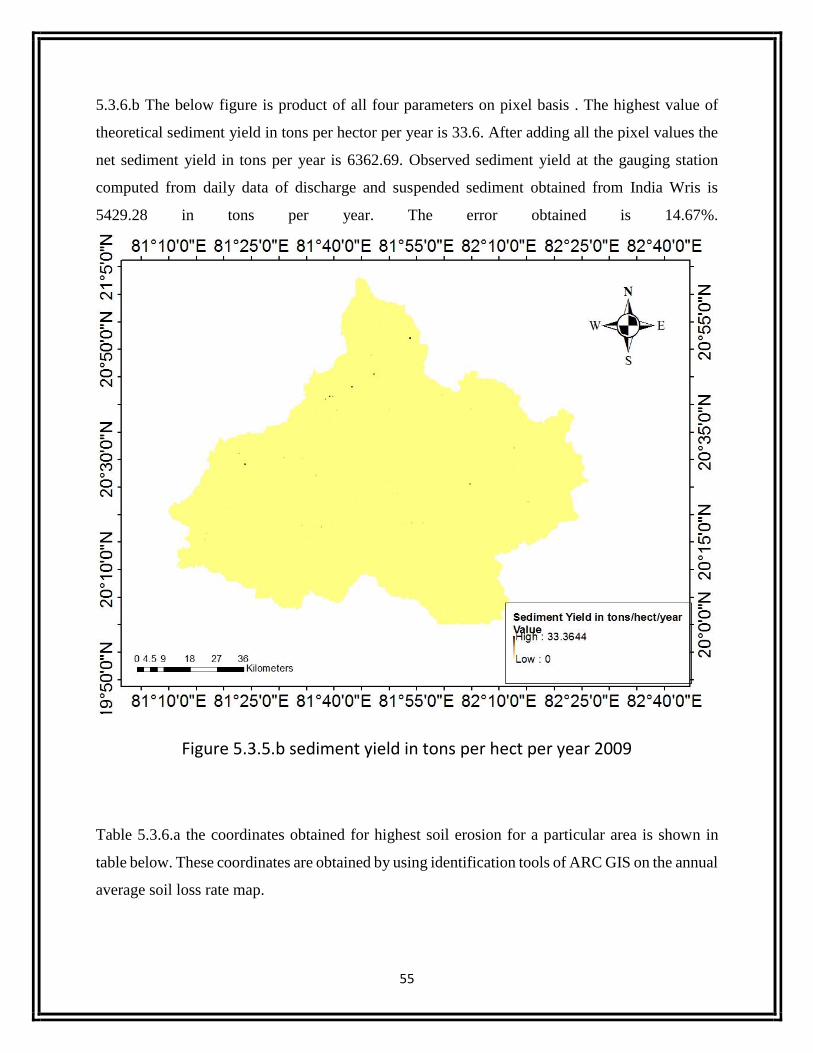
55
5.3.6.b The below figure is product of all four parameters on pixel basis . The highest value of
theoretical sediment yield in tons per hector per year is 33.6. After adding all the pixel values the
net sediment yield in tons per year is 6362.69. Observed sediment yield at the gauging station
computed from daily data of discharge and suspended sediment obtained from India Wris is
5429.28 in tons per year. The error obtained is 14.67%.
Figure 5.3.5.b sediment yield in tons per hect per year 2009
Table 5.3.6.a the coordinates obtained for highest soil erosion for a particular area is shown in
table below. These coordinates are obtained by using identification tools of ARC GIS on the annual
average soil loss rate map.

56
Table 5.3.6.a shows the maximum erosion prone area in the catchment area in
the year 2009 (source field study)
LATITUDE LONGITUDE PLACE OF
SEDIMENT EROSION
STATE
20.867918 81.897304 Kuruskera Chhattisgarh
20.485746 81.397897 Nawagaon Saradui Chhattisgarh
20.519535 81.380289 Kanker Chhattisgarh
20.426974 82.078066 Gariaband Chhattisgarh
20.535834 82.212268 Chikhli Chhattisgarh
5.3.7 Computed pixel wise sediment yield for year 2010
Following are 5 parameters used for calculating sediment yield.
1) Rainfall runoff erosivity factor (R): 502.95 ~ 644.204 MJ mm ha-1 hr-1
2) Soil erodibility factor (K): 0.12 ~ 0.37
3) Slope length factor & slope steepness factor (LS): 0 ~ 43.99
4) Cover management factor (C): 0 ~ 1
5) Support practice factor (P): 1
Figure 5.3.7.a shows multiplication of all four parameters of USLE. The images are multiplied
pixel by pixel in raster calculator in arc map function of spatial analysis tool box. The maximum
value obtained is 37.97 per hector per year.

57
Figure 5.3.7.a Annual Average Soil loss rate map of the upper Mahanadi catchment in year 2010
5.3.7.b The below figure is product of all four parameters on pixel basis . The highest value of
theoretical sediment yield in tons per hector per year is 37.97. After adding all the pixel values
the net sediment yield in tons per year is 7218.09. Observed sediment yield at the gauging station
computed from daily data of discharge and suspended sediment obtained from India Wris is
6071.26 in tons per year. The error obtained is 18.88%.
Figure 5.3.7.b sediment yield in tons per hect per year 2010

58
Table 5.3.6.a the coordinates obtained for highest soil erosion for a particular area is shown in
table below. These coordinates are obtained by using identification tools of ARC GIS on the annual
average soil loss rate map.
Table 5.3.7.a shows the maximum erosion prone area in the catchment area in the
year 2010 (source field study)
LATITUDE LONGITUDE PLACE OF SEDIMENT
EROSION
STATE
20.683717 81.640483 Dhamtari Chhattisgarh
20.691332 81.655712 Rudari Chhattisgarh
20.758432 81.789437 Kareli Chhoti Chhattisgarh
20.868364 81.896037 Kuruskera Chhattisgarh
20.426974 82.078066 Gariabanda Chhattisgarh
5.4 Tabular representation of observed, computed sediment yield and
sediment delivery ratio.
This table 5.4 represents gauging station wise observed and computed sediment yield. The
sediment delivery ratio for the catchment area is also shown in the table. The sediment delivery
ratio is the gross sediment yield at the outlet point of the gauging station. It is obtained by
dividing the observed sediment by area of the basin.

59
Table: 5.4 Comparison between observed and computed values of sediment yield
(source field study)
Year Gauging
station
Sediment
delivery
ratio
Observed
sediment yield
in tons/year
Computed
sediment yield
in tons/year
Percentage of
error
2004 Raijm 0.35 3106.11 4297.36 22.4
2005 Raijm 0.448 3926.56 5065.26 29.7
2006 Raijm 0.52 4556.96 5650.63 24.22
2007 Raijm 0.43 6983.956 8969.89 22.14
2008 Raijm 0.304 5943.56 6495.97 8.5
2009 Raijm 0.44 5429.28 6362.69 14.67
2010 Raijm 0.69 6071.266 7218.09 18.88

60
CHAPTER 06
SUMMARY AND CONCLUSIONS
6.1 Summary and Conclusions
The fluvial system consisting of upland erosion zone, transportation zone and downstream sediment
zone is an open system that is susceptible to modification by climate change and human activities.
Changes of erosion pattern of upstream of Mahanadi river basin affect the sedimentation rate of
downstream river basin. If a relationship between factors affecting the soil erosion can be established,
then future scenarios can be predicted in response to global climate change and urban expansion. The
present study has been formulated to understand these factors affecting the sedimentation of Mahanadi
river basin. The discharge and suspended data collected from India Wris have been analyzed to study
sediment carrying capacity of Mahanadi River Basin on annual basis.
6.2 Specific conclusions related to Upper Mahanadi catchment are
1. The annual average soil loss rate of the Upper Mahanadi catchment were estimated to be 8969.89
tons/hect/year of 2006 to 2010
2. In case of the spatial distribution of erosion rates at the Upper Mahanadi Catchment, the relationship
between probability and annual average soil loss rates is analyzed. The analysis indicated that up to
seventy percent of the mean annual soil loss rates are in the range of tolerable soil loss rate (0 – 5
tons/acre/year). Moreover, south western part of the basin is prone to extensive erosion than the eastern
part.
3. Sediment yield of all seven years are compared and maximum erosion obtained is below 30%.
Erosion prone areas are located in the catchment.
4. Type of soil found out is laterite soil, kankar and red yellow soil. Slope stiffness factor obtained is
less than 40. Results obtained from the present study work are very good. Therefore, more study should
be done to find out actual location of erosion prone areas and to follow different types of cultivation
or forestation in order to prevent soil erosion

61
FUTURE SCOPE OF STUDY
• This study helps to calculate the change of cross section of the river basin due to sediment
deposited.
• This study will help us to use better sediment prediction models like MUSLE and RUSLE to
calculate more precise sediment yield.
• This study helps to predict suspended load concentration at the gauging site.
• This study helps to perform various hydrological operations like flood routing, determination of
capacity and water spread corresponding to each elevation.
• This study helps in identifying the erosion prone areas of the river basin.
• This helps for taking measures for conservation of soil that can be implemented on those areas
for checking of siltation of soil.

62
CHAPTER 8
REFERENCE
Narayan, D. and Babu, R. (1983) ‘estimation of soil erosion in India’ American society
of civil engineering 0733-9437.
Subramanian, V. (1996) ‘The sediment load of Indian rivers, erosion and sediment
yield’, Global and regional perspective IAHS publication number 236.
Wayne, D.E. and Saynor, M.J. (1996) ‘success of soil conservation work in reducing soil
erosion rate and sediment yield in central eastern Australia’, global and regional
perspectives IAHS publication number 236
Kothyari, U, (1996) ‘Erosion and sedimentation’, Erosion and Sedimentation, Global and
Regional perspective IAHS publication number 236.
Jinze, M. (1996) ‘ Recent studies of the role of soil conservation in reducing erosion
and sediment yield in the loess plateau of yellow river basin’, Erosion and sediment
yield IAHS publication number 236.
Adinarayan, J. (1996) ‘Prioritization of basins on a silt index –an integrated graph
approach’, Eosion and sediment yield IAHS publication number 236.
Kothyar, U.C and Jain, S.K. (1997) ‘sediment yield estimation using GIS’, Hydrological
since journal 42(6).
Jain, S.K., Kumar, S. and Varghese, J. (2001) ‘Estimation of soil erosion of Himalayan
watershed using GIS technique’, water resource management vol-15.
Singh, V.P. and Woolhiser, (2002) D.A. ‘Mathematical modelling of watershed
hydrology’, American Society of Civil Engineering 10.1061.
Erskine, D.W. , Mahamudzdeh, A. and Myers, C. (2002) ‘land use effects of sediment
yield and soil erosion rates in small basin of Trassic sandstone near Sydney ,
Australia’, Elsevier catena 49
Ahmad, I. and Verma, M.K. (2003) ‘Application of USLE model And GIS in estimation
of soil erosion of tandula reservoir’, International Journal of emerging Technology and
advance engineering volume-3, issue 4.
Bhattari, R. and Dutta, D. (2006) ‘ Estimation of soil erosion and sediment yield using
GIS at catchment scale’ , By springer since
Raghuswanshi, N.S., Singh.R and Reddy L.S. (2006) ‘Run off and sediment yield
modelling using artificial neural network upper sewane river india’, American society
of civil engineering 1084-1699.
Pandey, A., Chowdary, V.M, and Mal, B.C, (2006) ‘Identification of Critical erosion
prone areas in small agricultural watershed using USLE and remote sensing’,
Springer since and business media.

63
Jackson, W.L. and Gebharlt, K. (2007) ‘Use of modified Universal Soil Loss Equation
for average small sediment yield estimate of small range land drainage basin’,
Hydrologist USDI Bureau Of land Management.
Kate, C. and Sumi, T. (2008) ‘Sedimentation yield and transportation analysis case
study of managawa river basin’, Annual Hydraulic Engineering, JSCE volume.52.
Dubral, P.P., Baithuri, N. and Pandey, A. (2008) ‘soil erosion assessment in hilly
catchment of eastern India using USLE and remote sensing’, Water Resource Manage
, springer since -008-92539.
Carolina B.F., Joris, D.V. and Castillo, V. (2008) ‘The impact of land use change and
check dams on catchment sediment yield’, hydrologic process wiley inter since.
Jain, M.K. and Das, D. (2009) ‘Estimation of sediment yield areas of soil erosion and
deposition of watershed prioritization using GIS and remote sensing’, Water resource
Mange Springer Since.
Arekhi, S. and Shabani, A. (2010) ‘Applcation of modified universal soil loss equation
in prediction of sediment yield case study: kengir watershed Iran’, Saudi Society of
Geo since.
Arekhi, S. and Rostamizad, G. (2011) ‘Sediment yield estimating from three micro-
watersheds by integrated KWGIUH and MUSLE models’, Elixir Agriculture (36)
3190-3199.
Cornia, A. and Viorel, A. (2011) ‘The quantitate estimation of the soil erosion using
USLE type Romsen model’, Carpathian journal of earth and environmental since, vol-6,
page 59-66.
Parveen, R. and Kumar, U. (2012) ‘ Integrated approach of universal soil loss equation
and geographic information system for soil loss risk assessment in upper south koel
basin’, journal by geographic information system, published by scientific research vol-4 .