APPLICATION OF THE OPTION MARKET

A P P L I C A T I O N OF T H E O P T I O N M A R K E T

P A R A D I G M TO T H E S O L U T I O N OF I N S U R A N C E P R O B L E M S

- - D I S C U S S I O N - -

STEPHEN MILDENHALL

1. INTRODUCTION

Mr. Wacek's paper is based on the well known fact that the Black-Scholes call

option price is the discounted expected excess value of a certain lognormal random

variable.1 Specifically, the Black-Scholes price can be written as

B S = e - " ( T - t ) E [ ( ~ ' ( T ) - k) +]

where r is the risk free rate of interest, T is the time when the option expires, t is the

current time, S(T) is a lognormal random variable related to the stock price S ( T )

at time T, k is the exercise price, and x + := max(x, 0). In insurance terms, ( L - k) +

represents the indemnity payment on a policy with a loss of L and a deductible k.

The Black-Scholes price can also be regarded as the discounted insurance charge,

see Gillam and Snader [18] or Lee [25]. It is easy to compute the insurance charge

1 The formula is explicit in virtually all financial economics derivations, for ex-

ample, Merton [27] page 283, Cox and Ross [4] page 154 equation 19 which is

essentially the author 's Equation (1.3), Harrison and Kreps [19] Corollary to Theo-

rem 3, Karatzas and Shreve [23] page 378, Hull [20] page 223 (for forward contracts

on a stock), as well as more overtly actuarial works, such as Gerber and Shiu [17]

page 104, and Kellison [24] Appendix X. \

Typcset by ,A.h&.~-TEX 1

2 STEPHEN MiLDENHALL

under the lognormal assumption to arrive a t - -bu t not to derive - the explicit Black-

Scholes formula. 2

Even without reference to the Black-Scholes formula there are obvious analogies

between insurance and options because both are derivatives. An insurance payment

is a function of--is derived f rom-- the insured's actual loss; similarly the terminal

value of an option is a function of the value of some underlying security. To the

extent that options and insurance use the same functions to derive value there will

be a dictionary between the two. As Mr. Wacek points out, this is the case. For

example, the excess function (L - k) + is used to derive the terminal value of a call

and an insurance payment with a deductible k; min(L, l) determines the value of an

insurance contract with a limit l; and (k - L) + = k - min(L, k) gives the terminal

value of a put option as well as the insurance savings function. There are several

other examples given in the paper, including a cylinder. The author explains how an

insurance cylinder can be used to provide cheaper reinsurance and greater earnings

stability for the cedent. The idea of regarding an insurance payment as a function

of the underlying loss has been discussed previously in the Proceedings by Lee [25],

[26], and Miccolis [28]. The connection between insurance and options, based on

the fact that both are derivatives, was also noted in D'Arcy and Doherty [9] page

57.

Here are two other interesting correspondences between option structures and

insurance. The first is the translation from put-call parity in options pricing to

the relationship "one plus savings equals entry ratio plus insurance charge" from

retrospective rating. The put option is equivalent to the insurance savings function

and the call option to the insurance charge function. See Lee [25] and [26], which

has the options profit diagrams, or Gillam and Snader [18] for more details.

The second correspondence applies Asian options to a model of the rate of claims

payment or reporting in order to price catastrophe index futures and options. This

example is too involved to describe in detail here; the interested reader should look

in the original papers by Cummins and Geman, [7] and [8].

2 Kellison [24] Appendix X gives all the details.

APPLICATION OF THE OPTION MARKET PARADIGM 3

[nsurance can also be regarded as a swap transaction. Hull [20] defines swaps

generically as "private agreements between two cornpanies to exchange cash flows in

tile future according to a prearranged formula." In insurance language one cash flow

is the known premium payment, generally consisting of one or more installments

during the policy period, and the other varies according to losses and continues for

a longer period of time. Many recent securitized transactions have been st~:uctured

as swaps. Indeed, in that context a swap is essentially insurance from a non-

insurance company counter-party. I regard swaps as a better model for insurance

than options because they involve a series of cash flows into the future rather than a

single payment. With options there is a single payment when the option is exercised.

Clearly this is not such a good model for a per occurrence insurance product that

could cover many individual claims.

Despite the title of the paper, Mr. Wacek is more concerned with options not-

at ion-puts , calls, profit diagrams and so fo r th - - than with the options market

paT"adigrn. A paradigm is a "philosophical and theoretical framework of a scientific

school or discipline within which theories, laws, and generalizations. . , are formu-

lated" (Merriam Webster's). Mr. Wacek's paper does not discuss the assumptions

underlying Black-Scholes nor the derivation of the formula in any detail. Both are

an important part of the options pricing paradigm. Moreover, the comments he

offers on options prices tend to confuse a pure premium (loss c o s t ) w i t h a price

(loss cost including risk charge, in this context). He rightly draws a distinction

between the two but does not clearly state whether the Black-Scholes formula gives

the former or the latter.

This review will focus on the theoretical framework, or paradigm, of options

pricing. Section 2 will compare the Option Pricing Paradigm with the correspond-

ing actuarial notion and discuss how the former relies on hedging to remove risk

while the latter relies on the law of large numbers to assume and manage risk.

The distinction between using hedging and diversification to manage risk highlights \

an essential difference between tile capital and insurance markets. Section 3 will

determine the actuarial price for a stock option under the lognorrnal distribution

4 S T E P H E N MILDENHALL

assumption and will compare the result to the Black-Scholes formula. Section 4

then discusses why the Black-Scholes result is different from the actuarial answer.

It will also explain why the Black-Scholes formula gives a price rather than a pure

premium. Section 5 will propose an application of the Option Pricing Paradigm

to catastrophe insurance and discuss options on non-traded instruments. Finally,

Section 6 will compare market prices with the Black-Scholes prices.

This review will only discuss applications of options pricing to individual con-

tracts in a very limited way. The reader should be aware that there are many other

important applications, including the pioneering work of C u m m i n s [6], revolving

around valuing the insurance company's Option to default. The ground-breaking

paper by Phillips et al. [30] gives an application of these ideas to pricing insurance

in a multi-line company. The reader should refer to the recent li terature for more

information on these ideas.

ACKNOWLEDGMENTS

I would like to thank Bassam Barazi, David Bassi, Fred Kist, Deb McClenahan,

David Ruhm, and Trent Vaughn for their helpful comments on the first draft of this

review. I am also very grateful to Ben Carrier for his persistent questioning of an

earlier version of Section 4 which helped me clarify the ideas.

2. O P T I O N PRICING PARADIGM AND ACTUARIALLY FAIR P R I C E S

The actuarial, or fair, value of an uncertain cash flow is defined to be its expected

value. Insurance premiums are generally determined by loading the discounted

actuarial value of the insured losses for risk and expenses. In this discussion I will

assume a risk charge is loaded into the pure premium by discounting at a risk-

adjusted interest rate. I am aware this is neither the only choice nor necessarily

the best choice. I will also assume there are no expenses, and use the word price to

refer to a risk-loaded pure premium.

The Option Pricing Paradigm defines the price of an option to ~e the smallest

cost of bearing the risk of writing the option, which is completely different from

the actuarial viewpoint. In tiffs context, being able to beaT" the risk o[ writing an

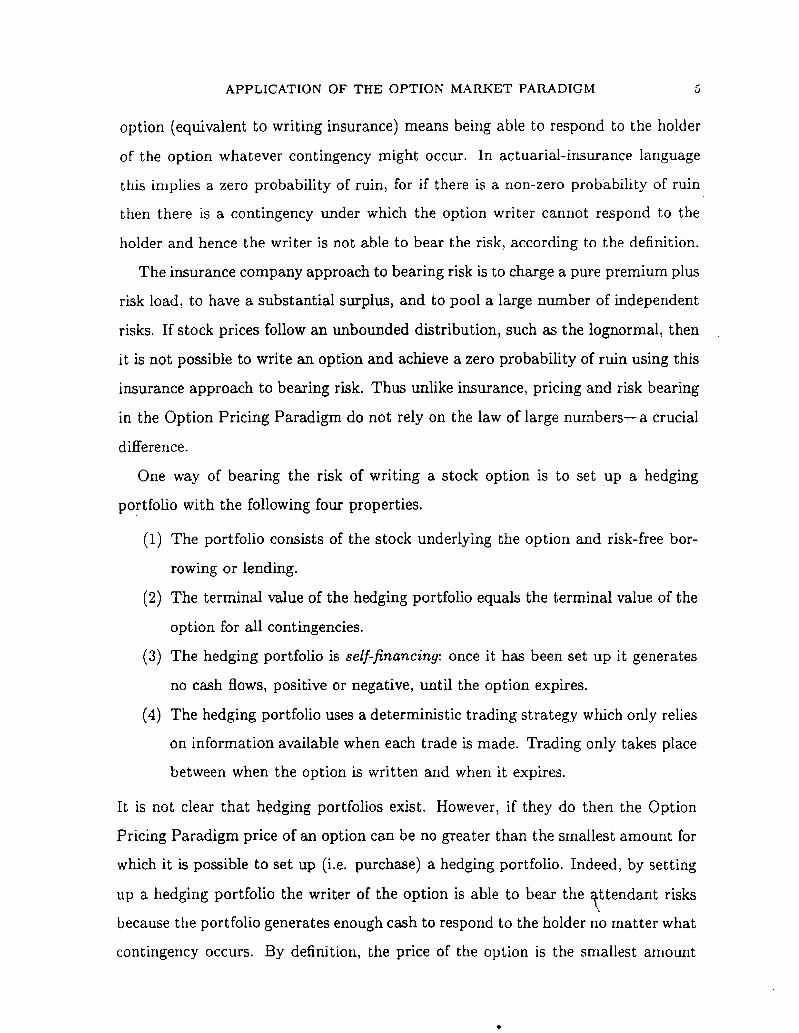
A P P L I C A T I O N OF T H E O P T I O N M A R K E T P A R A D I G M 5

option (equivalent to writing insurance) means being able to respond to the holder

of the option whatever contingency might occur. In actuarial-insurance language

this implies a zero probability of ruin, for if there is a non-zero probability of ruin

then there is a contingency under which the option writer cannot respond to the

holder and hence the writer is not able to bear the risk, according to the definition.

The insurance company approach to bearing risk is to charge a pure premium plus

risk load, to have a substantial surplus, and to pool a large number of independent

risks. If stock prices follow an unbounded distribution, such as the lognormal, then

it is not possible to write an option and achieve a zero probability of ruin using this

insurance approach to bearing risk. Thus unlike insurance, pricing and risk bearing

in the Option Pricing Paradigm do not rely on the law of large numbers--a crucial

difference.

One way of bearing the risk of writing a stock option is to set up a hedging

portfolio with the following four properties.

(1) The portfolio consists of the stock underlying the option and risk-free bor-

rowing or lending.

(2) The terminal value of the hedging portfolio equals the terminal value of the

option for all contingencies.

(3) The hedging portfolio is self-financing: once it has been set up it generates

no cash flows, positive or negative, until the option expires.

(4) The hedging portfolio uses a deterministic trading strategy which only relies

on information available when each trade is made. Trading only takes place

between when the option is written and when it expires.

It is not clear that hedging portfolios exist. However, if they do then the Option

Pricing Paradigm price of an option can be no greater than the smallest amount for

which it is possible to set up (i.e. purchase) a hedging portfolio. Indeed, by setting

up a hedging portfolio the writer of the option is able to bear the }ttendant risks

because the portfolio generates enough cash to respond to the holder no matter what

contingency occurs. By definition, the price of the option is the smallest amount

6 S T E P H E N M I L D E N H A L L

of money for which this is possible. Therefore the actual option price can be no

greater than the cost of the cheapest hedging portfolio.

On the other hand, if there are no arbitrage opportunities, the Option Pricing

Paradigm price must be at least as large as the cost of setting up the cheapest

hedging portfolio. Since the writer can bear the risk of writing the option, they

must have a portfolio, purchased with the proceeds of writing the option, with an

ending cash position at least as large as the terminal value of the option (and hence

a hedging portfolio) in every contingency. Such a portfolio is said to dominate the

hedging portfolio. If portfolio A dominates portfolio B then, in the absence of

arbitrage, A must cost more than B. Here, the option price is used to purchase

a portfolio which in turn dominates a hedging portfolio and therefore the option

price must be at least as great as the cost of a hedging portfolio. 3 Combining this

with the previous paragraph shows that in the absence of arbitrage the Option

Pricing Paradigm price equals the smallest amount for which it is possible to set up

a hedging portfolio.

The above argument relies on the absence of arbitrage opportunities in the mar-

ket. An arbitrage is the opportunity to earn a riskless profit. In general, the

existence of arbitrage opportunities is not compatible with an equilibrium model of

security prices, since informed agents would engage in arbitrage and hence modify

3 I could have simply defined the price of the option to be the smallest cost of

setting up a hedging portfolio. For example, in Karatzas and Shreve [23] the fair

price for a contingent claim is defined as the smallest amount x which allows the

construction of a hedging portfolio with initial wealth x. However, it is generally

not possible for an insurer to set up a hedging portfolio because it cannot trade in

the security underlying the insurance contract option. Thus, a definition in terms

of hedging portfolios would not have transferred to insurance. On the other hand,

"the cost of bearing the risk", albeit with a possibly weaker notion ~f bearing risk,

makes perfect sense in an ir~surance setting and is equivalent to the hedging portfolio

definition for options, which is why I chose it.

A P P L I C A T I O N OF T H E O P T I O N M A R K E T P A R A D I G M 7

market prices (see Dybvig and Ross [16] for an explanation of tile close connections

between no arbitrage and options pricing). In options pricing, no arbitrage is used

to justify defining the price of an option as the smallest cost of a hedging portfolio:

if the option sold for more or less than the cost of a hedging portfolio then risk-free

arbitrage profits would be possible. Put another way, the option and the hedging

portfolio are comparables and no arbitrage implies that comparables must have the

same value. Since "the value of an asset is equal to the combined values of its

constituent items of cash flow" [3] if two assets have the same cash flows then they

are equivalent to an investor and must command the same price. The fact that one

is an option and the other a synthetic option created from a portfolio of bonds and

stocks is irrelevant. Obviously this only applies in a world where the BlackoScholes

assumptions hold--so in particular there are no transaction costs, no discontinuous

jumps in stock prices, and continuous trading. Finally no arbitrage is a conse-

quence of the model framework, not an assumption; potential arbitrages are ruled

out through restrictions on admissible trading strategies. This is a more advanced

point; the interested reader should see Harrison and Kreps [19], Dothan [14], and

Delbaen and Schachermayer [10], [11] and [12] for more detailed information.

To conclude, this section has introduced the notions of no-arbitrage and hedging

portfolios, and explained how the Option Pricing Paradigm defines price to be the

smallest cost of setting up a hedging portfolio. These beginnings are enough to

point out some significant differences compared to actuarial methods of pricing,

one of which is that option pricing does not rely the law of large numbers. The

question of whether hedging portfolios actually exist will be discussed in Section 4.

First, I want to look at how an actuary would price an option.

3. AN ACTUARIAL APPROACH TO OPTION PRICING

It is instructive to compare the Black-Scholes price with the actuarial price.--

including risk load -for a call option. Before defining terms we muslt fix the nota-

tion. Assume all interest rates and returns are continuously compounded. Let r

be the risk free rate of interest, # the expected return on the stock, S(t) or S~ the


stock price at time t, and r' a risk-adjusted interest rate for discounting the option

payouts. To keep the notation as simple as possible, assume that the current time

is t = 0 and that the option expires at time t = T. Assume also that the stock

price process is a geometric Brownian motion, 4 so that log(S(t)/S(O)) is normally

distributed with mean t(# - 32/2) and variance ta 2 for some a > 0. Finally, let k

be the exercise price.

The actuarial price for the option is the present value of the expected payouts

discounted at a risk-adjusted interest rate

e - r ' T E ( ( S ( T ) - k)+). (3.1)

With r' = r Equation (3.1) is Equation (1.3) from the paper. 5 An actuary could

compute Equation (3.1) after estimating appropriate values for #, a and r'. For ju

4 This means that over a very short time interval dt the return on the stock dSt /S t

satisfies the stochastic differential equation dSt /S t = #dr + adWt where Wt is a

Brownian motion. By definition Wt is normally distributed with mean zero and

variance ta 2. It follows from Ito's Lemma that the solution to the stock price

stochastic differential equation can be written as St = So exp((~u - o'2/2)t + o'Wt).

Hence St has a lognormal distribution and log(St~So) is normal with mean (# -

o-2/2)t and variance to 2. Since E(St) = Soe ~t it is reasonable to call p the expected

rate of return on the stock. See Hull [20], or Karatzas and Shreve [23], for more

details. Hull, Chapter 10.3, discusses the difference between expected returns over

a short period of time and the expected continuously compounded rate of return.

If' there is variability in the rate of return, so a > 0, then the former, #, is greater

than the latter, # - o'2/2. 5 Mr. Wacek justifies assuming r ~ = r using the notion of a hedging portfolio.

However, in this section I am taking an actuarial viewpoint and so do not want

to use such a notion. To the ac tuary--and the financial economics community as

whole prior to Black-Scholes--we should have r ' > # > r since the ~ption is more

leveraged than the stock and hence more risky. Brealey and Myers [2] point out

that the option has a higher beta and a higher standard deviation of return than

A P P L I C A T I O N O F THE O P T I O N M A R K E T P A R A D I G M 9

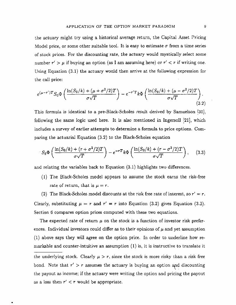
the actuary might try using a historical average return, the Capital Asset Pricing

Model price, or some other suitable tool. It is easy to estimate a from a time series

of stock prices. For the discounting rate, the actuary would mystically select some

number r ' > # if buying an option (as I am assuming here) or r ' < r if writing one.

Using Equation (3.1) the actuary would then arrive at the following expression for

the call price:

e(~_r,)T So ~ ( In (So /k) + +

] e_,.,Tk ¢ (In(So~k) + (# - o.2/2)T~

(3.2) This formula is identical to a pre-Black-Scholes result derived by Samuelson [31],

following the same logic used here. It is also mentioned in Ingersoll [21], which

includes a survey of earlier a t tempts to determine a formula to price options. Com-

paring the actuarial Equation (3.2) to the Black-Scholes equation

(In(So~k) + (r + a2/2)T + (r- a2/2)T ax/~ ) -e-rTk~ (ln(S°/k) ~ " ) , (3.3) P S0 ~

and relating the variables back to Equation (3.1) highlights two differences.

(1) The Black-Scholes model appears to assume the stock earns the risk-free

rate of return, that is # = r.

(2) The Black-Scholes model discounts at the risk free rate of interest, so r ' = r.

Clearly, substi tuting # = r and r ' = r into Equation (3.2) gives Equation (3.3).

Section 6 compares option prices computed with these two equations.

The expected rate of return # on the stock is a function of investor risk prefer-

ences. Individual investors could differ as to their opinions of # and yet assumption

(1) above says they will agree on the option price. In order to underline how re-

markable and counter-intuitive an assumption (1) is, it is instructive to translate it

the underlying stock. Clearly/z > r, since the stock is more risky than a risk free

bond. Note that r ' > r assumes the actuary is buying an option a id discounting

the payout as income; if the actuary were writing the option and pricing the payout

as a loss then r ' < r would be appropriate.

L0 STEPHEN MILDENHALL

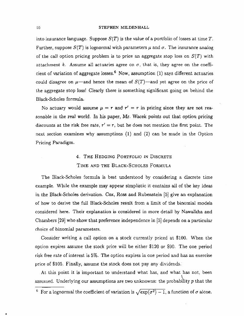
into insurance language. Suppose S(T) is the value of a portfolio of losses at time T.

Further, suppose S(T) is lognormal with parameters # and a. The insurance analog

of the call option pricing problem is to price an aggregate stop loss on S(T) with

at tachment k. Assume all actuaries agree on a, that is, they agree on the coeffi-

cient of variation of aggregate losses. 6 Now, assumption (1) says different actuaries

could disagree on ~ - - a n d hence the mean of S ( T ) - - a n d yet agree on the price of

the aggregate stop loss! Clearly there is something significant going on behind the

Black-Scholes formula.

No actuary would assume # -- r and r I -- r in pricing since they are not rea-

sonable in the real world. In his paper, Mr. Wacek points out that option pricing

discounts at the risk free rate, r ' -- r, but he does not mention the first point. The

next section examines why assumptions (1) and (2) can be made in the Option

Pricing Paradigm.

4. THE HEDGING PORTFOLIO IN DISCRETE

TIME AND THE BLACK-SCHOLES FORMULA

The Black-Scholes formula is best understood by considering a discrete time

example. While the example may appear simplistic it contains all of the key ideas

in the Black-Scholes derivation. Cox, Ross and Rubenstein [5] give an explanation

of how to derive the full Black-Scholes result from a limit of the binomial models

considered here. Their explanation is considered in more detail by Nawalkha and

Chambers [29] who show that preference independence in [5] depends on a particular

choice of binomial parameters.

Consider writing a call option on a stock currently priced at $100. When the

option expires assume the stock price will be either $120 or $90. The one period

risk free rate of interest is 5%. The option expires in one period and has an exercise

price of $105. Finally, assume the stock does not pay any dividends.

At this point it is important to understand what has, and what has not: been

assumed. Underlying our assumptions are two unknowns: the probabhity p that the

6 For a lognormal the coefficient of variation is x/exp(a 2) - 1, a function of a alone.

A P P L I C A T I O N OF THE O P T I O N M A R K E T P A R A D I G M 11

stock price will end at $120, and an expected return ~u on the stock. The expected

return ~a is

~ = l°g ( 120p + 9 0 ( 1 - p)

(using continuous compounding) or, equivalently

$100 = e-~(120p + 90(1 - p)). (4.1)

Equation (4.1) expresses the current price as an expected present value, discounted

at a risk adjusted interest rate. It gives one relationship between the two unknowns p

and #. It is impossible for us to know whether the current stock price is $100 because

there is a very good chance of an upward price movement (high p) but investors are

all very risk averse (giving a high #), or because there is only a moderate chance

of an upward movement in a largely risk neutral market. The fact that the Black-

Scholes formula is independent of the choice of # and p, subject to the constraint

Equation (4.1), is one of its most remarkable features and it leads to the notion of

risk-neutral valuation.

Return now to pricing the $105 call option under the Option Pricing Paradigm.

From Section 2, the price of the call is the smallest cost for which it is possible to

set up a hedging portfolio. I will now construct an explicit hedging portfolio for

the option, demonstrat ing that they exist, at least in this simple case. Suppose the

hedging portfolio consists of a stocks and $b in bonds. The replicating property of

a hedging portfolio requires that, at expiration,

120a + b = 15

90a + b = 0.

The top line corresponds to an upward movement in the stock price, when the option

is worth m a x ( 1 2 0 - 105, 0) = 15 at expiration. The bot tom line corresponds to a

downward movement in the stock price, when the option is worth maxx(90-105, 0) =

{). Solving gives a = 1/2 and b = -$45, meaning borrow $45. The cost today of

setting up a portfolio which consists of half of one stock plus $45 debt one period

12 STEPHEN MILDENHALL

from now equals 100/2 -- e-°°545 = $7.19. The first term is tile cost of buying tlalf

a stock and the second term is the present value of a debt of $45 one period from

now.

It is easy to confirm this portfolio hedges the option. If the stock price moves

up, then selling the half-stock yields $60, exactly enough to pay off the $45 debt

and pay the owner of the option the $15 terminal value. If the stock price moves

down then selling the half-stock realizes $45, which is exactly the amount required

to pay off the debt. There is nothing else to pay since the option expires worthless.

Using the hedging portfolio it is also easy to see why no arbitrage implies $7.19

is the appropriate price for the option. If the option sold for more than $7.19,

say $7.25, then arbitrageurs would write (sell) the over-priced options. With $7.19

of the proceeds they could set up a hedging portfolio, effectively closing out their

option position. They would make a risk free profit of $0.06 per option written.

On the other hand, suppose the option sold for only $7.15. Then arbitrageurs

would want to buy the under-price options. They could short one stock to get $100,

and use the proceeds to buy 2 options for $14.30, put $85.61 into bonds earning

the risk free rate, and skim off the remaining 9 cents as arbitrage profit. If the

stock price rises to $120, they exercise the two options to yield a $30 profit which

combined with $85.61e °°5 = $90 in bonds gives $120--exactly enough to close out

the short position in the stock. If the stock price falls to $90 then the options

expire worthless but the arbitrageurs still have $90 in the bonds to close to the

stock position.

To summarize, these arguments lead to essentially the same two conclusions

already noted in Section 3 from comparing Black-Scholes and the actuarial option

price.

(1) The option price is $7.19 regardless of the risk preferences of individuals,

expressed through the unknown quantities # and p, provided Equation (4.1)

is satisfied.

(2) The hedging portfolio consists of stock and risk-free borrowing only. Once it

is set up there is no risk to the option writer because movements in the stock


price and the option price are perfectly correlated. A portfolio consisting

of the hedge and the underlying option must therefore earn, and hence be

discounted at, the risk free rate of return.

Black and Scholes showed these two results are still true when the stock price is

allowed to follow a more complex path in continuous time. Under the lognormal

stock price assumption, they proved the option price function is given by Equation

(3.3), and derived the required trading strategy to use in the hedging portfolio--the

so-called "delta-hedging" strategy.

Cox and Ross [4] used the risk preference independence in (i) to argue that an

option could be priced assuming investors have any convenient risk preference. The

simplest selection for preferences is risk-neutrality. In a risk-neutral world all stocks

are expected to earn the risk free return because investors do not require a premium

for uncertainty. Thus # -- r is determined. Of course, stocks do not earn the risk

free return in the real, risk-averse, world. In our simple discrete model, selecting

risk-neutral preferences for investors is equivalent to setting # -- r so now we can

solve Equation (4.1) for p, to get/5 = (100e r - 90)/30 = 0.50424. A similar result

holds in continuous time: it is possible to explicitly adjust the stock price process to

that which would prevail in a risk neutral world. The adjusted process is denoted

S(t). ,~(T) and S(T), the distribution of the actual stock price at time T, will be

different since the risk-neutral assumption does not hold in the real world.

The adjustment that takes S to S is an adjustment of underlying probabilities.

Risk preferences can be understood as a subjective assessment of probabilities for

future events. Pdsk-averse individuals will assign greater than actual probability to

bad outcomes. The adjustment we are looking for will be an assessment of these

subjective probabilities. In order to reduce the return on a stock from # to r the

probability of bad outcomes is increased and the probability of good outcomes is

decreased. The adjusted probabilities are called an equivalent martipgale measure

because the discounted stock price process becomes a martingale with respect to

the new probabilities.


Wang's proportional hazard transform method for computing risk loads also

works by altering probabilities see [34], [35]. For this reason I believe that Wang's

method is in line with modern financial economic thinking and deserves serious

consideration by actuaries.

In a risk-neutral world an option will be valued as the present value of its expected

payouts, discounted at the risk-free rate. For a call option with exercise price k this

would be

e-rTE((5 ' (T)-k)+).

Equation (4.2) gives a pricing formula very similar to the author 's equation

(4.2)

e - rTE( (S (T) -k )+) . (4.3)

The difference between the two is the use of S, the real stock price process, versus

,.~, the process that holds in a risk-neutral world. S will have an expected return

equal to r < # and is certainly different from S the "probability distribution of

market prices at expiry" which Mr. Wacek uses in his version of Equation (4.3)

on page 703. Section 6 gives a comparison of prices from these two formulae with

actual market prices.

Finally, it is now clear that the Black-Scholes formula gives a price rather than

a pure premium. Once the hedging portfolio has been set up there is no risk to the

option writer; therefore there is no need for a risk load. In fact, adding a risk load

to the Black-Scholes price would create an arbitrage opportunity. Mr. Wacek makes

this point in his footnote 2, but then obscures the issue by characterizing the rate

as a pure premium to allow for an extra risk load when the hedging argument is not

available. However, he does not discuss what conditions are necessary in order to

use a hedging argument. It turns out the condition is precisely that there exists an

equivalent martingale measure, as discussed above. See Duffle [15] for more details

on this point. Also, see Gerber and Shiu [17], Cox and Ross [4] and Delbaen et al.

[13] for a discussion of pricing options based on stock price processes gther than the

lognormal used in Black-Scholes.


5. T w o ACTUARIAL APPLICATIONS OF THE OPTION PRICING PARADIGM

Catastrophe Insurance

I believe the Option Pricing Paradigm view is useful in a situation where Black-

Scholes will likely never apply: catastrophe insurance and reinsurance pricing. It

tells us to price by computing the cost of being able to bear the risk for the contract

period and not by loading the expected loss for risk. For catastrophe reinsurance

this means having access to a large, liquid pool of cash. The Option Pricing Par-

adigm also tells us to move away from a "bank" mentality where reinsurance is

providing inter-temporal smoothing and consider the premium spent during the ex-

posure period on bearing the risk. Most other lines of insurance are based on such a

point-in-time, between-insured risk sharing, rather than inter-temporal, per-insured

risk sharing. As noted in Jaffee and Russell [22] many institutional problems arise

for catastrophe insurance precisely because of the inter-temporal way it is currently

handled.

Using the Black-Scholes model, the writer of an option uses the option premium

to maintain the hedging portfolio (the hedging trading strategy for a call is buy

high, sell low, so it is guaranteed to lose money). When the option expires the initial

premium has been exactly used up in stock trading losses whether the option ends

up in or out of the money. Similarly, working within this framework, a catastrophe

insurance premium should be spent during the policy term, perhaps on maintaining

a line of credit, or paying a higher than market interest rate on a cat-bond.

Interestingly, it does not make sense to ask for a contingency reserve with this

viewpoint, for two reasons. Firstly because at the end of the contract period there

is no remaining premium to put into a reserve, and secondly because there is little

or no taxable income produced by the product. The need for catastrophe reserves is

largely a product of taxation of insurance companies. In this model the catastrophe

risk and premium would pass through the insurance company to a~n entity, such

as a hedge [und, more economically suited to bearing the risk and providing the

necessary funding after a large event.


Options on Non-Traded Ins t ruments

The Black-Scholes approach appears to rely on the possibility of taking a position

in the underlying stock. This is partially true. More important, however, is the fact

that the stock represents the only source of uncertainty, or stochastic behavior, in

the system. Writing an option and maintaining a hedging portfolio cancels out the

pricing uncertainty, leaving a risk free portfolio--as discussed above.

Consider an option on an untraded quantity, such as interest rates or an insur-

ance loss index. While, by definition, it is not possible to take a position in the

underlying, there is still only one source of uncertainty. Therefore, a Black-Scholes

type argument can be used to construct a risk-free portfolio consisting of two op-

tions with different exercise prices or expiration dates. The portfolio will use the

fact that the two options have instantaneously perfectly correlated prices to cancel

all the risk (stochastic behavior). The result is a partial differential equation similar

to the Black-Scholes equation involving the prices of the two options as unknowns.

Unfortunately one equation between two unknowns does not give a unique solution.

(When the underlying is traded its price is known already, giving one equation in

one unknown, which is soluble.) However, the partial differential equation can be

separated into an expression of the form

f(C~)= f(C2)

for some function f , where C1 and C2 are the unknown option prices. Since the

left hand side depends on the expiration and exercise price of C1 but not C2, both

sides must be a function of the risk free rate r and time t alone. This implies

there are Black-Scholes-like partial differential equations for the prices of C1 and

C2 each with one extra unknown, called the market price of risk for the underlying

index. Since all the option prices depend on the same extra parameter, there are

strong consistency conditions put on the prices of a set of options on one underlying

instrument. This approach could be useful in an insurance context \ to help price

derivatives off an insurance-based index. For a more detailed explanation of how

the approach is applied to price interest rate derivatives, see Wilmot et al., [36].


6. BLACK-SCHOLES 1N ACTION

How well does the Black-Scholes formula perform in practice? It is often asserted

that the model is widely used in the industry and also that traders are aware of

its weaknesses; it is rarer to see comparisons with market prices. In this section I

want to give such a comparison. This is not a scientific test of the model; rather it

is supposed to indicate roughly how well it performs.

The table below gives the closing prices for all December S&P 500 European call

options on September 15, 1997. The calls expired on December 19, 1997. The risk

free force of interest was about 5.12% giving a discount factor of 0.9868. The S&P

500 closed September 15 at 919.77.

TABLE 1

BLACK SCHOLES PRICES

Exercise Market Traded Intrinsic BS Percent Implied Actuarial Price Price Volume Value Price Error o" Price

750 186 714 169.77 181.06 -2.7% 32.83% 201.98 805 135 3 114.77 130.90 -3.0 27.92 150.55 890 67 1/2 10 29.77 66.89 -0.9 23.86 82.04 900 64 6 19.77 60.88 -4.9 25.27 75.32 910 59 1/4 102 9.77 55.21 -6.8 25.73 68.93 930 44 1/4 3,291 0.00 44.96 1.6 23.12 57.18 935 41 3/4 5 0.00 42.62 2.1 23.04 54.46 940 42 1/2 264 0.00 40.36 -5.0 24.64 51.83 950 36 1/4 14 0.00 36.11 -0.4 23.57 46.82 960 31 1/2 2 0.00 32.20 2.2 23.12 42.16 990 21 5 0.00 22.37 6.5 22.69 30.19 995 20 107 0.00 20.98 4.9 22.91 28.48 ,025 11 7 0.00 14.07 27.9 21.28 19.71

The market price shows the last trade price for each option. The intrinsic value

is given by the current index price minus the exercise price, if positive. The Black-

Scholes formula price (BS Price) is computed using a = 23.50%, an estimate derived

from a contemporaneous sample of S&P daily returns. The implie~l volatility is

calculated by setting the Black-Scholes price equal to the market price and solving

fbr a. The actuarial price is computed using Equation (3.2) with r ~ = r, tile risk


t'ree rate of return and # = 13.98% for a 15% annual return. Assuming r ' = r makes

my Equation (3.2) exactly the same as formula (1.3) on page 703 of the paper for

a lognormal stock price distribution. Thus the last column shows the impact on

the option price of using the approximate expected rate of return of the underlying

instrument rather than the risk free rate of return; this is the difference between

using S and S as the stock price process. Clearly market prices are much closer to

the Black-Scholes price. Using a higher discount rate in place of r, but leaving #

unchanged would bring the actuarial price closer to the Black-Scholes value.

The results are really quite spectacular, especially when compared to the range

of reasonable values determined by m a n y actuarial analyses. Remember there is

only one free parameter underlying all the model values, and even that is easy to

estimate. As Hull [20] points out, the last option trade may have occurred well

before the market closed, so the option price may correspond to a different S&P

index value than the close. Hull is also a good reference for more information on

the mechanics of options markets and for reasons why market prices diverge from

Black-Scholes prices.

Finally, Table 1 only provides evidence that the market prices using Black-Scholes

or a very similar formula. It does not necessarily follow that ttfis is the "correct"

price!

7. CONCLUSION

The thrust of Mr. Wacek's paper is that options pricing and insurance pricing are

essentially the same and that it should be possible for each discipline to learn from

the other. In many ways this is true, particularly on a practical level. Examples

include the author 's sections on rate guarantees and multi-year contracts. The

philosophy of "look for the option" is an important part of modern finance, and is

well illustrated by the many applications in Brealey and Myers [2]. Given its central

role in finance, actuaries should understand the Option Pricing Part~digm arid be

able to apply it, where relevant, in their own work. Mr. Wacek's paper is valuable

because helps point actuaries in this direction.

A P P L I C A T I O N OF THE O P T I O N M A R K E T P A R A D I G M 19

I would, however, argue that there are some very significant differences between

the Option Pricing Paradigm and insurance which should not be glossed over. The

Option Pricing Paradigm is based on arbitrage and pricing comparables, and it relies

on hedging to remove risk. Insurance assumes and manages specific risk, (Turner

[33]). There are typically no liquid markets or close comparables for the specific

assets underlying insurance liabilities and so option pricing techniques do not apply. ~

The specialized underwriting knowledge that insurance companies develop is a key

part of their competitive advantage; what they do is bear the resulting underwriting

risk, they do not hedge it away. s This point is discussed by Santomero and Babbel

[32] in their review of financial risk management by insurers. Obviously, how an

individual company chooses to manage risk does not alter the market price; the

existence of a hedge-based pricing mechanism does, however, determine a market

price in the absence of arbitrage.

At a detailed level, I do not agree with how Mr. Wacek has gone from the

Black-Scholes formula to his supposedly more general Equation (1.3) (Equation

(,.1.3) here). I have shown how an actuarial approach to option pricing produces a

result similar to the Black-Scholes formula but with two important differences: the

assumed return on the stock (expected market return compared to risk free return)

and the discount rate (a rate greater than the expected market return compared

to the risk free return). The Black-Scholes argument shows that writing options is

risk-free (in the conceptual model) because of the possibility of setting up a self-

financing hedging strategy with the proceeds from writing an option. No arbitrage

then implies the price of the option must be the smallest amount for which it is

possible to set up a hedging portfolio. It follows that the option price is independent

of individual investor's risk preferences. Cox and Ross then argued that the option

As Babbel says in [1]: "When it comes to the valuation of insurance liabilities,

the driving intuition behind the two most common valuation approaches--arbitrage

and comparables--fails us." s Unless they can use their specialized knowledge to arbitrage the reinsurance

markets!

20 S T E P H E N MILDENHALL

can be priced assuming risk-neutrality. In a risk-neutral world stocks earn the risk

free return, thus explaining the first assumption. The hedging portfolio argument

also shows the risk free rate is appropriate for discounting, which explains the second

assumption. Mr. Wacek makes the latter point but does not mention the former. As

shown in Table 1 there is a significant difference between the option prices with and

without the former assumption. Moreover, market prices are consistently closer to

the Black-Scholes prices. The discussion of hedging and options pricing also makes

it clear Black-Scholes gives a price, not a pure premium. Finally, Mr. Wacek's

assertion "the pricing mathematics is basically the same" for options and insurance

is not really the case. Doubts as to this point can be dispelled by looking in any

more advanced text on options pricing, such as [14].

In this review I have given a simple discrete time example to illustrate the hedging

portfolio argument. It shows how the option price is independent of risk preferences

given the current stock price. While the example is often reproduced in finance texts

I believe the discussion of exactly how risk preferences fit in, through Equation (4.1),

is less common. I proposed a new application of the Option Pricing Paradigm to

catastrophe insurance, and discussed how the paradigm works in the case of an

underlying which is not traded. Finally, I gave a comparison of market prices,

Black-Scholes prices and actuarial prices for some S&P options.

The Black-Scholes option pricing formula is an important and beautiful piece

of mathematics and financial economics. On the surface the formula is just the

discounted expected excess value of a lognormal random variable--the tricky part

is which lognormal variable! Understanding some of the paradigm lying behind the

formula, and some of its subtleties, gets us to the core of the differences between how

insurers and other financial institutions bear and manage risk. Given the current

convergence between insurance and banking it is important for insurance actuaries

to understand and to be able to exploit these differences .... our future livelihood

could depend upon it.


REFERENCES

[1] Babbel. David F., Review of Two Paradigms for the Market Value of Liabilities by R. R. Re- itano, North American Actuarial Journal 1(4) (1997), 122-123.

[21 Brealey, Richard A. and Stewart C. Myers, Principles of Corporate Finance, 4th Edition, McGraw-Hill, 1981.

[3] Casualty Actuarial Society, Statement of Principles Regarding Property and Casualty Valua- tions, as adopted September 22, 1989 (1997), Casualty Actuarial Society Yearbook, 277-282.

[4] Cox, d. and S. Ross, The Valuation of Options for Alternative Stochastic Processes, Journal of Financial Economics 3 (1976), 145-166.

[5] Cox, J., S. Ross, and M. Rubenstein, Option Pricing: A Simplified Approach, Journal of Financial Economics 7 (1979), 229-263.

[6] Cummins, J. David, Risk-Based Premiums for Insurance Guarantee Funds, Journal of Fi- nance 43 (1988), 823-839.

[7] Cummins, J. David and H~lyette Geman, An Asian Option Approach to the Valuation of Insurance Futures Contracts, Review of Futures Markets 13(2) (1994), 517-557.

[8] _ _ , Pricing Catastrophe Insurance Futures and Call Spreads: An Arbitrage Approach, J. of Fixed Income 4(4) (1995), 46-57.

[9] D'Arcy, Stephen P. and Neil A. Doherty, The Financial Theory of Pricing Property Liability Insurance Contracts, Huebner Foundation/Irwin, Homewood IL, 1988.

[10] Delbaen, F. and W. Schachermayer, A General Version of the Fundamental Theorem of Asset Pricing, Math. Ann. 300 (1994), 463-520.

[11] _ _ , Arbitrage possibilities in Bessel processes and their relation to local martingales, Probability Theory and Related Fields 102 (1995), 357-366.

[12] _ _ , Arbitrage and Free Lunch With Bounded Risk for Unbounded Continuous Processes, Mathematical Finance 4(4) (1994), 343-348.

[13] Delbaen, F., W. Schachermayer and M. Schwizier, Review of Option Pricing by Esscher Transforms, Transactions of the Society of Actuaries XLVI (1994), 148-151.

[14] Dothan, Michael U., Prices in Financial Markets, Oxford University Press, 1990. [15] Duffle, Darrell, Dynamic Asset Pricing Theory, Princeton University Press, 1992. [16] Dybvig, Philip H. and Stephen A. Ross, Arbitrage, The New Palgrave: Finance (J. Eatwell,

M. Milgate and P. Newman, eds.), W.W. Norton, 1987, pp. 57-71. [17] Gerber, Hans U. and Elias S.W. Shiu, Option Pricing by Esscher Transforms, Transactions

of the Society of Actuaries XLVI (1994), 99-191. [18] Gillam, William R. and Richard H. Snader, Fundamentals of Individual Risk Rating, National

Council on Compensation Insurance, 1992. [19] Harrison, J.M. and D. Kreps, Martingales and Arbitrage in Multiperiod Securities Markets,

Journal of Economic Theory 20 (1979), 381-408. [20] Hull, John C., Options Futures and Other Derivative Securities, Second Edition, Prentice-

Hall, 1983. [21] Ingersoll Jr., Jonathan E., Options Pricing Theory, The New Palgrave: Finance (J. Eatwell,

M. Milgate and P. Newman, eds.), W.W. Norton, 1987, pp. 199-212. [22] Jaffee, Dwight M. and Thomas Russell, Catastrophe Insurance, Capital Markets, and Unin-

surable Risks, Journal of Risk and Insurance 64(2) (1997), 205-230. [23] Karatzas I. and S. Shreve, Brownian Motion and Stochastic Calculus, Springer-Verlag, New

York, 1988. [24] Kellison, Stephen G., The Theory of Interest, 2nd Edition, Irwin, 1991. [25] Lee Y. S., The Mathematics of Excess of Loss Coverage and Retrospective Rating--A Graph-

ical Approach, Proceedings of the Casualty Actuarial Society L X X V (1988), 49-77. [26] , On the Representation of Loss and Indemnity Distributions, Prc~ceedings of the

Casualty Actuarial Society L X X V I I (1990), 204-224. [27] Mcrton, Robert C., Theory of Rational Option Pricing, Continuous Time Finance, Blackwell,

1990.


[28] Miccolis, Robert S., On the Theory of Increased Limits and Excess of Loss Pricing, Proceed- ings of the Casualty Actuarial Society L X I V (1977), 27-59.

[29] Nawalkha. Sanjay K. and Donald R. Chambers, The Binomial Model and Risk Neutrality: Some Important Details, The Financial Review 30(3) (1995), 605-615.

[30] Phillips, Richard D., J. David Cummins and Franklin Allen, Financial Pricing of Insurance in the Multiple-Line Insurance Company, The Journal of Risk and Insurance 65(4) (1998). 597-636.

[31] Samuelson, P.A., Rational theory of warrant pricing, Industrial Management Review 6(2) (1965), 13-32.

[32] Santomero, Anthony M., and David F. Babbel, Financial Risk Management by Insurers: An Analysis of the Process, Journal of Risk emd Insurance 64(2) (1997), 231-270.

[33] Turner, Andrew L., Insurance in an Equilibrium Asset-Pricing Model, Fair Rate of Return in Property-Liability Insurance (J. David Cummins and Scott A. Ha.rrington, eds.), Kluwer- Nujhoff, Boston, 1987.

[34] Wang, S., Premium calculation by transforming the layer premium density, ASTIN Bulletin 2 6 (1995), 71-92.

[35] , Ambiguity-aversion and the economics of insurance, Proceedings of the Risk Theory Seminar, Wisconsin-Madison (1996).

[36] Wilmot, Paul, Sam Howison, and Jeff Dewynne, The Mathematics of Financial Derivatives, A Student Introduction, Cambridge University Press, 1995.

wacekfinal

February 6, 2000 (696)

APPLICATION OF THE OPTION MARKET

Documents

Transcript of APPLICATION OF THE OPTION MARKET