Application of the Bernoulli Enthalpy Concept to the … of the Bernoulli Enthalpy Concept to the...

NASA Contractor Report 2987

Application of the Bernoulli Enthalpy Concept to the Study of Vortex ‘Noise and Jet Impingement Noise

John E. Yates

CONTRACT NASJ-14503 APRIL 1978

https://ntrs.nasa.gov/search.jsp?R=19780014918 2018-06-30T00:52:41+00:00Z

I -

NASA Contractor Report 2987

Application of the Bernoulli Enthalpy Concept to the Study of Vortex Noise and Jet Impingement Noise

John E. Yates Aeromuticd Research Associates of Pritlceton, Ix. Primeton, New Jersey

Prepared for Langley Research Center under Contract NASI-14503

National Aeronautics and Space Administration

Scientific and Technical Information Office

1978

TECH LIBRARY KAFB, NM

-- -

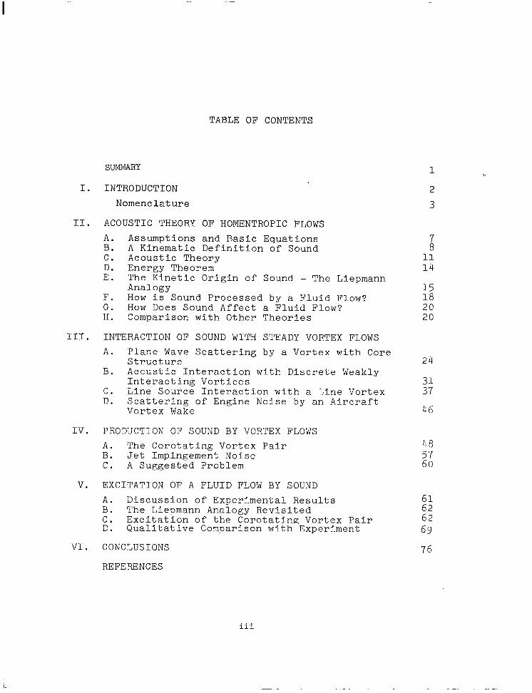
TABLE OF CONTENTS

SUMMARY 1

I. INTRODUCTION 2 Nomenclature 3

II. ACOUSTIC THEORY OF HOMENTROPIC FLOWS A. Assumptions and Basic Equations B. A Kinematic Definition of Sound C. Acoustic Theory D. Energy Theorem E. The Kinetic Origin of Sound - The Liepmann

Analogy F. How is Sound Processed by a Fluid Flow? G. How Does Sound Affect a Fluid Flow? H. Comparison with Other Theories

III. INTERACTION OF SOUND WITH STEADY VORTEX FLOWS A. Plane Wave Scattering by a Vortex with Core

Structure B. Acoustic Interaction with Discrete Weakly

Interacting Vortices C. Line Source Interaction with a ‘,ine Vortex D. Scattering of Engine Noise by an Aircraft

Vortex Wake

IV. PRODUCTION OF SOUND BY VORTEX FLOWS A. The Corotating Vortex Pair B. Jet Impingement Noise C. A Suggested Problem

V. EXCITATION OF A FLUID FLOW BY SOUND A. Discussion of Experimental Results B. The Liepmann Analogy Revisited C. Excitation of the Corotating Vortex Pair D. Qualitative Comparison with Experiment

VI. CONCLUSIONS

L4 11 14

15 18 20 20

24

48

2:

2 62 69

76

REFERENCES

iii

John E. Yates

Aeronautical Research Associates of Princeton, Inc. 50 Washington Road, Princeton, New Jersey 08540

SUMMARY

A general theory of aeroacoustics of homentropic fluid media is presented. The definition of sound (unsteady compressible flow) and the concept of Bernoulli enthalpy are the fundamental building blocks of the theory. It is proved that a Coriolis acceleration is necessary to obtain a transfer of energy from the vertical to the acoustic mode. The Liepmann pendulum is used to illustrate the physical mechanism of noise production by a fluid flow. The basic theory is compared with several known aeroacoustic theories. With the Lighthill hypothesis,the theory is formally equivalent to the Lighthill or Ribner theory in the low Mach number limit. The present theory is complete in that all of the basic aeroacoustic interactionscan be investigated, in particular, the excitation of a fluid flow by sound.

The interaction of sound with vortex flows is studied in detail. A formula for vortex core scattering is derived with a plane wave analysis. A general theory of acoustic interaction with multiple weakly interacting line vortices is presented. The theory is applied to estimate the interference noise between an engine and an aircraft vortex wake. For the DC-9 in a standard take-off configuration the interference noise is estimated to be 3 or 4 DB at the engine peak Strouhal number, for a ground plane observer.

The noise produced by a corotating vortex pair is calculated with the present theory. For low Mach number (M < 0.1) the sound power varies as MT in accordance with known results for compact 2-D flows. For 0.1 < M < 0.3, the power radiated is 10 to 15 DB less than the compact M7 law, even though the basic source is still quadrupole. For M> 0.3, higher order multipoles contribute to the sound power.

An estimate of jet impingement noise is given. It is shown that the acoustic overpressures are a result of acceleration of turbulent eddies through the curved flow near the impingement point. The conventional shear noise term is amplified by a factor of 3 that translates into a factor of 9 (" 10 DB) in the sound power. Our estimates are in agreement with the order of magnitude of recent

measurements. The corotating vortex model or its extension to ring vortices is suggested as a dynamic model of the jet impingement problem.

The phenomenon of fluid flow excitation by sound is investigated. When plane waves impinge on the corotating vortex pair, resonant excitation or attenuation is possible. The coupling is a maximum when the acoustic excitation frequency is approximately twice the rotational frequency of the pair. The wave length can be quite large compared to the separation of the vortices. Based on our simple model,a qualitative explanation of various experimental observations with excited jets is offered.

I. INTRODUCTION

In Ref. l,we presented a comprehensive theory of aeroacoustics that departs in several fundamental ways from the more familiar theories of Lighthill (Ref. (Ref. 4).

21, Ribner (Ref. 3) and Lilley Since the original paper was presented, numerous problems

have been solved (see Ref. 5 and work reported herein). Based on these results and discussions with various people involved in aeroacoustics research,we have been able to modify and polish the original concepts. The basic theory and its application to several problems of technological importance is the subject of this report.

In Section II, we give a detailed derivation of the theory for the case of constant entropy (homentropic) flows. The basic concepts are most easily presented for this case and the resulting theory is directly applicable to a variety of important problems. Three basic questions of aeroacoustics are posed and discussed in the light of the present work and previous theories:

1. How is sound produced by a "primary" fluid flow?

32: How is sound processed by a flow? How does sound affect a primary flow?

In Section III, we consider in detail the question of how sound is processed by vortex flows. First, we investigate the importance of vortex core structure by considering the scattering of plane waves from a single vortex. A general formula for the core derived.

scattering is A Lagrangian approach is used to calculate the scattering

of an arbitrary sound field from a set of discrete weakly-interacting line vortices. The special case of a line acoustic source is calculated in detail and used to estimate the scattering of engine noise from an aircraft vortex wake. Specific application is made to the DC-9 where it is estimated that acoustic overpressures of 3 or 4 DB can result from the interference between the engine and wake.

In Section IV, we consider the production of sound by vortex flows. First, we consider the model problem of a corotating vortex pair and calculate the effects of noncompactness on the sound

2

radiated. Next, we consider the problem of jet impingement noise. The shear noise source term is calculated for a turbulent stagnation point flow. It is estimated that the convective acceleration of turbulent eddies Tn the curved stagnation point flow can pro-. duce some 10 DB more noise than a free jet. It is suggested that the spinning vortex pair (or vortex rings) could be used to model the impingement problem.

In Section V, we consider the difficult question of how sound affects a fluid flow. The interaction of sound with the spinning vortex pair is used to illustrate the basic phenomena. It is shown that the vortex motion can be excited or deexcited by sound at the acoustic frequency of the vortex (twice the rotational frequency). The results are in qualitative agreement with experimental results on excited jets.

NOMENCLATURE

a

A

Am

Bm

cn

DB

E

F(R,ct)

h

H

H

H;')(z)

H(x)

LS,S

isentropic sound speed

Lagrange coordinate of line vortex, see Eq. (3.43)

see Eq. (3.64)

see Eq. (3.65)

amplitude of multipoles in vortex noise, see Eqs. (4.23) and (4.25)

decibel

kinetic energy of primary flow, see Eq. (2.31)

source function for corotating vortex pair, see Eq. (4.11) and Fig. 4.2

enthalpy

h + v2/2

Bernoulli Enthalpy, see Eq. (2.19)

Hankel function of first kind

HeaviSide Step fUnCtiOn

Cartesian unit vectors, see Fig. 3.1

3

1

I

Jn k

M

P

P

rcsre3 b/3

-t 5 rO

r,e

R

S

s,P>

S,(R)

t -t U

ii +;

2 + va V (r) -t X

x,y 'n

c1

Y

acoustic intensity

Bessel function Of the first kind

wave number, ~IT/A

Mach number

pressure

sound power, see Eq. (4.29)

length scale of solid body, exponential and Betz cores, see Eq. (3.38)

unit vector

see Fig. 4.1

plane polar coordinates

normalized radius vector, see Eq. (4.8)

scattering factor, see Eq. (3.27)

core scattering factor, see Eq. (3.24)

see Eqs. (4.18) and (4.19)

time

nonacoustic velocity

mean and turbulent velocity component in a turbulent flow

velocity vector

acoustic particle velocity

velocity distribution in vortex, see Eq. (3.1)

position vector

see Eq. (5.7)

Bessel function of the second kind

see Eq. (4.8)

r/21~ modified vortex strength (also ratio of specific heats)

4

r

ri jk 6(Y)

&h,b,6p

E

K

x -.

% V

P

T,T

9

X

w -t w

II,

R

Q(r)

total vortex strength, see Eq. (3.25)

Christoffel symbol, see Eq. (4.38)

Delta function

perturbation enthalpy, pressure, density

see Eq. (5. 9)

kro , see Eq. (5.6)

wave length of sound, 2r/k

vortex acoustic length scale, see Eq. (3.31)

kinematic viscosity

density

dimensionless time

acoustic potential

vortex potential

radian frequency

curl f , vorticity

streamfunction

angular velocity of corotating vortex pair

vortex core vorticity distribution

Special Notation

curl curl operation

div divergence operation

D Dt substantive derivative $& + ?-grad

D Dt

& + t-grad

grad gradient operation

<(I' time average of any quantity q

5

Tm Re

Im

V2

absolute value of vector ;;

see Eq. (3.63)

real part of complex quantity

imaginary part of complex quantity

Laplace operator

6

II. ACOUSTIC THEORY OF HOMENTROPIC FLOWS

A. ASSUMPTIONS AND BASIC EQUATIONS

We consider the class of aeroacoustic problems for which we can justifiably ignore real fluid properties that lead to significant entropy variations; e.g., the generation of heat by viscous dissipation of mechanical turbulent energy and the production of entropy by internal conduction of heat or by nonadiabatic processes at a boundary. Clearly, our assumption of homentropic flow imposes an upper bound on the Mach number and temperature gradients in the flow. Generally speaking we will be concerned with low to moderate subsonic Mach numbers and the interaction between two of the fundamental modes of energy transport in a fluid (Ref.. 6):

1) The acoustic mode 2) The vertical mode

Our resulting theory is directly applicable to the study of sound interaction with and production of sound by strong vertical flows. The specific application to the scattering of sound by aircraft vortex wakes and the production of sound by an impinging jet is considered in Sections III and IV. The extension of the basic theory to high Mach number nonadiabatic flows will be considered elsewhere.

With the assumption of uniform entropy, the enthalpy, pressure and density variations are proportional; i.e.,

6h = 6p = & ‘&p P P (2.1)

where P is the density and a is the local isentropic speed of sound. For a perfect gas with constant specific heats, we have, in particular

a2 = (y-l)h = y (Perfect Gas) (2.2)

The equations of homentropic fluid motion are most easily written in terms of the enthalpy and velocity:

+$+di&=O a

D; -= Dt -grad h + vV2G

(2.3)

where we retain the viscous term in the momentum equation (2.4) and assume that the kinematic coefficient of viscosity is a constant. In general, the variations in all background or mean

7

thermodynamic and transport properties are of order M2 and will be neglected in much of the following work. For the moment we only consider the viscosity to be constant.

B. A KINEMATIC DEFINITION OF SOUND

To develop a rational theory of aeroacoustics,it is essential to adopt a definition of "sound." Goldstein (Ref. 7) has made the point that many of the arguments that have raged in the modern development of the subject over what is the "source" of sound are rather pointless because there is no common definition of "sound.' A preoccupation with the question, "what is the source of sound?", has in fact led to a host of "exact".but "incomplete" theories that are only applicable to the first order problem of aerodynamic sound production. For example, consider the Lighthill formulation (Ref. 2) where the density is regarded as the primary acoustic variable. Lighthill takes four equations (continuity and momentum) with five unknowns (pressure, density and velocity) and combines them into one equation with five unknowns. The left-hand side is the classical wave equation for the density while the right-hand side contains all five unknowns and is assumed to be the "source"; i.e., the Lighthill stress tensor. While the equation is "exact," it is a single "incomplete" equation for five unknowns and only becomes useful after several additional hypotheses are introduced. The most important is that "sound" is a by-product of the fluid flow, the "Lighthill hypothesis." The Lighthill stress tensor is assumed to be "known" either by calculation or measurement of turbulence properties in the flow that are by hypothesis independent of the sound that it produces.

While the Lighthill formulation and hypothesis have been the most practical means of calculating flow noise, it excludes by decree any consideration of the interaction of sound with the primary flow. A complete theory of sound must be able to cope with three fundamental questions:

1) How is sound produced by a "primary" fluid flow?

2) How is sound processed by a flow?

3) How does sound affect the "primary" flow?

The last question is specifically excluded if one adopts the Light- hill hypothesis.

Many definitions of sound can be stated that are Consistent

with classical acoustics. For example, the density fluctuation (or saturation) is a convenient acoustic variable and was used by Lighthill. The 'experimentalist might say that "sound" is that part of the pressure fluctuation that is propagating with the local speed of sound. "sound"

Two point time delayed measurements are required to identify and it is virtually impossible to implement such a definition

8

in a theory. We know that the .pressure fluctuation is not a valid definition of sound because hydrodynamic flows have large pressure fluctuations that are nonacoustic. Such considerations led Blokhintzev (Ref. 8) to make a distinction between sound and pseudosound. Later, Ribner (Ref. 3) split the pressure into two parts and identified one as the pseudosound or unsteady hydrodynamic pressure that would develop in the absence of compressibility. The remaining part is "acoustic" and satisfies a wave equation or what Ribner termed a dilatation equation. An important physical observation that Ribner stressed was that for sound to be produced by or propagated in a flow,there must be local fluid dilatations.

From classical acoustics we know that sound is a wave motion in which the kinetic energy is associated with the local motion of fluid particles while the potential energy is stored by local isentropic compression of fluid particles. From the continuity equation (2.3),we observe that a local fluctuation in enthalpy must be balanced by a volume change; i.e.,

div f = -5 E (2.5)

If the isentropic compressibility (l/a21 is zero, the enthalpy variation acts as a Lagrange multiplier that is only required to balance the local acceleration in the momentum equation, but it cannot lead to volume changes (dilatations) or sound. Herein, lies the difficulty with adopting a thermodynamic quantity as the primary acoustic variable. The question always remains as to what part of the local fluid motion is "acoustic." To circumvent this con- ceptual difficulty,we start out with a purely kinematic definition of sound.

Suppose we are given the solution of (2.3) and (2.4) subject to some initial and boundary conditions. We ask, how can we identify that part of the velocity field that is "acoustic"? From (2.5) we first note that there must be local volume changes for any sound to exist. Furthermore, these volume changes must be unsteady. We introduce an acoustic (or dilatation) potential 4 via the Poisson equation

v2 .?A = at & div ;f (2.6)

and define the acoustic particle velocity -t va = grad I$ (2.7)

Given the right-hand side of (2.6) by measurement or calculation, we can identify a portion of the velocity field that is associated with unsteady volume changes. By our definition, sound is synon- ymous with "unsteady compressible flow." If the notion of a time- averaged mean flow is a meaningful concept we can replace (2.6) by the equation

9

V24’ = div (e - &) (2.8)

Let ?i denote the remaining nonacoustic part of the velocity field. Then

;=e+; a (2.9)

and we can easily prove the following relations:

<;> = <tt;> (2.10)

curl "v = curl Z = 2 (2.11)

& div u' = 0 (2.12)

$11 of the mean flow (compressible or incompressible) is part of

: and all+of the vertical flow (steady and unsteady) is part of

. The u field is the entire flowfield less the unsteady compressible flow.

It is interesting to note that in the modern theory of turbulent flow (Ref. 91, it is usually assumed that the turbulent velocity field is+incompressible even though the mean flow is compressible. The u field we have introduced is consistent with this concept of a turbulent flow. Our definition of 4 also agrees with th$ usual notion of sound in a homogeneous medium where va is the acoustic particle velocity and

acqustic u= 0 .

The acoustic potential satisfies the classical wave equation

V2tJ = 0 (2.13)

and the perturbation acoustic pressure is

p’ = -p 3 (2.14)

where P and a are constant.

The acoustic particle velocity f, 1s typically very small compared to the "primary" flow velocity u . For example, a 140 DB sound wave has an acoustic particle velocity of approximately .6 m/set. Typical turbulence velocities in a flow capable of pro- ducing a 140 DB noise level would be of the order of a hundred meters per second. We use this observation in the following development to linearize with respect to the acoustic potential while we retain the complete nonlinear primary flow. We remark that the linearization is not essential and in fact a nonlinear wave equation for Cp can easily be derived that would permit one to study the onset of wave steepening and the formation of shock waves.

10

We point out that the acoustic potential I$ that we use throughout the present work differs from the velocity potential that we used in Ref. 1 in an important way. The velocity potential was used as the primary acoustic variable in Ref. l, even though it contained the potential flow associated with vortex motion. In the solution of specific problems,it was found necessary to admit discontinuities in $I . The acoustic potential that we use here is physically more appealing and is a smooth function of space and time.

Our acoustic potential is related to the definition of sound introduced by Howe (Ref. 10). For a homentropic irrotational medium, Howe observes that awt is a measure of variation in the total enthalpy since the quantity

is a constant (the Bernoulli constant). Beyond this point, Howe's theory makes no further use of the potential 4 nor does he separate the velocity field. Rather he chooses the total enthalpy (denoted by B > as the primary acoustic variable and proceeds to derive another "exact" but "incomplete" acoustic equation.

Finally we remark that the need for separating the velocity field into acoustic and nonacoustic parts was recognized by Morfey (Ref. 11) who investigates the very difficult issue of the acoustic energy balance. To distinguish the acoustic energy from the total energy in a moving rotational flow,one must identify the acoustic velocity and pressure or enthalpy. An important energy theorem is discussed below in Section II D.

C. ACOUSTIC THEORY

We now develop equations for r$ and z . First, we separate the acceleration into acoustic and nonacoustic parts; i.e.,

D;: 2 zt + grad $-- -cm

Dt -3x; +

= g + grad - grad $I x 2

where

d&Z &+;,. grad (2.17)

is the substantive derivative following the nonacoustic motion of the fluid. The first term in Eq. (2.16) is the nonacoustic acceleration and is the only term in the complete absence of sound. The second term is the particle acceleration associated with acoustic motions. The last term in Eq. (2.16) is a Coriolis

11

acceleration that is the essential coupling between the acoustic and vertical modes in a free flow. The.'importance of this term will become clear in the subsequent development.

We substitute Eq. (2.16) into Eq. (2.4) and obtain -f

g= -grad H + vV2e + grad Cp x 2 (2.18)

where

f+h+$+k+?!f - vv2'$ (2.19)

Next, we solve (2.19) for h and substitute the result into Eq. (2.3), to obtain a wave equation for $ :

L+(z.J+Lgrud ) - vv2+ - V2$ a

+ div G

But div ?i is not a function of time (see (2.12 1). In fact,

div u' = - < 1 Dh pE >

(2.20)

= - < > + O(M21grad $1) (2.21)

so that the right-ha d side of Eq. 1 flH

(2.20) can be replaced by the ;;r$eady part of .2 Dt . Next, we assume (see discussion on p.10 )

/grad $1 << Itl (2.22)

and linearize Eq. (2.20) with respect to Cp . Also we omit terms of 0(M2) on the right-hand side of (2.20). The final set of equations of our homentropic acoustic theory can be summarized as follows:

Compressible Primary Flow

(2.23)

02 -= Dt -grad H + VV2c + grad 4 x G (2.24)

< 1 DH -- a2 Dt > + div ; = 0 (2.25)

12

with the pressure given by ‘cjp = -p p9 Dt + PS’H (2.26)

If the primary flow z is incompressible in the mean, the time average terms can be eliminated in the foregoing system to obtain:

Incompressible Primary Flow

---------_------w-m-

1 Dd I 1 Dt= -grad H+ vV2t!+ grad Q x 2

I I 1 ,div t = 0 --------i---------4- i

(2.27)

(2.28)

(2.29)

The pressure is given by Eq. (2.26) and the speed of sound is a constant. We shall be concerned primarily with the last set of equations in the present report.

Our decomposition of the velocity field has led to a natural decomposition of the thermodynamic state. The pressure consists of two parts; i.e., the acoustic pressure

6P, = -P * (2.30a)

and the hydrodynamic pressure

6p = p6H (2.30b)

From (2.28) and (2.291, we observe that H is the enthalpy associated with the incompressible flowfield and d satisfy the equations of a hydrodynamic flow (terms in the d&hHed box of (2.28) and (2.29)) with the exception of the Coriolis acceleration term, grad 9 x z in the momentum equation. Thus, in a homentropic flow, H is the pieudosound pressure introduced by Blokinchev (Ref. 8)

and used extensively by Ribner (Ref. 3). The quantity H is dimensionally an enthalpy and we have previously referred to H as the "Bernoulli Enthalpy." It is important to note that the H field introduced in Ref. 1 has a different definition than in the present work. Therein, we used H to generalize the Bernoulli constant of homentropic irrotational flow. The Bernoulli enthalpy is absolu- tely constant, except where vorticity is present. Like the acoustic variable introduced in Ref. 1, H is usually discontinuous in a specific problem although the physical pressure given by Eq. (2.26) is continuous. We use the term "Bernoulli enthalpy" for H in the present report with this important distinction.

13

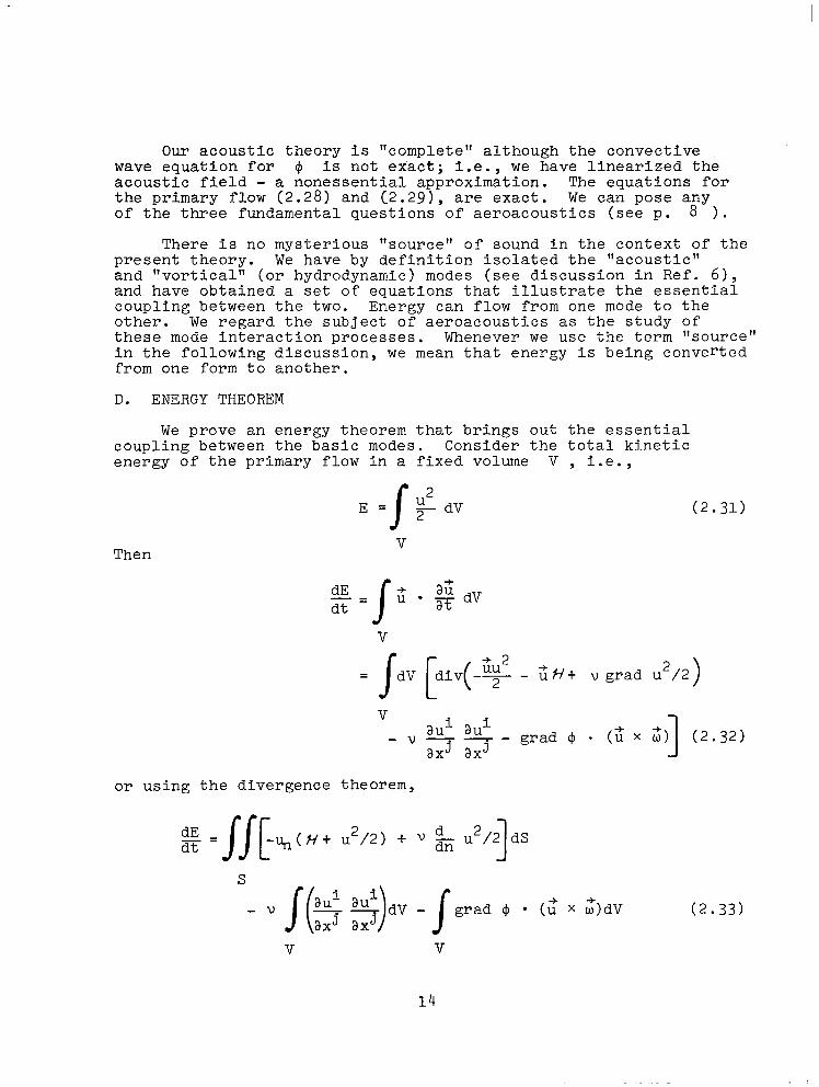
Our acoustic theory is "complete" although the convective wave equation for 4 is not exact; i.e., we have linearized the acoustic field - a nonessential approximation. The equations for the primary flow (2.28) and (2.291, are exact. We can pose any of the three fundamental questions of aeroacoustics (see p. 8 1.

There is no mysterious "source" of sound in the context of the present theory. We have by definition isolated the "acoustic" and "vertical" (or hydrodynamic) modes (see discussion in Ref. 61, and have obtained a set of equations that illustrate the essential coupling between the two. Energy can flow from one mode to the other. We regard the subject of aeroacoustics as the study of these mode interaction processes. Whenever we use the term "source" in the following discussion, we mean that energy is being converted from one form to another.

D. ENERGY THEOREM

We prove an energy theorem that brings out the essential coupling between the basic modes. Consider the total kinetic energy of the primary flow in a fixed volume V , i.e.,

(2.31)

Then

dE -= 2 l

dt i$ dV

?iH+ v grad u2/2

V -v$,ui

axJ axJ - grad $I - (c X z) 1 (2.32)

or using the divergence theorem,

dE -= dt JR

-I+#+ u2/2) + V &- u2/2 dS 1 S

- v l($ $)dV - Jgrad (p l <u' x z)dV (2.33)

V V

14

We assume that V is sufficiently large that the surface integrals in (2.33) vanish. Thus, we obtain

g = -VI (-$$)dV -Jgrad t$ l (5 x t)dV (2.34)

V V

The total kinetic energy of the primary flow can be changed by two mechanisms:

1) Viscous dissipation 2) Acoustic-vortex interaction

The conversion of kinetic energy into heat by viscous dissipation is an important physical process, but is not of direct concern to the present discussion. In fact, we cannot rigorously account for this energy since we have assumed a homentropic model of the flow. The main point of our theorem is to illustrate the importance of the Coriolis coupling term in the momentum equation and the conversion of energy from the primary flow to sound or vice versa. If the expression

grad 4 l (f x z) (2.35)

is identically zero throughout the volume V , then no acoustic energy conversion can take place. Energy conversion can only occur in those regions of the flow where there is a Coriolis acceleration 3x3 that is nonzero and .where the vorticity 0' is nonzero. It is the work done by the Coriolis force against the acoustic particle velocity that results in a local transfer of energy between modes. If the energy conversion is primarily in one direction, we can "loosely" interpret this as a production process where one mode is the "source" of the other. An important corollary to our basic theorem is that mode coupling cannot occur in regions where the primary flow has a potential. For example, energy transfer can only occur in the core regions of a vortex flow.

The energy theorem we have presented is of quite a different type than the results of Morfey (Ref. ll), who is concerned with consistent definitions of acoustic energy and fluxes that can be used to calculate noise. Our result may not be of direct computa- tional value but serves to illustrate a necessary condition for the local conversion of energy. We remark, however, that the acoustic formulation we have presented is a good starting point for the derivation of energy theorems, following the approach of Morfey.

E. THE KINETIC "ORIGIN" OF SOUND - THE LIEPMANN ANALOGY

The foregoing energy theorem has focused on the importance of vorticity for mode coupling. Without vorticity and in the absence

15

of finite boundaries, there can be no hydrodynamic flow. It is the production of vorticity by the action of viscosity at a boundary that is ultimately responsible for the unsteadiness of the primary flow and therefore of any aerodynamic sound that is produced. For the moment we shall be concerned with the question, "given a vorticity field at some instant of time, what is the mechanism whereby sound is produced in the subsequent development of the flow?" To simplify the discussion we neglect viscosity and convection in (2.27) and invoke the Lighthill hypothesis. Then,

(2.36)

Di: Dt= -grad ff + vV2G

div ?i = 0 (2.37)

The hydrodynamic flow can be calculated independent of the acoustic field (by the Lighthill hypothesis) and we have the nonlinear vorticity transport equation

RZ E =;

l grad f + vV2z

and the Poisson equation for the Bernoulli enthalpy,

(2.38)

(2.39)

From a given initial state, the solution of (2.38) will evolve independent of the acoustics. The Bernoulli enthalpy can be calculated by integration of the momentum equation or the Poisson equation (2.39). This enthalpy field is the body force distribution or acceleration potential required to maintain continuity of the incompressible flow. It acts like a Lagrange multiplier and plays no dynamic role in the evolution of the flow. The effect of a very slight compressibility is first realized in (2.36); that is,

(2.40)

is the isentropic compressibility of the medium where l/p is the specific volume. The fluctuating hydrodynamic enthalp;,Esoduces a local unsteady volume change that is proportional to . It 1s the change of the acceleration potential or Bernoulli enthalpy following the hydrodynamic fluid element that is locally responsible for the local conversion of hydrodynamic or turbulent kinetic energy into sound. The extent to which the local "dilatation"

16

sources cancel to give an overall far field sound pattern must be found by solution of the wave equation (2.36).

To complete our description of the kinetic origin of sound, we present a physical analogy that was suggested by Liepmann (Ref. 12). Consider the pendulum shown in Fig. 2.1

Fig. 2.1. The Liepmann Pendulum - Physical Analogy of Sound Production.

If the stiffness k of the rod is infinite we can calculate the primary motion of the pendulum with given initial conditions. This primary motion is analogous to the hydrodynamic flow of our present formulation. The tension in the rod is proportional to the centripetal acceleration but plays no dynamic role in the evolution of the motion. It is a Lagrange multiplier analogous to our Ber- noulli enthalpy. If the rod is slightly elastic the changing centripetal acceleration will excite an oscillation in the rod that is analogous to the sound field of our acoustic theory. Energy is converted fromthe rotational motion of the pendulum to the elastic oscillation of the rod. The coupling is via the Coriolis acceleration. If we also include a small amount of damping in the rod, we can actually damp the motion of the pendulum by analogy with acoustic radiation energy loss.

The Liepmann analogy is one of many analogies that one can construct to illustrate a very basic physical principle. When a slightly elastic rotating body undergoes a nonuniform acceleration, there is always the possibility of converting energy of the primary motion into an internal vibrational mode. The conversion of kinetic energy of a hydrodynamic vertical flow into sound is a beautiful illustration of this principle.

17

F. HOW IS SOUND PROCESSED BY A FLUID FLOW?

The second basic question of aeroacoustics that we have posed concerns the interaction of an externally applied sound field with a primary flow. For example, if we shine sound on a vortex wake or jet, we know from observation that a scattered sound field is produced. In Section III, we consider in detail the interaction of sound with a primary vortex flow. Here we briefly discuss the problem in a more general context to bring out some of the essential features of our acoustic theory.

Consider the familiar problem of sound interaction with a two-dimensional mean parallel shear flow (see Fig. 2.2). The perturbation hydrodynamic flow can be represented by a stream function JI so that

; = h,(y) + 1 - - J ax taqJ t* 0

(2.41)

and

iii = -h;(y) - Ev2qJ (2.42)

where to Y

the prime on u. the prime on u. denotes ordinary differentiation with respect denotes ordinary differentiation with respect . .

Scattered Scattered sound sound

Fig. 2.2. Acoustic Interaction with a Mean Parallel Shear Flow

18

The perturbation equations for $I , H and Jo are

V DV29 yF

0 0

T&f = ug g a2$ + 2u:, 2 ax

-g v21$ + u; 2 + v V4$ = Llg $$ + u;v2$J

and the perturbation pressure or enthalpy is given by

p’= OQ -ottH = h’ PO -

(2.43)

(2.44)

These equations may be compared with the Lilley formulation (Ref. 4) of the same problem whereby the inviscid formsof (2.3) and (2.4) are perturbed about a parallel shear flow. We get

= 2u; g (2.45)

or the single third order equation of Lilley

a2h' C t 2u' -= 0 axay

(2. 4.6 >

(2.47)

In (2.45) and (2.46), w is the vertical component of velocity (see Fig. 2.2). If the viscous terms in (2.43) are omitted, one can recombine the results to obtain the Lilley equation (2.47).

The acoustic and perturbation vertical modes are very clearly separated in (2.43). We can discuss the interactions, that result when sound impinges on the basic shearflow. The last equation for the stream function (2.43) is the Orr-Sommerfeld equation with a right-hand side that is the curl of the Coriolis coupling (see (2.28)). For most velocity profiles uo ('Y > the Orr-Sommerfeld equation has unstable modes and we expect that the acoustic input on the right-hand side will excite these modes. In other words, sound can catalyze the process whereby mean kinetic energy is converted into turbulence. The enthalpy associated with the additional turbulence will produce more sound through the first two equations. Of course, we cannot use the linear equations to study this mechanism in detail because of the inherent exponential growth of the unstable modes.

19

Instabilities of the linear perturbation equations have precipitated some discussion over the validity of the Lilley equation. In practice, any unstable modes that may exist are simply suppressed in the construction of the Green's function of the Lilley operator (Refs. 13, 14) so that the matter is primarily one of philosophy. If the unstable hydrodynamic modes are going to be suppressed (an ad hoc procedure), we can argue that an alternative procedure would be to suppress the perturbation hydrodynamic mode altogether in (2.43); i.e., set $ = 0 and solve for $I and tl (see Section III below). From this author's point of view,

a more serious objection can be raised with regard to the Lilley model and its application to the study of acoustic interactions with a fully developed turbulent shear flow. There does not appear to be any logical way of distinguishing turbulent fluctuations in the primary flow from the coherent hydrodynamic fluctuations induced by sound except when the wavelengths and frequencies of the two are significantly different. In practice, this means that scattering theories for turbulent shear flows based on the Lilley equations are probably only valid in the compact limit.

G. HOW DOES SOUND AFFECT A FLUID FLOW?

Our third basic question, the converse of the Lighthill hypothesis, is probably the most difficult to examine theoretically. The reason is that the uncertainty in calculating a meaningful primary flow is usually greater than the effect of any incident sound field. Yet, the question has been of considerable interest to the experimentalist for many years. The stability of jets to external disturbances was discussed by Lord Rayleigh (Ref. 15). More recently, Brown (Ref. 16), Hammitt (Ref. 17), Crow (Ref. 18), Bechert and Pfizenmaier (Ref.lg),and others have systematically studied the behavior of jet flows when subjected to broad band noise and pure tones. Pure tones can amplify broadband noise, and the jet itself can be excited by its own sound field or externally applied sound. These observations indicate that sound is not always a weak by-product of a primary flow as the Lighthill hypothesis asserts. Significant feedback mechanisms are possible and sho'uld be isolated experimentally and studied theoretically.

In Section V, we show how a simple vortex flow can in fact be excited by sound. The basic acoustic feedback mechanism is the Coriolis acceleration term in the momentum equation (2.28). While this term may be extremely small, it can have a profound long- term effect on the primary flow.

H. COMPARISON WITH OTHER THEORIES

To conclude our theoretical development, we compare our basic equations with several of the acoustic theories that have been proposed since the original work of Lighthill. A direct comparison

20

with a single acoustic equation with "source" cannot be made for reasons discussed earlier. We have a "complete" interactive theory without any source. To provide a common basis for discussion, we adopt the Lighthill hypothesis and create a "source" model (or acoustic analogy) as we did in Section II E. Our acoustic equation is (2.36). Our "source" is the hydrodynamic pressure or Bernoulli enthalpy that satisfies the Poisson equation (2.39). Alternative,ly, it can be calculated from the solution of (2.37). Our equations are formally analogous to the dilatation model of Ribner (Ref. 31, although Ribner uses an equation for the acoustic pressure instead of the dilatation potential. Also, for low speed flows, Ribner would replace the convective derivative of H in (2.36) by simple time derivatives; i.e.,

5 a2+ 2 i aff a at2 -v4=2=

(2.48)

v2?Y= -a2uiuj axiaxj

(2.49)

with the pressure given by

P' = PO (2.50)

sound pseudosound If we differentiate (2.48) with respect to time and use (2.49) and (2.5O), we recover Lighthill's equation for p' ; i.e.,

1 2, &s- - V2p' = p, a2uiJ

axiaxj (2.51)

The formal equivalence of our equations to those of Lighthill and Ribner in the low speed limit is thus proved.

An important point must be made concerning the approximation of replacing the substantive derivative in (2.36) by the partial time derivative in (2.48). There is a sharp distinction between the substantive derivative of H and the substantive derivative of e - In an unsteady hydrodynamic flow, both terms in the convective derivative contribute equally to DH/Dt . A good example of this is the spinning vortex pair considered in Section IV. Only at very low speeds (vortex Mach number less than 0.1) where the acoustic wavelength is many, many times the vortex separation can one consider the local derivative of H to be a suitable approximation of DH/Dt in the acoustic calculation. On the other hand, refractive effects in the acoustic operator can be neglected for relatively much larger Mach numbers. The importance of this point will become more clear when we consider the detailed calculation of the sound produced by a vortex pair.

21

The development of Powell (Ref. 20) on vortex noise is related to the present work. Where we have called attention to the Coriolis coupling between the acoustic field and the primary flow Powell has developed a source theory starting with the Lighthill formulation that focuses on the Coriolis acceleration of the primary flow as the imoortant source term. We can illustrate the main points of The right-hand

Powell's theory with the Lighthill equation (2.51). side is rewritten as follows

a2uiuj

axiaxj = div g+

= div(,$) t V2 u2/2 (2.52)

& -t x ; where

The solution of (2.51) is of the form

[div(z + grad u2/2)1y,~ d$ l%q

(2.53)

where the integral is over all space and the numerator is evaluated at the retarded time

T = t - ];-$//a .

Integrate by parts in (2.53) and evaluate the far field to get

where

t pi a2 4aa~lZl at2 /

[u2/21d; (2.54)

-+

L'X = 7% l

(Z x iI) (2.55)

is the projection of the Coriolis acceleration in the direction from the source to the observer. For very low Mach numbers, Powell argues that the second term is one higher order in Mach number compared to the first term. An argument used by Hardin (Ref. 21) in an alternate development of the Powell theory is that if the region of the primary flow is compact then differences in retarded times can be neglected and

22

h2/21& = (E)" (1 + O(M)) (2.56)

where E is the total energy of the primary aqd the asterisk denotes evaluation at the retarded time t - Ixl/a . But, to lowest order E is a conserved quantity (see Section 1I.D) so that the time derivative in (2.54) eliminates the term. 'Follow- ing Hardin (Ref. 21) we expand the first term in (2.54) in a Taylor series around the common retarded time and note that the total dipole moment (force) is zero in a free flow. The final form of the Powell result is

PO X'X~ a2 p'=- -- q lZ13 at2

YiFjd;; (2.57)

The second time derivative of the moment of the local Coriolis acceleration is the dominant source of the far field in the compact limit. The Powell theory is particularly easy to implement when concentrated line vortices are the dominant source. (See work of Hardin, Ref. 22. The main point is that Powell has derived a "compact" theory. If phase variations over the "source" region (the primary flow) are significant then the arguments leading to the simple result (2.57) are not valid. In our discussion of the vortex pair (a problem originally considered by Powell) we show that phase variations do become important for surprisingly low Mach number. In such cases it appears that one cannot avoid a more detailed integration over the complete hydrodynamic primary flow.

We have discussed in previous sections the connection of our theory with Lilley (Ref. 4) and with Howe (Ref. 10). The foregoing discussion of Powell's theory also pertains to the theory of Howe in the form he uses to discuss noise production. In fact he refers to the source term in his (compact) acoustic equation as the Powell dipole and writes,

- v2pf = -p, div(z x w') U-58)

The importance of compactness in the use of Lighthill's theory was discussed by Crow (Ref. 23). In modern applications of the theory, as developed say by Ribner (Ref. 3), or Mani and Balsa (Ref. 13, 14>, it is customary to assume locally compact sources and include phase differences between the various localized source regions. For turbulence generated noise at moderate speeds, this is probably correct. If the turbulence Mach number exceeds 0.1 the local source re

7 ions themselves tend to generate less noise

than the compact M law indicates, (see Section IV). These non- compact effects should be included in high speed noise theory.

23

III. INTERACTION OF SOUND WITH STEADY VORTEX FLOWS

A. PLANE WAVE - SCATTERING BY A VORTEX WITH CORE STRUCTURE

We consider the scattering of a plane wave propagating along the x-axis from a single vortex with a radial core vorticity distribution n(r) , as shown in Fig. 3.1

ver

-t Incident

wave

plane L Vorticity

3,=ih(r)

Figure 3.1 Scattering of Plane Waves by a Vortex

The tangential velocity field is given by

V(r) = $ pQ(p)dp (3.1)

We assume that the maximum Mach number of the vortex is sufficiently small that we can neglect quadratic terms. Our basic interaction model becomes

(3.2) aL DtL

Since tl is of order (M Eq. (3.2 1. Now let

V2?-/ = div (grad 4 x T'kQ) (3.3)

> we can neglect the convection terms in

24

where

-1wt @ = Re(Oi + bs)e (3.3)

ikx %= I @Oe (3.4)

To lowest order (the Born or first scattering approximation) the equations for the amplitude of the scattered field are

V2Gs + k2$, = - Sl

V2H = div s2 (3.6) where

2ikV a% -- % = TiF a0 (3.7)

9, = (grad 0, x c)fi

= - ~(ikS-@,, (3.8)

The first term in S &

is due primarily to the interaction of the sound with the poten ial flow "mantle" of the vortex while S2 is the direct Coriolis interaction with the vortex core.

While we can in principle, solve for 4 and H everywhere in the flowfield, we are primarily interested in the scattered far field. Thus, we solve Eq. (3.5) in the far field to obtain

% - T 0 i H(l)@)

s e-ik’l S,($)d$ (3.9)

where

H(')(kr) _ e 0

The solution for the 77 field is

(3.10)

H($) = & I

ln1; - sl div s,dd

1 f

=- 2n

(3.11)

where we have used the divergence theorem to obtain the last result. We calculate the scattered fields due to the mantle and core as follows. Let

% = 9, + am (3.12)

25

____-_--.._..-... ..---~.

where

Substitute Eq. .integration to

4Jc =

(3.13)

(3.14)

(3.11) into Eq. (3.13) and reverse the order of obtain

k H(')(kr) e s

-1kf 0; a-G 0 ' s2dz*

-ikf,=S: -t e % d; (3.15)

Y

The last integral is easily evaluated. We get

%=-E 0 i H(1) (k+.

P e-ikf1*'~2d; (3.16)

Now substitute Eq. (3.8) and Eq. (3.4) into Eq. (3.16) and use polar coordinates to obtain

k@Y (1) -ikyCcos (0 - 0') - cos e'] % = - qy Ho (kr) sin 0 e fi(y)dy de'

(3.17)

The integration over 8' can be carried out with the substitution

8' 5 0" + 0/2

so that r"

ec = - E $PHA1) (kr) a

ynJ,(2ky sin 8/2)dy*sin 0 (3.18)

To evaluate em we introduce polar coordinates in Eq. (3.14) and substitute for $1 from Eq. (3.4). Integrate once by parts with respect to 8' and the integral becomes

-iky[cos (0 - e0 - cos 0’1 Gm = - & $yHL')(kr) k e Vdy de' (3.19)

The integral over 8' is the sFe as in Eq. (3.17). Thus, we get

'm = + $,;H;l) (kr)

I yVJl(2ky sin 8/2)dy cos e/2 (3.20)

Integrate by parts with resPecOt to Y to obtain 00

+m = $$ c$;H;~) (kr) yRJo(2ky sin 8/2)dy cot e/2 (3.21)

26

where we have used Eq. (3.1) in the differential form

& yv = ys2 (3.22)

By comparing Eq. (3.20) and Eq. (3.21) we note that the mantle scattering has been reduced to an integral over the core vorticity. This is not too surprising, since the mantle velocity field is determined uniquely by the core vorticity. The interpretation as mantle scattering rather than core scattering is important however. Observe that Eq. (3.21) is singular in the forward scattering direction indicating a strong focus. This is due to the great extent of the flowfield around a single vortex that presents a very large cross-section to plane waves. Because of this focus effect we cannot evaluate the total sound power. Also, the basic scattering theory must be regarded as invalid in the forward scattering direction. To get a better understanding of this focus effect we consider a line sound source in the next section.

We combine Eq. (3.21) and Eq. (3.18) to obtain the final result for the scattered field.

% = 2 $yHL')(kr)cos 8 cot $Sc(0) (3.23)

where

and

co

SC0 = F

f

yRJo(2ky sin e/2>dY (3.24) 0

00 m r = 21T

d Wdy (3.25)

The intensity of the scattered field normalized to the incident intensity is

IS <

ws a@s

-= -patar >

Ii r( p

a+, a@1 > at ax.

where

s = cos e cot $ - SC(e)

27

(3.26)

(3.27)

Concentrated Vortex

For a concentrated point vortex the core factor SC is unity and the angular distribution of the scattered intensity is

S2 2 e cot 28 = cos 3

For a core without mantle the same factor is

(3.28)

s2 2e = sin (3.29)

a result previously obtained by Howe (Ref. lo>, and Yates and Sandri (Ref. 5). The basic directivity pattern, Eq. (3.24), agrees with a previous result of Miiller and Matschadt (Ref. 241, and is compared qualitatively with the core alone in Fig. 3.2

/-

Core only, Eq. (3.29)

tivity 1

Figure 3.2. Qualitative Comparison of Basic Directivity with Core Scattering Only

The dipole character of the core scattering is in sharp contrast to the quadrupole pattern with strong focus in the forward direction when the mantle is included. Further discussion of the core results is given below.

The scattered intensity is proportional to the factor

28

where X is the wavelength of the incident

of the vortex. If is the characteristic acoustic length scale the vortex is essentially transparent to the incident

For xy = O(X) or greater the validity of the Born approximation may be in question unless the core compactness is such that the amplitude of the scattered field remains bounded. We consider now the effect of various core structures.

(3.30)

sound and -

(3.31)

Solid Body Rotation

If the vorticity is constant inside the core radius rc then

= 0 r > rc

and we readily calculate

(3.32)

Jl(2krc sin e/2) SC =

krC sin e/2

(krcj2 (3.33)

;IL- 2 sin2 e/2 , kr, << 1

Exponential Core

For an exponential distribution of vorticity

a=se

-r 're

e (3.34)

we calculate

29

sc = [l + (2kre)2 sin2 f3/21-3'2

;1- 6(kre)2 sin2 0/2 , kre << 1 (3.35)

Betz Core

For aircraft wing vortices, it has been shown from the theory of Betz (Ref. 25), that the vorticity is distributed according to the formula

= 0 , r > b/3 (3.36)

The core scattering factor is

For any core we note that the principle effect is to reduce the scattered intensity. Scattering in the extreme forward direction is less affected except for large values of the compactness parameters (kr,) .

To compare the relative importance of the three cores, we require that the total vortex strength and polar moment of vorticity be the same for each distribution. Then the three core lengths are in the ratio

= (1.5 , 0.5 , 4.65) (3.38)

The reduction in scattered intensity due to the core is given approximately by the first term in the asymptotic form of each formula for SC . These terms are in the following proportion

(Solid Body, Exponential, Betz)

g (1.125 , 1.5 , 2.16)

30

The solid core is the most effective scatterer while the Betz core is the least effective. In, general, if the vorticity is more distributed, the amplitude of the scattered sound field will be less than for the equivalent concentrated vortex.

The angular distributions of the scattered intensity for the three core types are compared in Figs. 3.3 a,b,c. For the exponential and Betz cores the effect is a uniform reduction of the scattered intensity. For the solid body core we note a more complicated diffraction pattern as the core compactness ratio is increased.

Solid Body Core Without Mantle

We point out that the previous calculations of Howe (Ref. lo>, and Yates and Sandri (Ref. 51, for the scattering from a finite solid body vortex core without mantle are in error. In both cases, only the scattering due to the Corlolis interaction with the core is considered. Direct refraction in the wave operator was neglected. We can use the present results to obtain the correct answer. The vorticity distribution is

R = 5 C

H(rc - r) - $ 6(rc - rg (3.40)

where f is the total vortex strength of the core neglecting the shell of vorticity at r=rc. The scattering factor for this core is

s = cos 0 cot : J2(2krc sin 0/2)

(krc12 z-8-- sin 28 , krc << 1

The pattern is that of a pure quadrupole in contrast to the dipole pattern reported earlier (see Fig. 3.2). Also the efficienT;roT2/8. the core as a scatterer is less by the compactness factor Refraction due to direct interaction with the velocity field En the core is just as important as the Coriolis interaction.

B. ACOUSTIC INTERACTION WITH DISCRETE WEAKLY INTERACTING VORTICES

The results of the previous section are useful for estimating the importance of core structure. The basic scattering pattern is singular, however, and it is difficult to use the results in a straightforward calculation of the scattered intensity. In the present section, we consider localized noninteracting (or weakly interacting) vortices in the plane and a more general sound field.

31

SOLI

D

BOD

Y C

OR

E

W ru

_’ i ,

T, .

3.32

. Ef

fect

of

so

l: ld

bo

,dyc

ore

on

inte

nsity

di

strib

utio

n of

sc

atte

red

plan

e w

aves

.

EXPO

NEN

TIAL

C

OR

E

V J IO

cI!iL

llL

2 20

Fig.

3.

3b.

Effe

ct

of

expo

nent

iai

core

on

in

tens

ity

dist

ribut

ion

of

scat

tere

d pl

ane

wav

es.

BET2

C

OR

E

Fig.

3.

3~.

Ef’fm

nt

of

3etz

co

re

on

Tn+e

nsity

di

strib

ut?o

n of

sc

atte

red

plan

e w

aves

.

Later we consider the particular case of a line source from which we obtain the general scattering Green's function. The approach in this section is somewhat different in that we adopt a Lagrange formulation of the basic interaction process.

Consider a single line vortex interacting with an arbitrary acoustic field in the plane (Fig. 3.4). The velocity field is the SUIll of two parts

Ar \

,bitrary sound

\

Figure 3.4 Interaction of an Arbitrary Sound Field with a Line Vortex

+ v = il(?i - 1) + Ga + va = grad 4

;f;G) = y $X3: Y2

where A is the Lagrange coordinate

= grad x (3.42)

of the vortex, i.e.,

and

is= v’(Xt) dt a a (3.43)

Y r =- 2lT (3.44)

35

where l' is the vortex strength. The H field is calculated in terms of the velocity potential x , i.e.,

Again, we consider only first-order interactions and neglect all terms quadratic in y . Then

(3.46)

Our acoustic equation becomes

> ;:s + 2xa; M& - V2$ = E;(Z - A). a2e a2 aZat A ( ) (3.47)

The term on the right-hand side is the dilatati-on rate produced by the acoustic acceleration of the vortex. The coupling term on the left-hand side is again due to convective refraction by the potential flow mantle. Both terms are of the same order of importance to the interaction process.

We remark, without proof, that the scattered sound field calculated with Eq. (3.47) and incident plane waves is identical to the result obtained in the previous section (see Eq. (3.2311, with the core factor set equal to unity. The calculation is straightforward and was carried out as a check on the Lagrange formulation.

The extension of Eq. (3.47) to N noninteracting vortices is immediate. We simply add up the direct interactions on the right- hand side and use the convective velocity field due to all of the vortices on the left-hand side. We get

3 N LO+2 a2 at2 a2n= &

* t<z - it,,+ - v2f$ axat

N 1 =- c a2n=l

;<; - ~n).'iz!L

L i aZat 3 n

6

(3.48)

where -ti is the Lagrange coordinate of the nth vortex, the notion of noninveracting vortices can be made more precise with Eq. (3.48). The A 's are considered to be slowly varying functions of time by comcarison with the time required for a sound wave to traverse the complete collection of vortices. For example, if we think of the aircraft vortex wake, individual vortex filaments do not move relative to each other when viewed in a coordinate plane moving with the aircraft.

C. LINE SOURCE INTERACTION WITH A LINE VORTEX

An important special case of the foregoing theory is that of a line source of sound interacting with a line vortex as shown in Fig. 3.5. For simplicity we neglect any back reaction of the vortex flow on the acoustic source. In application, the effective source impedence would have to be estimated or derived from a separate calculation.

L ine monopo le source Vortex at origin

Figure 3.5 Line Source Interaction with a Line Vortex

The results can be used to synthesize a more general scattering Green's function for multiple vortices. Also, we can use the results directly to estimate the effect of vortex wakes on engine noise.

For a simple harmonic source at "x = z. we have

-iwt

@i 0 (1) = I$~H~ (klk - frol)e (3.49)

and the equation for the scattered amplitude is

37

V2$s + k2$s = - y- 2ik "u.- + a% a2

T mantle core (3.50)

with

+ U=~iEXJ; 21T \;;I2

(3.51)

We use the general results of Section III-A, Eqs. (3.9 - 3.14) to write

% = 9, + +m (3.52)

where

C#I~ = f& HL')(kr) f

-ik$ e dj: (3.53)

9, = - bo (')(kr) e s

-ik+ -f aGi U(Y) l -

6 6 (3.54)

From Eq. (3.49)

w. 1 - =-(#y k(; - zo)

6 I;: - Zol Hil+kl;; - :,I, (3.55)

and

$"i k; -2 H~')(kx,) (3.56) I;,1

Consider the core scattering. Substitute Eq. (3.51) and Eq. (3.56) into Eq. (3.53) to get

-ik?

= - ikr 0 H(l)(kr) H(l 4a@i 0 1 )(kxo) sin 8 (3.57 >

This is the familiar dipole pattern that we obtained with plane waves (see Eq. (3.18)). The vortex core sees a local plane wave

38

whose amplitude is reduced by the distance factor H('?kx ) . We note that the second Hankel function in Eq. (3.53) ii theOcomplete function while the first function is to be replaced by its far field asymptotic form, (see Eq. (3.10).

The'calculation of the scattered sound due to the mantle is a slightly mars complicated problem than the core calculation. We use Eq. (3.54) and introduce polar coordinates. Then

a% r 1 $.-Cm- a$ 2r y2

and after integration by parts in 8'

a% ae(

we get

(3.58)

-iky cos(8 - 8') 4Jm = - $$ $yHL')(kr) & HA')(kl; - sol) de' p

(3.59) To carry out the integration we expand the Hankel function in the integrand in a partial wave series (see (Ref. 261, page 827).

where

HL')(kl? - $,I) = w ime f

23 e Gl)mGm(~,xo) (3.60)

m=-cm

Grn(~,xo) = Jm(ky)H;')(kxo) y < x0

= Jm(kxo)H;')(ky) y > x0 (3.61)

With formulas in Ref. 27, page 254, the integral in Eq. (3.59) can be evaluated in detail. The final series solution for the total scattering is summarized below

m

@S = $$ @;l) (kr) CTm(kxo)im sin me -

H:')(kxo)

m=l T +

i sin e

Mantle Core (3.62)

with

T = A H(l) + B J m mm mm (3.63)

39

m-l

Am=l-JE-J;- 2 c

J2 m , m C kx 0

02 k=l

T J; + 2 c

Jf , ml kxo (3.64) k=m+l m-l

Bm = 1 + YmJm + 2 (3.65)

where the argument of all of the Bessel functions in the definitions of T that %hi

A B iskx For m greater than kx we remark s@r;esmconverge8 rapidly and is easy to calcalate.

The important parameter that enters the point source calculations is kx . It is 2lT times the number of wavelengths between the acoustic'source and the vortex center. In general, this parameter is not small as we shall see in specific application to vortex wakes.

The foregoing results are for point vortices. We can correct for finite core structure with the results obtained in the previous section. We simply multiply Eq. (3.62) by the core factor defined by Eq. (3.24). Also, we write down the result for multiple vortex scattering:

(3.66)

SE = p n J yRn(y)Jo(2ky sin On/2)dy (3.67)

(3.68)

where q&Y) is the vorticity distribution of the nth vortex core and fn is its total strength. Also

40

cos en = (An - Bo, CR - A,) pn - Sol l 12 - InI

(3.69)

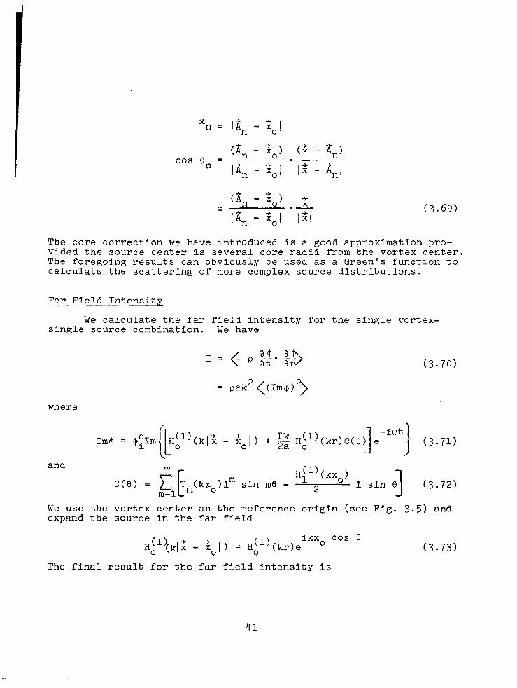
The core correction we have introduced is a good approximation pro- vided the source center is several core radii from the vortex center. The foregoing results can obviously be used as a Green's function to calculate the scattering of more complex source distributions.

Far Field Intensity

We calculate the far field intensity for the single vortex- single source combination. We have

(3.70)

= pak2<(Im$)*>

where

Im$ = 4yIm - zol) + 2 (3.71)

and 03

sin me - H;')(kxo)

2 i sin 8 1 (3.72)

We use the vortex center as the reference origin (see Fig. 3.5) and expand the source in the far field

HL')(klz - zol) = HL')(kr)e ikXo COS 8

(3.73)

The final result for the far field intensity is

41

where

I sin (kxo cos e>

+ (Re C) cos (kxo (3.74)

Ii =pa k2($o,)2

nkr (3.75)

is the source intensity. We compare the overall intensity with the source intensity in DB via the formula

'DB I

= 10 log10 q (3.76)

Note that ADB can be positive or negative. Typical results are plotted in Figs. 3.6 a,b, and c for the source location kx, = 10 and three values of the amplitude factor rk/a . Note that the back scatter is virtually zero for the smaller values of rk/a . Max- imum scattering is in the forward direction at approximately 30 degrees off the x-axis. The scattering pattern is reflected in the x- axis, if the sign of r is reversed. The strong forward scattering may be compared with the singular focus in the case of plane waves.

D. SCATTERING OF ENGINE NOISE BY AN AIRCRAFT VORTEX WAKE We now apply our vortex scattering theory to estimate the

effect of an aircraft vortex wake on engine noise. We conclude our investigation with a specific application to the DC-9 in a typical take- 9ff configuration. Strong flap vortices with r 0f 133 m /set are located approximately 5.4 m from the engine. The engine frequency at the peak Strouhal number of 0.3 is about 240 Hz. The acoustic wavelength at this frequency is about 1.5 m. The essential dimensionless parameters that we need are

kxog 25

and rkz 1.75 a

We assume that the left engine is scattered by the left wing vortex and the right engine is scattered by the right wing vortex. Also, we assume that the engine sources are incoherent so that we can superimpose the intensity in the far field. The interactive noise field for this particular configuration is shown in Fig. 3.7. We estimate that the engine noise in the aircraft ground signature is enhanced by 3 or 4 DB due to the close proximity of the flap vortices. For higher frequencies in the engine noise spectrum there could possibly be greater amplification although the vortex core structure would have to be accounted for.

42

Fig. 3.6a. Direct ivity of Intensity Relative to Unscattered Intens ity.

+I0 DB-

43

kxo = 10.0 Unscattered monopole intensity

Fig. 3.6b. I.lirect ens .ty relative to CTnsc3ttered In tensi ty.

kxo = 10.0

rkz.5 a

Unscattered Unscattered monopole intensity

Fig. 3.6~. Directivity of Intensity Relative to Unscattered Intensity.

45

Int

3 Ill3 308

Fir;. 3.7. Enp‘ir?e flap-vortex interactive noise for DC-9 in tske-off configuration.

46

These simple estimates suggest that significant variations of ground engine noise signatures can be caused by the trailing vortex configuration. If measurements are to be made of engine noise ground signatures it is recommended that a standard flap configuration be specified. These interference noise estimates could also explain discrepancies between measurements made with the same engines on different aircraft. Finally, we remark that detailed calculations of specific engine and wake configurations can be carried out with the multiple vortex scattering theory we have presented. It would be desirable, however, to develop the counterpart of Eqs. (3.66 - 3.69) for a point source near a line vortex.

In conclusion, we remark that we have focused on the weak interaction problem in the present investigation, i.e., the interaction parameter Tk/a must be of order one or less. It is equally important to consider large values of this basic parameter which means large wave numbers or high frequency. Ray acoustics theory would be the logical theory to apply. In this regard we remark that in recent work of Burnham et al (Ref. 281, results of ray theory have been used to design a wake vortex tracking system. The device works at a nominal ;y;;;es (r

f equency of 3.5 kHz so that for typical aircraft 5 = 500 m /set), the interaction parameter is of the order

. The backscatter is weak but the device works quite well at short range. It is currently operational at Kennedy airport where it is used to detect vortex decay during normal airport operation.

47

IV. PRODUCTI-ON OF SOUND BY VORTEX FLOWS

A. THE COROTATING VORTEX PAIR

We first consider an elementary two-dimensional vortex flow to which we can apply our basic acoustic formulas. The problem is that of two vortices of equal strength that spin about their centroid as shown

Fig. 4.1. Geometry of Spinning Vortex Pair

The problem has been investigated in various ways by different authors (Refs. 20,29) and is an excellent problem for comparing various aeroacoustic theories.

Source Evaluation

We use the production formulation of equations (2.36) and (2.37) with viscous effects omitted. Thus

1 a24 2 1 Dff

a2 at* -V$=z= (4.1)

Dii -= Dt - grad H (4.2)

div z = 0 (4.3)

48

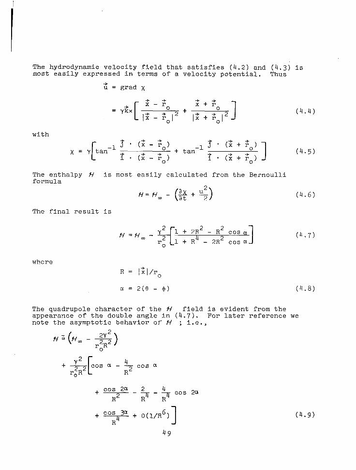
The hydrodynamic velocity field that satisfies (4.2) and (4.3) is most easily expressed in terms of a velocity potential. Thus

-t u = grad x

(4.4)

with

x = y c 3. (d-Go, tan-' -+

-& G+Go) is (;: - Go)

+tan t 1 * (Z+Go) 1 (4.5)

The enthalpy H is most easily calculated from the Bernoulli formula

H=Hm- z+p, ( The final result is

1 + 2R2 - R* cost 1 + R4 - 2R2 cos a 1

(4.6)

(4.7)

where R = l%l/ro

a = 2(9 - $I) (4.8)

The quadrupole character of the H field is evident from the appearance of the double angle in (4.7). For later reference we note the asymptotic behavior of H ; i.e.,

fjz H,-2L ( 2

r2R2 > 0

+ Y2 - cos a - r2R2 0 c

+ cos 2a - R2 2 - 3 cos 2a

+ v + 0(1/R6) R 1 (4.9)

49

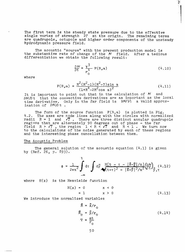
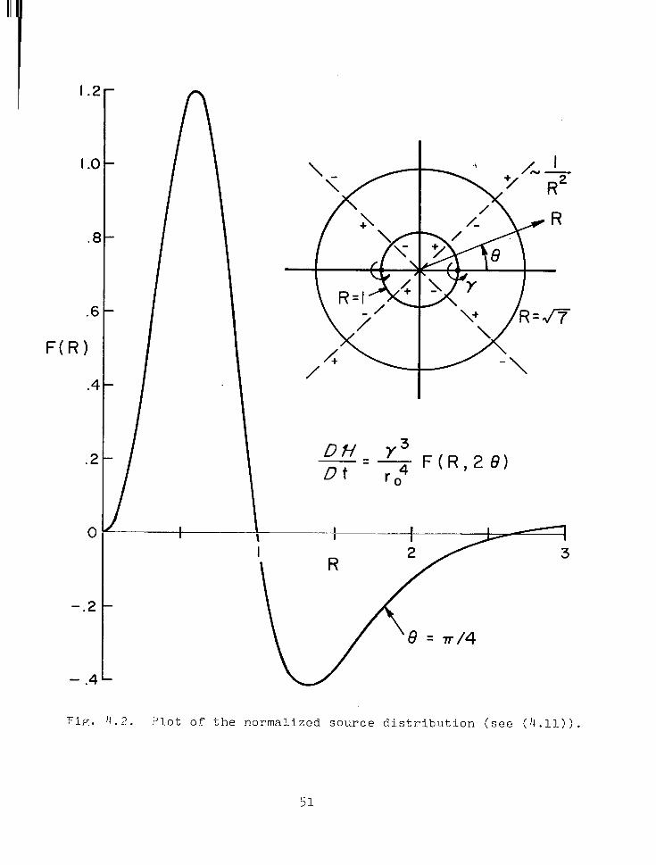
The first term is the steady state pressure due to the effective single vortex of strength 2P at the origin. The remaining terms are quadrupole, octupole and higher order components of the unsteady hydrodynamic pressure field.

The acoustic "source" with the present production model is the substantive rate of change of the H field. After a tedious differentiation we obtain the following result:

DH- Y3 ix-~ F(R,a) 0

where 2 2

F(R,a) = R (R -1)(R2-7)sin a (1+R4-2R2cos a) 2

(4.10)

(4.11)

It is important to point out that in the calculation of # and DH/D t that the convective derivatives are as important as the local time derivative. Only in the far field is aH/at a valid approximation of DffDt .

4.2. The form of the source function F(R,a) is plotted in Fig.

The axes are node lines along with the circles with normalized radii R = 1 and fl . There are three distinct annular quadrupole regions that are alternately 90 degrees out of phase - the far field R > fl , the region 1 < R < sf and R < 1 . We turn now to the calculations of the noise generated by each of these regions and the interesting phase cancellation between them.

The Acoustic Problem

The general solution of the acoustic equation (4.1) is given by (Ref. 26, p. 893).

-m

where H(x) is the Heaviside function

H(x) = 0 x < 0 = 1 x>o

We introduce the normalized variables (4.13)

rt = Z/r0

gO = S/r0 (4.14)

II I

.6

F(R)

.4

.2

0

-.2

- .4

I

DH Y3 -ET= ro4 F (R,28)

FlE. ‘1.2. plot of the normalized source distribution (see ('J-11)).

51

and the eddy Mach number Ut Slro

M=a=--c (4.15)

where .Q is the angular velocity of the spinning pair. Then

@(it,T) =

= +jd= iRodRo id@

0 0 0

H(T - I"%l) p-q-q- F[R,, 2+ - ~M(T-T)I (4.16)

The integrals in (4.16) can be evaluated if we note that F(R,a) (see (4.11)) is a periodic function of a and has a Fourier series; i.e.,

F(R,a) = n=l

S,(R) sin na (4.17)

where 7l

S,(R) = ; I

F(R,a)sin nada (4.18)

0

The coefficients S (R) can be evaluated explicitly with known results of Ref. 30,np. 113. We get

S,(R) = nR2n(7-R2) 1 + R*

, OCR<1

(4.19)

Substitute (4.17) into (4.16) and carry out the integration over T to obtain

@(z,T) = Re & .5, jn,dRord@ 0 - 0 0

s (R )e2in(+MT) n 0 Hi1)[2Mnl%ftol] (4.20)

52

We remark that the last expression could be used to evaluate 0 and all acoustic properties in the near and far field. The results could then be used to calculate refractive effects and higher order acoustic-fluid interactions. In the following, we evaluate the acoustic far field only.

For R >> 1 we have

HA1)(2mlft-301) Q H~1)(2MnR)e-2iMnRocos(e-~) (4.21)

where it is understood that the Hankel function on the right-hand side is to be replaced by its asymptotic expression (see 3.10). Substitute (4.21) into (4.20) and carry out the integration over 9 l We get

where

(4.23)

@(8,T) 2, Re * (-1)nH~1)(2MnR)e2in(e-MT)Cn (4.22) n=l 2a r 0

c, = Sn(R)J2,(2MnR)RdR

0

The total sound power radiated is given by the expression

P= -2Tr 5 & 0

-T

= 16a2(pa3ro)M7 i 4nlCn12 n=l

(4.24)

The far field solution is a series of outgoing partial waves, the leading term of which is a quadrupole whose frequency is twice the basic rotational frequency of the vortex pair. The amplitude cn of each partial wave must be evaluated numerically. The weight of the integrand in (4.23) gives us a measure of the virtual source region of the flow (see Fig. 4.2). For very small Mach number and n not too large the weight of the integrand is in the far field where R = 0(1/2Mn) . We replace Sn by its asymptotic value and obtain in the compact limit

'n Zn R-2n+lJ2n(2MnR)dR

0 n2n-1 2n-2

g 2(2n-1J M , M-t0 (4.25)

53

The first three values of Cn are as follows:

n cn 1 l/2 -I- 2 -I*/3 3 81~~180 (4.26)

The strength M3

f each higher order multipole decreases with an additional factor

From (4.24) and (4.25) we observe that in the compact limit,

P % 16a2(pa3ro)M7 (4.27)

The sound power radiated varies as M7 in accordance with known results for compact two-dimensional aeroacoustic theory (see Ref. 31). A simple M8 power law was obtained for the spinning vortex pair by Powell (Ref. 20) because he considered a segment of a three- dimensional ring pair. The M7 law was obtained by Miiller and Obermeir (Ref. 29) who solved the problem in the compact limit by matched asymptotic expansions (see below).

In the compact limit all acoustic theories seem to converge to the same answer for the acoustic power radiated. We are now in a position to place bounds on the validity of the compact limit for this simple problem. The multipole coefficients (4.23) and the sound power were evaluated numerically over a range of Mach numbers. The results are presented in Fig. 4.3. The M7 law is given by the dashed line and the numerically calculated total sound power is given by the solid line. The various multipole contributions are also shown separately for comparison purposes. The total sound power is pure quadrupole for eddy Mach numbers, less than 0.3 . The higher order poles contribute to the total sound power for higher Mach numbers although the basic calculations we have carried out are suspect for these Mach numbers. An interesting mathematical point is that the multipole series seems to diverge for M > 2/e where e is the base of the natural logarithms. Numerical calculations also indicate that this is the case.

The real significance of our calculation is for M < 0.3 . First, we observe that the compact limit is asymptotically valid for Mach numbers less than 0.1 . As the Mach number increases toward 0.3 the power radiated diminishes by 15 DB due to the noncompactness of the vortex pair structure. We remark that the acoustic wave length is 30 times the radius of the vortex pair at M = 0.1 ! This result gives an idea of how large the wave length must be to treat an eddy as compact. In a high speed turbulent flow we would expect eddy Mach numbers of the order of 0.2 to 0.3 . Our results indicate a significant reduction in the sound power due to eddy noncompactness.

54

-5

DB

-10

-15

----

w-e

--

-

-Pm

-- ----

--

-20

Tota

l

Asym

ptot

ic

quad

rupo

le

Qua

drup

ol’e

Oc

tupo

le

Hex

adec

ipol

e

-25

.I .2

.3

.4

.5

.6

.7

Eddy

M

ach

num

ber,

(~,/a

) Fi

g.

4.3

Noi

se

of

spin

ning

vo

rtex

pair

eddy

m

odel

.

Matching in the Compact Limit

A useful and familiar technique in aeroacoustics is that of matched asymptotic expansions. Crow (Ref. 23) used the technique to make a general critique of the Lighthill theory. We remarked earlier that M'iller and Obermeir (Ref. 29) used the method to solve the spinning vortex pair problem. It is a simple and powerful tool for calculating acoustic fields in the compact limit. We conclude our discussion of the vortex pair by using the idea of matching and illustrate the limitation of the method to the lowest order compact limit.

The asymptotic expansion of the hydrodynamic pressure field of the vortex pair is given by (4.9). We know that this field is transformed into an acoustic pressure field for sufficiently large R . In some intermediate overlap region the far field approximation of W should match the near field approximation of the acoustic field. We carry out the matching for the leading term in each multipole that we obtain from (4.9); i e., let

C

.2in(0-MT)

G- 1 (4.28)

The far field acoustic pressure (enthalpy) with the same phase as tl, is of the form

a4n 'n='at= Re[2inOQn(fi,T)]

= Re[2inQAnHiA)(2nMR)e2in(eBMT)] (4.29)

where A small MRn,

is to be determined by matching. We expand (4.29) for a procedure that only works if M is small. Thus

(4.30)

Now equate (4.30) and (4.28) and solve for An . We get

(4.31)

Substitute (4.31) into (4.29) and expand for large R to obtain the acoustic far field.

'n H~1)(2MnR)e2in(e-MT)Cn (4.32)

56

where

cn = n2n-1M2n-2

2(2n-l)! (4.33)

The last result is identical to (4.22) with Cn given by the compact approximation (4.25). The matching procedure yields the correct results for the multipole coefficients in the compact limit. We have not been able to obtain corrections for noncompactness via the matching procedure or any other method. It appears that a detailed integration over the near field pressure must be carried out to obtain these corrections.

B. JET IMPINGEMENT NOISE

In recent experimental work of Preisser and Block (Ref. 32) the noise of subsonic jets impinging at normal incidence on a plane wall has been carefully measured. In earlier work of Snedeker and Donaldson (Ref. 33) extensive measurements of mean flow and turbulence properties of impinging jetswere carried out. The acoustic data indicate noise levels 10 to 15 DB greater than the noise of the free jet. The flow data indicate that the turbulence levels near the impingement point are not substantially different from those in the free jet. What is the mechanism for the excessive noise? By simple imaging of the free jet sources in the plane boundary, we can argue that the noise should be 6 DB greater than the free jet. What is the origin of the other 5 to 10 DB?

From our discussion of the general problem of noise production in Section II, the physical mechanism for the impingement noise is evident. Consider a turbulent eddy (for example, the two-vortex model) that is convected along a streamline near the impingement point. The acceleration of the eddy due to streamline curvature is a real noise production mechanism. The local W-field will be magnified by the acceleration of the mean flow and so Dff/Dt will be greater. To estimate the order of the magnification, we consider the Poisson equation for W ; i.e.,

V2# = -(uV) ,i,j = i1 j’

-2iitjuJj; - u,ju,i

where we now use tensor notation and introduce a mean Ui and fluctuating velocity field ui . Recall in (2.49) and (2.51) that the source of W is the same as the source of Ribner's pseudosound equation and Lighthill's acoustic equation. The magnitude of the source of the W-field is a direct measure of the magnitude of the sound field. .We estimate the increased impingement noise by evaluating the source term, in particular the shear noise, in (4.34) for a free and impinging jet.

57

The geometry of the impingement model is shown in Fig. 4.4. We suppose that the impingement point is in the fully developed turbulent region of the free jet. The mean impingement flowfield can be well-approximated with a general result of Barnes and Sullivan (Ref. 34) who considered a Gaussian velocity profile impinging on an infinite plane wall. Unfortunately, their exact solution is a series of hypergeometric functions that converges very slowly except in the vicinity of the impingement point. There it can be shown that the mean flow can be approximated by a streamfunction that in cylindrical coordinates is of the form

I) = Cr2z (4.35)

The constant C is a measure of the curvature of the mean flow as we shall see below.

The velocity components are readily evaluated with (4.35) and we get

-1 U =li!!L=Cr

r v yj2 = 0 (4.36)

,3 = -1 w -= r ar -2cz

where is, u2 , ii3 are the contravariant components corresponding to the r 8 and z axes respectively in Fig. 4.4. of interest is'the mean shear tensor

The object

where

;i . =&+,i ¶J

ii” axJ aj (4.37)

are the nonzero Christoff& symbols for cylindrical coordinates. We substitute (4.36) and (4.38) into (4.37) to obtain the following:

ii1 aiT $1 =ar=C

yj* =r*

G2 12

ii=c

,3 = g = -2c

(4.39)

where all other components of iii . vanish. Note that the sum of the three terms in (4.39) is zerdJin accordance with the incompressible continuity equation. Also, we have introduced the physical components of the mean velocity in place of tensor components. If we substitute (4.39) into (4.34) it can easily be shown that

58

I / /-Jet ,

x Radiated

noise

wall

YM- Impingement region

Fig. 4 . II , Senmetry of Jet Implnsement Problem.

v2ff= 6c pzL + (u f'J 1) ,i,J Impinging (4.40)

4 k Jet Shear Self noise noise

Following Ribner, we call the two terms shear noise and self noise. We point out that the basic physical mechanism of the shear noise term is the "acceleration" of turbulent eddies in the curved stagnation point flow. The resulting acoustic radiation is very much analogous to the phenomenon of Brehmstrahlung radiation in atomic physics as pointed out by Williams (Ref. 35).

To bring out the essential role of the impingement acceleration we compare (4.40) with the corresponding result for a free jet where we model the mean flow as a parallel shear flow. We readily obtain

v2w= -2 & aul+ (puj’) ar az ,133

Free (4.41) Jet

The experimental results of Snedeker and Donaldson (Ref. 33) indicate that the magnitude of the turbulence is not appreciably altered by the impingement process. The turbulence is essentially frozen along streamlines until several radii from the impingement point where it re-accomodates to the wall shear. On the other hand, the experiments of Preisser and Block (Ref. 32) indicate that the acoustic source is localized within a few radii of the impingement point. Thus, we conclude that the enhancement noise must result from the shear noise term. In (4.40) the coefficient C is given by (see (4.39))

c=g (4.42)

We compare C with at/ar in (4.41). aidar

It seems plausible that for the impinging jet should be the same order of magnitude

as af/ar of the free jet. The length scale for both terms is the radius or diameter of the free jet. The velocity change in both terms must scale with the average mean flow velocity. Assuming that the two terms are the same order of magnitude, we observe that the'impingement source is greater than the free jet source by a factor of 3 . Without carrying out the detailed acoustic integrals, we can see that the factor of 3 increase in the source strength will translate into a factor of 9 in the sound power or approximately 10 DB. If this is added to the 6 DB due to imaging of the free jet, we have an estimated noise increase of 16 DB in rough agreement with the acoustic over pressure measurements of Preisser and Block.

C. A SUGGESTED PROBLEM

A detailed calculation of the radiated noise should be carried out with the source term (4.40) and measured or calculated jet

60

turbulence data. Time did not permit this calculation under the present contract. While it is important to carry out the foregoing calculation it is equally important to illuminate the physical mechanism that leads to the increased noise. A two-dimensional model problem that would illustrate the basic enhancement mechanism is the following: We have carried out a detailed calculation of the noise generated by two corotating vortices in a free flow. The next step is to imbed the pair in various accelerating mean flowfields; e.g., the stagnation point flow or mean shear flow. The noise field should be enhanced by the mean acceleration and become directional. If the eddy Mach number is sufficiently low, we can use the compact Powell theory (Ref. 20) as extended by Hardin (Ref. 21) to calculate the noise. For high speed jet impingement, we should account for noncompactness of the eddy vortex pair as shown in Section IV of this report. For the axial jet, the noise due to impinging vortex rings should be calculated. The work of Davies, et al. (Ref. 36) would again be the easiest to apply in the compact limit.

V. EXCITATION OF A FLUID FLOW BY SOUND

A. DISCUSSION OF EXPERIMENTAL RESULTS

It has long been recognized experimentally that sound can have an effect on the development of a fluid flow. For example, the transition from laminar to turbulent flow in a boundary layer can be altered at will with the incident sound field (Ref. 37). This is not surprising since the basic laminar flow is known to be sensitive to small disturbances of any kind for sufficiently large Reynolds numbers.

More interesting is the fact that turbulent flows can be stimulated or excited by impressed sound fields or by their own sound. For example, Brown (Ref. 16) has observed the excitation of jets by pure tones over a range of frequencies. He found, for example, that eddies form in the outer part of the jet at the frequency of the incident sound. For certain excitation frequencies, there was almost an explosive excitation and spreading of the jet. In other experiments, Hammitt (Ref. 17) has recorded the noise of a jet and played it back to the same jet. The result was a large amplification of the turbulence in the jet. Crow and Champagne (Ref. 18) considered the excitation of jet turbulence by upstream dis- turbance pure tones and carefully measured the enhancement of the turbulence at the excitation frequency and its harmonies. More recently, Beckert and Pfizenmaier (Ref. 19) have shown that pure tone can amplify the jet broadband noise. All of these results indicate that a free turbulent flow can be modified significantly by sound. Because of these facts, there has been a renewed interest in the excited jet as a diagnostic tool and by those who are interested in noise suppression (see Ref. 38 e.g.>.

61

If the turbulent structure of a jet could be controlled acoustically, there is the possibility of designing a more efficient noise suppressor.

B. THE LIEPMANN ANALOGY REVISITED

In Section II E, we used the Liepmann analogy to illustrate the basic mechanism of noise production by an unsteady hydrodynamic flow. With a slight extension of the analogy we can illustrate the principle of fluid excitation by sound. Suppose that we excite the vibrational mode of the Liepmann pendulum by some external source. The vibrational energy can then flow into the rotational motion of the rod. By analogy, if we shine sound on a rotating fluid element, we should be able to excite the fluid motion. In the subsequent discussion, we carry out a detailed calculation of the spinning vortex pair and show that this is indeed the case.

The following example illustrates the direct transfer of acoustic energy into the hydrodynamic vertical mode. An equally important mechanism to be considered is the catalytic effect of the sound field on the production of turbulence from the mean flow. We mentioned this point earlier in reference to acoustic stimula- tion of boundary layer transition. Also, we have seen from the linearized equations (Section II F) how the Coriolis coupling can lead to acoustic excitation of the basic instabilities of a laminar flow and, therefore, of the transition process. The analysis of transition phenomena is difficult without the complication of an acoustic field and is beyond the scope of the present study. We simply call attention to their importance and consider a more simple model problem that contains part of the basic physics.

C. EXCITATION OF THE COROTATING VORTEX PAIR

We consider two equal corotating vortices with a plane wave incident sound field as shown in Fig. 5.1. tions for the vortex centers x and B are

The Lagrangian equa-

d-A -= Y L(A-8) dt @--6I 2

+ lva sin(kz*i-wt)

dif -= y dt

iEx(&-6> + xv $-B'I 2

a sin(kzms-wt)

(5.1)

(5.2)

where v coordinaees

is the magnitude of the acoustic velocity. We introduce for the center of vorticity and the relative spacing.

&A+iB 2 ’ E = it-3 (5.31

Equation (5.1) and Eq. (5.2) become

62

.dit 1 -= .k&? dt v, sin(Zx*Lwt)cos 2

d? 2y %g + 2fv, dt= r .k&$

cos(kT=%-wt)sin 2

(5.tr)

(5.5)

The acoustically induced motion of the center of vorticity leads to scattering. We discussed this problem in detail in Section III. In the following discussion, we fix the center of vorticity and consider the acoustic effect on the relative motion. The error incurred is second order in the amplitude of the acoustic field.

We introduce the following scaling and dimensionless notation:

f = 2ro(X,Y> 2r$

, t Z-T Y

2wrg kr, Q=-=-

Y M , K = kr 0 * (5.6)

The equations for X and Y become

dX Y - = -- dT R2

+ E sin KX cos Q'r

dY X -= dT 2

where

R2 = x2 + Y2

“a

--t- incident

plane wave

(5.7)

(5.8)

Fig. 5.1. Acoustic Excitation of Vortex Pair.

63

and

E 2roVa va =- =- Y Ut

(5.9)

Y = sin T + EY' (5.10)

Then to lowest order the equations for X' , Y' are

g, - XT sin 2-c + Y' cos 2-c = sin(K cos ~)cos Pc

P1 -X’ cos 2T + Y' sin 2-c = 0 (5.11)

Two independent solutions of the homogeneous equations are

‘i = cos T + 2~ sin 'c x; = -sin T

yi = sin T - 2-r cos 'c ys = cos T (5.12)

Note that the first solution has a linear secularity; i.e., for arbitrary initial conditions the perturbation solution Will grow linearlv in time. With the homogeneous solutions (5.2), we can

is the ratio of the acoustic velocity to the orbit velocity of the vortex. An essential feature of the excitation in (5.7) is that there must be a phase difference between the velocities seen by each vortex. If the wave number K tends to zero, the incident sound looks like a hydrodynamic field to the pair and no excitation can result.

We now assume E << 1 and consider the perturbation form of (5.7). Let

x = cos T + SX'

write down the general solutions-of (5.11) in the form T X’ = (cos T + 2~ sin T) I cos t sin(rc cos

T 0

+ sin -r /

(sin t - 2t cos t)sin(lc cos t

0 T

y' = (sin T - 2-c cos T) I cos t sin(K cos

T

- cos T I 0

J 0

(sin t - 2t cos t )sin(K cos t

64

t)cos Sit dt

cos Qt dt

t)cos fit dt

(5. 13)

cos Rt dt (5.14)

where we have assumed zero initial conditions. For small K and large T it can be shown that the integrals in (5.13) and (5.14) are bounded except when Dis 2, in which case the perturbation solution grows quadratically in time; i.e.,

2 X' QJ T sin T

2 Y' % + cos T (5.15)

From the perturbation analysis, we expect that the nonlinear system will have a maximum response at the acoustic frequency corres- sponding to Sl = 2 . Note that this is also the first acoustic frequency of the vortex pair alone (see Section IV). From the scale relations (5.6) we also note that at the resonance condition

or

K = ka = HIT f = 2M

For a Mach number of order 0.1 we can have a tuned resonance condition with an acoustic wave length some 30 times the radius of the vortex pair. The resonance criteria is a frequency matching condition and does not require that the acoustic wave length match the eddy length scale.

To verify that resonance excitation of the vortex pair does occur we solved (5.7) numerically and used the results to compute the accelerations and the acoustic source UH/Dt from (4.10) and (4.11). We use the latter in the unnormalized form

DH -= ,3 r2(r2-77:) (r2-7i)sin(f3-$1

" 2 (r4-2r2r2 rO o o cos 2(8-$1 + ,:I2

(5.17)

where r vortex a8d' P

I$ are the instantaneous polar coordinates of either 0 are polar coordinates of a point in the flow-

field source rggion. The principle cause of the acoustic source is the acceleration induced by the incident acoustic field. Thus, we give a phase plot of X versus Y and a plot of Dff/Dt versus time for each case. The observation point for DH/Dt is shown in Fig. 5.2. We choose M = 0.1 and 8 = 0.06 for all cases. The magnitude of the excitation was chosen somewhat large for the purpose of visualization. The important point to observe in the following results is the relative magnitude of the response to the excitation. For reference, we first give the unexcited acoustic source in Fig. 5.2. The acceleration phase plot is a cir le (not plotted). Note the anharmonic content in the plot of DW Dt 4 . This is the source of the hfgher harmonics (see (4.26)) in the acoustic radiation of the vortex pair. In Figs. 5.3 and 5.4 we give the

65

Une

xcite

d pa

ir

M =

ut/a

=O

.I

E =

Va /

U+

=O

Fig.

5.

2.

Acou

stic

so

urce

of

an

un

exci

ted

vorte

x pa

ir,

poin

t

R=

.5

M

= 0.

1 .

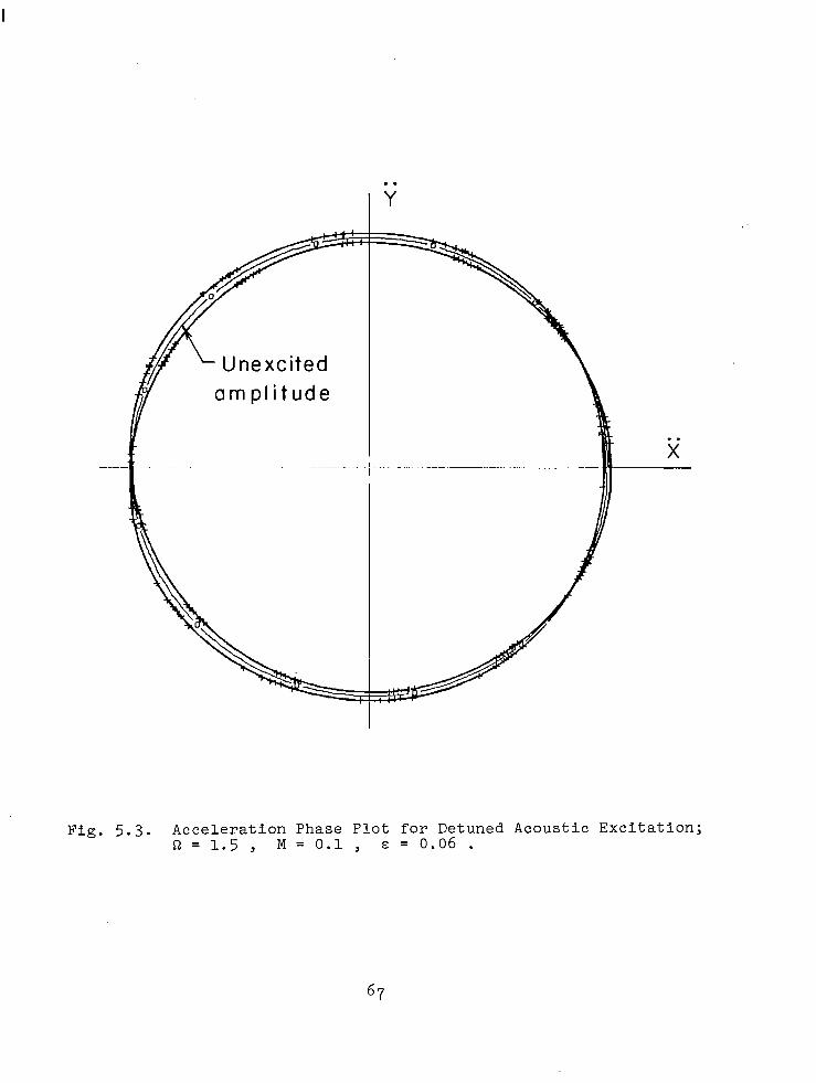
Fig. 5.3. Acceleration Phase Plot for Detuned Acoustic Excitation; L-2 = 1.5 ) M = 0.1 , E = 0.06 .

67

I

03

DH

aJ

Dt

0 -I m

/--

Une

xcite

d am

plitu

de

A P

I

I I 1

v

Fig.

5.

4.

Acou

stic

So

urce

Fu

nctio

n fo

r D

etun

ed

Acou

stic

Ex

cita

tion;

Q

= 1

.5

, M

=

0.1

, E

= -0

6 ,

R =

0.

5 .

acceleration and Dff/Dt for a highly detuned case i-2 = 1.5 . There is very little change from the unexcited case. In Figs. 5.5 and 5.6 we present the results for fi = 2. The change in DH'Dt is approximately 25 percent of the unexcited amplitude, four times the magnitude of the excitation. In Figs. 5.7, 5.8, and Figs; 5.9, 5.10, we present the results for values of R slightly more n = 2.1 and slightly less 52 = 1.9 than the linear resonance condition. In the first case, the result is much larger values of the acceleration and D#/Dt . Note that (DH/Dt) is about 50 percent greater than the unexcited case, indicating aRax amplification factor of about 8 . For s2 = 1.9 the magnitude of the acceleration and DH/Dt is attenuated by a factor of about 8 . Thus all incident acoustic frequencies in a narrow band around the fundamental pitch 52 = 2 are capable of amplifying or attenuating the basic vortex motion.

D. QUALITATIVE COMPARISON WITH EXPERIMENT

The elementary mechanism we have described for excitation of fluid motion by sound can be used to explain in part some of the experimental observations. In the experiments of Brown (Ref. 16) and Crow and Champagne (Ref. 18) pure tones were found to enhance turbulence in the frequency band near the excitation. In fact, Brown observed the formation of discrete vortices in the edge of the jet with an angular frequency equal to the excitation frequency. The jet would also become highly unstable for certain excitation frequencies. The process of vortex shedding at the nozzle lip is also excited by the incident sound and certainly plays a role in the subsequent formation of the jet. However, it seems that the complete jet can present a large cross section to the incident sound. As such, the free flow excitation mechanism we have described can be equally important.

We can use the present results to speculate on the mechanism of broadband noise amplification by pure tones that was reported by Bechert and Pfizenmaier (Ref. 19). Suppose 'that a jet flowfield is composed of "small scale" random turbulent eddies super- imposed on "large scale" coherent vortex structure. Further suppose that the random turbulent motion is acoustically more efficient than the large scale structure. Now, pure tone that is properly tuned,

if we ensonify the jet with a the vortex motion associated with

the coherent structure can be energized at the expense of the acoustic energy in the pure tone. The random turbulent flow is subsequently excited by the more energetic vortex flow and would be expected to radiate more broadband noise.

69

. . I Y

. . X

Fig. 5.5. Acceleration phase plot of acoustically excited vortex pair; R = 2.0 , M = 0.1 , E = 0.06 .

70

1

DH

Dt

4 0

P

-1

-2

f

Une

xcite

d am

plitu

de

1

Fig.

5.

6.

u

--I

Acou

stic

So

urce

Fu

nctio

n at

R

eson

ance

; R

= 2

.0

, M

= 0

.1

, E

= 0.

06

, R

= 0

.5

.

. . I Y

. . X

Fig. 5.7. Acceleration Phase Plot for Slightly Detuned Excitation; R = 2.1 , M = 0.1 , E = 0.06 .

72

z - 2 1

DN

D

! 0

-1

-'2

- \

I

t

/

Une

xcite

d am

plitu

de

J-

-

Fig.

5.

8.

Acou

stic

S

ourc

e Fu

nctio

n fo

r Sl

ight

ly

Det

uned

Ex

cita

tion;

Sl

=

2.1

, M

=

0.1

, R

=

0.5

.

Fig. 5.9. Acceleration Phase Plot for Slightly Detuned Excitation; s-2 = 1.9 , M = 0.1 , E = 0.06 .

74

-4 u-l

1

DH

Dt

0

-1

-2

I- U

nexc

ited

ampl

itude

-

Fig.

5.

10.

Acou

stic

S

ourc

e Fu

nctio

n fo

r Sl

ight

ly

Det

uned

Ex

cita

tion;

Q

=

1.9

; M

=

0.1

, E

= 0.

06

, R

=

0.5

.

VI. CONCLUSIONS

Because of the comprehensive scope of our study, we summarize our conclusions for each section separately:

A. SECTION II - ACOUSTIC THEORY

Our general theory of acoustics for hornentropic flows is self- contained and complete. We have shown that the three basic questions of aeroacoustics can be investigated systematically with the theory. The definition of sound and the concept of Bernoulli enthalpy are the fundamental building blocks. The importance of Coriolis acceleration for coupling of the acoustics and vertical modes is illuminated.

B. SECTION III - INTERACTION OF SOUND WITH VORTEX FLOWS

1. For plane wave scattering from a vortex the overall directivity is quadrupole-like with a strong focus in the forward direction. Our results are in agreement with those of Miiller and Matschadt (Ref. 24).

2. A concise formula for core scattering is derived that only involves a quadrature over the core vorticity. Vortices with distributed core vorticity (like Betz) scatter less than a more concentrated vortex.

3. The overall scatted amplitude is proportional to rk/a . Core structure is important if kr is of order 1 where rC

is the geometric extent of theCcore vorticity.

4. A general theory of acoustic scattering from discrete weakly interacting line vortices is presented. Core effects are included using the plane wave result. For a line vortex, the forward scattering focus (obtained with plane waves) is eliminated. Scattering is a maximum at about 30 degrees from the forward scattering direction. The parameter kx

e where x is the distance from the

source to the vor ex enters the scattering formula as a geometric attenuation factor.

5. The scattering theory is used to estimate the scattering of engine noise by wing vortices. For the DC-g, it is shown that scattering of jet engine frequencies near the peak Strouhal number can be of order 3 or 4 DB.

C. SECTION IV - PRODUCTION OF SOUND

1. An explicit calculation of the noise generated by a corotating vortex pair

3 s carried out. For low Mach

number (M < 0.1) the M production law is obtained in agreement with other two-dimensional compact acoustic theories.

76

2. For 0.1 < M < 0.3 it is shown that the noise is reduced by 10 to 15 DB due to noncompactness of the source region even though the radiation is basically quadrupole.

3. It is recommended that the corotating vortex pair be used to model jet impingement noise.

4. An estimate of jet impingement noise is made. We conclude that the impingement noise is due primarily to acceleration of turbulent eddies in the curved stagnation point flow. The "shear noise" source is amplified by a factor of 3 and the sound power is amplified by 'a factor of 9 or about 10 DB. The additional 6 DB due to imaging gives a total of about 15 DB. These estimates are the order of magnitude of Preisser and Block (Ref. 32).

D. SECTION V - EXCITATION OF A FLUID FLOW BY SOUND

1. It is shown that the corotating vortex pair can be excited or de-excited by an incident acoustic field. The excitation is a maximum when the incident acoustic frequency is approximately twice the rotational frequency of the pair. Amplification factors of 4 to 8 have been calculated.

2. The simple excitation model can qualitatively explain many of the experimental observations with excited jets.

77

REFERENCES

1.

2.

3.

4.

5.

6.

7.

8.

9.

10.

11.

12.

Yates, J.E., and G. Sandri, "Bernoulli Enthalpy: A Fundamental Concept in the Theory of Sound," Aeroacoustics: Jet Noise, Combustion and Core Engine Noise, Pro ress in Astronautics and Aeronautics, Vol. 43, 1976, pp. 7hT-

Lighthill, M.J., "On Sound Generated Aerodynamically, I. Gen- eral Theory," Proceedings of the Royal Society, Vol. A211, -- No. 1107, 1952, PP. 564-587, 1952.

Ribner, H.S., "The Generation of Sound by Turbulent Jets," Advances in Applied Mechanics, edited by H.L. Dryden and Th. von Karma% Academic Press, New York, 1964, pp. 103-182.

Lilley, G.M., P.J. Morris, and B.J. Tester, "On the Theory Of Jet Noise and its Applications," of Su ersonic Jet Exhaust Noise

'j?hj?h'Generation and Radiation

mAhQ=p. 3’(-41,mf ~~~~e~r~~~~,~.i~lAU~~~~~~u~f~~ and Aeronautics - Aeroacoustics: Jet and Combustion Noise; Duct -- Acoustics, Vol. 37, edited by H.T. Nagamatsu, J.V. O'Keefe, and I.R. Schwartz, AIAA, New York, pp. 3-39, 1975.

Yates, J.E., and G. Sandri, "The Role of Bernoulli Enthalpy in the Scattering of Sound," AIAA 14th Aerospace Sciences Meeting, Washington, D.C., Jan. 1976.

Chu, B., and L.S.G. Kovasznay, "Nonlinear Interactions in a Viscous Heat-Conducting Compressible Gas," Journal of Fluid Mechanics, Vol. 3, 1957-58, pp. 494-514.

--

Goldstein, M.E., "Aeroacoustics," NASA S-346, National Aero- nautics and Space Administration, 1974.

Blokhintzev, D., "The Acoustics of an Inhomogeneous Moving -- Medium, (Translationby R.T. Beyer and D. Mintzer OfRAG), Brown University, Aug. 1952.

Hinze, J.O., Turbulence, McGraw-Hill Book CO., 1959.

Howe, M.S., 'Contributions to the Theory of Aerodynamic Sound with Application to Excess Jet Noise and the Theory of the Flute," Journal of Fluid Mechanics, Vol. 71, Part 4, 1975, pp. 625-673. - -

Morfey, C.L., "Acoustic Energy in Non-uniform Flows," Sound Vib., Vol. 14, 1971, pp. 159-170.

Liepmann, H.W., lrOn the Acoustic Radiation from Boundary Layers and Jets, " Contract Report submitted to National Advisory Com- mittee for Aeronautics, Contract NAw-6288, Aug. 1954.

78

13. Mani, R., "The Influence of Jet Flow on Jet Noise, Part 1. The Noise of Unheated Jets," and "Part 2, J. Fluid Mech., Vol.

The Noise of Heated Jets," -- 73, 1976, PP. 779-793.

14. Balsa, T.F., "The Acoustic Field of Sources in Shear Flow with Application to Jet Noise: Mech.,

Convective Amplification," J. Fluid Vol. 79, 1977, PP. 33-47.

--

15. Rayleigh, J.W.S., York, 1945.

The Theory .of Sound, Dover Publication, New

16. Burniston Brown, G., IfOn Vortex Motion in Gaseous Jets and the Origin of Their Sensitivity to Sound," Phys. Sot., Vol. 47, 1935, PP. 703-732.

--

17. Hammitt, A.G., 'The Oscillation and Noise of an Overpressure Sonic Jet," J. of the Aerospace Sciences, Vol. 28, No. 9, Sept. 1961, pp.-673-680.

18. Crow, S.C., and F.H. Champagne, "Orderly Structure in Jet Turbulence," J. Fluid Mech., Vol. 48, Part 3, 1971, pp. 547- - 591.

--

19. Bechert, D., and E. Pfizenmaier, "On the Amplification of Broadband Jet Noise by a Pure Tone Excitation," Proc. of AIAA Aeroacoustics Conference, Palo Alto, Calif., July 19767 -

20. Powell, A., "Theory of Vortex Soun.d," Aerodynamic Noise, 1963, pp. 29-47.

Sept.

21. Hardin, J.C., "Noise Calculation on the Basis of Vortex Flow Models," To be presented at ASME Symposium on Noise and Fluids Engineering, Atlanta, GA, Nov. 28-30, 1977.

22. Hardin, J.C., "Analysis of Noise Produced by an Orderly Struc- ture of Turbulent Jets," NASA TN-7242, 1973.

23. Crow, S.C., "Aerodynamic Sound Emission as a Singular Perturba- tion Problem," Studies in Applied Mathematics, Vol. 49, No. 1, March 1970, pp. 21-44. -

24. Miiller, E.A., and K.R. Matschat, "The Scattering of Sound by a Single Vortex and by Turbulence," Tech. Rep. Max-Planck-Inst. ffir Stramungsforschung, Gzttingen, 1959.

25. Donaldson, C.duP., R.S. Snedeker, and R.D. Sullivan, "Calcula- tion of the Wakes of Three Transport Aircraft in Holding, Take- off, and Landing Configurations, and Comparison with Experi- mental Measurements," AFOSR-TR-73-1594 (also FAA-RD-73-421, 1973.

79

26. Morse, P.M., and H. Feshbach; Me.thdds. of The.ore't'ic'al Physics, Part I, McGraw-Hill Book Co., New Yo.rky1953.

27. Luke, Y.L., Inte rals of Bes's.el Func.tio.ns, McGraw-Hill Book Co., New York, 19 b-g--- 2.

28. Burnham, D.C., "Characteristics of a Wake-Vortex Tracking System Based on Acoustic Refractive Scattering," 2. Acoust. g. Am., Vol. 61, March 1977; also Burnham, D.C., T.E. Sullivan, and L.S. Wilk, "Measurement of Wake Vortex Strength by Means of Acoustic Back Scattering," J. Aircraft, Vol. 13, Nov. 1976, pp. 889-894.

29. MXler, E.A., and F. Obermeier, "The Spinning Vortices as a Source of Sound," Proc., Fluid Dynamics of Rotor 'and Fan Supported Aircraft at Sub- Speeds, Septm7,(AGARD). -

30. Grobner, W. and N. Hofreiter, Integraltafel Zweiter Teil Bestimmte Integrale, Wien, Springer-Verlag, 1961.

31. Ffowcs Williams, J.E., "Hydrodynamic Noise," Annual Review of Fluid Mechanics, Vol. 1, 1969, pp. 197-202.

-

32. Preisser, J-S., and P.J.W. Block, "An Experimental Study of the Aeroacoustics of a Subsonic Jet Impinging Normal to a Large Rigid Surface, " AIAA Paper 76-520. Proc. of the 3rd Aeroacous- tics Conference, Palo Alto, Calif., July 1976.

33. Snedeker, R.S., and C.duP. Donaldson, "Experiments on Free and Impinging Underexpanded Jets from a Convergent Nozzle," A.R.A.P. Report No. 63, Sept. 1964.

34. Barnes, D.A., and R.D. Sullivan, "Rotational Solutions of the Euler Equations," A.R.A.P. Report No. 79, Sept. 1965.

35. Ffowcs Williams, J.E., and M.S. Howe, "The Generation of Soundby Density Inhomogeneities in Low Mach Number Nozzle Flows," J. Fluid Mech., Vol. -- 70, 1975, PP. 605-622.

36. Davies, P.O.A.L., J.C. Hardin, A.V.J. Edwards, and J.P. Mason, "A Potential Flow Model for Calculation of Jet Noise," in Aeroacoustics: Jet Noise, Combustion and Core Engine Noise, edited by I.R. Schwartz, Vol. 43, AIAA, March m

37. Schubauer, G.B., and H.K. Skramstad, "Laminar Boundary-Layer Oscillations and Transition on a Flate Plate," NACA Rep. 909, 1948.

38. Massier, P.F., "The Role of Large Scale Turbulent Structures in Jet Noise Production," DOT/FAA Jet Noise/Core Noise Status Review, Feb. 22-24, 1977.

80

. Report No.

NASA CR-2987 . Title and Subtitla

Application of the Bernoulli Enthalpy Concept to the Study of Vortex Noise and Jet Impingement Noise.

Author(s) --

John E. Yates

Performing Organization Name and Address

Aeronautical Research Assoc. of Princeton, Inc. P.O. Box 2229 Princeton, NJ 08540

-. -__ Sponsoring Agency Name and Address

National Aeronautics and Space Administration Langley Research Center Hampton, VA 23665

Silpplementary Notes

Langley Technical Monitor: Jay C. Hardin Final Report

- 3. Recipient’s Catalog No.

----I

ii. Report Date 7

April 1978 6. Performing Organization Code

8. Performing Organizdiion Report No.

1 IO. Work Unit No.

11. Contract or Grant No.

NASl-14503

13. Type of Report and Period Covered

Contractor

14. Sponsoring Agency Code

Abstract

A complete theory of aeroacoustics of homentropic fluid medie is developed and compar with previous theories. The theory is applied to study the interaction of sound witt vortex flows, for the DC-9 in a standard take-off configuration. The maximum engine- wake interference noise is estimated to be 3 or 4 dB in the ground plane. It is shob that the noise produced by a corotating vortex pair departs significantly (10 to 15dE reductions) from the compact M scaling law for eddy Mach numbers (M) greater than 0.1. An estimate of jet impingement noise is given (-10 dB increase in sound power) that is in qualitative agreement with experimental results. The increased noise results primarily from the nonuniform acceleration of turbulent eddies through the stagnation point flow. It is shown that the corotating vortex pair can be excited or de-excited by an externally applied sound field. The model is used to quaiita- tively explain experimental results on excited jets.

Key Words [Suga?sted by Author(sl1

Aeroacoustics Bernoul 1 i Enthalpy

%curity Clawf. (of fhls r?pcrtI

Unclassified

‘. .-- .__. ~_. -- . 20. Securntv Classif. (of this pqei

18. Distribution Statement

Unclassified - Unlimited

Subject Category 71

’ For sale by the National Technical Information Service, Springfield, Virginia 22161

NASA-Langley, 1978

Application of the Bernoulli Enthalpy Concept to the … of the Bernoulli Enthalpy Concept to the...

Documents

Transcript of Application of the Bernoulli Enthalpy Concept to the … of the Bernoulli Enthalpy Concept to the...