Application of Monte Carlo methods in finance - · PDF fileStochastic processes in ﬁnance...

Stochastic processes in financeFinancial derivatives

Pricing using Monte CarloConclusions

Application of Monte Carlo methods in finance

Fred Espen Benth

Centre of Mathematics for Applications (CMA)University of Oslo, Norway

Collaborators: Lars Oswald Dahl, Martin Groth and Paul Kettler

Winter School Geilo, February 1, 2007



Overview of the lectures

1. Stochastic processes in finance

2. Financial derivativesI OptionsI Arbitrage and hedgingI Pricing of financial derivatives

3. Pricing using Monte CarloI Simulation of expectationsI Quasi-MC as variance reduction



The Bachelier modelThe Samuelson modelThe exponential NIG model

Stochastic processes in finance




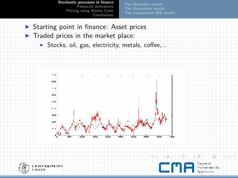
I Starting point in finance: Asset pricesI Traded prices in the market place:

I Stocks, oil, gas, electricity, metals, coffee,...




Bachelier 1900

I Future asset prices are uncertain

I Bachelier 1900: Theorie de la Speculation

I Modelled the uncertain price dynamics of stocks on the French“Bourse”

I Used probability theory to price options on stocksI Options traded on the exchange those days......

I Regnault 1853:

I The square root law for stock price variations:

S(t + s)− S(t) ∼ σ√

s




I Bachelier proposed Brownian motion with drift

S(t) = S(0) + µt + σB(t)

I Definition of Brownian motion B(t)

1. B(t + s)− B(t) is statistically independent of B(t)2. B(t + s)− B(t) is stationary, e.g., its distribution

depends only on s3. B(t + s)− B(t) is normally distributed with zero mean

and variance s.




I Property of Bachelier’s model (recall Regnault’s square rootlaw)

Var[S(t + s)− S(t)] = σ2E[(B(t + s)− B(t))2] = σ2s

I Price differences are independent and normally distributed

I Bad property: May get negative prices....




Samuelson 1965

I Samuelson: Make price dynamics positive by exponentiation

I Geometric Brownian motion (GBM)

S(t) = S(0) exp(µt + σB(t))

I What are the statistical implications of GBM?




GBM and logreturns

I Key factor in investments: The return!

S(t)− S(t − 1)

S(t − 1)

I Relative profit/loss from buying today, and selling tomorrowI Stated in percent, usually

I Key factor for the GBM model: The logreturn!

R(t) = ln

(S(t)

S(t − 1)

)= µ + σ (B(t)− B(t − 1))

I Logreturns are independent and normally distributedI Mean µI Standard deviation σ




I If the returns are small

ln

(S(t)

S(t − 1)

)≈ S(t)− S(t − 1)

S(t − 1)

I Use Taylor expansion: ln(1 + x) ≈ x

I Returns are the key in practice

I Logreturns mathematically convenient




Fitting a GBM to data

I Transform price data to logreturns

S0,S1, . . . ,Sn ⇒ R1 = ln(S1/S0), . . . ,Rn = ln(Sn/Sn−1)

I Use maximum likelihood to estimate µ and σ2 from thelogereturn data

I Example: Norsk Hydro at NYSEI Daily closing prices from Jan 1, 1990, to Dec 31, 1998I 2274 price dataI µ = 2.75%, σ = 32.8% (annualized)




I Daily closing prices of Norsk Hydro at NYSEI Two simulated GBM’s (using Monte Carlo....will come back

to this...)




I Is the normality hypothesis valid for logreturns?I Empirical distribution of NH together with fitted normal

I Note the logarithmic y-axis (frequencies)I Heavy tailsI Less probability in the center than assigned by normal




I Is the independence hypothesis valid for the logreturns?

I The autocorrelation function (ACF) for the logreturns

ρ(k) = Cov (R(t + k),R(t))

I For GBM, we find that ρ(k) = 0 theoretically

I Example where ACF for R(t),R2(t) and |R(t)| are calculatedempirically for NH

I Note that GBM should have zero ACF for all these cases




I R(t) has zero ACFI The ACF for R2(t) and |R(t)| display long range dependency

I Logreturns are not independent




A small digression

I Suppose logreturns (or returns) have non-zero correlationI Violates the market efficiency hypothesis of Samuelson (and

others)I The prices today contain all available information

I Non-zero correlation means we can predict whether returnswill be positive or negative

I Leads to possibilities to earn money riskless over timeI The traders will catch this, and speculation will rule out such

possibilities quicklyI Known as arbitrage

I The market is efficient




Alternative model for the logreturns

I Mandelbrot 70ties:I Logreturns of cotton and wool prices modelled using stable

Pareto distributions

I A recent successful model by Barndorff-Nielsen:I The normal inverse Gaussian (NIG) distributionI Used to model logreturns of stocks, currency and power pricesI ....and even temperature variations

I Original use of the NIG: Sand grain size distributionI Empirical studies on the beaches of Denmark.....I See video http://home.imf.au.dk/oebn/blownsand.mpg




I Fitting the NIG distribution to NH logreturnsI Heavy tails are explainedI Close to perfect fit in the center




The NIG distributionI 4 parameters

I µ: locationI δ: scaleI α: steepness, or tail heavinessI β: skewness

I Explicit density function

fNIG(x) = c × exp(β(x − µ))K1(α

√δ2 + (x − µ)2)√

δ2 + (x − µ)2

I K1 is the modified Bessel function of third kind and index 1 (!)

K1(x) =1

2

∫ ∞0

exp

(−1

2x(z + z−1)

)dz




I Maximum likelihood estimation of NIG for NH logreturns

α = 56, β = 2.6, µ = 0.001, δ = 0.015

I The order of estimates are typical for stock prices




Stochastic process yielding NIG logreturns?

I Let L(t) be a Levy process

1. L(t + s)− L(t) is statistically independent of L(t)2. L(t + s)− L(t) is stationary, e.g., its distribution depends

only on s

I Specify L(1) to be NIG-distributedI From property 2 we then have L(t + 1)− L(t) being NIG

I Define stochastic process for the price as

S(t) = S(0) exp(L(t))

I Exponenential NIG-Levy process




Summary so far

I 3 basic models for asset price dynamics

I Bachelier modelI Samuelson modelI exponential NIG model

I The Samuelson model is the starting point for option pricingI The theory of Black, Scholes and Merton

I Modern finance deals with incomplete marketsI The NIG model provides a typical example




Commercial break & Lottery



What are financial derivatives?The Black, Scholes and Merton theory

Financial derivatives




What are financial derivatives?

I Assets that can be traded, where the value depends onanother asset

I The standard example: Call option on stock

The owner of a call option has the right, but not theobligation, to buy one share of a stock at an agreed price and

time

I The stock is specified in the contract (e.g. NH)

I Exercise time T and strike price K likewise




I Example: Call option on Microsoft (NYSE), with exercisetime Feb 16 and K = 30

I Today’s (Jan 23) MSFT price: USD 30.74I The price of this option was USD 1.20 (Jan 23)

I Question: If you own the call option, what do you do ifI the price of MSFT is USD 32 on Feb 16?I the price of MSFT is USD 30 on Feb 16?




I Payment from call option is max(S(T )− K , 0)I The price of a call on Microsoft should be a function of the

stock priceI After all, the payment at exercise is a function of the stock

price

C (t) = f (t,S(t))?

I This is the starting point of the Black, Scholes and Mertontheory




I The option market is huge

I Put, barrier, compound, Asian options, etc.....I European and American options

I Options written on stocks, power, commodities

I Options on temperature indices

I Options on CO2 allowances




I The biggest derivatives market is the forward market

I A forward/futures contract is an agreement to trade anunderlying asset at a fixed time and price

I Example: Forward contract on electricityI Delivery of 1MWh electricity over the month of MarchI Nordpool price: 32Euro per MWhI Spot price Jan 23: 26.09 Euro per MWh

I Note that the forward price is agreed today, but paid ondelivery

I Forwards are the main traded assets in power markets

I Options are frequently written on forwards




I Forwards are (in some sense) predictions of future spot pricesI However, you pay an extra fee for the certainty

I Forward price should be a function of today’s spot price

F (t,T ) = f (t,T ,S(t))?

I Let us use the Black, Scholes and Merton theory to derive theforward price




Black, Scholes and Merton (BSM) theory

I Assume a market consisting of a spot, forward and a bank

I Spot price S(t)I Forward price denoted F (t,T )

I Delivery of spot at time T ≥ t

I Bank’s interest rate r (same for borrowing and investing)I Assume the following position: You have sold a forward

contractI The counter-party will require the spot at time TI and pay you F (t,T )

I What is your risk?I You need to provide the spot at time T !




Hedging strategy for the forward

I Buy the spot today at the price S(t)

I Finance the purchase with a loan

I Save the spot untill delivery at time T

I Receive the payment at delivery, F (t,T )I Your position at time t (today):

I Bank loan S(t) minus purchase of spot S(t) equal 0




I Your position at time T (delivery time)I You receive F (t,T ) for delivering the spotI You need to pay the loan, S(t) exp(r(T − t))

F (t,T )− S(t)er(T−t)

I If F (t,T ) > S(t)er(T−t), you have earned a riskless profit

I In a big market, you can then scale up your position, and earnan arbitrary high profit

I If F (t,T ) < S(t)er(T−t), buy forwards instead of sellingI and turn the position in the spot around

I In both cases, there are opportunities to earn a riskless profit




The no-arbitrage price

I To earn money without taking any risk is called an arbitrageI More precisely: there is arbitrageI if your position costs zero to buy,I it ends with a non-negative value,I but have a positive probability of ending strictly positive

I In any liquid market, arbitrage possibilities are ruled outquickly by competition




I Conclusion: The arbitrage-free price is

F (t,T ) = S(t)er(T−t)

I The hedging strategy is to buy spot at time t, financed by abank loan

I An investment replicating the forward completely




The forward price as an expectation

I Suppose S(t) is a GBM

I Direct calculations show

S(T ) = S(t) exp (µ(T − t) + σ(B(T )− B(t)))

E [S(T ) |S(t)] = S(t) exp((µ + 0.5σ2)(T − t)

)I The forward price has r instead of µ + 0.5σ2

I A trick from stochastic analysis: Change probability!I Everything said so far is supposing a probability space

(Ω,F ,P)




I Girsanov’s Theorem: There exists a probability Q equivalentto P such that

W (t) =µ + 0.5σ2 − r

σt + B(t)

is a Brownian motion

I Simple algebra then yields

EQ [S(T ) |S(t)] = S(t) exp(r(T − t)) = F (t,T )

I Note that the conditional expectation gives the price forgeneral processes S(t)

I First hint why MC is useful....




A little summary

I A forward is a derivative contract of the spot

I We have

1. There exists a hedging strategy, replicating the forward2. By arbitrage, we can derive the forward price from the

hedge3. There exists a probability Q such that the forward price is

expressed in terms of a conditional expectation

I These are exactly the three steps used by BSM in pricing calloptions!




Call options

I Black, Scholes and Merton developed the arbitrage theory forvaluing call options in 1972-3

I Highlight is the Black & Scholes pricing formula

I So-called “closed-form” formula for the price of call options

I Gives also the hedging strategy/replicating portfolio

I Was implemented on pocket calculators almost immediatelyafter its publication

I Publication was difficult, however!




The rise....I Scholes and Merton were awarded the Nobel Prize in

Economics in 1997

“For a new method to determine the value of derivatives”




....and fall....

I In 1998....

“Long-Term Capital Management (LTCM) was a hedge fundfounded in 1994 by John Meriwether. On its board of directorswere Myron Scholes and Robert C. Merton , who shared the1997 Nobel Memorial Prize in Economics. Initially enormouslysuccessful with annualized returns of over 40% in its firstyears, in 1998 it lost 4.6 billion USD in less than four monthsand became the most prominent example of the risk potentialin the hedge fund industry. The fund folded in early 2000.”

I Quoted from Wikipedia




The derivation of BSM

I First, some discussion of the GBM model:I Using Ito’s Formula to find the differential dS(t)

I Second-order Taylor expansion in B(t), using dB(t)2 = dt

dS(t) = µS(t) dt + σS(t) dB(t) +1

2σ2S(t) dt

I For simplicity, we write the differential as

dS(t) = αS(t) dt + σS(t) dB(t)

I May interpret dS(t) as S(t + ∆t)− S(t)




I Suppose that there exists a replicating strategy (a hedge)consisting of borrowing/investing in the bank andbuying/selling the underlying asset

V (t) = a(t)S(t) + b(t)D(t), dD(t) = rD(t) dt

I a and b are stochastic processes only depending on S(s) fors ≤ t

I V (t) is supposed to be self-financingI No witdrawal and injection of money in the hedgeI Change of positions (a, b) must come from transfer of funds

from bank to stock, or vice versa

dV (t) = a(t) dS(t) + b(t) dD(t), dD(t) = rD(t) dt




I Denote by P(t) the price, and suppose that there is a functionu(t, x) such that

P(t) = u(t,S(t))

I Applying Ito’s Formula again

dP(t) =

(ut + αuxS(t) +

1

2σ2uxxS

2(t)

)dt + σuxS(t) dB(t)

I To avoid arbitrage, V (t) = P(t)

dV (t) = (a(t)αS(t) + rb(t)D(t)) dt + σa(t)S(t) dB(t)




I Comparing the dt and dB(t) terms give

a(t) = ux(t,S(t)) , b(t) = (u(t,S(t))− a(t)S(t))/D(t)

and the PDE

ut + rxux +1

2σ2x2uxx = ru , (t, x) ∈ [0,T )× (0,∞)

I Terminal condition u(T , x) = max(x − K , 0)

I Boundary condition u(t, 0) = 0.

I Conclusion: Solve the PDE, and you have the price (andhedge)!




The Black & Scholes FormulaI Solution of the PDE: The Black & Scholes formula

P(t) = S(t)N(d1)− Ke−r(T−t)N(d2)

where

d1 =ln(S(t)/K ) + (r + 0.5σ2)(T − t)

σ√

T − t

d2 = d1 − σ√

T − t

I N(·) is the cumulative normal distribution function

N(x) = P(X ≤ x) =1√2π

∫ x

−∞e−y2/2 dy




How did they do it?????

They went down to the physics department and asked......!




A simple outline of derivation....

I Do a change of variables

v(τ, y) = eay+bτu(T − cτ, ey )

I Direct differentiation

vτ =1

2vyy , v(0, y) = eay max(ey − K , 0)

I Fundamental solution of the heat equation known to be

φ(τ, z) =1√2πτ

e−z2/2τ




I Solution v becomes

v(τ, y) =

∫ ∞−∞

eaz max(ez − K , 0)φ(τ, y − z) dz

I Transforming back to u gives the B&S formula

I Note: φ(τ, z) is the density of a Brownian motion at time τ

I Another expression of v

v(τ, y) = E[eaB(τ) max

(eB(τ) − K , 0

)|B(0) = y

]




A Feynman-Kac solution of the PDE

I Tracing backwards the expectation representation of v

u(t, x) = e−r(T−t)E[max

(S(T )− K , 0

)| S(t) = x

]where

dS(t) = r S(t) dt + σS dW (t)

I W is a Brownian motion

I Note that S is NOT S!




The option price as an expectation

I Principle in economics: The value today of a future cash flowis the discounted future cash-flow

I In language of options:

P(t) = e−r(T−t)E [max(S(T )− K , 0) |S(t)]

I A direct calculation gives P(t) 6= P(t)!

I Thus, P(t) is an arbitrage price




I Recall dynamics of S

dS(t) = αS(t) dt + σS(t) dB(t)

I Let us use Girsanov again: There exists a Q equivalent to Pso that

W (t) :=α− r

σt + B(t)

is a Brownian motionI A similar direct calculation shows

P(t) = e−r(T−t)EQ [max(S(T )− K , 0) |S(t)]




Risk-neutral probability

I Or equivalent martingale measure

I The discounted asset price S(t) is a martingale under Q

S(t) = e−r(T−t)EQ [S(T ) |S(t)]

I Using Girsanov representation, Q-dynamics is

dS(t) = rS(t) dt + σS(t) dW (t)




General derivatives pricing formula

I Suppose X is a random variable which depends on S(t) for0 ≤ t ≤ T

I X is a derivative, describing the random payment resultingfrom different scenarios of S

I Price is

P(t) = e−r(T−t)EQ [X |S(t)]




Conclusions so far...

I Price of a derivative expressible in terms of the expectedpresent value of the payoff

I The expectation with respect to QI Which in practical terms mean that α is substituted with r in

the dynamics of S(t)

I The hedge position is a(t) = ux(t,S(t))

I We are ready for some Monte Carlo



Basket optionsQuasi-Monte CarloThe exponential NIG-model

Pricing using Monte Carlo




Pricing of Basket options

I Call option written on several assets

I Examples:

I Option on a portfolioI Option on the average of several asset pricesI Spread options

I These options do not have a closed-form formula for the price




I Starting point: An d-dimensional GBM

dSi (t) = rSi (t) dt + Si (t)d∑

j=1

σij dWj(t)

I Each asset a GBMI with volatility given by (squared vol)

d∑j=1

σ2ij

I and covarianced∑

j=1

σi1jσi2j

I Dynamics directly under the risk-neutral probability Q




I Example: Option on a basket of two assetsI Exercise time T and strike price K

max (S1(T ) + S2(T )− K , 0)

I Example: Spread option

max (S1(T )− S2(T )− K , 0)

I Relevant in power marketsI For K = 0, Margrabe’s Formula

I General basket option

max

(d∑

i=1

aiSi (T )− K , 0

)




Pricing the basket

I Recall expectation operator for the price

P = e−rTEQ

[max

(d∑

i=1

aiSi (T )− K , 0

)]

I Explicit solution of Si (T ) (using Ito’s formula...)

Si (T ) = Si (0) exp

(r − 0.5d∑

j=1

σ2ij) T +

d∑j=1

σijWj(T )




I Note that in distribution

Wj(T ) =√

T Xj , Xj iid N(0, 1)

I In distribution


(r − 0.5d∑

j=1

σ2ij) T +

d∑j=1

σij

√T Xj

I Simulation of the price consists of simulation of d iid standard

normal variables Xj .




Example

I Basket of two optionsI MC vs. approximative Black & Scholes price




I Note the large variations of the price

I Time consuming to compute accurately

I In practice: Banks need prices “on-line”

I Variance-reduction is thus not for “academic fun”

I ...but crucial for the market

I One method: Quasi-Monte Carlo




Quasi-Monte Carlo

I Draw uniform numbers so that [0, 1]d gets filled optimaly

I Create a sequence of sample points u1, . . . , uN such that

DN = supB⊂[0,1]d

∣∣∣∣#un ∈ BN

− λ(B)

∣∣∣∣gets “small”

I B are boxes of the form∏d

i=1[0, ai )

I DN is the discrepancy of the sequence

I It measures the “closeness” to the uniform distribution




I A sequence is called a low discrepancy sequence if

DN ≤ C(lnN)d

N

I Many such sequences exist

I Sobol, Halton, van der Corput, de Faure etc....




Example: Halton vs. random in d = 2




Some low-discrepancy sequences

I The van der Corput sequence for d = 1 with base 2I Example of the first 16 numbers

I Sequential halfing of intervals




I Definition for a general base bI van der Corput un: Find the b-ary representation of n

n =L−1∑k=0

dk(n)bk

I Next, calculate

un =L−1∑k=0

dk(n)b−k−1

I Example: Generation of u3 with base b = 2

3 = 1× 20 + 1× 21 ,⇒ d0(3) = 1 , d1(3) = 1

u3 = 1× 2−1 + 1× 2−2 =3

4




The Halton sequence

I The Halton sequence is the d-dimensional version of the vander Corput sequence

I Choose d different bases b1, . . . , bd

I Generate un = (u1n, . . . , u

dn )

I uin generated from van der Corput with base bi

I Condition: the bases must be coprime integersI Their greates common divisor is 1




The Koksma-Hlawka bound

I Consider the integral

I =

∫[0,1]d

f (u) du

I Suppose that unNn=1 is a d-dimensional low discrepancy

sequence

IN =1

N

N∑n=1

f (un)




I The Koksma-Hlawka bound

|I − IN | ≤ Vf DN ≤ C(lnN)d

N

I Vf dependent on the variation of f




What does this have to do with finance?

I Recall the pricing expectation

P = e−rTEQ

[max

(d∑

i=1

aiSi (T )− K , 0

)]

with


(r − 0.5d∑

j=1

σ2ij) T +

d∑j=1

σij

√T Xj




I As an integral

P = e−rT

∫Rd

φ(T , x1, x2, . . . , xd)exp(−1

2

∑dj=1 x2

j )

(2π)d/2dx1 · · · dxd

I Change of variables: y = N(x)

I Recall N(x) is the cumulative standard normal distributionfunction

P = e−rT

∫[0,1]d

φ(T ,N−1(y1),N−1(y2), . . . ,N

−1(yd)) dy1 · · · dyd

I Suitable for QMC simulation




I Remark: the change of variables corresponds to

X = N−1(U)

I X normally distributed, U uniform




I Example: A basket option with two assetsI Simulation of the price using a 2D Halton sequence




The exponential NIG model

I Pricing of options when asset follows an exponential NIGmodel

I Consider a call option

P(0) = e−rTEQ

[max

(S(0)eL(T ) − K , 0

)]I L(T ) is an NIG random variable




Questions....

1. What is Q ?

2. L(T ) is NIG under P, but what is it under Q?

3. How to calculate the price ?




Question 1: Q?

I NIG-Levy process gives rise to an incomplete marketI Incomplete market:

I Option can not be replicated

I Theory of B&S: the option price is the price of replication

I So why is the price still an expectation operator under someQ?




I There exists a lot of super and sub-hedging strategiesI Superhedge

I Investment in underlying and bankI Self-financingI Worth more than option at exercise time

I Subhedge: less than

I Introduce

Psuper = infP |P is the price of a superhedgePsub = supP |P is the price of a subhedge




I Let P be so that

P ∈ (Psub,Psuper)

I It can be shown that P is an arbitrage-free priceI Not possible to make arbitrage if option has this price

I Further, for every P there exists a Q so that

P = e−rTEQ

[max

(S(0)eL(T ) − K , 0

)]




I But what is Q?????

I Q is a probability with two properties

1. Q is equivalent to P2. exp(−rt)S(t) has expectation S(0) (i.e. a martingale)

I There are many such Q’s

I One choice: Esscher transformation




Question 2: L under Q?

I Esscher transform: Structure preserving

I L(t) will be NIG-Levy under Q

I Radon-Nikodym derivative:

dQ

dP= exp (θL(T )− φ(θ)T )

I φ is the log-moment generating function of L(1)

I θ chosen so that exp(−rT )S(T ) has expectation S(0)




I A little calculation:

S(0) = EQ

[e−rTS(T )

]= e−rTS(0)E

[eL(T )eθL(T )

]e−φ(θ)T

= e−rTS(0)eφ(1+θ)T−φ(θ)T

I Choose θ so that

r = φ(1 + θ)− φ(θ)




I Suppose L(T ) ∼ NIG(α, β, µ, δ)

I Then, under Q given from Esscher

L(T ) ∼ NIG(α, β, µ, δ)

β = −1

2+ sgnβ

√α2(µ− r)2

δ2 + (µ− r)2− (µ− r)2

4δ2

I We need to calculate the expecation of the payoff from anexponential NIG




Question 3: Calculation of price

I We must simulate

P = e−rTE[max

(S(0)eX − K , 0

)]for X ∼ NIG(α, β, δ, µ)

I Note: removed the hat of β for notational laziness

I Do this by (quasi) Monte Carlo




MC simulation of NIG

I Algorithm:

1. Sample Z from IG(δ2, α2 − β2)2. Sample Y from N(0, 1)3. Return X = µ + βZ +

√Z Y

I The sampling of Z goes in several steps:




I Sampling of Z :

1. Sample V being the square of a N(0, 1) variable2. Define

W = ξ +ξ2V

2δ2− ξ

2δ2

√4ξδ2V + ξ2V 2

with ξ = δ/√

α2 − β2

3. Let

Z = W · 1U1<ξ/ξ+W +ξ2

W· 1U1≥ξ/ξ+W




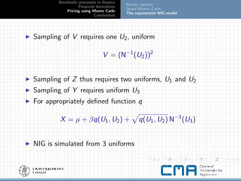
I Sampling of V requires one U2, uniform

V = (N−1(U2))2

I Sampling of Z thus requires two uniforms, U1 and U2

I Sampling of Y requires uniform U3

I For appropriately defined function q

X = µ + βq(U1,U2) +√

q(U1,U2) N−1(U3)

I NIG is simulated from 3 uniforms




I Rewriting of price expectation

P = e−rTE[max

(S(0)eX − K , 0

)]= E [f (U1,U2,U3)]

I Feasible for quasi-MC simulation




Example

I NIG parameters being “typical” for stocks

µ = 0.004 , β = −15.2 , α = 136 , δ = 0.0295

I S(0) = K = 100, r = 3.75%

I Exercise time being 1 month

I Prices simulated using MC and QMC




I Relative error as a function of number of points simulatedI “Correct” price obtained from long MC simulation



Conclusions

I Modelled financial price series with stochastic processesI BM, GBM and exponential NIG

I Priced options using arbitrage theory

I Prices are given as expectationsI Monte Carlo simulation of basket options

I GBM modelsI Using quasi-MC as variance reduction technique

I MC and exponential NIG



Not mentioned in these lectures...

I Calculations of the GreeksI Quantification of risk in portfolios

I Value-at-Risk

I Optimization of portfoliosI What is the best allocation of money....I ...given a criterion for balancing risk and return



I Valuation of swing optionsI Options where the owner has multiple rightsI Combination of control and option theory

I Real optionsI Valuation of investmentsI Example: What is the value of having the option to build a gas

pipeline to the UK?I Option theory

I All above may be solved using MC simulation



References

Black and Scholes (1973): The pricing of options and corporate liabilities. J. Political Economy, 81

Merton (1973): Theory of rational option pricing. Bell J. Econom. Managem. Sciences, 4

Samuelson (1965): Proof that properly anticipated prices fluctuate randomly. Indust. Manag. Review, 6

Davis and Etheridge (2006). Louis Bachelier’s Theory of Speculation. Princeton University Press

Dahl (2002): Numerical Analysis and Stochastic Modeling in Mathematical Finance. PhD thesis, NTNU.

Benth, Groth and Kettler (2006): A quasi-Monte Carlo algorithm for the nig distribution and valuation offinancial derivatives. Intern. J. Theoretical Applied Finance, 9.

Application of Monte Carlo methods in finance - · PDF fileStochastic processes in ﬁnance...

Documents

Transcript of Application of Monte Carlo methods in finance - · PDF fileStochastic processes in ﬁnance...