Application of Executable Architectures in Early Concept ...
129
Air Force Institute of Technology AFIT Scholar eses and Dissertations Student Graduate Works 12-24-2015 Application of Executable Architectures in Early Concept Evaluation Ryan M. Pospisal Follow this and additional works at: hps://scholar.afit.edu/etd Part of the Operations Research, Systems Engineering and Industrial Engineering Commons is esis is brought to you for free and open access by the Student Graduate Works at AFIT Scholar. It has been accepted for inclusion in eses and Dissertations by an authorized administrator of AFIT Scholar. For more information, please contact richard.mansfield@afit.edu. Recommended Citation Pospisal, Ryan M., "Application of Executable Architectures in Early Concept Evaluation" (2015). eses and Dissertations. 238. hps://scholar.afit.edu/etd/238
Transcript of Application of Executable Architectures in Early Concept ...

Air Force Institute of TechnologyAFIT Scholar
Theses and Dissertations Student Graduate Works
12-24-2015
Application of Executable Architectures in EarlyConcept EvaluationRyan M. Pospisal
Follow this and additional works at: https://scholar.afit.edu/etd
Part of the Operations Research, Systems Engineering and Industrial Engineering Commons
This Thesis is brought to you for free and open access by the Student Graduate Works at AFIT Scholar. It has been accepted for inclusion in Theses andDissertations by an authorized administrator of AFIT Scholar. For more information, please contact [email protected].
Recommended CitationPospisal, Ryan M., "Application of Executable Architectures in Early Concept Evaluation" (2015). Theses and Dissertations. 238.https://scholar.afit.edu/etd/238

APPLICATION OF EXECUTABLE ARCHITECTURES IN EARLY CONCEPT EVALUATION
THESIS
Ryan M. Pospisal, Major, USAF
AFIT-ENV-MS-15-D-027
DEPARTMENT OF THE AIR FORCE AIR UNIVERSITY
AIR FORCE INSTITUTE OF TECHNOLOGY
Wright-Patterson Air Force Base, Ohio
DISTRIBUTION STATEMENT A. APPROVED FOR PUBLIC RELEASE; DISTRIBUTION UNLIMITED.

The views expressed in this thesis are those of the author and do not reflect the official policy or position of the United States Air Force, Department of Defense, or the United States Government. This material is declared a work of the U.S. Government and is not subject to copyright protection in the United States.

AFIT-ENV-MS-15-D-027
APPLICATION OF EXECUTABLE ARCHITECTURES IN EARLY CONCEPT EVALUATION
THESIS
Presented to the Faculty
Department of Systems Engineering and Management
Graduate School of Engineering and Management
Air Force Institute of Technology
Air University
Air Education and Training Command
In Partial Fulfillment of the Requirements for the
Degree of Master of Science in Systems Engineering
Ryan M. Pospisal, B.S., Electrical Engineering
Major, USAF
December 2015
DISTRIBUTION STATEMENT A. APPROVED FOR PUBLIC RELEASE; DISTRIBUTION UNLIMITED.

AFIT-ENV-MS-15-D-027
APPLICATION OF EXECUTABLE ARCHITECTURES IN EARLY CONCEPT EVALUATION
Ryan M. Pospisal, B.S., Electrical Engineering
Major, USAF
Committee Membership:
Dr. David Jacques Chair
Dr. John Colombi Member
Lt Col Thomas Ford, PhD Member

iv
AFIT-ENV-MS-15-D-027
Abstract
This research explores use of executable architectures to guide design decisions in
the early stages of system development. Decisions made early in the system development
cycle determine a majority of the total lifecycle costs as well as establish a baseline for
long term system performance and thus it is vital to program success to choose favorable
design alternatives. The development of a representative architecture followed the
Architecture Based Evaluation Process as it provides a logical and systematic order of
events to produce an architecture sufficient to document and model operational
performance. In order to demonstrate the value in the application of executable
architectures for trade space decisions, three variants of a fictional unmanned aerial
system were developed and simulated. Four measures of effectiveness (MOEs) were
selected for evaluation. Two parameters of interest were varied at two levels during
simulation to create four test case scenarios against which to evaluate each variant.
Analysis of the resulting simulation demonstrated the ability to obtain a statistically
significant difference in MOE performance for 10 out of 16 possible test case-MOE
combinations. Additionally, for the given scenarios, the research demonstrated the ability
to make a conclusive selection of the superior variant for additional development.

v
Acknowledgments
My sincerest appreciation goes to my advisor, Dr. David Jacques, for his support, advice,
and expertise during completion of this thesis. I would also like to thank Dr. Kristen
Giammarco of the Naval Postgraduate School for advice she provided and helping secure
software licensing, without which my thesis would not have been as successful or as
interesting. Finally, I must thank my wife for her unwavering support and
encouragement throughout this process.
Ryan M. Pospisal
vi
Table of Contents
Page
Abstract .............................................................................................................................. iv
List of Figures .................................................................................................................... ix
List of Tables ..................................................................................................................... xi
1 Introduction ..................................................................................................................1
1.1 Problem Statement ..............................................................................................3
1.2 Research Objective ..............................................................................................3
1.3 Research Focus ....................................................................................................4
1.4 Methodology .......................................................................................................4
1.5 Assumptions ........................................................................................................4
1.6 Preview ................................................................................................................5
2 Literature Review .........................................................................................................7
2.1 Overview .............................................................................................................7
2.2 Definitions ...........................................................................................................7
2.3 DoDAF Background ...........................................................................................8
2.4 Simulation Techniques ......................................................................................11
2.5 Generalized Architecture Development ............................................................25
2.6 Literature Review Summary .............................................................................27
3 Methodology ..............................................................................................................28
3.1 Process ...............................................................................................................28
3.2 Assumptions ......................................................................................................28
3.3 Operational Concept ..........................................................................................29
3.4 Measures of Effectiveness .................................................................................30
vii
3.5 Architecture Scope ............................................................................................31
3.6 Required Architecture Views ............................................................................32
3.7 Development of Architecture Views .................................................................32
3.8 Development of Architecture Simulation .........................................................33
3.9 Evaluation for Model Completeness .................................................................42
3.10 Test Case Selection ........................................................................................42
3.11 Other Model Parameters ................................................................................45
3.12 Simulation Software Comments ....................................................................46
3.13 Summary ........................................................................................................48
4 Simulation Analysis and Results ................................................................................49
4.1 MOE 1: Average Target Declarations per Mission ...........................................50
4.2 MOE 2: Average Target Confirmations per Mission ........................................52
4.3 MOE 3: Average False Alarms per Mission .....................................................53
4.4 MOE 4: Average Missed Targets per Mission ..................................................57
4.5 Other Observations ............................................................................................60
4.6 Results ...............................................................................................................62
5 Conclusions and Recommendations ...........................................................................64
5.1 Recommendations for Future Research ............................................................66
Appendix A: CONOPS ......................................................................................................68
Document Overview ...................................................................................................68
Intended Users ............................................................................................................68
Document Organization..............................................................................................68
System Introduction....................................................................................................68
System Purpose ..........................................................................................................68
viii
Functional Requirements ............................................................................................69
Stakeholders ...............................................................................................................70
System Physical Description ......................................................................................71
Appendix B: AV-1 ............................................................................................................76
Architectural Description Identification .....................................................................76
Scope ..........................................................................................................................77
Purpose and Perspective .............................................................................................79
Context .......................................................................................................................79
Status ..........................................................................................................................81
Tools and File Formats ...............................................................................................81
Appendix C: OV-1: High level Operational Concept Graphic ..........................................82
Appendix D: OV-2: Operational Resource Flow Description ...........................................84
Appendix E: OV-5b: Operational Activity Model.............................................................87
Appendix F: OV-6a: Operational Rules Model .................................................................90
Appendix G: Example JavaScript ......................................................................................96
Acronyms .........................................................................................................................108
Bibliography ....................................................................................................................109

ix
List of Figures
Page
Figure 1: Flow Between Computational Models (Nakhla & Wheaton, 2014) ................. 14
Figure 2: CPN Example (Jensen, Kristesen, & Wells, 2007) ........................................... 16
Figure 3: Translation Concept from DoDAF to HCPN (Feng et al., 2010)...................... 19
Figure 4: ESSE Development Process (Cancro, Turner, Kahn, & Williams, 2011) ........ 21
Figure 5: Translation of the fUML Subset (Object Management Group, 2013) .............. 23
Figure 6: Variant 1, Partial OV-5b ................................................................................... 35
Figure 7: Variant 2, Partial OV-5b ................................................................................... 39
Figure 8: Variant 3, Partial OV-5b ................................................................................... 41
Figure 9: Average Target Declarations per Mission ......................................................... 50
Figure 10: Average Target Confirmations per Mission .................................................... 53
Figure 11: Average False Alarm Declarations per Mission.............................................. 54
Figure 12: Average False Alarm Confirmations per Mission ........................................... 56
Figure 13: Average False Alarms per Mission at System Output .................................... 57
Figure 14: Average Missed Target Declarations per Mission .......................................... 58
Figure 15: Average Missed Confirmations per Mission ................................................... 59
Figure 16: Total Average Missed Targets per Mission .................................................... 60
Figure 17: Average Evaluation Rates per Mission ........................................................... 61
Figure 18: Variant 1 and Variant 2 OV-1 ......................................................................... 82
Figure 19: Variant 3 OV-1 ................................................................................................ 83
Figure 20: Variant 1 OV-2 ................................................................................................ 84
Figure 21: Variant 2 OV-2 ................................................................................................ 85

x
Figure 22: Variant 3 OV-2 ................................................................................................ 86
Figure 23: Variant 1 OV-5b .............................................................................................. 87
Figure 24: Variant 2 OV-5b .............................................................................................. 88
Figure 25: Variant 3 OV-5b .............................................................................................. 89

xi
List of Tables
Page
Table 1: Confusion Matrix Format (with example threshold values) ............................... 37
Table 2: Confusion Matrix Logic Example ...................................................................... 37
Table 3: Test Case Matrix ................................................................................................. 43
Table 4: Sensor Low Target Detection Threshold Confusion Matrix .............................. 44
Table 5: Sensor High Target Detection Threshold Confusion Matrix .............................. 44
Table 6: Ground Control Station Confusion Matrix ......................................................... 45
Table 7: Other Model Parameters ..................................................................................... 46
Table 8: Evaluation Results Summary .............................................................................. 62
Table 9: Variant 3 JavaScript Summary ........................................................................... 96
1
APPLICATION OF EXECUTABLE ARCHITECTURES IN EARLY CONCEPT EVALUATION
1 Introduction
Procurement of state-of-the-art systems is becoming increasingly intricate and
costly as technology advancements facilitate customer requirements for increased
capabilities and extended product lifecycles. Decisions made early in system
development have an enormous impact on lifecycle costs as well as determining the
system’s performance in future use case scenarios. The use of an executable architecture
can help document, manage and guide sound decision making early in the system
development process.
Due to the increases in complexity, there is benefit to the systems engineering
(SE) community with development of executable architectures that can be used to
influence program decisions as early as possible in the acquisition lifecycle to maximize
long-term flexibility, adaptability, robustness and related “-ilities,” to ensure favorable
system and system-of-systems (SoS) performance under future uncertain applications.
The need for this toolset is further exacerbated in large SoS as total replacement becomes
cost prohibitive, thus individual systems and those comprising SoS may remain in service
for several decades and beyond.
Systems engineers and program managers must temper performance goals against
total lifecycle costs. It is estimated that conceptual and preliminary design decisions lock
in 50-75% of lifecycle costs and according to the U.S. Department of Energy, total
lifecycle cost obligation is 95% decided by the end of R&D activities (Blanchard &
Fabrycky, 2011; Makepeace, 1997). While incorporation of explicit lifecycle cost

2
estimates is beyond the scope of this thesis, it is none-the-less a practical influence that is
always under consideration.
Early trade space decisions in the acquisition process, specifically during the
Solution Analysis Phase, do not explicitly consider possible future use cases of the
system under procurement. The current version of the Defense Acquisition University's
Generic Acquisition Process, dated 17 December 2014, prescribes an Analysis of
Alternatives (AoA), but does not call for explicit consideration of future system
requirements (Defense Acquisition University, 2014). Additionally, several Department
of Defense Architecture Framework (DoDAF), Version 2.0 products, such as the
Capability Taxonomy (CV-2) and the Services Evolution Description (SvcV-8), are
mandated to address future capabilities yet the document provides little direction or
guidance on how to accomplish this requirement (DoD Deputy Chief Information
Officer, 2009).
For a given system, a deliberate decision making process that feeds into an
engineered solution accounting for other possible use cases, while minimizing resource
consumption, such as time and funding, is highly desirable. One approach to this
decision making process is to perform parametric based modeling early in program
development to indicate how a design choice affects future system performance. This
thesis explores application of an executable architecture, early in an acquisition program,
to model system performance in potential future operational scenarios and demonstrates,
via simulation, how variations of selected parameters may be used to influence system
design.

3
1.1 Problem Statement
Systems engineers and program management offices need a way of evaluating
design concepts that do not require comprehensive preliminary designs of component
systems but rather do include a number of parameters of interest across those component
systems. This evaluation supports the decision making process by informing trade
decisions during early systems acquisition. Throughout the modeling process, the
balance of time, effort, and cost inputs with the quality of model output is essential.
1.2 Research Objective
The objective of this thesis is to explore the current state of modeling methods
and tools in the SE community and implement a modest, yet representative, architecture
in an executable model using a selected toolset, with the ultimate goal of demonstrating
potential value in use of executable architectures in early concept development. To meet
these objectives, this thesis will consider the following questions:
Research Question 1: What is the capability of current architecture modeling
tools to execute simulations directly from a system architecture?
Research Question 2: What type of information can be provided from use of an
executable architecture in support of trade space decisions during early concept
development?
Research Question 3: How detailed of an executable model is required to
effectively evaluate trade space decisions in early concept modeling?
4
1.3 Research Focus
This thesis was completed under study at the Air Force’s Institute of Technology
and therefore has a Department of Defense (DoD) focus. More specifically, the research
focuses in the domain of tactical Intelligence, Surveillance, and Reconnaissance (ISR)
system development in an effort to provide a basis for application in future ISR SoS
development.
1.4 Methodology
In order to accomplish the objective, this thesis will first examine existing and
proposed methods for creating and simulating executable architectures. The author will
then comment on several commercially available architecture modeling tools to
determine their suitability for creating executable architectures and then choose a tool to
model and simulate a representative system while determining and modifying selected
model parameters to demonstrate potential value in executable architectures. Finally, an
example use of the results to guide the decision making process will be demonstrated.
1.5 Assumptions
Several broad level assumptions were identified during the research and modeling
portions of this thesis. Those assumptions are as follows:
• The concepts explored within this thesis are scalable to include more complex
individual systems and SoS.
• A commercial tool currently exists, and is accessible to the author, to document a
subset of a DoDAF V2.0 compliant system architecture and includes an
executable modeling capability to meet the fidelity requirements for this thesis.
5
• The selected sets of parameters under study are adequate to determine future
system performance.
1.6 Preview
The research and parametric modeling methods covered in this thesis are focused on DoD
centric problems however the core concepts are intended for wide application among
various commercial and governmental program management offices. Specific parameters
of interest will vary based on the system under development but the application of an
executable architecture and subsequent methods of future scenario evaluation will apply
across a range of systems.
A preview of the work by chapter is as follows:
• Chapter 1 provides an overview of the problem statement and introduction of
methodology.
• Chapter 2 is a literature review to provide a background on executable
architecture methodologies and a study of executable architecture application.
This chapter also briefly summarizes software packages featuring the various
methodologies when literature is available.
• Chapter 3 is a detailed description of application methods.
• Chapter 4 contains results and analysis of the developed executable architecture
simulations.
• Chapter 5 concludes the thesis with interpretation of the model outputs. Critical
information is the identification of parameters having the largest impact on future

6
system performance. Finally, a discussion of recommendations for future study
closes the chapter.

7
2 Literature Review
2.1 Overview
The purpose of this chapter is to provide the reader with an introduction to
executable architectures. The chapter begins by providing a baseline understanding of
architectures, architecture frameworks and their respective purposes. Following
definition, the chapter contains a review of simulation architecture techniques, discussion
of associated implementation(s), and a critique of available methods and tools.
2.2 Definitions
An executable architecture (EA) can be defined as "executable dynamic
simulations that are automatically or semi-automatically generated from architecture
models or products" (Hu, Huang, Cao, & Chang, 2014). An important characteristic of
EA over more conventional modeling and simulation (M&S) efforts is the ability to
simulate directly from existing architecture products, with minimal additional system
definition or manipulation. Use of EA in early stages of system development is helpful to
indicate system characteristics such as interoperability, capability, flexibility, and/or
maintainability and therefore to inform trade space decisions.
The Institute of Electrical and Electronics Engineers (IEEE) provides definitions
for system, design, and functional architectures. For the purposes of this thesis, the
definition of a functional architecture is the most useful and is defined as "an
arrangement of functions and their sub-functions and interfaces (internal and external)
that defines the execution sequencing, conditions for control or data flow, and the
performance requirements to satisfy the requirements baseline" (IEEE Standard 1220-
8
2005, 2007). Outputs of the functional architecture simulations are then potentially used
to influence the design architecture and thus overall system architecture.
In order to increase standardization in the system development process, the
concept of an architecture framework was created. An architectural framework serves as
a guide for constructing the various architecture products or models to thoroughly
describe and document a system. The Department of Defense (DoD) created the DoD
Architecture Framework (DoDAF) to provide a consistent modeling platform for military
system architects and engineers to describe the system under development. The DoD
describes DoDAF as:
The overarching, comprehensive framework and conceptual model enabling the
development of architectures to facilitate the ability of Department of Defense
(DoD) managers at all levels to make key decisions more effectively through
organized information sharing across the Department, Joint Capability Areas
(JCAs), Mission, Component, and Program boundaries (DoD Deputy Chief
Information Officer, 2009).
2.3 DoDAF Background
The DoD formally mandated use of an architecture framework after introduction
of the Command, Control, Communications, Computer, Intelligence, Surveillance and
Reconnaissance (C4ISR) Framework v2.0 in 1997, establishing an architecture composed
of three views; Operational, Systems and Technical. This framework was created for
information technology systems in mind and provided the system operators with an
overview of capabilities the system possessed. For the acquisition community, the

9
C4ISR framework provided a basis for determining system-of-system interoperability,
under the assumptions that the architecture accurately represented the system under study
and that none of the systems changed (Levis & Wagenhals, 2000).
In an effort to facilitate architecture use within the defense acquisition
community, the DoD introduced the DoDAF in 2003, with the intent for all system
acquisition offices to document system parameters, interactions, and dependencies via a
formal method. DoDAF differed from the previous incarnation of C4ISR by expanding
existing view definitions, introducing the All View (AV) and placed an emphasis on net-
centric concepts (Department of Defense, 2007a).
The DoD further updated the framework to DoDAF v2.0 in 2009. This new
release provided more documentation regarding information each model (formerly
referred to as products) should contain. DoD also introduced the DoDAF Meta Model
(DM2). DM2 explicitly places more emphasis on data-centric modeling. Features that
DM2 contribute to DoDAF are a constrained vocabulary, specific semantics and format,
increased discovery and understandability and finally, widely adopted integration and
analysis (DoD Deputy Chief Information Officer, 2009). Several papers cite the
ambiguous definition of terms as a significant challenge with development of executable
architectures (Ge, Hipel, Li, & Chen, 2012; Li, Dou, Ge, Yang, & Chen, 2012;
Wagenhals, Liles, & Levis, 2009). To complete the release of this updated version of the
framework, the DoDAF office provided an extensive data dictionary and mapping
resource for explicitly defining terms and mapping those terms to sub models and
products. Inclusion of this dictionary greatly improves consistency of use of terms while
developing architecture models.

10
The structure of DM2 is a data repository making it difficult to directly analyze
without first translating the data into a graphical or structured textual format (Li et al.,
2012). Under the current construct, to form an executable architecture, the data must be
extracted, comprehended, possibly modeled, and translated again into another executable
form. This not only leaves room for error but also consumes resources in the form of
money, time, and personnel.
DoDAF has proven a valuable tool in development of system architectures but it
currently only supports representation of static systems. DoDAF v1.5 identified the need
for and provided suggested methods to accomplish dynamic modeling, but those have
since been removed in newer versions of DoDAF (Department of Defense, 2007b). As
the DoD deploys more complex systems and integrates previously stand-alone systems
into SoS, the result is a continued need for dynamic representation of systems and SoS.
Successful use of an executable architecture promises to allow inclusion of
features to ensure maximum flexibility while meeting current system performance
requirements at minimum lifecycle costs. An ability to simulate possible future system
requirements and configurations plays a key role in early systems development and
selection of alternatives. By modeling foreseeable scenarios, both likely and unlikely,
and selecting system attributes based on parametric modeling, the acquisition community
can reduce lifecycle costs while increasing system flexibility, adaptability, robustness,
etc. for the user. The DoD benefits from the ability to evaluate system variations not just
in the near and mid-term, less than 5 years after system deployment, but to evaluate the
capabilities and cost for the long term, perhaps upwards of 20 years, and throughout the
product lifecycle.
11
2.4 Simulation Techniques
The modern concept of an executable architecture and application to the DoD was
first documented in a series of three companion white papers from George Mason
University in the year 2000. These techniques outlined development of a design process,
structured analysis and an object-oriented approach for the then current C4ISR
Framework (Bienvenu, Shin, & Levis, 2000; Levis & Wagenhals, 2000; Wagenhals,
Shin, Kim, & Levis, 2000). Development of executable architectures has continued to
evolve since initially conceived with realization of the efficiencies gained through direct
simulation from the architecture and increased interest from the systems engineering
community. There are still however limited mature, standardized, and user-friendly
toolsets available for creating simulations directly from an existing architecture. Along
with limited toolsets, there is no clearly preferred method for simulation of executable
architectures based on the variety of simulation techniques described in this section of the
thesis.
For the purposes of this thesis, DoDAF is considered the architecture standard of
interest, and thus defines the information required for each view. It is important to note
that while UML and SysML products are commonly used to present relevant DoDAF
views, UML and SySML do not natively include executable semantics at this time and
thus are not suitable for executable architectures (Griendling & Mavris, 2011). It is
desirable that system architecture software supports generation of all DoDAF models to
ensure concordance in addition to allowing simulations directly from those models.
Various implementations of executable architectures have been suggested and/or enacted
by academia and commercial software companies. The remainder of this chapter

12
contains a brief review of methods and various implementations proposed for EA
simulation.
2.4.1 Discrete Event Simulation
Discrete Event Simulation (DES) is a broad modeling concept without a formal
graphical notation standard. As the name implies, the simulation method divides events
into discrete periods of time to execute activities, events or processes within the model
(Griendling & Mavris, 2011). This method presents time and outputs as a step function
in the simulation rather than a linear time progression that continuous modeling
techniques offer (Matloff, 2008). DES are well suited for analyzing linear processes and
modeling discrete system changes with statistical significance (Özgün & Barlas, 2009).
Software toolkits using DES are perhaps the most commonly available and user-
friendly packages for performing system modeling and simulation with many variants
available from open source, academic and commercial producers. Examples of some of
the well-established commercial DES software packages, many including more than
exclusively DES capabilities, include Imagine That!'s Extendsim, Mathworks' SimEvent
and Rockwell Automation's Arena (Imagine That!, 2015; Mathworks, 2015; Rockwell
Automation, 2015). Unfortunately, few DES software packages, commercial or
otherwise, are purpose built for use and integration with system architectures and often
do not natively support generation of all DoDAF models. Several applications of DES
are summarized below.

13
2.4.1.1 Innoslate
SPEC Innovations has built a powerful online architecture tool called Innoslate.
This software supports generation for most of the 50 models identified in DoDAF v2.0
and allows simulation directly from some architecture models using a DES (SPEC
Innovations, 2015). Developer documentation and the author's experience were the only
sources of relevant information available for this thesis.
Benefits of the Innoslate software are many. World-wide access is provided via
the Innoslate website, allowing for platform independent architecture creation and
simulation. The built-in DES features a wide array of built-in probabilistic functions for
realistic activity durations during model execution. The software accounts for allocation
of resources and allows consumption of assigned resources throughout the simulation. In
addition to creation of the architecture models, where details can be obscured through
abstraction, the entity relationships and actions can be enhanced for simulation with
formalization through Simulation Scripts, written in simple JavaScript (SPEC
Innovations, 2015). Innoslate also includes predefined formats for many DoDAF views.
2.4.1.2 Canadian Department of National Defence
In 2014, members of the Canadian Department of National Defence's Canadian
Forces Warfare Center published a paper on a new method for creation of executable
architectures using a combination of Microsoft (MS) Visio to produce architecture
models and use of SimEvents to execute automatic simulations (Nakhla & Wheaton,
2014). Once a model is created, their method uses Visio's built-in XML generator to
export an XML file. They then process for model consistency and transform to a
SimEvents compatible file. The execution can then be run within SimEvents and updates
14
to change model behavior can be made and finally translated back to a Visio compatible
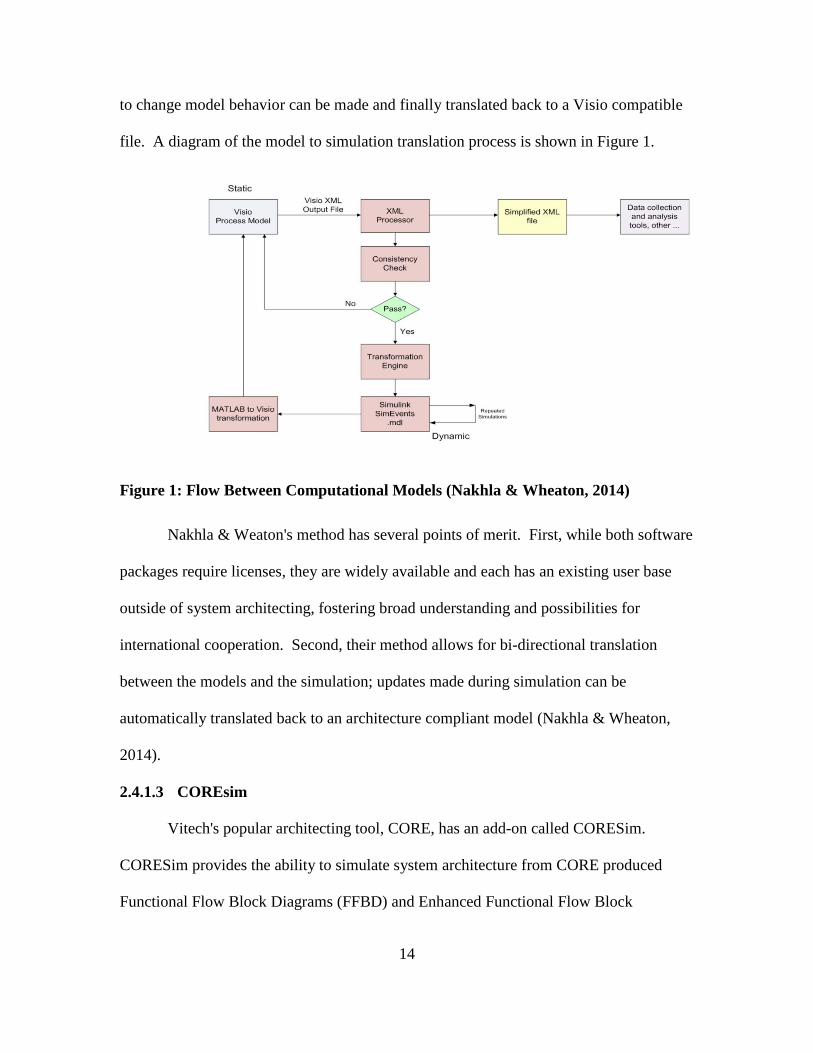
file. A diagram of the model to simulation translation process is shown in Figure 1.
Figure 1: Flow Between Computational Models (Nakhla & Wheaton, 2014)
Nakhla & Weaton's method has several points of merit. First, while both software
packages require licenses, they are widely available and each has an existing user base
outside of system architecting, fostering broad understanding and possibilities for
international cooperation. Second, their method allows for bi-directional translation
between the models and the simulation; updates made during simulation can be
automatically translated back to an architecture compliant model (Nakhla & Wheaton,
2014).
2.4.1.3 COREsim
Vitech's popular architecting tool, CORE, has an add-on called CORESim.
CORESim provides the ability to simulate system architecture from CORE produced
Functional Flow Block Diagrams (FFBD) and Enhanced Functional Flow Block

15
Diagrams (EFFBD) (Vitech Corporation, 2000). The simulator uses a DES and has a
comprehensive built-in library of probabilistic distributions available for use.
2.4.1.4 Enterprise Architect
Sparx Systems offers a comprehensive system architecting tool with built-in
simulation capabilities. The simulator uses the native UML constructs from the
architecture under simulation (Sparx Systems, 2015). The integrated simulator is useful
for discovering logical errors within the architecture but is script based and doesn't
currently allow for the addition of probabilistic variables or decision making within the
simulation. Intercax has developed a plug-in for the Enterprise Architect software to
allow execution of SysML parametric models allowing evaluation of cost, performance
and automated trade studies (Intercax, 2015b). According to the developer's published
information, the plug-in allows use of MATLAB/Simulink and Mathematica in model
development as well as export of results data for further analysis. The performance of the
plug-in was not evaluated in the completion of this thesis.
2.4.2 Colored Petri Nets
Formal notation and simulation of executable architectures though Colored Petri
Nets (CPNs) is an area of active research and is the preferred formalism for many authors
proposing executable architecture methods (Ge, Hipel, Yang, & Chen, 2014; Xia, Wu,
Liu, & Xu, 2013). CPNs are an extension of standard Petri Nets where the tokens contain
information rather than the binary token nature of standard Petri Nets. The information
contained in the tokens factor into the activation of a transition activity and thus makes it
reasonable for modeling complicated systems. CPNs retain the graphical notation of

16
Petri Nets while including consideration for data types and parameter analysis featured in
Standard Modeling Language (SML) for discrete event models (Jensen, Kristensen, &
Wells, 2007). A primary advantage of CPNs is the ability to view the model via a high
level graphic, facilitating understanding. CPNs allow transfer of attributes between
modules and sub modules, suggesting the systems can be decomposed to encourage
module reuse and improve comprehension.
A simple CPN graphic is displayed in Figure 2. Like standard Petri Nets, CPNs
contain places, transitions, and arcs, respectively represented by circles or ellipses,
rectangles and the lines connecting them. Additionally, all the above can include
annotations called inscriptions to provide detailed information. Places may contain one
or more unique inscriptions called tokens. The data at any given place is described via
these tokens.
Figure 2: CPN Example (Jensen, Kristesen, & Wells, 2007)

17
CPNs are viable for modeling executable architectures due to the ability to
include time based events. Dynamic modeling is achieved with inclusion of temporal
allocations for discrete events. Since the modules are based on discrete events,
simulations can run automatically or under direction of the architect, allowing dissection
of time and promoting a thorough understanding of system interactions (Jensen et al.,
2007).
A matter of practical interest is the complexity faced with automatic conversion of
existing architecture products or data to a CPN format through a user friendly translator.
Wagenhals et al. demonstrated a proof of concept where they developed model mapping
functions to translate widely used DoDAF product instances into an executable instance
(Wagenhals & Levis, 2009). These models would make use of existing architecture
information and products to generate an XML file capable of being read into a CPN
toolset such as CPNTools. While demonstrating the possibility of modeling this way,
Wagenhals et al. acknowledged the immaturity of this method. One problem is any
errors in the architectural instance will translate to the executable architecture and may
only be found by means of thorough examination during simulation. Once discovered,
the error must then be corrected in the initial architecture instance and translated again
into an executable form. A separate but related difficulty associated with this method is
that in some cases, the model may require double translation; once from the data to a
static model and then again from the static model to the executable model, creating
additional sources for errors (Ge et al., 2014).
Ge et al. propose a direct translation method that does not require an initial static
architecture product from which to convert to the executable model (Ge et al., 2014).
18
Their approach uses the well-defined dictionary associated with DM2 to ensure
concordance and translate directly to XML products, again to be read by a CPN toolset.
This method may reduce translation error by working through a direct translation but
rather is complicated through dependence on the rigidly defined DM2 data dictionary.
Like other methods, incorrectly entered data is not exposed until after the architecture is
simulated.
2.4.3 Hierarchical Colored Petri Nets
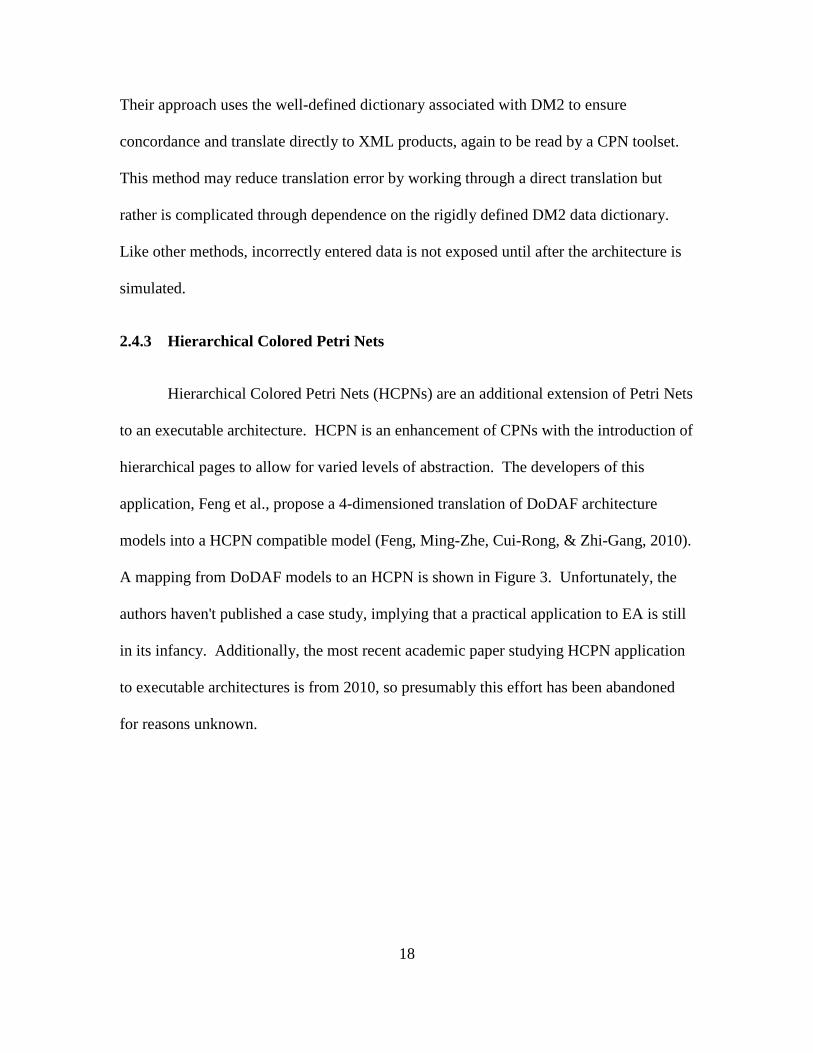
Hierarchical Colored Petri Nets (HCPNs) are an additional extension of Petri Nets
to an executable architecture. HCPN is an enhancement of CPNs with the introduction of
hierarchical pages to allow for varied levels of abstraction. The developers of this
application, Feng et al., propose a 4-dimensioned translation of DoDAF architecture
models into a HCPN compatible model (Feng, Ming-Zhe, Cui-Rong, & Zhi-Gang, 2010).
A mapping from DoDAF models to an HCPN is shown in Figure 3. Unfortunately, the
authors haven't published a case study, implying that a practical application to EA is still
in its infancy. Additionally, the most recent academic paper studying HCPN application
to executable architectures is from 2010, so presumably this effort has been abandoned
for reasons unknown.

19
Figure 3: Translation Concept from DoDAF to HCPN (Feng et al., 2010)
The overall use of CPNs or HCPNs to perform executable architectures appears to
currently be at the academic level of interest and maturity. The author of this thesis was
unable to find any formal architecture software using CPN for simulation. Several papers
suggested use of CPNs for simulation via software such as CPN Tools, but alas that
software package is not intended to be a systems architecting software and thus not
considered as a practical implementation for executable architectures (Janczura, 2009;
Jensen et al., 2007; Staines, 2008; Xia et al., 2013).
2.4.4 Executable Specification-based Systems Engineering
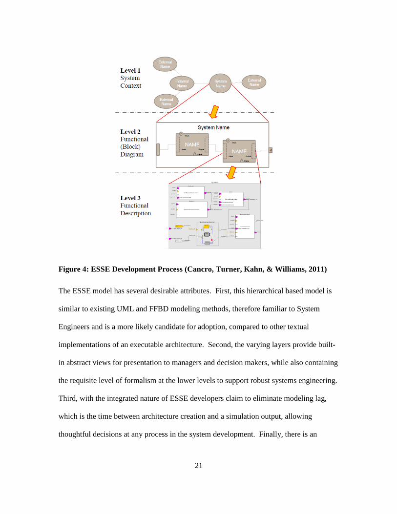
Cancro et al. describe a method for developing an executable system engineering
tool called Executable Specification-based Systems Engineering (ESSE) (Cancro, Turner,
Kahn, & Williams, 2011). The authors don't explicitly refer to this as an executable

20
architecture tool but the goals of their product, "directly executing the specification," are
consistent with the definition of an executable architecture. They propose a three level
hierarchical graphical language that specifically includes external system interaction
modeling. At the system context level, their method describes system level interactions
and is further decomposed at the second level as a Functional Block Diagram. The
implementation of functional block diagrams is especially useful in dynamic simulations
with the inclusion of flags for differentiation of clock versus interrupt driven functions
and enable flags to determine system performance in the absence of particular functions.
The third level of decomposition, termed the functional description contains highly
detailed communications interfaces (Cancro et al., 2011). A top level depiction of this
model is shown in Figure 4.
21
Figure 4: ESSE Development Process (Cancro, Turner, Kahn, & Williams, 2011)
The ESSE model has several desirable attributes. First, this hierarchical based model is
similar to existing UML and FFBD modeling methods, therefore familiar to System
Engineers and is a more likely candidate for adoption, compared to other textual
implementations of an executable architecture. Second, the varying layers provide built-
in abstract views for presentation to managers and decision makers, while also containing
the requisite level of formalism at the lower levels to support robust systems engineering.
Third, with the integrated nature of ESSE developers claim to eliminate modeling lag,
which is the time between architecture creation and a simulation output, allowing
thoughtful decisions at any process in the system development. Finally, there is an

22
apparent high level of reusability built in, a critical feature when developing a SoS.
Additionally, the developers have created a prototype development environment,
implying that it’s not ready for mass implementation (Cancro et al., 2011).
Unfortunately, the most recent publication covering this modeling concept was in 2011,
leading to an assumption that this project was abandoned for reasons unknown.
2.4.5 fUML
The Unified Modeling Language (UML) was established in 1994 as a
combination of the Booch and OMT methods of object-oriented analysis and design and
was formally released as UML 1.0 in 1997 (Larman, 2011). It has served the software
and systems engineering community well by providing a formalized language used to
develop and describe systems. One drawback of UML, current and all previous versions,
is the lack of native executable semantics to dynamically evaluate system interactions and
behaviors.
The Object Management Group (OMG), a technology standards consortium with
considerable input on the evolution of UML, recognized this gap and began developing
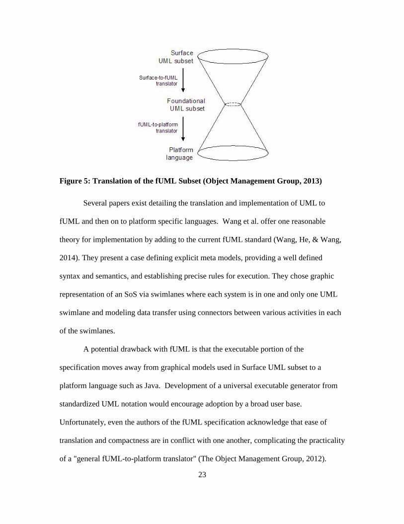
the Foundational UML (fUML). fUML is an intermediary step in the translation of
standard UML models into a platform language, such as Java. The fUML is based from
three key tenets: compactness, ease of translation and action functionality (The Object
Management Group, 2012). The fUML applies standardized language and syntax to the
translation process. A depiction of fUML’s role in translating from UML to platform
language is shown in Figure 5
23
Figure 5: Translation of the fUML Subset (Object Management Group, 2013)
Several papers exist detailing the translation and implementation of UML to
fUML and then on to platform specific languages. Wang et al. offer one reasonable
theory for implementation by adding to the current fUML standard (Wang, He, & Wang,
2014). They present a case defining explicit meta models, providing a well defined
syntax and semantics, and establishing precise rules for execution. They chose graphic
representation of an SoS via swimlanes where each system is in one and only one UML
swimlane and modeling data transfer using connectors between various activities in each
of the swimlanes.
A potential drawback with fUML is that the executable portion of the
specification moves away from graphical models used in Surface UML subset to a
platform language such as Java. Development of a universal executable generator from
standardized UML notation would encourage adoption by a broad user base.
Unfortunately, even the authors of the fUML specification acknowledge that ease of
translation and compactness are in conflict with one another, complicating the practicality
of a "general fUML-to-platform translator" (The Object Management Group, 2012).
24
Additionally, UML is an abstract modeling language and thus by defninition has poor
formalization, further comlicating direct model translation to fUML (Wang et al., 2014).
2.4.5.1 Magic Draw
Some architecture software vendors are beginning to incorporate fUML into their
execution packages. One of those examples is No Magic's MagicDraw Cameo
Simulation Toolkit which is the industry's first implementation of the fUML and State
Chart XML standards (No Magic, 2015). One criticism of this implementation is that it
lacks a global view, preventing the system engineer from viewing the complete system
and thus missing portions of the system interaction (Hu et al., 2014). No further literature
is available to outline benefits or weaknesses for this product. Similarly to Enterprise
Architect, Intercax has created a third party plug-in for Magic Draw called ParaMagic
allowing use of Mathematica, PlayerPro, OpenModelica and MATLAB for further
simulation and model analysis (Intercax, 2015a). The performance of ParaMagic was not
evaluated in the completion of this thesis.
2.4.6 Monterey Phoenix
Monterey Phoenix (MP) was initially developed for software development
applications, however similarities between software and systems acquisition provide a
favorable application to systems architecture. According to the developer, MP model
outputs are suitable for incorporation to DoDAF models however current software doesn't
support integrated architecture model generating capabilities. The benefit of MP in this
application is the ability to simulate interactions (Auguston, 2014).

25
MP defines an event as an “abstraction of activity” and is otherwise centered on
two basic premises to provide system behavior analysis; the concept of dependency in a
precedence relationship and a hierarchical relationship of inclusion (Auguston, 2014).
Auguston has formalized the executable modeling language through a syntax library.
Benefits of this model are that it provides a high level of abstraction. For
instance, an early concept evaluation isn’t dependent on strict interface control
documents and simply modeling the bulk communications between component systems
may be adequate. Another benefit is that the model simulates resource limitations and
sharing (Auguston, 2014). Like some other executable architecture programs, MP
requires unique programming and doesn't provide tailored model generation to a standard
architecture such as DoDAF. Current integrated output files and diagrams are limited to
sequence diagrams and swimlane diagrams.
2.5 Generalized Architecture Development
In addition to exploring methods of simulation, a generalized architecture
development process is appropriate for review. Dietrichs, et al. developed a set of steps
used to develop and evaluate system architectures called the Architecture Based
Evaluation Process (ABEP) (Dietrichs, Griffin, Schuettke, & Slocum, 2006). The ABEP
process identifies a logical sequence of operations for evaluation of system performance
based on simulations based on developed architecture and is not specific to development
and evaluation of an executable architecture.
Architecture Based Evaluation Process (ABEP)
ABEP ASSUMPTIONS: a. Some meaningful analysis is required to evaluate system
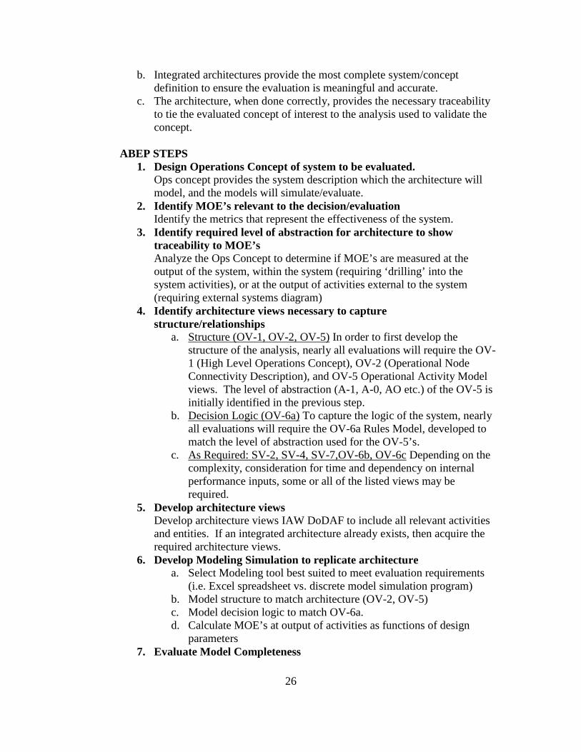
26
b. Integrated architectures provide the most complete system/concept definition to ensure the evaluation is meaningful and accurate.
c. The architecture, when done correctly, provides the necessary traceability to tie the evaluated concept of interest to the analysis used to validate the concept.
ABEP STEPS
1. Design Operations Concept of system to be evaluated. Ops concept provides the system description which the architecture will model, and the models will simulate/evaluate.
2. Identify MOE’s relevant to the decision/evaluation Identify the metrics that represent the effectiveness of the system.
3. Identify required level of abstraction for architecture to show traceability to MOE’s Analyze the Ops Concept to determine if MOE’s are measured at the output of the system, within the system (requiring ‘drilling’ into the system activities), or at the output of activities external to the system (requiring external systems diagram)
4. Identify architecture views necessary to capture structure/relationships
a. Structure (OV-1, OV-2, OV-5) In order to first develop the structure of the analysis, nearly all evaluations will require the OV-1 (High Level Operations Concept), OV-2 (Operational Node Connectivity Description), and OV-5 Operational Activity Model views. The level of abstraction (A-1, A-0, AO etc.) of the OV-5 is initially identified in the previous step.
b. Decision Logic (OV-6a) To capture the logic of the system, nearly all evaluations will require the OV-6a Rules Model, developed to match the level of abstraction used for the OV-5’s.
c. As Required: SV-2, SV-4, SV-7,OV-6b, OV-6c Depending on the complexity, consideration for time and dependency on internal performance inputs, some or all of the listed views may be required.
5. Develop architecture views Develop architecture views IAW DoDAF to include all relevant activities and entities. If an integrated architecture already exists, then acquire the required architecture views.
6. Develop Modeling Simulation to replicate architecture a. Select Modeling tool best suited to meet evaluation requirements
(i.e. Excel spreadsheet vs. discrete model simulation program) b. Model structure to match architecture (OV-2, OV-5) c. Model decision logic to match OV-6a. d. Calculate MOE’s at output of activities as functions of design
parameters 7. Evaluate Model Completeness

27
Does model consider all relevant aspects (processes, assumptions, input variables, and outputs, MOE’s) of the system/concept?
a. IF so, continue to step 8. b. IF model not complete, return to step 3 with the following
considerations. i. Determine additional architecture view and/or level of
abstraction required to achieve traceability between system and the missing aspect.
ii. Develop required additional architecture iii. Modify model to include additional architecture view. iv. Re-evaluate Step 7 until model captures all relevant aspects of
the concept. 8. Evaluate model for MOE results, requirements and key parameters
a. Once the model is complete, evaluate the system’s ability to meet target metrics.
b. Vary design parameters and perform sensitivity analysis to identify key parameters.
c. Compare sensitivity analysis to target MOE’s to establish requirements and KPPs.
d. Identify critical performance parameters in the SV-7 Systems Performance Parameters Matrix.
e. Vary system design and design parameters to evaluate the system’s robustness and its rate of degradation.
2.6 Literature Review Summary
Based on quantity of literature related to executable architectures, it is clear there
is great interest in the ability to perform architecture based verification and validation of
systems (and SoS). Conversely, there are very few examples where the above
methodologies are successfully integrated with system architecture software. The large
amount of interest and the simultaneous broad lack of comprehensive executable
architecture software suites indicate the systems engineering community faces a non-
trivial problem and further study is required.
28
3 Methodology
The purpose of this chapter is to provide a detailed description for the creation of
a representative executable architecture. The motivations for this thesis stem from a
combined AFIT and NPS interest in application of an EA to a SoS, such as tactical ISR
UAS platforms. The intent is to synthesize individual vehicle models to simulate a set of
UASs that may operate as a SoS. The case will be based on a homogeneous UAS model
set but is very relevant to a heterogeneous scenario with alterations to capabilities of one
or more of the UASs. This chapter will define the various system properties and
parameters within constraints of the physical solution of a UAS.
3.1 Process
The ABEP covered in section 2.5 will form the basis for the development and
evaluation of this architecture. Use of an executable architecture results in combination
of steps 5 and 6, although some additional fidelity built into the architecture views is
required to achieve representative simulation.
3.2 Assumptions
As previously indicated, the development of a UAS architecture has already been
selected as the vehicle’s form factor, although physical and functional decompositions
along with specific requirements and capabilities remain undefined. Throughout the
development of this system architecture, the following broad assumptions will be adhered
to:

29
• Technologies of the representative system are currently attainable or at a level
where it is reasonable that they will be mature enough for implementation by
the year 2025.
• Vulnerabilities to attack, in the physical or cyber domains, are not explicitly
considered or modeled.
• SoS systems are homogeneous
Additionally, the software package used for the development is Innoslate. The software
developers provided the author with a temporary professional license for the purposes of
this thesis. An academic license is normally available to academic students at no cost,
but contains 2000 entry and simulation event limitations. The simulation limitations
were quickly eclipsed when developing and testing all but the most basic models.
3.3 Operational Concept
The concept under consideration is that of a small UAS completing a basic ISR
mission. The major functional operations include launch and ingress to a mission area,
performance of the mission, and then egress and recovery to the base location. While
performing the mission, an integrated sensor scans the area of interest, uses an ATR
system to declare objects as targets or non-targets, and returns the declared and/or
confirmed target data to the ground control station. A more detailed concept of
operations is included in Appendix A; however the most relevant portions are
summarized below.
Conceptually, the system is at an early development stage and an appropriately
detailed CONOPs is available. True to the intent of this thesis, an early trade space
30
decision is to be evaluated. To provide inputs for a trade space decision, several variant
concepts were generated, from which the most desirable performer will be chosen for
further development. For the purposes of this research, the number of UAS
simultaneously performing the mission is limited to two. The three variants consist of:
Variant 1: An architecture in which each system operates independently and
returns target declarations to the ground control station (GCS).
Variant 2: An architecture in which each system operates independently from
one another but sends additional sensor information to the GCS such that the GCS
can perform an additional confirmatory analysis to increase confidence and
reduce false alarm rates.
Variant 3: An architecture in which each system operates cooperatively with one
another and requests the other UAS to provide an additional confirmatory analysis
to increase confidence and reduce false alarm rates.
3.4 Measures of Effectiveness
Measures of effectiveness (MOEs) will provide a basis for selection of one variant
over another and therefore must be thoughtfully selected. In this case, the system is
charged with detecting targets, transmitting data to the ground control station and in the
case of Variant 3, providing additional confidence to the ground station through an
independent confirmation. With those goals in mind, the MOEs selected for this
architecture, along with short descriptions, are listed below.
MOE1: Average Correct Target Declarations per Mission

31
This is the number of objects declared as targets during the initial object
evaluation step of each variant. A higher value is desirable.
MOE2: Average Correct Target Confirmations per Mission
This is the number of objects confirmed as targets during the secondary
object evaluation step of Variants 2 and 3. Variant 1 does not include a
confirmation step in the process. A higher value is desirable.
MOE3: Average False Alarms per Mission
This is the number of non-target objects, both declared and confirmed,
incorrectly as valid targets. A lower value is desirable.
MOE4: Average Missed Targets per Mission
This is the number of valid target objects, both declared and confirmed,
incorrectly as non-targets. A lower value is desirable.
3.5 Architecture Scope
Following definition of MOEs, it is appropriate to perform an evaluation to
determine the level of abstraction required. In the case of an early concept executable
architecture, achieving the correct balance of abstraction versus formalization is doubly
important. An overly detailed architecture wastes valuable time as many of the minute
interface details, subsystem operations, and component performance are unknown and
irrelevant for most general trade space decisions. However, due to the executable nature,
the architecture must achieve a level of formalization sufficient to properly scope the
architecture. In the case of the architecture under development, modeling will be limited

32
to relevant subsystems and their primary functions. Other assumptions are documented
as required or relevant.
3.6 Required Architecture Views
Once the appropriate level of abstraction is selected, determination of appropriate
architecture views is required. Given the early concept nature of the architecture under
development, architecture views will be limited to operational views primarily. The
operational views constructed are OV-1, OV-2, OV-5b, and OV-6a. Additionally, an
AV-1 was developed to provide sufficient background information and purpose for any
future work that may build off this architecture.
3.7 Development of Architecture Views
Architecture views, with the exception of the AV-1 and the OV-6a, were
completed within the Innoslate program's DoDAF Dashboard which provides general
templates for most current DoDAF models. Innoslate doesn't have a template for an OV-
6a, even though this logic is embedded in the OV-5b. For this reason, the OV-5b and
OV-6a were developed concurrently, with documentation of the OV-6a occurring outside
of Innoslate. The AV-1 was drafted before the selection of Innoslate as the architecting
software and thus it was completed in Microsoft Word, following headings outlined in
the most recent version of DoDAF. As part of the DoDAF Dashboard, Innoslate includes
a robust template for the AV-1. All architecture views produced for this thesis are
available in Appendices B through F.
As described in the operational concept section, three variants were considered
under this thesis. Due to the differences in the actions of the variants, the resulting views

33
differ slightly even though the components and nodes remain the same. The expectation
is that these subtle differences will produce discernible differences in performance as
evaluated by the MOEs.
3.8 Development of Architecture Simulation
Translation of an architecture for simulation typically involves conversion of the
architecture to a separate application suited exclusively for simulation. This can be time
consuming, prone to human error, and potential more costly as another software license is
likely required. Thus, a separation of the architecture models and data from the
simulation product is undesirable.
A driving interest in executable architectures is the ability to perform simulations
autonomously or semi autonomously, using existing architecture information. As noted
in the literature review, many of the methods proposed for creating executable
architectures are either immature or deficient in this feature and/or provide little attention
to the creation of an integrated executable architecture solution.
Innoslate was the chosen architecting software for this thesis due to the
availability of DoDAF view generation for most views and its ability to simulate directly
from the architecture, specifically the OV-5b. Furthermore, behavior of individual
activities can be easily tailored with JavaScript to monitor resources, update variables,
include conditional logic, and incorporate probabilistic functions. This flexibility allows
the architect the ability to balance between appropriate levels of abstraction for ease of
interpretation while incorporating the nuances required to model specific behavior. The

34
following several sections briefly summarize the common activities and unique activities
for each variant.
3.8.1 Common Activities
For purposes of illustration, approximately one-half of the OV-5b for Variant 1 is
shown in Figure 6 and represents a complete system. It will be used to describe common
activities among all variants. The entire Variant 1, OV-5b is shown in Figure 24.
In order for the system to provide a response during simulations, the OV-5b must
include an external stimulus, in this case, modeled as an object that emits a signature in
the Object #1 swim lane. The object is modeled as a loop function that starts when the
UAS starts performing its ISR mission and stops when the UAS enters recovery mode.
The start and stop timing is an artifact of the simulation and selected to reduce simulation
computation time. The rate at which a signature is generated is based on a Poisson
distribution with an assignable lambda value. This distribution was chosen due to its
common application in cueing theory, which is analogous to this representation.
Next, the probability at which activity O.1.2.2 emits a target signature is
determined through an internal JavaScript in which a uniform random variable is
generated for each cycle and compared to a threshold. In the event the generated number
is below the selected target threshold, the object emits a target signature and thus
provides a trigger to the sensor subsystem. Conversely, a random number above the
selected threshold dictates a non-target signature and similarly triggers the evaluation
process.

35
Figure 6: Variant 1, Partial OV-5b

36
Upon simulated emission of a signature, the simulation makes an internal
determination as to whether or not the object is "seen." This is intended to mimic how a
real sensor will not be able to evaluate all signatures due to the sensor's inability to
differentiate all object signatures from the background. The input parameter represents
the portion of the objects ability to be detected and is adjustable between a 0% and 100%
chance of seeing an emitted signature. Modification of this parameter allows
representative simulation of various environments, targets, and sensor capabilities. The
remaining sensor subsystem operations are particular to the variant under inspection and
therefore will be discussed individually.
The navigation and propulsion subsystem swim lanes are common among all
variants. Fuel is tracked as a resource and consumed at a uniform rate during the mission
and therefore can be correlated to duration of any propulsion activities. A value,
determined by a defined triangular distribution, is generated to provide launch/ingress
activity duration. This same value is used for egress as an approximation of fuel used to
return to base. After subtracting the fuel required for launch and recovery, the remaining
amount of fuel determines the duration of the ISR portion of the mission. Upon
consumption of the fuel to the amount required to perform egress and recovery, the
mission enters recovery mode and all new sensor and object operations are ceased.
3.8.2 Variant 1 Operation
The performance of the combined sensor and ATR systems were simulated
through use of a confusion matrix. Following successful receipt of a signature, the
evaluation activity generates a uniform random number associated with that particular
37
evaluation activity. This number is compared with the input signature type and
respective confusion matrix threshold value and the system declares the object as a target
or non-target based on the comparison. The general structure of the confusion matrix is
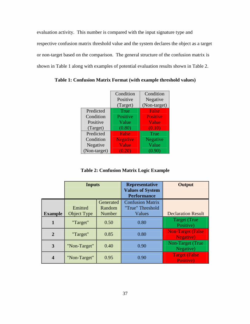
shown in Table 1 along with examples of potential evaluation results shown in Table 2.
Table 1: Confusion Matrix Format (with example threshold values)
Condition Positive (Target)
Condition Negative
(Non-target) Predicted Condition Positive (Target)
True Positive Value (0.80)
False Positive Value (0.10)
Predicted Condition Negative
(Non-target)
False Negative
Value (0.20)
True Negative
Value (0.90)
Table 2: Confusion Matrix Logic Example
Inputs Representative Values of System
Performance
Output
Example Emitted
Object Type
Generated Random Number
Confusion Matrix "True" Threshold
Values Declaration Result
1 "Target" 0.50 0.80 Target (True Positive)
2 "Target" 0.85 0.80 Non-Target (False Negative)
3 "Non-Target" 0.40 0.90 Non-Target (True Negative)
4 "Non-Target" 0.95 0.90 Target (False Positive)

38
If a "target" declaration is made, the model generates a trigger simulating data
transfer to a ground control station for potential action, specifics of which are outside the
scope of this effort. After completing either a simulated data transfer or a "non-target"
declaration, the simulation checks for a mission status of "recovery" and selects to either
resume search or end sensor operations if recovery is set to true.
3.8.3 Variation 2 Operation
The partial OV-5b of Variant 2, as shown in Figure 7, is very similar to Variant 1
with the exception that each UAS has a dedicated GCS node. The duration of the sensor
data transfer is now represented as a triangular distribution rather than an assumed
constant time interval, as in Variant 1. Simulation of the sensor performance is the same
as described in Variant 1.
The additional process where the ground station simulates evaluation of the data
that is received is also depicted in the OV-5b. This operation is modeled in the same
manner as the sensor's evaluation step described in Variant 1, although new confusion
matrix values may be used, under the premise that a human analyst will be confirming or
rejecting targets under differing criteria compared to the onboard sensor. Once the object
data is evaluated and the ground station then either confirms or rejects the target, the GCS
waits for another data set to be transferred.

39
Figure 7: Variant 2, Partial OV-5b

40
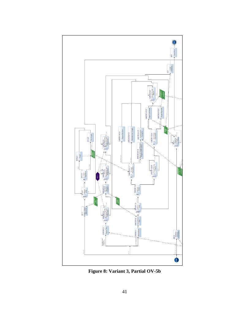
3.8.4 Variant 3 Operation
Variant 3, shown in Figure 8, operates in a cooperative manner to provide a
confirmatory step. The addition of a "Sensor Mode" decision checks for a valid request
from a cooperative UAS to determine if it will begin standard search operations or
perform a target confirmation action. In the condition of no confirmation requests
present, the system awaits an object signature and performs an evaluation as previously
described. In the event an object is declared a target, the UAS requests confirmation
otherwise it returns to check for a confirmation request and begins the cycle over.
If there is a confirmation request, a triangular distribution sets a transit time to and
from the requesting UAS. After the transit time is simulated, the sensor simulates an
evaluation and either confirms or rejects the target. If confirmed, the UAS simulates a
basic data transfer to the ground station and both UAS resume search operations, with the
confirming UAS allowing for time to transit back to its original mission area. If during
return transit, the UAS in search mode requests an additional confirmation, the transiting
UAS returns to confirm as before, assuming the same transit duration as executing during
its return transit to that point.
41
Figure 8: Variant 3, Partial OV-5b

42
3.9 Evaluation for Model Completeness
Since the architecture was the basis for the simulation model, the simulation order
of events and decision points must inherently match the architecture. This characteristic
is a clear advantage of development of an architecture on a platform that facilitates direct
simulation. However, since there is a level of abstraction used in the architecture, there
may be operational parameters and/or assumptions that are not explicitly defined within
standard architecture views, yet are required for a representative simulation. A brief
discussion of these parameters was shown previously in the variant operations.
Additionally, as previously discussed, simulation of external stimuli that are beyond the
scope of a system's architecture definition may be required for the EA to simulate
properly. Evaluation of MOE results, requirements, and key parameters are the final step
of the ABEP and are discussed in chapter 4.
3.10 Test Case Selection
With the core architecture and simulation details defined, relevant test cases were
selected. The desire was to present what were deemed reasonable scenarios in order to
indicate system performance and aid in selection of a variant for continued development.
While many more parameters were available for manipulation, parameters that were
varied for this thesis were limited to Target Density and Sensor Target Detection
Threshold. Each parameter was varied at two levels, providing 12 unique test cases
across all three variants. A test case summary matrix is shown in Table 3.

43
Table 3: Test Case Matrix
Test Case Target to Non-Target Density
Sensor Target Detection Threshold
1 1:2 Low 2 1:2 High 3 1:20 Low 4 1:20 High
Target density was modeled by adjusting the rate at which the object activity
generated targets versus the rate of non-target generation. In this case, target to non-
target ratios of 1:2 and 1:20 were selected to represent a target rich environment and a
sparse target environment, respectively. For the target rich environment, a generated
value of less than the value of 1/3 equated to a target emission, where as a value greater
than 1/3 resulted in emission of a non-target emission, and similarly, the sparse target
environment was assigned a threshold of 1/21.
The confusion matrices for the UAS sensor considered for this thesis are shown
below in Table 4 and Table 5. The intent is to represent the same sensor with differing
target detection threshold values. A sensor of the same capabilities was chosen because it
is assumed that a sensor with increased capabilities across all areas will therefore perform
better under all scenarios. The terms low- and high-target detection threshold represent a
value of confidence at which a target declaration is made. A higher target detection
threshold represents a lower false positive rate but a higher missed target rate and the
opposite is true for a low target detection threshold. This notion is not intuitive when
looking solely at the respective rates for true positives and true negatives, i.e. the low

44
target detection threshold confusion matrix contains more stringent requirements for a
true positive declaration.
Table 4: Sensor Low Target Detection Threshold Confusion Matrix
Condition Positive (Target)
Condition Negative
(Non-target) Predicted Condition Positive (Target)
0.80 0.10
Predicted Condition Negative
(Non-target)
0.20 0.90
Table 5: Sensor High Target Detection Threshold Confusion Matrix
Condition Positive (Target)
Condition Negative
(Non-target) Predicted Condition Positive (Target)
0.75 0.05
Predicted Condition Negative
(Non-target)
0.25 0.95
In the case of Variant 2, the GCS was deemed to possess a better capability to
evaluate objects and thus was assigned a more accurate confusion matrix, as shown in
Table 6. The GCS confusion matrix was not varied between test cases.

45
Table 6: Ground Control Station Confusion Matrix
Condition Positive (Target)
Condition Negative
(Non-target) Predicted Condition Positive (Target)
0.85 0.05
Predicted Condition Negative
(Non-target)
0.15 0.95
3.11 Other Model Parameters
The models were built with multiple other fixed parameters, presented in Table 7.
The other model parameters were not changed within the data collection for this thesis
they are available for modification in any future exploration into this architecture. All
additional parameters were selected based on values deemed reasonable for the intended
use of the UAS.
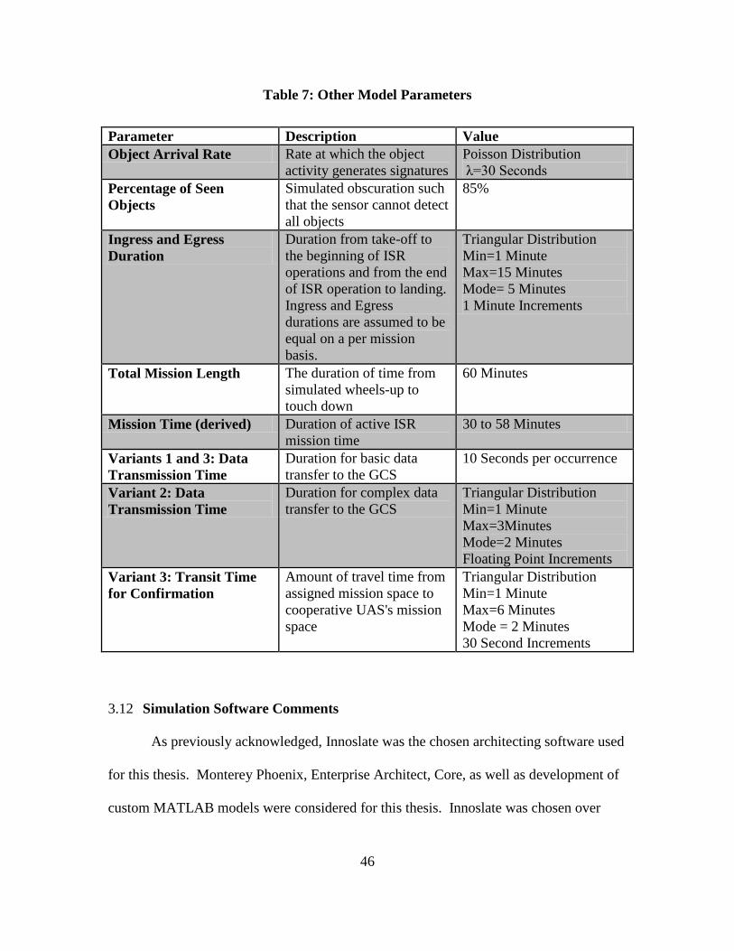
46
Table 7: Other Model Parameters
Parameter Description Value Object Arrival Rate Rate at which the object
activity generates signatures Poisson Distribution λ=30 Seconds
Percentage of Seen Objects
Simulated obscuration such that the sensor cannot detect all objects
85%
Ingress and Egress Duration
Duration from take-off to the beginning of ISR operations and from the end of ISR operation to landing. Ingress and Egress durations are assumed to be equal on a per mission basis.
Triangular Distribution Min=1 Minute Max=15 Minutes Mode= 5 Minutes 1 Minute Increments
Total Mission Length The duration of time from simulated wheels-up to touch down
60 Minutes
Mission Time (derived) Duration of active ISR mission time
30 to 58 Minutes
Variants 1 and 3: Data Transmission Time
Duration for basic data transfer to the GCS
10 Seconds per occurrence
Variant 2: Data Transmission Time
Duration for complex data transfer to the GCS
Triangular Distribution Min=1 Minute Max=3Minutes Mode=2 Minutes Floating Point Increments
Variant 3: Transit Time for Confirmation
Amount of travel time from assigned mission space to cooperative UAS's mission space
Triangular Distribution Min=1 Minute Max=6 Minutes Mode = 2 Minutes 30 Second Increments
3.12 Simulation Software Comments
As previously acknowledged, Innoslate was the chosen architecting software used
for this thesis. Monterey Phoenix, Enterprise Architect, Core, as well as development of
custom MATLAB models were considered for this thesis. Innoslate was chosen over

47
these programs due to the availability of licensing, preservation of concordance within
the architecture, integrated simulations, and overall ease of use. That said the software
had some shortfalls. First, the cloud version of Innoslate used for this thesis is not able to
perform Monte Carlo simulations currently. The developers have a beta version of their
cloud Monte Carlo simulation available but it did not successfully execute the models
developed for this thesis. Furthermore, information on Monte Carlo default settings or
the ability to adjust the number of trials was available for the simulations. Second, output
of simulation results to a file was not natively available and thus results were manually
transferred to a program, in this case MS Excel, for analysis. The simulation runs on a
JavaScript platform, which is user-friendly for model generation but inherently does not
allow file generation on a client machine. The inability to capture output data in separate
files severely limits the scaling capabilities of the program. Finally, triggers must be
dealt with care and deliberation within the simulations. In a static activity diagram,
triggers should occur wherever completion if an activity permits activation of another
activity. This became a problem during simulation, specifically for loops. In cases
where triggers were used to activate looping activities, the completion and exit of the
loop stimulus activity caused the simulation to fail to execute since the looping activity
was still waiting for a trigger. The failure to complete simulation can be avoided but
creates extra steps and/or activities not pertinent at the level of abstraction used for the
activity diagram.

48
3.13 Summary
This chapter detailed the application of the ABEP process to the architecture
under development with exception of step 8 which will be completed and commented
upon in chapter 4.
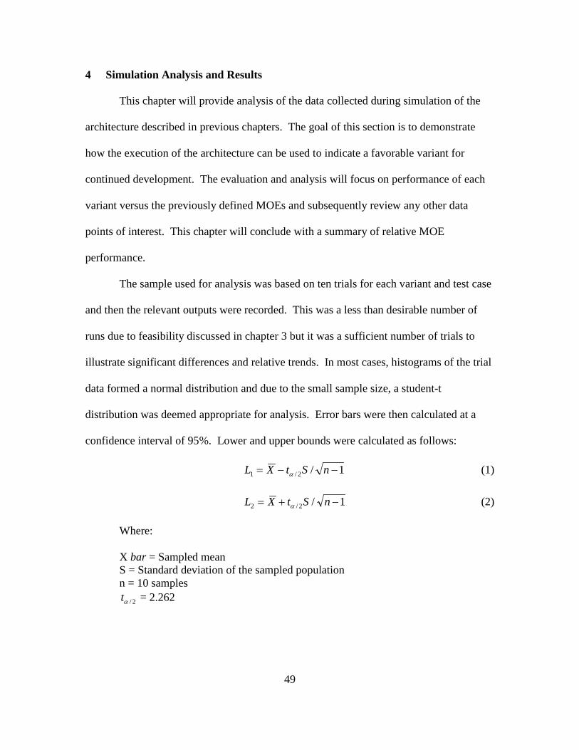
49
4 Simulation Analysis and Results
This chapter will provide analysis of the data collected during simulation of the
architecture described in previous chapters. The goal of this section is to demonstrate
how the execution of the architecture can be used to indicate a favorable variant for
continued development. The evaluation and analysis will focus on performance of each
variant versus the previously defined MOEs and subsequently review any other data
points of interest. This chapter will conclude with a summary of relative MOE
performance.
The sample used for analysis was based on ten trials for each variant and test case
and then the relevant outputs were recorded. This was a less than desirable number of
runs due to feasibility discussed in chapter 3 but it was a sufficient number of trials to
illustrate significant differences and relative trends. In most cases, histograms of the trial
data formed a normal distribution and due to the small sample size, a student-t
distribution was deemed appropriate for analysis. Error bars were then calculated at a
confidence interval of 95%. Lower and upper bounds were calculated as follows:
1/2/1 −−= nStXL α (1)
1/2/2 −+= nStXL α (2)
Where:
X bar = Sampled mean S = Standard deviation of the sampled population n = 10 samples
2/αt = 2.262
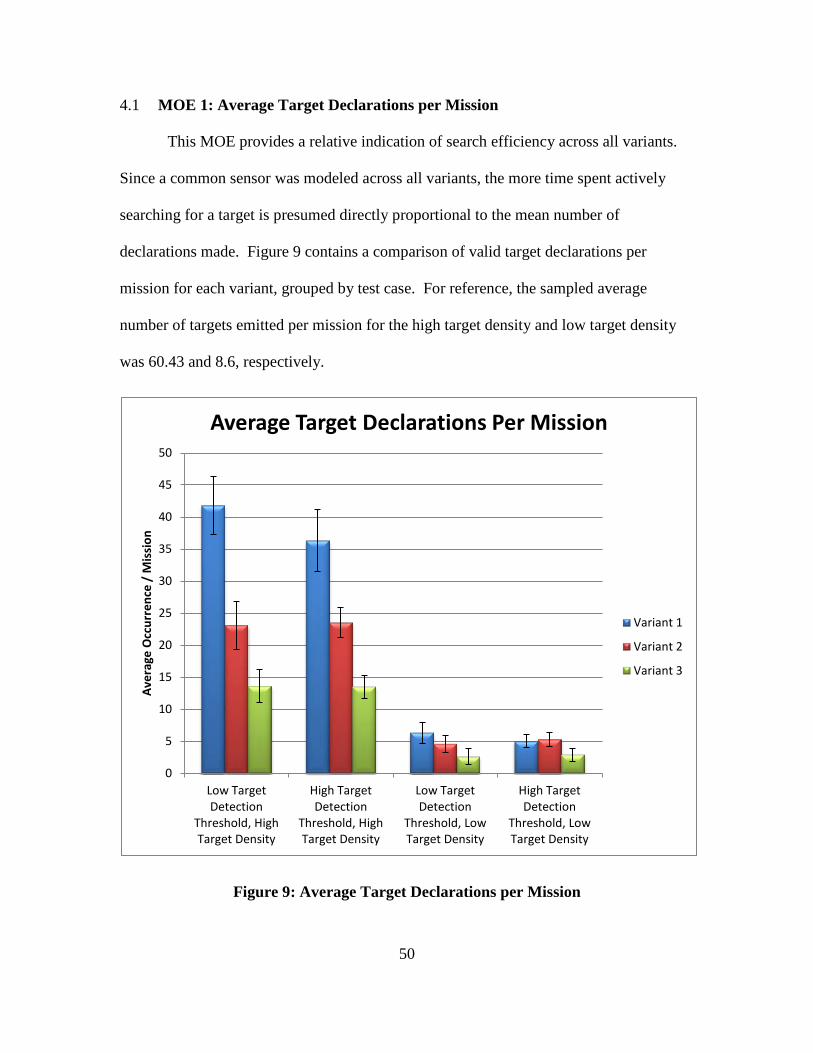
50
4.1 MOE 1: Average Target Declarations per Mission
This MOE provides a relative indication of search efficiency across all variants.
Since a common sensor was modeled across all variants, the more time spent actively
searching for a target is presumed directly proportional to the mean number of
declarations made. Figure 9 contains a comparison of valid target declarations per
mission for each variant, grouped by test case. For reference, the sampled average
number of targets emitted per mission for the high target density and low target density
was 60.43 and 8.6, respectively.
Figure 9: Average Target Declarations per Mission
0
5
10
15
20
25
30
35
40
45
50
Low Target Detection
Threshold, High Target Density
High Target Detection
Threshold, High Target Density
Low Target Detection
Threshold, Low Target Density
High Target Detection
Threshold, Low Target Density
Aver
age
Occ
urre
nce
/ M
issi
on
Average Target Declarations Per Mission
Variant 1
Variant 2
Variant 3

51
In the cases of high target density, all variants demonstrated a statistically
significant difference in detections per mission at the 95% confidence interval. The
respective lower declaration rates of Variants 2 and 3 when compared to Variant 1 are
presumed to be a result of evaluating fewer total objects. In these cases, Variants 2 and 3
are sending sensor data or transiting to confirm an object, respectively, instead of
evaluating additional objects. Conversely, Variant 1 spends much more time actively
evaluating objects and thus generally has higher overall declaration rates. An interesting
observation is noted when comparing individual variant declaration performance in the
high target density cases. While the declaration rate for Variant 1 trends downward as
the target density is reduced and target detection thresholds is raised, this trend is not
apparent for Variants 2 and 3. A possible explanation is that in these cases, valid targets
are relatively prevalent; leading to frequent data transmission and transit delays, thus
resulting in a small impact from the change in target detection threshold.
In the cases of low target density, only Variants 1 and 3 displayed a statistical
difference at a low target detection threshold while both Variants 1 and 2 were
statistically better than Variant 3 for the high target detection threshold. When
comparing the relative effect of target density to declaration performance of all cases,
Variants 2 and 3 in a low target density scenario are, on a percentage basis, much closer
to that of Variant 1 than that same comparison in the high target density cases. This
indicates that the declaration performance of Variant 1 declines faster than that of
Variants 2 and 3 as the target density reduces.

52
4.2 MOE 2: Average Target Confirmations per Mission
As described in chapter 3, Variants 2 and 3 perform an additional confirmation
step with the primary objective of reducing false alarm rates. This MOE provides an
indication of which variant produces more confirmations per mission. Reviewing Figure
10 reveals a significant performance advantage, at a 95 % confidence, for Variant 2 in all
high target density scenarios but the significance is lost in low target density scenarios.
Given that the quantity of object signature inputs to the confirmation process are a
direct result of the number of declarations, the result of fewer variant 3 declarations is in
line with expectations although the statistical difference is lost for the high target
detection, low target density case. Additionally, the lack of statistical difference from test
case to test case for Variant 3 within the same target density group indicates that the
target density is much more influential in these cases than the target detection threshold.
Given the declaration rates shown in Figure 9, Variant 2 should not show a statistical
difference as the confirmation step occurs in the GCS and therefore always uses the same
target detection thresholds.
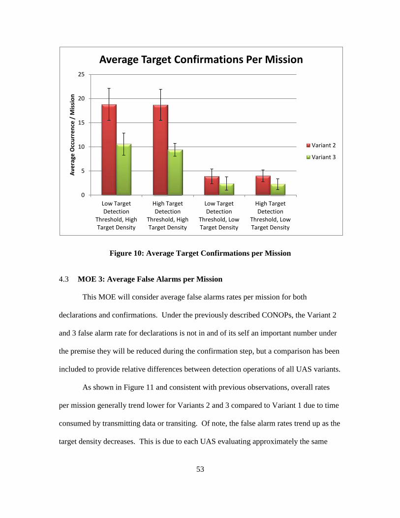
53
Figure 10: Average Target Confirmations per Mission
4.3 MOE 3: Average False Alarms per Mission
This MOE will consider average false alarms rates per mission for both
declarations and confirmations. Under the previously described CONOPs, the Variant 2
and 3 false alarm rate for declarations is not in and of its self an important number under
the premise they will be reduced during the confirmation step, but a comparison has been
included to provide relative differences between detection operations of all UAS variants.
As shown in Figure 11 and consistent with previous observations, overall rates
per mission generally trend lower for Variants 2 and 3 compared to Variant 1 due to time
consumed by transmitting data or transiting. Of note, the false alarm rates trend up as the
target density decreases. This is due to each UAS evaluating approximately the same
0
5
10
15
20
25
Low Target Detection
Threshold, High Target Density
High Target Detection
Threshold, High Target Density
Low Target Detection
Threshold, Low Target Density
High Target Detection
Threshold, Low Target Density
Aver
age
Occ
urre
nce
/ M
issi
on
Average Target Confirmations Per Mission
Variant 2
Variant 3

54
number of objects with fewer valid targets in that group and therefore an increased
opportunity to declare more false alarms exists.
In this data set, there is never a statistically significant performance difference
between Variants 1 and 2 although there is a consistent trend of higher average false
alarms per mission for Variant 1. Variant 3 performed statistically better than Variants 1
and 2 in all cases except the low target threshold, high target density case.
Figure 11: Average False Alarm Declarations per Mission
0
2
4
6
8
10
12
14
16
18
20
Low Target Detection
Threshold, High Target Density
High Target Detection
Threshold, High Target Density
Low Target Detection
Threshold, Low Target Density
High Target Detection
Threshold, Low Target Density
Aver
age
Occ
urre
nce
/ M
issi
on
Average Declared False Alarms Per Mission
Variant 1
Variant 2
Variant 3

55
Figure 12 contains false alarms that make it through both declaration and
confirmation evaluations. Note that Variant 2 confirmed zero false alarms for the high
detection threshold, high target density case and thus a confidence interval based on a
normal distribution was not appropriate. In this case a "Rule of 3" confidence interval
was deemed an appropriate method for approximating a confidence interval.
With respect to the Variant 2 high target threshold and high target density test
case, there are two reasons why a value of zero is not unreasonable. First, as shown in
Figure 13, a relatively small number of false positives were flagged for a confirmatory
look, reducing overall probability that one or more false alarms are confirmed. Second,
and as mentioned previously, the GCS confusion matrix used represents a highly accurate
evaluation. These traits combined lead to a very low probability of a false alarm
confirmation.
The data for false alarm confirmations frequently contains zero confirmations per
mission, creating a dataset skewed towards zero. Given the small sample size, this
appeared to cause larger than reasonable confidence intervals using normal distribution
confidence interval methods. Non-parametric methods were evaluated for determining
appropriate confidence intervals however none indicated a statistically significant
performance difference among any test case.
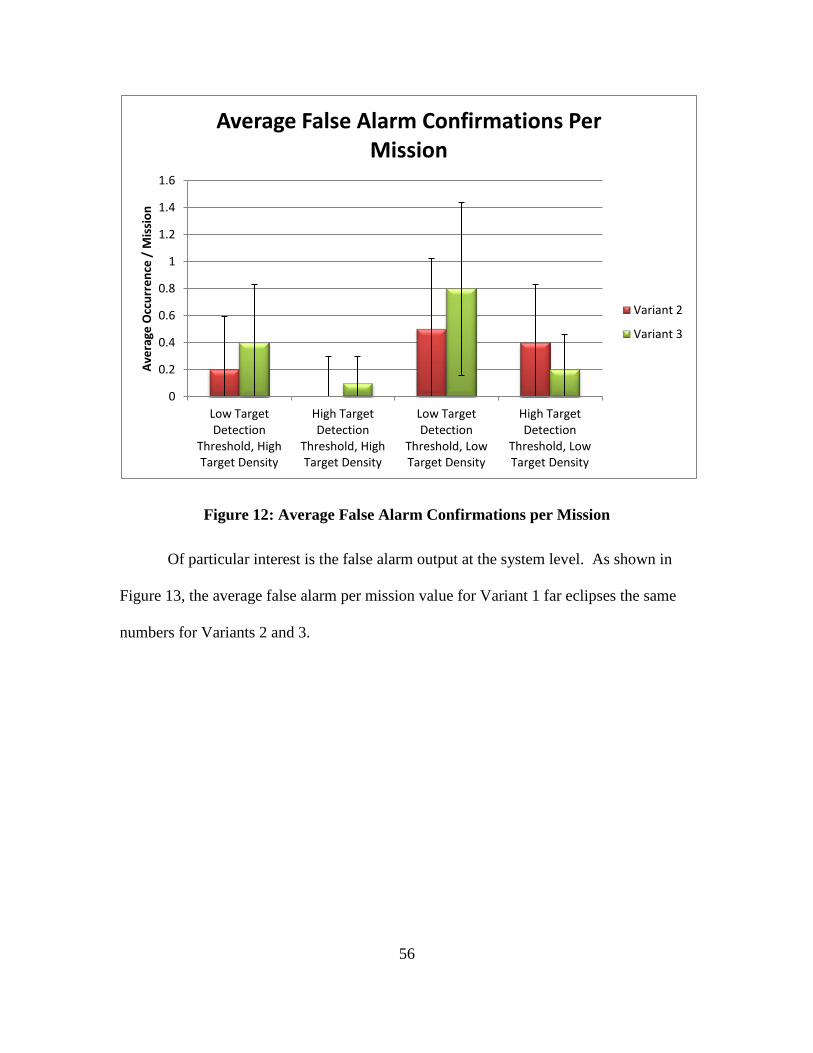
56
Figure 12: Average False Alarm Confirmations per Mission
Of particular interest is the false alarm output at the system level. As shown in
Figure 13, the average false alarm per mission value for Variant 1 far eclipses the same
numbers for Variants 2 and 3.
0
0.2
0.4
0.6
0.8
1
1.2
1.4
1.6
Low Target Detection
Threshold, High Target Density
High Target Detection
Threshold, High Target Density
Low Target Detection
Threshold, Low Target Density
High Target Detection
Threshold, Low Target Density
Aver
age
Occ
urre
nce
/ M
issi
on
Average False Alarm Confirmations Per Mission
Variant 2
Variant 3
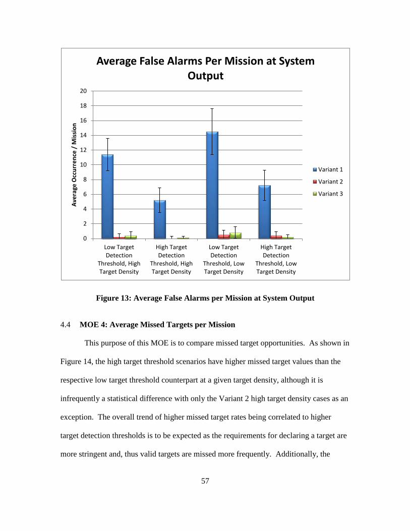
57
Figure 13: Average False Alarms per Mission at System Output
4.4 MOE 4: Average Missed Targets per Mission
This purpose of this MOE is to compare missed target opportunities. As shown in
Figure 14, the high target threshold scenarios have higher missed target values than the
respective low target threshold counterpart at a given target density, although it is
infrequently a statistical difference with only the Variant 2 high target density cases as an
exception. The overall trend of higher missed target rates being correlated to higher
target detection thresholds is to be expected as the requirements for declaring a target are
more stringent and, thus valid targets are missed more frequently. Additionally, the
0
2
4
6
8
10
12
14
16
18
20
Low Target Detection
Threshold, High Target Density
High Target Detection
Threshold, High Target Density
Low Target Detection
Threshold, Low Target Density
High Target Detection
Threshold, Low Target Density
Aver
age
Occ
urre
nce
/ M
issi
on
Average False Alarms Per Mission at System Output
Variant 1
Variant 2
Variant 3

58
observation of fewer missed targets in lower target density environments is an artifact of
the existence of fewer targets to miss.
Figure 14: Average Missed Target Declarations per Mission
Figure 15 shows the average post-confirmation missed targets per mission values. This
dataset only represents objects that have successfully passed a declaration evaluation as a
true positive or a false positive and therefore have no relation to the missed targets
identified in Figure 14.
0
2
4
6
8
10
12
14
16
Low Target Detection
Threshold, High Target Density
High Target Detection
Threshold, High Target Density
Low Target Detection
Threshold, Low Target Density
High Target Detection
Threshold, Low Target Density
Aver
age
Occ
urre
nce
/ M
issi
on
Average Missed Target Declarations Per Mission
Variant 1
Variant 2
Variant 3
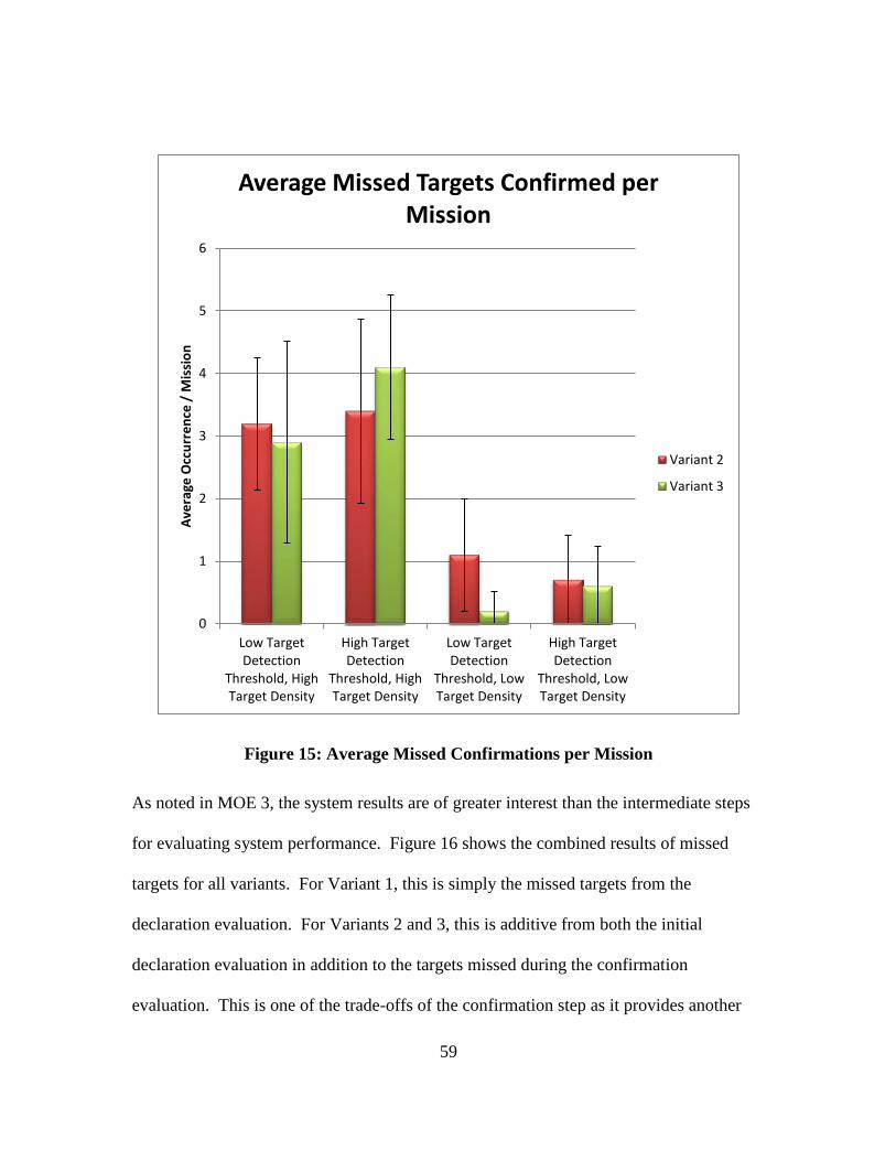
59
Figure 15: Average Missed Confirmations per Mission
As noted in MOE 3, the system results are of greater interest than the intermediate steps
for evaluating system performance. Figure 16 shows the combined results of missed
targets for all variants. For Variant 1, this is simply the missed targets from the
declaration evaluation. For Variants 2 and 3, this is additive from both the initial
declaration evaluation in addition to the targets missed during the confirmation
evaluation. This is one of the trade-offs of the confirmation step as it provides another
0
1
2
3
4
5
6
Low Target Detection
Threshold, High Target Density
High Target Detection
Threshold, High Target Density
Low Target Detection
Threshold, Low Target Density
High Target Detection
Threshold, Low Target Density
Aver
age
Occ
urre
nce
/ M
issi
on
Average Missed Targets Confirmed per Mission
Variant 2
Variant 3

60
opportunity to miss or discard valid targets. While none of the results represent a
statistically significant difference, it is unexpected to see that the sample mean of Variant
2 is larger than that of Variant 1 for the low target density thresholds, especially given the
more accurate confusion matrix used to simulate the GCS confirmation.
Figure 16: Total Average Missed Targets per Mission
4.5 Other Observations
For Variant 1, object evaluation rates are generally around 85%, which was the
selected rate at which obscuration prevents detection of an object. However, Variants' 2
and 3 object evaluation rates trend upward as target density is reduced and target
0
2
4
6
8
10
12
14
16
Low Target Detection
Threshold, High Target Density
High Target Detection
Threshold, High Target Density
Low Target Detection
Threshold, Low Target Density
High Target Detection
Threshold, Low Target Density
Aver
age
Occ
urrr
ence
/ M
issi
on
Total Average Missed Targets per Mission
Vatiant 1
Variant 2
Variant 3

61
detection threshold values are increased. Since confirmation steps are only performed on
declared targets, a sparse target environment or a higher rejection of false alarms leads to
a relative increase in mission time spent on evaluation and thus an increase in evaluation
rates.
Figure 17 illustrates that concept in action but also provides trend indications on
rates of change. Target detection threshold does not significantly affect evaluation rates
in an already dense target population however in both the cases of Variants 2 and 3, it is a
significant factor in low target threshold scenarios.
Figure 17: Average Evaluation Rates per Mission
0.0%
10.0%
20.0%
30.0%
40.0%
50.0%
60.0%
70.0%
80.0%
90.0%
100.0%
Low Target Detection
Threshold, High Target Density
High Target Detection
Threshold, High Target Density
Low Target Detection
Threshold, Low Target Density
High Target Detection
Threshold, Low Target Density
Obj
ects
Eva
luat
ed/O
bjec
ts E
mitt
ed
Average Evaluation Rates Per Mission
Variant 1
Variant 2
Variant 3

62
4.6 Results
Based on performance against all MOEs, variants were compared against one
another to determine a preferred variant for further development. A summary of results
is shown in Table 8. Note, for MOEs 3 and 4, ratings were performed at the system level.
The relative scoring repeats itself in each of the high and low target density scenarios
with exception of Variant 2, MOE 1 in the low target density, high target detection
threshold case. While there are different absolute levels of performance, the relative
performance is duplicated for both the high and low target detection threshold. This
indicates that, at least in the current model and test cases, target detection threshold does
not significantly affect relative performance and perhaps another variable should be
selected for future study.
Table 8: Evaluation Results Summary
High Target Density Low Target Density High Target
Detection Threshold
Low Target Detection Threshold
High Target Detection Threshold
Low Target Detection Threshold
MO
E 1
MO
E 2
MO
E 3
MO
E 4
MO
E 1
MO
E 2
MO
E 3
MO
E 4
MO
E 1
MO
E 2
MO
E 3
MO
E 4
MO
E 1
MO
E 2
MO
E 3
MO
E 4
V1 - - - - V2 - - - - - - - V3 - - - - - - Legend Statistically Significant High Performer Statistically Significant Mid-Range Performer Statistically Significant Low Performer No Data Set
- Not Able to Rate Due to No Statistical Difference Found

63
In an actual down select process, evaluation criteria need to be rigorously selected
along with weighting factors, the process of which is beyond the scope of this thesis.
However, assuming all MOEs are equally weighted, the relative results of the executable
architecture used for this thesis suggest that Variant 2 is the best overall choice to
continue with for further refinement.

64
5 Conclusions and Recommendations
The purpose of this thesis was to demonstrate how an executable architecture may
be applied to an early concept and use the results to make a decision on how to proceed
with system development. The provided mission was an ISR UAS tasked with detecting
valid targets. A CONOPs and three partially representative architectures were built in a
program capable of performing executable architecture functions. These architectures
were simulated and the results analyzed for statistical differences that were used to
indicate a preference of variants for further development.
At the onset of this thesis, three questions were posed by the author. Those
questions and answers are as follows:
Research Question 1: What is the capability of current architecture modeling
tools to execute simulations directly from a system architecture?
As discovered and commented on during the literature review portion of
this thesis, there is apparent interest in executable architectures from the broad
Systems Engineering Community, but very few integrated software packages
capable of producing valid DoDAF products and executing models with
sufficient fidelity to be useful for decision making. The tool used in this thesis,
Innoslate, appears to be one of the only integrated tools; however the simulation is
not currently capable of Monte Carlo simulations nor does the output lend its self
well to quantitative analysis.

65
Research Question 2: What type of information can be provided from use of an
executable architecture in support of trade space decisions during early concept
development?
The answer to this question is dependent on the fidelity of model and the
ability to access the data to determine statistically significant differences in
operation. The effort undertaken in this thesis produced a basic model with only
four MOEs, three variants and two varied parameters. With only 10 trial runs per
test case and variant, the result was a relative difference in performance could be
demonstrated at a significant level in many cases. If performance predictions are
desired, a more detailed and complete model must be built. Additionally, more
trial runs are required along with a rigorous assessment of parameters varied and
scenarios to ensure the simulation represents an accurate environment.
Research Question 3: How detailed of an executable model is required to
effectively evaluate trade space decisions in early concept modeling?
As demonstrated in chapter 4, the model created for this thesis was
sufficient to indicate a preferred solution based on the information entered into the
architecture model. A basic yet representative model was created in a commercial
modeling program and provided sound data output based on the conditions and
the inputs. Moreover, through data analysis, the limiting factors of the modeled
system become apparent. For instance, Variant 3 appears to be an efficient
solution on paper. The model consistently demonstrated poor performance
compared to the competing variants; however, the data indicated that transit times

66
were severely lowering available time to perform new object evaluations.
Conversely, Variant 1 had relatively high evaluation efficiency but suffered from
higher system level false alarms. When deciding how to proceed, consideration
should be given to the cost, schedule and performance risk of a faster Variant 3
UAS, thereby reducing transit time; a more accurate Variant 2 sensor, reducing
false alarms and missed targets or a change in CONOPS for one or both variants.
5.1 Recommendations for Future Research
5.1.1 Larger SoS Development
Recommend that future work expand SoS modeling to include heterogeneous
vehicles and a larger quantity of systems such that effects of emerging behavior may be
modeled and studied. An addition of a larger task set and additional logic in the system
would help model a more realistic environment and is more representative of a state of
the art system.
5.1.2 Improve Existing Simulation Assumptions
Model object signature emissions in a spatial distribution rather than the arrival
rate method used in this thesis. This will require significant advancements in the existing
executable architecture programs but will provide a more realistic scenario.
5.1.3 Include More External Factors
External costs weren't explicitly considered in this thesis. For instance, from a UAS
MOE perspective, Variant 2 appeared to be the highest performer however in practice, it

67
will require significantly more bandwidth and additional analyst personnel that were not
considered in the selection process.

68
Appendix A: CONOPS
Document Overview
This document describes a concept of operations (CONOPS) for a fictitious small
unmanned aerial system (UAS).
Intended Users
This document is intended for stakeholders and reviewers in the architecture
development process for the system under design.
Document Organization
• Section 1 describes the document format and intended users.
• Section 2 describes the purpose of the UAS system, functional requirements,
stakeholders, and their relationships.
• Section 3 provides a physical description of the UAS.
• Section 4 describes and operational description of the UAS.
• Section 5 provides an acronym list
System Introduction
This section will describe the purpose of the UAS system, functional
requirements, stakeholders, and their relationships.
System Purpose
The Combatant Commander (COCOM), with responsibility over a given area, has
a requirement to discover, to the maximum practical extent, all valid targets for the
69
purposes of further surveillance and/or subsequent engagement and is in need of a system
to help meet this requirement. Therefore, the purpose of this UAS system is to detect
objects in a given mission area and determine if those objects are valid targets to the
greatest extent possible. The target location and validation information will be used by
the COCOM to cue additional platforms for long term surveillance and/or engagement.
Functional Requirements
This section describes some of the tasks the system must perform from a
functional perspective to achieve mission success.
Target Detection
The system must be able to accurately detect targets in a varied and unpredictable
physical environment.
Communications
The system must transfer sufficient quantities of information to a ground control
station (GCS) or other assets to identify target location and in some cases, raw data for
confirmatory analysis.
Mobility
The system must move freely throughout the area of interest in order to detect the
maximum possible number of valid targets and in the case of Variant 3, provide target
confirmation.
70
Duration
The system must provide sufficient on-station duration capabilities to complete
the system’s ISR mission and in some cases, allow confirmatory assessments of the target
and to increase overall mission efficiency.
Geo-location accuracy
The system must track field of view location for accurate record of target location
and to prevent excessive overlap of data collection throughout the mission.
Launch and Recovery
The system must navigate to and from the mission area to ensure system re-use.
Stakeholders
Intelligence Community
Data from this UAS will be used for Intelligence Preparation of the Battlespace
(IPB). Information from the platform must be timely and accurate. Data from the UAS
must be provided in a common, recognizable format. Data from the UAS degrades with
time and must be provided as soon as possible to be of the greatest value.
Other ISR Platforms
Other sources may be used for target confirmation. The location of the target
must be accurate to ensure confirmatory information is valid.

71
Airborne Strike Operators and Ground Forces
The UAS must provide accurate target information and not interfere with any
engagement techniques.
Acquisition Corps
A method of system performance feedback must be enabled. This information
will help further system improvements and updates affect increased performance and
reliability.
System Physical Description
The system will consist of 3 major components: Ground Control Station, data
link, and the air vehicle.
Ground Control Station (GCS)
This component of the system is tactical in nature and therefore must be mobile
throughout an area of operations. The GCS contains a networked data storage server in
addition to analyst and mission planning terminals. It has a self-contained HVAC system
and inputs for generator or commercial power. The system also has connections for
external network access.
Data link
This component of the system is consists of a ground based transmitter/receiver
dish, airborne transmitter/receiver dish and interface, communications processing server
72
and all associated connections to the GCS. The transmitter/receiver dishes are capable of
being trailer mounted or mounted on the ground near the trailer within close proximity.
Air Vehicle
This component of the system consists of a small conventional design air vehicle.
The vehicle houses navigation, propulsion, sensor, and communications systems. The
navigation system consists of a GPS sensor, inertial navigation system, mission storage
components, and interfaces to all other subsystems. The propulsion system consists of a
hydrocarbon fueled engine, integrated fuel storage, control system and interface to the
navigation system. The sensor system consists of the physical sensor, autonomous target
recognition hardware, storage system for the target library and interface to the navigation
system. The communications system is the airborne portion of the data link described
previously.
System Operational Description
This section will provide a chronological description of system operations and
requirements for a typical mission. The total flight durations are a set, standard length.
Logistics
The system will be deployed, likely to remote locations by cargo aircraft and/or
ground transportation. Multiple systems may be deployed in the same location and use
the same logistics resources. A spares package will be part of the standard deployment
along with technicians trained to perform pre-flight checks, uploading of mission plans

73
and troubleshoot and repair all foreseeable issues. Fuel is also to be located at the
deployed environment and refueling operations must be performed prior to the
commencement of all missions.
Launch and Ingress
Following successful preparations for flight, the engine is started and the vehicle
prepared for launch and ingress to the mission area. The system is highly automated so
once the ground control station communicates a proceed command, the air vehicle
launches, reaching the pre-programmed operational envelope and proceeds to the mission
area.
Mission Operations
This section will describe standard mission operations for several architecture
variants under consideration.
Variant 1
This variant of the system operates in an autonomous, independent mode. The
system searches for objects using the onboard sensor. Once the sensor identifies an
object, the collected data are run through an autonomous target recognition (ATR)
system. The ATR system processes the data and determines a level of object match to an
existing set of target data. When the matching coefficient is higher than the threshold
value, the coefficient information is then transferred to the ground station for further
action by external entities or stored for later use. At no time under this scenario is the
target confirmed by another source or human analyst.

74
Variant 2
This variant of the system operates in an autonomous mode with human analyst
confirmation. The system searches for objects using the onboard sensor. Once the sensor
identifies an object, the collected data are run through an ATR system. The ATR system
processes the data and determines a level of object match to an existing set of target data.
When the matching coefficient is higher than the threshold value, the coefficient
information, and native sensor data is transferred to the ground station where the data is
analyzed for confirmation by a human analyst.
Variant 3
This variant of the system operates in an autonomous, cooperative mode. The
system searches for objects using the onboard sensor. Once the sensor identifies an
object, the collected data are run through an ATR system. The ATR system processes the
data and determines a level of object match to an existing set of target data. When the
matching coefficient is higher than the threshold value, a request with current location is
then transferred to the nearest cooperative UAS for confirmation. During the time when
the secondary UAS is en route, the primary UAS will continue to track the object. Upon
arrival the secondary UAS observes the object and determines an independent target
coefficient. If the object is determined to be a target, relevant coefficients and locations
are transmitted to the GCS. Upon transfer completion, the primary UAS resumes search
and the secondary UAS returns to its previous search pattern to proceed to search. If the
primary UAS requests another confirmation during transit, the secondary UAS has the
ability to quit transit and return to assist the primary UAS.

75
Egress and Recovery
Once time or fuel for mission operations has expired, all UAS will exit the area of
interest and autonomously navigate to the launch site for recovery. After landing is
accomplished, any recorded data will be downloaded and stored for future reference.
Completion of this step finishes the UAS mission.

76
Appendix B: AV-1
Architectural Description Identification
The architecture under design is the Small Intelligence Surveillance and
Reconnaissance (ISR) Unmanned Aerial System (UAS). The primary purpose of this
system is to support a tactical mission of identifying and providing cueing information
for further tracking or engagement of targets of interest. The system under development
is fictitious but intended to represent a SoS of up to two realistic small UAS that may be
deployed as cooperative or independent systems with varying Ground Control Station
(GCS) reach back capabilities.
This architecture framework will focus on designating parameters of interest to
model future UAS. This framework will be used to represent development decisions in
order to weigh “-ilities” versus cost. The goal is to achieve a high level of system
flexibility, adaptability, and/or robustness while maintaining a predictable life cycle cost
and efficient use of tax payer money.
The architecture is being developed as a thesis project for the Air Force Institute of
Technology (AFIT) in order to demonstrate the use of executable architectures (EA) in
early trade space decision analysis. The architect is Maj Ryan Pospisal, under
advisement and approval of Dr. David Jacques, AFIT faculty. The expected completion
date is December 2015. The anticipated level of effort is 150-200 man-hours.
Assumptions and constraints are as follows:

77
• A commercial tool currently exists, and is accessible to the author, to document a
subset of a DoDAF V2.0 compliant system architecture and includes an
executable modeling capability to meet the fidelity requirements for this thesis.
• Technologies of the representative system are currently attainable or at a level
where it is reasonable that they will be mature enough for implementation by
2025.
• Vulnerabilities to attack, in the physical and cyber domains, are not explicitly
considered or modeled.
• The architecture will be limited in scope due to time constraints and the fictitious
nature of the system.
Scope
The architecture will consist of three distinct variants of the UAS and focus primarily on
identification and development of the operational functionality of the system. Current or
near future technologies are under consideration with an expected 5-10 year horizon.
The architecture development process will closely follow the methods presented
by Dietrichs, et al. that the authors named the Architecture Based Evaluation Process
(ABEP) (Dietrichs et al., 2006). This architecture will focus on the operational aspects of
the system and thus will have limited or no detail on internal system and sub-system
interactions. As such, the preponderance of architecture views will be operational in
nature.
The views created will be limited to those necessary for completing the primary
goals of the project and as such, views will be added, removed, and/or refined as needed
78
to document the necessary system parameters under examination. This architecture will
provide a high-level parametric model, sufficiently detailed to complete early trade space
analysis. Below is a list of anticipated DoDAF viewpoints required for this architecture,
their titles and rationale for their inclusion:
AV-1: Overview and Summary Information
This view is useful for providing an executive level summary of the architecture.
OV-1: High Level Operational Concept Graphic
The OV-1 provides a linkage between physical assets that interact with the system
under development. It provides an abstract depiction of the primary mission activity.
This view provides the reader with an introduction to the CONOP.
OV-2: Operational Resource Flow Description
The OV-2 provides a diagram to show the exchange of resources such as
information, personnel, material, or funding. The OV-2 isn't intended to show
communication links, however in the case of this architecture, the exchange of
information will mimic a communication link.
OV-5b: Operational Activity Model
The OV-5b shows all the high-level activities and chronological linkages between
them. The OV-5b will be the core of this architecture as it lends itself well to simulation
and thus reinforce the concept of an executable architecture.

79
OV-6a: Operational Rules Model
The OV-6a provides rules in a structured English format. These rules form the
basis for how the OV-5b is executed and various decision paths are taken.
Purpose and Perspective
The purpose for this architecture is to produce three system variants and
parametrically model key characteristics of the platforms and their interactions. Once the
variant models are created, they will be formalized to a sufficient level to provide direct
simulation, in the form of an executable architecture. Selected model input parameters
will be varied during the simulations of the resulting EA and the outputs documented
over the course of several iterations of the architecture. Mission specific Measures of
Effectiveness (MOEs) will be developed and used to evaluate the system variants for
selection of the most successful design.
Context
The primary activities of the UAS are launch, perform ingress to the mission area,
perform the ISR mission, egress out of the mission area, and recover to the launch area.
The goals of the CISR platform are to identify and track targets of interest. It will
perform the identification with use of an on-board sensor and Autonomous Target
Recognition (ATR) software. The specifics of sensor type, capabilities, and operation of
the ATR are beyond the scope of this architecture however they will be represented in the
simulation as a uniform random variable processed through a confusion matrix.
Use cases will be developed along with a Concept of Operations (CONOPs) to
assist with generation of the architecture framework. The completed architectures will
80
executed in an architecting software program such as Innoslate to determine parameters
showing greatest impact on “-ilities” of interest. All scenarios and technologies
described in the development of this architecture are either generic or fictitious but are
intended to represent a reasonable application to a UAS ISR mission.
The variants were chosen to provide representative architecture differences to
perform the basic mission of identifying targets and their locations. The intent is that
these differences will produce varied outcomes when executed and facilitate system
design and effective CONOP creation early in a systems' development. Basic
descriptions of the variants are listed as follows:
Variant 1: Automated Independent
This variant of the UAS is an independent system that identifies targets, returns a
matching coefficient and location to the ground control station, and immediately
continues searching for more targets.
Variant 2: Ground Station Assisted
Variant 3 operates similarly to Variant 2, with the exception of confirmation via a
ground control station rather than a cooperative UAS. Confirmation by the ground
station is performed via analysis of sensor data collected by the UAS, sent via a
communications data link. Once object data is collected, the system continues to track
the object until confirmation of a valid target is confirmed by the ground station,
preventing stacking of data sets in the UAS communications cache.

81
Variant 3: Automated Cooperative
This variant searches as described in Variant 1, but upon discovery of a target,
calls a cooperative system to confirm the target as valid. While awaiting arrival of the
cooperative UAS, the primary target continues to "track" the object. Upon target
confirmation, the target description, matching coefficient, and location data are returned
to the ground control station. Both UAS then resume searching for new targets in their
respective original mission areas.
Status
All planned architecture views are complete and capable of being executed within
the Innoslate program.
Tools and File Formats
All written documentation is Microsoft Office compatible. The architecture and
executable portions are based in Innoslate and the model is exportable to an Innoslate
XML file.

82
Appendix C: OV-1: High level Operational Concept Graphic
Figure 18: Variant 1 and Variant 2 OV-1
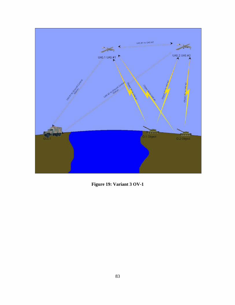
83
Figure 19: Variant 3 OV-1

84
Appendix D: OV-2: Operational Resource Flow Description
Figure 20: Variant 1 OV-2

85
Figure 21: Variant 2 OV-2
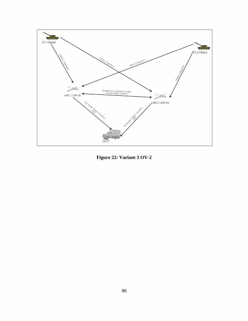
86
Figure 22: Variant 3 OV-2

87
Appendix E: OV-5b: Operational Activity Model
Figure 23: Variant 1 OV-5b

88
Figure 24: Variant 2 OV-5b
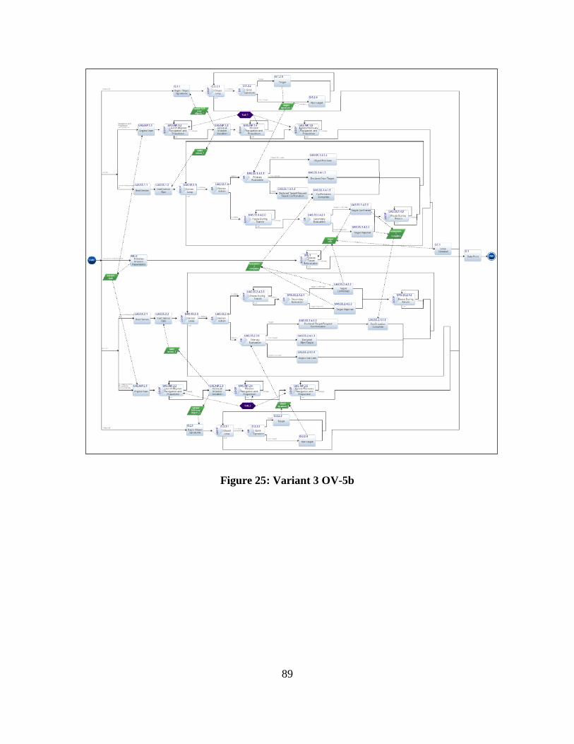
89
Figure 25: Variant 3 OV-5b
90
Appendix F: OV-6a: Operational Rules Model
Due to the similarities of the systems, this OV-6a is divided into four sections:
Common Behavior, Variant 1 Specific Rules, Variant 2 Specific Rules; Variant 3
Specific Rules. Additionally, this architecture is built around a homogeneous two-ship
scenario thus to reduce duplication, only one system is described.
Common Behavior
Assumptions:
Fuel is burned at a steady rate such that duration can be equivocated to amount of
fuel used or required.
Mission plans are loaded prior to UAS launch and all navigation is autonomous.
Imperative Rules
Monitor Fuel Level
Fuel required to return from the assigned mission space to the base shall be
approximated by the amount used to ingress to the mission space. The fuel level
available shall be checked routinely and automatically throughout the mission.
Initialize Mission Parameters
Load mission plans and for purposes of the simulation, sets input parameters and
establishes required variables.
Emits trigger for mission start
Engine Start
Receives mission start trigger to simulate beginning of the propulsion and navigation
subsystem.
91
Boot Sensor
Represents time required for internal sensor checks and when complete, places
sensor in a low power mode until operations is required
Arrive at Mission Location
After completion of Launch and Ingress Propulsion, activates wake sensor
trigger
Start Sensor Ops
Upon receipt of wake sensor trigger, begins sensor operations
Conditional Rules
Launch and Ingress Propulsion
Known: Initial fuel amount, fuel required for launch and mission
If fuel remaining is greater than initial amount minus amount required for
recovery and mission operations,
then continue Launch and Ingress Propulsion.
Else begin Mission Propulsion
Mission Propulsion
Known: Fuel required for mission and recovery operations
If fuel remaining is greater than fuel required for recovery,
then continue Mission Propulsion
else begin Egress and Recovery Propulsion
Egress and Recovery Propulsion
Known: Fuel required for recovery operations
If fuel available is greater than zero,

92
then continue Recovery Propulsion
else End
Variant 1 Specific Rules
Sensor Loop
If recovery propulsion is not active,
then continue to Search and Evaluate Objects
else End
Search and Evaluate Objects
Wait for object signature trigger and evaluate object
If object is declared a target,
then activate target information trigger and transmit basic target information to
Ground Control Station
else return to Sensor Loop
Receive Target Information
Wait for target information trigger
If recovery propulsion is not active,
then continue Receive Target Information
else End
Variant 2 Specific Rules
Conditional Rules
Sensor Loop
93
If recovery propulsion is not active,
then continue to Search and Evaluate Objects
else End
Search and Evaluate Objects
Wait for object signature trigger and evaluate object
If object is declared a target,
then activate object data trigger and transmit detailed object information to
Ground Control Station
else return to Sensor Loop
Receive Data
Wait for target information trigger
If recovery propulsion is not active,
then continue Evaluate Data
else End
Evaluate Data
If data evaluation determines object is a target,
then confirm target and return to Receive Data
else reject target and return to Receive Data
Variant 3 Specific Rules
Search Loop
If recovery propulsion is not active,
then continue to Sensor Mode
94
else End
Sensor Mode
If sensor confirmation request is true
then continue to Secondary Evaluation
else continue to Primary Evaluation
Primary Evaluation
If evaluation results in a target declaration,
then proceed to Declared Target/Request Target Confirmation
else declare non target and return to Sensor Loop
Declared Target/Request Target Confirmation
Send location information to cooperative UAS and continue to Confirmation
Complete
Confirmation Complete
Await evaluation complete trigger and return to Sensor Loop
Secondary Evaluation
If evaluation results in target declaration,
then activate target information trigger and evaluation complete trigger
else activate evaluation complete trigger
return to Sensor Loop
Receive Target Information
Wait for target information trigger
If recovery propulsion is not active,
then continue Receive Target Information

95
else End
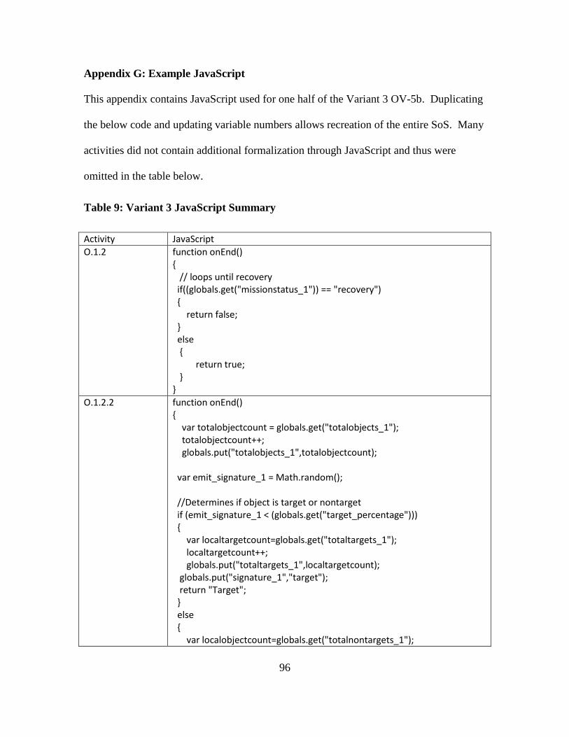
96
Appendix G: Example JavaScript
This appendix contains JavaScript used for one half of the Variant 3 OV-5b. Duplicating
the below code and updating variable numbers allows recreation of the entire SoS. Many
activities did not contain additional formalization through JavaScript and thus were
omitted in the table below.
Table 9: Variant 3 JavaScript Summary
Activity JavaScript O.1.2 function onEnd()
{ // loops until recovery if((globals.get("missionstatus_1")) == "recovery") { return false; } else { return true; } }
O.1.2.2 function onEnd() { var totalobjectcount = globals.get("totalobjects_1"); totalobjectcount++; globals.put("totalobjects_1",totalobjectcount); var emit_signature_1 = Math.random(); //Determines if object is target or nontarget if (emit_signature_1 < (globals.get("target_percentage"))) { var localtargetcount=globals.get("totaltargets_1"); localtargetcount++; globals.put("totaltargets_1",localtargetcount); globals.put("signature_1","target"); return "Target"; } else { var localobjectcount=globals.get("totalnontargets_1");
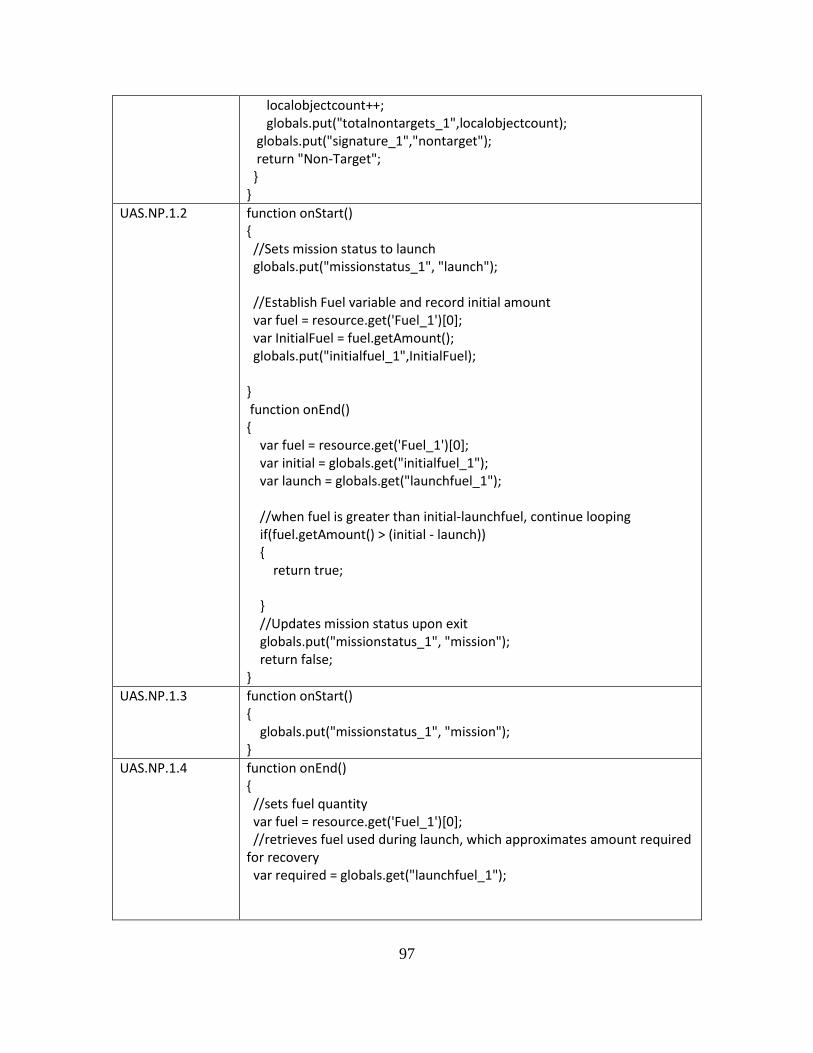
97
localobjectcount++; globals.put("totalnontargets_1",localobjectcount); globals.put("signature_1","nontarget"); return "Non-Target"; } }
UAS.NP.1.2 function onStart() { //Sets mission status to launch globals.put("missionstatus_1", "launch"); //Establish Fuel variable and record initial amount var fuel = resource.get('Fuel_1')[0]; var InitialFuel = fuel.getAmount(); globals.put("initialfuel_1",InitialFuel); } function onEnd() { var fuel = resource.get('Fuel_1')[0]; var initial = globals.get("initialfuel_1"); var launch = globals.get("launchfuel_1"); //when fuel is greater than initial-launchfuel, continue looping if(fuel.getAmount() > (initial - launch)) { return true; } //Updates mission status upon exit globals.put("missionstatus_1", "mission"); return false; }
UAS.NP.1.3 function onStart() { globals.put("missionstatus_1", "mission"); }
UAS.NP.1.4 function onEnd() { //sets fuel quantity var fuel = resource.get('Fuel_1')[0]; //retrieves fuel used during launch, which approximates amount required for recovery var required = globals.get("launchfuel_1");
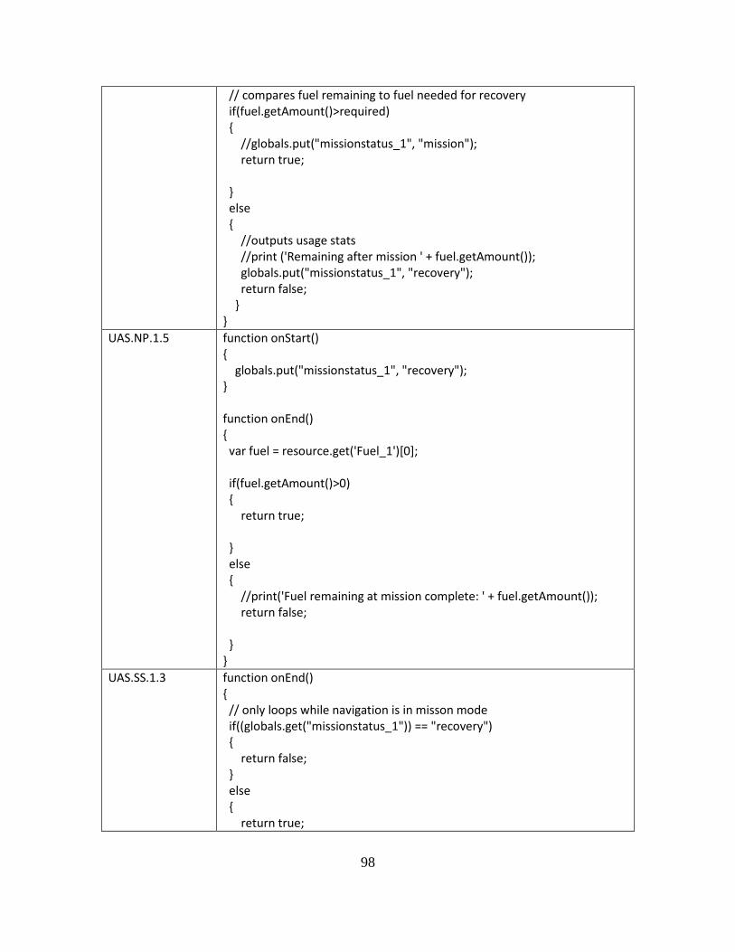
98
// compares fuel remaining to fuel needed for recovery if(fuel.getAmount()>required) { //globals.put("missionstatus_1", "mission"); return true; } else { //outputs usage stats //print ('Remaining after mission ' + fuel.getAmount()); globals.put("missionstatus_1", "recovery"); return false; } }
UAS.NP.1.5 function onStart() { globals.put("missionstatus_1", "recovery"); } function onEnd() { var fuel = resource.get('Fuel_1')[0]; if(fuel.getAmount()>0) { return true; } else { //print('Fuel remaining at mission complete: ' + fuel.getAmount()); return false; } }
UAS.SS.1.3 function onEnd() { // only loops while navigation is in misson mode if((globals.get("missionstatus_1")) == "recovery") { return false; } else { return true;

99
} }
UAS.SS.1.4 function onEnd() { if (globals.get("uas_2_confirmation_request")=="true") { return "Confirm"; } else { return "Search"; } }
UAS.SS.1.4.1.1 function onEnd() { //Retrieve object type var signature_type_1 = globals.get("signature_1"); //Aborts if UAS2 is awaiting confirmation if (globals.get("uas_2_confirmation_request")=="true") { if (signature_type_1 == "target") { var missedtarget_pri_1 = globals.get("missedtarget_1"); missedtarget_pri_1++; globals.put("missedtarget_1", missedtarget_pri_1); } else { var missedobject_pri_1 = globals.get("missedobject_1"); missedobject_pri_1++; globals.put("missedobject_1", missedobject_pri_1); } return "Object Not Seen"; } //initializes variable to determine if object is seen by the sensor var objectseen_1 = Math.random(); var detection = globals.get("detection_percentage"); //proceeds if object is "seen" if (objectseen_1 < detection) { //initialize variable for confusion matrix path

100
var search_confusion_1 = Math.random(); var truepositive = globals.get("truepositive"); var truenegative = globals.get("truenegative"); if(signature_type_1=="target") { if (search_confusion_1 < truepositive) { //counts truepositives var tpcount_pri_1 = globals.get("truepositive_1"); tpcount_pri_1++; globals.put("truepositive_1",tpcount_pri_1); //Stores object type so not over written for human eval globals.put("uaseval_1", signature_type_1); globals.put("uas_1_confirmation_request", "true"); return "Target"; } else { //counts falsenegatives var fncount_pri_1 = globals.get("falsenegative_1"); fncount_pri_1++; globals.put("falsenegative_1",fncount_pri_1); return "Non-target"; } } else { if (search_confusion_1 < truenegative) { //counts truenegatives var tncount_pri_1 = globals.get("truenegative_1"); tncount_pri_1++; globals.put("truenegative_1",tncount_pri_1); return "Non-target"; } else { //counts falsepositives var fpcount_pri_1 = globals.get("falsepositive_1"); fpcount_pri_1++; globals.put("falsepositive_1",fpcount_pri_1); //Stores object type so not over written for human eval
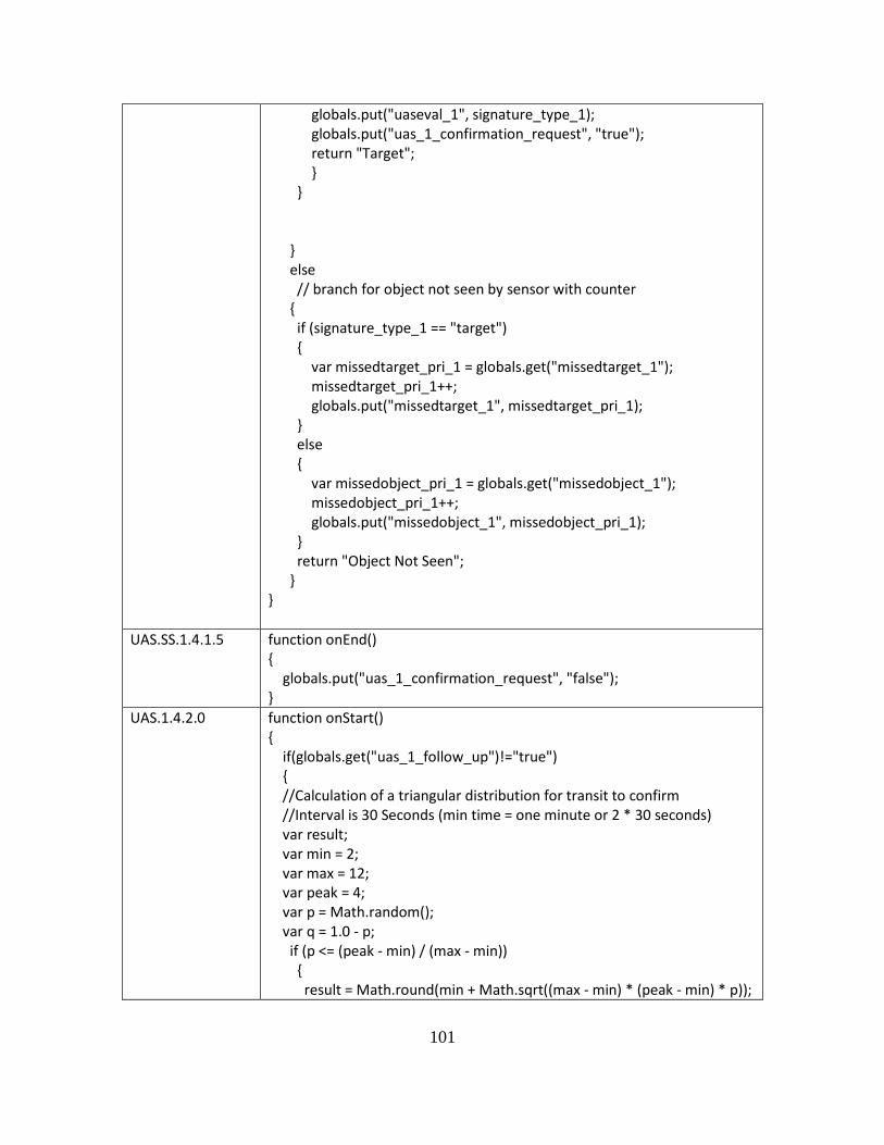
101
globals.put("uaseval_1", signature_type_1); globals.put("uas_1_confirmation_request", "true"); return "Target"; } } } else // branch for object not seen by sensor with counter { if (signature_type_1 == "target") { var missedtarget_pri_1 = globals.get("missedtarget_1"); missedtarget_pri_1++; globals.put("missedtarget_1", missedtarget_pri_1); } else { var missedobject_pri_1 = globals.get("missedobject_1"); missedobject_pri_1++; globals.put("missedobject_1", missedobject_pri_1); } return "Object Not Seen"; } }
UAS.SS.1.4.1.5 function onEnd() { globals.put("uas_1_confirmation_request", "false"); }
UAS.1.4.2.0 function onStart() { if(globals.get("uas_1_follow_up")!="true") { //Calculation of a triangular distribution for transit to confirm //Interval is 30 Seconds (min time = one minute or 2 * 30 seconds) var result; var min = 2; var max = 12; var peak = 4; var p = Math.random(); var q = 1.0 - p; if (p <= (peak - min) / (max - min)) { result = Math.round(min + Math.sqrt((max - min) * (peak - min) * p));

102
} else { result = Math.round(max - Math.sqrt((max - min) * (max - peak) * q)); } globals.put("transit_1", result); globals.put("transit_1_save", result); } globals.put("transit_1_count",0); } function onEnd() { var transit_1_req = globals.get("transit_1"); var transit_1_count = globals.get("transit_1_count"); transit_1_count++; globals.put("transit_1_count", transit_1_count); if(transit_1_count >= transit_1_req) { globals.put("transit_1_count",0); globals.put("uas_1_follow_up", "false") return false; } else { return true; } }
UAS.1.4.2.1 function onEnd() { //Retrieve object type var eval_type_1 = globals.get("uaseval_2"); //initialize variable for confusion matrix path var eval_confusion_1 = Math.random(); var truepositive = globals.get("truepositive"); var truenegative = globals.get("truenegative"); //Case of Target if(eval_type_1=="target")
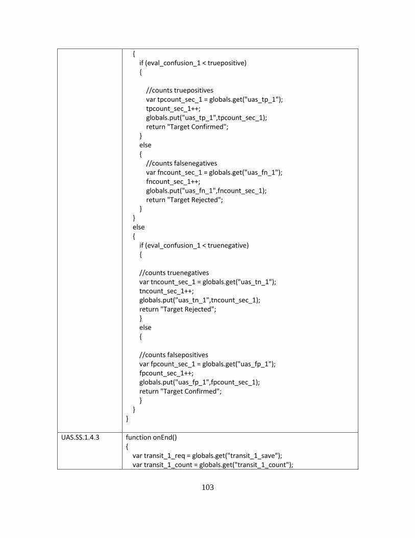
103
{ if (eval_confusion_1 < truepositive) { //counts truepositives var tpcount_sec_1 = globals.get("uas_tp_1"); tpcount_sec_1++; globals.put("uas_tp_1",tpcount_sec_1); return "Target Confirmed"; } else { //counts falsenegatives var fncount_sec_1 = globals.get("uas_fn_1"); fncount_sec_1++; globals.put("uas_fn_1",fncount_sec_1); return "Target Rejected"; } } else { if (eval_confusion_1 < truenegative) { //counts truenegatives var tncount_sec_1 = globals.get("uas_tn_1"); tncount_sec_1++; globals.put("uas_tn_1",tncount_sec_1); return "Target Rejected"; } else { //counts falsepositives var fpcount_sec_1 = globals.get("uas_fp_1"); fpcount_sec_1++; globals.put("uas_fp_1",fpcount_sec_1); return "Target Confirmed"; } } }
UAS.SS.1.4.3 function onEnd() { var transit_1_req = globals.get("transit_1_save"); var transit_1_count = globals.get("transit_1_count");

104
transit_1_count++; globals.put("transit_1_count", transit_1_count); if(globals.get("uas_2_confirmation_request")=="true") { globals.put("uas_1_follow_up", "true"); globals.put("transit_1", transit_1_count); return false; } if(transit_1_count >= transit_1_req) { return false; } else { return true; } }
MC.0 function onStart() { //intialize global mission status globals.put("missionstatus",0); //initialize launch duration value for UAS //Calculation of a triangular distribution for mission length var result; var min = 1; var max = 15; var peak = 5; var p = Math.random(); var q = 1.0 - p; if (p <= (peak - min) / (max - min)) { result = Math.round(min + Math.sqrt((max - min) * (peak - min) * p)); } else { result = Math.round(max - Math.sqrt((max - min) * (max - peak) * q)); } globals.put("launchfuel_1",result); globals.put("launchfuel_2",result);
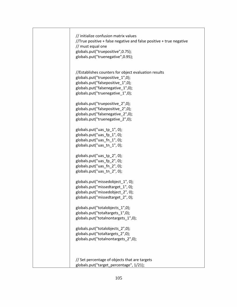
105
// initialize confusion matrix values //True positive + false negative and false positive + true negative // must equal one globals.put("truepositive",0.75); globals.put("truenegative",0.95); //Establishes counters for object evaluation results globals.put("truepositive_1",0); globals.put("falsepositive_1",0); globals.put("falsenegative_1",0); globals.put("truenegative_1",0); globals.put("truepositive_2",0); globals.put("falsepositive_2",0); globals.put("falsenegative_2",0); globals.put("truenegative_2",0); globals.put("uas_tp_1", 0); globals.put("uas_fp_1", 0); globals.put("uas_fn_1", 0); globals.put("uas_tn_1", 0); globals.put("uas_tp_2", 0); globals.put("uas_fp_2", 0); globals.put("uas_fn_2", 0); globals.put("uas_tn_2", 0); globals.put("missedobject_1", 0); globals.put("missedtarget_1", 0); globals.put("missedobject_2", 0); globals.put("missedtarget_2", 0); globals.put("totalobjects_1",0); globals.put("totaltargets_1",0); globals.put("totalnontargets_1",0); globals.put("totalobjects_2",0); globals.put("totaltargets_2",0); globals.put("totalnontargets_2",0); // Set percentage of objects that are targets globals.put("target_percentage", 1/21);

106
// Set percentage of objects that are seen by the sensor globals.put("detection_percentage", 0.85); globals.put("uas_1_confirmation_request", 0); globals.put("uas_2_confirmation_request", 0); }
MC.1 function onEnd() { // Mission control loop only exits upon mission status set to // recovery if(globals.get("missionstatus_1") == "recovery" || globals.get("missionstatus_2") == "recovery" ) { return false; } else { return true; } }
D.1 function onEnd() { print('1 Total Objects Emitted: ' + globals.get("totalobjects_1")); print('1 Total Targets Emitted: ' + globals.get("totaltargets_1")); print('1 Total Non-Targets Emitted: ' + globals.get("totalnontargets_1")); print('2 Total Objects Emitted: ' + globals.get("totalobjects_2")); print('2 Total Targets Emitted: ' + globals.get("totaltargets_2")); print('2 Total Non-Targets Emitted: ' + globals.get("totalnontargets_2")); print('1 Detected True Positives: ' + globals.get("truepositive_1")); print('1 Detected False Positives: ' + globals.get("falsepositive_1")); print('1 Detected True Negatives: ' + globals.get("truenegative_1")); print('1 Detected False Negatives: ' + globals.get("falsenegative_1")); print('1 Total Eligible Missed Non-targets: ' + globals.get("missedobject_1")); print('1 Total Eligible Missed Targets: ' + globals.get("missedtarget_1")); print('2 Detected True Positives: ' + globals.get("truepositive_2")); print('2 Detected False Positives: ' + globals.get("falsepositive_2")); print('2 Detected True Negatives: ' + globals.get("truenegative_2"));

107
print('2 Detected False Negatives: ' + globals.get("falsenegative_2")); print('2 Total Eligible Missed Non-targets: ' + globals.get("missedobject_2")); print('2 Total Eligible Missed Targets: ' + globals.get("missedtarget_2")); print('1 Confirmed True Positives: ' + globals.get("uas_tp_1")); print('1 Confirmed False Positives: ' + globals.get("uas_fp_1")); print('1 Confirmed True Negatives: ' + globals.get("uas_tn_1")); print('1 Confirmed False Negatives: ' + globals.get("uas_fn_1")); print('2 Confirmed True Positives: ' + globals.get("uas_tp_2")); print('2 Confirmed False Positives: ' + globals.get("uas_fp_2")); print('2 Confirmed True Negatives: ' + globals.get("uas_tn_2")); print('2 Confirmed False Negatives: ' + globals.get("uas_fn_2")); var launchduration = globals.get("launchfuel_1"); var missionduration = 60 - 2*launchduration; print('Total Mission Duration in Minutes: ' +missionduration); }

108
Acronyms
ABEP Architecture Based Evaluation Process
AoA Analysis of Alternatives
ATR Autonomous Target Recognition
COCOM Combatant Commander
CONOPS Concept of Operations
CPN Colored Petri-Net
DES Discrete Event Simulation
DoD Department of Defense
DoDAF Department of Defense Architecture Framework
EA Executable Architecture
EFFBD Enhanced Function Flow Block Diagram
FFBD Function Flow Block Diagram
GCS Ground Control Station
HCPN Hierarchical Colored Petri-Net
ISR Intelligence, Surveillance and Reconnaissance
MOE Measure of Effectiveness
MP Monterey Phoenix
SE Systems Engineering
SoS System of Systems
SysML Systems Modeling Language
UAS Unmanned Aerial System
UML Unified Modeling Language

109
Bibliography
Auguston, M. (2014). Behavior Models for Software Architecture. Retrieved from
http://www.dtic.mil/dtic/tr/fulltext/u2/a611836.pdf
Bienvenu, M. P., Shin, I., & Levis, A. H. (2000). C4ISR architectures: III. An object-
oriented approach for architecture design. Systems Engineering, 3(4), 288–312.
http://doi.org/10.1002/1520-6858(2000)3:4<288::AID-SYS6>3.0.CO;2-F
Cancro, G., Turner, R., Kahn, E., & Williams, S. (2011, January). Executable
specification-based system engineering. Aerospace Conference, 2011 IEEE.
Retrieved from
http://ieeexplore.ieee.org/xpl/articleDetails.jsp?tp=&arnumber=5747626&contentTy
pe=Conference+Publications
Defense Acquisition University. (2014). Generic Acquisition Process (Pre-Tailoring),
5000. Retrieved from https://dap.dau.mil/aphome/Documents/Defense Acquisition
Waterfall Chart with color enhancements 17 Dec final (3).pdf
Department of Defense. (2007a). DoD Architecture Framework Volume I : Definitions
and Guidelines. Architecture, I(April 2007), 1–46.
Department of Defense. (2007b). DoD Architecture Framework Volume II : Product
Descriptions. Architecture, II(April 2007), 284.
110
Dietrichs, T., Griffin, R., Schuettke, A., & Slocum, M. (2006). INTEGRATED
ARCHITECTURE STUDY FOR WEAPON BORNE BATTLE DAMAGE
ASSESSMENT SYSTEM EVALUATION. Air Force Institute of Technology, Air
University.
DoD Deputy Chief Information Officer. (2009). The DoDAF Architecture Framework
Version 2.0. U.S. Department of Defense. Retrieved from http://cio-
nii.defense.gov/sites/dodaf20/index.html
Feng, N., Ming-Zhe, W., Cui-Rong, Y., & Zhi-Gang, T. (2010, January). Executable
architecture modeling and validation. Computer and Automation Engineering
(ICCAE), 2010 The 2nd International Conference on. Retrieved from
http://ieeexplore.ieee.org/xpl/articleDetails.jsp?tp=&arnumber=5452010&contentTy
pe=Conference+Publications
Ge, B., Hipel, K. W., Li, L., & Chen, Y. (2012, January). A data-centric executable
modeling approach for system-of-systems architecture. System of Systems
Engineering (SoSE), 2012 7th International Conference on.
Ge, B., Hipel, K. W., Yang, K., & Chen, Y. (2014, January). A Novel Executable
Modeling Approach for System-of-Systems Architecture. Systems Journal, IEEE.
Retrieved from
http://ieeexplore.ieee.org/xpl/articleDetails.jsp?tp=&arnumber=6565359&contentTy
pe=Journals+&+Magazines

111
Griendling, K., & Mavris, D. N. (2011, January). Development of a dodaf-based
executable architecting approach to analyze system-of-systems alternatives.
Aerospace Conference, 2011 IEEE. Retrieved from
http://ieeexplore.ieee.org/xpl/articleDetails.jsp?tp=&arnumber=5747654&contentTy
pe=Conference+Publications
Hu, J., Huang, L., Cao, B., & Chang, X. (2014). SPDML: Graphical modeling language
for executable architecture of systems. 6th International Conference on Cyber-
Enabled Distributed Computing and Knowledge Discovery, CyberC 2014, 248–255.
http://doi.org/10.1109/CyberC.2014.52
IEEE Standard 1220-2005. (2007). IEEE Standard for Application and Management of
the Systems Engineering Process.
Imagine That! (2015). ExtendSim Simulation Software. Retrieved September 9, 2015,
from https://www.extendsim.com/
Intercax. (2015a). ParaMagic® plugin for MagicDraw - Intercax. Retrieved December 9,
2015, from http://intercax.com/products/paramagic/
Intercax. (2015b). SolveaTM - SysML Parametric Solver - Intercax. Retrieved December
9, 2015, from http://intercax.com/products/solvea/
Janczura, C. (2009). Evaluation of Defence Architectures in Support of System
Integration. Journal of Battlefield Technology, 12(3), 9 – 13. Retrieved from

112
http://ezproxy.library.capella.edu/login?url=http://search.ebscohost.com.library.cape
lla.edu/login.aspx?direct=true&db=tsh&AN=44639406&site=ehost-live&scope=site
Jensen, K., Kristensen, L., & Wells, L. (2007, January). Coloured Petri Nets and CPN
Tools for modelling and validation of concurrent systems. International Journal on
Software Tools for Technology Transfer. Retrieved from
http://search.ebscohost.com/login.aspx?direct=true&db=a9h&AN=25234751&site=
ehost-live
Larman, C. (2011). Applying UML and Patterns. (D. O’Hagan, J. Fuller, & J. Nahil,
Eds.) (14th ed.). Upper Saddle River, NJ: Prentice Hall.
Levis, A. H., & Wagenhals, L. W. (2000). C4ISR architectures: I. Developing a process
for C4ISR architecture design. Systems Engineering, 3(4), 225–247.
http://doi.org/10.1002/1520-6858(2000)3:4<225::AID-SYS4>3.0.CO;2-#
Li, L., Dou, Y., Ge, B., Yang, K., & Chen, Y. (2012). Executable System-of-Systems
architecting based on DoDAF meta-model. System of Systems Engineering (SoSE),
2012 7th International Conference on, 362–367.
http://doi.org/10.1109/SYSoSE.2012.6384204
Mathworks. (2015). Discrete Event Simulation Software - SimEvents. Retrieved
September 9, 2015, from http://www.mathworks.com/products/simevents/

113
Matloff, N. S. (2008). Introduction to discrete-event simulation and the simpy language.
Davis, CA. Dept of Computer Science. University, 1–33. Retrieved from
http://heather.cs.ucdavis.edu/~matloff/156/PLN/DESimIntro.pdf
Nakhla, N. M., & Wheaton, K. (2014). An executable architecture tool for the modeling
and simulation of operational process models. 8th Annual IEEE International
Systems Conference, SysCon 2014 - Proceedings, 489–496.
http://doi.org/10.1109/SysCon.2014.6819301
No Magic. (2015). Cameo Simulation Toolkt.
Özgün, O., & Barlas, Y. (2009). Discrete vs . Continuous Simulation : When Does It
Matter ? 27th International Conference of The System Dynamics Society, (06), 1–22.
Rockwell Automation. (2015). Arena Discrete Event Simulation Software. Retrieved
September 9, 2015, from https://www.arenasimulation.com/
Sparx Systems. (2015). How it Works [Enterprise Architect User Guide]. Retrieved
January 1, 2015, from
http://www.sparxsystems.com/enterprise_architect_user_guide/9.2/model_simulatio
n/how_it_works2.html
SPEC Innovations. (2015). DoDAF Software Tools | Innoslate. Retrieved January 1,
2015, from https://www.innoslate.com/dodaf/
114
Staines, T. S. (2008, January). Intuitive Mapping of UML 2 Activity Diagrams into
Fundamental Modeling Concept Petri Net Diagrams and Colored Petri Nets.
Engineering of Computer Based Systems, 2008.ECBS 2008.15th Annual IEEE
International Conference and Workshop on the. Retrieved from
http://ieeexplore.ieee.org/xpl/articleDetails.jsp?tp=&arnumber=4492400&contentTy
pe=Conference+Publications
The Object Management Group. (2012). Semantics of a Foundational Subset for
Executable UML Models (fUML), (October), 441. Retrieved from
http://www.omg.org/spec/FUML/
Vitech Corporation. (2000). COREsim User Guide 3.0.
Wagenhals, L. W., & Levis, A. H. (2009, January). Service Oriented Architectures, the
DoD Architecture Framework 1.5, and Executable Architectures. SYSTEMS
ENGINEERING. Retrieved from
http://gateway.webofknowledge.com/gateway/Gateway.cgi?&GWVersion=2&SrcA
uth=SerialsSolutions&SrcApp=360&DestLinkType=FullRecord&DestApp=WOS&
KeyUT=WOS:000271966700003
Wagenhals, L. W., Liles, S. W., & Levis, A. H. (2009, January). Toward executable
architectures to support evaluation. Collaborative Technologies and Systems,
2009.CTS ’09.International Symposium on. Retrieved from
http://ieeexplore.ieee.org/xpl/articleDetails.jsp?tp=&arnumber=5067520&contentTy
pe=Conference+Publications

115
Wagenhals, L. W., Shin, I., Kim, D., & Levis, A. H. (2000). C4ISR Architectures: II. A
Structured Analysis Approach for Architecture Design. Systems Engineering, 3(4),
248–287.
Wang, Z., He, H., & Wang, Q. (2014). Executable Architecture Modeling and Simulation
Based on fUML. In 19th International Command and Control Research and
Technology Symposium (pp. 1–17). Alexandria, VA.
Xia, X., Wu, J., Liu, C., & Xu, L. (2013). A Model-Driven Approach for Evaluating
System of Systems. Engineering of Complex Computer Systems (ICECCS), 2013
18th International Conference on. Retrieved from
http://ieeexplore.ieee.org/xpl/articleDetails.jsp?tp=&arnumber=6601805&contentTy
pe=Conference+Publications

116
REPORT DOCUMENTATION PAGE Form Approved OMB No. 074-0188
The public reporting burden for this collection of information is estimated to average 1 hour per response, including the time for reviewing instructions, searching existing data sources, gathering and maintaining the data needed, and completing and reviewing the collection of information. Send comments regarding this burden estimate or any other aspect of the collection of information, including suggestions for reducing this burden to Department of Defense, Washington Headquarters Services, Directorate for Information Operations and Reports (0704-0188), 1215 Jefferson Davis Highway, Suite 1204, Arlington, VA 22202-4302. Respondents should be aware that notwithstanding any other provision of law, no person shall be subject to an penalty for failing to comply with a collection of information if it does not display a currently valid OMB control number. PLEASE DO NOT RETURN YOUR FORM TO THE ABOVE ADDRESS. 1. REPORT DATE (DD-MM-YYYY)
24-12-2015 2. REPORT TYPE
Master’s Thesis 3. DATES COVERED (From – To)
October 2014 – December 2015
TITLE AND SUBTITLE Application of Executable Architectures in Early Concept Evaluation
5a. CONTRACT NUMBER
5b. GRANT NUMBER 5c. PROGRAM ELEMENT NUMBER
6. AUTHOR(S) Pospisal, Ryan M., Major, USAF
5d. PROJECT NUMBER
5e. TASK NUMBER
5f. WORK UNIT NUMBER
7. PERFORMING ORGANIZATION NAMES(S) AND ADDRESS(S) Air Force Institute of Technology Graduate School of Engineering and Management (AFIT/EN) 2950 Hobson Way, Building 640 WPAFB OH 45433-7765
8. PERFORMING ORGANIZATION REPORT NUMBER AFIT-ENV-MS-15-D-027
9. SPONSORING/MONITORING AGENCY NAME(S) AND ADDRESS(ES) DoD Systems Engineering Research Center Scott Lucero, Deputy Director, Strategic Initiatives, ODASD(SE) 1 Castle Point Terrace Hoboken, NJ 07030 [email protected] (703) 681-6654
10. SPONSOR/MONITOR’S ACRONYM(S) ODASD(SE) 11. SPONSOR/MONITOR’S REPORT NUMBER(S)
12. DISTRIBUTION/AVAILABILITY STATEMENT DISTRUBTION STATEMENT A. APPROVED FOR PUBLIC RELEASE; DISTRIBUTION UNLIMITED.
13. SUPPLEMENTARY NOTES This material is declared a work of the U.S. Government and is not subject to copyright protection in the United States. 14. ABSTRACT This research explores use of executable architectures to guide design decisions in the early stages of system development. Decisions made early in the system development cycle determine a majority of the total lifecycle costs as well as establish a baseline for long term system performance and thus it is vital to program success to choose favorable design alternatives. The development of a representative architecture followed the Architecture Based Evaluation Process as it provides a logical and systematic order of events to produce an architecture sufficient to document and model operational performance. In order to demonstrate the value in the application of executable architectures for trade space decisions, three variants of a fictional unmanned aerial system were developed and simulated. Four measures of effectiveness (MOEs) were selected for evaluation. Two parameters of interest were varied at two levels during simulation to create four test case scenarios against which to evaluate each variant. Analysis of the resulting simulation demonstrated the ability to obtain a statistically significant difference in MOE performance for 10 out of 16 possible test case-MOE combinations. Additionally, for the given scenarios, the research demonstrated the ability to make a conclusive selection of the superior variant for additional development. 15. SUBJECT TERMS Executable Architecture, DoDAF, Analysis of Alternatives, AoA, System of Systems, SoS 16. SECURITY CLASSIFICATION OF:
17. LIMITATION OF ABSTRACT
UU
18. NUMBER OF PAGES
129
19a. NAME OF RESPONSIBLE PERSON Dr. David Jacques, AFIT/ENV
a. REPORT
U
b. ABSTRACT
U
c. THIS PAGE
U
19b. TELEPHONE NUMBER (Include area code) (937) 255-3355, ext 3329 ([email protected])
Standard Form 298 (Rev. 8-98) Prescribed by ANSI Std. Z39-18