Application ofEuler and Homotopy Operators

to Integrability Testing

Willy HeremanDepartment of Applied Mathematics and Statistics

Colorado School of Mines

Golden, Colorado, U.S.A.

http://www.mines.edu/fs home/whereman/

The Ninth IMACS International Conference on

Nonlinear Evolution Equations and Wave Phenomena:

Computation and Theory

Athens, Georgia

Thursday, April 2, 2015, 4:40p.m.

Acknowledgements

Douglas Poole (Chadron State College, Nebraska)

Unal Goktas (Turgut Ozal University, Turkey)

Mark Hickman (Univ. of Canterbury, New Zealand)

Bernard Deconinck (Univ. of Washington, Seattle)

Several undergraduate and graduate students

Research supported in part by NSF

under Grant No. CCF-0830783

This presentation was made in TeXpower

Outline

• Motivation of the Research

• Part I: Continuous Case

I Calculus-based formulas for the continuous

homotopy operator (in multi-dimensions)

See: Anco & Bluman (2002); Hereman et al.

(2007); Olver (1986)

I Symbolic integration by parts and inversion

of the total divergence operator

I Application: symbolic computation of

conservation laws of nonlinear PDEs in

multiple space dimensions

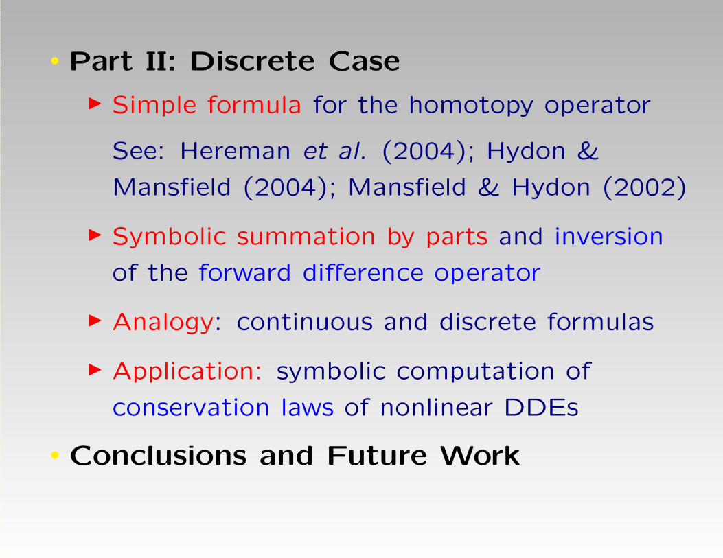
• Part II: Discrete Case

I Simple formula for the homotopy operator

See: Hereman et al. (2004); Hydon &

Mansfield (2004); Mansfield & Hydon (2002)

I Symbolic summation by parts and inversion

of the forward difference operator

I Analogy: continuous and discrete formulas

I Application: symbolic computation of

conservation laws of nonlinear DDEs

• Conclusions and Future Work

Motivation of the Research

Conservation Laws for Nonlinear PDEs

• System of evolution equations of order M

ut = F(u(M)(x))

with u = (u, v, w, . . .) and x = (x, y, z).

• Conservation law in (1+1)-dimensions

Dtρ+ DxJ = 0

where = means evaluated on the PDE.

Conserved density ρ and flux J.

• Conservation law in (2+1)-dimensions

Dtρ+∇·J = Dtρ+ DxJ1 + DyJ2 = 0

Conserved density ρ and flux J = (J1, J2).

• Conservation law in (3+1)-dimensions

Dtρ+∇·J = Dtρ+ DxJ1 + DyJ2 + DzJ3 = 0

Conserved density ρ and flux J = (J1, J2, J3).

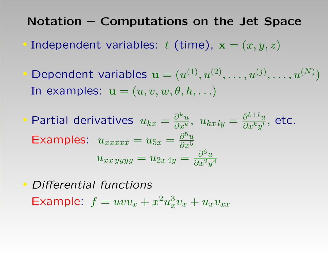
Notation – Computations on the Jet Space

• Independent variables: t (time), x = (x, y, z)

• Dependent variables u = (u(1), u(2), . . . , u(j), . . . , u(N))

In examples: u = (u, v, w, θ, h, . . .)

• Partial derivatives ukx = ∂ku∂xk

, ukx ly = ∂k+lu∂xkyl

, etc.

Examples: uxxxxx = u5x = ∂5u∂x5

uxx yyyy = u2x 4y = ∂6u∂x2y4

• Differential functions

Example: f = uvvx + x2u3xvx + uxvxx

• Total derivatives: Dt, Dx,Dy, . . .

Example: Let f = uvvx + x2u3xvx + uxvxx Then

Dxf =∂f

∂x+ ux

∂f

∂u+ uxx

∂f

∂ux

+vx∂f

∂v+ vxx

∂f

∂vx+ vxxx

∂f

∂vxx

= 2xu3xvx + ux(vvx) + uxx(3x

2u2xvx + vxx)

+vx(uvx) + vxx(uv + x2u3x) + vxxx(ux)

= 2xu3xvx + vuxvx + 3x2u2

xvxuxx + uxxvxx

+uv2x + uvvxx + x2u3

xvxx + uxvxxx

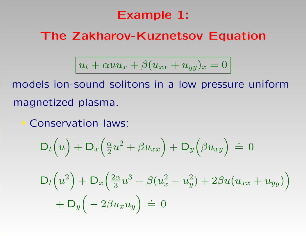
Example 1:

The Zakharov-Kuznetsov Equation

ut + αuux + β(uxx + uyy)x = 0

models ion-sound solitons in a low pressure uniform

magnetized plasma.

• Conservation laws:

Dt

(u)

+ Dx

(α2u2 + βuxx

)+ Dy

(βuxy

)= 0

Dt

(u2)

+ Dx

(2α3u3 − β(u2

x − u2y) + 2βu(uxx + uyy)

)+ Dy

(− 2βuxuy

)= 0

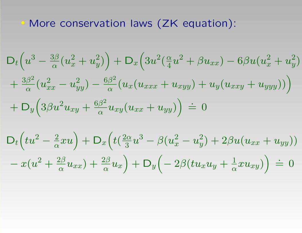
• More conservation laws (ZK equation):

Dt

(u3 − 3β

α(u2

x + u2y))

+ Dx

(3u2(α

4u2 + βuxx)− 6βu(u2

x + u2y)

+ 3β2

α(u2

xx − u2yy)−

6β2

α(ux(uxxx + uxyy) + uy(uxxy + uyyy))

)+ Dy

(3βu2uxy + 6β2

αuxy(uxx + uyy)

)= 0

Dt

(tu2 − 2

αxu)

+ Dx

(t(2α

3u3 − β(u2

x − u2y) + 2βu(uxx + uyy))

− x(u2 + 2βαuxx) + 2β

αux)

+ Dy

(− 2β(tuxuy + 1

αxuxy)

)= 0

Example 2:

Shallow Water Wave Equations

P. Dellar, Phys. Fluids 15 (2003) 292-297

ut + (u·∇)u + 2 Ω× u +∇(θh)− 12h∇θ = 0

θt + u·(∇θ) = 0

ht +∇·(uh) = 0

In components:ut + uux + vuy − 2 Ωv + 1

2hθx + θhx = 0

vt + uvx + vvy + 2 Ωu+ 12hθy + θhy = 0

θt + uθx + vθy = 0

ht + hux + uhx + hvy + vhy = 0

where u(x, y, t), θ(x, y, t) and h(x, y, t)

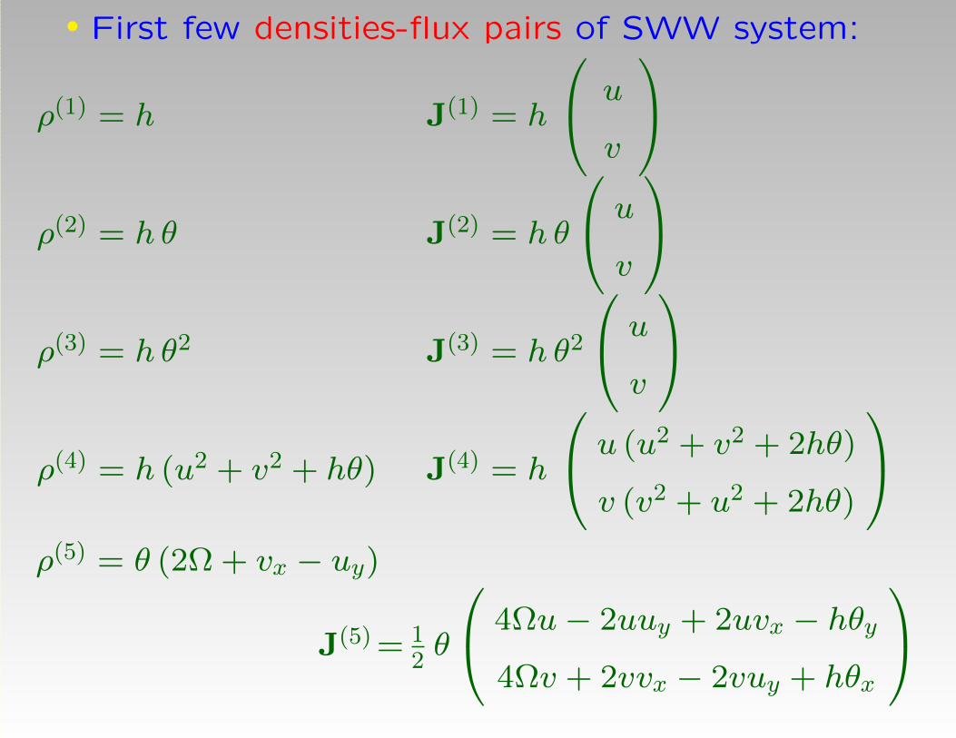
• First few densities-flux pairs of SWW system:

ρ(1) = h J(1) = h

u

v

ρ(2) = h θ J(2) = h θ

u

v

ρ(3) = h θ2 J(3) = h θ2

u

v

ρ(4) = h (u2 + v2 + hθ) J(4) = h

u (u2 + v2 + 2hθ)

v (v2 + u2 + 2hθ)

ρ(5) = θ (2Ω + vx − uy)

J(5) = 12θ

4Ωu− 2uuy + 2uvx − hθy4Ωv + 2vvx − 2vuy + hθx

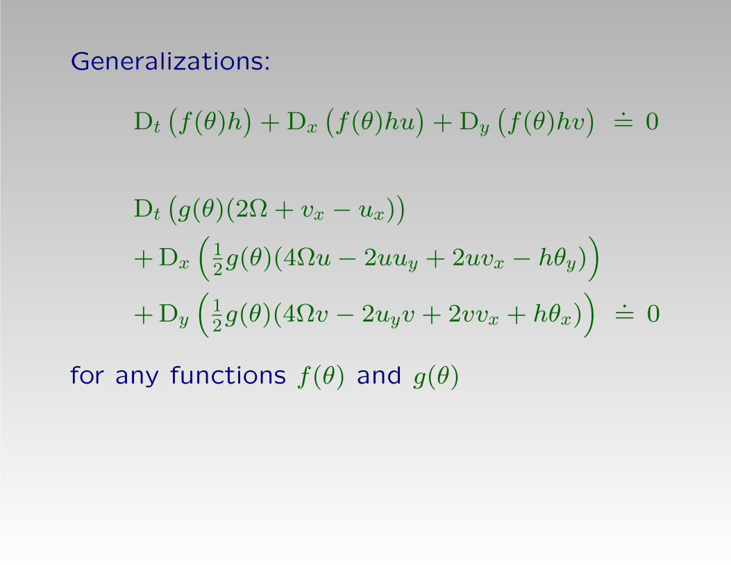
Generalizations:

Dt

(f(θ)h

)+ Dx

(f(θ)hu

)+ Dy

(f(θ)hv

)= 0

Dt

(g(θ)(2Ω + vx − ux)

)+ Dx

(12g(θ)(4Ωu− 2uuy + 2uvx − hθy)

)+ Dy

(12g(θ)(4Ωv − 2uyv + 2vvx + hθx)

)= 0

for any functions f(θ) and g(θ)

Conservation Laws for Nonlinear

Differential-Difference Equations (DDEs)

• System of DDEs

un=F(· · · ,un−1,un,un+1, · · · )

• Conservation law in (1 + 1) dimensions

Dtρn + ∆Jn = Dtρn + Jn+1 − Jn = 0

conserved density ρn and flux Jn

• Example: Toda lattice

un = vn−1 − vnvn = vn(un − un+1)

• First few densities-flux pairs for Toda lattice:

ρ(0)n =ln(vn) J

(0)n =un

ρ(1)n =un J

(1)n =vn−1

ρ(2)n = 1

2u2n + vn J

(2)n =unvn−1

ρ(3)n = 1

3u3n + un(vn−1 + vn) J

(3)n =un−1unvn−1 + v2

n−1

PART I: CONTINUOUS CASE

Problem Statement

Continuous case in 1D:

Example: For u(x) and v(x)

f=8vxvxx −u3x sinu+2uxuxx cosu−6vvx cosu+3uxv

2 sinu

Question: Can the expression be integrated?

If yes, find F =

∫f dx (so, f = DxF )

Result (by hand): F = 4 v2x + u2

x cosu− 3 v2 cosu

Continuous case in 2D or 3D:

Example: For u(x, y) and v(x, y)

f = uxvy − u2xvy − uyvx + uxyvx

Question: Is there an F so that f = Div F ?

If yes, find F.

Result (by hand): F = (uvy − uxvy,−uvx + uxvx)

Can this be done without integration by parts?

Can the computation be reduced to a single integral

in one variable?

Tools from the Calculus of Variations

• Definition:

A differential function f is a exact iff f = Div F.

Special case (1D): f = Dx F.

• Question: How can one test that f = Div F ?

• Theorem (exactness test):

f = Div F iff Lu(j)(x) f ≡ 0, j = 1, 2, . . . , N.

N is the number of dependent variables.

The Euler operator annihilates divergences

• Euler operator in 1D (variable u(x)):

Lu(x) =M∑k=0

(−Dx)k ∂

∂ukx

=∂

∂u−Dx

∂

∂ux+ D2

x

∂

∂uxx−D3

x

∂

∂uxxx+ · · ·

• Euler operator in 2D (variable u(x, y)):

Lu(x,y) =

Mx∑k=0

My∑`=0

(−Dx)k(−Dy)

` ∂

∂ukx `y

=∂

∂u−Dx

∂

∂ux−Dy

∂

∂uy

+ D2x

∂

∂uxx+DxDy

∂

∂uxy+D2

y

∂

∂uyy−D3

x

∂

∂uxxx· · ·

Application: Testing Exactness – Continous Case

Example:

f=8vxvxx −u3x sinu+2uxuxx cosu−6vvx cosu+3uxv

2 sinu

where u(x) and v(x)

• f is exact

• After integration by parts (by hand):

F =

∫f dx = 4 v2

x + u2x cosu− 3 v2 cosu

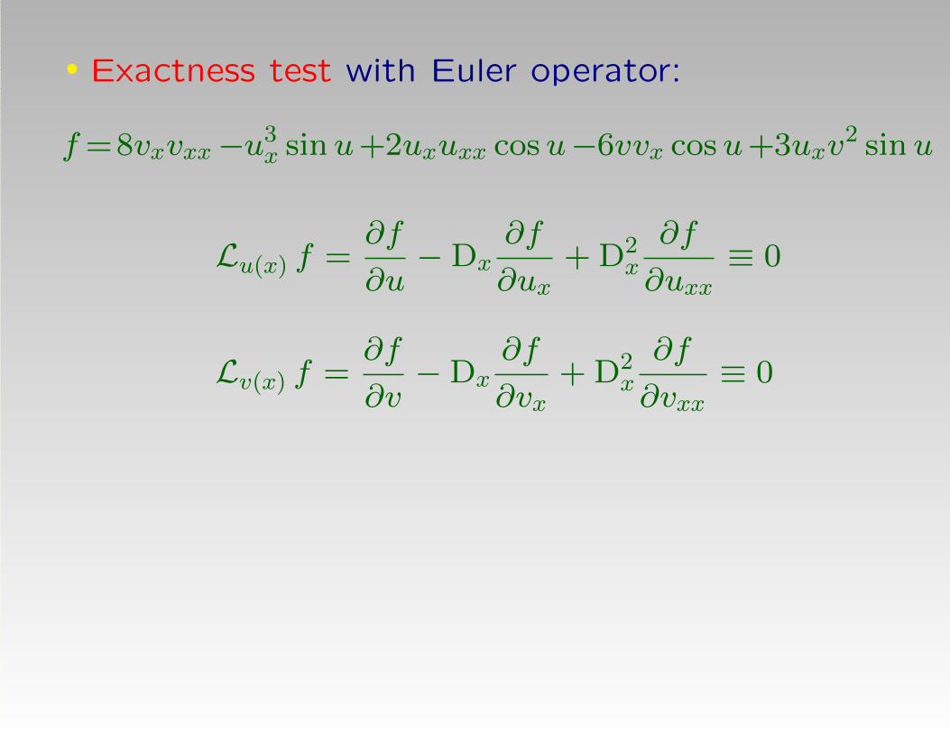
• Exactness test with Euler operator:

f=8vxvxx−u3x sinu+2uxuxx cosu−6vvx cosu+3uxv

2 sinu

Lu(x) f =∂f

∂u−Dx

∂f

∂ux+ D2

x

∂f

∂uxx≡ 0

Lv(x) f =∂f

∂v−Dx

∂f

∂vx+ D2

x

∂f

∂vxx≡ 0

• Question: How can one compute F = Div−1 f ?

• Theorem (integration by parts):

• In 1D: If f is exact then

F = D−1x f =

∫f dx = Hu(x)f

• In 2D: If f is a divergence then

F = Div−1 f = (H(x)u(x,y)f, H

(y)u(x,y)f)

The homotopy operator inverts total

derivatives and divergences!

Peter Olver’s Book

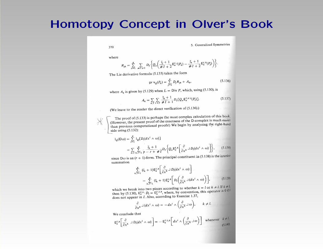
Homotopy Concept in Olver’s Book

Homotopy Formula in Olver’s Book

Zoom into Homotopy Formula in Olver’s Book

• Homotopy Operator in 1D (variable x):

Hu(x)f =

∫ 1

0

N∑j=1

(Iu(j)f)[λu]dλ

λ

with integrand

Iu(j)f =

M(j)x∑

k=1

k−1∑i=0

u(j)ix (−Dx)k−(i+1)

∂f

∂u(j)kx

(Iu(j)f)[λu] means that in Iu(j)f one replaces

u→ λu, ux → λux, etc.

More general: u→ λ(u− u0) + u0

ux → λ(ux − ux0) + ux0 etc.

• Homotopy Operator in 2D (variables x and y):

H(x)u(x,y) f =

∫ 1

0

N∑j=1

(I(x)

u(j)f)[λu]

dλ

λ

H(y)u(x,y) f =

∫ 1

0

N∑j=1

(I(y)

u(j)f)[λu]

dλ

λ

where for dependent variable u(x, y)

I(x)u f =

Mx∑k=1

My∑`=0

k−1∑i=0

∑j=0

uix jy

(i+ji

)(k+`−i−j−1k−i−1

)(k+`k

)(−Dx)

k−i−1 (−Dy

)`−j) ∂f

∂ukx `y

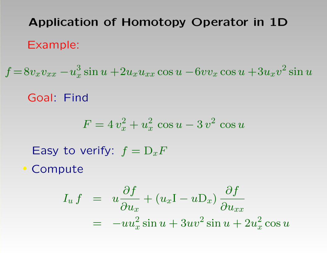
Application of Homotopy Operator in 1D

Example:

f=8vxvxx −u3x sinu+2uxuxx cosu−6vvx cosu+3uxv

2 sinu

Goal: Find

F = 4 v2x + u2

x cosu− 3 v2 cosu

Easy to verify: f = DxF

• Compute

Iu f = u∂f

∂ux+ (uxI− uDx)

∂f

∂uxx

= −uu2x sinu+ 3uv2 sinu+ 2u2

x cosu

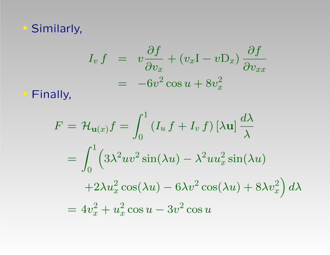
• Similarly,

Iv f = v∂f

∂vx+ (vxI− vDx)

∂f

∂vxx

= −6v2 cosu+ 8v2x

• Finally,

F = Hu(x)f =

∫ 1

0(Iu f + Iv f) [λu]

dλ

λ

=

∫ 1

0

(3λ2uv2 sin(λu)− λ2uu2

x sin(λu)

+2λu2x cos(λu)− 6λv2 cos(λu) + 8λv2

x

)dλ

= 4v2x + u2

x cosu− 3v2 cosu

Application of Homotopy Operator in 2D

• Example: f = uxvy − uxxvy − uyvx + uxyvx

By hand: F = (uvy − uxvy,−uvx + uxvx)

Easy to verify: f = Div F

• Compute

I(x)u f = u

∂f

∂ux+ (uxI− uDx)

∂f

∂uxx

+(

12uyI− 1

2uDy

) ∂f

∂uxy

= uvy + 12uyvx − uxvy + 1

2uvxy

• Similarly,

I(x)v f = v

∂f

∂vx= −uyv + uxyv

• Hence,

F1 = H(x)u(x,y)f=

∫ 1

0

(I(x)u f + I(x)

v f)

[λu]dλ

λ

=

∫ 1

0λ(uvy + 1

2uyvx − uxvy + 1

2uvxy − uyv + uxyv

)dλ

= 12uvy + 1

4uyvx − 1

2uxvy + 1

4uvxy − 1

2uyv + 1

2uxyv

• Analogously,

F2 = H(y)u(x,y)f=

∫ 1

0

(I(y)u f + I(y)

v f)

[λu]dλ

λ

=

∫ 1

0

(λ(−uvx − 1

2uvxx + 1

2uxvx

)+ λ (uxv − uxxv)

)dλ

= −12uvx − 1

4uvxx + 1

4uxvx + 1

2uxv − 1

2uxxv

• So,

F=1

4

2uvy + uyvx − 2uxvy + uvxy − 2uyv + 2uxyv

−2uvx − uvxx + uxvx + 2uxv − 2uxxv

Let K= F−F then

K=1

4

2uvy − uyvx − 2uxvy − uvxy + 2uyv − 2uxyv

−2uvx + uvxx + 3uxvx − 2uxv + 2uxxv

then Div K = 0

• Also, K = (Dyφ,−Dxφ) with φ = 14(2uv − uvx − 2uxv)

(curl in 2D)

After removing the curl term K:

F = F + K = (uvy − uxvy,−uvx + uxvx)

Avoid curl terms algorithmically!

Why does this work?

Sketch of Derivation and Proof

(in 1D with variable x, and for one component u)

Definition: Degree operator M

Mf =M∑i=0

uix∂f

∂uix= u

∂f

∂u+ux

∂f

∂ux+u2x

∂f

∂u2x+· · ·+uMx

∂f

∂uMx

f is of order M in x

Example: f = upuqxur3x (p, q, r non-negative integers)

g =Mf =

3∑i=0

uix∂f

∂uix= (p+ q + r)upuqxu

r3x

Application of M computes the total degree

Theorem (inverse operator) M−1g(u) =∫ 1

0 g[λu] dλλ

Proof:

d

dλg[λu] =

M∑i=0

∂g[λu]

∂λuix

dλuix

dλ=

1

λ

M∑i=0

uix∂g[λu]

∂uix=

1

λMg[λu]

Integrate both sides with respect to λ∫ 1

0

d

dλg[λu] dλ = g[λu]

∣∣λ=1

λ=0= g(u)− g(0)

=

∫ 1

0Mg[λu]

dλ

λ=M

∫ 1

0g[λu]

dλ

λ

Assuming g(0) = 0,

M−1g(u) =

∫ 1

0g[λu]

dλ

λ

Example:

If g(u) = (p+ q + r)upuqxur3x, then

g[λu] = (p+ q + r)λp+q+r upuqxur3x

Hence,

M−1g =

∫ 1

0(p+ q + r)λp+q+r−1 upuqxu

r3x dλ

= upuqxur3x λ

p+q+r∣∣∣λ=1

λ=0= upuqxu

r3x

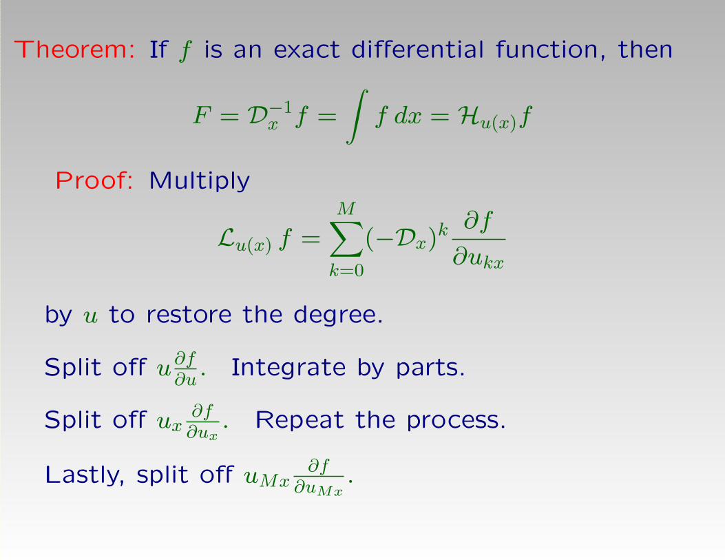
Theorem: If f is an exact differential function, then

F = D−1x f =

∫f dx = Hu(x)f

Proof: Multiply

Lu(x) f =

M∑k=0

(−Dx)k∂f

∂ukx

by u to restore the degree.

Split off u∂f∂u. Integrate by parts.

Split off ux∂f∂ux

. Repeat the process.

Lastly, split off uMx∂f

∂uMx.

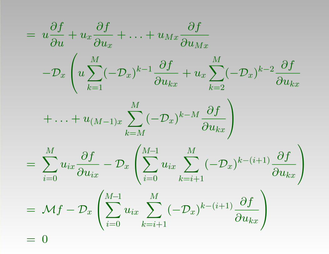
uLu(x)f = u

M∑k=0

(−Dx)k∂f

∂ukx

= u∂f

∂u−Dx

u M∑k=1

(−Dx)k−1 ∂f

∂ukx

+ ux

M∑k=1

(−Dx)k−1 ∂f

∂ukx

= u∂f

∂u+ ux

∂f

∂ux−Dx

u M∑k=1

(−Dx)k−1 ∂f

∂ukx

+ux

M∑k=2

(−Dx)k−2 ∂f

∂ukx

+ u2x

M∑k=2

(−Dx)k−2 ∂f

∂ukx

= . . .

= u∂f

∂u+ ux

∂f

∂ux+ . . .+ uMx

∂f

∂uMx

−Dx

u M∑k=1

(−Dx)k−1 ∂f

∂ukx+ ux

M∑k=2

(−Dx)k−2 ∂f

∂ukx

+ . . .+ u(M−1)x

M∑k=M

(−Dx)k−M∂f

∂ukx

=

M∑i=0

uix∂f

∂uix−Dx

M−1∑i=0

uix

M∑k=i+1

(−Dx)k−(i+1) ∂f

∂ukx

= Mf −Dx

M−1∑i=0

uix

M∑k=i+1

(−Dx)k−(i+1) ∂f

∂ukx

= 0

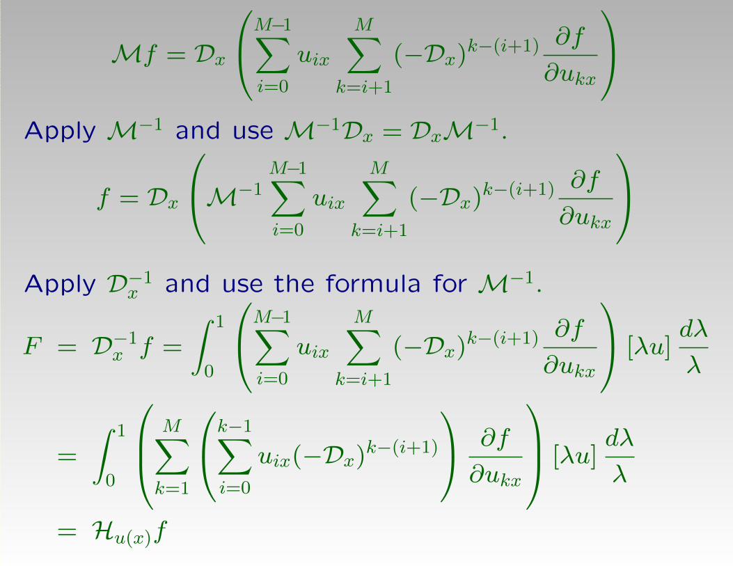
Mf = Dx

M−1∑i=0

uix

M∑k=i+1

(−Dx)k−(i+1) ∂f

∂ukx

Apply M−1 and use M−1Dx = DxM−1.

f = Dx

M−1M−1∑i=0

uix

M∑k=i+1

(−Dx)k−(i+1) ∂f

∂ukx

Apply D−1

x and use the formula for M−1.

F = D−1x f =

∫ 1

0

M−1∑i=0

uix

M∑k=i+1

(−Dx)k−(i+1) ∂f

∂ukx

[λu]dλ

λ

=

∫ 1

0

M∑k=1

k−1∑i=0

uix(−Dx)k−(i+1)

∂f

∂ukx

[λu]dλ

λ

= Hu(x)f

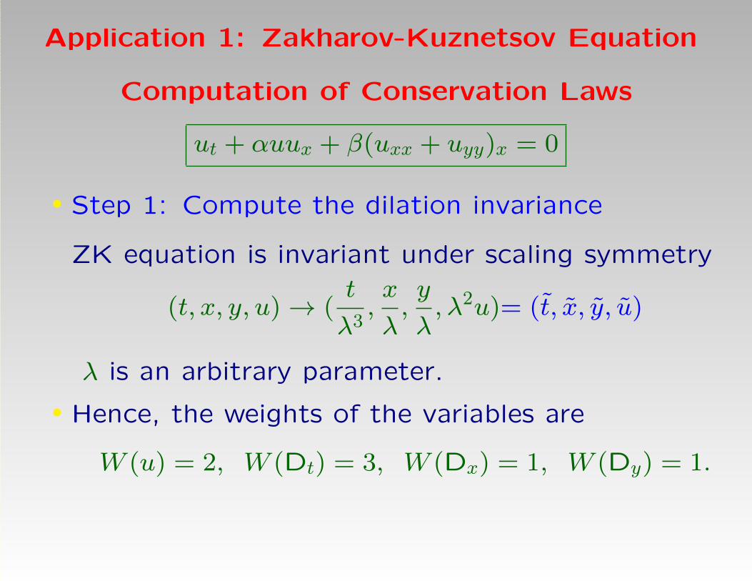
Application 1: Zakharov-Kuznetsov Equation

Computation of Conservation Laws

ut + αuux + β(uxx + uyy)x = 0

• Step 1: Compute the dilation invariance

ZK equation is invariant under scaling symmetry

(t, x, y, u)→ (t

λ3,x

λ,y

λ, λ2u)= (t, x, y, u)

λ is an arbitrary parameter.

• Hence, the weights of the variables are

W (u) = 2, W (Dt) = 3, W (Dx) = 1, W (Dy) = 1.

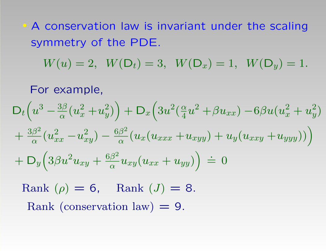
• A conservation law is invariant under the scaling

symmetry of the PDE.

W (u) = 2, W (Dt) = 3, W (Dx) = 1, W (Dy) = 1.

For example,

Dt

(u3 − 3β

α(u2

x +u2y))

+ Dx

(3u2(α

4u2 +βuxx)−6βu(u2

x + u2y)

+ 3β2

α(u2

xx −u2xy)−

6β2

α(ux(uxxx +uxyy) + uy(uxxy +uyyy))

)+ Dy

(3βu2uxy + 6β2

αuxy(uxx + uyy)

)= 0

Rank (ρ) = 6, Rank (J) = 8.

Rank (conservation law) = 9.

Compute the density of selected rank, say, 6.

• Step 2: Construct the candidate density

For example, construct a density of rank 6.

Make a list of all terms with rank 6:

u3, u2x, uuxx, u

2y, uuyy, uxuy, uuxy, u4x, u3xy, u2x2y, ux3y, u4y

Remove divergences and divergence-equivalentterms.

Candidate density of rank 6:

ρ = c1u3 + c2u

2x + c3u

2y + c4uxuy

• Step 3: Compute the undetermined coefficients

Compute

Dtρ=∂ρ

∂t+ ρ′(u)[ut]

=∂ρ

∂t+

Mx∑k=0

My∑`=0

∂ρ

∂ukx `yDkx D`

y ut

=(

3c1u2I + 2c2uxDx + 2c3uyDy + c4(uyDx + uxDy)

)ut

Substitute ut = −(αuux + β(uxx + uyy)x

).

E = −Dtρ = 3c1u2(αuux + β(uxx + uxy)x)

+ 2c2ux(αuux + β(uxx + uyy)x)x + 2c3uy(αuux

+ β(uxx + uyy)x)y + c4(uy(αuux + β(uxx + uyy)x)x

+ ux(αuux + β(uxx + uyy)x)y)

Apply the Euler operator (variational derivative)

Lu(x,y)E =

Mx∑k=0

My∑`=0

(−Dx)k(−Dy)

` ∂E

∂ukx `y

=−2(

(3c1β + c3α)uxuyy + 2(3c1β + c3α)uyuxy

+2c4αuxuxy +c4αuyuxx +3(3c1β +c2α)uxuxx)

≡ 0

Solve a parameterized linear system for the ci:

3c1β + c3α = 0, c4α = 0, 3c1β + c2α = 0

Solution:

c1 = 1, c2 = −3βα, c3 = −3β

α, c4 = 0

Substitute the solution into the candidate density

ρ = c1u3 + c2u

2x + c3u

2y + c4uxuy

Final density of rank 6:

ρ = u3 −3β

α(u2

x + u2y)

• Step 4: Compute the flux

Use the homotopy operator to invert Div:

J=Div−1E=(H(x)u(x,y)E, H

(y)u(x,y)E

)where

H(x)u(x,y)E =

∫ 1

0(I(x)u E)[λu]

dλ

λ

with

I(x)u E =

Mx∑k=1

My∑`=0

( k−1∑i=0

∑j=0

uix jy

(i+ji

)(k+`−i−j−1k−i−1

)(k+`k

)(−Dx)

k−i−1 (−Dy

)`−j ) ∂E

∂ukx `y

Similar formulas for H(y)u(x,y)E and I(y)

u E.

Let A = αuux + β(uxxx + uxyy) so that

E = 3u2A− 6βαuxAx − 6β

αuyAy

Then,

J =(H(x)u(x,y)E, H

(y)u(x,y)E

)=(

3α4u4 + βu2(3uxx + 2uyy)− 2βu(3u2

x + u2y)

+ 3β2

4αu(u2x2y + u4y)− β2

αux(

72uxyy + 6uxxx)

− β2

αuy(4uxxy + 3

2uyyy) + β2

α(3u2

xx + 52u2xy + 3

4u2yy)

+ 5β2

4αuxxuyy, βu2uxy − 4βuuxuy

− 3β2

4αu(ux3y + u3xy)− β2

4αux(13uxxy + 3uyyy)

− 5β2

4αuy(uxxx + 3uxyy) + 9β2

4αuxy(uxx + uyy)

)

Application 2: Shallow Water Wave Equations

Computation of Conservation Laws

Quick Recapitulation

• Conservation law in (2+1) dimensions

Dtρ+∇·J = Dtρ+ DxJ1 + DyJ2 = 0

conserved density ρ and flux J = (J1, J2)

• Example: Shallow water wave (SWW) equations

ut + uux + vuy − 2 Ωv + 12hθx + θhx = 0

vt + uvx + vvy + 2 Ωu+ 12hθy + θhy = 0

θt + uθx + vθy = 0

ht + hux + uhx + hvy + vhy = 0

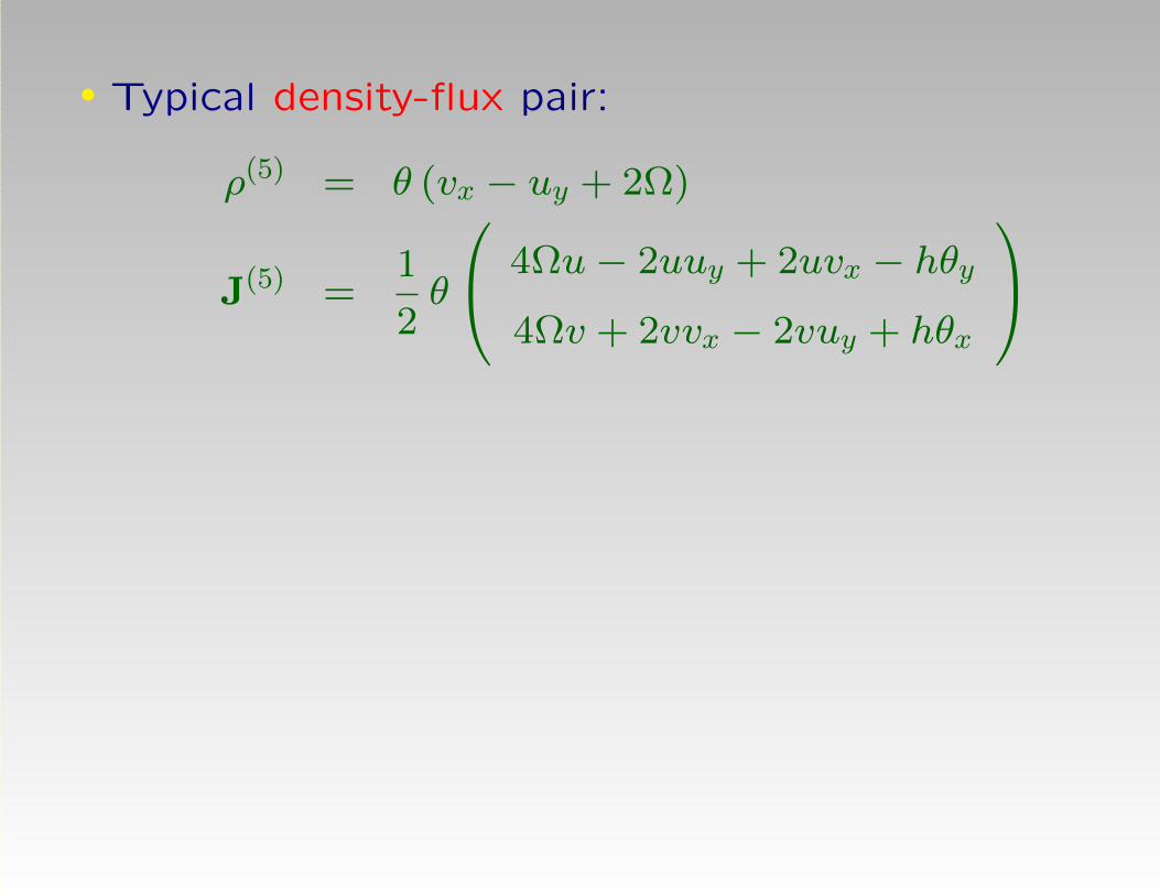
• Typical density-flux pair:

ρ(5) = θ (vx − uy + 2Ω)

J(5) =1

2θ

4Ωu− 2uuy + 2uvx − hθy4Ωv + 2vvx − 2vuy + hθx

• Step 1: Construct the form of the density

The SWW equations are invariant under the

scaling symmetries

(x, y, t, u, v, θ, h,Ω)→ (λ−1x, λ−1y, λ−2t, λu, λv, λθ, λh, λ2Ω)

and

(x, y, t, u, v, θ, h,Ω)→(λ−1x, λ−1y, λ−2t, λu, λv, λ2θ, λ0h, λ2Ω)

Construct a candidate density, for example,

ρ = c1Ωθ + c2uyθ + c3vyθ + c4uxθ + c5vxθ

which is scaling invariant under both symmetries.

• Step 2: Determine the constants ci

Compute E = −Dtρ and remove time derivatives

E = −(∂ρ

∂uxutx +

∂ρ

∂uyuty +

∂ρ

∂vxvtx +

∂ρ

∂vyvty +

∂ρ

∂θθt)

= c4θ(uux + vuy − 2Ωv + 12hθx + θhx)x

+ c2θ(uux + vuy − 2Ωv + 12hθx + θhx)y

+ c5θ(uvx + vvy + 2Ωu+ 12hθy + θhy)x

+ c3θ(uvx + vvy + 2Ωu+ 12hθy + θhy)y

+ (c1Ω + c2uy + c3vy + c4ux + c5vx)(uθx + vθy)

Require that

Lu(x,y)E = Lv(x,y)E = Lθ(x,y)E = Lh(x,y)E ≡ 0.

• Solution: c1 = 2, c2 = −1, c3 = c4 = 0, c5 = 1 gives

ρ = ρ(5) = θ (2Ω− uy + vx)

• Step 3: Compute the flux J

E = θ(uxvx + uvxx + vxvy + vvxy + 2Ωux

+12θxhy − uxuy − uuxy − uyvy − uyyv

+2Ωvy − 12θyhx) + 2Ωuθx + 2Ωvθy

−uuyθx − uyvθy + uvxθx + vvxθy

Apply the 2D homotopy operator:

J = (J1, J2) = Div−1E = (H(x)u(x,y)E,H

(y)u(x,y)E)

Compute

I(x)u E = u

∂E

∂ux+(

12uyI− 1

2uDy

) ∂E

∂uxy

= uvxθ + 2Ωuθ + 12u2θy − uuyθ

Similarly, compute

I(x)v E = vvyθ + 1

2v2θy + uvxθ

I(x)θ E = 1

2θ2hy + 2Ωuθ − uuyθ + uvxθ

I(x)h E = −1

2θθyh

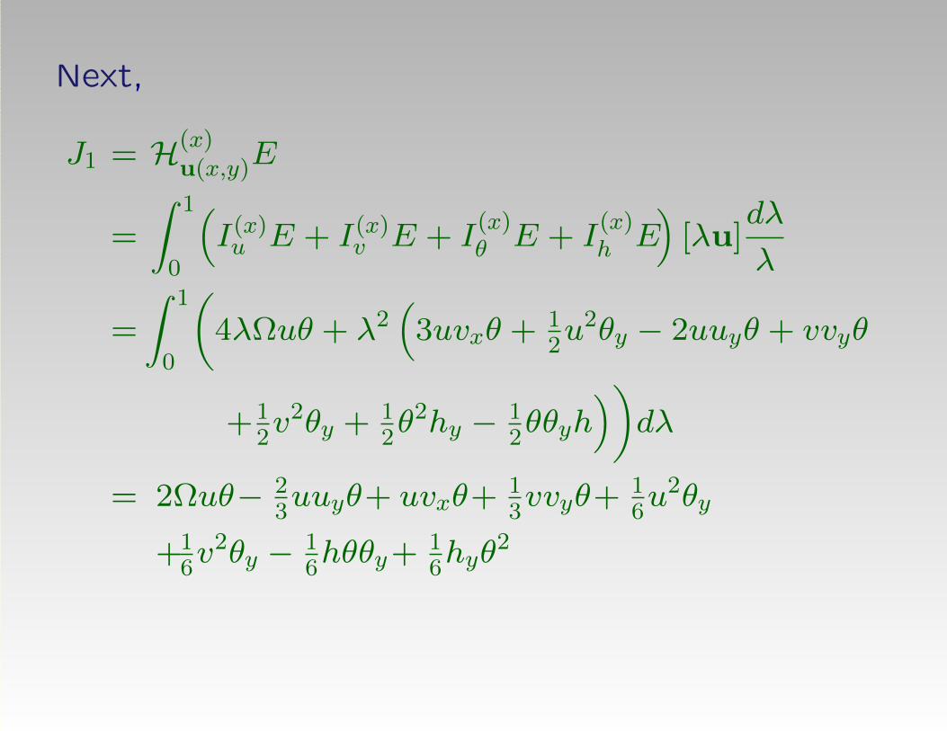
Next,

J1 = H(x)u(x,y)E

=

∫ 1

0

(I(x)u E + I(x)

v E + I(x)θ E + I

(x)h E

)[λu]

dλ

λ

=

∫ 1

0

(4λΩuθ + λ2

(3uvxθ + 1

2u2θy − 2uuyθ + vvyθ

+12v2θy + 1

2θ2hy − 1

2θθyh

))dλ

= 2Ωuθ− 23uuyθ+ uvxθ+ 1

3vvyθ+ 1

6u2θy

+16v2θy − 1

6hθθy+ 1

6hyθ

2

Analogously,

J2 = H(y)u(x,y)E

= 2Ωvθ + 23vvxθ − vuyθ − 1

3uuxθ − 1

6u2θx − 1

6v2θx

+16hθθx − 1

6hxθ

2

Hence,

J = J(5) =

1

6

12Ωuθ−4uuyθ+6uvxθ+2vvyθ+(u2+v2)θy−hθθy+hyθ2

12Ωvθ+4vvxθ−6vuyθ−2uuxθ−(u2+v2)θx+hθθx−hxθ2

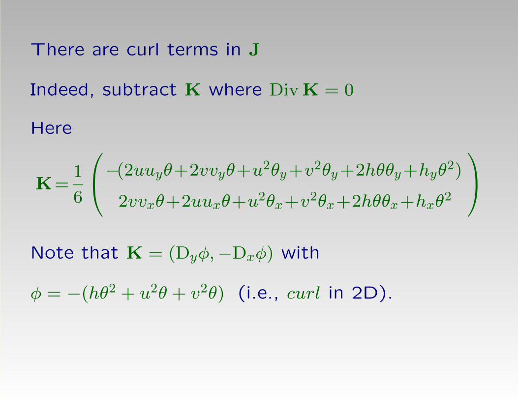
There are curl terms in J

Indeed, subtract K where Div K = 0

Here

K=1

6

−(2uuyθ+2vvyθ+u2θy+v2θy+2hθθy+hyθ2)

2vvxθ+2uuxθ+u2θx+v2θx+2hθθx+hxθ2

Note that K = (Dyφ,−Dxφ) with

φ = −(hθ2 + u2θ + v2θ) (i.e., curl in 2D).

After removing the curl term K,

J = J(5) =1

2θ

4Ωu− 2uuy + 2uvx − hθy4Ωv + 2vvx − 2vuy + hθx

PART II: DISCRETE CASE

Problem Statement

Discrete case in 1D:

Example:

fn=−unun+1vn−v2n+un+1un+2vn+1+v2

n+1+un+3vn+2−un+1vn

Question: Can the expression be summed by parts?

If yes, find Fn = ∆−1fn (so, fn = ∆Fn = Fn+1 − Fn)

Result (by hand):

Fn=v2n + unun+1vn + un+1vn + un+2vn+1

How can this be done algorithmically?

Can this be done as in the continuous case?

Tools from the Discrete Calculus of Variations

• Definitions:

D is the up-shift (forward or right-shift) operator

DFn = Fn+1 = Fn|n→n+1

D−1 the down-shift (backward or left-shift) operator

D−1Fn = Fn−1 = Fn|n→n−1

∆ = D− I is the forward difference operator

∆Fn = (D− I)Fn = Fn+1 − Fn

• Problem to be solved: Given fn.

Find Fn = ∆−1fn (so fn = ∆Fn = Fn+1 − Fn)

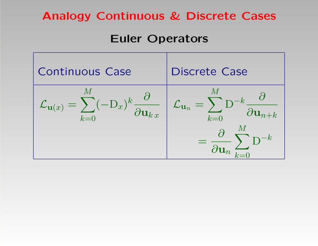
Analogy Continuous & Discrete Cases

Euler Operators

Continuous Case Discrete Case

Lu(x) =M∑k=0

(−Dx)k ∂

∂uk xLun =

M∑k=0

D−k∂

∂un+k

=∂

∂un

M∑k=0

D−k

Analogy Continuous & Discrete Cases

Homotopy Operators & Integrands

Continuous Case Discrete Case

Hu(x)f=

∫ 1

0

N∑j=1

(Iu(j)f)[λu]dλ

λHunfn=

∫ 1

0

N∑j=1

(Iu(j)nfn)[λun]

dλ

λ

Iu(j)f =

M(j)∑k=1

Iu(j)nfn =

M(j)∑k=1k−1∑

i=0

u(j)ix (−Dx)k−(i+1)

∂f

∂u(j)kx

k∑i=1

D−iu(j)

n+k

∂fn

∂u(j)n+k

Euler Operators Side by Side

Continuous Case (for component u)

Lu=∂

∂u−Dx

∂

∂ux+ D2

x

∂

∂u2x−D3

x

∂

∂u3x+ · · ·

Discrete Case (for component un)

Lun =∂

∂un+ D−1 ∂

∂un+1+ D−2 ∂

∂un+2+ D−3 ∂

∂un+3+ · · ·

=∂

∂un(I + D−1 + D−2 + D−3 + · · · )

Homotopy Operators Side by Side

Continuous Case (for components u and v)

Hu(x)f =

∫ 1

0(Iu f + Iv f) [λu]

dλ

λ

with

Iu f =M(1)∑k=1

k−1∑i=0

uix (−Dx)k−(i+1)

∂f

∂ukx

and

Iv f =M(2)∑k=1

k−1∑i=0

vix (−Dx)k−(i+1)

∂f

∂vkx

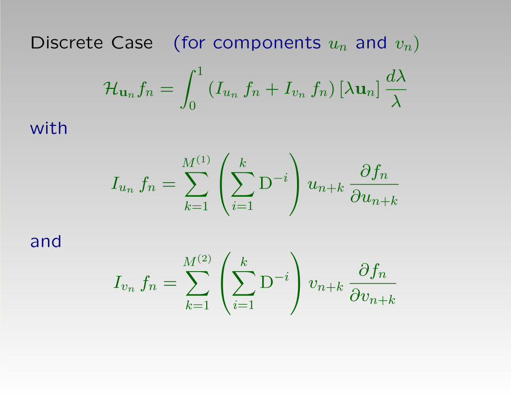
Discrete Case (for components un and vn)

Hunfn =

∫ 1

0(Iun fn + Ivn fn) [λun]

dλ

λ

with

Iun fn =M(1)∑k=1

k∑i=1

D−i

un+k∂fn

∂un+k

and

Ivn fn =M(2)∑k=1

k∑i=1

D−i

vn+k∂fn

∂vn+k

Analogy of Definitions & Theorems

Continuous Case (PDE) Semi-discrete Case (DDE)

ut=F(u,ux,u2x, · · · ) un=F(· · · ,un−1,un,un+1, · · · )

Dtρ+ DxJ = 0 Dtρn + ∆ Jn = 0

• Definition: fn is exact iff fn = ∆Fn = Fn+1 − Fn• Theorem (exactness test): fn = ∆Fn iff Lun fn ≡ 0

• Theorem (summation with homotopy operator):

If fn is exact then Fn = ∆−1fn = Hun(fn)

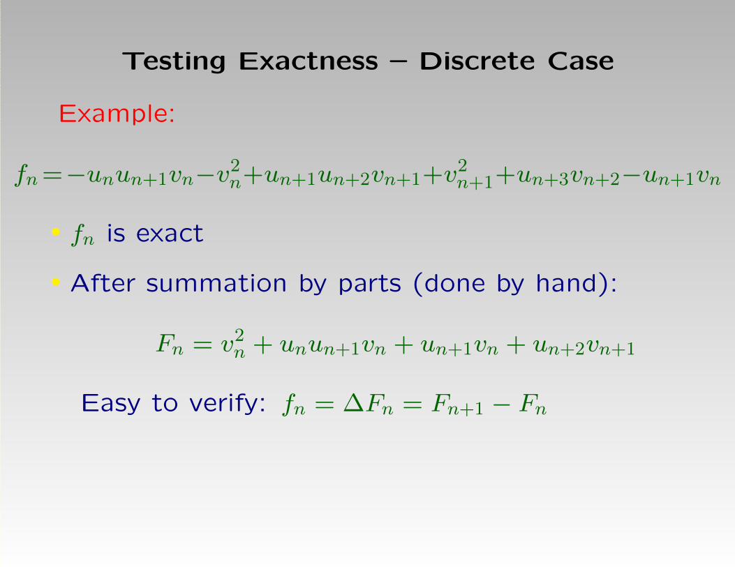
Testing Exactness – Discrete Case

Example:

fn=−unun+1vn−v2n+un+1un+2vn+1+v2

n+1+un+3vn+2−un+1vn

• fn is exact

• After summation by parts (done by hand):

Fn = v2n + unun+1vn + un+1vn + un+2vn+1

Easy to verify: fn = ∆Fn = Fn+1 − Fn

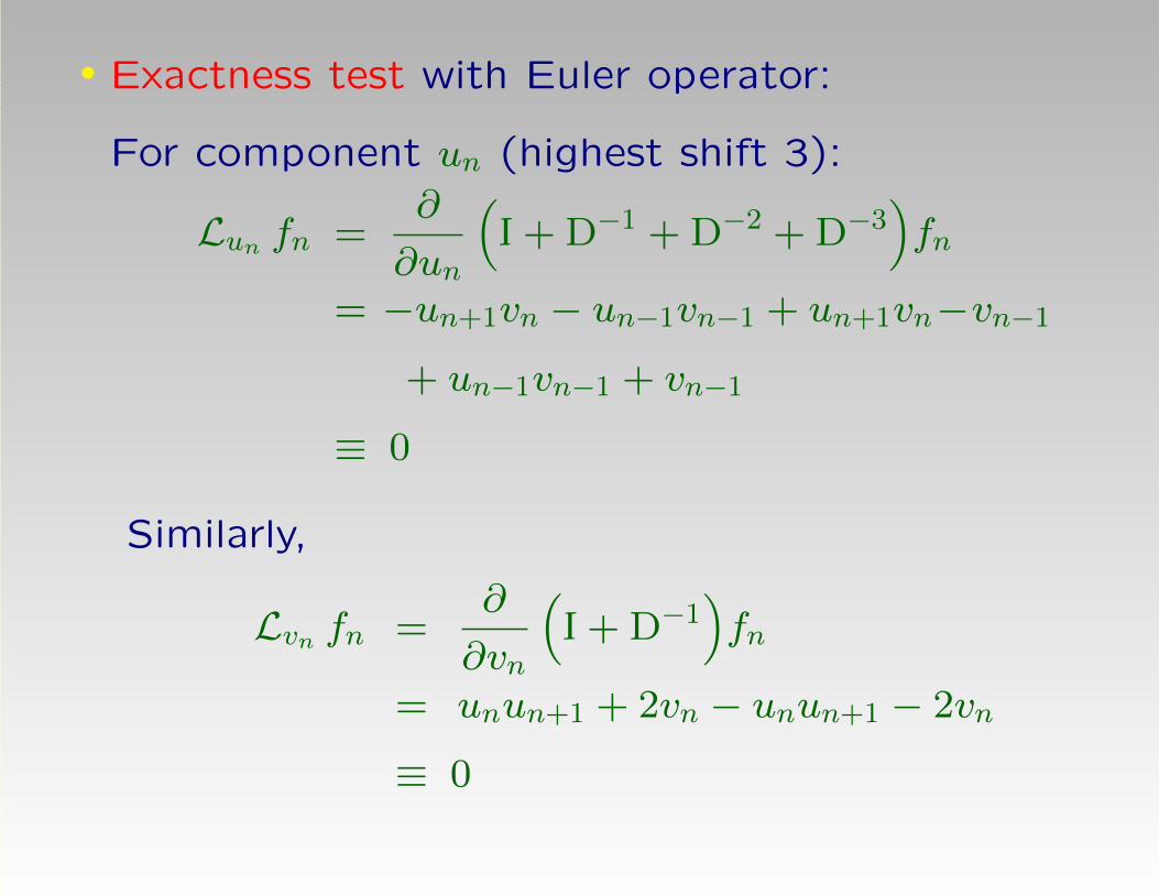
• Exactness test with Euler operator:

For component un (highest shift 3):

Lun fn =∂

∂un

(I + D−1 + D−2 + D−3

)fn

= −un+1vn − un−1vn−1 + un+1vn−vn−1

+ un−1vn−1 + vn−1

≡ 0

Similarly,

Lvn fn =∂

∂vn

(I + D−1

)fn

= unun+1 + 2vn − unun+1 − 2vn

≡ 0

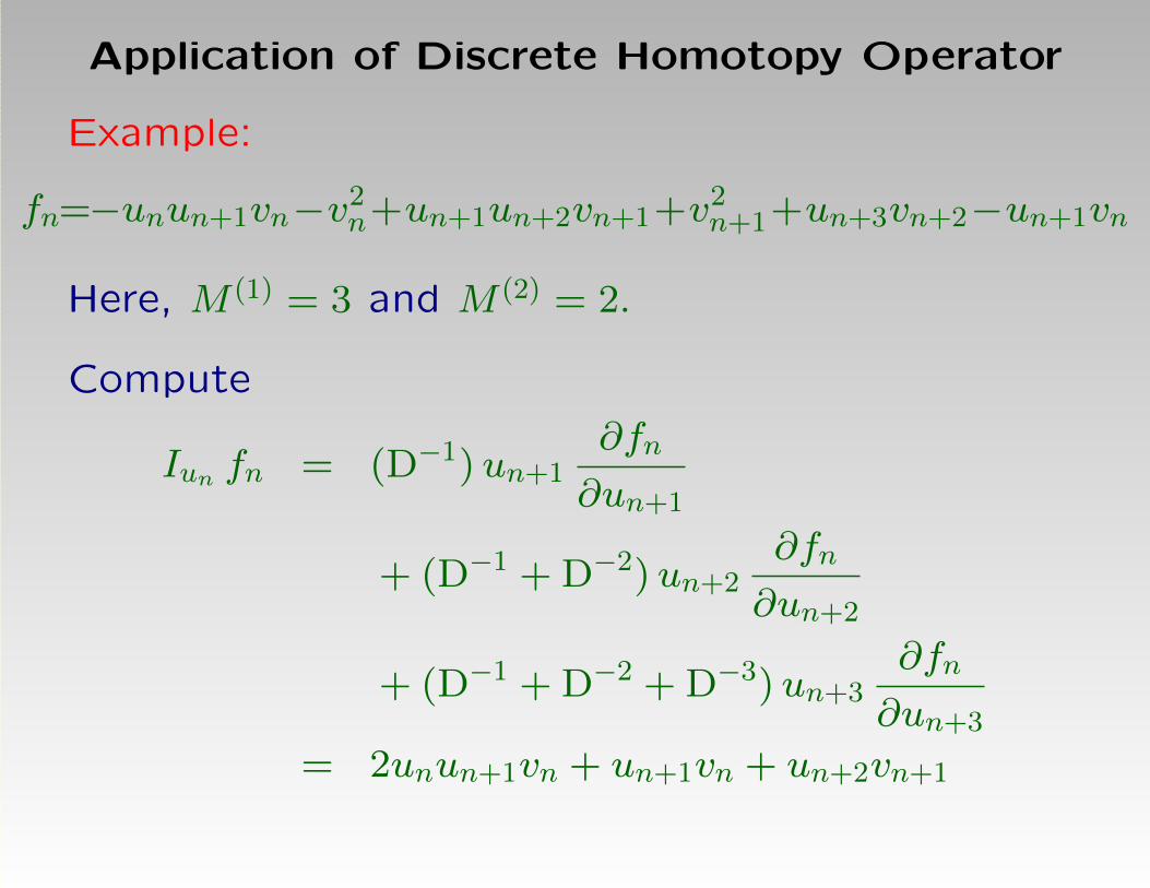
Application of Discrete Homotopy Operator

Example:

fn=−unun+1vn−v2n+un+1un+2vn+1+v2

n+1+un+3vn+2−un+1vn

Here, M (1) = 3 and M (2) = 2.

Compute

Iun fn = (D−1)un+1∂fn

∂un+1

+ (D−1 + D−2)un+2∂fn

∂un+2

+ (D−1 + D−2 + D−3)un+3∂fn

∂un+3

= 2unun+1vn + un+1vn + un+2vn+1

Ivn fn = (D−1) vn+1∂fn

∂vn+1

+ (D−1 + D−2) vn+2∂fn

∂vn+2

= unun+1vn + 2v2n + un+1vn + un+2vn+1

Finally,

Fn =

∫ 1

0(Iun fn + Ivn fn) [λun]

dλ

λ

=

∫ 1

0

(2λv2

n + 3λ2unun+1vn + 2λun+1vn + 2λun+2vn+1

)dλ

= v2n + unun+1vn + un+1vn + un+2vn+1

Application: Computation of Conservation Laws

• System of DDEs

un=F(· · · ,un−1,un,un+1, · · · )

• Conservation law

Dtρn + ∆Jn = 0

conserved density ρn and flux Jn

• Example: Toda lattice

un = vn−1 − vnvn = vn(un − un+1)

• Typical density-flux pair:

ρ(3)n = 1

3u3n + un(vn−1 + vn)

J (3)n = un−1unvn−1 + v2

n−1

Computation Conservation Laws for Toda Lattice

Step 1: Construct the form of the density

The Toda lattice is invariant under scaling symmetry

(t, un, vn)→ (λ−1t, λun, λ2vn)

Construct a candidate density, for example,

ρn = c1 u3n + c2 unvn−1 + c3 unvn

which is scaling invariant under the symmetry

Step 2: Determine the constants ci

Compute En = Dtρn and remove time derivatives

En = (3c1 − c2)u2nvn−1 + (c3 − 3c1)u2

nvn + (c3 − c2)vn−1vn

+c2un−1unvn−1 + c2v2n−1 − c3unun+1vn − c3v

2n

Compute En = DEn to remove negative shift n− 1

Require that Lun En = Lvn En ≡ 0

Solution: c1 = 13, c2 = c3 = 1 gives

ρn = ρ(3)n = 1

3u3n + un(vn−1 + vn)

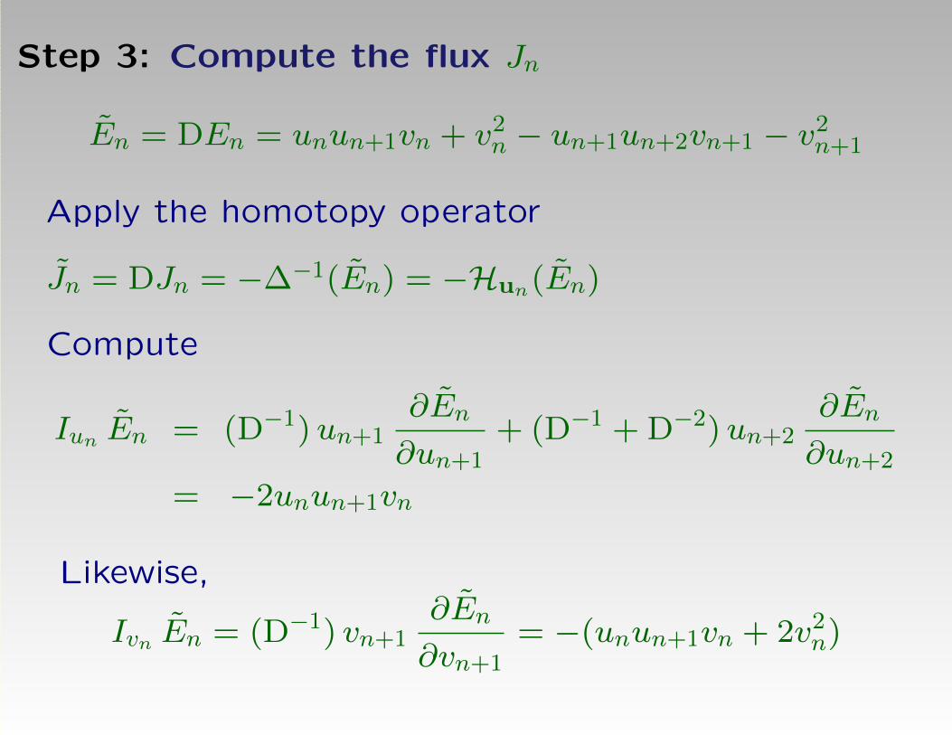
Step 3: Compute the flux Jn

En = DEn = unun+1vn + v2n − un+1un+2vn+1 − v2

n+1

Apply the homotopy operator

Jn = DJn = −∆−1(En) = −Hun(En)

Compute

Iun En = (D−1)un+1∂En

∂un+1+ (D−1 + D−2)un+2

∂En

∂un+2

= −2unun+1vn

Likewise,

Ivn En = (D−1) vn+1∂En

∂vn+1= −(unun+1vn + 2v2

n)

Next, compute

Jn = −∫ 1

0

(Iun En + Ivn En

)[λun]

dλ

λ

=

∫ 1

0(3λ2unun+1vn + 2λv2

n) dλ

= unun+1vn + v2n

Finally, backward shift Jn = D−1(Jn) given

Jn = J (3)n = un−1unvn−1 + v2

n−1

Conclusions and Future Work

• The power of Euler and homotopy operators:

I Testing exactness

I Integration by parts: D−1x and Div−1

• Integration of non-exact expressions

Example: f = uxv + uvx + u2uxx∫fdx = uv +

∫u2uxx dx

• Use other homotopy formulas (moving terms

amongst the components of the flux; prevent curl

terms)

• Homotopy operator approach pays off for

computing irrational fluxes

Example: short pulse equation (nonlinear optics)

uxt = u+ (u3)xx = u+ 6uu2x + 3u2uxx

with non-polynomial conservation law

Dt

(√1 + 6u2

x

)−Dx

(3u2√

1 + 6u2x

)= 0

• Continue the implementation in Mathematica

• Software: http://inside.mines.edu/∼whereman

Thank You

Publications

1. D. Poole and W. Hereman, Symbolic computation

of conservation laws for nonlinear partial

differential equations in multiple space dimensions,

J. Symb. Comp. 46(12), 1355-1377 (2011).

2. W. Hereman, P. J. Adams, H. L. Eklund, M. S.

Hickman, and B. M. Herbst, Direct Methods and

Symbolic Software for Conservation Laws of

Nonlinear Equations, In: Advances of Nonlinear

Waves and Symbolic Computation, Ed.: Z. Yan,

Nova Science Publishers, New York (2009),

Chapter 2, pp. 19-79.

3. W. Hereman, M. Colagrosso, R. Sayers, A.

Ringler, B. Deconinck, M. Nivala, and M. S.

Hickman, Continuous and Discrete Homotopy

Operators and the Computation of Conservation

Laws. In: Differential Equations with Symbolic

Computation, Eds.: D. Wang and Z. Zheng,

Birkhauser Verlag, Basel (2005), Chapter 15, pp.

249-285.

4. W. Hereman, B. Deconinck, and L. D. Poole,

Continuous and discrete homotopy operators:

A theoretical approach made concrete, Math.

Comput. Simul. 74(4-5), 352-360 (2007).

5. W. Hereman, Symbolic computation of

conservation laws of nonlinear partial differential

equations in multi-dimensions, Int. J. Quan.

Chem. 106(1), 278-299 (2006).