Application of Electrical and Radioactive Well Logging to ... · PDF fileApplication of...
66
Application of Electrical and Radioactive Well Logging to Ground-Water Hydrology GEOLOGICAL SURVEY WATER-SUPPLY PAPER 1544-D Prepared in cooperation with the Pennsylvania Geological Survey Department of Internal Affairs Commonwealth of Pennsylvania
Transcript of Application of Electrical and Radioactive Well Logging to ... · PDF fileApplication of...
Application of Electrical and Radioactive Well Logging to Ground-Water Hydrology
GEOLOGICAL SURVEY WATER-SUPPLY PAPER 1544-D
Prepared in cooperation with the Pennsylvania Geological Survey Department of Internal Affairs Commonwealth of Pennsylvania

Application of Electrical and Radioactive Well Logging to Ground-Water HydrologyBy EUGENE P. PATTEN, JR., and GORDON D. BENNETT
GENERAL GROUND-WATER TECHNIQUES
GEOLOGICAL SURVEY WATER-SUPPLY PAPER 1544-D
Prepared in cooperation with the Pennsylvania Geological Survey Department of Internal Affairs Commonwealth of Pennsylvania
UNITED STATES GOVERNMENT PRINTING OFFICE, WASHINGTON : 1963
UNITED STATES DEPARTMENT OF THE INTERIOR
STEWART L. UDALL, Secretary
GEOLOGICAL SURVEY
William T. Pecora, Director
First printing 1963 Second printing 1967
For sale by the Superintendent of Documents, U.S. Government Printing Office Washington, D.C. 20402 - Price 25 cents (paper cover)

CONTENTS
Page Abstract___ __________-____-______-..--__-_-_-________--_____,___ D-1Introduction..,.________ ___-___-_-_--_----___-_-___-_______-___ 1Resistivity logging________ -__----_____---__-____--__-_--_-_ 2
Instrumentation and theory__________________________________ 2Calibration and zones of investigation______________________ 6Borehole effect__________________________________________._ 7
Mechanism of electrical conduction in earth materials._____________ 9General lithologic interpretation...........______________________ 10Interpretation based upon the relative magnitudes of the normal
curves.. _ _______________________________________ 11Interpretative practices in the oil industry.___________________ 11Conditions in a mud-filled borehole...-...-----..--.-------.. 13Conditions in a water-filled borehole......-..---------------- 14Summary of interpretation of the relative magnitude of normal
curves______________.___-_____-___.____-_____-_-_--_ 18Relation of porosity to formation factor_______-_______-._ __.. 18Recognition of secondary porosity in limestone and crystalline rocks. _ 20Secondary porosity in sandstone-shale sections-________--____-__-- 24
Spontaneous-potential logging.______________________________________ 26Instrumentation ___ _________________-_-___---_-_-_--__---_-. 26History...__________________________________________ 27Analysis of quantitative interpretation______._________--___--_-__ 27
The general liquid-junction equation-__-____--___-_-_-_--_--- 29Equation for direct junction between two sodium chloride
solutions._____._.________-_-_____-_____-__------------_ 30Junction of sodium chloride solutions through an ion-selective
membrane....______._________--_-___-___---_-____-__ 30Role of shale as an ion-selective membrane ___________________ 31Liquid-junction potentials in an oil well______________________ 32Relation of the spontaneous-potential measurement to the theo
retical electromotive force_-__-__-------_--------_-------- 34Objections to quantitative interpretation for water wells__________ 36Interaquifer flow_______._______________-______-_----_------_-_ 37Streaming potentials..________._______-_____-__---___-.-_-.- 38Zones containing highly mineralized water.______--___--_-_-_---__ 38Artificially induced spontaneous-potential deflections-__----_-_----_ 39Abnormal spontaneous-potential deflections.______________________ 39Summary of spontaneous-potential logging______________________ 39
Fluid-conductivity logging______________-_________-___----_.-_ 40Factors controlling conductivity......_________________________ 40Interpretation of fluid-conductivity logging in a single-aquifer well 40Interpretation of fluid-conductivity logging in a multiaquifer well... 41
in
IV CONTENTS
Page Gamma-ray logging,_______________________________________________ D-15
General discussion of radiation and gamma-ray-logging instrumenta tion_____________________________________________________ 45
Sources of radiation in common sediments________________________ 47Shale and clay____________-___-__..___-__-__--_____________ 47Sandstone.________-_______--___---_______--___________.__ 49Carbonate rocks____._____--___-_--_--_-_---__-_.__-_____ 50Evaporite rocks and coal_____-_-_----_----_-------_----____ 50
General lithologicinterpretation_____________-____---_--___-_____ 51Gamma-ray interpretation as a supplement to resistivity data.______ 51
Assumptions underlying the method-________________________ 52Interrelation of gamma radiation, formation factor and porosity
under the assumed conditions________--__--____---__-_____ 53Graphical method of interpretation__-_--___---___-__________ 54
Conclusion_____________________________________________________ 57References__----___--__-____-____--___--___-____-_______________ 57Index__________________________________________________________ 58
ILLUSTKATIONS
PageFIGURE 1. Equipment and current patterns, logging in a homogeneous
medium. ____________________________ ____ ______ D-32. Diagram showing division of medium into spherical shells
which act as resistances in series__---_-_----_--_-_--____ 43. Zones of investigation of the resistivity devices in a homo
geneous medium__________ ___. 84. Internal flow in a multiaquifer well___ __ 155. Resistivity curves opposite a zone of thin alternating beds of
sand and shale_________ 176. Current pattern, logging in a limestone or crystalline section.. 227. Resistivity curves for a water well in limestone____ ____ 258. Resistivity curves for a water well in crystalline rocks___-_-_ 269. Spontaneous-potential current and electromotive-force pat
tern at a sand-shale contact -- ________ 3310. Fluid-conductivity log in a multiaquifer well in which ionic
diffusion is negligible--..--.------------------- -- - 4211. Graph showing interrelation of radiation, formation factor,
and porosity in an ideal sedimentary section ______ _ 54
GENERAL GROUND-WATER TECHNIQUES
APPLICATION OF ELECTRICAL AND RADIOACTIVE WELL LOGGING TO GROUND-WATER HYDROLOGY
By EUGENE P. PATTEN, JR., and GORDON D. BENNETT
ABSTRACT
This report discusses in detail several problems pertaining to the interpreta tion of electrical and radioactive well logs in ground-water hydrology. Emphasis has been placed upon situations in which interpretation departs from the practices common in petroleum engineering. Certain interpretive methods of the oil industry are demonstrated to be unsatisfactory for hydrologic pur poses, and certain other methods which have not been significant in the oil industry are recommended for use in ground-water hydrology. For all methods, an effort has been made to analyze the interpretive methods in terms of under lying theory, as an understanding of theory is superior to any memorized set of rules or principles in analyzing the data of well logging.
INTRODUCTION
Electrical and radioactive well logging has come into widespread use in ground-water hydrology during recent years, and many articles have been published dealing with its application in this field. Most of these articles are general and do not treat particular interpretive probems in detail.
This report is one of several resulting from an investigation of subsurface geophysical methods made by the U.S. Geological Sur vey in cooperation with the Pennsylvania Geological Survey.
The report is not intended as a comprehensive manual of log inter pretation but, rather, as a discussion of selected problems of interest to the ground-water hydrologist. Special attention has been given to differences in interpretative practice between oil-reservoir and ground-water investigations. Such differences may arise when the assumptions underlying the interpretive techniques of the oil in dustry cannot be extended to hydrologic work, or when the objectives of interpretation differ between the two situations.
D-l
D-2 GENERAL GROUND-WATER TECHNIQUES
Many aspects of lithologic interpretation are basically the same in ground-water and oil-reservoir studies; most of these are not treated in detail in this report, as they are described adequately in the litera ture of the oil industry and are well known to ground-water hydrologists.
RESISTIVITY LOGGING
The following discussion of resistivity logging is confined to the single-point resistance and normal arrangement, multiple-electrode resistivity methods. Although these have been supplemented by ad vanced electric-logging techniques in the oil industry, they remain the most popular methods of logging in hydrologic work. It is doubtful that the application of advanced electric-logging techniques to ground-water problems would yield information of equivalent or greater value, at the present time. Most of the new techniques were developed to deal with reservoir or borehole conditions that are not common in ground-water studies. It seems preferable that advances in instrumentation in the ground-water field follow a somewhat different line, according to the specialized problems of the field.
Although this report is not comprehensive, it includes a section on the general theory of resistivity logging to prepare the reader for the discussion of interpretive problems. An understanding of inter pretive methods in logging is impossible without a general knowledge of the underlying electrical theory. The theory presented here follows that given by Guyod (1952) for single-point and normal- resistivity devices.
INSTRUMENTATION AND THEORY
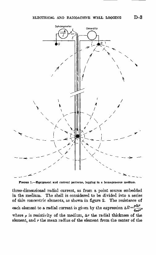
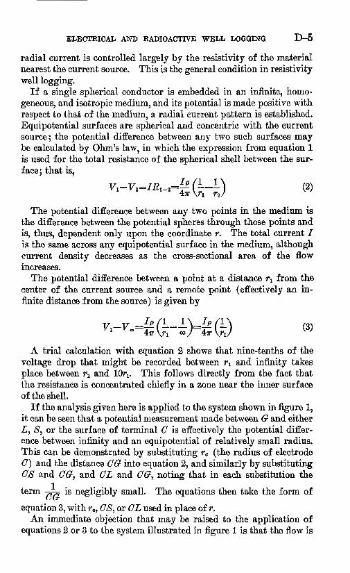
A typical logging apparatus might be arranged according to the diagram of figure 1. A constant current is maintained between the two spherical terminals G and Z>, and a recording galvanometer may be set to read the voltage between G and either <7, $, or L. The dis tance OS is approximately 16 inches, and OL is approximately 64 inches. The distances CD and CG are large relative to OS and OL. If the galvanometer is set to read the potential difference between 0 and £r, the apparatus is termed a single-point device; if it is set to read the potential between S and G, the apparatus is called a short- normal device; and if it is set between L and 6f, the apparatus is a long-normal device.
If the earth and well bore are considered to be an infinite, homo geneous, and isotropic electrical medium, a simplified mathematical treatment is possible. To begin this treatment, an expression will be derived for the resistance of a spherical shell in such a medium to a
ELECTRICAL AND RADIOACTIVE WELL LOGGING D-3
GalvanometerGenerator
FIGCEH 1. Equipment and current patterns, logging In a homogeneous medium.
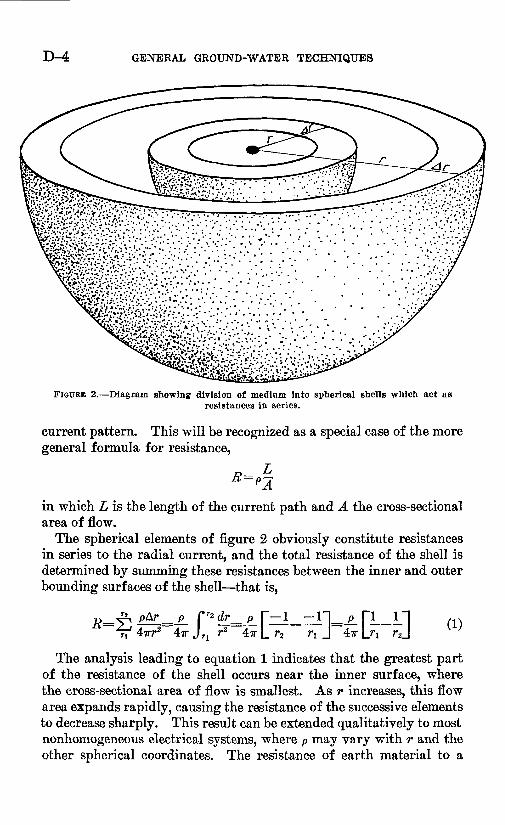
three-dimensional radial current, as from a point source embedded in the medium. The shell is considered to be divided into a series of thin concentric elements, as shown in figure 2. The resistance of
each element to a radial current is given by the expression ^R=
where p is resistivity of the medium, AT- the radial thickness of the element, and r the mean radius of the element from the center of the
D-4 GENERAL GROUND-WATER TECHNIQUES
FIGURE 2. Diagram showing division of medium into spherical shells which act asresistances in series.
current pattern. This will be recognized as a special case of the more general formula for resistance,
*->zin which L is the length of the current path and A the cross-sectional area of flow.
The spherical elements of figure 2 obviously constitute resistances in series to the radial current, and the total resistance of the shell is determined by summing these resistances between the inner and outer bounding surfaces of the shell that is,
pArr2 4
The analysis leading to equation 1 indicates that the greatest part of the resistance of the shell occurs near the inner surface, where the cross-sectional area of flow is smallest. As r increases, this flow area expands rapidly, causing the resistance of the successive elements to decrease sharply. This result can be extended qualitatively to most nonhomogeneous electrical systems, where p may vary with r and the other spherical coordinates. The resistance of earth material to a
ELECTRICAL AND RADIOACTIVE WELL LOGGING D-5
radial current is controlled largely by the resistivity of the material nearest the current source. This is the general condition in resistivity well logging.
If a single spherical conductor is embedded in an infinite, homo geneous, and isotropic medium, and its potential is made positive with respect to that of the medium, a radial current pattern is established. Equipotential surfaces are spherical and concentric with the current source; the potential difference between any two such surfaces may be calculated by Ohm's law, in which the expression from equation 1 is used for the total resistance of the spherical shell between the sur face; that is,
The potential difference between any two points in the medium is the difference between the potential spheres through those points and is, thus, dependent only upon the coordinate r. The total current / is the same across any equipotential surface in the medium, although current density decreases as the cross-sectional area of the flow increases.
The potential difference between a point at a distance TI from the center of the current source and a remote point (effectively an in finite distance from the source) is given by
A trial calculation with equation 2 shows that nine-tenths of the voltage drop that might be recorded between ^ and infinity takes place between rt and 10/v This follows directly from the fact that the resistance is concentrated chiefly in a zone near the inner surface of the shell.
If the analysis given here is applied to the system shown in figure 1, it can be seen that a potential measurement made between G and either Z, $, or the surface of terminal O is effectively the potential differ ence between infinity and an equipotential of relatively small radius. This can be demonstrated by substituting re (the radius of electrode G) and the distance CG- into equation 2, and similarly by substituting OS and CG, and GL and CG, noting that in each substitution the
term -^ is negligibly small. The equations then take the form ofOtr
equation 3, with rc, C8, or GL used in place of r.An immediate objection that may be raised to the application of
equations 2 or 3 to the system illustrated in figure 1 is that the flow is
D-6 GENERAL GROUND-WATER TECHNIQUES
between the two current terminals rather than being truly radial to an infinite distance. In order to be entirely rigorous, the effect of the current sink, or negative electrode Z>, must be considered. This can be done by deriving an expression for the potential difference between any two points because of a radial flow toward the sink, assuming it to be alone in the system. An expression of the form of equation 2 is obtained, the only difference being the use of a negative current and of distances measured from D rather than from G. The potential dif ference between any two points in the two-terminal system of figure 1 can then be calculated by scalar addition of the potential difference resulting from the operation of terminal G alone and that resulting from the operation of terminal D alone. The distances DG, LD, $Z>, and GD are all large with respect to rc, OS, and GL. Accordingly, the effect of terminal Z> on the potential difference between G and tf,
$, or Z, is negligible. Mathematically, the terms -f7f)> "OTJ» fj)» an(i
i drop out, and the equation reverts to the form of equation 3;physically, D is sufficiently remote from #, $, and L that it does not appreciably change their potential or alter the radial distribution of current in their vicinity. Thus, the analysis leading to equation 3 accurately describes the conditions in the vicinity of terminals #, $, and L of figure 1, if the earth and well bore constitute an isotropic and homogeneous electrical system. The effects of the inevitable de viations from these conditions which occur in a practical situation are discussed in later sections.
CALIBRATION AND ZONES OF INVESTIGATION
When logging is done by the single point resistance method, the galvanometer is connected between G and G. The potential measure ment made by this device, under a known current held constant by a servo-mechanism, indicates the resistance of a segment of borehole and earth extending to a radius of approximately Wrc. As has been pointed out, the potential drop beyond !Qr0 is negligible. The gal vanometer may be calibrated to read resistivity according to the formula
P =j4irrc (4)
obtained by solving the appropriate equation of the form of 3 for />. A similar analysis can be made for the short-normal arrangement,
leading to the calibration equation
ELECTRICAL AND RADIOACTIVE WELL LOGGING D-7
(5)
and for the long normal arrangement, leading to the equation
t-j**(OL) (6)
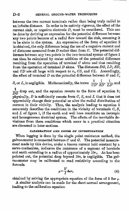
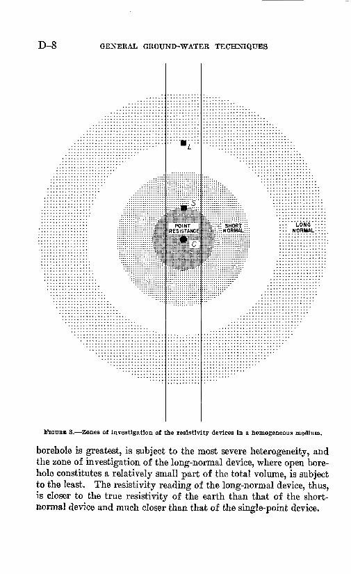
The short normal measures effectively the resistivity of a shell of borehole and earth material extending from a radius of OS to a radius approximately 1QC/S, and the long normal measures the resistivity of a shell extending from GL to 100L. Thus, each of the devices has a zone of investigation that is, a region within which a change in resistivity will produce an appreciable change in the response of the device. In practice, the zones of investigation commonly are con sidered to be even further restricted ; for example, they may be con sidered to extend from rc to 27*c, from OS to 2CS, and from GL to 2CL.
Zones of investigation of the point-resistance, short-normal, and long-normal devices are shown in figure 3, constructed assuming the borehole and earth to be a homogeneous electrical system. Figure 3 shows that much of the zone of investigation of the point- resistance device lies within the open borehole. The zone of inves tigation of the short normal includes a greater proportion of the sur rounding formation, and that of the long normal includes an even greater proportion.
Equations 4, 5, and 6 show that the logging instruments are cali brated on the assumption that the earth and borehole constitute a homogeneous medium. If this condition were met, the resistivity reading by each device obviously would be the same. If electrical heterogeneity prevails within the zone of investigation of one of the devices, the resistivity measured by that device is a composite value, its magnitude depending upon the resistivities of the component parts and the amounts and disposition of those parts within the zone of in vestigation. The zone of investigation is no longer a spherical shell, as the radial current pattern is disrupted by the electrical heteroge neity; thus the calibration equation is geometrically and physically inapplicable. Electrical heterogeneity within the zone of investi gation of one device may cause a measurable change in the response of the other devices, owing to disruption of the radial symmetry.
BOREHOLE EFFECT
In the simplest situation encountered in practice, the earth sur rounding the bore may be assumed to be perfectly homogeneous, the only heterogeneity being due to the borehole. The zone of investi gation of the point-resistance device, where the percentage of open
D-8 GENERAL GROUND-WATER TECHNIQUES
PO NT RES STANCE
"- SHORT :: : ; NORMAL!
LONG NORMAL
FIGURE 3. Zones of investigation of the resistivity devices tn a homogeneous medium.
borehole is greatest, is subject to the most severe heterogeneity, and the zone of investigation of the long-normal device, where open bore hole constitutes a relatively small part of the total volume, is subject to the least. The resistivity reading of the long-normal device, thus, is closer to the true resistivity of the earth than that of the short- normal device and much closer than that of the single-point device.
ELECTRICAL AND RADIOACTIVE WELL LOGGING D-9
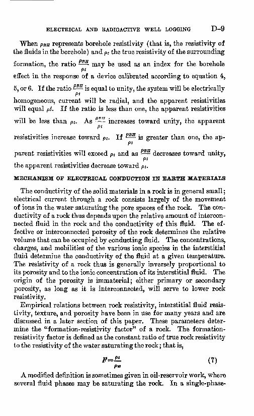
When PBH represents borehole resistivity (that is, the resistivity of the fluids in the borehole) and pt the true resistivity of the surrounding
formation, the ratio may be used as an index for the boreholept
effect in the response of a device calibrated according to equation 4,
5, or 6. If the ratio ^- is equal to unity, the system will be electrically
homogeneous, current will be radial, and the apparent resistivities will equal pt. If the ratio is less than one, the apparent resistivities
will be less than pt. As ^^ increases toward unity, the apparentpt
resistivities increase toward p t . If ^ is greater than one, the ap-pt
parent resistivities will exceed pt and as decreases toward unity,pt
the apparent resistivities decrease toward pt .
MECHANISM OP ELECTRICAL CONDUCTION IN EARTH MATERIALS
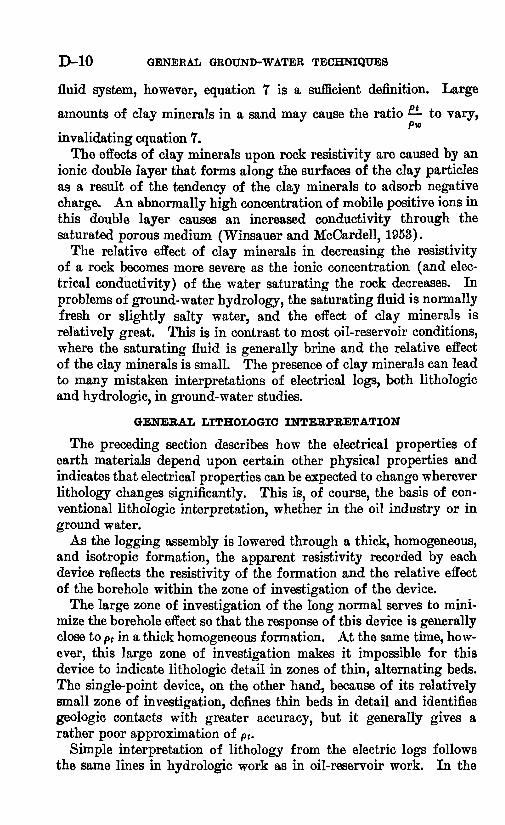
The conductivity of the solid materials in a rock is in general small; electrical current through a rock consists largely of the movement of ions in the water saturating the pore spaces of the rock. The con ductivity of a rock thus depends upon the relative amount of intercon nected fluid in the rock and the conductivity of this fluid. The ef fective or interconnected porosity of the rock determines the relative volume that can be occupied by conducting fluid. The concentrations, charges, and mobilities of the various ionic species in the interstitial fluid determine the conductivity of the fluid at a given temperature. The resistivity of a rock thus is generally inversely proportional to its porosity and to the ionic concentration of its interstitial fluid. The origin of the porosity is immaterial; either primary or secondary porosity, as long as it is interconnected, will serve to lower rock resistivity.
Empirical relations between rock resistivity, interstitial fluid resis tivity, texture, and porosity have been in use for many years and are discussed in a later section of this paper. These parameters deter mine the "formation-resistivity factor" of a rock. The formation- resistivity factor is defined as the constant ratio of true rock resistivity to the resistivity of the water saturating the rock; that is,
F-&. (7)pw
A modified definition is sometimes given in oil-reservoir work, where several fluid phases may be saturating the rock. In a single-phase-
D-10 GENERAL GROUND-WATER TECHNIQUES
fluid system, however, equation 7 is a sufficient definition. Large
amounts of clay minerals in a sand may cause the ratio to vary,PW
invalidating equation 7.The effects of clay minerals upon rock resistivity are caused by an
ionic double layer that forms along the surfaces of the clay particles as a result of the tendency of the clay minerals to adsorb negative charge. An abnormally high concentration of mobile positive ions in this double layer causes an increased conductivity through the saturated porous medium (Winsauer and McCardell, 1953).
The relative effect of clay minerals in decreasing the resistivity of a rock becomes more severe as the ionic concentration (and elec trical conductivity) of the water saturating the rock decreases. In problems of ground-water hydrology, the saturating fluid is normally fresh or slightly salty water, and the effect of clay minerals is relatively great. This is in contrast to most oil-reservoir conditions, where the saturating fluid is generally brine and the relative effect of the clay minerals is small. The presence of clay minerals can lead to many mistaken interpretations of electrical logs, both lithologic and hydrologic, in ground-water studies.
GENERAL LITHOLOGIC INTERPRETATION
The preceding section describes how the electrical properties of earth materials depend upon certain other physical properties and indicates that electrical properties can be expected to change wherever lithology changes significantly. This is, of course, the basis of con ventional lithologic interpretation, whether in the oil industry or in ground water.
As the logging assembly is lowered through a thick, homogeneous, and isotropic formation, the apparent resistivity recorded by each device reflects the resistivity of the formation and the relative effect of the borehole within the zone of investigation of the device.
The large zone of investigation of the long normal serves to mini mize the borehole effect so that the response of this device is generally close to pt in a thick homogeneous formation. At the same time, how ever, this large zone of investigation makes it impossible for this device to indicate lithologic detail in zones of thin, alternating beds. The single-point device, on the other hand, because of its relatively small zone of investigation, defines thin beds in detail and identifies geologic contacts with greater accuracy, but it generally gives a rather poor approximation of pt .
Simple interpretation of lithology from the electric logs follows the same lines in hydrologic work as in oil-reservoir work. In the
ELECTRICAL AND RADIOACTIVE WELL LOGGING D-ll
following sections special methods of interpretation that differ be tween the two fields are emphasized.
INTERPRETATION BASED UPON THE RELATIVE MAGNITUDES OF THE NORMAL CURVES
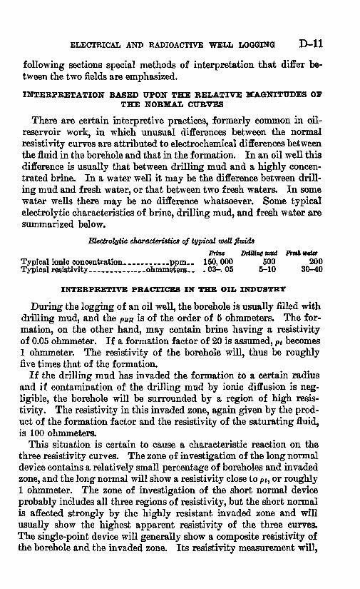
There are certain interpretive practices, formerly common in oil- reservoir work, in which unusual differences between the normal resistivity curves are attributed to electrochemical differences between the fluid in the borehole and that in the formation. In an oil well this difference is usually that between drilling mud and a highly concen trated brine. In a water well it may be the difference between drill ing mud and fresh water, or that between two fresh waters. In some water wells there may be no difference whatsoever. Some typical electrolytic characteristics of brine, drilling mud, and fresh water are summarized below.
Electrolytic characteristics of typical well fluidsPrine Drilling mvA Freth water
Typical ionic concentration_______ppm._ 150,000 500 200Typical resistivity_________ohmmeters.- . 03-. 05 5-10 30-40
INTERPRETIVE PRACTICES IN THE OIL INDUSTRY
During the logging of an oil well, the borehole is usually filled with drilling mud, and the PBH is of the order of 5 ohmmeters. The for mation, on the other hand, may contain brine having a resistivity of 0.05 ohmmeter. If a formation factor of 20 is assumed, pt becomes 1 ohmmeter. The resistivity of the borehole will, thus be roughly five times that of the formation.
If the drilling mud has invaded the formation to a certain radius and if contamination of the drilling mud by ionic diffusion is neg ligible, the borehole will be surrounded by a region of high resis tivity. The resistivity in this invaded zone, again given by the prod uct of the formation factor and the resistivity of the saturating fluid, is 100 ohmmeters.
This situation is certain to cause a characteristic reaction on the three resistivity curves. The zone of investigation of the long normal device contains a relatively small percentage of boreholes and invaded zone, and the long normal will show a resistivity close to p*, or roughly 1 ohmmeter. The zone of investigation of the short normal device probably includes all three regions of resistivity, but the short normal is affected strongly by the highly resistant invaded zone and will usually show the highest apparent resistivity of the three curves. The single-point device will generally show a composite resistivity of the borehole and the invaded zone. Its resistivity measurement will,
D-12 GENERAL GROUND-WATER TECHNIQUES
thus, be higher than the long-normal reading, but because of the strong effect of the borehole it will be less than the short-normal reading.
If the bed is not invaded by drilling fluid, the difference between the apparent resistivities shown by the long- and short-normal curves is smaller and is due only to the greater effect of the borehole in the zone of investigation of the short normal. Also, because the borehole is the more resistive of the two regions, the apparent resistiv ity of the single-point device will exceed that of the short normal.
The conditions outlined above have been used, in the oil industry, for the identification of permeable zones, on the assumption that only permeable zones will be invaded. Thus, zones for which pSN (short-normal resistivity) is observed to be much greater than pLN (long-normal resistivity) are considered to be permeable, and zones for which the two apparent resistivities are closer together, and PPR (single-point resistivity) is greater than psy, are considered to be relatively impervious.
In addition to this qualitative interpretation, the relation
PJW £m (8) PLN pw
has been used in the oil industry as a more quantitative form of inter pretation based upon the relative magnitudes of the curves. In this equation pm is the resistivity of the drilling fluid. The relation is used to calculate pw, the resistivity of the formation water, from the electric-log data. It has now been largely abandoned in the oil in dustry, but it merits discussion, inasmuch as it seems to have been adopted by many workers in hydrology.
The assumptions upon which this equation is based are that drilling mud (1) completely saturates the zone of measurement of the short normal, (2) is uncontaminated by diffusion from the brine, and (3) lias not entered the zone of investigation of the long normal. The effect of the borehole is assumed to be negligible in both apparent resistivities. The relations
are then divided to give equation 8.The validity of the assumptions underlying equation 8 is obviously
questionable. The assumptions are most nearly realized in an oil well, but even then the equation is no more than an approximation. The problem of concern here, however, is whether equation 8, or the less quantitative forms of this method of interpretation, can be ap plied to a water well.
ELECTRICAL AND RADIOACTIVE WELL LOGGING D-13
During the logging of a water well, the fluid within the well bore opposite a given formation generally will be one of the following three: (1) Drilling mud, in rotary-drilled holes; (2) water that is chemically identical with that of the formation; (3) water that is chemically different from the water in the formation. The similarity between oil-well and water-well logging is greatest in (1), but even in mud-filled holes, certain basic differences are present.
CONDITIONS IN A MUD-FILXED BOREHOLE
As indicated in the tabulation on page D-ll, formation water usually is 3 to 5 times as resistive as the drilling mud in a water well. The contrast may be less than this, and occasionally the mud may be more resistant than the formation water. The resistivity contrast between mud and formation water in a water well, however, will be much smaller than that in the average oil well and most frequently will be in the opposite direction.
If pm exceeds pw, it is unlikely that it ever will exceed Fpw, the true formation resistivity; the borehole, thus, will be the region of lowest resistivity and will act to decrease the various apparent resistiv ities, according to its influence in each zone of investigation. If a zone is invaded by drilling fluid, it is unlikely that the resistivity of the zone, Fpm, ever will exceed Fpw by a significant factor that is, a factor sufficient to overcome the strong effect of the borehole in decreasing the apparent resistivity of the short normal.
The apparent resistivities of fresh-water aquifers, then, usually are in the order PLN>PSN>PPR, regardless of the effect of invasion. If pm is less than pw, as it usually is, the short-normal resistivity may be somewhat less for an invaded zone than for a zone of the same pt that is not invaded, but many other phenomena can cause a short normal of low resistivity for example, an increase in borehole size. The resistivity differences involved will be relatively small in any case. Obviously, under these conditions, a low short normal resistivity is not a reliable indication of invasion of the formation.
If pm exceeds pw the short-normal resistivity may be slightly higher opposite an invaded zone than opposite a zone of the same pt that is not invaded, but it rarely will exceed the long-normal resistivity. Under these circumstances, also, the interpretation is subject to too much doubt to be of appreciable use.
If the qualitative identification of permeable zones is subject to a high degree of uncertainty, the application of equation 8 must be regarded as even less reliable. The objections to the use of this rela tion in an oil well are serious; they become even more so in a water well
D-14 GENERAL GROUND-WATER TECHNIQUES
where the resistivity contrast of the fluids is much smaller and differ ences in the apparent resistivities are, accordingly, affected more by other factors. In summary, this lack of a strong resistivity contrast between the invaded zone and the uncontaminated formation may be considered to be the basic weakness of any interpretation based upon relative resistivities in a mud-filled water well.
CONDITIONS IX A WATER-PILLED BOREHOLE
Two examples of water as borehole fluid were mentioned earlier : (1) the water in the borehole, opposite a given formation, may be chemically identical to the water in the formation, or (2) it may differ chemically from the formation water. The first example is the simpler. It may occur in wells penetrating a single aquifer or in wells penetrating several aquifers having chemically identical waters. It may occur also in wells penetrating several aquifers having waters of different chemical character, if interaquif er flow and ionic diffusion through the well bore are negligible. Finally, if interaquifer flow prevails, water in the bore opposite a zone from which water is enter ing the well may be chemically identical with water in that zone.
If formation water and borehole fluid are chemically identical, the ratio of the resistivity of the borehole to the resistivity of the forma tion will be the inverse of the formation factor, as
PBH__ 1pt Fpw F
There will be no invaded zone, and the effect of the borehole will be to lower the apparent resistivity, according to the relative influence of open borehole in the zone of investigation of the device. Thus the apparent resistivities will be in the order
and, because pLn f pt for a thick bed, the formation factor may be de termined by
& PLSF is=t'- PW
where pw may be obtained from a logging device measuring the re sistivity of borehole fluid.
Where the water in the bore is known to be identical with that in the surrounding formation, there is no need for equation 8, and the designation of a permeable zone by a difference in the apparent re sistivities is inapplicable. Where the waters are identical but the fact is not known to the interpreter, the use of either method will obviously lead to erroneous results.
ELECTRICAL AND RADIOACTIVE WELL LOGGING D-15
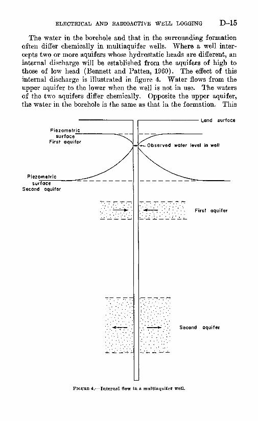
The water in the borehole and that in the surrounding formation often differ chemically in multiaquifer wells. Where a well inter cepts two or more aquifers whose hydrostatic heads are different, an internal discharge will be established from the aquifers of high to those of low head (Bennett and Patten, 1960). The effect of this internal discharge is illustrated in figure 4. Water flows from the upper aquifer to the lower when the well is not in use. The waters of the two aquifers differ chemically. Opposite the upper aquifer, the water in the borehole is the same as that in the formation. This
Piezometricsurface"
First aquiferObserved water level in well
Piezometricsurface
Second aquifer
Land surface
First aquifer
Second aquifer
FIGURE 4. Internal flow in a multiaquifer well.
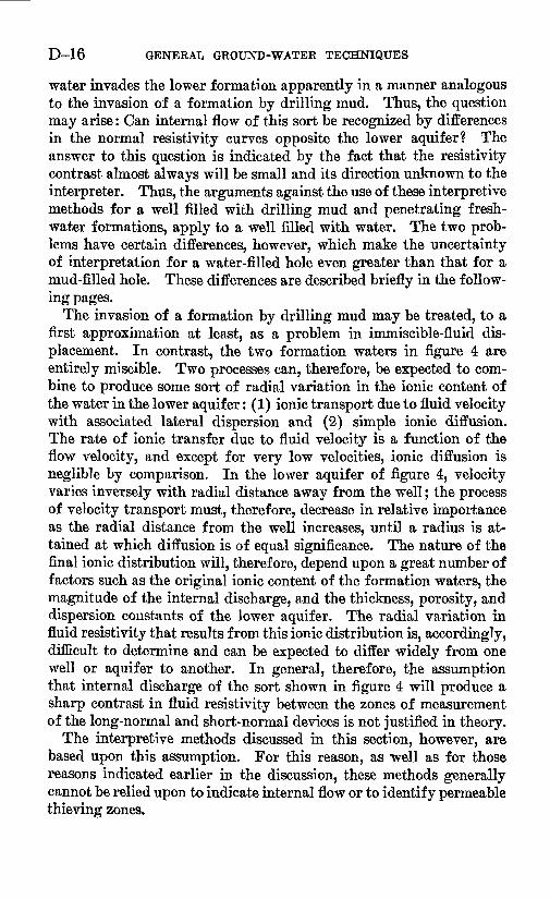
D-16 GENERAL GROUND-WATER TECHNIQUES
water invades the lower formation apparently in a manner analogous to the invasion of a formation by drilling mud. Thus, the question may arise: Can internal flow of this sort be recognized by differences in the normal resistivity curves opposite the lower aquifer? The answer to this question is indicated by the fact that the resistivity contrast almost always will be small and its direction unknown to the interpreter. Thus, the arguments against the use of these interpretive methods for a well filled with drilling mud and penetrating fresh water formations, apply to a well filled with water. The two prob lems have certain differences, however, which make the uncertainty of interpretation for a water-filled hole even greater than that for a mud-filled hole. These differences are described briefly in the follow ing pages.
The invasion of a formation by drilling mud may be treated, to a first approximation at least, as a problem in immiscible-fluid dis placement. In contrast, the two formation waters in figure 4 are entirely miscible. Two processes can, therefore, be expected to com bine to produce some sort of radial variation in the ionic content of the water in the lower aquifer: (1) ionic transport due to fluid velocity with associated lateral dispersion and (2) simple ionic diffusion. The rate of ionic transfer due to fluid velocity is a function of the flow velocity, and except for very low velocities, ionic diffusion is neglible by comparison. In the lower aquifer of figure 4, velocity varies inversely with radial distance away from the well; the process of velocity transport must, therefore, decrease in relative importance as the radial distance from the well increases, until a radius is at tained at which diffusion is of equal significance. The nature of the final ionic distribution will, therefore, depend upon a great number of factors such as the original ionic content of the formation waters, the magnitude of the internal discharge, and the thickness, porosity, and dispersion constants of the lower aquifer. The radial variation in fluid resistivity that results from this ionic distribution is, accordingly, difficult to determine and can be expected to differ widely from one well or aquifer to another. In general, therefore, the assumption that internal discharge of the sort shown in figure 4 will produce a sharp contrast in fluid resistivity between the zones of measurement of the long-normal and short-normal devices is not justified in theory.
The interpretive methods discussed in this section, however, are based upon this assumption. For this reason, as well as for those reasons indicated earlier in the discussion, these methods generally cannot be relied upon to indicate internal flow or to identify permeable thieving zones.
ELECTRICAL AND RADIOACTIVE WELL LOGGING D-17
Certain lithologic conditions can bring about unusual differences between the normal resistivity curves. The authors believe that such conditions often have been mistaken for differences in fluid resis tivity in hydrologic work.
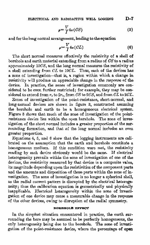
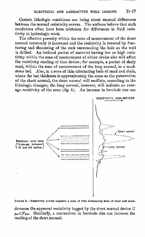
The effective porosity within the zone of measurement of the short normal commonly is increased and the resistivity is lowered by frac turing and shattering of the rock surrounding the hole as the well is drilled. An isolated pocket of material having low or high resis tivity within the zone of measurement of either device also will affect the resistivity reading of that device; for example, a pocket of shaly sand, within the zone of measurement of the long normal, in a sand stone bed. Also, in a zone of thin alternating beds of sand and shale, where the bed thickness is approximately the same as the penetration of the short normal, the short normal will oscillate, according to the lithologic changes; the long normal, however, will indicate an aver age resistivity of the zone (fig. 5). An increase in borehole size can
RESISTIVITY, OHM-METERS
Resistant sand beds /Thickness betweerA V 16 and 64 inches /
-Short normol
Long normal
FIGURE 5. Resistivity curves opposite a zone of thin alternating beds of sand and shale.
decrease the apparent resistivity logged by the short normal device if pm<Fpw Similarly, a contraction in borehole size can increase the reading of the short normal.
D-18 GENERAL GROUND-WATER TECHNIQUES
SUMMARY OF INTERPRETATION OF THE REIjATIVE MAGNITUDE OFNORMAL CURVES
Any interpretation based on the relative magnitudes of the normal curves is hazardous in hydrologic work, because the resistivity con trasts are generally small. Even in oil-reservoir work, where strong resistivity contrasts prevail, the use of the normal curves in this type of interpretation is open to question. It may be noted that advances in instrumentation have provided more reliable ways of employing these interpretive methods in the oil industry. For example, the dif ference in apparent resistivity between a microlog and a laterolog can provide a reliable indication of mud invasion, if a strong resistivity contrast is present. However, these interpretive methods cannot be improved appreciably in ground-water work by the use of such in strumentation, as the strong resistivity contrast is generally lacking.
RELATION OF POROSITY TO FORMATION FACTOR
Empirical relations between porosity and formation factor have been used extensively in the oil industry, and have also been applied frequently to hydrologic problems. A brief discussion of the appli cability of these relations in hydrology will be given in this section.
Archie (1942) first recognized a relation between porosity and formation factor, as a result of experiments on various sands from the Gulf Coast region. Archie restricted the validity of his equation to sandstones ranging from 10 to 40 percent in porosity, and saturated with brine containing from 20,000 to 100,000 milligrams per liter of sodium chloride. A great deal of further experimentation followed Archie's work, and the relation commonly used today is a slight modi fication of the equation he proposed. The modified equation has the form
F=C$- (9)
where <f> is the porosity, and G and m are constants for the formation. Equation 9 is basically empirical in nature; although various theo
retical derivations of the equation have appeared in the literature, all of these are open to question on one ground or another. In these derivations, for example, it is assumed that the effect of the porous medium is purely geometrical that it acts only to decrease the cross sectional area available to the ionic current and to extend the effective length of current path. This assumption is not applicable to rocks containing an appreciable fraction of clay minerals, because these minerals tend to modify the mechanism of conduction, as described in an earlier section. Even if it can be assumed that the rock is free of clay minerals, the theoretical derivations of equation 9 remain open
ELECTRICAL AND RADIOACTIVE WELL LOGGING D-19
to some question. Equation 9 should, therefore, be treated as an empirical relation. For example, the equation should not be applied to a formation until experimental control has established (1) the validity of the equation in the formation and (2) the values of the constants C and m for the formation.
In the oil industry this experimental control is normally established by core analysis. Formation factor and porosity are measured in the laboratory for a number of cores from the formation in question. A plot of log F versus log <£ is then constructed. If the plot is a straight line, the equation is known to apply, and the constants C and m can be obtained from the intercept and slope of the line. A great deal has been published concerning the correction of formation-factor data for the effect of clay minerals, and such corrections are sometimes at tempted in the core analysis procedure if the formation is known to be shaly. This generally involves an increase in the amount of core data which must be analyzed.
Under the conditions prevailing in the oil industry, equation 9 can be a very useful relation. Core analyses from a small group of wells in an oil field can frequently establish the porosity-formation- factor relations for the various strata, and porosity determinations in the remainder of the wells can then be made on the basis of electric logging data alone. It is seldom necessary to apply the relations at any great distance from the region represented in the laboratory con trol, as most oil fields are limited in areal extent.
These conditions, however, are rarely duplicated in hydrologic work. Aquifers are normally much greater than oil fields in areal extent. The amount of laboratory control necessary for the applica tion of equation 9 throughout an aquifer is, therefore, usually greater than that necessary in an oil field operation. The opportunities to obtain core data, however, are normally far fewer in a hydrologic study than in an oil reservoir investigation. In unconsolidated aquifers it is virtually impossible to obtain undisturbed samples for laboratory analysis, and even in consolidated aquifers it is seldom possible to obtain enough cores for adequate control.
Because of the difficulty in obtaining adequate control, there has been a tendency among hyclrologists to make use of equation 9 without such control, using arbitrarily chosen values for G and m. There are three basic assumptions involved whenever this is done: (1) the equation applies to the aquifer, (2) the term G has the particular value chosen, and (3) the term m has the particular value chosen. Each of these assumptions is open to question owing to the empirical nature of equation 9. Used without control, therefore, the equation is at best a method of rough approximation. Results obtained
D-20 GENERAL GROUND-WATER TECHNIQUES
through its use in this manner should be labelled and qualified ac cordingly.
A reliable method of porosity determination in the field, without extensive laboratory control, would obviously be of great importance in hydrology. Such a method may eventually be provided by the neutron-neutron or acoustic-velocity techniques now in use or under development in the oil industry.
RECOGNITION OF SECONDARY POROSITY IN LIMESTONE AND CRYSTALLINE ROCKS
Electric logging in igneous and metamorphic rocks has been stud ied much less intensively than that in sedimentary rocks, because crystalline rocks are rarely penetrated in oil wells. Crystalline rocks constitute some important aquifers, however, and the question natu rally arises as to whether any useful information can be gained from electric logs in such material.
Crystalline rock is similar to dense limestone both hydrologically and electrically, and the principles of log interpretation are essentially the same for aquifers of either type. These principles of interpreta tion are similar to those used in the study of limestone petroleum res ervoirs, but the complex instrumentation commonly used in the oil industry for logging in limestone is seldom used in hydrologic work.
Crystalline rocks are highly impervious hydrologically and highly resistant electrically. Water and ionic charges can move only through fractures in the rock and through the shattered or weathered zones associated with fractures. In other words, the familiar features of secondary porosity in crystalline rocks fractures, joint planes, shat tered fault zones, and associated features are the water-bearing zones of the rocks and are characterized by a relatively low electrical resistivity.
The same principles hold true regarding dense limestone, except that in limestones the origin of the secondary porosity is usually solu tion along fracture zones or bedding planes. These principles can be applied also to a section of dense limestone containing porous sand beds. The sand beds are zones of primary porosity but are hydrolog ically and electrically similar to solution zones in that they are usually permeable and permit ionic conduction. Dense limestone, like crystal line rock, is relatively impervious and highly resistant.
The success or failure of a particular well in crystalline rock or in limestone depends upon the number of permeable zones intercepted by the well and the capacity of each to yield water to the well. In the development of a well field, it is desirable to know the thickness and depths of these zones, as the location of the zones in a few wells
ELECTRICAL AND RADIOACTIVE WELL LOGGING D-21
may aid in the selection of new drilling sites. Similarly, in a study of regional hydrology, the location of permeable zones in several wells may help to outline a regional pattern of occurrence. In a well that penetrates both sedimentary and crystalline material, it may be nec essary to know which is the principal aquifer. Fractures in the crys talline rock indicate that the crystalline rock may be the aquifer; the absence of fractures, on the other hand, definitely establishes the sedi mentary rock as the aquifer.
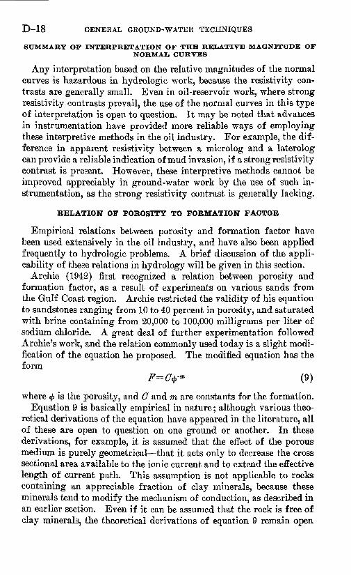
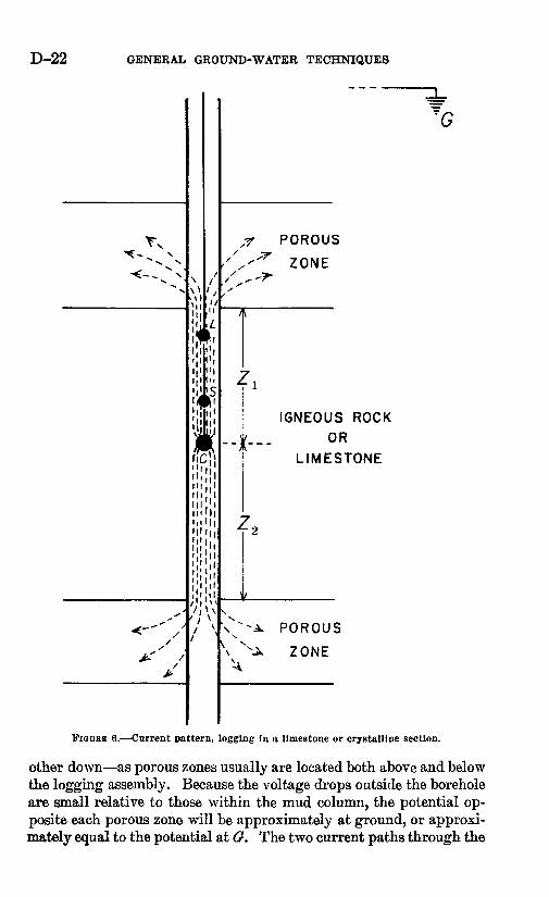
It has been mentioned that there are many similarities between log ging in limestone or crystalline aquifers and logging in limestone oil reservoirs. In the logging of oil wells in limestone, the conventional normal device fails to locate accurately the boundaries of porous zones. These failures are due to the poor conducting qualities of the limestone relative to those of the drilling mud. The logging current tends to con centrate in a linear pattern within the well bore, as shown in figure 6. The extreme deviation from the radial current pattern assumed in the calibration equations prevents determination of true limestone resistiv ity. The response of the logging device indicates the potential drop between the measuring electrode and a reference electrode at some re mote point, however, and a brief analysis of the nature of this potential drop explains some of the difficulties of logging in highly resistive formations. For a more complete treatment of this subject the reader is referred to Schlumberger Well Surveying Corp. (1950).
The current from C follows the borehole until a porous, conductive zone is reached. It then spreads radially through this porous zone; as it does so, the surface area of dense limestone exposed to current pene tration expands rapidly. The logging current thus enters the impervi ous limestone over a wide cross-sectional area, at a low current density, and returns to the ground terminal through the limestone. The log ging circuit, therefore, includes a segment of borehole, the porous zone, a large volume of impervious limestone, and the logging cables. The large cross-sectional area of the limestone causes the total resistance of that segment of the circuit to be effectively zero, in spite of the high resistivity of the material. The flow area begins to expand as soon as the current enters the porous zone, and except for a small region im mediately surrounding the borehole, the resistance of the porous zone also is effectively zero. Thus the voltage drop between a measuring electrode at L and a ground electrode will be controlled more heavily by the resistance of the borehole fluid between L and the porous zone than by the resistance of any material outside the bore.
In practice, the constant logging current leaving the source nor mally will divide into two current paths one up the borehole and the
D-22 GENERAL GROUND-WATER TECHNIQUES
n^»* N
"^~ - S ,
v
^'
<~""' ''
s
4? /
\ /
\" 'll"'ll l|l'
iJi/.i\'('I'' 1!|l M
'(JlS(JBi I 'T'
*iii ii ' iMl 1 1 1
in i1 1 1 ' i
Hi'iii ' i 1 1 1 ' i ' 1 1iii H
ni ii > u1 ii
' /' *\
f \/
X
/s
1
--)
\S
\X
\
.r POROUS
.'* ZONE^-^
\
7
IGNEOUS ROCK
(... OR LIMESTONE
7 -2
t
-± POROUS
XA ZONE
FIGURE 6. Current pattern, logging in a limestone or crystalline section.
other down as porous zones usually are located both above and below the logging assembly. Because the voltage drops outside the borehole are small relative to those within the mud column, the potential op posite each porous zone will be approximately at ground, or approxi mately equal to the potential at G. The two current paths through the
ELECTRICAL AND RADIOACTIVE WELL LOGGING D-23
borehole, thus, may be considered parallel resistances between the current source and ground, and the two currents will be in the ratio
I\ __ RZ __ pBaZzfA _ 2/2 RI
where /t is the current toward the upper porous zone, /2 the current toward the lower porous zone, Zt and Z2 the corresponding distances, and A the borehole area. Thus, the two factors governing the potential drop between L and G the current /i and the resistance of the segment of borehole between L and the upper porous zone both vary with the position of the logging assembly between the two zones.
If the logging assembly is of the design shown in figures 1 and 6, it can be demonstrated that the voltage difference (or the apparent re sistivity) follows a parabolic curve, having a maximum at the mid point of the limestone interval and minima opposite the porous zones. On many normal-resistivity devices, however, one or both of the ter minals D and G (fig. 1) are mounted on the logging cable at some dis tance far enough above L to be considered at infinity in formations of moderate resistivity. In limestone sections, the symmetry of the resistivity parabola will be disrupted if either of these terminals lies between L and the upper porous zone, although the minima opposite the porous zones still will be present.
Whether the terminals D and G are on the cable or at the surface, the porous zone is located approximately by the minimum in the ap parent resistivity; however, its boundaries may not be marked by the relatively sharp resistivity breaks characteristic of a sandstone- shale section. In the oil industry, accurate location of the boundaries of a porous zone is generally necessary, particularly when a well is to be cemented and perforated. This has led to the development of such devices as the "limestone sonde," which are capable of outlining the boundaries of a porous zone with relatively high accuracy.
Devices of this sort would be useful in solving ground-water prob lems in limestone or crystalline rock, but satisfactory logs generally can be obtained with the conventional normal device. This is due partly to the fact that an approximate delineation of the porous zones is satisfactory in solving many ground-water problems and partly to the fact that the borehole often contains fresh water that is more resistive than the drilling mud used in oil wells.
In the above analysis of apparent resistivity in zones of high for mation resistivity, the current was assumed to remain entirely within the borehole, in a linear pattern. This is, of course, an idealization, which can be attained only when the resistivity of the formation isinfinite or, in other words, when the ratio ^^ is zero. Similarly, the
pt
D-24 GENERAL GROUND-WATER TECHNIQUES
radial flow assumed in the calibration equations also is an idealiza tion, which, can be attained only when the above ratio is unity. In ground-water work, the current pattern usually lies somewhere be tween these two extremes, according to the value of the resistivity ratio. Although the ratio always will be low in a water well in lime stone or crystalline rock, it often will be several times greater than in an oil well in limestone, since the resistivity of the borehole fluid in the water well often will be greater. A greater proportion of the logging current will, therefore, penetrate the formation directly. This helps to explain the relatively good quality of the normal curves for many water wells penetrating material of high resistivity, when the borehole fluid is fresh water.
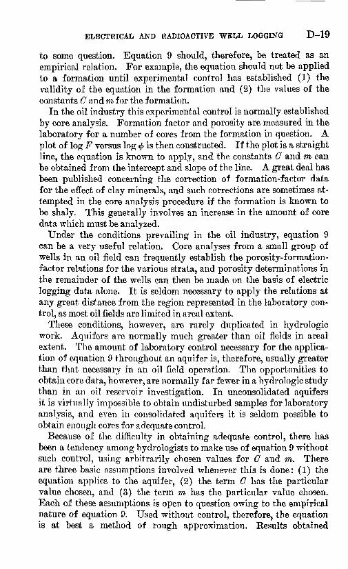
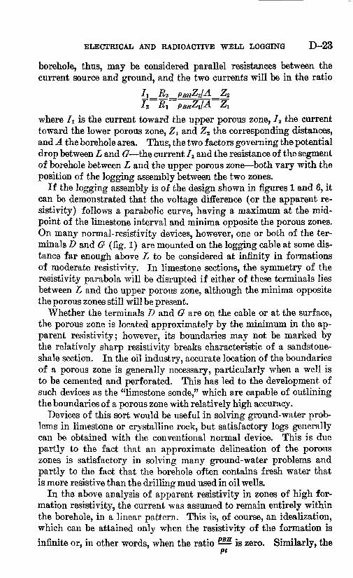
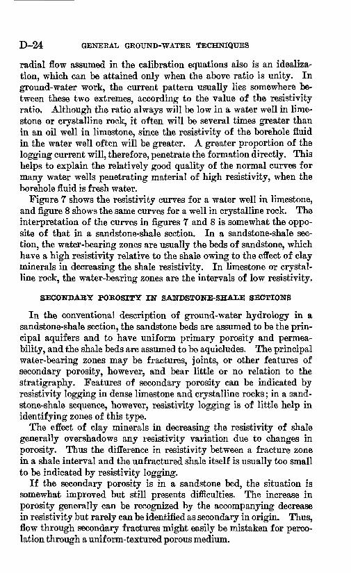
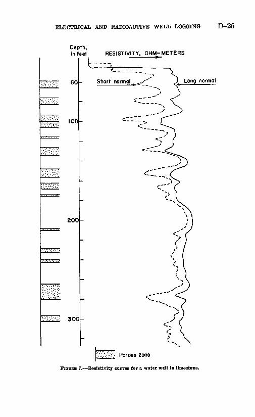
Figure 7 shows the resistivity curves for a water well in limestone, and figure 8 shows the same curves for a well in crystalline rock. The interpretation of the curves in figures 7 and 8 is somewhat the oppo site of that in a sandstone-shale section. In a sandstone-shale sec tion, the water-bearing zones are usually the beds of sandstone, which have a high resistivity relative to the shale owing to the effect of clay minerals in decreasing the shale resistivity. In limestone or crystal line rock, the water-bearing zones are the intervals of low resistivity.
SECONDARY POROSITY IN SANDSTONE-SHALE SECTIONS
In the conventional description of ground-water hydrology in a sandstone-shale section, the sandstone beds are assumed to be the prin cipal aquifers and to have uniform primary porosity and permea bility, and the shale beds are assumed to be aquicludes. The principal water-bearing zones may be fractures, joints, or other features of secondary porosity, however, and bear little or no relation to the stratigraphy. Features of secondary porosity can be indicated by resistivity logging in dense limestone and crystalline rocks; in a sand stone-shale sequence, however, resistivity logging is of little help in identifying zones of this type.
The effect of clay minerals in decreasing the resistivity of shale generally overshadows any resistivity variation due to changes in porosity. Thus the difference in resistivity between a fracture zone in a shale interval and the unf ractured shale itself is usually too small to be indicated by resistivity logging.
If the secondary porosity is in a sandstone bed, the situation is somewhat improved but still presents difficulties. The increase in porosity generally can be recognized by the accompanying decrease in resistivity but rarely can be identified as secondary in origin. Thus, flow through secondary fractures might easily be mistaken for perco lation through a unif orm-textured porous medium.
ELECTRICAL AND RADIOACTIVE WELL LOGGING D-25
Depth,in feet RESISTIVITY, OHI^METERS
60
100
200-
::v::-V.-V:. 300
Long normal
[::'/..'.':'."v Porous zone
FIGURE 7. Resistivity curves for a water well in limestone.
D-26 GENERAL GROUND-WATER TECHNIQUES
Depth, in feet
RESISTIVITY, OHM-METERS
Triassic arkose
_ _ _ _ _ _j'_ _Contact
100
Short normal
Cambrian quartzite
FIGURE 8. Resistivity curves for a water well In crystalline rocks.
These situations illustrate the inadequacy of resistivity logging to supply complete information, even qualitative information, regarding the hydrology of a well. Thus, before the interpretation of resistiv ity data is attempted, all available evidence from other sources, includ ing other types of well logs, should be studied.
SPONTANEOUS-POTENTIAL LOGGING
The spontaneous-potential curve is of great importance to the pe troleum engineer, and it is natural that it should have been adopted in hydrology, especially because spontaneous potentials are related to the movement and chemical quality of the formation water. This method probably exceeds all others, however, in the number and grav ity of the errors that have characterized its application to ground water.
INSTRUMENTATION
The spontaneous-potential logging device is certainly the simplest logging device in use. It consists only of a recording galvanometer
ELECTRICAL AND RADIOACTIVE WELL LOGGING D-27
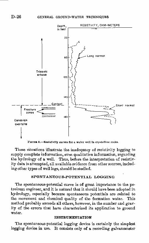
connected between a ground terminal at the surface and a moving electrode on an insulated conductor in the borehole. The galvanome ter measures the potential difference between the earth at the surface and the point in the mud- or water-filled borehole occupied by the moving electrode, and it records this potential difference as a function of depth. The result is a log in which the deflections indicate poten tial differences between points along the axis of the well.
HISTORY
The spontaneous-potential log came into common use shortly after 1927, when potential differences in the borehole between points oppo site sandstone beds and points opposite adjacent shales were recog nized. Deflections on the spontaneous-potential log thus were asso ciated with sandstone-shale contracts, and an excellent method of lithologic correlation was obtained. A further use for the spontane ous-potential log became evident when a theoretical analysis was made relating the magnitude and direction of the spontaneous-potential deflection to the difference in sodium chloride concentration between the fluids of the bore and the formation. This theoretical analysis led to the relation given by Wyllie (1949)
A/S7>=-70.51og10 (10)
in which ASP is the spontaneous-potential deflection, aw is the mean ionic activity, or effective concentration, of sodium chloride in the formation water, and asn is the mean ionic activity of sodium chloride in the borehole fluid.
By use of this equation, aw can be calculated from the measured spontaneous-potential deflection from shale base and the known ac tivity of the drilling mud, if the temperature also is known. The sodium chloride concentration of the formation water then can be obtained from graphs of activity versus concentration. Equation 10 has become popular with hydrologists and has been used to determine the concentration of formation waters in both mud-filled and water- filled boreholes. The question of the applicability of the equation to ground- water problems is, therefore, of considerable importance; it can be analyzed by a review of spontaneous-potential theory and by a consideration of some of the assumptions implicit in the deriva tion of equation 10.
ANALYSIS OF QUANTITATIVE INTERPRETATION
If two solutions having different concentrations of the same mono- valent salt are brought into contact, ions will be diffused toward the
D-28 GENERAL GROUND-WATER TECHNIQUES
solution of lower activity. It is assumed that the fluids are static and that ions move only as a result of diffusion. Each ion carries a charge, either positive or negative, which is equal in magnitude to the charge of an electron. If equal numbers of positive and negative ions diffuse across a given boundary in a unit time, there will be no net transport of charge across the boundary. In general, however, the positive and negative ions will not diffuse at equal rates, and there will be a net flow of charge across the boundary. The tendency of the anions and cations to diffuse at different rates thus establishes a potential, or electromotive force, in a direction that depends upon the sign of the excess ionic charge crossing the boundary.
The difference in the rates of diffusion arises from a difference in the mobilities of the two ionic species and tends, in the absence of a complete circuit, to produce a separation of positive and negative charge. The resultant electrostatic forces eventually oppose any fur ther net movement of charge and, thus, eliminate any current. If, however, a circuit is completed between the high- and low-activity solutions through a conducting path external to the liquid junction, a current will be established, because the excess charge diffusing into the low-activity region will be balanced by an inflow of opposite charge through the external branch of the circuit.
The components of a liquid junction need not be pure solutions of the same monovalent salt, as in the example discussed above. More generally, the potential represents the net effect of the diffusion of several ionic species, each in the direction of decrease in its own activity.
In a liquid junction between two pure solutions of sodium chloride, the number of chloride ions diffusing across an area in a unit time exceeds the number of sodium ions approximately in the ratio of six to four, owing to the greater mobility of the chloride ion. Thus, the net transfer of charge in the direction of the low-activity solution is negative, which corresponds to a current and emf (electromotive force) directed toward the high activity solution.
The transport number of an ion in a liquid-junction problem is defined as the ratio of the quantity of charge carried by this type of ion across a given plane in a unit time to the total charge moved across the plane in both directions in a unit time. The transport number of an ion depends upon the concentration, mobility, and valence of that ion, and the concentrations, mobilities, and valences of all other ions present. The sum of the transport numbers of all the ions in any diffusion problem is unity. In a liquid-junction involving several ionic species, the transport number of any given species is extremely difficult to determine and must, in general, be treated as an unknown
ELECTRICAL AND RADIOACTIVE WELL LOGGING D-29
function. This makes a mathematical analysis of such a liquid junc tion difficult, if not impossible.
The determination of transport numbers in liquid junction between two pure sodium chloride solutions, however, is straightforward. Each solution contains the same number of cations as anions, and each ion carries a single positive or negative charge. Neglecting transport by the solvent, all charge that is not carried by the anion must be carried by the cation. The transport numbers, thus, become functions only of the mobilities of the two species. The transport number of the chlo ride ion is approximately 0.6, and that of the sodium ion is 0.4. Al though these transport numbers vary slightly with the total sodium chloride concentrations, this variation can be neglected without intro ducing serious errors, as far as electrical well logging is concerned.
THE GENERAL, LIQUID-JUNCTION EQUATION
The general equation derived by Glasstone (1951) for a liquid- junction potential between two solutions is
p'T'___ 1 f*II
F i Zijj
in which Zn is the valence, ti the transport number, and at the activity of the ith ionic species; R is the universal gas constant, T is the abso lute temperature, and F is the Faraday. Each term in the summation represents the contribution made to the net emf by the diffusion of a single ionic species, and the summation is taken over all the species in the problem. Thus, if only a single species of ion were diffused, the equation would simplify to
'//(12)
where Z^ £15 and a^. now refer to the species of ion present.The integration in equation 12 and each integration in equation 11
are carried out over the range of activity of a particular ionic species. The limits / and // refer to the log of the activity of the species at the two endpoints of the problem, between which the measurement of emf is made. An infinitesimal difference in the activity of a particular ionic species produces a difference of potential according to the relation
ac.=-f^\/JfT\ 1( \ tid In «!
Integration sums these changes over the entire range present to obtain the total emf that is due to diffusion of the species 1.
D-30 GENERAL GROUND-WATER TECHNIQUES
The sign of the emf of equation 12, or of the individual terms in the summation of equation 11, is controlled by the sign of the valence, in accordance with the principle that positive and negative ions diffusing in the same direction produce emf 's of opposite sign. The direction of diffusion of each species also controls the sign ; this is expressed in the equations by the relative magnitudes of the limits / and //.
The denominator, FZ^ on the right side of the equations is the charge carried by 1 mole of the diffusing species ; the potential change is a measure of the energy expended per unit charge in the diffusion process.
EQUATION FOB DIRECT JUNCTION BETWEEN TWO SODIUM CHLORIDESOLUTIONS
The integrals in equation 11 usually are difficult to evaluate, as the transport numbers of the various species are usually unknown func tions. Equation 11 assumes a greatly simplified form, however, when applied to a liquid junction between two pure sodium chloride solu tions. The summation includes only two ions, and because the trans port numbers are effectively constant, they may be taken outside the integrals, giving
n 06= FLTT, <"B <*"+(±I
or
RT TO 4 CE= FLTTJ,
[~
L
=~- 0.4 InNa-/
Each of the individual activities of the sodium and chloride ions, <zNa and flci, may be replaced by the mean ionic activity of the sodium chloride, am. After making these substitutions and carrying out the integrations, equation 13 simplifies to
=-r (-0.2) log ^=+11.5 log %=& (14) r dm-i a>m-i
at 25 °C, when E is expressed in millivolts and common logarithms are used in place of the natural logarithms.
JUNCTION OF SODIUM CHLORIDE SOLUTIONS THROUGH AN ION-SELECTIVE MEMBRANE
If the two sodium chloride solutions, rather than being brought into direct contact, are brought into contact through a porous membrane through which only positive ions can pass, the situation is considerably altered. The anions are prevented from crossing the membrane, and, in the absence of an external circuit branch between the two solutions, electrostatic attraction will prevent any sustained transfer of charge
ELECTRICAL AND RADIOACTIVE WELL LOGGING D-31
through the membrane by the diffusion of cations. Just as in a direct liquid junction, however, a flow of charge will begin as soon as a com plete circuit is available that is, as soon as some means is available to balance the excess positive charge appearing on one side of the membrane and the excess negative charge remaining on the other. The flow of charge through the membrane will consist entirely of the movement of positive ions and can be expected to have a different value than that of a flow maintained by a difference in the normal rates of diffusion of the positive and negative ions. The sodium ion may be assigned a transport number of 1, and the chloride ion a transport number of 0, in accordance with the definition of transport number. The potential, or emf , maintained in the separation of the two solu tions by the membrane then can be calculated by applying equation 11 ; that is,
7?T
RTT 1 C" 1 Cn ~\ = Y I q-^ I (l)cnnaNa+ I (0)dlnaCi\
Again using mean ionic activity in place of aNa, equation 15 may be written as
j= j=r In F
which becomes
at 25°C, using common logs and the units employed in equation 14. Thus the emf is several times larger than that of a direct liquid junc tion and is oppositely directed.
HOLE OF SHALE AS AN ION-SELECTIVE MEMBRANE
Many investigations have been made into the role of clay and shale in controlling the spontaneous-potential log. Various physical and mathematical models have been used to describe the processes by which clay minerals control the diffusion of ions. The reader is referred to the work of McCardell, Winsauer, and Williams (1953), Wyllie (1955), and DeWitte (1955) for detailed analyses of the interaction of ions with clay particles. The overall effect of shale is to block
D-32 GENERAL GROUND-WATER TECHNIQUES
the diffusion of negative ions in the manner of an ion-selective mem brane. The action of the shale as an ion-selective membrane follows from the same basic clay properties that cause the low resistivity of shale.
If two sodium chloride solutions are brought into contact through a segment of shale, transfer of negative ions through the shale will not be possible, and a potential measurement between the solutions will show the result predicted by equation 16. This holds true even if the shale is saturated with a solution of different activity from either of the two solutions that it separates. The net potential between the end solutions is the algebraic sum of the two potentials (each of which follows the form of equation 16) between the solution within the shale and each end solution. Thus, if the activity of the cation in the solu tion within the shale is a Na-s, the potential between the end solutions would be
"3- lm ^Na-// | / RT\ j= =- In - H w } In* %Ta-S \ $ /
R T
, QNa-77 "'*
am-JI
The concentration of the solution within the shale does not affect the potential between the solutions separated by the shale; in calcu lating the spontaneous-potential, the shale may be treated simply as an ion-selective membrane.
LIQUID-JUNCTION POTENTIALS IN AN OIL WELL
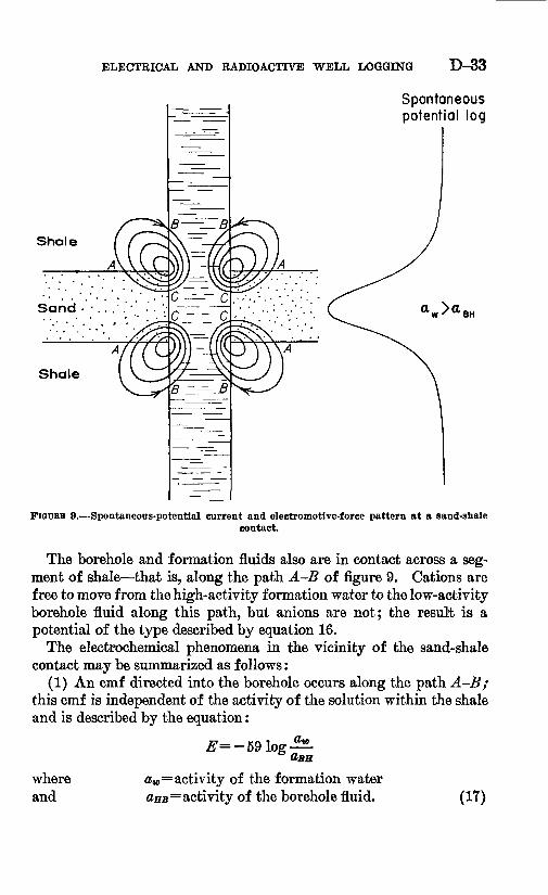
In the drilling of an oil well, liquid- junction potentials arise from chemical differences between borehole and formation fluids. Figure 9 illustrates the electrochemical reactions at the contact of a bed of sand and beds of shale in the borehole. Both the borehole fluid and the formation water in the sand bed are assumed to be pure sodium chloride solutions of different activities. A direct liquid junction will exist at the borehole wall opposite the sand bed. The formation water generally will have the higher activity, and the net charge moving into the borehole will be negative, owing to the fact that the chloride ion is more mobile than the sodium ion.
ELECTRICAL AND RADIOACTIVE WELL LOGGING D-33
Spontaneous potential log
Shale
Shale
FIGUHE 9. Spontaneous-potential current and electromotive-force pattern at a sand-shalecontact.
The borehole and formation fluids also are in contact across a seg ment of shale that is, along the path A-B of figure 9. Cations are free to move from the high-activity formation water to the low-activity borehole fluid along this path, but anions are not; the result is a potential of the type described by equation 16.
The electrochemical phenomena in the vicinity of the sand-shale contact may be summarized as follows:
(1) An emf directed into the borehole occurs along the path A-B; this emf is independent of the activity of the solution within the shale and is described by the equation:
where and
aw = activity of the formation water activity of the borehole fluid. (17)
D-34 GENERAL GROUND-WATER TECHNIQUES
(2) An emf directed away from the borehole occurs opposite the sand at G. This emf is described by the equation :
#=11.5 log 2*- (18)
(3) A complete circuit is established: the path A-B forms the ex ternal conducting branch for the liquid junction at 0 '; the sandstone and borehole form the external conducting branch for the "mem brane" emf between A and B.
(4) As a complete circuit is present, a movement of charge occurs. Positive ions diffuse into the borehole through the shale, and both positive and negative ions diffuse into the bore through the sand, with the negative ions here diffusing at a higher rate. The resultant sepa ration of charge sets up a field that causes positive ions to move through the borehole from B to O and negative ions to move from C to Z?. Thus, the diffusion of ions into the borehole produces a current, or circulation of positive charge, in the direction of the arrows in figure 9.
(5) This circulation of charge occurs at both contacts of the sand stone bed and is such that the movement of positive charge in the borehole is from shale to sand, when the water in the sand is the high- activity solution.
Equations 17 and 18 are derived from electrochemical principles, and the signs in these equations, therefore, follow electrochemical conventions. The opposite signs of emf indicate that one is directed from the high-activity to the low-activity solution, and the other is directed from the low-activity to the high-activity solution. In order to deal with a circuit such as that formed by the spontaneous potential current loop in figure 9, however, a new sign convention must be chosen in which emf is taken as positive or negative, according to its direction around the current loop. Each emf is in the same direction in the spontaneous-potential current loop ; they are, therefore, both given the same sign, taken as negative, in the logging equations. Where the borehole fluid is higher in activity than the formation fluid, the direc tion of each emf will be reversed, as will the direction of the spontane ous-potential current.
RELATION OF THE SPONTANEOUS-POTENTIAL MEASUREMENT TO THE THEORETICAL ELECTROMOTIVE FORCE
The three-dimensional circuit at the sandstone-shale contact in figure 9 may be analyzed using the loop rule of Kirchoff, which states that the algebraic sum of the emf's around a circuit loop is equal to the
ELECTRICAL AND RADIOACTIVE WELL LOGGING D-35
algebraic sum of the IR drops around the loop. In the circuit of figure 9, the algebraic sum of the emf ' s is
#=-59 log -^-11.5 log -2s 70.5 logQ>BH
Assuming that the relationsk& =
Pu,and
PBH
holds true, in which pw and PBH are the resistivities of the two fluids and k is a constant, the sum of the emf 's may be expressed as
#=-70.5 logPio
The circuit loop may be divided into three sections, considered as resistances in series. The total logging current remains constant through each segment, and the voltage drop across any segment is given by the product of this current and the total resistance of that segment. Denoting the effective resistance of the sand to the spon taneous-potential current as TJsg, that of the shale as RSa, and that of the borehole as Ran, Kirchoff's law may be written for the problem as
E= -70.5 log =I8PRss+ISPRSIt+ISPRBH (19)Pm
Geometrically, the spontaneous-potential current could assume many patterns of flow through the formations and borehole. The current always will distribute itself, however, in the pattern for which the total resistance of the circuit is a minimum. If the true forma tion resistivities are not high relative to the resistivity of the borehole fluid, the resistance of the borehole, RBH^ will constitute the major part of the total resistance in this current pattern. This follows from the fact that the current is free to spread over a considerable area within the formations, whereas it is constrained to a small area as it passes through the borehole. The indefinite geometry involved makes calculation of the relative values of Rn^ -#ss, and Ran ex tremely difficult.
Equation 10 is based upon the assumption that the term RBn consti tutes the major part of the spontaneous-potential circuit resistance, so that the terms IspRsH and IspRss can be dropped from equation 19.
D-36 GENERAL GROUND-WATER TECHNIQUES
The spontaneous-potential device actually measures the potential dif ference between points along the well axis. According to Ohm's law, the potential difference between two points is equal to the IB drop between the points. Thus, the spontaneous-potential deflection actu ally measures the quantity ISP^BH of equation 19. Equation 10 is obtained from equation 19 by neglecting the terms IspRss, and lapRsH, and substituting A/S73 for ISP^BH-
OBJECTIONS TO QUANTITATIVE INTERPRETATION FOR WATERWELLS
The theoretical analysis by which equation 10 is established as the basis of quantitative spontaneous-potential interpretation involves several assumptions, which are summarized and discussed briefly here.
It was assumed, in the first place, that both the formation water and the borehole fluid were pure sodium chloride solutions. Formation waters penetrated by oil wells frequently contain sodium chloride in far greater concentration than any other salt. This is not generally true, however, in water wells. The concentrations of all ions are usu ally low, both in the formation and in the borehole, and sodium chloride is seldom in strong predominance. Frequently such ions as calcium, potassium, sulf ate, or carbonate are of equal or greater con centration. Further, the ionic contents of the formation water and the borehole fluid sometimes differ in a complex manner, so that cer tain ions predominate in the borehole and others predominate in the formation. Obviously the application of equation 10 to such situa tions will lead to erroneous results. The appropriate relation is equation 11, but the number of unknown functions and variables makes quantitative analysis by this equation impossible.
Another assumption in the analysis is that the shale behaves as an ideal ion-selective membrane and that the sand has no ion-sieving properties whatsoever. This assumption is apparently acceptable if the shale is free of sand and the sand is free of clay minerals. Other wise, the result will be an emf different from that predicted by equa tion 19.
The effects of ions other than sodium and chloride, as well as the effects of nonideality of the sand or shale, have received considerable attention in the literature of the oil industry. Such corrections as have been devised for these effects, however, generally require a degree of laboratory control that is not available to the hyolrologist.
Finally, it was assumed that the resistance of the borehole (Rao} in the spontaneous-potential circuit was much greater than the combined effective resistance of sandstone and shale (Bsa+Rao}' This as sumption is generally valid if the true formation resistivities are not
ELECTRICAL AND RADIOACTIVE WELL LOGGING D-37
high relative to the resistivity of the borehole fluid. In the oil in dustry, where the sandstones are saturated with a low-resistivity brine, this condition is usually met ; in hydrologic work, the true resistivity of the sand (pt) is normally many times that of the borehole fluid, and the assumption that
is, therefore, open to considerable doubt, in spite of the restricted area of the borehole.
Thus, there are several points upon which the conditions in a typical water well can be expected to deviate from the conditions assumed in the derivation of equation 10, and the hydrologist will not generally have any means of controlling or correcting for these deviations. Equation 10, therefore, generally cannot be expected to give valid results. Its use in a hydrologic investigation is certain to produce a great deal of erroneous data, regardless of whether the wells involved contain drilling mud or water as their borehole fluid.
INTERAQUIFER FLOW
The invasion of one aquifer by water from another may establish a difference between borehole fluid and formation fluid, resulting in a spontaneous-potential reading. This invasion also presumably will establish some sort of radial concentration distribution in the thieving aquifer, which, in turn, will have an effect upon the spontaneous- potential deflection opposite that aquifer. This effect would be dif ficult to evaluate even if the form of the concentration function were known, but because the form of this function is generally not known, the effect becomes virtually impossible to evaluate. If the concen tration remains nearly that of the invading water for a considerable radius into the thieving aquifer, the effect may simply be to remove the diffusion process from the vicinity of the borehole, thus eliminat ing any spontaneous-potential current in the borehole. The possi bility of this sort of interaquifer flow further complicates the question of quantitative spontaneous-potential interpretation in ground-water studies. On the other hand, the spontaneous-potential deflections can serve as a preliminary indication of the existence of internal circula tion. This applies not only to the electrochemical potentials described above, but also to the streaming potentials that may accompany the internal flow, and which are discussed more fully in the following section. Whenever a large spontaneous potential is recorded in a water-filled borehole, therefore, it is advisable to log the well by flow- meter or to employ some flow-tracing technique.
D-38 GENERAL GROUND-WATER TECHNIQUES
STREAMING POTENTIALS
Small potentials, generally termed streaming potentials, are set up when an electrolyte flows through a porous solid. Such potentials have received some attention in the oil industry, on the theory that they may result from the invasion of a formation by drilling mud and may, thus, contribute to the spontaneous-potential reading. It is possible that they occur in some water wells.
On the basis of theory, streaming potentials should be proportional to the pressure differential causing the flow and inversely propor tional to the conductivity and viscosity of the electrolyte. Kozary (1948) indicates, however, that streaming potentials in wells cannot be predicted by equations derived from theory. The common prac tice in oil reservoir work is to assume that streaming potentials are negligible in comparison to the electrochemical potential. This as sumption appears to be acceptable in view of the agreement between the observed spontaneous potential and the calculated electrochemical potential in oil wells for wliich an independent method of determining aw is available.
A comparison of streaming potential between oil wells and water wells is difficult to make. If, in a water well, the borehole fluid is water and the flow is actually an interaquifer circulation, the pressure differentials will generally be smaller than in a deep oil well. How ever, the conductivity and viscosity of the water will usually also be smaller than those of drilling mud, and the net effect on the streaming potential will be difficult to predict, even on a theoretical basis. If the borehole fluid is drilling mud, the pressure differentials should generally be smaller than in deep oil wells, and this should tend theo retically to make the streaming potentials smaller. Whether the bore hole contains water or mud, however, the electrochemical potentials in most water wells are smaller than those in oil wells. This tends to make the streaming potential relatively more significant, and fur ther contributes to the uncertainty of quantitative spontaneous-poten tial interpretation.
ZONES CONTAINING HIGHLY MINERALIZED WATER
The qualitative recognition of zones containing highly mineralized water is an important aspect of interpretation of spontaneous poten tial. The spontaneous-potential device is particularly valuable in this respect in mud-filled boreholes. In water-filled boreholes, recogni tion of the highly mineralized zones is possible as long as the borehole contains water that is chemically different from that in the zone in question.
ELECTRICAL AND RADIOACTIVE WELL LOGGING D-39
AETIFICIALLY INDUCED SPONTANEOUS-POTENTIAL DEFLECTIONS
A flat and featureless spontaneous-potential log generally indicates that the ion content between the water of the several formations penetrated by the borehole and the borehole fluid opposite the forma tions is only slightly different. In these circumstances, a spontaneous- potential log suitable for lithologic interpretation can be obtained by increasing the salinity of borehole fluid. The borehole fluid, thus, becomes a solution of higher activity than the formation waters, and positive spontaneous-potential deflections should result opposite each sandstone. The potentials observed will be due largely to the diffusion of sodium chloride and should obey equation 19. The term Run, how ever, will be decreased, because the resistivity of the borehole fluid is lowered by the addition of the sodium chloride. Therefore, the as sumption that Ras and Ran are negligible, compared to RSH becomes less tenable than ever, and the use of equation 10 is still unreliable.
ABNOEMAL SPONTANEOUS-POTENTIAL DEFLECTIONS
Occasionally, the spontaneous-potential log may exhibit charac teristics which do not lend themselves to any explanation in terms of liquid junction or streaming potentials. A spontaneous-potential de flection always measures an IR drop in the borehole indicating that ions are moving through the borehole in such a way as to cause a net transfer of positive charge in the direction of more negative potential. No set rules of interpretation for abnormal spontaneous-potential data can be based upon this fact; however, it may sometimes be possible to assign some reason for the ionic movements indicated by an abnormal spontaneous-potential log, and, thus to increase understanding of the hydrology or geology of the well. In any interpretation of this sort, full advantage should be taken of evidence from other logs and other sources of information concerning the well.
Large electrical installations in the immediate vicinity of a well may often cause a spurious response on the spontaneous-potential log.
SUMMARY OF SPONTANEOUS-POTENTIAL LOGGING
The spontaneous-potential log is a valuable qualitative method in ground-water studies. It has great value as a means of lithologic cor relation, and can sometimes aid in the identification of internal flow, or in the location of zones of highly mineralized water. The assump tions involved in quantitative interpretation of spontaneous potential, however, are seldom satisfied in ground-water work. The use of the method as a quantitative tool is, therefore, likely to produce erroneous results.
D-40 GENERAL GROUND-WATER TECHNIQUES
FLUID-CONDUCTIVITY LOGGING
The fluid-conductivity log is generally of somewhat greater import ance to the hydrologist than it is to the petroleum engineer. Its role in the oil industry has been chiefly to serve as a check on the drilling mud, where the mud conductivity is required in the quantitative interpre tation of other logs. In hydrology, on the other hand, the fluid- conductivity log of a water-filled borehole often can give a general indication of water quality and can sometimes provide information on the hydraulics of a well.
Some instruments presently available record the conductivity of the borehole fluid, and other record its resistivity. The discussion pre sented here will be worded in terms of fluid conductivity.
FACTORS CONTROLLING CONDUCTIVITY
The conductivity of the water in the well at a given depth depends upon the concentrations, mobilities, and valences of the ions in the water at that depth. It is, therefore, controlled partly by the pro cesses of ionic diffusion and dispersion and ion transport by moving fluids. These processes are frequently at work both within the well bore and in the formations surrounding the hole. They will generally proceed at different rates and in different manners in these two re gions. The ionic content at a given point in the water-filled borehole, under equilibrium conditions, represents a balance of the various processes in effect at that point.
INTERPRETATION OF FLUID-CONDUCTIVITY LOGGING IN A SINGLE-AQUIFER WELL
With reference to fluid-conductivity logging, water wells can be divided into two groups those that penetrate, wholly or partly, a single aquifer, and those that penetrate several aquifers separated by reason ably effective aquicludes. In a well penetrating a single aquifer, the conductivity of the water in the borehole generally will be the same as that of the water in the aquifer, assuming that this conductivity is uni form throughout the aquifer. If ionic content and, therefore, conduc tivity differ at various depths in the aquifer, the effect will be shown on the conductivity log. However, this variation on the log may have a different form from that in the formation, because vertical ionic diffusion may be proceeding at a different rate in the borehole than in the aquifer.
The interpretation of fluid-conductivity data for wells penetrating a single aquifer is controlled by the following principles: If the log shows no gradient, the conductivity of the water in the aquifer is
ELECTRICAL AND RADIOACTIVE WELL LOGGING D-41
probably the same from top to bottom and is equal to the conductivity shown on the log; if the log displays a gradient, the conductivity of the water in the aquifier differs from top to bottom, although perhaps not in exactly the same way as does the water in the borehole. Never theless, the conductivity range observed in the borehole usually gives an approximate idea of the range in the aquifer.
Conductivity, in itself, is of secondary interest to the hydrologist; in a single-aquifier well it is valuable principally because it provides some idea of the chemical quality of the water. There is no general theoretical method by which the types and concentrations of ions in a solution can be determined from conductivity data alone. Never theless, experience in a particular area or with a particular acquifier will often enable the log interpreter to estimate water quality from the conductivity log, and to decide whether a laboratory analysis is necessary.
INTEBPBETATION OP FLUID-CONDUCTIVITY LOGGING IN A MULTIAQUIFEE WELL
The fluid-conductivity log in a multiaquifer well is controlled largely by ionic transport by moving fluid. The interstitial waters of the various aquifers usually differ in conductivity, and the aquifers usually have different hydrostatic heads, so that internal flow pre vails in the well. Some of the characteristics of internal flow have been discussed in previous sections; in this section, the effects of in ternal flow on the fluid-conductivity log are considered.
Figure 10 shows a three-aquifier well in which the lower and middle aquifiers are yielding while the upper aquifier is thieving. The fluid- conductivity log of the well is also shown. The conductivity of the water in the lower aquifer will be denoted CL, that of the water in the middle aquifer CM, and that of the water native to the uppermost aquifer GU. It will be assumed that CL>CM>CU> It also will be assumed that the velocity within the well bore, at all points between the bottom of the lower aquifer and the top of the upper aquifer, is great enough so that the effect of ionic diffusion is negligible by comparison.
The interval between the bottom of the lower aquifer and the bottom of the middle aquifer is occupied by the water of the lower-most aquifer, which has a constant conductivity, CL. In the interval op posite the middle aquifer, the conductivity changes gradually from GL to a value between CL and CM as the flow in the bore is gradually increased by the discharge from the middle aquifer. The final con ductivity of the mixture depends to a certain extent upon the relative proportions of the discharge from each aquifer. It is difficult to de-
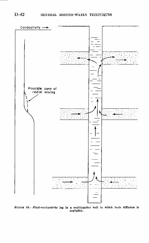
D-42 GENERAL GROUND-WATER TECHNIQUES
Conductivity
Possible zone of radial mixing
FIGURE 10. Fluid-conductivity log in a multiaquifler well in which ionic diffusion isnegligible.
ELECTRICAL AND RADIOACTIVE WELL LOGGING D-43
termine the exact nature of this dependence, however, because the effects of interionic forces may be different in the mixture than in either component solution. In any event, a conductivity gradient will exist opposite the middle aquifer. If mixing occurs instantaneously as the water of this aquifer enters the borehole (so that conductivity is nearly constant radially across the well at any given depth), the con ductivity log will show a constant reading in the interval between the middle and uppermost aquifers.
If mixing is not instantaneous, a zone of mixing will extend above the upper contact of the middle aquifer and will be characterized by variation in ionic content both radially, across the borehole, and ver tically. The process of radial diffusion within the well bore will cause conductivity along the well axis to vary with depth within this zone of mixing. The situation will be further complicated if velocity as well as ionic content varies radially across the borehole. It is prac tically useless to attempt to analyze the net effect of these processes upon the fluid-conductivity log because the logging instrument does not normally measure the conductivity along the well axis. Most instruments are designed to measure an average conductivity involv ing as much of the hole cross section as possible; it is usually impos sible, moreover, to know whether the instrument is centered or hang ing against the wall at a given depth. About all that can be said is that if mixing is not instantaneous opposite the middle aquifer, some form of conductivity gradient or perhaps some slightly erratic conductivity variation may be observed on the log for a short distance above the aquifer.
A constant conductivity should be observed on the log once the zone of mixing has been passed. This conductivity will prevail at least to the top of the uppermost aquifer, and it probably will hold in the zone above this level, because diffusion from the stagnant water of this zone would tend to remove any chemical differences.
It is the authors' belief, as outlined in the discussion of resistivity logging, that the decreasing radial-flow velocity within the thieving formation causes ion transport by moving fluid to decline in impor tance relative to ionic diffusion. The balance of these two processes tinder equilibrium conditions should, therefore, create a radial con centration distribution within the thieving aquifer, by which con ductivity ranges from that of the mixture in the well bore to that of the water native to the upper aquifer. The important consideration in fluid-conductivity interpretation is that within the well bore oppo site the thieving zone velocity is high, diffusion is negligible, and the concentration is that of the mixture from the lower aquifers.
D-44 GENERAL GROUND-WATER TECHNIQUES
The reader may verify, by an analysis similar to that given for the situation assumed above, that the conductivity log would have a simi lar form if the flow were downward that is, if the lowermost aquifer were the thieving zone. The only difference in form that might occur would be that the mixing zone, if present at all, would extend down ward from the lower contact of the middle aquifer.
The difficulties of stating a definite set of interpretive principles under these conditions are obvious. The interpreter can be relatively certain that there is measurable internal flow because there are no concentration gradients except in the vicinity of one of the aquifers. This, however, is about as far as reliable interpretation can go, on the basis of the conventional conductivity log alone.
Information on the direction and the magnitude of the internal flow can be obtained by releasing a small amount of brine in the well and tracing its movements with the conductivity device. The brine may be released at any desired depth by breaking a suspended con tainer or by siphoning through a hose from a container at the surface. Velocity measurements can be made by timing the traverse of the brine between two points in the well. If flowmeter equipment is avail able, such tracing experiments are unnecessary.
When the direction of the internal flow is established, the conductiv ity log may be evaluated properly. In the example given in this sec tion, once the flow direction is known, the conductivity in the region between the lower and middle aquifers is established as that of the water native to the lower aquifer. A rough idea of the quality of this water is, thus, obtained. It is established also that the water of the middle aquifer is less conductive and, therefore, probably of better quality than that of the lowermost aquifer. If the discharge of each aquifer to the well has been measured, a better idea of the order of magnitude of On is possible, because the conductivity of the mixture is governed by the proportions as well as the conductivities of the com ponent solutions. Here again, however, no calculation is proposed, because the effects of interionic forces in the mixture may be different than that in either component.
Finally, the flow-tracing data established that the conductivity log gives no information about the water native to the uppermost aquifer. The only way in which information on this water can be obtained is by logging during pumping and only after pumping has been in progress long enough to produce a drawdown sufficient to cause the thieving zone to yield water. Even here, the only information provided is that the water of this aquifer is less conductive and, therefore, probably fresher than the mixture from the lower two aquifers. Effects of this sort are of interest in many problems not involving well logging; for
ELECTRICAL AND RADIOACTIVE WELL LOGGING D-45
example, the quality of the water discharge by a well often changes during the course of pumping. This may be caused by the reversal of a thieving process, as outlined here.
Given a set of circumstances, a fluid-conductivity log is easy to inter pret ; it is difficult, however, to phrase a set of interpretive principles general enough to cover all of the possible situations in a problem in volving internal flow. However, if the log shows extensive intervals of constant conductivity and conductivity gradients only in the vicin ity of certain aquifers, measurable internal flow usually is indicated, and brine-tracing or flowmetering experiments should be run to estab lish the direction and magnitude of the flow. The conductivity log then can be analyzed in the light of this new information in the manner indicated in the example.
GAMMA-RAY LOGGING
Interpretive procedures for utilizing gamma-ray logs have, for the most part, been restricted to qualitative identification of lithology and formational contacts. In this capacity the gamma-ray log is a valu able supplemental tool to resistivity methods, as it is normally un affected by adverse borehole conditions such as those caused by oil-base or highly mineralized drilling fluids. It should be noted, however, that drilling fluids containing radioactive minerals can have a serious effect on the gamma-ray log.
Various attempts have taen made to develop more quantitative tech niques for using gamma-ray log information. Many of these have been attempts to relate the gamma intensity of a particular formation to its clay content or sand-shale ratio.
GENERAL DISCUSSION OF RADIATION AND GAMMA-RAY-LOGGINGINSTRUMENTATION
Gamma radiation originates in the spontaneous disintegration of atomic nuclei of various radioactive elements. Other forms of radia tion, alpha and beta rays and neutron emission, are of no direct inter est in gamma logging, as their effects are not detected by gamma- sensitive instruments.
Eadiation intensity at any particular point in a well depends on several factors, the most obvious of which is the concentration and activity of radioactive elements disseminated in the rocks around the borehole. Of the many radioactive isotopes in nature, only a few are concentrated to the extent that their radiation may be measured by ordinary means. Gamma radiation from uranium, thorium, and their daughter products, and an isotope of potassium (atomic weight 40) constitutes virtually all the radiation usually measured in the
D-46 GENERAL GROUND-WATER TECHNIQUES
borehole, although some other elements have radioactive isotopes that occur naturally. The relative abundance of the radioactive isotopes of the three above-named elements in sedimentary rocks is small; for example, the abundance of K40 in potassium is 0.011 percent, and only 10 percent of the disintegrating atoms of this isotope emit gamma radiation (Faul, 1954). The radiation from uranium and thorium also originates largely from particular isotopes, but in this discussion the element will be referred to rather than the specific radioactive isotope.
The radioisotopes of uranium, thorium, and potassium are not uni formly radioactive, as they decay at different rates. The rate at which these isotopes decay, or the number of atomic disintegrations per second, is defined as the activity of the isotope. The standard unit of activity is the curie, which is equal to 3.7 XlO10 radioactive disintegrations per second. The amount of Ea226 necessary to have an activity of 1 curie is 1 gram, but the less active isotope U238 requires a mass of 3 million grams to have an equal activity (Faul, 1954). The activities of uranium, thorium, and potassium in sediments are small and, therefore, difficult to compute, although their relative con centrations have been obtained using gamma-ray spectroscopy (Bran- non and Osaba, 1955).
Apparatus used in gamma-ray logging measures the borehole ra diation intensity in terms of dosage, or the number of rays incident on the detecting device per unit time. The unit of radiation flux is roentgens per hour, but in gamma-ray logging it is more convenient to use either microroentgens or milliroentgens per hour. The Na tional Bureau of Standards reference for radiation flux is a point source of 50 microcuries of radium which, at a distance of 108 inches, will have a flux of 5 microroentgens above the background.
The gamma-ray flux is principally a function of the concentration and activity of each of the individual radioisotopes disseminated in the rock around the borehole, but it is also a function of the density of the rocks in which it originates. As the density of a rock increases, fewer gamma rays will be able to penetrate to the open borehole, and the flux will be decreased. Where borehole diameter is constant, all radiation measured by the probe probably originates within a radial distance of about 1 foot of the well, depending on the density of the rock and the energy of the gamma rays.
At the time this report was written the most efficient device used to detect gamma radiation was the scintillometer. This instrument usually consists of a thallium-activated sodium iodide crystal that emits a small flash of light when it absorbs a gamma ray. An elec tronic photomultiplier tube optically coupled to the crystal converts
ELECTRICAL AND RADIOACTIVE WELL LOGGING D-47
the light energy to an electrical pulse, which then is amplified by ap propriate circuits. As the scintillometer is lowered down a borehole, the amplified pulses may be recorded on a continuous graph plotted against depth. In use, however, it is seldom practical to record the individual pulses resulting from gamma rays striking the photo crystal, because where small time intervals and low concentrations are concerned, the number of pulses from the scintillometer may vary widely over short periods. To overcome such statistical fluctuations, an integrating circuit, which averages the radiation pulses over a known time interval, is usually placed ahead of the recorder. The resultant signal is a measure of radiation flux. An adequate sum mary of radiation theory and instrumentation is presented by Jones and Skibitzke (1956).
SOURCES OF RADIATION IN COMMON SEDIMENTS
Gamma-ray logging is based on the observation that changes in radiation are commonly associated with changes in lithology. From the preceding discussion, it is apparent that only a minute fraction of a rock unit contributes to its radiation. In light of this fact, it is invalid to assign a radiation value to any particular lithology or to assume that the radiation from that lithology will be constant over a wide areal extent, as minute compositional changes can produce large changes in radiation.
In the "normal" or usual sedimentary series, shale is indicated on the gamma log by the highest radiation and dirty sand, sandstone, limestone, and evaporite rocks following in order of decreasing radia tion. The change in radiation between shale and sand is usually large and unmistakable, but between sand, limestone, and evaporite rocks the change commonly is small, and it is difficult to differentiate these sediments on the basis of the gamma-ray log alone.
Before any meaningful discussion can be made of gamma-ray log interpretation, it is necessary to determine the source of radiation from the various rock types and to establish relationships between their radiation intensity and other rock parameters. The following section discusses, in qualitative terms, the occurrence of radioactive material in common sediments.
SHAIKH AND CLAY
The amount of radiation in beds of shale deposited under different circumstances and chemical environments differs widely, although almost without exception shale is more radioactive than other common sediments.
D-48 GENERAL GROUND-WATER TECHNIQUES
Shale generally is composed of different proportions of clay min erals, fine silica, and other clay-size rock materials, and usually is saturated with an electrolyte. Some shale may contain organic and carbonaceous matter, iron compounds, and various salts.
In any discussion of shale or clay two opposing concepts are likely to complicate the use of the term "clay." One use refers to texture or particle size and the other to mineralogic composition. In this report, the term "clay" refers to one of the three general classes of clay minerals: kaolin, montmorillonite, and the illite or hydrous mica groups. The term "clay size" will refer to very fine, nonclay material.
Radioactive elements are concentrated in shale by several means, and the ultimate radiation of a particular shale is a function of its depositional environment, subsequent enrichment by circulating waters, and compaction by overlying beds. A minor part of the radia tion from shale originates from fine clastic fragments of heavy min erals, such as zircon and tourmaline. Shale deposited in a highly reducing environment with an abundance of organic material is prob ably the most radioactive of the common sediments. The chemical reactions by which uranium is precipitated from sea water are not completely understood, but a reducing environment and the absence of the carbonate ion are important. Carbonaceous material and layered clay minerals can adsorb significant amounts of uranium, and this may be an important factor in concentrating uranium in organic shales.
All clay minerals in shale have the ability to concentrate potassium ions by cation exchange and adsorption, and the degree of this ex change is probably an important factor in determining the amount of radiation from a shale. Although the specific radioactivity of potas sium is considerably less than that of either uranium or thorium, Senftle (1948) indicates that the greater concentration of potassium in many sedimentary rocks makes it the most significant radioactive element (Johnson, 1954).
The degree to which K+ ions (and also organic ions with incorpo rated uranium) are concentrated in clay minerals depends on several factors, one of the most important of which is the type of clay mineral predominant in the shale. Of the three clay mineral groups men tioned above, the illite or hydrous mica group has the greatest ability to preferetially adsorb and "fix" potassium ions; montmorillonite is next, and the kaolinite group has the least ability. Other factors influencing the degree of cation exchange are: type and concentration of ions in the saturating solution, saturation of the clay minerals or the number of vacant exchange positions available, and the degree of hydration of the clay minerals.
ELECTRICAL AND RADIOACTIVE WELL LOGGING D-49
The relative abundance of illite in most shale has been reported by several authorities (Grim, 1953; Eankama and Sahama, 1950), and it would appear that the high radioactivity of shale in relation to other sediments is due, at least in part, to the preferential adsorption of potassium by this mineral. Eadium and thorium also are impor tant (though subordinate) sources of radiation in normal shale. In black marine shale, the content of radium and thorium apparently increases in rough proportion to the organic carbon content of the shale until these elements become the predominant sources of radio activity (Whitehead, 1954).
The effect of compaction of clay material to shale has not been definitely established, but it is logical to assume that radiation would increase as the density of radioactive material increases.
SANDSTONE
A clean orthoquartzite composed exclusively of clastic rock frag ments has only a slight radiation, which is due largely to the fraction of heavy minerals contained in the rock. These minerals, such as zircon, tourmaline, sphene, monazite, and apatite, are sometimes rich in radioactive elements owing to the isomorphic substitution of thor ium and uranium for zirconium and calcium in the crystal structures (Rankama and others, 1950). The quartz grains themselves may have a slight radiation, as Larsen and Phair (1954) have measured uranium concentrations that averaged 2.3 ppm (parts per million) in quartz derived from several granitic rocks.
Both the concentration and radiation intensity of the heavy-mineral suite can range over wide limits in sediments of different origins and, to some degree, within a particular sediment.
Arkose and f eldspathic sand tend to be more radioactive than quartz- ite but less so than shale. The abundance of potassium in some feld spar results in a higher radiation; of course, if the predominant feld spar is plagioclase, the radiation due to K40 will not be increased. However, according to Larsen (1954), plagioclase may have a some what larger concentration of uranium than potash feldspars; so, it might be expected that both plagioclase and potash feldspars would tend to increase the radiation of arkose and f eldspathic sand.
Although the radiation from quartzite, arkose, and sandstone is finite and has a wide range, a large part of the radiation measured from beds of these rocks may be due to included shale or clay mine rals. Such "dirty sand" is more the rule than the exception. The amount of shale in "dirty sand" ranges from a fraction of 1 percent to several percent of the bulk volume of the rock, even in some good aquifers. It should be expected that the radiation from a "dirty
D-50 GENERAL GROUND-WATER TECHNIQUES
sandstone" would be a function of the amount and specific radiation of the included sale, plus the radiation of the sand. This assumption is valid where the distribution of the shale in the sandstone is uni form but not where the shale is concentrated in zones.
CARBONATE ROCKS
Limestone and dolomite are among the least radioactive of sedi mentary rocks. The carbonate ion inhibits the precipitation of ura nium; therefore, little of the radiation from carbonate rocks can be> attributed to uranium. Potassium also is seldom incorporated in car bonate sediments, except as contained in included clay minerals; the net radiation from potassium is, therefore, also small. Most radiation from carbonate rocks probably is due to included shale or clay min erals. Probably only a small part of the clay minerals responsible for the radiation in carbonate rocks is deposited syngenetically; most of the clay is of secondary origin and occurs as fill in pore space and solu tion channels and as coating on the walls of such cavities.
EVAPORITE ROCKS AND COAIi
Although evaporite rocks and coal are not genetically related, they are the least radioactive of common sediments.
Bell (1954) gives the following explanation for the absence of ura nium in evaporite sediments:
Bodies of water undergoing desiccation are usually rather shallow, and subject to considerable turbulence, and therefore tend to be aerated and form oxidizing environments. These conditions are not favorable for the precipitation of ura nium compounds or the adsorption of uranium on sediments. Because of their low initial concentration and high solubilities, uranium salts tend to be concen trated in the lost residual mother-liquors during the desiccation of lakes and seas. The last-deposited sediments are rarely preserved, being blown away by winds or carried into the overlying clastic sediments by capillary action and subsequently leached.
It is to be expected, however, that salt beds rich in potassium would have a higher radiation than other evaporites.
According to Eussell (1941), coal is one of the least radioactive sedi ments known, but some coals have been considerably enriched with uranium. Eankama and others (1950) state that coal in the alum shales of Sweden has been enriched to more than 1 percent uranium. In the author's experience, coals of Pennsylvanian age are indicated by distinct lows on gamma-ray logs, indicating that they contain no great concentration of radioactive elements.
This outline of the occurrence of radioactive elements in sediments is wholly qualitative, and no quantitative significance is placed on the differences in radiation between the various sediments. The unusual
ELECTRICAL AND RADIOACTIVE WELL LOGGING D-51
or normal modes of occurrence have been described. It is possible for exceptions to arise, but in general the occurrences will be as described above, and the conventional methods of lithologic interpretation will apply.
GENERAL LITHOLOGIC INTERPRETATION
The most frequent use of the gamma-ray log, in both the petroleum industry and in ground-water work, is to provide information on the sequence of rocks in the borehole. In normal practice, the beds of highest radioactivity are interpreted as shale and the formations of lower radiation as sand, sandstone, limestone, or evaporite rocks. To obtain lithology and formational contacts directly from gamma-ray log data, it is usually necessary to know at least the general sequence of rocks in the area.
In other nonquantitative applications, the gamma-ray log is used extensively for the exploration of mineral deposits that exhibit a characteristic deflection on the log. Thus beds of coal, salt, and lig nite may be recognized in a normal sedimentary series by their anom alously low radiation.
Quantitative interpretation of the gamma-ray log is restricted to the relatively few places where radioassays may be made of known ore deposits. Faul (1954) used the gamma-ray log is assaying ore- grade uranium deposits in the Colorado Plateau and described a simi lar method for the uranium-rich phosphate sediments of Florida. The gamma-ray log also is used as a supplementary tool in some forms of neutron logging used by the oil industry.
GAMMA-RAY INTERPRETATION AS A SUPPLEMENT TO RESISTIVITY DATA
The transmissibility and storage coefficients of a formation, as de fined by Theis (1938), determine the performance of the formation as an aquifer. Although no completely satisfactory theoretical rela tion between these quantities and porosity has been established to date, a rough correspondence is generally recognized for sandstone aquifers. For example, sandstones having a high effective porosity tend to have high transmissibility and storage coefficients. Identifi cation of the zones of highest porosity, therefore, constitutes an im portant aspect of log interpretation.
Quantitative methods of determining porosity from formation fac tor are not widely applicable in hydrology, because of the lack of sufficient laboratory control. In this section, a method is suggested for the qualitative comparison of the formations penetrated by a well, in order to estimate relative porosity. The method is based upon a
D-52 GENERAL GROUND-WATER TECHNIQUES
combination of gamma-ray and resistivity data. It is intended pri marily for the evaluation of sandstone aquifers where logging and flowmetering of the well are not possible, but local geology indicates that the assumptions underlying the method can be accepted. How ever, the method can also yield useful information in situations where little is known about the local geology, if pumping and flowmetering are possible.
ASSUMPTIONS UNDERLYING THE METHOD
A simple qualitative correlation between the effective porosity, gamma radiation, and formation factor of a sandstone can be made if a number of conditions are satisfied. These conditions ma $ be sum marized briefly as follows:
1. The well penetrates a section that consists largely of alternating sandstones and shales; the permeability of the shales is relatively low; and the sandstones constitute the important aquifers.
2. The shales of the section are similar to one another in composi tion that is, they each contain approximately the same proportions of the various clay minerals and other clay-size material.
3. The sandstones of the section each contain a "shale fraction" made up of clay minerals and clay-size particles, similar in composi tion to the shales of the section. However, the total percentage of the rock represented by the shale fraction may differ from one sandstone to another. In each sandstone the shaly material is largely dissem inated throughout the rock, rather than concentrated in streaks or pockets.
4. The sandstones are virtually free of radioactive minerals other than those associated with the shale fraction, and the gamma-ray intensity recorded opposite each sandstone is, therefore a function primarily of the percentage of shaly material in the sandstone.
5. Porosity is primary throughout the section; fractures and other features of secondary porosity are of minor significance.
The conditions outlined above are somewhat restrictive but are, nevertheless, approximated in many geologic sections. Alternating sandstones and shales can originate from a variety of depositional processes, and many of these processes can produce sections that satisfy the required conditions, provided the sediment source remains the same throughout the depositional sequence. For example, in a situ ation in which sand is deposited near a shoreline and clay and silt are deposited farther seaward, a fraction of the fine material will normally settle out along with the sand. Local transgression of the sea may then cause silt and clay to be deposited over the sand. If the sediment source has remained unchanged, the resultant overlying shale should be essentially similar in composition to the seaward shale and, there-
ELECTRICAL AND RADIOACTIVE WELL LOGGING D-53
fore, to the fraction of fine material in the sand. Kepetition of this depositional sequence will result in a section meeting the required conditions.
In many instances, geologic reconnaissance of an area will indicate whether the required conditions can be assumed. Further evidence can sometimes be obtained from the spontaneous-potential and gamma- ray logs of a well. If these logs return to the same baseline opposite each shale penetrated by a well, the shales are probably similar in composition because both of these logs are affected by the quantities of the various clay minerals contained in the shale. Conversely, if these logs do not show a constant shale base the shales probably differ in composition, and the required conditions are not satisfied. The proba bility of finding the required conditions is good because they must apply only through a relatively narrow section, as most water shells are shallow.
INTERRELATION OF GAMMA RADIATION, FORMATION FACTOR AND POROSITY UNDER THE ASSUMED CONDITIONS
In a section that meets the required conditions, the sandstones having relatively high shale content will show correspondingly high gamma- ray readings and relatively low formation factors, because the in cluded clay minerals tend to lower resistivity. These sandstones should be low in porosity also, because of their poor sorting. Each of these effects increase in gamma radiation, decrease in formation fac tor, and lowering of porosity depends greatly upon the percentage of shaly material in the sandstone.
The porosities of the sandstones are of course affected by many fac tors other than particle sorting. In general, decreases in porosity due to causes other than increase in shale content will be indicated by in creases in formation factor. This applies, for example, to decreases in porosity due to increased cementation or compaction.
The sandstones of highest porosity in a section meeting the required conditions will, therefore, be indicated by relatively low formation factors and low radiation intensities. Sandstones that are lower in porosity because of high clay content will be indicated by low forma tion factors and high radiation intensities. Sandstones that are lower in porosity because of other causes will be indicated by high formation factors and low radiation intensities. Thus, it should be possible to estimate the relative effectiveness of the sandstones as aquifers by comparing their formation-factor and gamma-ray data. The graphi cal technique described in the following section provides an effective means of making this comparison.
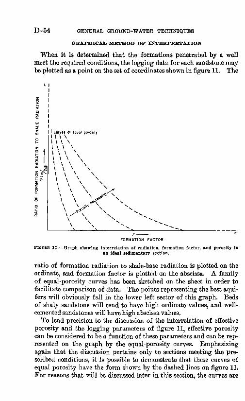
D-54 GENERAL GROUND-WATER TECHNIQUES
GRAPHICAL METHOD OF INTERPRETATION
When it is determined that the formations penetrated by a well meet the required conditions, the logging data for each sandstone may be plotted as a point on the set of coordinates shown in figure 11. The
Curves of equal porosity^ X
' \ \ \
* V \ \ \ X
z
i5*-
<
\ \ \I \ \ \I \ \ \\ \ \ \ \ \ \ \\ \ X N\ \ \ V\ \ \x \» > Afe0. V
\ \ ^° \ X \ v*° N x
\ \ \
\ \F *
FORMATION FACTOR
FIGURE 11. Graph showing interrelation of radiation, formation factor, and porosity in an ideal sedimentary section.
ratio of formation radiation to shale-base radiation is plotted on the ordinate, and formation factor is plotted on the abscissa. A family of equal-porosity curves has been sketched on the sheet in order to facilitate comparison of data. The points representing the best aqui fers will obviously fall in the lower left sector of this graph. Beds of shaly sandstone will tend to have high ordinate values, and well- cemented sandstones will have high abscissa values.
To lend precision to the discussion of the interrelation of effective porosity and the logging parameters of figure 11, effective porosity can be considered to be a function of these parameters and can be rep resented on the graph by the equal-porosity curves. Emphasizing again that the discussion pertains only to sections meeting the pre scribed conditions, it is possible to demonstrate that these curves of equal porosity have the form shown by the dashed lines on figure 11. For reasons that will be discussed later in this section, the curves are
ELECTRICAL AND RADIOACTIVE WELL LOGGING D-55
shown only for the region of sandstone and shaly sandstone; they are not extended into the region of shale.
The condition that no change in porosity occurs along the curves may be expressed by stating that the directional derivative of porosity along the curves is everywhere zero. Because porosity is here con sidered as a function of the two variables, 7 and F, this leads to the condition.
or
-d^ds OT'.OS
where s denotes distance along an equal porosity curve, y is the value of the radioactivity ratio, and F is the formation factor.
O# The derivative >~ is negative, because increases in formation fac
tor at a constant clay content correspond to decreases in porosity. TheO#
derivative ^- is likewise negative, within the region of interest, by
virtue of the assumption that the increase in clay content results in poorer sorting and, therefore, lower porosity. Because these deriva tives have the same sign, the condition of equation 21 can be satisfied
only if j and °^ are opposite in sign, which in turn is true
only if the curves of equal porosity have negative slopes, as shown in figure 11.
The behavior of the equal-porosity curves as the radiation ratio, or clay content, increases, can be discussed on the basis of logging experi ence with shaly formation. Experience has shown that as clay content increases toward the level of a true shale, the change in formation factor produced by a change in porosity decreases rapidly. Because^ 77* 2\A is decreasing, - must increase rapidly as the radiation ratio of
figure 11 increases, and the equal-porosity curves must converge with respect to the variable F. Referring to equation 21, moreover, it can
be seen that because neither nor can be expected to increase07 ds ~*.jfi
rapidly as the clay content increases,- must decrease toward zero inOS
o#order to balance the increase in -. The slope of the equal-porosityor
curves must, therefore, aproach the vertical as the radiation ratio in creases, as indicated in figure 11.
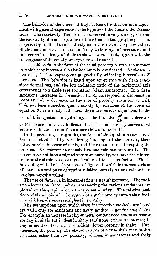
D-56 GENERAL GROUND-WATER TECHNIQUES
The behavior of the curves at high values of radiation is in agree ment with general experience in the logging of the fresh-water forma tions. The resistivity of sandstone is observed to vary widely, whereas the resistivity of shale, regardless of location or stratigraphic position, is generally confined to a relatively narrow range of very low values. Shale must, moreover, include a fairly wide range of porosities, and this general tendency of shale to show low resistivity agrees with the convergence of the equal porosity curves of figure 11.
To establish fully the form of the equal-porosity curves, the manner in which they intercept the abscissa must be considered. As shown in figure 11, the intercepts occur at gradually widening intervals as F increases. This behavior is based upon experience with clean sand stone formations, and the low radiation ratio of the horizontal axis corresponds to a shale-free formation (clean sandstone). In a clean sandstone, increases in formation factor correspond to decreases in porosity and to decreases in the rate of porosity variation as well. This has been described quantitatively by relations of the form of equation 9; as already indicated, there are serious objections to the
50use of this equation in hydrology. The fact that ^-= must decreaseof
as F increases, however, indicates that the equal-porosity curves must intercept the abscissa in the manner shown in figure 11.
In the preceding paragraphs, the form of the equal-porosity curves has been established by considering the slope of these curves, their behavior with increase of shale, and their manner of intercepting the abscissa. No attempt at quantitative analysis has been made. The curves have not been assigned values of porosity, nor have their inter cepts on the abscissa been assigned values of formation factor. This is in keeping with the basic purpose of figure 11, which is the comparison of sands in a section to determine relative porosity values, rather than absolute porosity values.
The use of figure 11 in interpretation is straightforward. The radi ation-formation factor points representing the various sandstones are plotted on the graph or on a transparent overlay. The relative posi tions of these points in the system of equal porosity curves then indi cate which sandstones are highest in porosity.
The assumptions upon which these interpretive methods are based are valid only for sandstone and shaly sandstone, not for true shales. For example, an increase in clay-mineral content need not mean poorer sorting in shale (as it does in shaly sandstone); thus, an increase in clay-mineral content need not indicate lower porosity in shales. Fur thermore, the poor aquifer characteristics of a true shale may be due to causes other than low porosity, whereas in sandstones and shaly
ELECTRICAL AND RADIOACTIVE WELL LOGGING D-57
sandstones porosity normally has an important influence on hydraulic properties. For these reasons, it is considered pointless to extend the equal-porosity lines of figure 11 into the region of true shale.
In employing the method outlined here, the interpreter should al ways first establish whether or not the well penetrates a sequence of beds meeting the necessary requirements. If figure 11 is used to com pare sandstones which do not meet these conditions, the results may be misleading. Where it is uncertain whether or not the geology meets the required conditions, the methods of this section may be used in a reverse sense, in combination with flowmeter work, to provide some information on the nature of the aquifers. If flow measurement shows that the sandstones that plot most favorably on figure 11 are actually the zones of highest yield, the original assumptions are probably satis fied to some extent. For example, porosity and permeability can be considered to be primary, and the best aquifers are the sandstones ex hibiting the highest relative porosities. It may be possible also to assign some reason for the performance of certain of the zones. For example, it may be possible to tell whether a zone has a low yield be cause it is shaly or because it is a relatively "tight" clean sandstone.
The procedures discussed in this section are designed to help the interpreter evaluate aquifers by using radioactivity logs in conjunc tion with other logging data. The restrictions of these methods have been outlined, and it is hoped that those using the methods will do so with these restrictions in mind.
CONCLUSION
Although the several types of logs are, for the most part, discussed separately in this paper; they should never be interpreted separately. A given feature on a log of one type usually can be attributed to any of several possible causes; commonly an examination of the other types of logs for the well will serve to eliminate all except one of these causes. Where possible, logs and flow-tracing experiments should be run as the well is pumped, for comparison with those made under static conditions. Finally, the interpreter should consider all available data from other sources before attempting interpretation. Each in terpretation should be based upon an understanding of logging theory and well hydraulics, rather than upon any memorized set of interpre tive principles.
REFERENCES
Archie, G. B., 1942, The electrical resistivity log as an aid in determining some reservoir characteristics: Am. Inst. Mining Metall. Engineers Trans., v. 146, p. 54-62.
Bell, K. G., 1954, Uranium and thorium in sedimentary rocks, in Nuclear geol ogy a symposium: New York, John Wiley & Sons, p. 98-114.
D-58 GENERAL GROUND-WATER TECHNIQUES
Bennett, G. D., and Patten, E. P., Jr., 1960, Borehole geophysical methods for analyzing specific capacity of multiaquifer wells: U.S. Geol. Survey Water- Supply Paper 1536-A, 25 p.
Brannon, H. B., Jr., and Osaba, J. S., 1956, Spectral gamma-ray logging: Am. Inst. Mining Metall. Engineers Tech. Kept. 4208.
DeWitte, Leendert, 1955, A study of electric log interpretation methods in shaly formations: Am. Inst. Mining Metall. Engineers, Petroleum Trans., v. 204, p. 103-110.
Faul, Henry, 1954, Nuclear logging of drill holes for mineral exploration and soil studies, in Nuclear geology a symposium: New York, John Wiley & Sons, Inc., p. 250-255.
Glasstone, S., 1951, An introduction to electrochemistry: New York, D. Van Nostrand Co.
Grim, R. E., 1953, Clay mineralogy: New York, McGraw-Hill Book Co., 384 p.Guyod, Hubert, 1952, Electrical well logging fundamentals: Houston, Tex.,
164 p.Johnson, D. H., 1954, Radiometric prospecting and assaying, in Nuclear geol
ogy a symposium: New York, John Wiley & Sons, p. 219-241.Jones, P. H., and Skibitzke, H. E., 1956, Subsurface geophysical methods in
ground-water hydrology, in Advances in Geophysics: New York, Academic Press, v. 3, p. 241-300.
Kozary, M. T., 1948, Streaming potentials in electrical well logging: Pennsyl vania State Coll. Bull., v. 43, no. 8, p. 76-96.
Larsen, E. S., Jr., and Phair, George, 1954, Distribution of uranium and thorium in igneous rocks, in Nuclear geology a symposium: New York, John Wiley & Sons, p. 75-89.
McCardell, W. M., and others, 1953, Origin of the electric potential observed in wells: Am. Inst. Mining Metall. Engineers, Petroleum Trans., v. 198, p. 41-50.
Rankama, Kalervo, and Sahama, J. G., 1950, Geochemistry: Chicago, 111., Univ. Chicago Press, 911 p.
Russell, W. L., 1941, Well logging by radioactivity: Am. Assoc. Petroleum Geologists Bull., v. 25, no. 9, p. 1768-1788.
Schlumberger Well Surveying Corp., 1950, Interpretation handbook for resistiv ity logs (Schlumberger Doc. No. 4) : Houston, Tex., Schlumberger Well Sur veying Corp., July 1950.
Senftle, F. E., 1948, The effect of potassium in prospecting for radioactive ores: Canadian Mining Jour. 69, no. 11, p. 55-57.
Theis, C. V., 1938, The significance and nature of the cone of depression in ground water bodies: Economic Geology, v. 33, no. 8, p. 889-902.
Whitehead, W. L., 1954, Hydrocarbons formed by the effects of radioactivity and their role in the origin of petroleum, in Nuclear geology a symposium: New York, John Wiley & Sons, p. 195-218.
Winsauer, W. O., and McCardell, W. M., 1953, Ionic double layer conductivity in reservoir rock: Am. Inst. Mining Metall. Engineers, Petroleum Trans., v. 198, p. 129-134.
Wyllie, M. R. J., 1949, A quantitative analysis of the electrochemical component of the S.P. curve: Am. Inst. Mining Metall. Engineers Trans., v. 186, p. 17-26.
1955, Role of clay in well-log interpretation: California Div. Mines Bull. 169, p. 282-305.
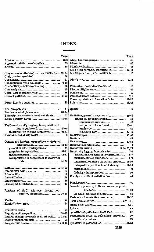
INDEX
Page Apatite... -. .. D49Apparent resistivities of aquifers ... 13 Arkose_ ..__ 49
Clay minerals, effects of, on rock resistivity... 10, 24Coal, uranium-enriched..._ . 50Conclusion . 57Conduction in earth materials.___.-_... 9-10Conductivity, factors controlling.. .. ... 40Core analysis____._.__.. _ 19Curie, unit of radioactivity__ . 46Current patterns.__ ___-----_ 3,22
Direct-junction equation.
Effective porosity.... __ 54 Electrochemical phenomena. .. 33-34 Electrolytic characteristics of well fluids. 11 Equal-porosity curves....__.. ... 55-56
Fluid-conductivity logging, interpretation, inmultiaquiferwell. ____-___- 41-45
interpretation in single-aquifer well__ 40-41Formation-resistivity factor.... _ 9
Gamma-ray logging, assumptions underlyinginterpretation..___.. .._ 52-53
general lithologic interpretation 61 graphical interpretation.... ___ 54-57 instrumentation_____________. 45-47 interpretation as supplement to resistivity
data... .. . 51-62
Illite___....__.._...... . .. 48,49Interaquifer flow 37 Introduction . 1-2 Ionic diffusion.____ ........ .... .. 28Ionic transport___________.__ 16 Isomorphic substitution.._ 49
Junction of NaCl solutions through ion- selective membrane___. ___ 30-31
EaoUn............ - - 48Kirchoff'sloop rule. . .. 34
Limestone sonde..... .... .. 23Liquid-junction equation__........___.. 29-30Liquid-junction potentials in an oil well. 32-34 Liquid-junction problem. 28 Long-normal device. _~ 2,7,8,11
Page Mica, hydrous groups.._------_------ D48Monazite____________________ 49 Montmorillonite________________ 48 Mud-filled borehole, conditions in____... 13-14 Multiaquifer well, internal flow in_ ____ 15
Ohm's law... ________________.. 5,36
Permeable zones, identification of____ . 12 Photomultiplier tube_____________ 46 Plagioclase______.____._____.. 49 Point-resistance device.__________... 7,8 Porosity, relation to formation factor. ____ 18-20 Potassium______.____________ 46,48
Quartz. 49
Radiation, general discussion of._ __ .. 45-46sources of, carbonate rocks.. _______ 50
common sediments__________ 47evaporite rocks and coal._______ 50-51sandstone...._____________ 49shale and clay__ _____... 47-49
Radioisotopes.. ___.._._.___._.. 45-46 Kadium.-. .. _ 49 References___________________ 57-58 Resistance, formula for. ___________ 4 Resistivity curves..... . ....... 17,24,25,26Resistivity logging, borehole effect______ 7-9
calibration and zones of investigation.. _ 6-7 instrumentation and theory..___..... 2-9interpretation based on normal curves.... 11-19interpretive practices in oil industry.._ 11-13introduction_._.___._..___.. 2lithologic interpretation--. ________ 10
Roentgens, units of radiation flux_... _. _ 46
Scintillometer..._._._..............__ 46Secondary porosity, in limestone and crystal
line rocks.____.____.__ 20-24in sandstone-shale sections________ 24
Shale as an ion-selective membrane.. .. . 31-32 Short-normal device___ _.. 2,7,8,11 Single-point device.___________. 6,11 Sphene__________________..... 49 Spontaneous-potential current loop. 34 Spontaneous-potential deflections, abnormal. 39
artificially induced- ____._.._.... 39 Spontaneous-potential log.... .... 31,33
D59
D60 INDEX
Page Spontaneous-potential logging, analysis of
quantitative interpretation. _ D-27-29 history.___________________ 27 Instrumentation____________.. 26-27 objections to quantitative interpretation
for water wells_.________ 36-37 recognizing mineralized-water zones..._ 38 summary. . ...__.________ 39
Spontaneous-potential measurement relatedto emf... _______.___ 34-36
Storage coefficient___ _________ 51
Page Streaming potentials.... ....__.____ D-38
Thorium___._....._....-_____.__ 46,49 Tourmaline____________________ 48,49 Transmissibility coefficient___ ______ 51
Uranium. 46
Water-filled borehole, conditions in. 14-17 Well fluids, electrolytic characteristics__. _ 11
Zircon__________ __.._ __ 48,49
U. S. GOVERNMENT PRINTING OFFICE : 1967 O - 249-459