i

APPLICATION OF ECONOMIC ORDER QUANTITY WITH QUANTITY

DISCOUNT MODEL. A CASE STUDY OF WEST AFRICAN

EXAMINATION COUNCIL

BY

EMMANUEL ADJIN OKWABI (BEd. MATHEMATICS)

PG 6323111

A Thesis Submitted to the Department of Mathematics, Kwame Nkrumah University of

Science and Technology, Kumasi, in Partial fulfillment of the requirement for the

degree of

MASTER OF SCIENCE: Industrial Mathematics,

College of Science / Institute of Distance Learning

JANUARY, 2014

ii

DECLARATION

I hereby declare that this submission is my own work towards the MSc. Degree and that,

to the best of my knowledge; it contains neither material previously published by another

person nor material, which has been accepted for the award of any other degree of the

University, except where the acknowledgement has been made in the text.

Emmanuel Adjin Okwabi (20250483) ..……………. ………………

Student’s Name & ID No. Signature Date

Certified by:

Prof. S.K Amponsah ……………….. ………………

Supervisor’s Name Signature Date

Certified by:

Prof. S. K Amponsah ……………… ……………... Head of Dept. Name Signature Date

Certified by:

Prof. I. K Dontwi ……………… ........................ Dean-IDL Signature Date

iii

DEDICATION

This Thesis is dedicated to the Almighty Jehovah through whose Sufficient Grace and

infinite Mercies and Love I have come this far; and to my family members and friends

especially Mr. Maxwell Ofosu who supported me by way of finance, directions and

encouragement. Finally, to all my lecturers especially those in the Mathematics

Department of the Institute of Distance Learning, Kwame Nkrumah University of

Science and Technology.

iv

ACKNOWLEDGEMENT

My first and foremost profound gratitude goes to Jehovah, the ever living Father, whose

sustenance, guidance and protection has made this Thesis a success.

My heartfelt gratitude goes to my ever devoted and dedicated supervisor and Lecturer,

Prof. S. K. Amponsah whose direction, encouragement, corrections, discussions and

suggestions have made this piece of work a reality.

Again my appreciation goes to my lovely parents for their relentless effort to see me

through my education. I also thank all the lecturers of the Industrial Mathematics

Programme in the Institute of Distance Learning of the KNUST.

And to my friends Maxwell Ofosu, Seth Asiedu, Albert Cudjo, Rose Vossah, Sandra

Tenkorang and all others I cannot remember who supported me in diverse ways, I say, I

am very grateful.

May the Almighty God bless each and every soul beyond measure who in diverse ways

has contributed to this work.

v

ABSTRACT

The Economic Order Quantity (EOQ) is a pure economic model in the classical inventory

control theory. The model is designed to find the order quantity so as to minimize the

total average cost of replenishment under deterministic demand and some simplifying

assumptions. The study focuses on inventory management when the unit purchasing cost

decreases with the order quantity, Q. The main objective of the study is to model

Economic Order Quantity with quantity discount to achieve optimal level of inventory.

The model was analyzed against the current practices of the West African Examination

Council, (WAEC) ordering policies to find out whether it is appropriate to go for quantity

discount when offered. The Management of WAEC wants to determine if it should take

advantage of the discount or order basic EOQ order size offered to them by their

suppliers. The 2012 data was used for the analysis, (as shown in table 4.1, page 65). From

the analysis it was observed that a discount price of GHȼ890 000.00 is the minimum

price that gives the minimum quantity of 350 000. There is no order size larger than 350

000 that would results in a lower price. This means that the company should spend a total

cost of eight hundred and ninety thousand Ghana cedis, (GHȼ890 000.00) to order an

optimal quantity of three hundred and thirty thousand, (350 000) units of materials.

The management will benefit from the proposed approach for their inventory control

management system; this could help them take informed decision. The study

recommends that the model should be adopted by the company for their inventory control

and management planning.

vi

CONTENT

DECLARATION ................................................................................................................. i

DEDICATION .................................................................................................................... ii

ACKNOWLEDGEMENT ................................................................................................. iv

ABSTRACT ........................................................................................................................ v

1.0 INTRODUCTION ........................................................................................................ 1

1.1BACKGROUND OF STUDY ....................................................................................... 2

1.2 PROBLEM STATEMENT ........................................................................................... 9

1.3 OBJECTIVES ............................................................................................................. 10

1.4 METHODOLOGY ..................................................................................................... 10

1.5 JUSTIFICATION ....................................................................................................... 11

1.6 SIGNIFICANCE OF THE STUDY............................................................................ 11

1.7 LIMITATION OF THE STUDY ................................................................................ 11

1.8 ORGANIZATION OF THE STUDY ......................................................................... 12

1.9 SUMMARY ................................................................................................................ 12

2.0 INTRODUCTION ...................................................................................................... 14

2.1 THEORITICAL LITERATURE ................................................................................ 14

2.2 CLASSICAL INVENTORY MODEL ....................................................................... 18

2.3 EMPIRICAL LITERATURE ..................................................................................... 20

2.3.1 EOQ BASED ON UNCERTAIN THEORY ....................................................... 23

vii

2.4 APPROACHES TO DEAL WITH RANDOMNESS AND FIZZINESS .................. 24

2.4.1 FUZZY ECONOMIC ORDER MODEL............................................................. 25

2.4.2 RANDOM ECONOMIC MODEL ...................................................................... 26

2.6 EOQ CONSIDERING TRADE-OFF ......................................................................... 31

2.7 PERIODIC-REVIEW INVENTORY MODEL .......................................................... 35

2.8 EOQ UNDER CONDITIONALLY PERMISSIBLE DELAY................................... 37

2.9 ORDER QUANTITY REORDER POINT MODEL .................................................. 44

2.10 EOQ WITH QUANTITY DISCOUNT .................................................................... 44

2.11 SUMMARY .............................................................................................................. 48

3.0 INTRODUCTION ...................................................................................................... 49

3.1 DEFINITION OF VARIABLES ................................................................................ 50

3.2 THE BASIC EOQ MODEL........................................................................................ 50

3.3 THE EOQ MODEL WITH QUANTITY DISCOUNTS ............................................ 54

3.3.1 All Units Discount ............................................................................................... 56

3.3.2 An Algorithm to Determine the Optimal Order Quantity for the All .................. 58

3.3.3 Incremental Quantity Discount ............................................................................ 59

3.4 An Algorithm to Determine the Optimal Order Quantity for the ........................... 62

3.4 SUMMARY ................................................................................................................ 62

4.0 INTRODUCTION ...................................................................................................... 63

4.1 DATA COLLECTION AND ANALYSIS ................................................................. 63

viii

4.2 RESULTS ................................................................................................................... 66

4.3 CONCLUSIONS......................................................................................................... 67

5.0 INTRODUCTION ...................................................................................................... 69

5.1 CONCLUSIONS......................................................................................................... 69

5.2 RECOMMENDATIONS ............................................................................................ 70

REFERENCES: ................................................................................................................ 71

1

CHAPTER ONE

1.0 INTRODUCTION

In recent years, Inventory Management (IM) has attracted a great deal of attention from

people both in academia and industries. A lot of resources have been devoted into

research in the inventory management practices of organizations. Companies with

superior forecasting abilities can afford to procure or produce large fractions of their

demand by making use of low production methods and inexpensive logistics services.

These companies pay more for faster production and logistics services only when the

demand surges or goes up unexpectedly. On the other hand, companies with irregular

demands and inferior forecasting abilities have to pay more for using fast production

methods to respond to unexpected surges in demand.

The advances in manufacturing technologies, logistics services, and globalization makes

it possible for companies to satisfy their customer demands from sources with different

prices and lead time. On the other hand the ability to provide better forecasting increases

as the delivery date approaches and the cost increases as the lead time increases.

It is critical to be able to simulate in advance the demand information, lead time in

logistics services and to strike a balance between the quality of demand information and

the cost of production and logistics services.

With today’s uncertain economy, companies are searching for alternative methods to

keep ahead of their competitors by effectively driving sales and by cost reduction. Big

retail companies do not stand a chance in today’s environment if they do not have an

appropriate inventory control model intact. The Economic Order Quantity and a Reorder

2

Point (EOQ/ROP) model have been used for many years, but yet some companies have

not taken advantage of it. An Economic Order Quantity could assist in deciding what

would be the best optimal order quantity at the company’s lowest price. Similar to EOQ,

the reorder point will advise when to place an order for specific products based on their

historical demand. The reorder point also allows sufficient stock at hand to satisfy

demand while the next order arrives due to the lead time.

The Economic Order Quantity model is a pure economic model in the classical inventory

control theory. The model is designed to find the order quantity so as to minimize the

total average cost of replenishment under deterministic demand and some simplifying

assumptions. These assumptions are unrealistic; however, simplicity and robustness of

the model makes it practical in most cases.

1.1BACKGROUND OF STUDY

Economic order quantity (EOQ) model is one of fixed order quantity models of inventory

problem. In EOQ, we need to determine the optimal selling period and order quantity.

EOQ is also known as that shortage which is not permitted and production time being

very short affect the inventory model. The EOQ model was proposed by Harris in 1913

and subsequently by Wilson in 1934, it was the initial lot size model based on cost

minimization. Many extensions of the Harris’ EOQ model have been constructed and

solved through the formulation of different assumptions. Among others are the cases

when shortage is permitted. A group of these models assumes that, in the case of a

shortage, the customer is waiting for the delivery of the next order, at which time is

demand will be fulfilled. In the classical inventory models, the issue of quality is ignored.

In other words, it implicitly assumes that the quality level is fixed at an optimal level and

3

not subject to control. However, in a real production environment, it can be observed that

there are defective items being produced. These defective items must be rejected,

repaired, reworked, or, if they have reached the customer, refunded, and hence, extra

costs are incurred. Therefore, it is important to take the quality-related cost into account

in determining the optimal ordering policy (Lixia, 2011).

The Economic Order Quantity is the number of units that a company should add to

inventory with each order to minimize the total costs of inventory such as holding costs,

order costs, and shortage costs. The EOQ is used as part of a continuous review inventory

system, in which the level of inventory is monitored at all times, and a fixed quantity is

ordered each time the inventory level reaches a specific reorder point. The EOQ provides

a model for calculating the appropriate reorder point and the optimal reorder quantity to

ensure the instantaneous replenishment of inventory with no shortages. It can be a

valuable tool for small business owners who need to make decisions about how much

inventory to keep on hand, how many items to order each time, and how often to reorder

to incur the lowest possible costs (Muhammad and Omar, 2011).

The EOQ model assumes that demand is constant, and that inventory is depleted at a

fixed rate until it reaches zero. At that point, a specific number of items arrive to return

the inventory to its beginning level. Since the model assumes instantaneous

replenishment, there are no inventory shortages or associated costs. Therefore, the cost of

inventory under the EOQ model involves a trade-off between inventory holding costs (the

cost of storage, as well as the cost of tying up capital in inventory rather than investing it

or using it for other purposes) and order costs (any fees associated with placing orders,

such as delivery charges). Ordering a large amount at one time will increase a small

4

business's holding costs, while making more frequent orders of fewer items will reduce

holding costs but increase order costs. The EOQ model finds the quantity that minimizes

the sum of these costs (Bhavin et al., 2007).

The purpose of the EOQ model is simple, to find that particular quantity to order which

minimizes the total variable costs of inventory. Total variable costs are usually computed

on an annual basis and include two components, the costs of ordering and holding

inventory. Annual ordering cost is the number of orders placed times the marginal or

incremental cost incurred per order. This incremental cost includes several

components: the costs of preparing the purchase order, paying the vendor's invoice, and

inspecting and handling the material when it arrives. It is difficult to estimate these

components precisely but a ball-park figure is good enough. The EOQ is not especially

sensitive to errors in inputs (www.usersolutions.com).

The holding costs used in the EOQ should also be marginal in nature. Holding costs

include insurance, taxes, and storage charges, such as depreciation or the cost of leasing a

warehouse. One should also include the interest cost of the money tied up in inventory.

Many companies also add a factor to the holding cost for the risk that inventory will spoil

or become obsolete before it can be used (www.usersolutions.com).

Inventories are essential for keeping the production wheels moving, keep the market

going and the distribution system intact. They serve as lubrication and spring for the

production and distribution systems of organizations. Inventories make possible the

smooth and efficient operation of manufacturing organizations by decoupling individual

segments of the total operation. Purchased parts inventory permits activities of the

purchasing and supply department personnel to be planned, controlled and concluded

5

somewhat independently of shop-product operations. These inventories allow additional

flexibility for suppliers in planning, producing and delivering an order for a given

product’s part, Lonergan (2003) Inventory is essential to organization for production

activities, maintenance of plant and machinery as well as other operational requirements.

This results in tying up of money or capital which could have been used more

productively. The management of an organization becomes very concerned in inventory

stocks are high. Inventory is part of the company assets and is always reflected in the

company’s balance sheet. This therefore calls for its close scrutiny by management,

Sallemi (1997) Management is very critical about any shortage of inventory items

required for production. Any increase in the redundancy of machinery or operations due

to shortages of inventory may lead to production loss and its associated costs. These two

aspects call for continuous inventory control. Inventory control and management not only

looks at the physical balance of materials but also at aspects of minimizing the inventory

cost. The classic dilemma in inventory management is maintained in high service levels

to meet the needs of customers while avoiding high stocks regardless of the type of items

or even the department for which such stock is purchased.

To be successful, most businesses other than service businesses are required to carry

inventory. In these businesses, good management of inventory is essential.

The management of inventory requires a number of decisions. Poor decision making

regarding inventory can cause:

(i) Loss of sales because of stock outs.

(ii) Depending on circumstances, inadequate production for a period of time.

6

(iii) Increases in operating expenses due to unnecessary carrying costs or loss from

discarding obsolete inventory.

(iv) An increase in per unit cost of finished goods.

Of all the activities in a manufacturing business, inventory creation is the most dynamic

and certainly the most visible activity. In one sense, inventory involves all production

activity from the purchase of raw materials to the delivery of finished goods inventory to

the customer. The financial accounting for inventory is concerned primarily with

determining the correct count and the assignment of historical cost. However, from a

management accounting viewpoint, the central focus is on manufacturing the right

amounts at the lowest cost consistent with a quality product. From a financial viewpoint,

poor management of inventory can adversely affect cash flow. Also, excessive inventory

can cause a decrease in return on investment. An over stock of inventory causes total

assets to be larger and certain expenses to increase. Consequently, in addition to a

reduced cash flow, the effect of poor inventory management can be a lower rate of return.

Finished goods inventory represents the company’s product for available for sale at a

given point in time. A certain amount of inventory must be available at all times in order

to have an effective marketing operation. The poor management of inventory, including

finished goods, is often reflected in the use of terms such as such as stock outs, back

orders, decrease in inventory turnover, lost sales, and inadequate safety stock.

The existence of inventory results in expenses other than the cost of inventory itself

which typically is categorized as:

(i) Carrying costs

(ii) Purchasing costs.

7

Inventory is a term that may mean finished goods, materials, and work in process.

In a manufacturing business, there is a logical connection between these three types of

inventory:

Table 1.1: Table showing the logical connection between inventories

Materials

Labour

Overhead

Work in Process

Finished

goods

Cost of goods

sold

To have finished goods inventory, production must take place at a rate greater than sales.

Inventory decisions have a direct impact on production. For example, a decision to

increase safety stock means that the production rate must increase until the desired level

of safety stock is achieved.

From an accounting standpoint, there are two main areas of concern. First, from a

financial accounting viewpoint, the main accounting problems concern:

(i) The flow of costs (FIFO, LIFO, average cost)

(ii) Use of a type of inventory costing method (periodic or perpetual)

(iii) Taking of physical inventories.

(iv) Techniques for estimating inventory

From a financial accounting viewpoint, the cost assigned to inventory directly affects net

income. If ending inventory is overstated, then net income is overstated and conversely, if

ending inventory is understated then net income is understated.

Also, the use of direct costing rather than absorption costing can affect net income. From

a management accounting viewpoint, there are variety of inventory decisions that affect

8

net income. Decisions regarding inventory can be placed in two general categories: (1)

those decisions that affect the quantity of inventory and (2) those decisions that affect per

unit cost of inventory.

Decisions that affect the quantity of inventory

(i) Order size

(ii) Number of orders

(iii) Safety stock

(iv) Lead time

(v) Planned production

Decisions that affect the cost per unit of inventory

(i) Suppliers of raw material (list price and discounts)

(ii) Order size (quantity discounts)

(iii) Freight

In addition, decisions pertaining to labour and overhead also indirectly affect per unit cost

of inventory. In a manufacturing business, the costs of labour and overhead do not

become operating expenses until the manufacturing costs appear as part of cost of goods

sold. Labour and overhead costs are deferred in inventory until the inventory has been

sold.

The main management accounting tool that may be used to make inventory purchase

decisions is the EOQ model. This tool recognizes that there are two major decisions

regarding the materials inventory: (i) orders size and (ii) number of orders.

There are consequently two major questions:

(i) How many units should be purchased each time a purchase is made (order size)?

9

(ii) How many purchases should be made (number of orders)?

To understand an EOQ model, it is essential that the concept of average inventory be

understood. Inventory is never static and is constantly rising and falling over time, even

in the very short term. Inventory, for example, rises when raw materials are purchased

and falls when raw material is used. Because inventory in a business is constantly

changing, it is necessary to think in terms of average inventory levels.

The high points and low points of inventory are easy to explain and illustrate, if a

purchasing policy is consistently applied and the rate of usage of raw material is uniform.

Inventory is at its highest and lowest levels when a new shipment of material arrives.

Theoretically, in absence of a need for safety stock, a new shipment should arrive at the

moment inventory reaches zero. Immediately, upon arrival of a new shipment, inventory

is then at its highest level again.

1.2 PROBLEM STATEMENT

The most common problem in inventory management is to attain optimal inventory

levels. Decisions about how many of which products are to be stored in the warehouse,

when to place the next order, the quantities to be ordered are some of the problems

encountered every day. High level of inventory locks up the capital of any company.

Customers on the other hand, lose confidence in the company and look elsewhere if there

is no availability. This can reduce the profitability of the company and eventually

crumple the company.

Our study focuses on inventory management when the unit purchasing cost decreases

with the order quantity Q. In other words, a discount is given by the seller if the buyer

purchases a large number of units. Our objective is to determine the optimal ordering

10

policy for the buyer in the presence of such incentives. We will discuss two types of

quantity discount contracts: all units’ discounts and incremental quantity discounts.

1.3 OBJECTIVES

The objectives of the study are to:

(i) Economic Order Quantity with quantity discount will be modelled to achieve

optimal level of inventory. This implies cost saving in inventory control and

achievement of maximum profit. Carrying cost would be reduced to the

lowest possible value so that the extra money can be invested in other parts of

the company.

(ii) This Economic Order Quantity Model will be analysed against the current

practices of WAEC ordering policies. The goal is to enable the company to

analyse whether it is appropriate to go for quantity discount when offered or

not.

(iii) Finally, the best policy in Managing Inventory will be determined through the

Economic Order Quantity with discount model procedures and methods.

1.4 METHODOLOGY

Optimization procedures of the Economic Order Quantity is an effective tool to model,

analyze and optimize any inventory systems. It is useful in forecasting the behaviour of

systems with both continuous and discrete variables like a typical inventory system.

Discrete and continuous systems need to be modeled or designed into complex systems.

11

This complex system or model must be linked with a specific simulation optimization

technique that best calculate the output.

In our methodology, we shall apply the economic order quantity with discount model

optimization procedures and methods in solving our problem.

1.5 JUSTIFICATION

Many companies blindly purchase in large quantities to get discount prices without

considering all the tradeoffs involved. The costs may well outweigh any savings in

purchase price. The economic order quantity with discount model helps to analyze

quantity discount offers and make better purchasing decisions, hence the reason for the

study.

1.6 SIGNIFICANCE OF THE STUDY

The findings of the study will provide well–researched information, which can be useful

to researchers for academic purposes in the area of inventory management. To the stores

and Procurement department staff, the study hopes to provide them with useful

information like the recommended techniques of inventory control so as to meet their

customer’s and organization’s needs. To the firm’s management, the recommendations of

the study may enable them to design inventory management policies to improve the

smooth running of the firm, thereby satisfying customers and generally minimizing costs.

1.7 LIMITATION OF THE STUDY

The study is limited to economic order quantity model with quantity discount on volume

of goods purchased, thus other types of economic order quantity model such as those

12

with price peak and shortages will not be covered in this study. This is a deliberate effort

on the researcher’s part to make the study manageable given the time and resources

available to the researcher to complete the study. The study was limited to the perceived

effect of economic order quantity model with quantity discount on volume of goods

purchased on management decision making on the inventory control of the West African

Examinations Council.

1.8 ORGANIZATION OF THE STUDY

In chapter one, we presented a background study of economic order quantity model.

In chapter two, related work in the economic order quantity model would be discussed.

In chapter three, the economic order quantity with discount model optimization

procedures and methods that would be applied in solving our problem will be introduced

and explained.

Chapter four will provide a computational study of the algorithm applied to our economic

order quantity with discount instances.

Chapter five will conclude this thesis with additional comments and recommendations

1.9 SUMMARY

The inventory system has diverse decision variables that can be considered as continuous

like regular orders, demand on the stock, regular supply et cetera. On the other hand,

there are discrete variables like special orders that come in at a particular time, theft or

accidents that occur without any warning. Based on the kind of information that

management or decision makers need to enable them plan properly for their inventory,

13

these discrete and continuous variables always play an important role in determining the

results.

This study seeks to solve an economic order quantity problem with quantity discount and

proposed the economic order quantity with discount model optimization procedures and

methods in solving the problem.

In the next chapter, we shall put forward pertinent literature on Economic Order Quantity

Models. And also review both theoretical and empirical works of EOQ under different

conditions of inventory management.

14

CHAPTER TWO

LITERATURE REVIEW

2.0 INTRODUCTION

This chapter of the study reviews both theoretical and empirical works of EOQ under

different conditions. This chapter will also review literature on other different types of

inventory management.

2.1 THEORITICAL LITERATURE

The Economic Order Quantity (EOQ) model is a pure economic model in classical

inventory control theory. The model is designed to find the order quantity so as to

minimize total cost under a deterministic setting. Arslan and Metin (2010) revised the

standard EOQ model to incorporate sustainability considerations to include

environmental and social criteria in addition to the conventional economics. The authors

proposed models for a number of different settings and analyze these revised models.

Based on their analysis, they showed how these additional criteria can be appended to

traditional cost accounting in order to address sustainability in supply chain management.

The authors proposed a number of useful and practical insights for managers and policy

makers.

Hoen et al., (2010) developed models for transport mode selection problem with emission

costs and constraints. Their model is based on the classical newsboy model. The authors

argued that emission cost accounting, emission tax or emission trade mechanisms all fail

if the aim is to curb the emissions. On the other hand, a direct cap on emissions works.

15

They also calculated emissions for different transport mode choices to estimate the

parameters of the proposed models.

Hua et al., (2009) investigated the effect of carbon emissions in inventory control. The

authors extended the standard EOQ model to further account for the carbon emissions

under cap and trade mechanism. The authors proposed a number of insights based on

their analytical and numerical analysis and provided conditions of buying and selling

carbon credit while reducing costs, emissions and in some cases, both of them.

An inventory management system for defective items with backordered shortages is

explored, in which we assume that the quality of an ordered lot is not always 100%

perfect, so a screening process to each product is conducted to split that lot into perfect

and defective products. Meanwhile, the defective products include imperfect and scrap

ones, which will be sold at a discount price and disposed of at a cost, respectively. Kuo-

Hsien et al., (2008) presented a model for finding the optimal order size and optimal

backorder level for each cycle by minimizing a simpler objective of expected total cost

per unit time, instead of utilizing the somewhat complex expected total profit per unit

time in Eroglu and Ozdemir’s (2007) model. Sequentially, the authors also made

numerous previous models as special cases of their model.

Most existing economic order quantity models appearing in the literature have been

developed by assuming that an ordered lot received at the beginning of a selling period is

100% perfect in quality. However, it may not be pertinent to real market environments,

not only because of production processes, but also because of delivery processes or other

16

unexpected factors, all of which might more or less damage the products’ quality. Porteus

(1986) presented an EOQ model in association with the effect of detective items, where a

probability that a production process would go out of control is hypothesized.

Rosenblatt and Lee (1986) assumed that timing from the beginning of a production run to

an uncontrollable process is an exponential distribution and the defective products can be

reworked at that instant moment with an extra cost.

Salameh and Jaber (2000) extended the traditional EOQ problem by accounting for

imperfect products in which an ordered lot is 100% screened, and that resulting imperfect

products will be sold at a single batch when the screening process is completed. Later an

error in their result toward the optimal order size was corrected by Cardenas-Barron

(2000), showing that the denominator of the expression regarding the optimal order size

should be multiplied by a factor of “2”.

Papachristos and Konstantaras (2006) investigated the model with a proportional

imperfect quality, which is a random variable. They expanded the models to the case that

the defectives are withdrawn at the end of planning horizon, other than at the end of the

screening process.

Eroglu and Ozdemir (2007) developed a related model with stock-out occurrence, during

which shortages are backordered and the defective products, containing imperfect and

scrap ones, will be sold at cheaper price and / or discarded at cost.

There have been many inventory models with partial backordering, but few of them

considered the case where the unmet demand can be satisfied by the substitutable item.

Renqian et al., (2010) presented a two-item deterministic EOQ model, where the demand of

17

one item can be partially backordered and part of its lost sales can be satisfied for by the

substitution. The authors’ analysis provided a tractable and accurate method to determine

order quantities and order cycles for the two items. The optimal solutions of the model, as

well as the inventory decision procedures, were also developed.

Generally, if stock outs happen, the unmet demand can be either backordered or lost. If

the unsatisfied customers are willing to wait, then their demand can be met in the next

replenishment epoch. Otherwise, they may buy their desired items from other suppliers,

and the unmet demand is therefore lost immediately. In practice, the most frequent case is

that some of the unsatisfied customers may be willing to wait and backorder their unmet

demands while some others may purchase their desired items from another vendor, which

represents the case of partial backordering. Montgomery et al. (1973) presented the first

model on EOQ with partial backordering, assuming that a fixed fraction of demand

during the stock-out period is backordered, and the remaining fraction is lost.

After that, Rosenberg (1979), Park (1982), and Pentico and Drake (2009a) proposed

some similar EOQ models with partial backordering. If there are some similar items in

stock, substitutions may occur when one of the demanded items is stocked out.

During all the stocked out period, the unsatisfied customers may choose another similar

item, which forms an inventory problem of the EOQ with substitution. The earliest

literature refers to the substitution of products is Veinott (1969).

18

McGillivray and Silver (1978) presented the concepts of substitutable items in inventory

management. They assumed that a proportion of the unmet demand can be satisfied by

another similar item. After that, many studies on inventory models with substitution were

proposed (Parlar and Goyal, 1984; Parlar, 1985; Drezner et al., 1995; Ernst and Kouvelis,

1999; Rajaram and Tang, 2001; Netessine and Rudi, 2003; Nagarajan and Rajagopalan,

2008; Huang et al, 2010).

2.2 CLASSICAL INVENTORY MODEL

In the classical inventory models, the issue of quality is ignored. However, in a real

production environment, it can be observed that there are defective items being produced.

These defective items must be rejected, repaired, reworked, or, if they have reached the

customer, refunded, and hence, extra costs are incurred. Recently some of researchers

explicitly elaborate on the significant relationship between quality imperfection and lot

size. In the recent models although quality entered into the models but none of them have

considered shortage problem. Jafar and Rafsanjan (2005) presented a model for the

extension of the traditional EPQ/EOQ model by accounting for imperfect quality items

when using the backorder EPQ/EOQ formulae. Finally, numerical example is provided to

illustrate the solution procedure and concluding remarks are given.

Porteus (1986) is one of the first researchers who incorporated the effect of defective

items into the basic EOQ model. The author described a system that begins each

production run in control (i.e. producing only good units). As each unit is produced, there

is a probability p that the system goes out of control, at which time all subsequent units

(until the end of the production run) are defective. The time until the process goes out of

19

control therefore follows a geometric distribution. The author used this model to study

the optimal setup investment in relation to reducing the probability p of the process going

out of control. The author’s work has encouraged many researchers to deal with modeling

the quality improvement problems.

Rosenblatt and Lee (1986) presented a model that assumed that the time between the

beginnings of the production run; i.e., the in-control state; until the process goes out of

control is exponential and that defective items can be reworked instantaneously at a cost.

The authors concluded that the presence of defective products motivates smaller lot sizes.

In a subsequent model, Rosenblatt and Lee (1987) considered using process inspection

during the production run so that the shift to out-of-control state can be detected and

restoration made earlier.

A joint lot sizing and inspection policy is studied under an economic order quantity

model where a random proportion of units are defective. Those units can be discovered

only through expensive inspections. Thus, the problem is bivariate. Both lot size and

fraction to inspect are to be chosen. A model is analyzed in which the only penalty for

uninspected defectives is financial. Zhang and Gerchak (1990) considered a joint lot

sizing and inspection policy studied under an EOQ model where a random proportion of

units are defective. The authors considered a model where the defective units cannot be

used and thus must be replaced by non-defective ones. The authors found that a

considerable deviation from the optimal quantity will generally result in only a small

increase in objective function value.

20

Urban (1992) presented a finite replenishment inventory model in which the demand of

an item is a deterministic function of price and advertising expenditures. The formulated

models also incorporate learning effects and the possibility of defective items in the

production process. The author developed a general solution methodology to determine

the optimal lot size, price mark-up, and advertising expenditure simultaneously.

2.3 EMPIRICAL LITERATURE

Chan et al., (2003) provided a framework to integrate lower pricing, rework and reject

situations into a single economic production quantity (EPQ) model. A 100% inspection is

performed in order to identify the amount of good quality items, imperfect quality items

and defective items in each lot. The authors assumed that items of imperfect quality, not

necessarily defective, could be used in another production situation or sold to a particular

purchaser at a lower price.

Ouyang and Chang (2000) investigated the impact of quality improvement on the

modified lot size reorder point models involving variable lead time and partial

backorders. The formulated models include the imperfect production process and an

investing option of improving the process quality. The objective is simultaneously

optimizing the lot size, reorder point, process quality level and lead time.

Makis and Fung (1998) studied the effect of machine failures on the optimal lot size and

on the optimal number of inspections in a production cycle. The authors obtained the

formula for the long-run expected average cost per unit time for a generally distributed

21

time to failure and found an optimal production/inspection policy by minimizing the

expected average cost.

Ben-Daya (1999) presented multi-stage lot sizing models for imperfect production

processes. The effect of imperfect quality on lot sizing decisions and effect of inspection

errors are taken into consideration in the proposed models.

Ouyang et al., (2002) investigated the lot size, reorder point inventory model involving

variable lead time with partial backorders, where the production process is imperfect. In

the authors model the options of investing in process quality improvement and setup cost

reduction were included, and lead time can be shortened at an extra crashing cost. The

objective of that model is to simultaneously optimize the lot size, the reorder point, the

process quality, the setup cost, and the lead time.

Chiu (2003) considered the effects of the reworking of defective items on the economic

production quantity (EPQ) model with backlogging allowed. In the authors study, a

random defective rate is considered, and when regular production ends, the reworking of

defective items starts immediately. Not all of the defective items are reworked, a portion

of them are scrap and are discarded. The author derived optimal lot size that minimizes

the overall costs for the imperfect quality EPQ model where backorders are permitted.

Goyal et al., (2003) developed a simple approach for determining an optimal integrated

vendor-buyer inventory policy for an item with imperfect quality.

22

Ouyang et al., (2003) investigated the integrated vendor-buyer inventory problem, they

assume that an arrival order lot may contain some defective items, and the defective rate

is a random variable. Also, shortage is allowed and the lead time is controllable and

reducible by adding extra crashing cost. The authors derived an integrated mixture

inventory model with backorders and lost sales, in which the order quantity, reorder

point, lead time and the number of shipment from vendor to buyer are decision variables.

The authors first assumed that the lead time demand follows a normal distribution, and

then relax the assumption about the form of the distribution function of the lead time

demand and applied the minimax distribution-free procedure to solve the problem.

Salameh and Jaber (2000) developed a model to determine the total profit per unit of time

and the economic lot size for a product purchased from a supplier. Each lot of the product

delivered by the supplier contains defective items with a known probability density

function. The purchaser performs a 100% screening process immediately on receiving a

lot. Items of poor quality detected in the screening process of a lot are old at a discounted

price at the end of the screening process of a lot.

Birbil et al., (2009) considered an economic order quantity type model with unit out-of-

pocket holding costs, unit opportunity costs of holding, fixed ordering costs and general

transportation costs. For these models, the authors analyzed the associated optimization

problem and derive an easy procedure for determining a bounded interval containing the

optimal cycle length. Also for a special class of transportation functions, like the carload

discount schedule, the authors specialized these results and give fast and easy algorithms

to calculate the optimal lot size and the corresponding optimal order-up-to-level.

23

2.3.1 EOQ BASED ON UNCERTAIN THEORY

Lixia (2011) presented two new models for Economic Order Quantity (EOQ) for

inventory based on uncertain theory. In the models, the holding cost, shortage cost and

ordering cost per unit are assumed to be uncertain variables. Taking advantages of some

properties of uncertainty theory, the models can be transformed into deterministic form

and solved by 99-method. In the end, two numerical examples are provided to illustrate

the effectiveness of the models.

In the classical EOQ models, the customer demand, ordering cost and holding cost were

assumed to constant number. Cheng (1990) presented an EOQ model with demand-

dependent unit cost and formulate the optimization problem as a geometric program.

Goyal (1985) and Teng (2002) developed an economic order quantity under conditions of

permissible delay in payments.

Extended economic quantity model under cash discount and payment delay were studied

by Chang (2002). Teng et al., (2003) discussed EOQ model for deteriorating items with

time-varying demand and partial backlogging. However, owing to some objective and

subjective factors, the parameters of EOQ are assumed to be random or fuzziness.

Parler (1993) presented two different inventory models under yield randomness.

Liberatore (1979) studied the EOQ model where the uncertainties in the lead time were

represented stochastically.

The effects of inflation and time-value of money in an economic order quantity model

with a random product life cycle were studied by Moon (2000).

24

Roy and Maiti (1997) extended the classical EOQ model by introducing fuzziness both in

the objective function and constraints of storage. Vujosevic (1996) and Park (1987)

provided a fuzzy EOQ model by the fuzziness of ordering cost and holding cost.

Chen and Wang (1996) developed an EOQ model where the demand, ordering cost,

holding cost and backorder cost were represented by trapezoidal fuzzy numbers.

Production inventory problems were studied by Lee an Yao (1998) and Lin and Yao

(2000) where the demand and order/production quantity were represented by fuzzy sets.

Yao and Chang (2000) and Wang et al., (2007) discussed inventory problems without

backorder, where Yao and Chang represented the order quantity and total demand

quantity by trapezoidal fuzzy numbers. The fuzzy EOQ model with backorder was

presented by Chang and Yao (1998), where the backorder quantity was fuzzified.

Ouyang and Yao (2002) proposed a mixed inventory model with variable lead time,

where demand is fuzzy variables. On the other hand, in some practical applications, the

parameters take on the randomness and fuzziness simultaneously, and the decision maker

needs to consider them in a formal framework.

2.4 APPROACHES TO DEAL WITH RANDOMNESS AND FIZZINESS

Generally, there are two approaches to deal with the combination of randomness and

fuzziness. One is fuzzy random, the other is random fuzzy. Halim et al., (2008) presented

a fuzzy economic order quantity model for perishable items with stochastic demand.

25

2.4.1 FUZZY ECONOMIC ORDER MODEL

Vijayan et al., (2009) studied fuzzy economic order time models where demand was

random. Wang (2007, 2006) presented a fuzzy random and random fuzzy EOQ model

with imperfect quality items.

A production inventory model with fuzzy random demand and with flexibility and

reliability considerations was studied by Soumen et al., (2009). Yu et al., (2006) studied

the extended newsboy problem based on fuzzy random demand.

Most EOQ models study the problem in a stochastic or fuzzy environment. In many

cases, the uncertainty behaves neither like randomness nor like fuzziness. This fact

provides a motivation to study the behavior of uncertain phenomena. In order to model

uncertainty, uncertainty theory was founded by Liu (2007) and refined by Liu (2010).

Nowadays uncertainty theory has become a branch of mathematics based on normality,

monotonicity, self-duality, countable sub additively, and product measure axioms. Since

then, uncertainty theory has been developed steadily and applied widely.

Ashli et al., (2005) considered an EOQ model with multiple suppliers that have random

capacities which lead to uncertain yield in orders. A given order is fully received from a

supplier if the order quantity is less than the supplier’s capacity; otherwise, the quantity

received is equal to the available capacity. The optimal order quantities for the suppliers

can be obtained as the unique solution of an implicit set of equations in which the

expected unsatisfied order is the same for each supplier. Further characterizations and

properties are obtained for the uniform and exponential capacity cases with discussions

on the issues related to diversification among suppliers.

26

2.4.2 RANDOM ECONOMIC MODEL

Continuous review inventory systems with random yield have been modelled in several

different ways in the literature. The original idea behind yield randomness is due to the

fact that the quantity received from the supplier may differ somewhat from the quantity

ordered. As discussed in the review by Yano and Lee (1995), a common way to model

yield uncertainty is to take the random yield Yq “stochastically proportional” to the order

quantity q so that Yq = Uq. Here, U is a random variable which may represent, for

example, the fraction of non-defective items. Earlier examples of these models can be

found in Karlin (1958), Silver (1976) and Shih (1980).

Lee and Yano (1988) formulated the multistage serial production system with random

yield and deterministic demand.

Henig and Gerchak (1990) provided a comprehensive analysis of general periodic-review

models with random yield in multi-periods and show the optimality of “nonorder-up-to”

policies. Unfortunately, these policies are not as simple as the well-known base-stock and

(s, S) policies. Under such polices, no order is given if inventory position is over a critical

threshold, but the order quantity below this level does not necessarily bring the inventory

position to a fixed base-stock level.

Parlar and Berkin (1991) and G¨urler and Parlar (1997) analyzed the case where supply is

available only during intervals of random length. Ozekici and Parlar (1999) introduced

the idea of a random environment which affects the demand, supply and all cost

parameters. They showed the optimality of environment-dependent base-stock and (s, S)

policies when the supplier is unreliable.

27

Another approach in modeling random yield is to treat yield uncertainty as a consequence

of random capacity. This may be due to unreliable machinery and unplanned

maintenance in a production system or possibly finite availability of items in an inventory

system. In these models, the quantity that is actually received is Yq = min {q, A} if q is

the order quantity and A is the random capacity. Ciarallo et al., (1994) proposed a

periodic-review production model with random capacity where the base stock policy is

found to be optimal.

Wang and Gerchak (1996) presented a model that allowed random capacity and random

yield simultaneously, i.e., Yq = U min {q, A}. The structure of the optimal ordering

policy in each period is similar to that of Henig and Gerchak (1990); i.e., an order is

given if the inventory level at the beginning of the period is below a critical point,

otherwise no order is given.

Gullu (1998) considered a model where the yield depends on the quantity present at the

supplier in addition to the availability of the supplier.

Erdem and Ozekici (2002) analyzed periodic models with random capacity in a random

environment and show the optimality of environment-dependent base-stock policies

when there is no fixed cost.

In continuous-review environments, Wang and Gerchak (1996) analyzed the effects of

variable capacity on optimal lot size and obtain optimality conditions for generally

distributed capacity.

An important factor that is missing or neglected in the literature is the necessity to

include multiple suppliers in random capacity models. Random supplier capacity directly

28

implies that orders should be diversified to many suppliers in order to reduce the risk

associated with insufficient capacity of the suppliers. In practice, the assumption that

there is a single supplier is often false and unrealistic since variability of actual yield can

be reduced through diversification of the risk by working with a number of suppliers.

Extensive studies have been done on the random yield and random capacity models with

a single supplier. On the other hand, substantially less effort has been spent on models

with multiple suppliers due mainly to their apparent complexity. An original work is by

Anupindi and Akella [(993) where they consider the single-period problem of ordering

from two different suppliers with stochastically proportional yields. The optimal policy,

which is determined by two critical order points, is of the form: “order from both”, “order

from the cheaper supplier” or “do not order”.

The issue of order diversification is discussed by Erdem (1999) in a single period model

where there are two suppliers with random capacities to show that the total order quantity

does not necessarily bring the inventory position to a base-stock level. Even with no fixed

cost of ordering, the optimal policy may be rather complicated.

In a continuous-review system, diversification under yield randomness was first analyzed

in the EOQ context by Gerchak and Parlar (1990) where two suppliers with identical cost

parameters and non-identical stochastically proportional yields are considered.

Parlar and Wang (1993) presented a model for supplier-specific unit cost of ordering and

found the optimal order quantities explicitly. All these multiple supplier studies

concentrate on two supplier models. The authors analyzed the multiple supplier binomial

yield problem in an EOQ setting and show that diversification is not always preferable.

29

Bhavin et al., (2007) presented an inventory model under a situation in which the supplier

offers the purchaser some credit period if the purchaser orders a large quantity. Shortages

are not allowed. The effects of the inflation rate on purchase price, ordering price and

inventory holding price, time dependent deterioration of units and permissible delay in

payment are discussed. A mathematical model was developed when units in inventory are

subject to time dependent deterioration under inflation when the supplier offers a

permissible delay to the purchaser if the order quantity is greater than or equal to a pre-

specified quantity. Optimal solution was obtained and algorithm is given to find the

optimal order quantity and replenishment time, which minimizes the total cost of an

inventory system in different scenarios.

The classical inventory model deals with a constant demand rate. However, in real-life

situations, there is inventory loss due to deterioration of units. Ghare and Schrader (1963)

were the first to develop a model for an exponentially decaying inventory. Covert and

Philip (1973) extended the above model to a two-parameter Weibull distribution.

Shah and Jaiswal (1977) and Aggarwal (1978) developed an order level inventory model

with a constant rate of deterioration. Dave and Patel (1981) considered an inventory

model for deteriorating items with time proportional demand. Sachan (1984) extended the

model of Dave and Patel (1981) by allowing shortages. Later, Hariga (1996) generalized

the demand pattern to any log–concave function.

Teng et al., (1999) and Yang et al., (2001) considered the demand function to include any

non-negative continuous function that fluctuates with time. Raafat (1991), Shah and Shah

30

(2000) and Goyal and Giri (2001) gave comprehensive surveys on the recent trends in

modeling of deteriorating inventory.

The stringent assumption of the classical EOQ model was that the purchaser must pay for

items as soon as the items are received. However, in practice, the supplier may provide a

credit period to their customers if the out-standing amount is paid within the allowable

fixed credit period and the order quantity is large. Thus, indirectly, the delay in payment

to the supplier is one kind of price discount to the buyer. Because paying later reduces the

purchase cost, it can motivate customers to increase their order quantity. Goyal (1985)

derived an EOQ model under the conditions of permissible delay in payments.

Shah (1993), and Aggarwal and Jaggi (1995) generalized Goyal’s model for constant rate

of deterioration of units. Jamal et al. (1997) further generalized the model to allow for

shortages. Liao et al. (2000) derived an inventory model for stock dependent

consumption rate when delay in payments is permissible.

From a financial point of view, an inventory symbolizes a capital investment and must

compete with other assets for an organization’s limited capital funds. Thus, the effect of

inflation on the inventory system plays an important role. Buzacott (1975), Bierman and

Thomas (1977), Misra (1979) investigated the inventory decisions under inflationary

conditions for the EOQ model.

31

Misra (1979) derived an inflation model for the EOQ, in which the time value of money

and different inflation rates were considered. Gor et al. (2002) extended the above model

for deteriorating items when demand is decreasing with time by allowing shortages.

Bhrambhatt (1982) derived an EOQ model under a variable inflation rate and marked-up

prices. Chandra and Bahner (1985) studied the effects of inflation and time value of

money on optimal order policies.

Datta and Pal (1991) gave a model with linear time dependent rates and shortages to

study the effects of inflation and time-value of money on a finite horizon policy.

Shah and Shah (2003) gave pros and cons of classical EOQ model versus EOQ model

under discounted cash flow approach for time dependent deterioration of units in an

inventory system.

2.6 EOQ CONSIDERING TRADE-OFF

The economic order-quantity model considers the trade-off between ordering cost and

storage cost in choosing the quantity to use in replenishing item inventories.

A larger order-quantity reduces ordering frequency, and, hence ordering cost/ month, but

requires holding a larger average inventory, which increases storage (holding)

cost/month. On the other hand, a smaller order-quantity reduces average inventory but

requires more frequent ordering and higher ordering cost/month. The cost- minimizing

order-quantity is called the Economic Order Quantity (EOQ). Leroy (2008) presented a

model that builds intuition about the robustness of EOQ, which makes the model useful

for management decision-making even if its inputs (parameters) are only known to be

within a range of possible values.

32

Ferguson et al., (2003) considered a variation of the economic order quantity (EOQ)

model where cumulative holding cost is a nonlinear function of time. This problem has

been studied by Weiss (1982), and the authors here showed how it is an approximation of

the optimal order quantity for perishable goods, such as milk, and produce, sold in small

to medium size grocery stores where there are delivery surcharges due to infrequent

ordering, and managers frequently utilize markdowns to stabilize demand as the

product’s expiration date nears. The authors showed how the holding cost curve

parameters can be estimated via a regression approach from the product’s usual holding

cost (storage plus capital costs), lifetime, and markdown policy. The authors showed in a

numerical study that the model provides significant improvement in cost vis-à-vis the

classic EOQ model, with a median improvement of 40%. This improvement is more

significant for higher daily demand rate, lower holding cost, shorter lifetime, and a

markdown policy with steeper discounts.

Lawrence (2008) considered a continuous-review inventory model for a firm that faces

deterministic demand but whose supplier experiences random disruptions. The supplier

experiences “wet" and “dry" (operational and disrupted) periods whose durations are

exponentially distributed. The firm follows an EOQ-like policy during wet periods but

may not place orders during dry periods; any demands occurring during dry periods are

lost if the firm does not have sufficient inventory to meet them. The author’s model

introduces a simple but effective approximation for this model that maintains the

tractability of the classical EOQ and permits analysis similar to that typically performed

for the EOQ. The authors provided analytical and numerical bounds on the

33

approximation error in both the cost function and the optimal order quantity. The authors

proved that the optimal power-of-two policy has a worst-case error bound of 6%. Finally,

the authors demonstrate numerically that the results proved for the approximate cost

function hold, at least approximately, for the original exact function.

Supply uncertainty takes the form of either yield uncertainty, in which supply is always

available but the quantity delivered is a random variable, or disruptions, in which the

supplier experiences failures during which it cannot provide any product. Yano and Lee

(1995) presented a model that is concerned with disruptions. Disruptions may be

considered as a special case of random yield in which the yield variable is Bernoulli;

however, most random yield models assume continuous random variables and are not

immediately applicable to disruptions.

Meyer et al., (1979) considered a production facility facing constant, deterministic

demand. The facility has a capacitated storage buyer, and the production process is

subject to stochastic failures and repairs. The goal of the model is not to optimize the

system but to compute the percentage of time that demands are met.

Parlar and Berkin (1991) introduced the first of a series of models that incorporate supply

disruptions into classical inventory models. The authors studied the EOQD: an EOQ-like

system in which the supplier experiences intermittent failures. Demands are lost if the

retailer has insufficient inventory to meet them during supplier failures. The retailer

follows a zero-inventory ordering (ZIO) policy. Their cost function was shown to be

34

incorrect in two respects by Berk and Arreola-Risa (1994), who propose a corrected cost

function.

Weiss and Rosenthal (1992) derived the optimal ordering quantity for a similar EOQ-

based system in which a disruption to either supply or demand is possible at a single

point in the future. This point is known but the disruption duration is random. Parlar and

Perry (1995) extended the EOQD by relaxing the ZIO assumption, by making the time

between order attempts a decision variable (assuming a non-zero cost to ascertain the

state of the supplier), and by considering both random and deterministic yields. (The ZIO

assumption was also considered by Bielecki and Kumar (1988), who found that, under

certain modeling assumptions, a ZIO policy may be optimal even in the face of supply

disruptions, countering the common view that if any uncertainty exists, it is optimal to

hold some safety stock to buyer against it.)

Parlar and Perry (1996) consider the EOQD with one, two, or multiple suppliers and

non-zero reorder points. They show that if the number of suppliers is large, the problem

reduces to the classical EOQ. The suppliers are non-identical with respect to reliability

but identical with respect to price, so as long as at least one supplier is active, the retailer

does not care which one it orders from.

GÄurler and Parlar (1997) generalize the two-supplier model by allowing more general

failure and repair processes. They present asymptotic results for large order quantities.

Given the complexities introduced by supply disruptions, only a few papers have

considered stochastic demand, as well.

Gupta (1996) formulates a (Q; R)-type model with Poisson demand and exponential wet

and dry periods.

35

Mohebbi (2003, 2004) presented a model that considered compound Poisson demand and

stochastic lead times; he derives expressions for the inventory level distribution and

expected cost, both of which must be evaluated numerically except in the special case in

which demand sizes are exponentially distributed. Chao (1987) and Chao, et al. (1989)

consider stochastic demand for electric utilities with market disruptions and solve the

problem using stochastic dynamic programming.

2.7 PERIODIC-REVIEW INVENTORY MODEL

Periodic-review inventory models with supply disruptions have received somewhat less

attention in the literature than their continuous-review counterparts. Arreola-Risa and

DeCroix (1998) develop exact expressions for (s; S) models with supplier disruptions but

use numerical optimization since analytical solutions cannot be obtained.

Song and Zipkin (1996) present a model in which the availability of the supplier, while

random, is partially known to the decision maker. They prove that a state-dependent

base-stock policy is optimal (for linear order costs) and solve the model using dynamic

programming.

Tomlin (2006) explored a range of strategies for coping with supply disruptions,

including the use of inventory, routine dual sourcing, and emergency dual sourcing; he

characterizes settings in which each strategy is optimal.

Tomlin and Snyder (2006) considered a threat-advisory system in which the disruption

risk is non-stationary and the firm has some indication of the current threat level; they

examine the benefit of such a system and the effect that it has on the optimal disruption-

management strategy.

36

Chopra et al., (2007) considered a newsvendor facing both supply disruptions and yield

uncertainty in a single-period setting. The authors examined the error inherent in

bundling the two sources of supply risk; i.e., acting as though the disruptions are simply a

manifestation of yield uncertainty.

Schmitt and Snyder (2007) extend their analysis to the infinite-horizon case and show

that the effect of bundling can be quite different in single-period and infinite-horizon

settings.

Tripathi et al., (2010) presented an inventory model to determine an optimal ordering

policy for non-deteriorating items and time dependent demand rate with delay in

payments permitted by the supplier under inflation and time discounting. Mathematical

models have been derived under two different situations, i.e. Case I: The permissible

delay period is less than or equal to replenishment cycle period for settling the account

and Case II: The permissible delay period is greater than replenishment cycle period for

settling the account. This study determines the optimal cycle period and optimal payment

period for item so that the annual total relevant cost is minimized. An algorithm is given

to obtain optimal solution. The main purpose of this paper is to investigate the optimal

(minimum) total present value of the costs over the time horizon H for both cases (i.e.

case I and II). An algorithm was used to obtain the minimum total present value of the

costs over the time horizon H. Finally, a numerical example and sensitivity analysis

demonstrate the applicability of the proposed model and managerial insights.

37

Hou and Lin (2009) developed a cash flow oriented EOQ model with deteriorating items

under permissible delay in payments and the minimum total present value of the costs is

obtained. All results were obtained by taking constant net discount rate of inflation k. The

authors obtained minimum total present value of the costs over the time horizon.

Aggrawal et al., (2009) developed a model on integrated inventory system with the effect

of inflation and credit period. In this model the demand rate is assumed to be a function

of inflation. This EOQ model is applicable when the inventory contains trade credit that

supplier give to the retailer.

Tripathi and Misra (2010) developed EOQ model credit financing in economic ordering

policies of non- deteriorating items with time- dependent demand rate in the presence of

trade credit using a Discounted Cash-Flow (DCF) approach.

Jaggi et al., (2008) developed a model retailer’s optimal replenishment decisions with

credit- linked demand under permissible delay in payments. This model incorporated the

concepts of credit linked demand and developed a new inventory model under two levels

of trade credit policy to reflect the real-life situation.

2.8 EOQ UNDER CONDITIONALLY PERMISSIBLE DELAY

An EOQ model under conditionally permissible delay in payments was developed by

Huang (2007) and obtained the retailer’s optimal replenishment policy under permissible

delay in payments.

38

Jaggi et al., (2007) developed an inventory model under two levels of trade credit policy

by assuming the demand is a function of credit period offered by the retailer to the

customers using Discounted Cash-Flow (DCF) approach.

Optimal retailer’s ordering policies in the EOQ model for deteriorating items under trade

credit financing in supply chain was developed by Mahata and Mahata (2009). In this

model, the authors obtained a unique optimal cycle time to minimize the total variable

cost per unit time.

Davis and Gaither (1985) developed EOQ models for firms offering a one-time

opportunity to delay payments by their supplier for the order of an item.

Goyal (1985) developed an EOQ model under condition of permissible delay in

payments. The author ignored the difference between the selling price and the purchase

cost, and concluded that the economic replenishment interval and order quantity

generally increases marginally under the permissible delay in payments.

In a realistic product, life cycle demand is increasing with time during the growth phase.

Chang and Dye (1999) developed an EOQ model with demand and partial backlogging.

Naddar (1966) gives a detailed derivation of the total inventory cost for a constant

demand rate lot size system, when the holding on hand in cost as qm

tn where q denotes

the amount of stock held and t, the length of time, it is kept, m and n being positive

integers.

39

Chung (1998) studied the same model as Goyal (1985) and presented an alternative

approach to find a theorem to determine the EOQ under condition of permissible delay in

payments.

In Goyal’s (1985) model, it is assumed that no deterioration is allowed to occur and the

capacity of the warehouse is unlimited. Chu et al., (1998) considered the same model as

Aggarwal and Jaggi (1995) to show that the total cost per unit time is piece wise convex

and develop a solution procedure to improve that described by Aggarwal and Jaggi

(1995).

In classical EOQ model, it is assumed that the quantity requisitioned is same as the

quantity ordered; payment of the goods is made as soon as it is received by the system

and units in inventory are not subject to deterioration. Nita and Chirag (2005) developed

an inventory model when retailer announces delay in payments; units in inventory are

subject to constant rate of deterioration under random input. A developed model is

supported by a hypothetical numerical to study interdependence of parameters on the

decision variables and objective function.

Valliathal and Uthayakumar (2009) studied a deterministic inventory model for

deteriorating items under time-dependent partial backlogging. Though lot of factors

involving inventory affect the demand, among them time and stock are the most

important factors. Therefore, the authors considered here the combined stock and time

varying demand to make the theory more applicable in practice. The authors studied the

effects time dependent demand on the total profit and time factors. The authors proved

40

that the optimal replenishment solution not only exists but is also unique. Numerical

examples were given to illustrate the application of developed model.

Kotb and Hala (2011) presented a multi-item inventory model with decreasing holding

cost, subject to linear and non-linear constraints. The varying holding cost was

considered to be a continuous function of production quantity. An analytical solution of

the economic production run size is derived using simple technique called the geometric

programming approach. Some special cases are deduced, a numerical example was

presented to illustrate how the closed-form optimal solution of a given model is derived.

Kotb et al., (2011) provided a simple method to determine statistical quality control for

probabilistic EOQ model that has varying order cost and zero lead time. The model was

restricted to the expected holding cost and the expected available limited storage space.

The problem was then solved using a modified geometric programming method.

Previous studies on the issue of imperfect quality inventory assumed the direct cost of the

product was irrelevant and the screening processes were perfect. However, in practice,

the purchase price is some function of the quantity purchased and the inspection testing

may fail to be perfect due to Type 1 and Type 2 errors. Lin and Chen (2011) proposed a

cost-minimizing Economic Order Quantity (EOQ) model that incorporates imperfect

production quality, inspection errors (including Type 1 and 2), shortages backordered,

and quantity discounts. It is assumed that production, in which 100% screening processes

are performed with possible inspection errors, is received with defective quality items

and the supplier offers all-unit quantity discounts to the buyer. An algorithm is developed

41

to determine the optimal lot size, shortages and purchase price. Three numerical

examples are provided to illustrate the proposed model and algorithm. Numerical

computations show that the algorithm is intuitively simple and efficient. Managerial

insights are also drawn.

Standard approaches to classical inventory control problems treat satisfying a predefined

demand level as a constraint. In many practical contexts, however, total demand is

comprised of separate demands from different markets or customers. It is not always

clear that constraining a producer to satisfy all markets is an optimal approach. Since the

inventory-related cost of an item depends on total demand volume, no clear method exists

for determining a market’s profitability a priori, based simply on per unit revenue and

cost. Moreover, capacity constraints often limit a producer’s ability to meet all demands.

Geunes et al., (2003) presents models to address economic ordering decisions when a

producer can choose whether to satisfy multiple markets. These models result in a set of

nonlinear binary integer programming problems that, in the incapacitated case, lend

themselves to efficient solution due to their special structure. The capacitated versions

can be cast as nonlinear knapsack problems, for which we propose a heuristic solution

approach that is asymptotically optimal in the number of markets. The models generalize

the classical EOQ and EPQ problems and lead to interesting optimization problems with

intuitively appealing solution properties and interesting implications for inventory and

pricing management.

42

Shibsankar and Chaudhuri (2003) developed a mathematical model for perishable items

that follows Weibull distribution, considering time dependent demand rate, inflation and

money value. The concerned problem is solved analytically with the help of Simpson’s

1/3 rd formula and Newton-Raphson method. An optimal production policy is derived

with maximization of profit as the criterion of optimality. The result was illustrated with

a numerical example. Sensitivity of the optimal solution to changes in the values of some

key parameters was also studied.

Srichandan et al., (2011) presented an inventory model for both ameliorating and

deteriorating items. Generally it can be seen with the items such as broiler, duck, pig etc.

when these items are kept in the farm or in the sales counter, they will increase in value

due to their growth and decrease in value due to feeding expenses and /or diseases. In this

model, an inventory model for above types of items with constant demand rate, without

shortage and under influence of inflation and time-value of money is considered. Also the

model is studied for minimization of total average cost if some extra inventory is added

into or removed out of the lot. This model investigated the optimal time for addition or

removal of inventories so that the average cost will be minimal. The result was illustrated

with numerical example.

As a result to today’s uncertain economy, companies are searching for alternative ways to

stay competitive. In which, Company XYZ has been faced with an ineffective forecasting

method that has led to multiple product stock outs. The issue faced has caused sales loss

as well as profit loss, which companies cannot afford to lose if they want to stay

competitive. Jose and Daniel (2010) presented a model that goes through the process of

analyzing the company’s current forecasting model and recommending an inventory

43

control model to help them solve their current issue. As a result, an Economic Order

Quantity (EOQ) and a Reorder Point was recommended along with two forecasting

techniques to help them reduce their product stock outs. In addition, a cost estimate was

done to compare both their current and the recommended models. As a result, Company

XYZ would be able to reduce their overall total cost from $13,654 to $5,366. This was a

cost reduction of approximately 61%, which summed to a total saving of about $8,300

per quarter. It is highly recommended that Company XYZ implements the inventory

control model provided in order to reduce stock out and back orders. By doing so, the

company could also reduce the total cost associated with their inventory. If the methods

are used effectively, the company could remain competitive among their industry.

Liberatore (1979) discussed an EOQ model, with a few alterations to the assumptions on

the basis of which the traditional EOQ model had been developed. Typically, demand

always followed a pattern that could be traced by a probability distribution for analysis.

The basic EOQ model, however, assumed that this demand was deterministic to simplify

the calculations involved. The traditional EOQ model also assumed that if the inventory

is zero when the order was received then that particular order was lost. This was not the

scenario in real life as orders may be backordered and fulfilled when the inventory was

available. The author considered a more realistic situation for his model and developed an

equation for the order size based on stochastic lead times and backlogged demand. The

traditional equations of inventory theory with deterministic lead times and no

backlogging were special cases of this model.

44

2.9 ORDER QUANTITY REORDER POINT MODEL

Kim et al., (2003) analyzed the suitability of using the Order Quantity Reorder point (Q,

R) model where Q is the order quantity and R is the reorder point, for different situations

in production/inventory systems. The authors presented a Production/Inventory (Q, R)

model that included the production lead times and the order replenishment lead times

explicitly with the inventory costs. Comparisons between this model and the traditional

(Q, R) model showed that the optimal order quantity and reorder point were different for

each of the models. This indicated that the average inventory and backorders would also

be different and in turn, the estimated costs would also be different. Therefore the value

of lead time used in the models made a substantial difference in the costs. If the lead

times were fixed then the costs in both the models would be the same. But in an actual

manufacturing environment, the lead times were rarely constant and therefore the

traditional model could severely overestimate or underestimate the order quantity and the

reorder point. The authors also portrayed the impact of setup times on the quantity and

they showed that the system stability depended on the order sizes. The authors concluded

by presenting the extensions that could be done to make this research more broad.

2.10 EOQ WITH QUANTITY DISCOUNT

Quantity discounts are price reductions that are offered to the retailer when they place an

order that is beyond a certain specific level. It is an incentive to the retailer to buy larger

quantities. When quantity discounts are offered the retailer is forces to consider the

possible benefit of ordering larger number of items with a lower price per item over the

increase in the inventory costs that would be incurred by the retailer (Kim et al., 2003).

45

There is a large body of research that has dealt with quantity discounts in the case of

single supplier-single buyer situations and single supplier-multiple buyer situations.

Stevenson (1993) had compiled a paper that reviewed the literature in determining lot

sizes using the principle of quantity discounts. The author categorized the literature based

on whether the quantity discounts were all-units or incremental and also categorize from

buyer’s or the seller’s perspective.

Benton et al., (1996) proposed an algorithm that determined the EOQ with a demand that

had been adjusted to consider the effects of the increased demand in the previous period

due to discounted costs. The authors considered the situation where suppliers that had

excess inventory sold these by the end of the period at discounted cost. Taking advantage

of this situation, when products could be stored for more than a single period, buyers

bought larger quantities at discounted prices so that it would decrease their costs for the

next period. If the supplier did not consider the effect of such large order quantities, the

classic EOQ will be suboptimal. The authors thus suggested a technique that would help

suppliers calculate the true order quantity and true profit.

Khouja (2001) presented a heuristic (trial and error, encourage to find out own solution)

that determined order quantities for multiple items when incremental quantity discounts

and a single resource constraint were given. The results obtained by this heuristic were

compared with the results obtained by a combinatorial algorithm, which considered all

price levels for all items, used to find the optimal solution for small problems. This

46

combinatorial algorithm assumed that the reorder times for each item are independent.

However, when the number of items was large and there were many price breaks, this

algorithm could not solve the problem to optimality. This was when the heuristic came

into play. This heuristic used the Lagrangian relaxation technique. The heuristic worked

well when compared to the optimal algorithm for small problems and hence could be

used to solve large problems to optimality.

The Economic Order Quantity (EOQ) model is a pure economic model in classical

inventory control theory. The model is designed to find the order quantity so as to

minimize total cost under a deterministic setting.

Arslan and Turkay (2011) revised the standard EOQ model to incorporate sustainability

considerations that include environmental and social criteria in addition to the

conventional economics. The authors proposed models for a number of different settings

and analyse these revised models. Based on the author’s analysis, they showed how these

additional criteria can be appended to traditional cost accounting in order to address

sustainability in supply chain management. The authors proposed a number of useful and

practical insights for managers and policy makers.

Hoen et al., (2010) developed models for transport mode selection problem with emission

costs and constraints. Their model is based on the classical newsboy model. The authors

argue that emission cost accounting, emission tax or emission trade mechanisms all fail if

the aim is to curb the emissions. On the other hand, a direct cap on emissions works.

They also calculate emissions for different transport mode choices to estimate the

parameters of the proposed models.

47

Guder et al., (1994) presented a non-linear procurement model which considered quantity

discounts in order to reduce the total procurement cost. This model was developed for a

multinational oil company and compared with the technique currently used by the

company. The authors used the non-linear programming technique for this model. The

model considered all combinations of shipments to all the customers in the cost

minimizing function. The constraints included those of supplier capacity, customer

demand, price to volume relationship and order requirement. This model was found to be

flexible and could adapt to changes in the objective and can consider multiple objectives

as well.

Dada et al., (1987) studied quantity discounts from a seller’s point of view. The authors

characterized the rand of order quantities and prices that would lower costs for both the

buyer and the seller. Pricing policies that helped with balancing the savings for both the

buyer and the seller were developed according to these characteristics. This principle of

offering quantity discounts is similar to the principle discussed in this research but the

benefit of ordering large quantities is implicitly included in the model as opposed to

explicitly considering the purchasing cost per unit and providing discounted rates to

buyers when they order larger quantities. The discount is obtained by the retailer when

large quantities are ordered that larger unit’s loads are used.

A model for comparing the inventory costs of purchasing under the economic order

quantity (EOQ) system and the just-in-time (JIT) order purchasing system in existing

literature concluded that JIT purchasing was virtually always the preferable inventory

48

ordering system especially at high level of annual demand. By expanding the classical

EOQ model, Wu and Rowlinson (2008) showed that it is possible for the EOQ system to

be more cost effective than the JIT system once the inventory demand approaches the

EOQ-JIT cost indifference point. The intelligent agent paradigm, a natural fit to solve

dynamic materials control problem, however has seldom been deployed in construction

material management. Based on the EOQ-JIT cost indifference point function, an

alternative agent based inventory management system is thus developed. A case study

demonstrated how the equation affects the purchasing approach of a material.

2.11 SUMMARY

In the chapter, we put forward relevant and adequate literature on Economic Order

Quantity Model.

The next chapter is devoted for the research methodology of the study.

49

CHAPTER THREE

METHODOLOGY

3.0 INTRODUCTION

The inventory problem involves placing and receiving orders of given sizes periodically.

Hence an inventory policy answers two basic questions:

(i) How much to order?

(ii) When to order?

The basis for answering these questions is the minimization of the following inventory

cost function:

TIC = CP + CS + CH + CST (1)

where:

TIC = Total Inventory Cost

CP = Purchasing Cost

CS = Setup Cost

CH = Holding Cost

CST = Shortage Cost

Before we derive the formula for solving our inventory problem, it is necessary to have a

good understanding of some of the background cost theory for general economic order

quantity problems.

50

3.1 DEFINITION OF VARIABLES

PURCHASING COST: This is the price per unit of an inventory items. At times the

item is offered at a discount if the order size exceeds a certain amount, which is a factor

in deciding how much to order.

SETUP COST: This represents the fixed charge incurred when an order is placed

regardless of its size. Increasing the order quantity reduces the setup cost associated with

a given demand, but will increase the average inventory level and hence the cost of tied

capital. On the other hand, reducing the order size increases the frequency of ordering

and the associated setup cost. An inventory cost model balances the two costs.

HOLDING COST: This represents the cost of maintaining inventory in stock. It

includes the interest on capital and the cost of storage, maintenance, and handling.

SHORTAGE COST: An inventory system may be based on periodic review (e.g

ordering every week or every month) in which new orders are placed at the start of each

period. Alternatively, the system may be based on continuous review, where a new order

is placed when the inventory level drops to a certain level, called the re-order point. If the

inventory level falls below the re-order point, the cost associated is the shortage cost.

3.2 THE BASIC EOQ MODEL

The inventory control model can be broadly classified into two categories: Deterministic

inventory Problems, and Probabilistic or Stochastic inventory problems.

In the deterministic type of inventory control, the parameters like demand, ordering

quantity cost, etc are already known or have been ascertained and there is no uncertainty.

In the stochastic inventory control, the uncertainty aspects are taken into account.

51

In order to derive the formula for the basic EOQ model, the following assumptions of

EOQ are made:

(i) Demand is at a constant rate

(ii) Replacement of items is instantaneous (lead time is zero)

(iii)The cost coefficients Ci’s are constants

(iv) There is no shortage cost.

The model is represented graphically as in Figure 3.1.

Q = IM

Figure 3.1

t

In this model at time t = 0, we order a quantity Q which is stored as maximum inventory

IM. The time t denotes the time of one period or it is the time between orders or it is the

cycle time. During this time, the items are depleting and reaching a zero value at the end

of time t.

At time t, another order of the same quantity is to be placed to bring the stock up to Q

again and the cycle is repeated. Hence this is a fixed order quantity model.

The total cost for this model for one cycle is made up of three cost components.

Total Cost/ Period (TC) = Item Cost (CP) + Setup Cost (CS ) + Holding Cost (CH ).

Item Cost (CP) = Cost of Item (CI) x Number of items ordered/ period (Q)

52

Thus, CP = CI * Q

Setup Cost (CS )/ period = Cost of Setup/period (CS), which is incurred only once.

Holding Cost per period(CH ) = Holding Cost (Ch ) * Average inventory/period (Q/2) *

item per period

Thus, CH =

(2)

Hence,

TC = CIQ + CS +

(3)

For one time period, t =

where;

Q = Quantity per order

D = Demand which is at a constant rate

Now, total cost per unit time, C =

Thus,

C = CID + CS

+

(4)

53

The Cost component of the above equation can be represented as shown in Figure 3.2.

Total Cost

COST

Least Cost Point

Holding Cost

Procurement Cost

Unit Cost

Order Quantity, Q

Figure 3.2: The Cost Order Quantity Components

The optimum order quantity (Q*) for a period is found when;

Purchasing or Procurement cost = Item Holding Cost

Thus the system is in equilibrium, and hence

CS

=

(5)

For which Q* = √

(6)

Alternatively, the minimum inventory cost per unit time can also be found by

differentiating C with respect to Q and equating it to zero. Thus, from

C = CID + CS

+

(7)

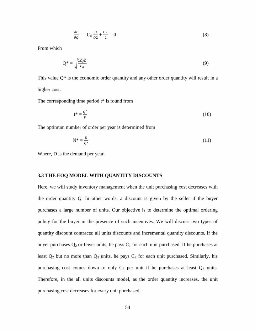
54

= - CS

+

= 0 (8)

From which

Q* = √

(9)

This value Q* is the economic order quantity and any other order quantity will result in a

higher cost.

The corresponding time period t* is found from

t* =

(10)

The optimum number of order per year is determined from

N* =

(11)

Where, D is the demand per year.

3.3 THE EOQ MODEL WITH QUANTITY DISCOUNTS

Here, we will study inventory management when the unit purchasing cost decreases with

the order quantity Q. In other words, a discount is given by the seller if the buyer

purchases a large number of units. Our objective is to determine the optimal ordering

policy for the buyer in the presence of such incentives. We will discuss two types of

quantity discount contracts: all units discounts and incremental quantity discounts. If the

buyer purchases Q2 or fewer units, he pays C1 for each unit purchased. If he purchases at

least Q2 but no more than Q3 units, he pays C2 for each unit purchased. Similarly, his

purchasing cost comes down to only C3 per unit if he purchases at least Q3 units.

Therefore, in the all units discounts model, as the order quantity increases, the unit

purchasing cost decreases for every unit purchased.

55

Figure 3.3 shows the total purchasing cost function for the all units discount.

TOTAL

COST

C1 C1/Unit C2/Unit

C2 C3/Unit

C3

Q2 Q3 Q4

ORDER QUANTITY (Q)

Figure 3.3: Total Purchasing Cost Function for the all units discount

The incremental quantity discount is an alternative type of discount. If the order quantity

is between Q2 and Q3, the unit purchasing price drops to C2 but only for units numbered

Q2 through Q3. Similarly, if at least Q4 units are purchased, the unit purchasing price

decreases to C3 for units above Q4.

Therefore, in the incremental quantity discounts case, the unit purchasing cost decreases

only for units beyond a certain threshold and not for every unit as in the all units

discounts case.

56

Figure 3.4 illustrates the total purchasing cost function.

TOTAL C3/Unit

COST

C2/Unit

C1/Unit

Q2 Q3 Q4

Order Quantity (Q)

Figure 3.4: Total purchasing costs for incremental quantity discount

Why are these discounts offered by suppliers? The reason is to make the customers

purchase more per order. Large orders result in high inventory holding costs because an

average unit spends a longer time in the system before it gets sold. Thus the seller’s price

discount subsidizes the buyer’s inventory holding cost.

We will begin with an analysis of the all units discounts contract. We want to find the

order quantity that minimizes the average annual sum of the purchasing, holding, and

fixed ordering costs.

3.3.1 All Units Discount

Similarly to the EOQ model, we assume that backordering is not allowed. Let m be the

number of discount possibilities. Let q1 = 0, q2, q3, . . . ,qj , qj+1, . . . ,qm be the order

quantities at which the purchasing cost changes. For simplicity in our analysis we will

57

assume from now on that units are infinitely divisible. The unit purchasing cost is the

same for all Q in (qj , qj+1); let the corresponding unit purchasing cost be denoted by Cj.

Thus, the jth

lowest unit purchasing cost is denoted by Cj; Cm is the lowest possible

purchasing cost with C1 being the highest unit purchasing cost.

The purchasing cost now depends on the value of Q. Hence our average annual cost is:

Zj(Q) = Cjλ + Kλ

+ ICj

, qj Q qj+1 (12)

Thus we have a family of cost functions indexed by the subscript j. The j th

cost function

is defined for only those values of Q that lie in (qj , qj+1).

These functions are shown in Figure 3.5.

Total Cost

C1/Unit

C2/Unit

C3/Unit

Q2 Q3 Q4

Figure 3.5: Total cost for all units discount.

The solid portion of each curve corresponds to the interval in which it is defined. The

average annual cost function is thus a combination of these solid portions.

Two observations can be made. First, the average annual cost function is not continuous.

58

It is segmented such that each segment is defined over a discount interval (qj , qj+1).

The segmented nature of the average annual cost function makes solving the problem

slightly more difficult since we now cannot simply take a derivative and set it to zero to

find the optimal solution.

It is the second observation that paves the way for an approach to find the optimal

solution. Different curves in Figure 3.5 are arranged in an order of decreasing unit

purchasing cost. The curve at the top corresponds to the highest per-unit purchasing cost

C1, and the lowest curve corresponds to the lowest per-unit purchasing cost Cm.

Also, the curves do not cross each other. To obtain the optimal solution, we will start

from the bottom-most curve which is defined for Q in (qm, ), and compute the lowest

possible cost in this interval. Then, in the second iteration, we will consider the second-

lowest curve and check to see if we could do better in terms of the cost.

The algorithm continues as long as the cost keeps decreasing. The steps of the algorithm

are outlined in the following subsection.

3.3.2 An Algorithm to Determine the Optimal Order Quantity for the All

Units Discount Case

Step 1: Set j = m. Compute the optimal EOQ for the mth cost curve, which we

denote by Q*m:

Q*m: = √ λ

(13)

Step 2: Is Q*m ≥ qm? If yes, Q*m is the optimal order quantity and we are done. If not,

the minimum cost occurs at Q = qm owing to the convexity of the cost function.

59

Since the minimum point Q*m < qm, the cost function for the mth

discount level is

increasing on the right of qm. Consequently, among all the feasible order quantities, that

is, for order quantities greater than or equal to qm, the minimum cost occurs at Q = qm.

Compute the cost corresponding to Q = qm. Let this cost be denoted by Zmin and

Qmin = qm and go to Step 3.

Step 3: Set j = j−1. Compute the optimal EOQ for the j th

cost curve:

Q*j: = √ λ

(14)

Step 4: Is Q*j in (qj , qj+1)? If yes, compute Z(Q*j) and compare with Zmin. If Z(Q*j)<

Zmin, Q*j is the optimal order quantity. Otherwise, Qmin is the optimal order quantity.

In either case, we are done.

Otherwise, if Q*j is not in (qj ,qj+1), then the minimum cost for the j th

curve occurs at Q

= qj owing to the convexity of the cost function. Compute this cost Z(qj). If

Z(qj) < Zmin, then set Qmin = qj and Zmin = Z(qj). If j ≥ 2, go to Step 3; otherwise,

stop.

3.3.3 Incremental Quantity Discount

The incremental quantity discount case differs from the all units discount case. In this

situation, as the quantity per order increases, the unit purchasing cost declines

incrementally on additional units purchased as opposed to on all the units purchased. Let

q1 = 0, q2, . . . ,qj ,qj+1, . . . ,qm be the order quantities at which the unit purchasing cost

changes. The number of discount levels is m. For our analysis we will assume that the

units are infinitely divisible and the purchasing quantity can assume any real value. The

60

unit purchasing cost is the same for all values of Q in (qj ,qj+1), and we denote this cost by

Cj. By definition, C1 >C2 >···>Cj >Cj+1 >···>Cm.

Our goal is to determine the optimal number of units to be ordered. We first write an

expression for the average annual purchasing cost if Q units are ordered.

Let Q be in the j th

discount interval, that is, Q lies between qj and qj+1. The purchasing

cost for Q in this interval is equal to

C(Q) =C1(q2 −q1)+C2(q3 −q2)+···+Cj−1(qj −qj−1)+Cj(Q−qj). (15)

Note that only the last term on the right-hand side of the above expression depends on

Q.

Let Rj be used to denote the sum of the terms that are independent of Q. That is,

Rj =C1(q2 −q1)+C2(q3 −q2)+···+Cj−1(qj −qj−1), j ≥ 2, with R1 = 0. (16)

Therefore,

C(Q) = Rj + Cj (Q−qj). (17)

Now the average unit purchasing cost for Q units is equal to

, which is equal to

=

+ Cj - Cj

(18)

The average annual purchasing cost when each order consists of Q units is equal to

λ. The fixed order cost and holding cost terms remain similar to those in the basic

EOQ model except that the average annual holding cost per unit is now equal to I

This is not surprising since the holding cost per unit depends on the cost of each unit,

which is a function of the order size given the cost structure here. The average annual

cost of managing inventory is thus equal to

Z(Q) =

λ + K

λ

+

(19)

61

Z(Q) = (

+ Cj - Cj

) λ + K

λ

+

–

) (20)

Realigning terms yields

Z(Q) = Cj λ + (Rj – Cjqj +K)λ

+

+

–

(21)

Which is valid for qj ≤ Q < qj+1.

Figure 3.6 shows the Z(Q) function. Once again, we have a family of curves, each of

which is valid for a given interval. The valid portion is shown using a solid line. Thus the

curve with the solid line constitutes the Z(Q) function. Unlike the all units discount cost

function, Z(Q) is a continuous function. It turns out that the optimal solution Q* cannot

be equal to any one of {q1,q2, . . . ,qm,qm+1}.

Total Cost

Q1 Q2 Q3

Order Quantity (Q)

Figure 3.6: The Z(Q) Function

We use this fact to construct an algorithm to determine the optimal order quantity.

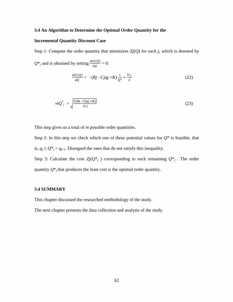
62

3.4 An Algorithm to Determine the Optimal Order Quantity for the

Incremental Quantity Discount Case

Step 1: Compute the order quantity that minimizes Zj(Q) for each j, which is denoted by

Q*j and is obtained by setting

= 0:

= −(Rj −Cjqj +K)

λ

+

(22)

⇒Q*j = √

(23)

This step gives us a total of m possible order quantities.

Step 2: In this step we check which one of these potential values for Q* is feasible, that

is, qj ≤ Q*j < qj+1. Disregard the ones that do not satisfy this inequality.

Step 3: Calculate the cost Zj(Q*j ) corresponding to each remaining Q*j . The order

quantity Q*j that produces the least cost is the optimal order quantity.

3.4 SUMMARY

This chapter discussed the researched methodology of the study.

The next chapter presents the data collection and analysis of the study.

63

CHAPTER FOUR

DATA COLLECTION AND ANALYSIS

4.0 INTRODUCTION

In this chapter, we shall analyzed a company’s inventory control problem and apply our

proposed method in solving our problem.

The aim is to determine the maximum discount price that should be taken, and the

quantity that should be ordered giving the quantity discount. The general practice is that

most establishments do not analyze the quantity discount that companies offered them

with their carrying cost. They either go for it or reject it by the discretion of people or

departments in charge. These are basically inefficient as carrying cost may be high or

low.

4.1 DATA COLLECTION AND ANALYSIS

Suppliers of Non-Security Examination Materials to The West African Examinations

Council (WAEC), occasionally give discounts to WAEC in line with its organizational

policy in order to reduce a large stock of its materials which may increase its holding

cost.

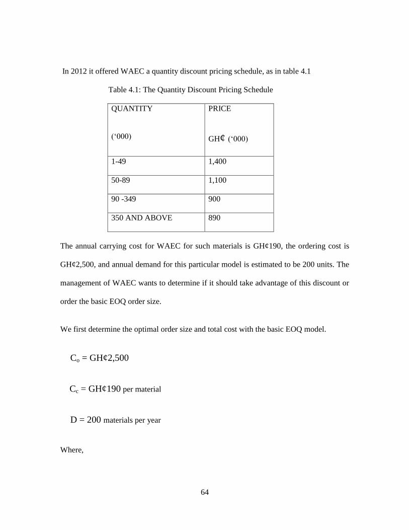
64

In 2012 it offered WAEC a quantity discount pricing schedule, as in table 4.1

Table 4.1: The Quantity Discount Pricing Schedule

QUANTITY

(‘000)

PRICE

GH¢ (‘000)

1-49 1,400

50-89 1,100

90 -349 900

350 AND ABOVE 890

The annual carrying cost for WAEC for such materials is GH¢190, the ordering cost is

GH¢2,500, and annual demand for this particular model is estimated to be 200 units. The

management of WAEC wants to determine if it should take advantage of this discount or

order the basic EOQ order size.

We first determine the optimal order size and total cost with the basic EOQ model.

Co = GH¢2,500

Cc = GH¢190 per material

D = 200 materials per year

Where,

65

Co = the Ordering Cost

Cc = Carrying Cost

D = annual demand

P = Price

Qopt = Optimal Quantity

Qopt = √

(24)

= √

(25)

= 72.5 materials

Although we will use Qopt = 72.5 in the subsequent computations, realistically the order

size would be 73 materials. This order size is eligible for the first discount of

GH¢1,100; therefore, this price is used to compute total cost:

TCmin =

+

+ PD (26)

=

+

+ (1,100) (200)

66

TCmin = GH¢233,784

Since there is a discount for a larger order size than 50 units, this total cost of must be

compared with total cost with an order size of 90 and a discounted price of GH¢900:

TC =

+

+ PD (27)

=

+

+ (900) (200)

= GH¢194,105

Since there is a discount for a larger order size than 90 units this total cost of must be

compared with total cost with an order size of 350 and a discounted price of GH¢890:

TC =

+

+ PD (28)

=

+

+ (890) (200)

= GH¢212,678.57

4.2 RESULTS

The maximum discount price that gave lowest cost was GH¢900 at a minimum quantity

of 90,000.

67

Even though this total cost is lower among all the total costs, the maximum discount price

of GH¢900 should not be taken at the required quantity range of 90,000-349,000 units

should be ordered. The reason being that, if institution such as WAEC goes for the

discount at that minimum levels it might not meet its quantity obligation to satisfy the

total number of candidature. In this case or situation, the next discount price of GH¢890

is considered at a minimum quantity of 350. We observed that there is no order size

larger than 350 that would result in a lower cost.

4.3 CONCLUSIONS

In the EOQ model, the cost of capital considerations must be captured by a proper

estimate of the situations, there is no need for the special rate-of-return analysis. If any

rate of return analysis is to be done, it must be done by method to ensure that the cost of

capital is not double counted. Even though it is necessary that companies begin to

estimate their carrying cost factor correctly, this alone at times cannot be sorely used to

decide whether the company should go for a discount price that gave the minimum cost.

If they do, their calculated EOQs inventory carrying costs. If they are not, the computed

EOQ itself will be suboptimal. On the other hand, as long as the cost of capital

considerations are so captured, even in quantity discount may not always be the true

EOQs and their analysis of the quantity discount situation with the traditional approach

will result in sub optimal decisions. What that particular item is going to be used for the

required number needed must also be considered before decisions are made, as in the

case above.

68

By applying our EOQ model to the company’s problem, it was observed that the solution

that gave maximum achievable value was GH¢890 at a quantity of 350.

Management may benefit from the proposed approach for the organization’s inventory

decision making. We therefore recommend that the model should be adopted by the

company for its inventory control management.

69

CHAPTER FIVE

CONCLUSIONS AND RECOMMENDATIONS

5.0 INTRODUCTION

In quantity discount situations, the traditional economic order quantity (EOQ) model’s

approach is to accept the discount if the total annual costs of inventory ordering, carrying

and purchase with the discount are lower than those costs without the discount. This may

not necessarily be the case in certain instances since this approach could lead to the

acceptance of a discount that actually lead to increased inventory carrying cost. Our

research focused on the use of the EOQ model with quantity discount for determining

whether the company should accept the discount that is offered, and at what quantity

must it order at that discount for a particular company in Ghana. It can however be

applied to any institution which handles material requisition.

5.1 CONCLUSIONS

This thesis seeks to solve a real-life problem of a Company in Ghana EOQ model with

quantity discount. It was observed that the solution that gave maximum achievable value

was GH¢890 at a quantity of 350. This means that the company should spend a total cost

of eight hundred and ninety thousand Ghana cedis (GH¢890,000) to order an optimal

quantity of three hundred and fifty thousand (350,000) unit of material.

From available records, there is no such method for determining what quantity discount

level the quantity should place its order and just accept the minimum discounts as per the

70

decision of the department in charge, which always lead to shortage of materials

procured.

For the data used for our analysis, the company using their approach arrived at the

discount price of GH¢890 at a quantity of 350.

5.2 RECOMMENDATIONS

The use of computer application in computation gives a systematic and transparent

solution as compared with an arbitrary method. Using the more scientific model for the

inventory management of the company’s inventory control system gives a better result.

Management may benefit from the proposed approach for their inventory control

management system and could help them take informed decision. We therefore

recommend that our model should be adopted by the company for their inventory control

and management planning.

71

REFERENCES:

Ben-Daya M. (1999). Multi-stage lot sizing models with imperfect processes and

inspection errors. Production Planning & Control, vol. 10, no.2, 118-126.

Chan, Ibrahim, & Lochert. (2003). A new EPQ model: integrating lower pricing, rework

and reject situation. Production Planning and Control, vol. 14, no. 7, 588-595.

Chang C T. (2002). Extended economic quantity model under cash discount and payment

delay. Information and Management Science, 13(3),57-69.

Chang, Yao, & Lee. (1998). Economics reorder point for fuzzy backorder quantity.

European Journal of Operational Research, 183-202.

Chen & Wang. (1996). Backorder fuzzy inventory model under functional principle.

Information Science, 71-79.

Chen Y C. (2003). A probabilistic approach for traditional EOQ model . Journal of

Information Optimisation Sciences, 24(2), 249-253.

Chiu Y P. (2003). Determining the optimal lot size for the finite production model with

random defective rate, the rework and bscklogging. Engineering Optimisation,

vol. 35, no.4, 427-437.

Goyal S K. (1985). Economic Order Quantity under Conditions of Permissible Delay in

Payments. Operational Research Society, 36(4),335-335.

Goyal, Huang, & Chen, &. (2003). A simple integrated production policy of an imperfect

item for vendor and buyer. Production Planning & Control, vol. 14, no. 7, 596-

602.

72

Halim, Giri, & Chaudhuri. (2008). Fuzzy economic order quantity model for perishable

items with stochastic demand, partial backlogging and fuzzy deteriorating rate.

International Journal of Operational Research, 3,77-96.

Harris F W. (1915). Operation and cost, The librarg of Factory Management. Chicago:

Pearson.

Lee & Yao. (1998). Economic production quantity for demand quantity and fuzzy

production quantity. European Journal of Operational Research, 109, 203-211.

Liberatore M J. (1979). The EOQ model under stochastic lead time. Operations

Research, 27, 391-396.

Lin & Yao. (2000). Fuzzy economic production for production inventory. Fuzzy Sets and

Systems, 111, 465-495.

Liu B. (2007). Uncetainty Theory, 2nd ed. Washington: Springer-Verlag.

Liu B. (2010). Uncertainty Theory: A branch of mathematics for modeling human

uncertainty. Washington: Springer-Verlag.

Makis & Fung. (1998). An EMQ model with inspections and random machine failures.

Journal of the Operational Research Society, vol. 49, no. 1, 66-76.

Moon S L. (2000). The effects of inflation and time-value of money on an economic

order quantity model with a random product life cycle. European Journal of

Operational Research, 125(3), 588-601.

Ouyang & Chang. (2000). Impact of investing in quality improvement on (Q, r, L) model

involving the imperfect production proccess. Production Planning & Control, vol.

11, no. 6, 598-607.

73

Ouyang & Yao. (2002). A minimax distribution free procedure for mixed inventory

model involving variable lead time with fuzzy demand. Computers and

Operations Research, 29, 471-487.

Ouyang, Chen, & & Chang. (2002). Quality improvement,setup cost and lead-time

reductions in lot size reorder point models with an imperfect production process.

Computers & Operations Research, vol. 29, 1701-1717.

Ouyang, Wu, & Ho. (2003). The integrated inventory models with defective items and

controllable lead time. Production Planning & Control, vol. 14, no. 7, 562-578.

Park K S. (1987). Fuzzy set theoritic interpretation of economic order quantity. IEEE

Transaction on Systems, Man and Cybemetrics, 17(6),1080-1084.

Parler & Wang. (1993). Diversification under yield randomness in inventory models.

European Journal of Operarion Research, 66(1),52-64.

Porteus E L. (1986). Optimal lot sizing, process quality improvement and setup cost

reduction. Operational Research Journal, vol. 34, 137-144.

Rosenblat & Lee. (1986). Economic production cycles with imperfect production

processes. IIE Transaction, Vol. 18, 48-55.

Rosenblatt & Lee. (1987). Simultaneous deermination of production cycles and

inspection schedules in a production system. Management Science, vol. 33, 1125-

1137.

Roy & Maiti. (1997). A fuzzy EOQ model with demand dependent unit cost under

limited storage capacity. European Journal of Operational Research, 99,425-432.

Salameh & Jaber. (2000). Economic production quantity model for items with imperfect

quality. International Journal of Production Economics, vol. 64, 59-64.

74

Soumen, Debjani, & Roy. (2009). A production inventory model with fuzzy random

demand and with flexible and reliability considerations. Computers and Industrial

Engineering, 56(1),411-416.

Teng J T. (2002). On the economic order quality under conditions of permissible delay in

payment. Operational Research Society, 53, 915-918.

Teng, Yang, & Ouyang. (2003). On an EOQ model for deteriorating items with time-

varying demand and partial backlogging. Journal of the Operational Research

Society, 54, 432-436.

Urban T L. (1992). Deterministic inventory models incorporation marketing decisions.

Computers and Industrail Engineering, vol. 22, no. 1, 85-93.

Vijayan & Kumaran. (2009). Fuzzy economic order time models with random demand.

International Jounal of Approximately Reasoning, 50,529-540.

Vujosevic & Petrovic. (1996). EOQ formula when inventory cost is fuzzy. Inventory

HJournal of Production Economics, 45, 499-504.

Wang, Tang, & Xue. (2006). Fuzzy random EOQ model with imperfect quality items.

Machine Learning and Cybernetics.

Wang, Tang, & Zhao. (2007). Fuzzy economic order quantity inventory without

backordering. Tsinghua Science and Technology, 21(1), 91-96.

Wang, Tang, & Zhao. (2007). Random fuzzy EOQ model with imperfect quality items.

Fuzzy Optimal Decision Making, 6, 139-153.

Yao, Chang, & Su. (2000). Fuzzy inventory without backorder for fuzzy order quantity

and fuzzy total demand quantity. Computer and Operations Research, 27,935-

962.

75

Yu, Zhao, & Su. (2006). Extended newsboy problem based on fuzzy random demand.

System Engineering, 24(9),103-107.

Zhang & Gerchak. (1990). Joint lot sizing and inspection policy in an EOQ model with

random yield. IIE Transactions, vol. 22, no. 1, 41-47.