APPLICATION OF BACTERIAL BIOFLOCCULANTS FOR WASTEWATER AND ...
301
APPLICATION OF BACTERIAL BIOFLOCCULANTS FOR WASTEWATER AND RIVER WATER TREATMENT Simphiwe P. Buthelezi Submitted in fulfilment of the academic requirements for the degree of Master of Science in the Discipline of Microbiology, School of Biochemistry, Genetics, Microbiology and Plant Pathology, Faculty of Science and Agriculture at the University of KwaZulu-Natal, Durban. As the candidate’s supervisor, I have approved this dissertation for submission. Signed: Name: Date:
Transcript of APPLICATION OF BACTERIAL BIOFLOCCULANTS FOR WASTEWATER AND ...
APPLICATION OF BACTERIAL BIOFLOCCULANTS FOR WASTEWATER
AND RIVER WATER TREATMENT
Simphiwe P. Buthelezi
Submitted in fulfilment of the academic requirements for the degree of Master of
Science in the Discipline of Microbiology, School of Biochemistry, Genetics,
Microbiology and Plant Pathology, Faculty of Science and Agriculture at the
University of KwaZulu-Natal, Durban.
As the candidate’s supervisor, I have approved this dissertation for submission.
Signed: Name: Date:

For my parents: Mr and Mrs E. Buthelezi
Declaration by the candidate This MSc study was carried out in the School of Biochemistry, Genetics, Microbiology and Plant Pathology, University of KwaZulu-Natal, Westville Campus, under the supervision of Professor B Pillay. 1. The research reported in this dissertation, except where otherwise indicated, is my
original research. 2. This dissertation has not been submitted for any degree or examination at any
other university. 3. This dissertation does not contain other scientists’ data, pictures, graphs or other
information, unless specifically acknowledged as being sourced from other scientists.
4. This dissertation does not contain other scientists’ writing, unless specifically
acknowledged as being sourced from other scientists. Where other written sources have been quoted, then their words have been re-written but the general information attributed to them has been referenced.
5. This dissertation does not contain text, graphics or tables taken from the Internet,
unless specifically acknowledged, and the source being detailed in the dissertation and in the References section.
………………………………………………….....
Simphiwe Promise Buthelezi (Candidate)
i
ACKNOWLEDGEMENTS
The author records her appreciation to the following persons and organizations for their
assistance in the completion of this study:
Prof. B. Pillay, Department of Microbiology, University of KwaZulu-Natal for his
contribution, supervision, academic stimulation and words of encouragement;
Prof. J. Lin for his support and words of encouragement;
Dr. A. O. Olaniran for his assistance and support;
Dr. R. Shaik for her assistance and support;
Dr. M. E. Setati for her assistance and support;
Mr A. Govender for his assistance and support;
Mr. K. Buthelezi, Mr. L. Buthelezi, Mrs E. Buthelezi, Mr and Mrs Simpson, Mrs Z.
Zungu, Mrs D. N. Ngubane, Miss M. Makatini, Mr. G. Makaula, Mr. I. Karodia, Mr. B.
Naidoo, Mr. S. Dlamini, Mr. L. Mnguni, Mr and Mrs Mnyeni, and Mr. M. Ngiba for their
support;
LIFElab, DAAD and the UKZN for financial assistance;
Staff and postgraduate students of the Discipline of Microbiology (Westville campus),
University of KwaZulu-Natal, for their companionship and selfless assistance;
God, for being with me throughout the course of the study;

ii
Family and friends for their support, emotional and spiritual strength throughout the
course of the study.
iii
ABSTRACT
Dyes are often recalcitrant organic molecules that produce a colour change and contribute
to the organic load and toxicity of textile industrial wastewater. Untreated effluent from
such sources is harmful to aquatic life in the rivers and lakes due to reduced light
penetration and the presence of highly toxic metal complex dyes. The use of alum as
flocculant/coagulant in wastewater treatment is not encouraged as it induces Alzheimer’s
disease in humans and results in the production of large amounts of sludge. Therefore, the
development of safe and biodegradable flocculating agents that will minimize
environmental and health risks may be considered as an important issue in wastewater
treatment. Bioflocculants are extracellular polymers synthesized by living cells. In this
study, bacterial bioflocculants were assessed for their ability to remove dyes from textile
wastewater as well as reducing the microbial load in untreated river water. The bacteria
were isolated from a wastewater treatment plant and identified using standard
biochemical tests as well as the analysis of their 16S rDNA gene sequences. Six bacterial
isolates were identified viz. Staphylococcus aureus, Pseudomonas plecoglossicida,
Pseudomonas pseudoalcaligenes, Exiguobacterium acetylicum, Bacillus subtilis, and
Klebsiella terrigena. The flocculating activities of the bioflocculants produced by these
isolates were characterized. The effect of temperature, pH, cations and bioflocculant
concentration on the removal of dyes, kaolin clay and microbial load was also
determined. The amount of bioflocculants produced by the bacterial isolates ranged
between 5 and 27.66 g/l. According to the findings of the present study, bacterial
bioflocculants were composed of carbohydrates, proteins, uronic acid, and hexosamine in
varying quantities. The bioflocculants were effective to varying degrees in removing the
dyes in aqueous solution, in particular whale dye, medi-blue, fawn dye and mixed dyes,
with a decolourization efficiency ranging between 20-99.9%. Decolourization efficiency
was influenced by the bioflocculant concentration, pH, temperature, and cations. The
bacterial bioflocculants were also capable of reducing both the kaolin clay and the
microbial load from river water. The flocculating activity ranged between 2.395–3.709
OD-1 while up to 70.84% of kaolin clay and 99% of the microbial load from the river
water was removed. The efficiency of kaolin clay flocculation increased with higher
iv
concentration of bacterial bioflocculants. The optimum pH for the flocculating activity
was observed between 6 and 9. The best flocculating activity was observed at 28oC.
Divalent cations such as Mg2+ and Mn2+ improved the flocculation while salts such as
K2HPO4, CH2COONa, and Na2CO3 did not. The findings of this study strongly suggest
that microbial bioflocculants could provide a promising alternative to replace or
supplement the physical and chemical treatment processes of river water and textile
industry effluent.
v
LIST OF FIGURES
Page
Fig. 1.1: Scheme of operations involved in textile cotton industry and the main
pollutants from each step (Dos Santos et al., 2007). 2
Fig. 1.2: The water cycle (http://www.usgcrp.gov/usgcrp/images/ocp2003/Water
Cycle optimized.jpg). 8
Fig. 1.3: Production of methane on a small scale (Nester et al., 2001). 11
Fig. 1.4: Major steps involved in modern sewage treatment plants
(http://web.deu.edu.tr/atiksu/toprak/summary4.html). 13
Fig. 1.5: Proposed mechanism for reduction of azo dyes by whole bacterial cells
(Keck et al., 1997). 19
Fig. 1.6: (a) The structure of the exopolysaccharide from Xanthomonas campestris
pv campestris (xanthan). (b) The structure of gellan from
Sphingomonas paucimobilis (Sutherland, 1998). 23
Fig. 2.1: PCR products after amplification of the 16S rDNA sequences of the
bacterial isolates. Lanes 1−6: E1; A17; D1; A22; R2; A14;and
lane 7: Molecular weight marker VI (Roche Biochemicals). 38
Fig. 2.2: Bioflocculant produced by the bacterial isolates 39
Fig. 2.3: Carbohydrate and protein content of the bacterial bioflocculants. 40
Fig. 2.4: Uronic acid content of the bacterial bioflocculants. 41
vi
Fig. 2.5: Amino sugar content of the bacterial bioflocculants. 41
Fig. 3.1: Growth patterns of the bacterial isolates in YMPG medium. 54
Fig. 3.2: Effect of time on the flocculating activity of crude bioflocculants using
a kaolin suspension. 55
Fig. 3.3: Effect of time on the removal of a kaolin suspension by crude
bioflocculants. 55
Fig. 3.4: Flocculating activity of the bacterial bioflocculants using a kaolin
suspension. 56
Fig. 3.5: Flocculating activity of bacteria by their bioflocculants. 57
Fig. 3.6: Flocculation of microbial cultures using bacterial bioflocculants. 58
Fig. 3.7: Effect of flocculant concentration on the flocculating activity with
respect to 10 ppm alum using pond water. Symbols: �, 10 ppm; �,
20 ppm4; �, 30ppm; �, 50 ppm. 60
Fig. 3.8: Effect of pH on the flocculating activity of bacterial biofloccunts. 61
Fig. 3.9: Effect of temperature on the flocculating activity of bacterial
bioflocculants. Symbols: �, 37oC; �, 28oC. 61
Fig. 3.10: Effect of cationic compounds on the flocculating activity of bacterial
bioflocculants. Symbols: �, CTAB; �, MgSO4; �, MnCl2; �, CaCl2. 62
Fig. 4.1: Effect of flocculant concentration on the removal of whale dye. 75
vii
Fig. 4.2: Flocculation of whale dye by the bacterial bioflocculants. 75
Fig. 4.3: Effect of pH on the removal of whale dye at 10 ppm. 76
Fig. 4.4: Effect of temperature on the removal of whale dye at 10 ppm.
Symbols: �, 28oC; �, 35oC; �, 40oC; �, 45oC. 77
Fig. 4.5: Effect of cations on the removal of whale dye at 10 ppm.
Symbols: �, CTAB; �, CaCl2; �, MnCl2; �, MgSO4. 77
Fig. 4.6: Effect of flocculant concentration on the removal of medi-blue dye. 78
Fig. 4.7: Flocculation of medi-blue dye by the bacterial bioflocculants. 79
Fig. 4.8: Effect of pH on the removal of medi-blue dye at 10 ppm. 80
Fig. 4.9: Effect of temperature on the removal of medi-blue dye at10 ppm.
Symbols: �, 28oC; �, 35oC; �, 40oC; �, 45oC. 81
Fig. 4.10: Effect of cations on the removal of medi-blue dye at 10 ppm.
Symbols: �, CTAB; �, CaCl2; �, MnCl2; �, MgSO4. 81
Fig. 4.11: Effect of flocculant concentration on the removal of fawn dye. 82
Fig. 4.12: Flocculation of fawn dye by the bacterial bioflocculants. 83
Fig. 4.13: Effect of pH on the removal of fawn dye at 10 ppm. 84
Fig. 4.14: Effect of temperature on the removal of fawn dye at 10 ppm.
Symbols: �, 28oC; �, 35oC; �, 40oC; �, 45oC. 84
viii
Fig. 4.15: Effect of cations on the removal of fawn dye at 10 ppm.
Symbols: �, CTAB; �, CaCl2; �, MnCl2; �, MgSO4. 85
Fig. 4.16: Effect of flocculant concentration on the removal of mixed dyes. 86
Fig. 4.17: Flocculation of mixed dyes by the bacterial bioflocculants. 86
Fig. 4.18: Effect of pH on the removal of mixed dyes at 10 ppm. 87
Fig. 4.19: Effect of temperature on the removal of mixed dyes at 10 ppm.
Symbols: �, 28oC; �, 35oC; �, 40oC; �, 45oC. 88
Fig. 4.20: Effect of cations on the removal of mixed dyes at 10 ppm.
Symbols: �, CTAB; �, CaCl2; �, MnCl2; �, MgSO4. 88
Fig. 5.1: Effect of bacterial biofflocculants and alum on the turbidity of river water
at 10 ppm. 100
Fig. 5.2: Effect of bacterial biofflocculants and alum on the turbidity of river water
at 50 ppm. 100
Fig. 5.3: Flocculating activity of the bacterial bioflocculants at different time
intervals with E. coli. 101
Fig. 5.4: pH of the river water before and after the addition of the bacterial
bioflocculants and alum. 101
Fig. 5.5: Effect of bioflocculant concentration and alum on the reduction of river
water turbidity. 102
ix
Fig. 5.6: Flocculating activity of bioflocculants compared to alum using river
water. 103
Fig. 5.7: Effect of bioflocculant concentration and alum on the microbial load
in river water. 103
Fig. 5.8: The effect of pH on the reduction of river water turbidity by the bacterial
bioflocculants at different concentrations compared to alum. 104
Fig. 5.9: The effect of pH on the flocculating activity of the bacterial bioflocculants
compared to alum. 105
Fig. 5.10: The effect of pH on the reduction of the microbial load by the
bioflocculants at different concentrations compared to alum. 105
Fig. 5.11: The reduction of river water turbidity spiked with two Gram-positive
and Gram negative bacteria by the bacterial bioflocculants compared
to alum at 10 ppm (Strep = S. faecalis, Staph = S. aureus, Kleb =
K. oxytoca, E. coli = E. coli). 107
Fig. 5.12: The reduction of river water turbidity spiked with two Gram-positive
and Gram-negative bacteria by the bacterial bioflocculants compared
to alum at 50 ppm (Strep = S. faecalis, Staph = S. aureus, Kleb =
K. oxytoca, E. coli = E. coli). 107
Fig. 5.13: Flocculating activity of bioflocculants compared to alum using
river water spiked with two Gram-positive and Gram-negative
bacteria (Strep = S. faecalis, Staph = S. aureus, Kleb =
K. oxytoca, E. coli = E. coli) 108
x
Fig. 5.14: The reduction of the microbial load by the bioflocculants at different
concentrations compared to alum at 10 ppm (Strep = S. faecalis,
Staph = S. aureus, Kleb = K. oxytoca, E. coli = E. coli). 108
Fig. 5.15: The reduction of the microbial load by the bioflocculants at different
concentrations compared to alum at 50 ppm (Strep = S. faecalis,
Staph = S. aureus, Kleb = K. oxytoca, E. coli = E. coli). 109
xi
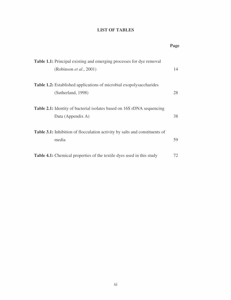
LIST OF TABLES
Page
Table 1.1: Principal existing and emerging processes for dye removal
(Robinson et al., 2001) 14
Table 1.2: Established applications of microbial exopolysaccharides
(Sutherland, 1998) 28
Table 2.1: Identity of bacterial isolates based on 16S rDNA sequencing
Data (Appendix A) 38
Table 3.1: Inhibition of flocculation activity by salts and constituents of
media 59
Table 4.1: Chemical properties of the textile dyes used in this study 72
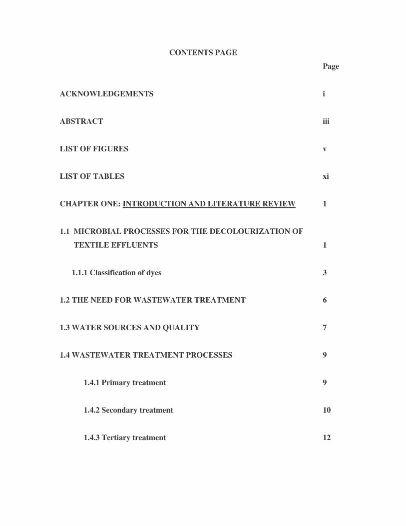
CONTENTS PAGE
Page
ACKNOWLEDGEMENTS i
ABSTRACT iii
LIST OF FIGURES v
LIST OF TABLES xi
CHAPTER ONE: INTRODUCTION AND LITERATURE REVIEW 1
1.1 MICROBIAL PROCESSES FOR THE DECOLOURIZATION OF
TEXTILE EFFLUENTS 1
1.1.1 Classification of dyes 3
1.2 THE NEED FOR WASTEWATER TREATMENT 6
1.3 WATER SOURCES AND QUALITY 7
1.4 WASTEWATER TREATMENT PROCESSES 9
1.4.1 Primary treatment 9
1.4.2 Secondary treatment 10
1.4.3 Tertiary treatment 12
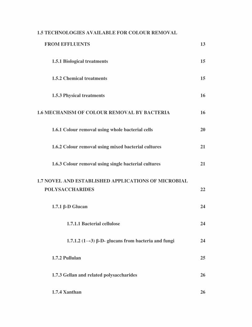
1.5 TECHNOLOGIES AVAILABLE FOR COLOUR REMOVAL
FROM EFFLUENTS 13
1.5.1 Biological treatments 15
1.5.2 Chemical treatments 15
1.5.3 Physical treatments 16
1.6 MECHANISM OF COLOUR REMOVAL BY BACTERIA 16
1.6.1 Colour removal using whole bacterial cells 20
1.6.2 Colour removal using mixed bacterial cultures 21
1.6.3 Colour removal using single bacterial cultures 21
1.7 NOVEL AND ESTABLISHED APPLICATIONS OF MICROBIAL
POLYSACCHARIDES 22
1.7.1 �-D Glucan 24
1.7.1.1 Bacterial cellulose 24
1.7.1.2 (1�3) �-D- glucans from bacteria and fungi 24
1.7.2 Pullulan 25
1.7.3 Gellan and related polysaccharides 26
1.7.4 Xanthan 26
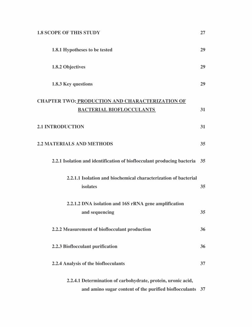
1.8 SCOPE OF THIS STUDY 27
1.8.1 Hypotheses to be tested 29
1.8.2 Objectives 29
1.8.3 Key questions 29
CHAPTER TWO: PRODUCTION AND CHARACTERIZATION OF
BACTERIAL BIOFLOCCULANTS 31
2.1 INTRODUCTION 31
2.2 MATERIALS AND METHODS 35
2.2.1 Isolation and identification of bioflocculant producing bacteria 35
2.2.1.1 Isolation and biochemical characterization of bacterial
isolates 35
2.2.1.2 DNA isolation and 16S rRNA gene amplification
and sequencing 35
2.2.2 Measurement of bioflocculant production 36
2.2.3 Bioflocculant purification 36
2.2.4 Analysis of the bioflocculants 37
2.2.4.1 Determination of carbohydrate, protein, uronic acid,
and amino sugar content of the purified bioflocculants 37
2.3 RESULTS 37
2.3.1 Bacterial isolation and identification 37
2.3.2 Measurement of bioflocculant production 39
2.3.3 Purification and analysis of the composition of the bacterial
bioflocculants 39
2.3.3.1 Carbohydrate and protein 40
2.3.3.2 Uronic acid and Amino sugars 40
2.4 DISCUSSION 42
CHAPTER THREE: COAGULATION-FLOCCULATION BY MICROBIAL
BIOFLOCCULANT 46
3.1 INTRODUCTION 46
3.2 MATERIALS AND METHODS 51
3.2.1 Determination of the growth patterns of bacterial
isolates and measurement of flocculating activity 51
3.2.2 Flocculation of microbial cultures 51
3.2.3 Flocculation inhibition assay 52
3.2.4 Flocculating activities of bacterial bioflocculants and alum 52
3.2.5 Determination of the effect of pH, temperature, and cationic/
metal salts on the flocculating activity of bioflocculants 53
3.3 RESULTS 53
3.3.1 The growth patterns of the bacterial isolates in YMPG media
and flocculating activities 53
3.3.2 Flocculation of microbial cultures 56
3.3.3 Inhibition of flocculating activity 57
3.3.4 Comparison of flocculating activities between bacterial
bioflocculants and alum 58
3.3.5 Effect of pH, temperature and cationic compounds on
flocculating activity 60
3.4 DISCUSSION 62
CHAPTER FOUR: MICROBIAL DECOLOURIZATION OF EFFLUENTS
CONTAINING TEXTILE-DYES 67
4.1 INTRODUCTION 67
4.2 MATERIALS AND METHODS 71
4.2.1 Textile dyes used in this study 71
4.2.2 Sample collection 72
4.2.3 Effect of flocculant concentration on dye removal 73
4.2.4 Effect of pH on dye removal 73
4.2.5 Effect of temperature on dye removal 73
4.2.6 Effect of cations on dye removal 74
4.3 RESULTS 74
4.3.1 Effect of flocculant concentration on the flocculating activity
and the removal of whale dye 74
4.3.2 Effect of pH, temperature, and cations on the removal of whale
dye 76
4.3.3 Effect of flocculant concentration on the flocculating activity
and the removal of medi-blue dye 78
4.3.4 Effect of pH, temperature, and cations on the removal of the
medi-blue dye 79
4.3.5 Effect of flocculant concentration on the flocculating activity
and the removal of fawn dye 82
4.3.6 Effect of pH, temperature, and cations on the removal of fawn
dye 83
4.3.7 Effect of flocculant concentration on the flocculating activity
and the removal of mixed dyes 85
4.3.8 Effect of pH, temperature, and cations on the removal of mixed
dyes 87
4.4 DISCUSSION 89
CHAPTER FIVE: THE TREATMENT OF RIVER WATER BY THE
BIOFLOCCULANTS 93
5.1 INTRODUCTION 93
5.2 MATERIALS AND METHODS 96
5.2.1 Microbiological analysis of river water 96
5.2.2 Determination of flocculating activity 97
5.2.3 Reduction of river water turbidity and microbial load 98
5.2.4 Effect of pH on decreasing the microbial load 98
5.3 RESULTS 99
5.3.1 Microbiological analysis of river water 99
5.3.2 The reduction of river water turbidity by the bacterial
bioflocculants and the flocculating activities 99
5.3.3 Effect of bioflocculants on river water turbidity and microbial
load 102
5.3.4 Effect of pH on decreasing the microbial load 104
5.3.5 Effect of bioflocculants on river water spiked with bacteria 106
5.4 DISCUSSION 109
CHAPTER SIX: CONCLUDING REMARKS 114
6.1 THE RESEARCH IN PERSPECTIVE 114
6.2 POTENTIAL FOR FUTURE DEVELOPMENT OF THIS WORK 116
REFERENCES 118
APPENDIX A: 16S rDNA sequences 146
APPENDIX B: Data 148
1
CHAPTER ONE
INTRODUCTION AND LITERATURE REVIEW
A great number of industries such as textile, paper and pulp, printing, iron-steel,
coke, petroleum, pesticide, paint, solvent, pharmaceutics, wood preserving chemicals,
consume large volumes of water and organic based chemicals. These chemicals show a
vast difference in chemical composition, molecular weight, and toxicity. Effluents from
these industries may also contain undesired quantities of these pollutants and need to be
treated (Aksu, 2005).
1.1 MICROBIAL PROCESSES FOR THE DECOLOURIZATION OF TEXTILE
EFFLUENTS
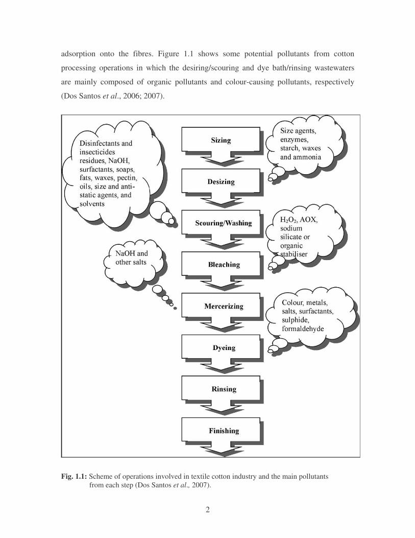
The most common textile-processing set-up (Fig. 1.1) for the decolourization of
textile effluents consists of desizing, scouring, bleaching, mercerising, and dyeing
processes (Dos Santos et al., 2007). Sizing is the first preparation step, which involves
the addition of sizing agents such as starch, polyvinyl alcohol (PAVE) and
carboxymethyl cellulose. These agents provide strength to the fibres and minimize
breakage. Desizing is employed next, to remove sizing materials prior to weaving.
Scouring removes impurities from the fibres by using alkali solution (commonly sodium
hydroxide) to breakdown natural oils, fats, waxes and surfactants, as well as to emulsify
and suspend impurities in the scouring bath. Bleaching is the step used to remove
unwanted colour from the fibres by using chemicals such as sodium hypochlorite and
hydrogen peroxide. Bleaching is followed by mercerising which is a continuous chemical
process used to increase dye-ability, lustre, and fibre appearance. In this step, a
concentrated alkaline solution is applied and an acid solution washes the fibres before the
dyeing step. Finally, dyeing is the process of adding colour to the fibres, which normally
requires large volumes of water not only in the dye bath, but also during the rinsing step.
Depending on the dyeing process, many chemicals like metals, salts, surfactants, organic
processing assistants, sulphide and formaldehyde, may be added to improve dye
2
adsorption onto the fibres. Figure 1.1 shows some potential pollutants from cotton
processing operations in which the desiring/scouring and dye bath/rinsing wastewaters
are mainly composed of organic pollutants and colour-causing pollutants, respectively
(Dos Santos et al., 2006; 2007).
Fig. 1.1: Scheme of operations involved in textile cotton industry and the main pollutants from each step (Dos Santos et al., 2007).
3
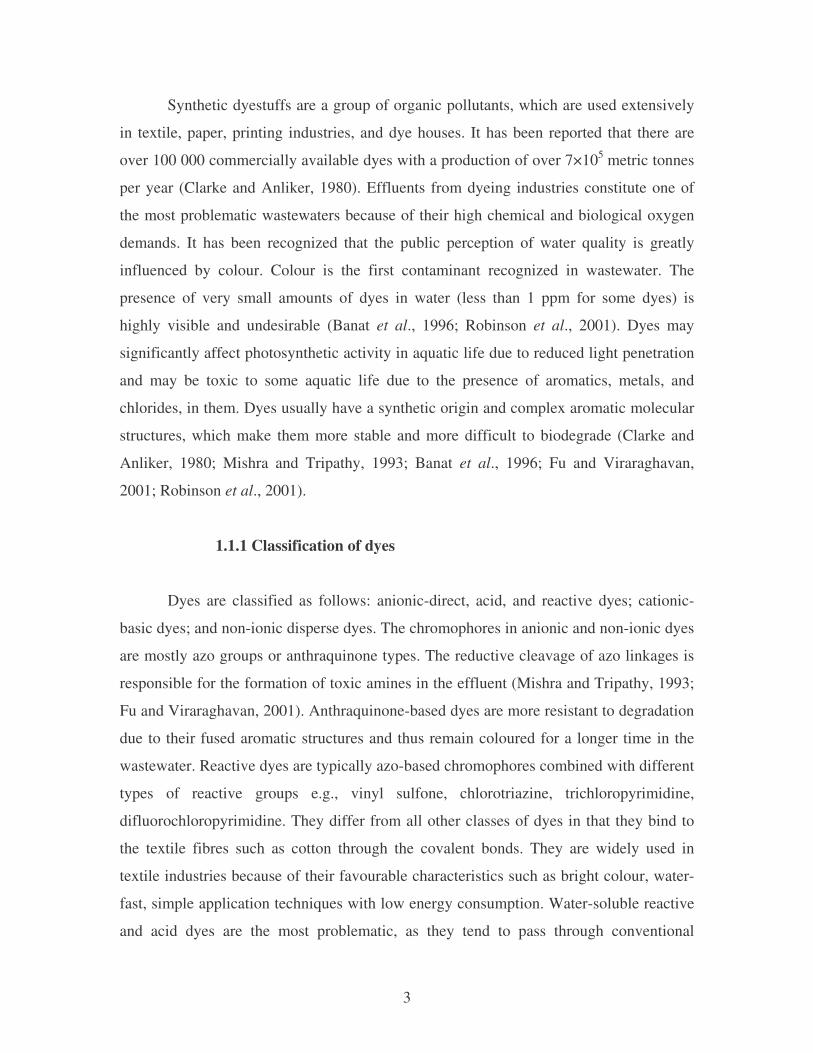
Synthetic dyestuffs are a group of organic pollutants, which are used extensively
in textile, paper, printing industries, and dye houses. It has been reported that there are
over 100 000 commercially available dyes with a production of over 7×10⁵ metric tonnes
per year (Clarke and Anliker, 1980). Effluents from dyeing industries constitute one of
the most problematic wastewaters because of their high chemical and biological oxygen
demands. It has been recognized that the public perception of water quality is greatly
influenced by colour. Colour is the first contaminant recognized in wastewater. The
presence of very small amounts of dyes in water (less than 1 ppm for some dyes) is
highly visible and undesirable (Banat et al., 1996; Robinson et al., 2001). Dyes may
significantly affect photosynthetic activity in aquatic life due to reduced light penetration
and may be toxic to some aquatic life due to the presence of aromatics, metals, and
chlorides, in them. Dyes usually have a synthetic origin and complex aromatic molecular
structures, which make them more stable and more difficult to biodegrade (Clarke and
Anliker, 1980; Mishra and Tripathy, 1993; Banat et al., 1996; Fu and Viraraghavan,
2001; Robinson et al., 2001).
1.1.1 Classification of dyes
Dyes are classified as follows: anionic-direct, acid, and reactive dyes; cationic-
basic dyes; and non-ionic disperse dyes. The chromophores in anionic and non-ionic dyes
are mostly azo groups or anthraquinone types. The reductive cleavage of azo linkages is
responsible for the formation of toxic amines in the effluent (Mishra and Tripathy, 1993;
Fu and Viraraghavan, 2001). Anthraquinone-based dyes are more resistant to degradation
due to their fused aromatic structures and thus remain coloured for a longer time in the
wastewater. Reactive dyes are typically azo-based chromophores combined with different
types of reactive groups e.g., vinyl sulfone, chlorotriazine, trichloropyrimidine,
difluorochloropyrimidine. They differ from all other classes of dyes in that they bind to
the textile fibres such as cotton through the covalent bonds. They are widely used in
textile industries because of their favourable characteristics such as bright colour, water-
fast, simple application techniques with low energy consumption. Water-soluble reactive
and acid dyes are the most problematic, as they tend to pass through conventional
4
treatment systems unaffected. Hence, their removal is also of great importance (Hu,
1992; Juang et al., 1997; Moran et al., 1997; Karcher et al., 1999; Aksu and Tezer, 2000;
Sumathi and Manju, 2000; Robinson et al., 2001; O’Mahony et al., 2002).
Basic dyes have high brilliance and intensity of colours and are highly visible
even in a very low concentration (Clarke and Anliker, 1980; Banat et al., 1996; Mittal
and Gupta, 1996; Fu and Viraraghavan, 2001; Chu and Chen, 2002; Fu and
Viraraghavan, 2002). Metal complex dyes are mostly based on chromium, which is
carcinogenic (Gupta et al., 1990; Mishra and Tripathy, 1993). Disperse dyes do not
ionize in an aqueous medium and some disperse dyes have also been shown to have a
tendency to bioaccumulate (Baughman and Perenich, 1988; Srivastava and Prakash,
1991). Due to the chemical stability and low biodegradability of these dyes, conventional
biological wastewater treatment systems are inefficient in treating dye wastewater.
Physical or chemical treatment processes are usually employed to treat dye wastewater.
These include chemical coagulation/flocculation, ozonation, oxidation, ion exchange,
irradiation, precipitation, and adsorption. Some of these techniques are effective, but have
their limitations. These include: excess amount of chemical usage, or accumulation of
concentrated sludge with obvious disposal problems; expensive plant requirements or
operational costs; lack of effective colour reduction; and sensitivity to a variable
wastewater input (McKay and Poots, 1980; El-Geundi, 1991; Juang et al., 1997; Lambert
et al., 1997; Low and Lee, 1997; Ramakrishna and Viraraghavan, 1997; Slokar and Le-
Marechal, 1997; Ho and McKay, 1999; Lee et al., 1999; Morais et al., 1999; Otero et al.,
2003).
In recent years, a number of studies have focused on some microorganisms, which
are able to biodegrade or bioaccumulate azo dyes in wastewaters (Dhodapkar et al.,
2006). A wide variety of microorganisms including bacteria, fungi, and algae are capable
of decolourizing a wide range of dyes via anaerobic, aerobic, and sequential anaerobic–
aerobic treatment processes. Cytoplasmic azo reductases play an important role in the
anaerobic biodegradation of azo dyes to produce colourless aromatic amines although
complete mineralization is difficult and the resulting aromatic amines may be toxic and

5
carcinogenic. These amines are resistant to further anaerobic mineralization. Fortunately,
once the xenobiotic azo component of the dye molecule has been removed, the resultant
amino compounds are good substrates for aerobic biodegradation suggesting a choice of a
sequential anaerobic–aerobic system for wastewater treatment (Razo-Flores et al., 1997;
Fu and Viraraghavan, 2001; Manu and Chaudhari, 2001). A number of aerobic biological
processes for the removal of dyes from textile effluents exist. This includes
decolourization through liquid fermentations by white-rot fungi (such as Phanerochaete
chrysosporium, Trametes versicolor, Coriolus versicolor); bacterial cultures (such as
Pseudomonas strains, mixed bacterial cultures, Bacillus subtilis) and yeasts (such as
Klyveromyces marxianus, Candida zeylanoides). Biochemical oxidation suffers from
significant limitations since more dyestuffs found in the commercial market have been
intentionally designed to be resistant to aerobic microbial degradation (Pearce et al.,
2003).
Reactive azo dyes are electron deficient in nature and this property makes them
less susceptible to oxidative catabolism (Banat et al., 1996). Research has shown that the
efficiency of biological treatment systems are greatly influenced by the operational
parameters, the composition of textile wastewater and the structure and substituents of
dye molecule. The level of aeration, temperature, pH, and redox potential of the system
are the variables that can be optimized to produce the maximum rate of dye reduction.
The ability of microorganisms to reduce dyes from wastewater depends on the classes of
dyes used (acidic, basic, direct, disperse, metal-complex, and reactive). The composition
of textile wastewater varies and can include organics, nutrients, salts, sulphur compounds
and toxicants as well as colour. Therefore, the inhibitory effect of any of these
compounds on the dye reduction process should be investigated (Glenn and Gold, 1983;
Knapp and Newby, 1999; Kapdan et al., 2000; Meehan et al., 2000; Fu and
Viraraghavan, 2001; Manu and Chaudhari, 2001; Ramalho et al., 2002). Another
biological treatment method is bioaccumulation. Bioaccumulation is defined as the
accumulation of pollutants by actively growing cells by metabolism; temperature-
independent; and metabolism-dependent mechanism steps. Although bioaccumulations of
dyes by yeasts were accomplished, significant practical limitations exist. These include
6
the inhibition of cell growth at high dye concentrations and requirement of metabolic
energy externally provided (Dönmez, 2002; Aksu, 2003). Therefore, there is a need to
find alternative treatment methods that are effective in removing dyes from large volumes
of effluents and are low in cost, such as biosorption or bioflocculation.
1.2 THE NEED FOR WASTEWATER TREATMENT
Matter in water may be broadly classified according to its origin as inorganic
mineral matter or organic carbonaceous material. Substances producing turbidity are
often inorganic, while those causing taste, odour, and colour are generally organic
compounds. The particles producing turbidity may be further classified according to their
size, which may range from molecular dimensions of 50 microns or larger. The fraction
greater than 1 micron in diameter is generally referred to as silt and will settle out on
standing. The smaller particles, which are classified as colloidal, will remain suspended
for very long time. Most attention has therefore been directed towards the use of
coagulation for removal of colloidal material, although this process also removes the
larger particles (Jones, 1998). It is important to keep our water clean because of our
environment and health. Some of the reasons include:
• Fisheries; clean water is critical to plants and animals that live in water. This is
important to the fishing industry, sport fishing enthusiasts, and future generations;
• Wildlife habitat, rivers and ocean waters teem with life that depends on shoreline,
beaches, and marshes. They are critical habitats for hundreds of species of fish
and other aquatic life. Migratory water birds use the areas for resting and feeding;
• Recreation and quality of life; water is a great playground for us all. The scenic
and recreational values of our waters are reasons many people choose to live
where they do. Visitors are drawn to water activities such as swimming, fishing,
boating, and picnicking; and
• Health concern; water may carry disease if not properly cleaned. Since we live,
work and play so close to water, harmful bacteria have to be removed to make
water safe (Cowan and Talaro, 2006).
7
1.3 WATER SOURCES AND QUALITY
Water is usually withdrawn for drinking and household purposes from the
following sources (Navin et al., 2006):
• Ground water (springs, infiltration galleries, and wells)
• Surface water (rivers, lakes, ponds, streams, impounded reservoirs, and stored
rainwater).
Ground water is one of the nation’s most important natural resources. Ground
water provides drinking water for more than one-half of the nation’s population and is the
sole source of drinking water for many rural communities and some large cities. In 1990,
ground water accounted for 39% of the public water supply for cities and towns and 96%
for self-supplied systems for domestic use (Twarakavi and Kaluarachchi, 2006). It is also
the source of much of the water used for irrigation. Ground water is a major contributor
to flow in many streams and rivers and has a strong influence on river and wetland
habitats for plants and animals. Ground water withdrawal in the USA in 1995 was
estimated to be approximately 77 billion gallons per day, which is about 8% of the
estimated 1 trillion gallons per day of natural recharge to the ground water system of the
USA (Navin et al., 2006; Twarakavi and Kaluarachchi, 2006).
If groundwater is conveniently located and in sufficient quantities it should be
used, as it is less polluted compared with surface water. Groundwater may be aerobic or
anaerobic depending on the environmental conditions where it is located. The anaerobic
groundwater often contains CO2, which makes it corrosive. The removal of CO2 as well
as provision of oxygen can be facilitated by aeration. Chlorination also removes CO2.
Some ground water contains excessive amounts of Fe, Mn, hardness, and/or fluoride
(Decker and Long, 1992).
The surface waters are generally more polluted than groundwater due to their
exposure to the environment. They may require more treatment steps than ground water.
8
The typical impurities may include turbidity, colour, algae, floating debris, bacteria, and
other microorganisms, in addition to the constituents of ground water. Surface water in
general contains physical, chemical, and biological impurities (such as clay, sand,
colloids, minerals, colour, odour, taste, and microorganisms). Rivers have been used by
man since the dawn of civilization as a source of water, for food, for transport, as a
source of power to drive machinery, and a means of disposing of waste (Vigneswaran
and Visvanathan, 1995).Thus river water requires adequate treatment steps so that it can
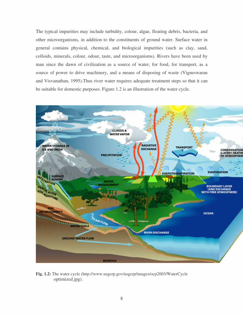
be suitable for domestic purposes. Figure 1.2 is an illustration of the water cycle.
Fig. 1.2: The water cycle (http://www.usgcrp.gov/usgcrp/images/ocp2003/WaterCycle optimized.jpg).
9
The majority of water supplies require treatment to make them suitable for use in
domestic and industrial applications. Although appearance, taste, and odour are useful
indicators of the quality of drinking water, suitability in terms of public is determined by
microbiological, physical, chemical, and radiological characteristics. Of these, the most
important is microbiological quality. In addition, a number of chemical contaminants
(both organic and inorganic) are found in water. These may lead to health problems.
Therefore, detailed analyses of water are warranted (Vigneswaran and Visvanathan,
1995). The drinking water thus should be; free from pathogenic (disease causing)
organisms; clear (i.e., low turbidity, little colour); not saline (salty); free from offensive
taste or smell; and free from compounds that may have adverse effects on human health
(harmful in the long term) (Vigneswaran and Visvanathan, 1995).
1.4 WASTEWATER TREATMENT PROCESSES
The major aim of wastewater treatment is to remove as much of the suspended
solids as possible before the remaining water, called effluent, is discharged back to the
environment. As solid material decays, it uses up oxygen, which is needed by the plants
and animals living in the water. Conventional wastewater treatment process involves
primary, secondary, and tertiary treatment (Prescott et al., 1996; Nester et al., 2001).
1.4.1 Primary treatment
Primary treatment involves aerating (stirring up) the wastewater, in order to
replenish oxygen back in. Primary treatment can remove 20 to 30% of the BOD, which is
present in particulate form and about 60% of suspended solids from wastewater. In this
treatment, particulate material is removed by screening, precipitation of small particles,
and settling in basins or tanks. The resulting solid material is called sludge. This
treatment of physical removal of settleable solids (primary treatment) and secondary
treatment (biological transformation of dissolved organic matter to microbial biomass and
carbon dioxide) is shown together with final clarifiers. The final clarifiers separate the
10
newly formed microbial biomass (sewage sludge) from the processed water stream,
which can be returned to the receiving body of water (Prescott et al., 1996).
1.4.2 Secondary treatment
Secondary treatment is used after primary treatment for the biological removal of
dissolved organic matter. This process removes about 90 to 95% of the BOD and many
bacterial pathogens and more than 90% of suspended solids. Several approaches
involving similar microbial activities can be used for secondary treatment to biologically
remove dissolved organic matter. Under aerobic conditions, dissolved organic matter is
transformed into additional microbial biomass plus carbon dioxide (Ford, 1993). When
these processes occur with lower oxygen levels or with a microbial community too young
or too old, unsatisfactory floc formation and settling can occur. The result is a bulking
sludge, caused by massive development of filamentous bacteria such as Sphaerotilus and
thiothrix, together with many poorly characterized filamentous organisms. These
important filamentous bacteria form flocs that do not settle well and have effluent quality
problems (Prescott et al., 1996).
An aerobic activated sludge process is a biological method of wastewater
treatment that is performed by a variable and mixed community of microorganisms in an
aerobic aquatic environment. These microorganisms derive energy from carbonaceous
organic matter in aerated wastewater for the production of new cells in a process known
as synthesis. Simultaneously energy is released through the conversion of this organic
matter into compounds that contain lower energy, such as carbon dioxide and water, in a
process called respiration. A variable number of microorganisms in the system obtain
energy by converting ammonia nitrogen to nitrate nitrogen in a process termed
nitrification. In this consortium of microorganisms, the biological component of the
process is known collectively as activated sludge. The overall goal of the activated-
sludge process is to remove substances that have a demand for oxygen from the system
(Huang and Shui, 1996).
11
After the bacteria and fungi in sewage treatment have used certain nutrients, they
serve as food for ciliates, protozoa, nematodes, and other forms of life. The end result is a
small increase in the mass of organisms present in a given amount of treated sewage and
a large decrease in the amount of biodegradable organic material (Bitton, 1994). The
increased microbial biomass in the sewage is removed to the digester; a portion is left
behind as inoculum to act on a new load of waste material. Within the sewage digester,
anaerobic organisms act on the solids remaining in sewage after its aerobic treatment.
The digester provides anaerobic conversion of organic to inorganic matter and removes
water from the sewage so that a minimum of solid matter remains in it. Various
populations act sequentially. In the sewage digester, the anaerobic methane-forming
organisms can perform their role of converting the simple organic acids in sewage into
the useful end product methane (CH4). Many sewage treatment plants are equipped to use
their own methane, thereby avoiding the cost of other sources of energy to run their
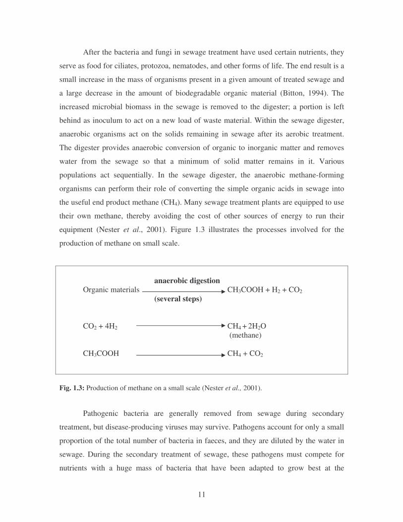
equipment (Nester et al., 2001). Figure 1.3 illustrates the processes involved for the
production of methane on small scale.
anaerobic digestion Organic materials CH3COOH + H2 + CO2 (several steps)
CO2 + 4H2 CH4 + 2H2O (methane)
CH3COOH CH4 + CO2
Fig. 1.3: Production of methane on a small scale (Nester et al., 2001).
Pathogenic bacteria are generally removed from sewage during secondary
treatment, but disease-producing viruses may survive. Pathogens account for only a small
proportion of the total number of bacteria in faeces, and they are diluted by the water in
sewage. During the secondary treatment of sewage, these pathogens must compete for
nutrients with a huge mass of bacteria that have been adapted to grow best at the
12
temperature and conditions provided. As a result, most pathogenic bacteria are
overgrown and are eliminated by their competitors (Huang and Shui, 1996). Animal
viruses lack appropriate host cells in sewage and replicate there, although they may
survive for long periods. If large quantities of virus particles are present in raw sewage,
some may be recovered after secondary treatment. Although sewage effluents are often
chlorinated before being discharged into receiving waters, chlorine treatment at this stage
does not inactivate viruses. The virus particles are commonly enclosed within small
clumps of effluent materials where they are protected from the chlorine. Because viruses
do adhere to large particles, they can be removed along with other solid materials (Huang
and Shui, 1996; Nester et al., 2001).
1.4.3 Tertiary treatment
Tertiary treatment purifies wastewater more than is possible with primary and
secondary treatments. The goal is to remove such pollutants as nonbiodegradable organic
matter e.g. polychlorinated biphenyls, heavy metals, and minerals (Prescott et al., 1996).
Tertiary treatment provides a final stage to raise the effluent quality to the standard
required before it is discharged to the receiving environment (sea, river, lake, and
ground). The large quantities of phosphates or nitrites remaining in sewage after
secondary treatment may increase the growth of microorganism, which gradually deplete
the oxygen and thus threaten other forms of aquatic life. The tertiary treatment of sewage,
to remove nitrates and phosphates, can greatly alleviate this problem (Cowan et al.,
1995).
In some designs for the tertiary treatment of sewage, chemical precipitation of
phosphates has been combined with biological removal of nitrates. Certain bacteria
(particularly species of Pseudomonas and Bacillus) can completely reduce nitrates (NO3-)
to N2 (denitrification). The N2 gas is inert, non-toxic, and easily removed. More than one
tertiary treatment process may be used at any treatment plant. If disinfection is practiced,
it is always the final process. It is also called "effluent polishing” (Nester et al., 2001).
Figure 1.4 is an illustration of the major steps in modern sewage treatment plant.

13
Fig. 1.4: Major steps involved in modern sewage treatment plants (http://web.deu.edu.tr/atiksu/toprak/summary4.html).
1.5 TECHNOLOGIES AVAILABLE FOR COLOUR REMOVAL FROM
EFFLUENTS
There are several reported technologies for the removal of dyes from effluents
(Table 1.1). The technologies can be divided into three categories: biological, chemical
and physical (Robinson et al., 2001). Many of these conventional methods for treating
dye wastewater have not been widely applied on a large scale in the textile and paper
industries because of the high cost and disposal problems (Ghoreishi and Haghighi,
2003). At the present time, there is no single process capable of adequate treatment,
mainly due to the complex nature of the effluents (Marco et al., 1997; Pereira et al.,
2003). In practice, a combination of different processes is often used to achieve the
desired water quality in the most economical way. Research is ongoing and in the areas
14
of combined adsorption-biological treatments in order to improve the biodegradation of
dyestuffs and minimize the sludge production (Pearce et al., 2003).
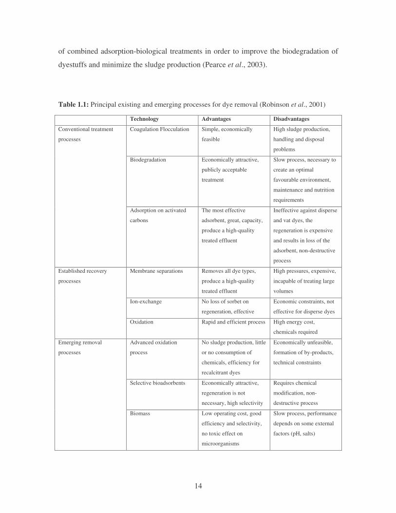
Table 1.1: Principal existing and emerging processes for dye removal (Robinson et al., 2001) Technology Advantages Disadvantages
Coagulation Flocculation Simple, economically
feasible
High sludge production,
handling and disposal
problems
Biodegradation Economically attractive,
publicly acceptable
treatment
Slow process, necessary to
create an optimal
favourable environment,
maintenance and nutrition
requirements
Conventional treatment
processes
Adsorption on activated
carbons
The most effective
adsorbent, great, capacity,
produce a high-quality
treated effluent
Ineffective against disperse
and vat dyes, the
regeneration is expensive
and results in loss of the
adsorbent, non-destructive
process
Membrane separations Removes all dye types,
produce a high-quality
treated effluent
High pressures, expensive,
incapable of treating large
volumes
Ion-exchange No loss of sorbet on
regeneration, effective
Economic constraints, not
effective for disperse dyes
Established recovery
processes
Oxidation Rapid and efficient process High energy cost,
chemicals required
Advanced oxidation
process
No sludge production, little
or no consumption of
chemicals, efficiency for
recalcitrant dyes
Economically unfeasible,
formation of by-products,
technical constraints
Selective bioadsorbents Economically attractive,
regeneration is not
necessary, high selectivity
Requires chemical
modification, non-
destructive process
Emerging removal
processes
Biomass Low operating cost, good
efficiency and selectivity,
no toxic effect on
microorganisms
Slow process, performance
depends on some external
factors (pH, salts)
15
1.5.1 Biological treatments
Biological treatment is often the most economical alternative compared to
physical and chemical processes. Biodegradation methods such as fungal decolourization,
microbial degradation, adsorption by (living or dead) microbial biomass and
bioremediation systems are commonly applied to the treatment of industrial effluents
because many microorganisms such as bacteria, yeasts, algae and fungi are able to
accumulate and degrade different pollutants (Fu and Viraraghavan, 2001; McMullan et
al., 2001). However, their application is often restricted because of technical constraints.
Biological treatment requires a large land area and is constrained by sensitivity toward
diurnal variation as well as toxicity of some chemicals, and less flexibility in design and
operation (Bhattacharyya and Sarma, 2003). Biological treatment is incapable of
obtaining satisfactory colour elimination with current conventional biodegradation
processes (Robinson et al., 2001). Moreover, although many organic molecules are
degraded, many others are recalcitrant due to their complex chemical structure and
synthetic organic origin. In particular, due to their xenobiotic nature, azo dyes are not
totally degraded (Ravi-Kumar et al., 1998).
1.5.2 Chemical treatments
Chemical methods include coagulation or flocculation combined with flotation
and filtration, precipitation–flocculation with Fe(II)/Ca(OH)2, electroflotation,
electrokinetic coagulation, conventional oxidation methods by oxidizing agents (ozone),
irradiation or electrochemical processes. These chemical techniques are often expensive,
and although the dyes are removed, accumulation of concentrated sludge creates a
disposal problem. There is also the possibility that a secondary pollution problem may
arise because of excessive chemical use. Recently, other emerging techniques, known as
advanced oxidation processes, which are based on the generation of very powerful
oxidizing agents such as hydroxyl radicals, have been applied with success for pollutant
degradation. Although these methods are efficient for the treatment of waters
contaminated with pollutants, they are costly and commercially unattractive. The high
16
electrical energy demand and the consumption of chemical reagents are common
problems (Crini, 2006).
1.5.3 Physical treatments
Different physical methods are also widely used, such as membrane-filtration
processes (nanofiltration, reverse osmosis, electrodialysis) and adsorption techniques.
The major disadvantage of the membrane processes is that they have a limited lifetime
before membrane fouling occurs. The cost of periodic membrane replacement must thus
be included in any analysis for their economic viability. In accordance with the literature,
liquid-phase adsorption is one of the most popular methods for the removal of pollutants
from wastewater. Proper design of the adsorption process may produce a high-quality
treated effluent. This process provides an attractive alternative for the treatment of
contaminated waters, especially if the sorbent is inexpensive and does not require an
additional pre-treatment step before its application (Dabrowski, 2001).
Adsorption is a well known equilibrium separation process and an effective
method for water decontamination applications. Adsorption has been found to be superior
to other techniques for water re-use in terms of initial cost, flexibility and simplicity of
design, ease of operation and insensitivity to toxic pollutants. Adsorption also does not
result in the formation of harmful substances (Dabrowski, 2001).
1.6 MECHANISM OF COLOUR REMOVAL BY BACTERIA
The simplest mechanism of colour removal by whole bacterial cells is that of the
adsorption of the dye onto the biomass (Bras et al., 2001). However, this mechanism is
similar to many other physical adsorption mechanisms for the removal of colour. It is not
suitable for long-term treatment and during adsorption; the dye is concentrated onto the
biomass, which will become saturated with time. The dye-adsorbent composition must
also be disposed off. Bio-association between the dye and the bacterial cells tends to be
17
the first step in the biological reduction of azo dyes, which is a destructive treatment
technology (Southern, 1995).
Biodegradation processes may be anaerobic, aerobic or involve a combination of
both. In the reaction between bacterial cells and azo dyes, there are significant differences
between the physiology of microorganisms grown under aerobic and anaerobic
conditions. For aerobic bacteria to be significant in the reductive process, the bacteria
must be specifically adapted. This adaptation involves long-term aerobic growth in
continuous culture in the presence of a very simple azo compound. The bacteria
synthesise an azoreductase specific for this compound, which, under controlled
conditions, can reductively cleave the azo group in the presence of oxygen. In contrast,
bacterial reduction under anaerobic conditions is relatively unspecific with regard to the
azo compounds involved, and is, therefore, of more use for the removal of colour in azo
dye wastewater (Stolz, 2001).
It is thought that, as most azo dyes have sulphonate substituent groups and a high
molecular weight, they are unlikely to pass through cell membranes. Therefore, the
reducing activity referred to above is not dependant on the intracellular uptake of the dye
(Robinson et al., 2002). This was shown by Russ et al. (2000), who also suggested that
bacterial membranes are almost impermeable to flavin-containing cofactors and,
therefore, restrict the transfer of reduction equivalents by flavins from the cytoplasm to
the sulphonated azo dyes. Thus, a mechanism other than reduction by reduced flavins
formed by cytoplasmic flavin-dependent azoreductases might be responsible for
sulphonated azo dye reduction in bacterial cells with intact cell membranes (Russ et al.,
2000).
One such mechanism involves the electron transport-linked reduction of azo dyes
in the extra-cellular environment. To achieve this, bacteria must establish a link between
their intracellular electron transport systems and the high molecular weight, azo dye
molecules. For such a link to be established, the electron transport components must be
localised in the outer membrane of the bacterial cells (in the case of gram-negative
18
bacteria), where they can make direct contact with either the azo dye substrate or a redox
mediator at the cell surface (Myers and Myers, 1992). In addition, low molecular weight
redox mediator compounds can act as electron shuttles between the azo dye and an
NADH (nicotinamide adenine dinucleotide)-dependent azo reductase that is situated in
the outer membrane. These mediator compounds are either formed during the metabolism
of certain substrates by the bacteria or they may be added externally (Gingell and Walker,
1971).
The addition of synthetic redox mediators such as anthraquinone sulphonates,
even at very low concentrations, will facilitate the non-enzymatic reduction of the azo
dyes in the extra-cellular environment (Plumb et al., 2001; Yoo et al., 2001). However, if
the extra-cellular environment is aerobic, this reduction mechanism would be inhibited by
oxygen, due to the preferential oxidation of the reduced redox mediator by oxygen rather
than by the azo dye. Membrane-bound azo reductase activity, mediated by redox
compounds, is different from the soluble cytoplasmic azo reductase that is responsible for
the reduction of non-sulphonated dyes that permeate through the cell membrane. Their
results show that a thiol-specific inhibitor almost completely inactivates the membrane-
bound azo reductase in Sphingomonas sp. but had no effect on the cytoplasmic azo
reductase. Therefore, the membrane-bound and the cytoplasmic azo reductases are two
different enzyme systems (Kudlich et al., 1997).
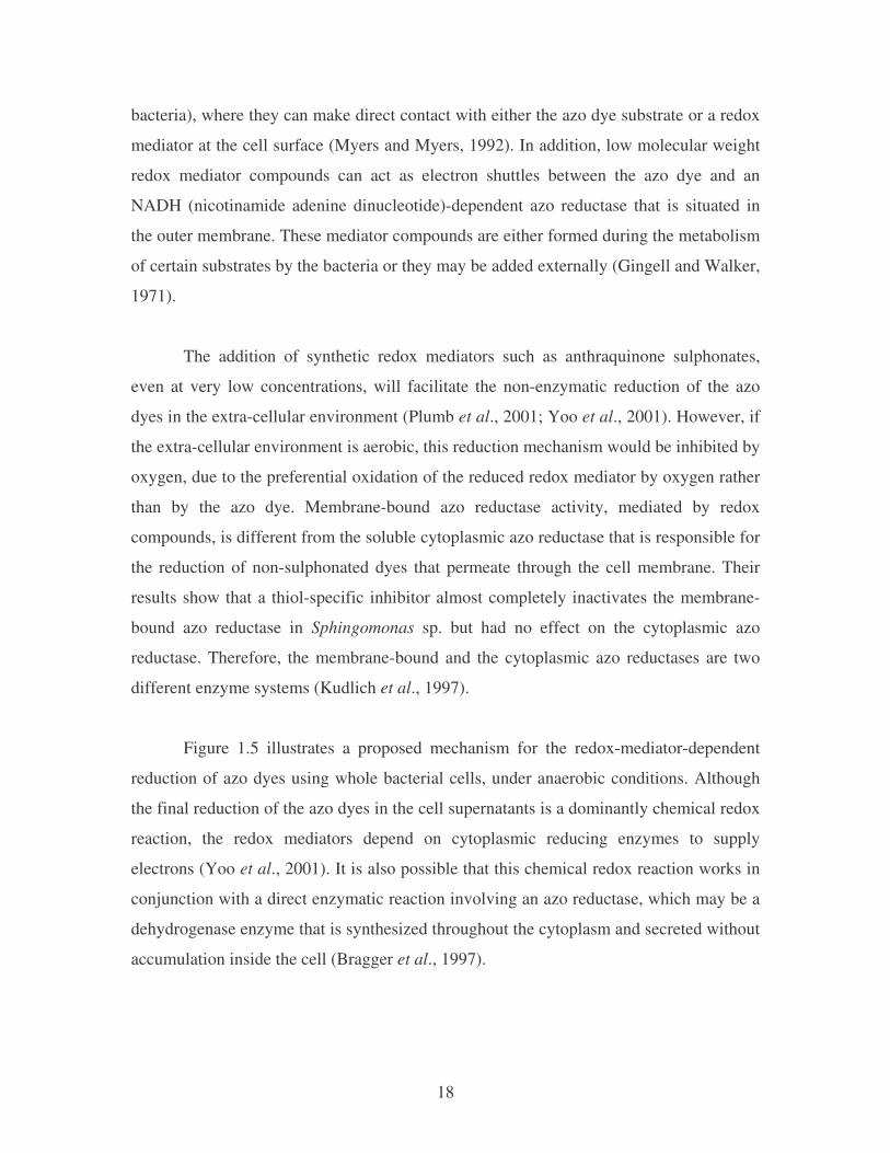
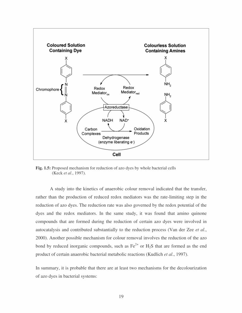
Figure 1.5 illustrates a proposed mechanism for the redox-mediator-dependent
reduction of azo dyes using whole bacterial cells, under anaerobic conditions. Although
the final reduction of the azo dyes in the cell supernatants is a dominantly chemical redox
reaction, the redox mediators depend on cytoplasmic reducing enzymes to supply
electrons (Yoo et al., 2001). It is also possible that this chemical redox reaction works in
conjunction with a direct enzymatic reaction involving an azo reductase, which may be a
dehydrogenase enzyme that is synthesized throughout the cytoplasm and secreted without
accumulation inside the cell (Bragger et al., 1997).
19
Fig. 1.5: Proposed mechanism for reduction of azo dyes by whole bacterial cells (Keck et al., 1997).
A study into the kinetics of anaerobic colour removal indicated that the transfer,
rather than the production of reduced redox mediators was the rate-limiting step in the
reduction of azo dyes. The reduction rate was also governed by the redox potential of the
dyes and the redox mediators. In the same study, it was found that amino quinone
compounds that are formed during the reduction of certain azo dyes were involved in
autocatalysis and contributed substantially to the reduction process (Van der Zee et al.,
2000). Another possible mechanism for colour removal involves the reduction of the azo
bond by reduced inorganic compounds, such as Fe2+ or H2S that are formed as the end
product of certain anaerobic bacterial metabolic reactions (Kudlich et al., 1997).
In summary, it is probable that there are at least two mechanisms for the decolourization
of azo dyes in bacterial systems:
20
• Direct electron transfer to azo dyes as terminal electron acceptors via enzymes
during bacterial catabolism, connected to ATP-generation (energy conservation);
and
• Reduction of azo dyes by the end products of bacterial catabolism not linked to
ATP-generation.
Organics or inorganics may be involved in both mechanisms by acting as electron
shuttles between the reducing equivalents and the azo dyes (Yoo et al., 2000).
1.6.1 Colour removal using whole bacterial cells
Alternative approaches to colour removal, utilizing microbial biocatalysts to
reduce the dyes that are present in the effluent, offer potential advantages over physio-
chemical processes. In particular, the ability of whole bacterial cells to metabolise azo
dyes has been extensively investigated (Pearce et al., 2003). Under aerobic conditions,
azo dyes are not readily metabolized (Robinson et al., 2001). However, under anaerobic
conditions, many bacteria reduce the highly electrophilic azo bond in the dye molecule,
reportedly by the activity of low specificity cytoplasmic azo reductases, to produce
colourless aromatic amines. These amines are resistant to further anaerobic
mineralization and can be toxic or mutagenic to animals. Fortunately, once the xenobiotic
azo component of the dye molecule has been removed, the resultant amino compounds
are good substrates for aerobic biodegradation. According to Lourenco et al. (2000), if a
sequential anaerobic–aerobic system is employed for wastewater treatment, the amines
can be mineralised under aerobic conditions by a hydroxylation pathway involving a ring
opening mechanism. Degradation of dyes in coloured wastewater involves the use of
whole cells rather than isolated enzymes. This approach is advantageous because of the
high costs associated with enzyme purification. In addition, degradation is often
associated with a number of enzymes working sequentially (Pearce et al., 2003).
21
1.6.2 Colour removal using mixed bacterial cultures
Degradation of xenobiotics such as azo dyes is often carried out by mixed cultures
(Knackmuss, 1996; Pearce et al., 2003). Pearce et al. (2003) have reported that a higher
degree of biodegradation and mineralization can be expected when co-metabolic
activities within a microbial community complement each other. Knackmuss (1996)
gives an example of this using the degradation of naphthalene sulphonates by a two-
species culture. Sphingomonas strain BN6 was able to degrade naphthalene-2-sulphonate,
a building block of azo dyes, into salicylate ion equivalents. The salicylate ion cannot be
further degraded and is toxic to strain BN6. Therefore, naphthalene-2-sulphonate can
only be degraded completely in the presence of a complementary organism that is
capable of degrading the salicylate ion (Knackmuss, 1996). In addition, it can be difficult
to isolate a single bacterial strain from dye-containing wastewater samples and, in some
instances, long term adaptation procedures are necessary before the isolate is capable of
using the azo dye as a respiratory substrate (Pearce et al., 2003).
.
1.6.3 Colour removal using single bacterial cultures
The advantages of mixed cultures are apparent as some microbial consortia can
collectively carry out biodegradation tasks that no individual pure strain can undertake
successfully (Nigam et al., 1996). In addition, mixed culture studies may be more
comparable to practical situations. However, mixed cultures only provide an average
macroscopic view of what is happening in the system and results are not easily
reproduced, making thorough, effective interpretation difficult. For these reasons, a
substantial amount of research on the subject of colour removal has been employed using
single bacterial cultures. The use of a pure culture system ensures that the data are
reproducible and that the interpretation of experimental observations is easier (Chang and
Lin, 2000).
22
1.7 NOVEL AND ESTABLISHED APPLICATIONS OF MICROBIAL
POLYSACCHARIDES
Flocculation in microbial systems was first reported by Louis Pasteur 1876 (cited
by Salehizadeh and Shojaosadati, 2001) for the yeast Levure casseeuse. Two years later,
this phenomenon was observed in bacterial cultures (Salehizadeh and Shojaosadati,
2001). Butterfield (1935) isolated Zoogloea-forming bacteria from activated sludge in
1935. Later, bioflocculation was investigated extensively and a correlation was
established between the accumulation of extracellular biopolymeric flocculants (EBFs)
and cell aggregation (McKinney, 1956; Tenny and Stumm 1965). Many EBF-producing
microorganisms including bacteria, fungi, yeast, and algae have since been isolated from
soil and wastewater (Bar-or and Shilo, 1987; Bender et al., 1989; Huang, 1990; Kakii et
al., 1990; Morgan et al., 1990; Fumio, 1991; Hantula and Bamford, 1991a, b; Dube,
1992; Guirand, 1992; Sousa et al., 1992; Kim, 1993; Seo, 1993; Kurane et al., 1995;
Yokoi et al., 1995; Suh et al., 1997; Salehizadeh et al ., 1998; Tong et al., 1999; Misra,
2002).
Many microorganisms synthesize exopolysaccharides (EPS) or EBFs, which
either remain attached to the cell surface or are found in the extracellular medium in the
form of amorphous slime. In the natural environments in which the microorganisms are
found, such polymers may either be associated with virulence, as in the case of plant or
animal pathogens, with plant microbial interactions or even protect the microbial cell
against desiccation or attack by bacteriophages and protozoa. In both natural and man-
made environments, the EPS play a major structural role in ‘biofilms’, the normal habitat
of many microbial communities, in which varying numbers of prokaryotic and eukaryotic
microorganisms grow while attached to solid-liquid interfaces (Yokoi et al., 1995;
Salehizadeh et al., 1998). Several such microbial polysaccharides are now widely
accepted products of biotechnology, while others are in various stages of development.
The uses of such polymers vary widely; some are employed because of their unique or
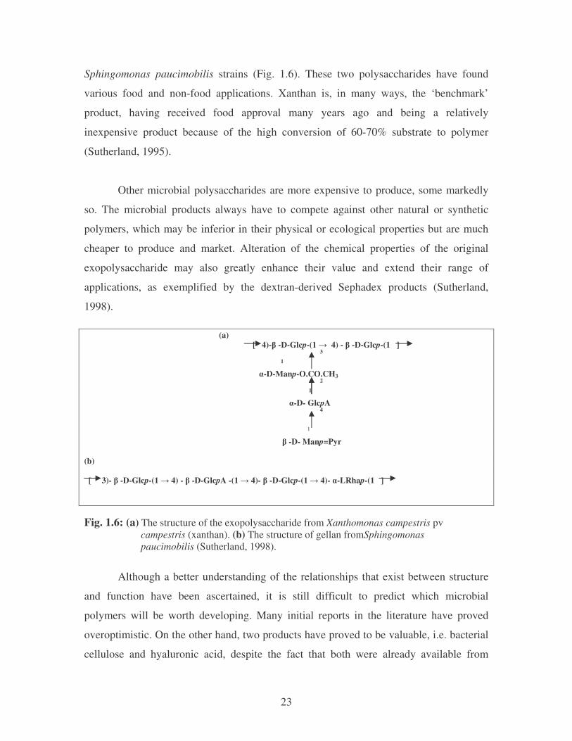
superior physical properties relative to traditional plant polysaccharides. In this category
are xanthans, from Xanthomonas campestris pv. campestris and gellan (Gelrite) from
23
Sphingomonas paucimobilis strains (Fig. 1.6). These two polysaccharides have found
various food and non-food applications. Xanthan is, in many ways, the ‘benchmark’
product, having received food approval many years ago and being a relatively
inexpensive product because of the high conversion of 60-70% substrate to polymer
(Sutherland, 1995).
Other microbial polysaccharides are more expensive to produce, some markedly
so. The microbial products always have to compete against other natural or synthetic
polymers, which may be inferior in their physical or ecological properties but are much
cheaper to produce and market. Alteration of the chemical properties of the original
exopolysaccharide may also greatly enhance their value and extend their range of
applications, as exemplified by the dextran-derived Sephadex products (Sutherland,
1998).
(a) [ 4)-� -D-Glcp-(1 � 4) - � -D-Glcp-(1 ] 3
1
�-D-Manp-O.CO.CH3 2
1
�-D- GlcpA
4
1
� -D- Manp=Pyr (b) [ 3)- � -D-Glcp-(1 � 4) - � -D-GlcpA -(1 � 4)- � -D-Glcp-(1 � 4)- �-LRhap-(1 ] Fig. 1.6: (a) The structure of the exopolysaccharide from Xanthomonas campestris pv campestris (xanthan). (b) The structure of gellan fromSphingomonas paucimobilis (Sutherland, 1998).
Although a better understanding of the relationships that exist between structure
and function have been ascertained, it is still difficult to predict which microbial
polymers will be worth developing. Many initial reports in the literature have proved
overoptimistic. On the other hand, two products have proved to be valuable, i.e. bacterial
cellulose and hyaluronic acid, despite the fact that both were already available from
24
nonbacterial sources. Another example of biological properties that have led to a
polysaccharide application can be found in the range of fungal 1.4-�-D-glucans, which
have proved to be potent immune-system modulators, a property that is still poorly
understood (Sutherland, 1990).
1.7.1 �-D Glucan
1.7.1.1 Bacterial cellulose
Two groups of �-D-glucans are of biotechnological interest. Bacterial cellulose is
perhaps the more surprising, given the universal availability and cheapness, of plant
cellulose. In contrast to its role in the wall of plants, cellulose is produced as an
exopolysaccharide by Acetobacter xylinum and others, mainly Gram-negative bacterial
species. It is excreted into the medium where it rapidly aggregates as microfibrils,
yielding a surface pellicle. Fermenter design and the degree of aeration are important
factors in optimizing yield. Bacterial cellulose is essentially a high-value speciality
chemical with specific applications and usage. Some are produced commercially as a
source of highly pure polymer in the so-called cellulose-I form (60% I�: 40% I�), free
from lignin and other noncellulosic material. The fibrils form a unique ribbon 3-8 nm
thick and approximately 100 nm wide, which differ in morphology from other native
celluloses (Fig. 1.6). Bacterial cellulose also forms the basis for high-quality acoustic-
diaphragm membranes, in which the distribution of the fibrils containing a parallel
orientation of the glucan chains yield fibres possessing high tensile strengths. Bacterial
cellulose can also be used as a binder for ceramic powders and minerals and as a
thickener for adhesives (Yoshinaga et al., 1997).
1.7.1.2 (1 � 3) �-D- glucans from bacteria and fungi
Several bacteria, including Agrobacterium and Rhizobium species, can
each produce several EPS under appropriate physiological conditions. One of these is
curdlan, a neutral gel forming 1.3-� -D-glucan of relatively low molecular weight

25
(approximately 74 000 g/mol). Curdlan is formed in the stationary phase following
depletion of nitrogen and is insoluble in cold water but can be dissolved in hot water or in
dimethylsulphoxide. Curdlan forms a weak gel on heating above 55°C followed by
cooling. Further heating to 80-100°C increases the gel strength and produces a firm,
resilient gel, while autoclaving at 120°C converts the molecular structure to a triple helix.
The gel formed by this high-temperature treatment no longer melts when heated and,
unlike the similar alginate gels, is independent of the presence of divalent cations. The
gels are intermediate in properties between the high elasticity of gelatine and the
brittleness of agar. Those formed at higher temperature do not melt below 140°C. They
are very susceptible to shrinkage and syneresis but resistant to degradation by most �-D-
glucanases (Vossoughl and Buller, 1991).
1.7.2 Pullulan
Aureobasidium pullulans synthesizes a �-D-glucan in which maltotriose and a
small number of maltotetraose units (1.4- � -linked) are coupled through 1.6 � –bonds to
form an essentially linear polymer. The molecular mass is between 103 and 3 x 10⁶ and is
dependent on the physiological conditions and the culture strain used (Wiley et al., 1993).
Pullulan is not degraded by most amylases, but specific pullulanase enzymes (isolated
from sources including Enterobacter aerogenes) can be used to hydrolyze the
polysaccharide to its component maltotriose (and maltotetraose) units and thus provide a
useful means of preparing these oligosaccharides. Similar products are formed by several
other fungal species including Tremella mesenterica and Cyttaria harioti. Pullulan is
highly water soluble, forming viscous solutions that are stable in the presence of most
cations, but does not form gels. Esterification can be used both to increase its range of
physical properties and to reduce its susceptibility to enzyme attack. A proposed use of
pullulan is to form oil-resistant, water-soluble films with low oxygen permeability. This
novel packaging material assists in flavour retention and maintains the fresh appearance
of foods, which can then be cooked directly. Solutions of the polymer can also be used to
form odourless and tasteless coating directly onto food. These applications have
26
apparently been made in Japan, but usage of the polymer in other countries appears to be
limited (Nguyen et al., 1988).
1.7.3 Gellan and related polysaccharides
In its native form gellan carries O-acetyl and glyceryl substituents on a linear
polymer of 500 kDa that is composed of tetrasaccharide repeat units (Fig. 1.6). The acyl
groups inhibit crystallization of localized regions of the gellan chains and weak elastic
thermoreversible gels are formed. Deacylation causes extensive intermolecular
association, and strong, brittle gels form with various cations. Control of the degree of
acylation of the polymer yields a range of gel textures with properties similar in some
respects to agar, alginate or carrageenan gels. Gellan forms thermoreversible gels and
concentrations as low as 0.75% provides high gel strength. Marketed as Kelcogelm or
Gelrite, gellan has approval in the USA and the EU for food use as a gelling, stabilizing,
and suspending agent for a wide range of foods, either on its own or in combination with
other hydrocolloids. The gels give good flavour release and are stable over the wide pH
range found in food products. As a replacement for agar, Gelrite can be incorporated into
microbiological and cell-culture media. It may even lead to some growth enhancement
when compared with agar-based bacterial culture media. The high clarity of the gels may
have distinct advantages, as may the lower concentration required to provide gels of
equivalent strength (Pollock, 1993).
1.7.4 Xanthan
Xanthan, from Xanthomonas campestris, is a major commercial biopolymer.
Production from several commercial sources probably exceeds 20 000 tonnes per annum.
Alternate glucose residues of a cellulose backbone carry the side-chains composed of D-
mannose and D-glucuronic acid (Fig. 1.6). Mutants, different X. campestris pathovars and
different nutrient conditions yield a range of polysaccharides that conform to the same
general structure but differ in the completeness of carbohydrate side chains and extent of
acylation. Many of the rheological properties of xanthan derive from the double-helical
27
ordered conformation adopted in solution. The trisaccharide side chains align with the
cellulosic backbone, stabilizing the conformation by noncovalent interactions. Several
strains of A. xylinum also yield xanthan-like polysaccharides (acetans). One product has a
cellulosic main chain together with a pentasaccharide side chain on alternate main-chain
sugars (Jansson et al., 1993).
Solutions of xanthan are highly pseudoplastic, rapidly regain viscosity on removal
of shear stress and show very good suspending properties; they show high viscosity at
low shear rates. The polysaccharide is incorporated into foods to alter the rheological
properties of the water present, and has found applications that take advantage of many of
its physical properties (Table 1.2). In many foodstuffs, xanthan possesses further useful
attributes, including rapid flavour release, good ‘mouthfeel’ and compatibility with other
food ingredients such as proteins, lipids and polysaccharides [most foodstuff already
contain polysaccharides such as starch or pectin in addition to proteins and lipids, and
any added polymer such as xanthan should be compatible with them] (Jansson et al.,
1993).
1.8 SCOPE OF THIS STUDY
Various flocculants such as inorganic flocculants, organic high-polymer
flocculants and naturally occurring flocculants have been used in wastewater treatment,
dredging, and industrial downstream processes. Although organic high-polymer
flocculants such as polyacrylamide are frequently used because they are inexpensive and
highly effective, some of them are not easily degraded in nature and some of the
monomers derived from synthetic polymers are harmful to the human body. In recent
years, to solve these environmental problems, use of microbial flocculants has been
anticipated due to their biodegradability and the harmlessness of their degradation
intermediates to the environment (Yokoi et al., 1995).
28
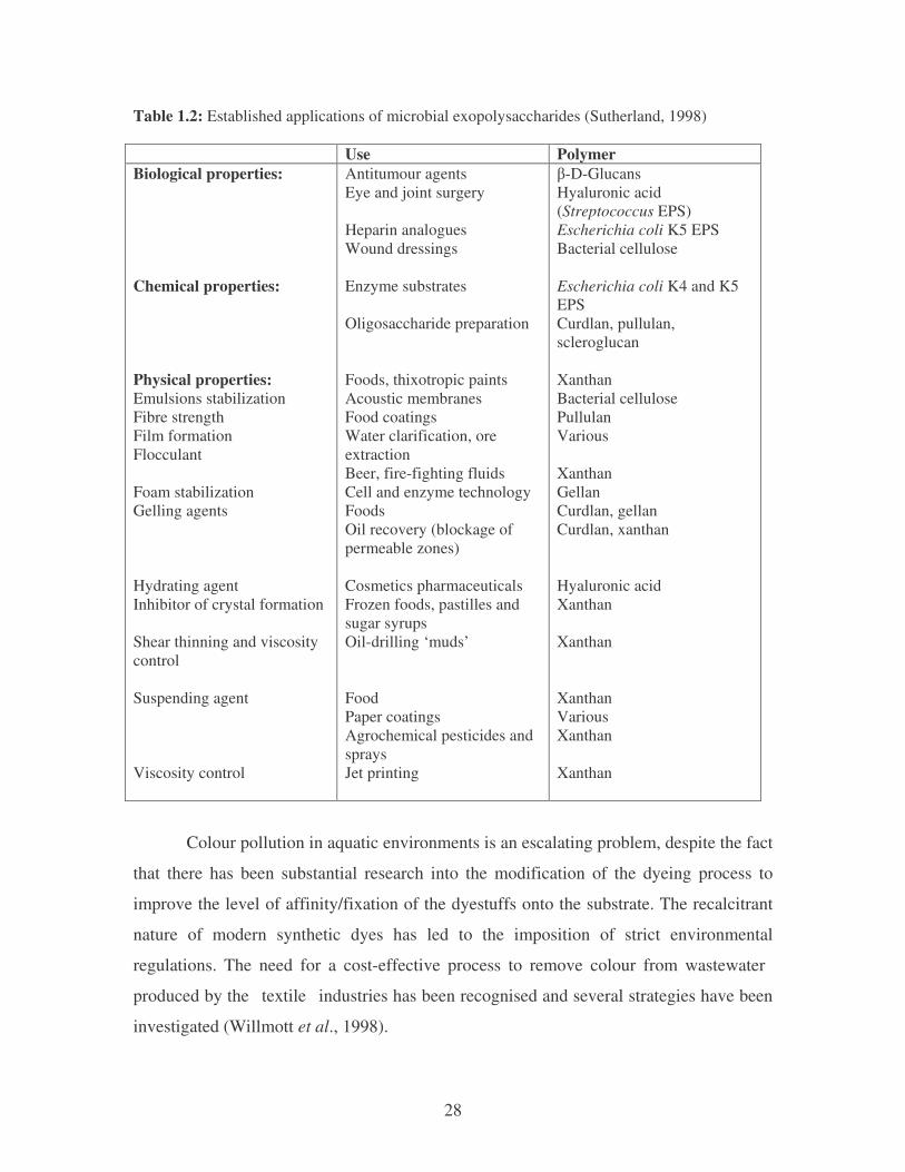
Table 1.2: Established applications of microbial exopolysaccharides (Sutherland, 1998) Use Polymer Biological properties: Chemical properties: Physical properties: Emulsions stabilization Fibre strength Film formation Flocculant Foam stabilization Gelling agents Hydrating agent Inhibitor of crystal formation Shear thinning and viscosity control Suspending agent Viscosity control
Antitumour agents Eye and joint surgery Heparin analogues Wound dressings Enzyme substrates Oligosaccharide preparation Foods, thixotropic paints Acoustic membranes Food coatings Water clarification, ore extraction Beer, fire-fighting fluids Cell and enzyme technology Foods Oil recovery (blockage of permeable zones) Cosmetics pharmaceuticals Frozen foods, pastilles and sugar syrups Oil-drilling ‘muds’ Food Paper coatings Agrochemical pesticides and sprays Jet printing
�-D-Glucans Hyaluronic acid (Streptococcus EPS) Escherichia coli K5 EPS Bacterial cellulose Escherichia coli K4 and K5 EPS Curdlan, pullulan, scleroglucan Xanthan Bacterial cellulose Pullulan Various Xanthan Gellan Curdlan, gellan Curdlan, xanthan Hyaluronic acid Xanthan Xanthan Xanthan Various Xanthan Xanthan
Colour pollution in aquatic environments is an escalating problem, despite the fact
that there has been substantial research into the modification of the dyeing process to
improve the level of affinity/fixation of the dyestuffs onto the substrate. The recalcitrant
nature of modern synthetic dyes has led to the imposition of strict environmental
regulations. The need for a cost-effective process to remove colour from wastewater
produced by the textile industries has been recognised and several strategies have been
investigated (Willmott et al., 1998).
29
Chlorine is widely used in the treatment of water for both industrial and domestic
purposes. Chlorination of water results in formation of an array of disinfection by-
products (DBPs). Trihalomethanes (THMs) are the most common volatile DBPs and
haloacetic acids (HAAs) are the major non-volatile DBPs. Other DBPs, such as,
haloacetonitriles (HANs), chloropicrine and chlorinated furanones, are usually present at
lower concentrations. Health effects of exposures to DBPs include various cancers and
reproductive health effects, including spontaneous abortions, stillbirths, congenital
malformations and retarded fetal development (Egorov et al., 2003). Therefore, the
development of safe and biodegradable flocculant agents that will minimize the
environmental and health risk is of paramount importance in various industries. Hence,
the current study will focus on investigating the role of bacterial bioflocculants in the
reduction and removal of microbial load and textile industrial effluents.
1.8.1 Hypotheses to be tested
It is hypothesized that bacterial bioflocculants can significantly reduce the
microbial load in river water as well as remove a variety of dyes and chemicals from
textile industrial effluents.
1.8.2 Objectives
a. To isolate and characterize the properties of the bioflocculants from bacteria.
b. To evaluate the efficacy of the bacterial bioflocculant on decreasing the microbial load
of river water and compare the findings to alum.
c. To evaluate the ability of the bacterial bioflocculants to remove dyes and chemicals
from the industrial effluents.
1.8.3 Key questions
a. Do all bacterial strains found in wastewater produce extracellular polysaccharides?
b. What is the chemical composition and properties of these bacterial bioflocculants?
30
c. What are the factors that influence bioflocculation?
d. Can these bioflocculants be used as an alternative to alum?
e. Can these bacterial bioflocculants remove dyes from textile industrial effluents?
31
CHAPTER TWO
PRODUCTION AND CHARACTERIZATION OF BACTERIAL
BIOFLOCCULANTS
2.1 INTRODUCTION
Microbial extracellular polysaccharides (EPS) or extracellular biopolymeric
flocculants (EBFs) are either associated with, and often covalently bound to, the cell
surface in the form of capsules, or secreted into the environment in the form of slime.
They are referred to as capsular (CPS) or slime (EPS) exopolysaccharides, respectively.
Cell wall polysaccharides (WPS) are another type that, in contrast to EPS, are not
released into the medium and are associated with the cell envelope, and may again be
either covalently bound to the peptidoglycan layer or loosely associated with it. The lack
of economical production limits their use and consequently they represent a small
fraction of today’s biopolymer market. Efficient production and reduction in recovery
costs requires knowledge of biosynthesis and adoption of appropriate bioprocess
technologies (De Vuyst et al., 2001).
Understanding and controlling the important environmental variables affecting
polymer synthesis can be advantageous in the design of an economic process. The basic
carbohydrate structure of most exopolysaccharides does not change with growth
conditions, but the content of groups attached to the basic carbohydrate structure, can
vary widely and may have a dramatic effect on the properties of the polymer and hence
their effectiveness in various applications (Lopez et al., 2003). For the production of
these biopolymer flocculants, sugars such as glucose, fructose or sucrose (Takagi and
Kodowaki, 1985; Kurane et al., 1986b; Kurane and Nohata, 1991; Toeda and Kurane,
1991), casein, L-glutamate or citrate are usually required as the main substrate(s).
Polysaccharides, which constitute the outermost layer of cells, are thought to
mediate interaction between cells or the adherence of cells to surfaces. Some
32
polysaccharides are liberated outside of the cell, and some are bound to the cell envelope,
but under certain physiological conditions, extracellular polysaccharide molecules may
remain bound and associated with the cell surface without detectable membrane
anchoring. The function of the extracellular polysaccharide in flocculation and adhesion
is an important theme as is the function of envelope bound polysaccharides (Nakata and
Kurane, 1999).
Bioflocculants are essentially polymers produced by microorganisms during
growth, with their flocculating activities being dependent on the characteristics of the
flocculants. Most bioflocculants are reported to comprise of polysaccharides and proteins.
For example, Bacillus subtillis (Yokoi et al., 1996a ), Bacillus licheniformis (Shih et al.,
2001), Paecilomyces sp. (Shubo et al., 2005) and Nocardia amarae YK1 (Takeda et al.,
1992) produce proteinaceous bioflocculants. Alcaligenes latus KT201 (Toeda and
Kurane, 1991) and Enterobacter sp. (Yokoi et al., 1997) produce polysaccharide
bioflocculants, while glycoprotein bioflocculants are produced by Arcuadendron sp. TS-4
(Lee et al., 1995).
In proteinaceous bioflocculants, the amino and carboxyl groups are the effective
groups for flocculation, and their molecular weights are usually low (Kurane et al.,
1994a). In contrast, polysaccharide bioflocculants have high molecular weights and many
functional groups (Kurane et al., 1991). The molecular weight of most bioflocculants
reported in the literature is in the range of 105 to 2.5 × 10⁶ Da (Salehizadeh and
Shojaosadati, 2001). The components and structures of bioflocculants are complex, with
different organisms producing various bioflocculants with diverse properties. The
bridging mechanism was found to play an important role in flocculating organic particles
in wastewater and yeast cells using the bioflocculants produced by Bacillus
mucilaginosus and Aspergillus sojae (Deng et al., 2003). Charge neutralization occurs
when the flocculant is oppositely charged compared to the particles. As most
bioflocculants and particles are negatively charged, charge neutralization seldom occurs
in the bioflocculation process. Compared with conventional chemical and synthetic
flocculants, which are relatively well developed, and their flocculating mechanisms
33
(including bridging and charge neutralization) well understood, the flocculating
mechanisms of bioflocculants still needs to be investigated (Zouboulis et al., 2004).
Many microorganisms secrete EBFs in the culture broth. Bioflocculation resulting
from synthesis and secretion of EBFs by microorganisms has been well known in
activated sludge (Salehizadeh and Shojaosadati, 2001). Generally, soil and activated
sludge samples are the best sources for isolating EBF-producing microorganisms.
Rhodococcus erythropolis was isolated from activated sludge using phthalic acid
assimilation as an indicator (Kurane and Matsuyama, 1994).
Many factors influence the production of EBFs and the bioflocculation process.
These include genotypic, physiological and environmental aspects. The environmental
aspects involve physical, chemical and biological factors. The carbon and nitrogen
concentration (C/N ratio), culture pH, temperature, and agitation speed used in the
fermentor need to be optimized for efficient production (Salehizadeh and Shojaosadati,
2001). This optimization is essential because productivity and distribution of EBFs
depend on the culture conditions. The pH of the culture medium can influence the
production of EBFs. For example, in one case, the localization of the flocculant on the
cell’s surface of Aspergillus sojae at pH 6 was greater than at pH 8. In the case of C.
xerosis, the flocculant was produced at relatively low pH whereas the optimum pH for
production of EBF by A. sojae was in the alkaline range. Temperature is another physical
factor that affects the production of EBFs. The best production of EBFs by A. sojae was
obtained within the temperature range of 30–34oC. The interaction between different
microorganisms in a mixed culture is another biological parameter that can have a
positive effect on aggregation of cells and the production of EBFs (Nakamura et al.,
1976c). By adjusting the growth conditions, the adsorption of the flocculant F-1 on the
cell’s surface could be raised by 5% of the concentration in the filtrate (Nakamura et al.,
1976c).
The importance of carbon and nitrogen sources and the C/N ratio has been
emphasized for EBFs production (Nakamura et al., 1976c; Kurane et al., 1994a). The
34
addition of sugars to the medium reduced the pH of the culture broth and inhibited the
accumulation of the flocculant. Ethanol is also a good carbon source for flocculant
production on an industrial scale (Nakata and Kurane, 1999). The canning factories
wastes and spillage from distilleries are alternative inexpensive carbon sources. Urea,
ammonium sulphate, yeast extract, and casamino acids are good nitrogen sources for EBF
production and growth of R. erythropolis (Tong et al., 1999).
The application potential of EBF is determined by their physical and rheological
properties. Factors influencing these properties are molecular mass, stiffness of the
polymer, presence of side chains, and presence of nonsaccharide components, such as
organic (e.g., acetyl, pyruvyl, or succinyl groups) or inorganic (e.g., sulphate or
phosphate groups) substituents. Genetic engineering may be applied as a tool to direct the
EPS synthesis and introduce desired properties by altering the composition or chain
length. This requires a proper understanding of the genetics and biochemistry of EPS
biosynthesis (Van-Kranenburg et al., 1999).
Inorganic and organic synthetic polymer flocculants are frequently used in water
and wastewater treatment because they are economical and highly effective. However,
their use often gives rise to environmental and health problems in that some of them are
not readily biodegradable and some of their degraded monomers, such as acrylamide, are
neurotoxic and even strong human carcinogens. Residual alum concentration in treated
water can also impose health problems apart from the production of high amount of
sludge (Letterman and Driscoll, 1988). There is also a problem of reaction of alum with
natural alkalinity present in water leading to a reduction of pH and a low efficiency in
coagulation of cold waters (Degremont, 1989 − cited by Ndabigengesere and Narasiah,
1998). Thus, the development of safe biodegradable flocculants that will minimize
environmental and health risks is urgently required (Shih et al., 2001). Hence, the
objective of this chapter were to isolate and identify bacteria capable of bioflocculant
production; to quantify the amount of flocculant produced by the bacteria; and to
characterize the properties of the bioflocculants produced by these bacteria isolated from
the wastewater treatment plant.
35
2.2 MATERIALS AND METHODS
2.2.1 Isolation and identification of bioflocculant producing bacteria
2.2.1.1 Isolation and biochemical characterization of the bacterial
isolates
Microorganisms were isolated from the effluent samples collected from various
points at the Northern Wastewater Treatment Plant, Durban, including; activated sludge
(aerobic), activated sludge (anaerobic), digested sludge, and effluent clarifier. Pure
cultures were obtained by using four way streaks on nutrient agar and dilution methods
(Prescott et al., 1996). Bacterial isolates were maintained on YMPG agar. Bacterial
strains were identified and characterized using standard biochemical tests with reference
to Bergey’s Manual of Systematic Bacteriology (Peter et al., 1986; Garrity, 2005) and the
API Kit (Biomerieux).
2.2.1.2 DNA isolation and 16S rDNA gene amplification and
sequencing
Total genomic DNA was isolated from LB-grown cells using QIAamp DNA
Miniprep Kit (Qiagen) following manufacture’s instructions, and used directly as the
template for PCR amplification. The 16S rDNA of the bacterial isolates were amplified
with the oligonucleotide primers: 63f (5'–CAGGCCTAACACATGCAAGTC-3') and
1387r (5'–GGGCGG(A/T)GTGTACAAGGC-3') [numbering based on the E. coli 16S
rRNA gene (Brosius et al., 1978)] described by Marchesi et al. (1998). The amplification
reaction mixture contained standard Taq amplification buffer, 100 �M (each)
deoxyribonucleotide triphosphate, 0.5 �M (each) primer, 100 ng of genomic DNA and
2.5 U of Taq DNA polymerase in a 50 �l reaction volume. The cycling parameters were
94oC for 2 min followed by 30 cycles of denaturation at 92oC for 30 s, annealing at 55oC
for 30 s, and elongation at 75oC for 45 s, with a final elongation step of 75oC for 5 min.
The PCR products obtained above were visualized in 1% agarose by horizontal
36
electrophoresis at 80 V for 2 hrs. The agarose gels were stained in 0.5 �g/ml ethidium
bromide solution for 15 min and fluorescent bands visualized under a UV
transilluminator (UVP Inc.). The PCR products were sent to Inqaba Biotech for
sequencing. Similarity searches in DNA data bases were perfomed using BLAST analysis
(Pubmed).
2.2.2 Measurement of bioflocculant production
Microorganisms were cultivated in 250 ml Erlenmeyer flasks containing 30 ml
YMPG medium for 20 hrs at 28oC on a rotary shaker at 220 rpm. A 0.7 ml aliquot was
added into a 500 ml Erlenmeyer flask containing 70 ml of production medium (0.5%
yeast extract, 0.5% polypeptone, 2% ethanol, 1% glycerol, 0.05% K2HPO4, 0.05%
MgSO4.7H2O, 0.2% NaCl, and 0.2% CaCO3). The flasks were incubated for 3 days at
28oC before determining the amount of bioflocculant produced by the ethanol
precipitation method (Kurane et al., 1994a).
2.2.3 Bioflocculant purification
In order to purify the biopolymer flocculant, the viscous culture broth was diluted
with an equal volume of distilled water and centrifuged at 2800 ×g for 30 min to remove
cell pellets. Two volumes of cold ethanol (4oC) was added to the supernatant and the
crude bioflocculant precipitate was dried in a dessicator overnight. Thereafter, the crude
bioflocculant was dissolved in distilled water and 2% (w/v) cetylpyridinium chloride
solution (CPC) was added until no more insoluble CPC-bioflocculants complex were
formed. After several hours, the precipitate collected by centrifugal separation of the
CPC-bioflocculants complex was dissolved in saline solution [0.85% (w/v) NaCl],
washed with cold ethanol three times and lyophilized (Salehizadeh and Shojaosadati,
2002).
37
2.2.4 Analysis of the bioflocculants
2.2.4.1 Determination of carbohydrate, protein, uronic acid, and
amino sugar content of the purified bioflocculants
The total sugar content of the purified bioflocculants was determined by the
phenol-sulphuric acid method (Chaplin, 1994). The Folin-Lowry method was used to
measure the total protein content of the bioflocculants (Plummer, 1978). Aromatic amino
acids and �-amino acids were determined by xanthoprotein and ninhydrin reactions
(Plummer, 1978). Amino sugars were determined by the Elson-Morgan method (Chaplin,
1994). The carbazol method was used to measure uronic acid (Chaplin, 1994). Full
description of the methodology and data sets obtained are given in Appendix B.
2.3 RESULTS
2.3.1 Bacterial isolation and identification
Of the thirty bioflocculant producing bacteria initially isolated from the
wastewater treatment plant, only six were selected on the basis of the amount of
bioflocculant produced (the highest, intermediate and the lowest producers) were used in
subsequent experiments. The biochemical tests and the API Kit (Appendix A Table 6.1)
were used to tentatively identify the organisms up to the genus level, and then confirmed
by the analysis of their 16S rRNA gene sequences. Figure 2.1 shows the amplicons of
16S rDNA genes of the bacterial isolates. The analysis of the gene sequences (shown in
Appendix A) identified the bacterial isolates as indicated in Table 2.1
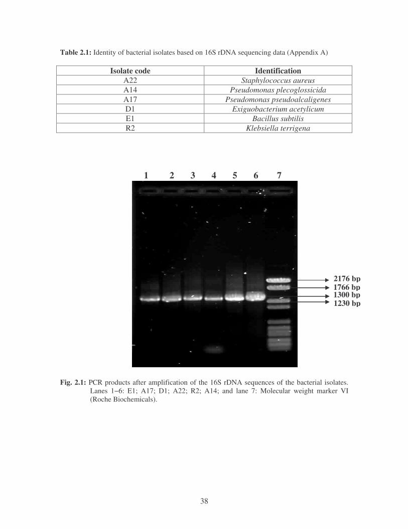
38
Table 2.1: Identity of bacterial isolates based on 16S rDNA sequencing data (Appendix A)
Isolate code Identification A22 Staphylococcus aureus A14 Pseudomonas plecoglossicida A17 Pseudomonas pseudoalcaligenes D1 Exiguobacterium acetylicum E1 Bacillus subtilis R2 Klebsiella terrigena
1 2 3 4 5 6 7
Fig. 2.1: PCR products after amplification of the 16S rDNA sequences of the bacterial isolates.
Lanes 1−6: E1; A17; D1; A22; R2; A14; and lane 7: Molecular weight marker VI (Roche Biochemicals).
1300 bp
1230 bp
2176 bp 1766 bp
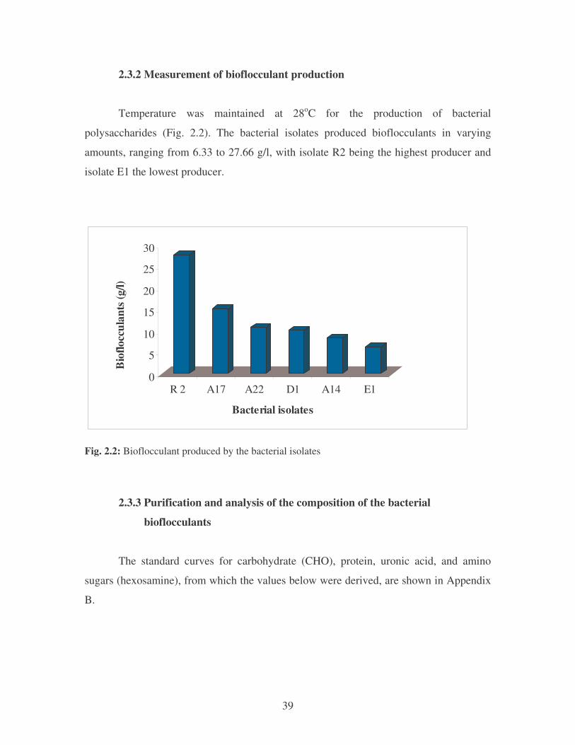
39
2.3.2 Measurement of bioflocculant production
Temperature was maintained at 28oC for the production of bacterial
polysaccharides (Fig. 2.2). The bacterial isolates produced bioflocculants in varying
amounts, ranging from 6.33 to 27.66 g/l, with isolate R2 being the highest producer and
isolate E1 the lowest producer.
0
5
10
15
20
25
30
Bio
flocc
ulan
ts (g
/l)
R 2 A17 A22 D1 A14 E1
Bacterial isolates
Fig. 2.2: Bioflocculant produced by the bacterial isolates
2.3.3 Purification and analysis of the composition of the bacterial
bioflocculants
The standard curves for carbohydrate (CHO), protein, uronic acid, and amino
sugars (hexosamine), from which the values below were derived, are shown in Appendix
B.
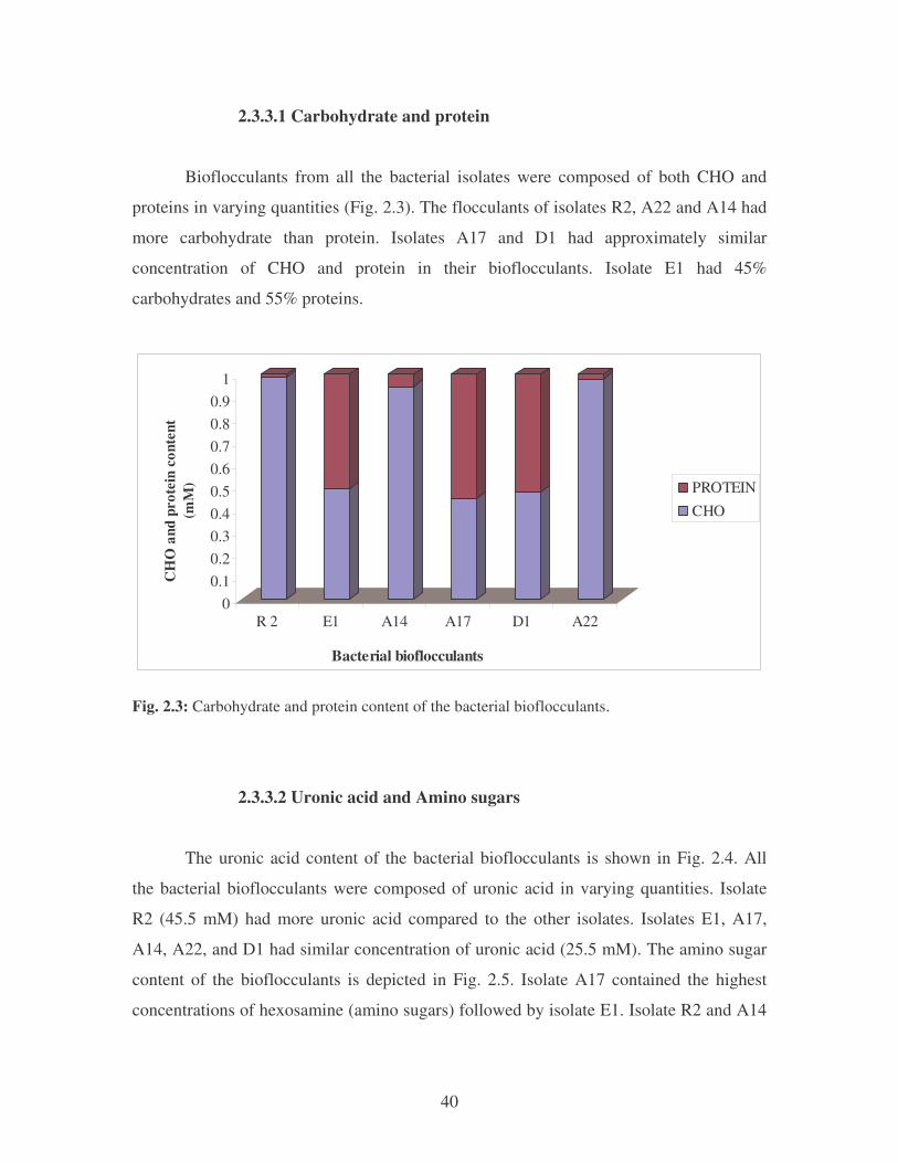
40
2.3.3.1 Carbohydrate and protein
Bioflocculants from all the bacterial isolates were composed of both CHO and
proteins in varying quantities (Fig. 2.3). The flocculants of isolates R2, A22 and A14 had
more carbohydrate than protein. Isolates A17 and D1 had approximately similar
concentration of CHO and protein in their bioflocculants. Isolate E1 had 45%
carbohydrates and 55% proteins.
00.10.20.30.40.50.60.70.80.9
1
CH
O a
nd p
rote
in c
onte
nt
(mM
)
R 2 E1 A14 A17 D1 A22
Bacterial bioflocculants
PROTEINCHO
Fig. 2.3: Carbohydrate and protein content of the bacterial bioflocculants.
2.3.3.2 Uronic acid and Amino sugars
The uronic acid content of the bacterial bioflocculants is shown in Fig. 2.4. All
the bacterial bioflocculants were composed of uronic acid in varying quantities. Isolate
R2 (45.5 mM) had more uronic acid compared to the other isolates. Isolates E1, A17,
A14, A22, and D1 had similar concentration of uronic acid (25.5 mM). The amino sugar
content of the bioflocculants is depicted in Fig. 2.5. Isolate A17 contained the highest
concentrations of hexosamine (amino sugars) followed by isolate E1. Isolate R2 and A14
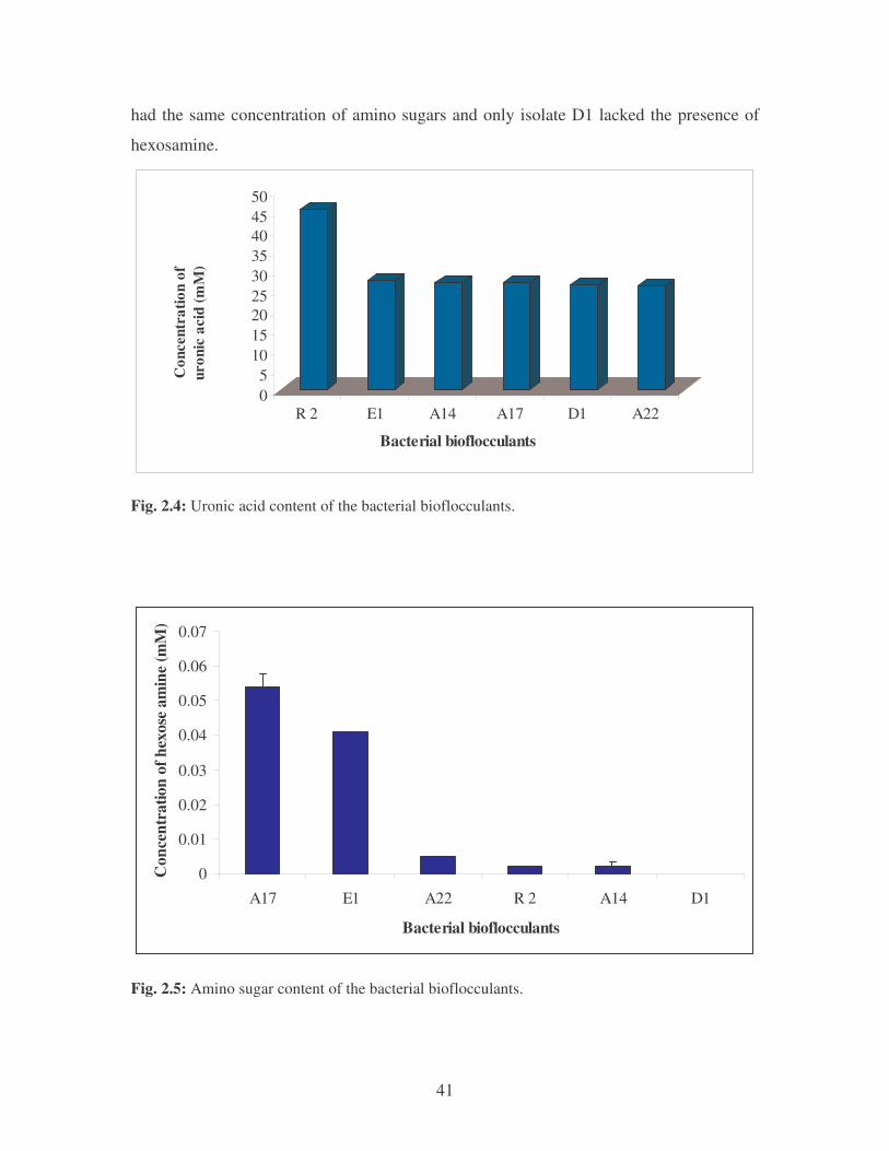
41
had the same concentration of amino sugars and only isolate D1 lacked the presence of
hexosamine.
05
101520253035404550
Con
cent
ratio
n of
ur
onic
aci
d (m
M)
R 2 E1 A14 A17 D1 A22
Bacterial bioflocculants
Fig. 2.4: Uronic acid content of the bacterial bioflocculants.
0
0.01
0.02
0.03
0.04
0.05
0.06
0.07
A17 E1 A22 R 2 A14 D1
Bacterial bioflocculants
Con
cent
ratio
n of
hex
ose
amin
e (m
M)
Fig. 2.5: Amino sugar content of the bacterial bioflocculants.
42
2.4 DISCUSSION
In this study the YMPG medium which contained yeast extract, polypeptone,
glycerol, and ethanol were used as substrates for the production of bacterial
bioflocculants. Yeast extract was a very good organic nitrogen source for the production
of bioflocculants (Fig. 2.2). Nataka and Kurane (1999) indicated that polypeptone and
yeast extract were good nitrogen sources for the production of EPS by Klebsiella
pneumoniae H12. Kurane et al. (1994a) determined ethanol to be the cheapest substrate
for bioflocculant production. According to Nakamura et al. (1976c) and Kurane et al.
(1994a) the production of EPS by A. sojae was enhanced when casein, yeast extract,
polypeptone, and some amino acids (e.g. glutamic acid and alanine) were added to the
medium.
The six bacterial isolates investigated in this study produced extracellular
polysaccharide/bioflocculants in varying quantities (Fig. 2.2). Isolate R2 (K. terrigena)
produced 27.66 g/l while the production by D1 (E. acetylicum) was 10.167 g/l. The
lowest producer was isolate E1 (B. subtilis) which produced only 6.33 g/l. Salehizadeh
and Shojaosadati (2002) reported that 1.36 g/l of crude bioflocculant was produced by
Bacillus firmus. This amount is much lower than that produced by B. subtilis in this
study. In a similar study done by Shih et al. (2001), 14 g/l of crude bioflocculant was
produced by Bacillus licheniformis CCRC 12826 which was higher than that produced by
isolate B. subtilis. Only 3 g of bacterial bioflocculant was produced by K. pneumoniae
H12 in a study done by Nakata and Kurane (1999). The amount produced by this
bacterium is lower than that produced by isolate R2 (K. terrigena). This may be due to
the fact that different species of Klebsiella were used. Zouboulis et al. (2004) reported on
the production of bioflocculant by the bacterium Rhizomonas sp.; and have shown that
only 2 g of bioflocculant were produced. Amongst the five genera used in the present
study (Table 2.1) only four have been extensively studied previously, namely, Bacillus
sp. (Kim, 1993; Yokoi et al., 1995, 1996a; Suh et al., 1997; Salehizadeh et al., 2000);
Pseudomonas sp. (Tago and Aida 1977); Klebsiella sp. (Dermlim et al., 1999) and
43
Staphylococcus sp. (Nakamura et al., 1976b). Currently there are no reports regarding the
production of bioflocculants by E. acetylicum.
According to the findings of the present study, bacterial bioflocculants were
composed of carbohydrates, proteins, uronic acid, and hexosamine. Isolate R2 and A22
had 99% carbohydrate and 1% protein while isolate D1 and A17 had 40% carbohydrate
and 60% protein in their bioflocculants (Fig. 2.3). In a study done by Fujita et al. (2000)
on the characterization of a bioflocculant produced by Citrobacter TKF04 from acetic
and propionic acids, the total sugar content of the bioflocculant was 10% and no proteins
were detected. A similar study was carried out by Salehizadeh and Shojaosadati (2002)
on the isolation and characterization of bioflocculant produced by B. firmus. The
bioflocculant was composed of 87% total sugar, 38% uronic acid and no proteins were
detected (Fig. 2.4). Shubo et al. (2005) indicated that bioflocculant produced by
Aspergillus parasiticus had 76.3% sugar content and a 21.6% protein. In general,
bacterial bioflocculants contain proteins in minute quantities. Higgins (1995) reported
that extracellular proteins in the floc are associated with improvements in settling and
dewatering properties.
To date, many studies on the microbial production of flocculating substances have
been reported. Microbiologically-produced bioflocculants are generally high molecular-
weight polymers, and have been identified or presumed to be proteins (Takeda et al.,
1991; Takeda et al., 1992), glycoproteins (Kurane et al., 1986b), polysaccharides
(Kurane and Nohata, 1991; Toeda and Kurane, 1991), glycolipids (Kurane et al., 1994a),
cellulose (Napoli et al., 1975), DNA (Sakka and Takahashi, 1981) or complex hetero-
polymers (Nakamura et al., 1976a). The primary structure of proteins and
polysaccharides describes the arrangement of the different building blocks, amino acids
and monosaccharides, respectively, along the polymer chain. The possible structural
variability due to available units and connecting patterns is estimated to be about three
orders of magnitude larger for polysaccharides than for proteins (Sletmoen et al., 2003).
44
In this study, all the bacterial bioflocculants were composed of uronic acid in
varying quantities. Isolate R2 had the highest concentration of uronic acid [45.3 mM]
(Fig. 2.4) compared to the other bacterial isolates. Nakata and Kurane (1999) showed that
the bioflocculant produced by K. pneumoniae was composed of only 10% uronic acid.
This amount was very low when compared to that produced by isolate R2 (K. terrigena)
in the current study. Salehizadeh et al. (2000) analyzed the composition of the
bioflocculant produced by Bacillus sp As 101, and indicated that it was composed of only
11.4% uronic acid, this amount was lower than that produce by B. subtilis (25%) in this
study. Uronic acids appear to be the most universal and specific indicators of
extracellular polymers that are used by the invertebrates in feeding nets, faecal
pelletization, or feeding tube structures in the benthic environment and of the polymers
that protect and regulate the ionic traffic at the surface of the bacteria. These polymers are
important in the stabilization of marine sediments. The uronic acid content of the
extracellular polymers can be measured by the formation of the ester and the reduction of
the carboxylic acid moiety to an alcohol. This process eliminates the problems of
resistance to hydrolysis and of quantitative recovery in separation from the neutral
carbohydrates (Fazio et al., 1982). They are also found in the polysaccharide polymers of
higher plant cell walls, in gram-positive microbes under conditions of phosphate
limitation (Elwood and Tempest, 1972), and in some gram-negative microbial
lipopolysaccharides. Polymers containing uronic acid are resistant to quantitative
hydrolysis, and the uronic acid, once released, form lactones irreproducibly and are
difficult to separate from the neutral sugars. Uronic acids are often estimated by their acid
catalyzed decarboxylation under controlled conditions (Kiss, 1974). The known
microbial exopolysaccharides contain D-glucuronic acid, D-galacturonic acid, D-
mannuronic acid, and L-gulonic acid (Dudman, 1977).
Amino sugars are important structural components of bacterial cell walls, and
neutral carbohydrates make up a basic unit of plant cells (Cheng and Kaplan, 2003). Five
of the six bacterial bioflocculants used in this study were composed of hexosamine or
amino sugars in very low concentrations except for isolate D1, which is E. acetylicum.
The small yield might be due to the unstability of the amino sugar or the presence of
45
some reducing substance other than amino sugar in the bioflocculant. This finding is
consistent with that done by Nakata and Kurane (1999); who showed that no hexosamine
was detected in the bioflocculant produced by K. pneumoniae H12. Generally, amino
sugars are present in very small quantities in bacterial cell walls. Fujita et al. (2000)
reported that bioflocculant produced by Citrobacter sp. TKF04 was composed of 29.4%
of hexosamine. In this study, bacterial bioflocculants were produced and characterized.
They were found to be composed of carbohydrate, protein, uronic acid, and hexosamine
in varying quantities.
46
CHAPTER THREE
COAGULATION-FLOCCULATION BY MICROBIAL BIOFLOCCULANTS
3.1 INTRODUCTION
Historically, the term “coagulation” and “flocculation” have been used
indiscriminately to describe the process of removal of turbidity from water. There is
however a clear distinction between the two terms. The term “coagulation” comes from
the Latin coagulare, meaning to drive together (Faust and Aly, 1998; Nester et al., 2001).
This process describes the effect produced by the addition of chemicals to a colloidal
dispersion resulting in particle destabilization by a reduction of the forces tending to keep
the particles apart. Colloidal particles have a net negative surface charge. The size of
colloids (0.001 to 1 �m) is such that the attractive forces between particles are
considerably less than the repelling forces of the electrical charge. Under these stable
conditions, particle growth does not occur, and Brownian motion keeps the particles in
suspension. Operationally, coagulation is achieved by adding appropriate chemicals,
which causes particles to stick together when contact is made. Rapid mixing is important
at this stage to obtain uniform dispersion of the chemical and to increase the opportunity
for particle-to-particle contact. The entire process occurs in a very short time, probably
less than a second, and initially results in particles submicroscopic in size (Cohen et al.,
1972; Prescott et al., 1996). The settling velocities of finely divided and colloidal
particles under gravity alone are so small that ordinary sedimentation is not practical. It is
therefore necessary to use procedures, which agglomerate the small particles into larger
aggregates, which then have the settling velocities required for various applications.
Formation of larger particles from smaller ones is also required for their removal by
filtration (Nester et al., 2001).
The second stage of the formation of settleable particles from destabilized
colloidal-sized particles is termed flocculation. This term also has its derivation from
Latin, flocculare, meaning to form a floc, which visually resembles a tuft of wool or
47
highly fibrous porous structure. In contrast to coagulation, where the primary force is
electrostatic, flocculation occurs by a chemical bridging of physical enmeshment
mechanism. Flocculation is operationally obtained by gentle and prolonged mixing which
converts the submicroscopic coagulated particles into discrete, visible, suspended
particles. At this stage, the particles are large enough to settle rapidly under gravity and
may be removed from suspension by filtration. The more usual practice has been to
physically separate the unit processes into coagulation-flocculation, sedimentation, and
filtration (Cohen et al., 1972; Faust and Aly, 1998).
The chemical coagulation of turbid water or naturally coloured surface water
involves the interaction of particulates and/or colloids with a destabilizing agent. The
essential purpose of coagulation is to aggregate these particles into larger sizes that will
settle quickly within an hour or two and/or will be filtered by sand or other media. This
aggregation process is also called destabilization of colloidal systems. Colloids are
characterized by their size and by the mechanism by which they are stabilized in water.
Another characteristic of colloids is their affinity for the solvent in which stabilization
occurs. This is a process of salvation. Lyophilic is the general term given to colloids
“loving” the solvent. In water, this becomes hydrophilic, and such colloids are stabilized
by the formation of adherent thick layers of oriented water molecules around the particle.
Lyophobic is the general term given to colloids “hating” the solvent, which in water
becomes hydrophobic; such colloids are stabilized by an electrostatic repulsion between
the particles arising from ions that are attracted to the surface from bulk solution or
dissolved out of the solid’s surface (Bitton, 1994).
Recently there has been a large increase in the utilization of synthetic organic
polymers in the treatment of water and wastewaters as coagulants or aids to coagulation.
Optimum treatment is frequently obtained with anionic and polymeric destabilization of
negatively charged particles. It is obvious that an electrostatic mechanism is not the only
means of destabilization. A bridging theory was proposed by La-Mer and Healy (1963) to
account for the destabilization of colloidal systems by high molecular weight organic
polymers. Adsorption of the polymer on specific sites of the colloid plays an important
48
role in the bridging theory. This theory resembles the binder theory proposed for alum
precipitation and coagulation. In order for a polymer molecule to be an effective
destabilizer, it must contain constituents that can interact with sites on the colloidal
particle (Singh et al., 2000).
A number of methods and/or chemicals are used either as aids to coagulation or as
the primary coagulant. Polyelectrolytes are mostly synthetic organic compounds of high-
molecular weight. They are polymers composed of a chain of monomers. In turn, these
monomers are varied frequently within a given polymer, which results in compounds
with different molecular weights. These polymers are linear or branched. If the monomer
contains an ionisable group, such as carboxyl, amino, or sulfonic, then the polymer is
called a polyelectrolyte. There are cationic, anionic, or ampholytic (has both positive and
negative) groups which, of course, depends on the nature of the functional groups within
the monomer. Non-ionic polymers are those compounds without any ionisable groups.
These polymers and polyelectrolyte are able to flocculate colloidal particles due to
adsorption. In most cases, the bonding mechanism between a functional group on the
polymer and a site on a colloid’s surface is quite specific. In addition, molecular weight
and degree of branching of the polymer play a mechanistic role in their ability to
flocculate (Bitton, 1994; Faust and Aly, 1998).
The rate of flocculation is determined by the collision frequency induced by the
relative motion. Because Brownian movement causes this, it is called perikinetic
flocculation. That which is caused by velocity gradients is called orthokinetic
flocculation. If there is no surface, repulsion between the particles, then every collision
leads to aggregation and the process is called rapid flocculation. If a significant repulsion
exists, then only a fraction of the collisions results in aggregation. This is called slow
flocculation. The floc blanket clarifier provides a special case of orthokinetic
flocculation. In addition to the fluidized bed giving rise to velocity gradients, the
fluidized particles are participating in the process of agglomeration. If particles are
settling at different velocities, then the faster settling particles may collide with slower
settling particles, leading to aggregation. The aggregates will then settle faster due to
49
their increased mass, and possibly experience further collisions and aggregations (Yan et
al., 2004).
Compared with present understanding of floc formation through perikinetic and
orthokinetic mechanisms, understanding of floc breakup in agitated systems is qualitative
and speculative, despite research efforts (Faust and Aly, 1998; Nester et al., 2001).
Proper characterization of floc disruption is an important problem since it is well
documented that break-up can appreciably affect the performance of solid-liquid
separation processes downstream. Floc break-up in dilute agitated suspensions is
governed by the interaction of individual flocs with fluid forces. Depending on its
constituent materials, a floc can be viewed roughly as an aggregate of primary micro
particles that are bound together to form a matrix possessing a substantial fraction of fluid
within its framework. The size and compactness of the matrix, size, and shape of the
microparticles contribute to floc structure and the ability to withstand disruption by fluid
forces. This also includes the number and strength of bonds that the microparticle
contacts (DiTerlizzi and Fall, 1994; Singh et al., 2000).
The biopolymers in activated sludge flocs appear to affect the physico-chemical
properties associated with the flocs such as floc density, floc particle size, specific
surface area, charge density, bound water content, and hydrophobicity. These
physicochemical floc characteristics express themselves among other things as activated
sludge settling and dewatering properties. Research indicates that an increase in floc
density and floc particle size increases settling velocity. The theoretical basis for
improved settling through an increase in floc density and floc particle size is presented in
Stokes Law. An increase in floc density results in improved dewatering properties
through a decrease in bound water associated with the flocs (Eriksson and Alm, 1991).
Calcium may create denser sludge flocs through a decrease in bound water associated
with the floc. The percentage bound water associated with the floc is also an indicator of
the maximum dryness that can be achieved in the sludge cake by mechanical means
(Foster, 1983).
50
A variety of flocculants, including inorganic flocculants (polyaluminium chloride
and aluminium sulphate), organic flocculants (polyacrylamide, polyethylene imine), and
natural flocculants or bioflocculants (gelatin, chitosan guar gum and microbial
flocculants) have been widely used for tap water production, wastewater treatment,
dredging, downstream processing, fermentation, and in the food industry (Zouboulis et
al., 2004, Crini, 2006).
Kaolin’s are white raw materials, their essential constituent being fine grained
white clay which are amenable for beneficiation that make them ideal for an assortment
of industrial applications. Kaolin deposits can be classified into two types, primary
(residual) and secondary (sedimentary) (Prasad et al., 1991). Kaolin or china clay is a
versatile industrial mineral and one of the highest value additions is achieved when it is
beneficiated to pigment grade suitable for paper and paint industries. In kaolin, minor
quantities of transition elements such as iron, titanium, and manganese are generally
present as ancillary minerals, which adversely affect its optical properties (Chandrasekhar
and Ramaswamy, 2006). The valence state of the ion and atomic position in the structure
depend on the conditions of formation of the mineral (Muller et al., 1995). Extensive
research has been carried out on the nature of iron impurities in kaolin, which leads to the
conclusion that iron is present as a part of the kaolinite or ancillary mineral structure i.e.,
“structural iron” or as separate iron minerals such as oxides, hydroxides, oxy-hydroxides,
sulphides and carbonates i.e., free iron. Clay particles are strongly anisotropic and exhibit
faces and edges, which are very different in surface area and in chemical behaviour. The
explanation for dispersion of clay minerals suspensions in water is usually done by
considering that the surfaces are electrically charged. Kaolin clay has been widely used as
a test sample or material for flocculation because of its characteristics (Konan et al.,
2006). Therefore, the objective of this chapter was to evaluate the ability of the bacterial
bioflocculants to flocculate kaolin clay and determine the effects of temperature, pH and
metal salts on the flocculating activities.
51
3.2 MATERIALS AND METHODS
3.2.1 Determination of the growth patterns of bacterial isolates and
measurement of flocculating activity
The flocculating activity of the bacterial isolates was evaluated by
measurement of the turbidity of a kaolin suspension. In all the experiments, 9 ml of
kaolin suspension (5.5 g/l) was mixed with 1 ml of 0.5 M CaCl2 in 9 mM glycine-NaOH
buffer (pH 7.0) in a test tube. The six bacterial cultures used to produce bioflocculants in
this study were grown in 250 ml of YMPG medium for 84 hrs, at 28oC with shaking (150
rpm). Culture broth (50 µl) was then added to the kaolin suspension every 12 hrs for 84
hrs. The test tube was mixed vigorously for 20 s and left to stand, without shaking, for 5
min. The turbidity of the sample supernatant (A) and a control experiment without the
culture broth (B) were measured at 550 nm with spectrophotometer (LKB ultrospec ��)
(Salehizadeh and Shojaosadati, 2002). The flocculating activity was expressed as the
concentration of the flocculant in parts per million (ppm) when the OD550 was (1/10) x
OD550 of the control (Nakata and Kurane, 1999). The percentage removal of kaolin
suspension was calculated by the equations of Kurane and Matsuyama (1994) and Kurane
et al. (1994b) as follows:
Removal (%) = 100×−B
AB
In addition, flocculating activity was also determined using various concentrations of
purified bioflocculants instead of the culture broth.
3.2.2 Flocculation of microbial cultures
The following microbial cultures, obtained from the stock culture collection of the
Discipline of Microbiology (Westville campus) UKZN, South Africa were used:
Pseudomonas aeruginosa, Proteus mirabilis, Serratia marcescens, Alcaligenes faecalis,
52
Citrobacter freundii, Bacillus coagulans, Bacillus cereus, Clostridium hystolyticum,
Streptococcus pyogenes, and Saccharomyces cerevisiae. The bacterial isolates used for
the production of flocculants were also used to measure the flocculation of these cultures.
Microbial cultures were cultivated in 30 ml of YMPG medium in 250 ml Erlenmeyer
flasks for 20 hrs at 28oC with shaking (220 rpm). A 10 ml aliquot of the culture was
washed with and suspended in an equal volume of deionised water in a test tube. One-
hundred microlitres of flocculant solution (1 g/l) and then 100 �l of CaCl2 solution (3 g/l)
were added to the test tube. The mixture was vortexed for 5 s and left to stand for 5 min
and the OD measured with a spectrophotometer at 550 nm. Flocculating activity was
compared to the control without the flocculant or CaCl2 (Nakata and Kurane, 1999). The
flocculating activity was determined as described in Section 3.2.1.
3.2.3 Flocculation inhibition assay
One-hundred microlitres of different concentrations of potential inhibitors
(K2HPO4, NaNO3, CH2COONa, Na2CO3, and D-GLU), 100 �l of bioflocculant solution (1
g/l), and 100 �l of CaCl2.2H2O (30 g/l) were added to 10 ml of kaolin suspension (5 g/l)
in a test tube. The mixture was vortexed for 5 s and left to stand for 5 min and the OD
measured with a spectrophotometer at 550 nm. Flocculation activity was compared to the
control without the salts. The flocculating activity was expressed as described in Section
3.2.1.
3.2.4 Flocculating activities of bacterial bioflocculants and alum
In order to compare the flocculating activity of the bioflocculants with alum the
former was substituted with 10 ppm (0.01 g) alum. Different concentrations (10–50 ppm)
of bacterial bioflocculants were added to 500 ml of raw water in 1-litre Erlenmeyer flasks
and left to stand at room temperature for 1 hr. The control was performed without the
addition of bacterial bioflocculants and the OD was determined spectrophotometerically
at 550 nm for all the samples. The flocculating activity was calculated as described in
Section 3.2.1.
53
3.2.5 Determination of the effect of pH, temperature, and cationic/metal salts
on the flocculating activity of bioflocculants
Flocculating activity was determined as described in Section 3.2.1. The pH of the
kaolin suspension was adjusted using 2 N HCl or NaOH to between 6 and 10 in order to
examine the effect of pH on flocculating activity. To determine the effect of temperature
on flocculating activity, the flocculation experiment was conducted at 28oC and 37oC.
Cationic compounds (MgSO4.7H2O, MnCl2.7H2O and CTAB) were added to the mixture
instead of CaCl2.2H2O in order to determine their effect on flocculating activity (Nakata
and Kurane, 1999).
3.3 RESULTS
3.3.1 The growth patterns of the bacterial isolates in YMPG media and
flocculating activities
Figure 3.1 shows the growth patterns of the bacterial isolates in the YMPG
medium. Maximum cell growth was observed for isolate A22 after 24 hrs, after which the
growth decreased and then remained constant. The other five isolates displayed similar
growth patterns. The flocculating activity of the culture broth increased during the
logarithmic phase of growth in YMPG medium and decreased during the late log phase.
The best flocculating activity was observed in isolate A17 after 24 hrs (Fig. 3.2).
Generally, the flocculating activity of the bioflocculants increased to a maximum
before decreasing to a constant level. However, there was no decrease in activity after 84
hrs for isolate E1. The effect of time on the removal of kaolin suspension by crude
bioflocculants is depicted in Fig. 3.3. Isolate A17 removed more kaolin (65%) after 24
hrs compared to the other isolates. The pattern of removal first increased and reached a
maximum after which it decreased and remained constant except for isolate E1 where the
removal of kaolin did not decrease after 84 hrs.
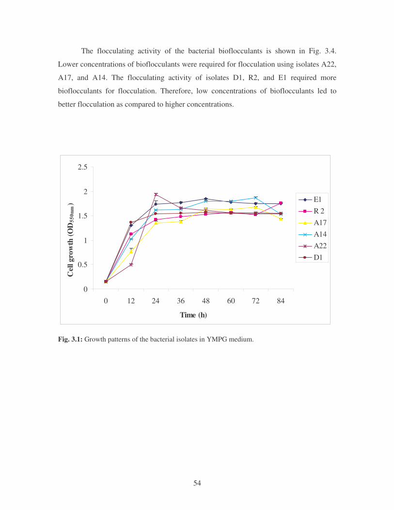
54
The flocculating activity of the bacterial bioflocculants is shown in Fig. 3.4.
Lower concentrations of bioflocculants were required for flocculation using isolates A22,
A17, and A14. The flocculating activity of isolates D1, R2, and E1 required more
bioflocculants for flocculation. Therefore, low concentrations of bioflocculants led to
better flocculation as compared to higher concentrations.
0
0.5
1
1.5
2
2.5
0 12 24 36 48 60 72 84
Time (h)
Cel
l gro
wth
(OD
550n
m) E1
R 2A17A14A22D1
Fig. 3.1: Growth patterns of the bacterial isolates in YMPG medium.
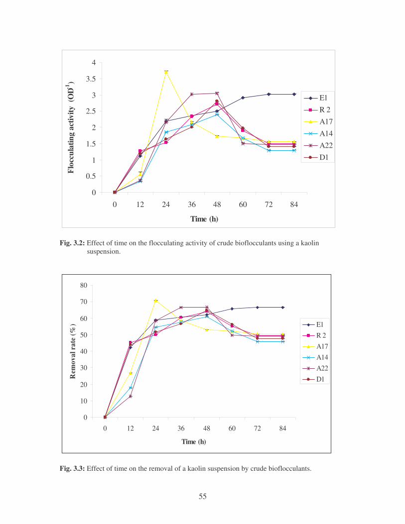
55
0
0.5
1
1.5
2
2.5
3
3.5
4
0 12 24 36 48 60 72 84
Time (h)
Floc
cula
ting
activ
ity (
OD-1
)
E1R 2A17A14A22D1
Fig. 3.2: Effect of time on the flocculating activity of crude bioflocculants using a kaolin suspension.
0
10
20
30
40
50
60
70
80
0 12 24 36 48 60 72 84
Time (h)
Rem
oval
rat
e (%
) E1R 2A17A14A22D1
Fig. 3.3: Effect of time on the removal of a kaolin suspension by crude bioflocculants.
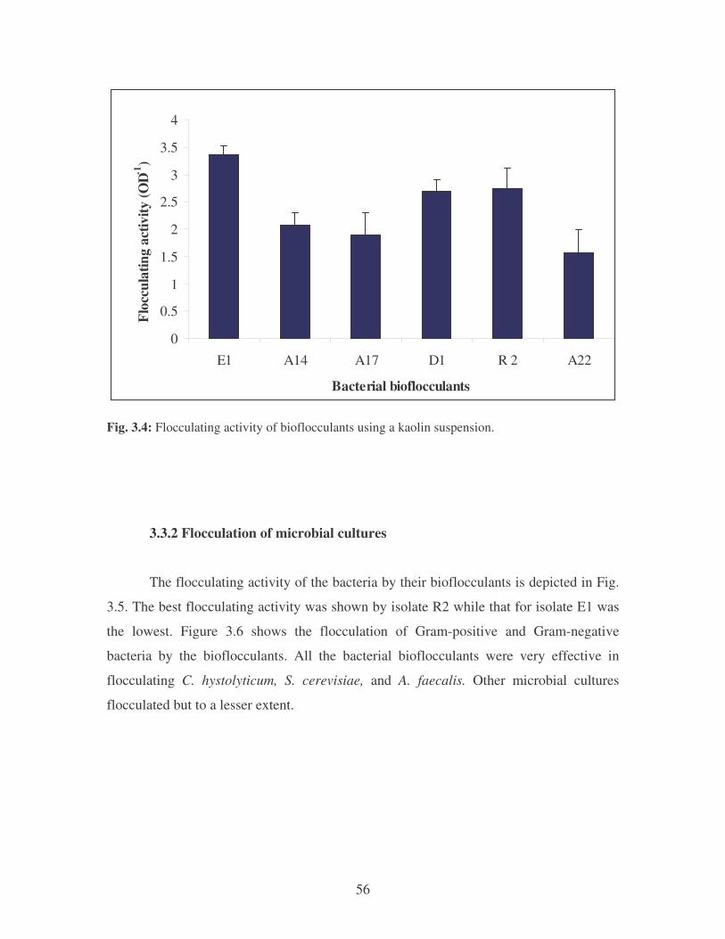
56
0
0.5
1
1.5
2
2.5
3
3.5
4
E1 A14 A17 D1 R 2 A22
Bacterial bioflocculants
Floc
cula
ting
activ
ity (O
D-1)
Fig. 3.4: Flocculating activity of bioflocculants using a kaolin suspension.
3.3.2 Flocculation of microbial cultures
The flocculating activity of the bacteria by their bioflocculants is depicted in Fig.
3.5. The best flocculating activity was shown by isolate R2 while that for isolate E1 was
the lowest. Figure 3.6 shows the flocculation of Gram-positive and Gram-negative
bacteria by the bioflocculants. All the bacterial bioflocculants were very effective in
flocculating C. hystolyticum, S. cerevisiae, and A. faecalis. Other microbial cultures
flocculated but to a lesser extent.
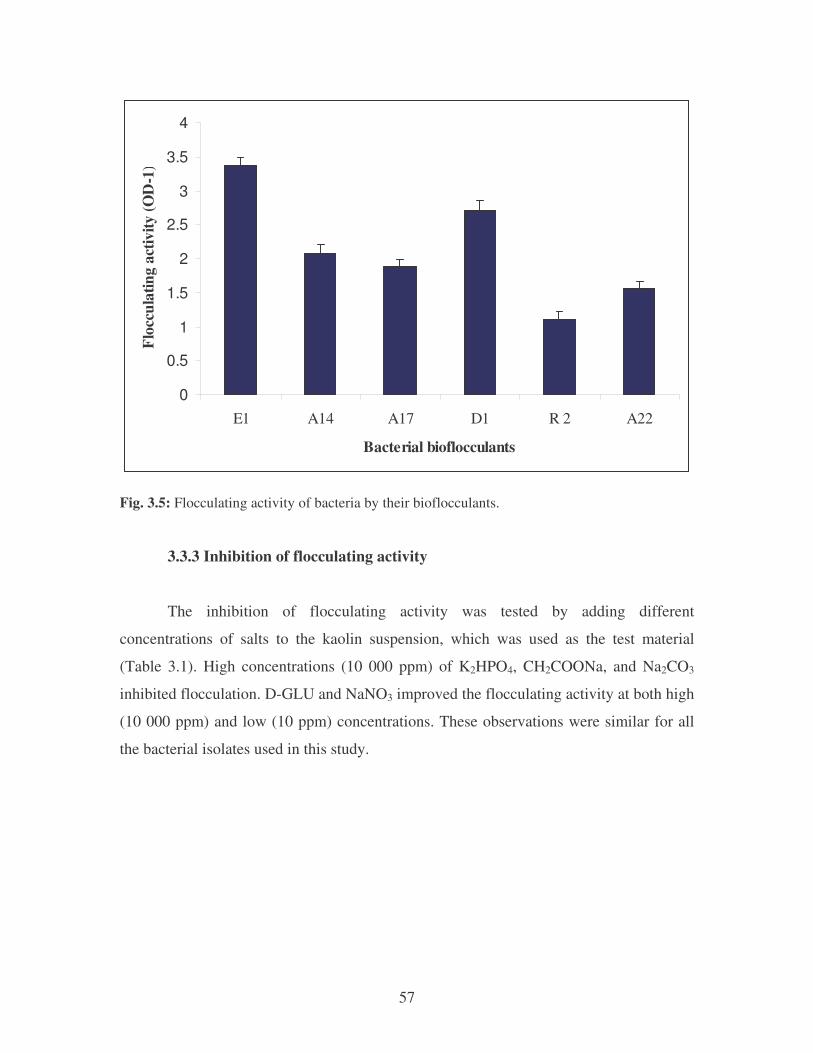
57
0
0.5
1
1.5
2
2.5
3
3.5
4
E1 A14 A17 D1 R 2 A22
Bacterial bioflocculants
Floc
cula
ting
activ
ity (O
D-1
)
Fig. 3.5: Flocculating activity of bacteria by their bioflocculants.
3.3.3 Inhibition of flocculating activity
The inhibition of flocculating activity was tested by adding different
concentrations of salts to the kaolin suspension, which was used as the test material
(Table 3.1). High concentrations (10 000 ppm) of K2HPO4, CH2COONa, and Na2CO3
inhibited flocculation. D-GLU and NaNO3 improved the flocculating activity at both high
(10 000 ppm) and low (10 ppm) concentrations. These observations were similar for all
the bacterial isolates used in this study.
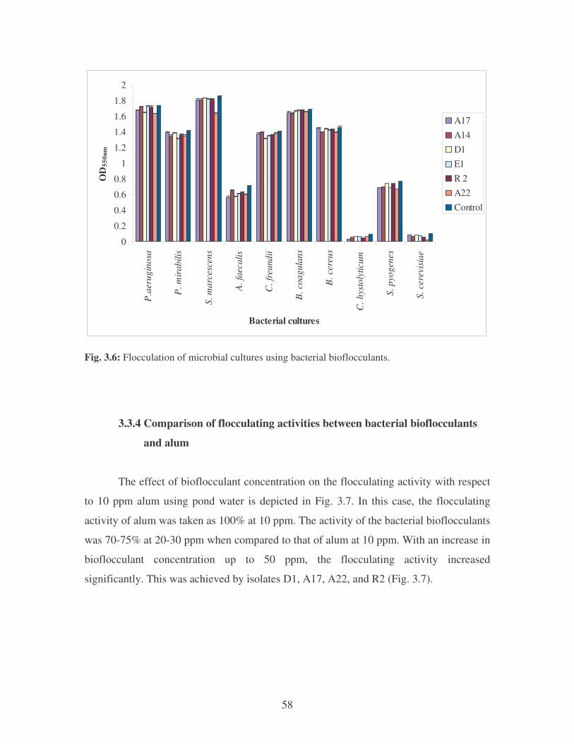
58
0
0.2
0.4
0.6
0.8
1
1.2
1.4
1.6
1.8
2
P.a
erug
inos
a
P. m
irab
ilis
S. m
arce
scen
s
A. f
aeca
lis
C. f
reun
dii
B. c
oagu
lans
B. c
ereu
s
C. h
ysto
lytic
um
S. p
yoge
nes
S. c
erev
isia
e
Bacterial cultures
OD
550n
m
A17A14D1E1R 2A22Control
Fig. 3.6: Flocculation of microbial cultures using bacterial bioflocculants.
3.3.4 Comparison of flocculating activities between bacterial bioflocculants
and alum
The effect of bioflocculant concentration on the flocculating activity with respect
to 10 ppm alum using pond water is depicted in Fig. 3.7. In this case, the flocculating
activity of alum was taken as 100% at 10 ppm. The activity of the bacterial bioflocculants
was 70-75% at 20-30 ppm when compared to that of alum at 10 ppm. With an increase in
bioflocculant concentration up to 50 ppm, the flocculating activity increased
significantly. This was achieved by isolates D1, A17, A22, and R2 (Fig. 3.7).
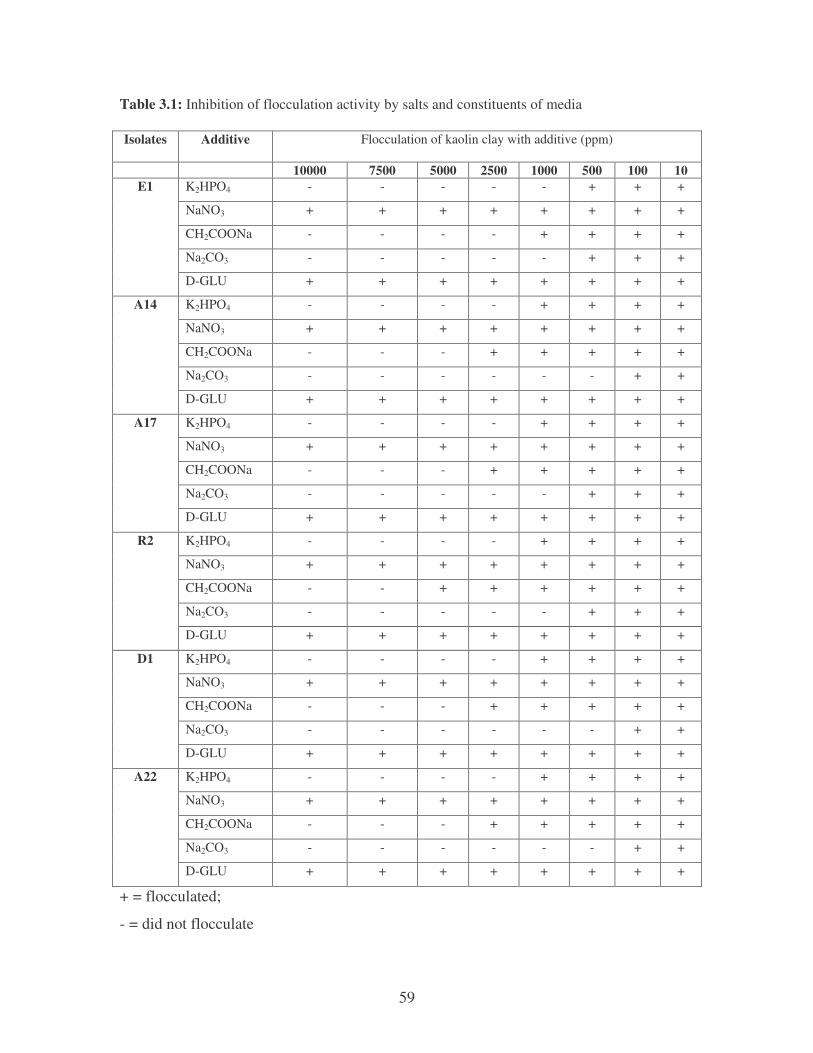
59
Table 3.1: Inhibition of flocculation activity by salts and constituents of media Isolates Additive Flocculation of kaolin clay with additive (ppm)
10000 7500 5000 2500 1000 500 100 10
K2HPO4 - - - - - + + +
NaNO3 + + + + + + + +
CH2COONa - - - - + + + +
Na2CO3 - - - - - + + +
E1
D-GLU + + + + + + + +
K2HPO4 - - - - + + + +
NaNO3 + + + + + + + +
CH2COONa - - - + + + + +
Na2CO3 - - - - - - + +
A14
D-GLU + + + + + + + +
K2HPO4 - - - - + + + +
NaNO3 + + + + + + + +
CH2COONa - - - + + + + +
Na2CO3 - - - - - + + +
A17
D-GLU + + + + + + + +
K2HPO4 - - - - + + + +
NaNO3 + + + + + + + +
CH2COONa - - + + + + + +
Na2CO3 - - - - - + + +
R2
D-GLU + + + + + + + +
K2HPO4 - - - - + + + +
NaNO3 + + + + + + + +
CH2COONa - - - + + + + +
Na2CO3 - - - - - - + +
D1
D-GLU + + + + + + + +
K2HPO4 - - - - + + + +
NaNO3 + + + + + + + +
CH2COONa - - - + + + + +
Na2CO3 - - - - - - + +
A22
D-GLU + + + + + + + +
+ = flocculated;
- = did not flocculate
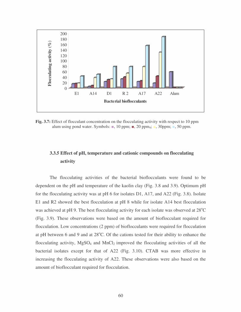
60
020406080
100120140160180200
Floc
cula
ting
activ
ity (%
)
E1 A14 D1 R 2 A17 A22 Alum
Bacterial bioflocculants
Fig. 3.7: Effect of flocculant concentration on the flocculating activity with respect to 10 ppm alum using pond water. Symbols: �, 10 ppm; �, 20 ppm4; �, 30ppm; �, 50 ppm.
3.3.5 Effect of pH, temperature and cationic compounds on flocculating
activity
The flocculating activities of the bacterial bioflocculants were found to be
dependent on the pH and temperature of the kaolin clay (Fig. 3.8 and 3.9). Optimum pH
for the flocculating activity was at pH 6 for isolates D1, A17, and A22 (Fig. 3.8). Isolate
E1 and R2 showed the best flocculation at pH 8 while for isolate A14 best flocculation
was achieved at pH 9. The best flocculating activity for each isolate was observed at 28oC
(Fig. 3.9). These observations were based on the amount of bioflocculant required for
flocculation. Low concentrations (2 ppm) of bioflocculants were required for flocculation
at pH between 6 and 9 and at 28oC. Of the cations tested for their ability to enhance the
flocculating activity, MgSO4 and MnCl2 improved the flocculating activities of all the
bacterial isolates except for that of A22 (Fig. 3.10). CTAB was more effective in
increasing the flocculating activity of A22. These observations were also based on the
amount of bioflocculant required for flocculation.
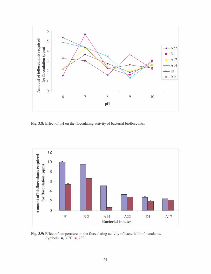
61
0
1
2
3
4
5
6
6 7 8 9 10
pH
Am
ount
of i
oflo
ccul
ants
req
uire
ddfo
r flo
ccul
atio
n (p
pm) A22
D1A17A14E1R 2
Fig. 3.8: Effect of pH on the flocculating activity of bacterial biofloccunts.
0
2
4
6
8
10
12
E1 R 2 A14 A22 D1 A17Bacterial isolates
Am
ount
of b
ioflo
ccul
ants
req
uire
dd
for
flocc
ulat
ion
(ppm
)
Fig. 3.9: Effect of temperature on the flocculating activity of bacterial bioflocculants. Symbols: �, 37oC; �, 28oC.
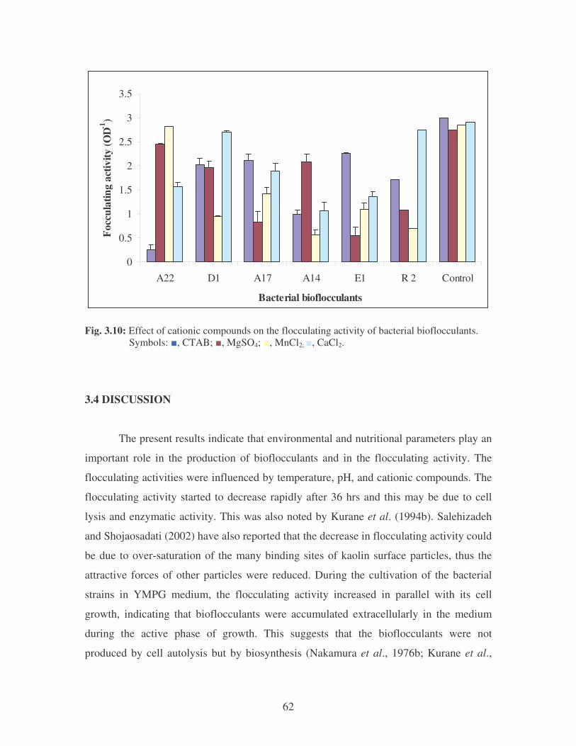
62
0
0.5
1
1.5
2
2.5
3
3.5
A22 D1 A17 A14 E1 R 2 Control
Bacterial bioflocculants
Focc
ulat
ing
activ
ity (O
D-1)
Fig. 3.10: Effect of cationic compounds on the flocculating activity of bacterial bioflocculants. Symbols: �, CTAB; �, MgSO4; �, MnCl2; �, CaCl2.
3.4 DISCUSSION
The present results indicate that environmental and nutritional parameters play an
important role in the production of bioflocculants and in the flocculating activity. The
flocculating activities were influenced by temperature, pH, and cationic compounds. The
flocculating activity started to decrease rapidly after 36 hrs and this may be due to cell
lysis and enzymatic activity. This was also noted by Kurane et al. (1994b). Salehizadeh
and Shojaosadati (2002) have also reported that the decrease in flocculating activity could
be due to over-saturation of the many binding sites of kaolin surface particles, thus the
attractive forces of other particles were reduced. During the cultivation of the bacterial
strains in YMPG medium, the flocculating activity increased in parallel with its cell
growth, indicating that bioflocculants were accumulated extracellularly in the medium
during the active phase of growth. This suggests that the bioflocculants were not
produced by cell autolysis but by biosynthesis (Nakamura et al., 1976b; Kurane et al.,

63
1986b). The correlation between cell growth and secretion of extracellular biopolymeric
flocculants (EBFs) was originally reported by McKinney (1956).
Fujita et al. (2000) noted that the biological flocculation does not occur until the
microorganisms have entered into an endogenous phase. In this study bioflocculant
production remained constant after 84 hrs. This could be because carbon and nitrogen
sources in the medium were used up. In a study done by Norberg and Enfors (1982) on Z.
ramigera, the flocculant production ended after 90 hrs in the stationary phase. The
production of the flocculant by S. griseus was not growth-related. For S. griseus, the
flocculating activity increased rapidly with increasing time of cultivation after the third
day and reached a maximum value after 4 days (Shimofuruya et al., 1996).
Flavobacterium sp. showed flocculating activity at the end of exponential growth phase
and the beginning of the stationary phase (Hantula and Bamford, 1991a; b). In contrast to
those observations, the flocculant production in R. erythropolis (Kurane et al., 1991), A.
sojae (Nakamura et al., 1976b), Zoogloea MP6 (Unz and Farrah, 1976), and Alcaligenes
latus (Kurane and Nohata, 1991) have been found to be parallel to cell growth. This
observation is consistent with the findings of the present study where flocculant
production, flocculating activity and removal of kaolin clay were parallel to the cell
growth.
It is clear that with an increase in flocculant concentration the percentage removal
of kaolin clay increases and then a decrease in kaolin removal was observed with a
further increase in concentration level. This may be because an optimum amount of
flocculants in the suspension causes a larger amount of kaolin particles to aggregate and
settle. However, according to Chan and Chiang (1995) the amount exceeding the
optimum concentration of flocculants is known to cause the aggregated particle to
redisperse and would also disturb particle settling. This behaviour could also be caused
by an increase in the repulsive energy between the flocculants and kaolin in solution,
which causes hindrance in floc formation (Mishra et al., 2004). The basal surfaces of
kaolinite are believed to carry a constant structural charge due to the isomorphous
substitution of Si4+ by Al3+, whereas the charge on the edges are due to the
64
protonation/deprotonation of exposed hydroxyl groups and depend on the pH of the
solution. Johnson et al. (2000) suggested that the charge on the basal surface is pH
dependent. It has been shown that an edge surface which should carry a positive double
layer in acid solution, and a negative double layer in alkaline solution, with a point of
zero charge (PZC) in the region of pH 7, dependent on the particular kaolinite crystal
structure (Hu and Liu, 2003).
In this study, all the bacterial bioflocculants were effective in flocculating C.
hystolyticum, S. cerevisiae, and A. faecalis. Other bacterial cultures flocculated but to a
lesser extent. Flocculation in S. cerevisiae is due to the presence of dominant flocculation
genes FLO1 and FLO2 and a recessive gene flo3 (Lewis et al., 1976 – cited by Jin and
Speers, 1998). The European Brewery Convention (EBC) suggested that the aggregation
of yeast cells into flocs may be due to either non-separation of cells after budding or
coalescence of single cells into clumps (EBC Microbiologica, 1981 – cited by Jin and
Speers, 1998). Yeast flocculation has been defined as the phenomenon wherein yeast
cells adhere in clumps and sediment rapidly from the medium in which they are
suspended (Stewart et al., 1976 – cited by Jin and Speers, 1998). The responsible bonding
has been proved to involve lectin-like protein-carbohydrate recognition and interaction
(Jin and Speers, 1998). Bacterial bioflocculants flocculated 76 bacterial species in a floc
and caused 15 species to float in a floc. The remaining 9 species were flocculated little if
at all. Bacteria that precipitated included P. aeruginosa IFO 3924, P. fluorescens S272
and E. coli K12 (Nakata and Kurane, 1999).
The application of bioflocculants for the removal of suspended fine particles and
organic matter from raw water was examined in comparison with a conventional
coagulant agent, alum. The results indicated that the bioflocculants were efficient for the
removal of these particles and organic matter. Furthermore, the bioflocculants produced
similar results, as did the use of alum, but at a slightly higher dosage. Fujita et al. (2000)
indicated that the flocculation of kaolin by the Citrobacter sp. TKF04 was comparable to
or slightly lower than that of PAA (polyacrylamide) and much higher than that of PAC
(polyaluminum chloride).
65
Of the various cations tested on the flocculating activity of the bioflocculants the
most effective was Mn2+ and Mg2+. The flocculating activity was not enhanced by the
addition of Ca2+. Shimofuruya et al. (1996) reported that a high concentration of Ca2+ led
to the decrease in flocculating activity. The divalent cations accelerate the initial
adsorption of the biopolymer on kaolin particles by decreasing the negative electrical
charge of kaolin particles and the biopolymer flocculants (Salehizadeh and Shojaosadati,
2002). Divalent cations have a significant effect on the coagulation of natural colloidal
particles. Black et al. (1966) suggested that Mg2+ affects the stability of anionic polymer-
clay. Three mechanisms are possible: firstly, divalent cations compress the double layer
of colloid; secondly, the repulsive forces between polymers and clay particles are reduced
by the cations that enhance adsorption of the polymer on the clay particle, and finally the
range of repulsive barrier between adsorbed anionic polymers is probably reduced by
Mg2+. This is reasonably strong evidence that indicates that divalent ions are necessary
for polymers to flocculate negative colloids. In this study, anions such as carbonic and
phosphate ions prevented proper flocculation by forming weak or loose structures often
decreasing the floc size (Faust and Aly, 1998) (Table 3.1).
The optimum pH for the flocculating activity was observed between pH 6 and 9
(Fig. 3.8). In contrast to the finding of the current study Kurane et al. (1994a) reported
that flocculation did not decrease with an alkaline pH of up to 10. The possible reason for
this observation could be that different genera and species of bacteria was used in this
study. Also, these bacteria were isolated from different environments. With respect to
temperature the optimum flocculating activity was observed at 28oC (Fig. 3.9). Yokoi et
al. (1996a) showed that the effective flocculation of kaolin suspension by Bacillus
licheniformis occurred between the temperatures of 4-90oC. Lian et al. (2007) found that
the flocculation ratio varies from approximately 85% to 89% in the temperature range of
23 to 70oC, and only begins to decrease noticeably with further temperature increase from
70 to 90 oC. The slight increase in the flocculation ratio from 23 to 40oC may be
explained by the higher random motion of the flocculant molecules, and hence, higher
collision frequency with kaolin particles. Thus, it appears that temperature has little
impact on the physical and chemical properties of the flocculant molecules in the
66
temperature range of 23–70oC. Fujita et al. (2000) indicated that efficient kaolin removal
by the bioflocculant produced by Citrobacter sp. TKF04, could be performed in a pH
range of 2-8 and temperature range of 3-95oC and it could flocculate a variety of organic
and inorganic particles.
In conclusion, the bioflocculants produced by these bacterial strains have a
satisfactory level of flocculating activity. These results suggest that these bioflocculants
can be successfully applied for the clarification of river water or wastewaters under
various environmental conditions. Overall, it can be concluded that these bioflocculants
exhibit flocculating activity comparable or superior to that of existing inorganic
flocculants (alum).
67
CHAPTER FOUR
MICROBIAL DECOLOURIZATION OF EFFLUENTS CONTAINING
TEXTILE-DYES
4.1 INTRODUCTION
The use of synthetic chemical dyes in various industrial processes has increased
considerably over the last few years. Some areas where these chemicals are frequently
used are paper and pulp manufacturing, plastics, dyeing of cloth, leather treatment and
printing (Aksu, 2005). Industrial wastewater containing such dyes is generally discarded
as effluents. Since some of these dyes are toxic in nature, their presence in from the
industrial effluents is a major environmental problem, because they are recalcitrant to
microbial degradation (Pagga and Brown, 1986). The wastewater, which is highly
coloured, can block the penetration of sunlight and oxygen, which are essential for the
survival of various aquatic forms. Moreover, the dye solution can also undergo anaerobic
degradation to form potentially carcinogenic compounds, which can end up in the food
chain. Many approaches, including physical and/or chemical processes have been used in
the treatment of dye containing industrial wastewater; however, such methods are often
very costly (Nigam et al., 1996; Rauf et al., 2006).
In recent times, industries have been faced with more stringent effluent
regulations. For instance, the textile, food, and pharmaceutical industry are required to
lower the colour content in their wastewater (Pinheiro et al., 2004). Flocculation and
precipitation processes have proved to be an effective procedure for the decolourization
of such effluents (Mishra and Bajpai, 2005). Physical-chemical flocculation with metal
hydroxides assisted by polymer flocculants is the most widely used method of treatment
for coloured effluents (Choy et al., 2001). However, other alternatives such as powdered
activated carbon and activated bentonites can also be used (Pala and Tokat, 2002; Yavuz
and Aydin, 2002). The major disadvantages of this technique are the large amount of
68
sludge, which has to be buried, and the low efficiency with respect to some dyes (Pearce
et al., 2003).
Colour removal is also usually effective and fairly rapid using ozone. However,
not all the methods employed give satisfactory results especially for some dispersed dyes.
Therefore, new flocculation mechanisms have been attracting attention (Petzold et al.,
2003a). Salts alone or in combination with polymers were used for the neutralization of
charged particles to obtain coagulation. The flocculation mechanism depends on the
properties of polymers, especially the type of charge (negative, positive or uncharged),
the charge density, and the molecular weight. Highly charged polyelectrolytes with low
molecular weight can cause flocculation by interaction between differently charged
regions of the particles (patch flocculation); whereas polymers of very high molecular
weight (several millions) can cause bridging. The combined use of cationic flocculant
and anionic polyelectrolytes of high molecular weight (step by step) is successful because
the two flocculation mechanisms can be combined: at first “patching” is obtained by the
highly charged polycation and, in a second step, bridging is caused by the high molecular
weight polyanion. This mechanism works very well for small particles, such as clay or
cellulose-clay mixtures (Petzold et al., 2003b; Petzold et al., 2004).
Another, more practicable method is the application of pre-mixed polyelectrolyte
complexes made by the interaction of aqueous solutions of polycation and polyanion that
was first described for clay (Petzold et al., 1998). However, because dye molecules or
their aggregates are incomparably smaller than such inorganic particles and, in some
cases, they are also uncharged, it is necessary to apply other flocculation principles, for
instance the inclusion of dye within complexes. Such complex particles, the so-called
particle forming flocculants, are able to bind disperse−dyes effectively over large
distances due to their size and structure. Complex particles with hydrophobic parts and
positive or negative charge are able to bind the dye via hydrophobic as well as
electrostatic interaction forces (Buchhammer et al., 2001).
69
Textile industries consume substantial volumes of water and chemicals for wet
processing of textiles. These chemicals are used for desiring, scouring, bleaching, dyeing,
printing, and finishing. They range from inorganic compounds and elements to polymers
and organic products. There are more than 8 000 chemical products associated with the
dyeing process listed in the Colour Index (Society of Dyers and Colourists, 1976 − cited
by Banat et al., 1996). These dyes include several structural varieties of dyes, such as
acidic, reactive, basic, disperse, azo, diazo, anthraquinone-based and metal-complex
dyes. The only aspect in common is their ability to absorb light in the visible region
(Song et al., 2006).
The removal of colour from wastewaters is often more important than the removal
of the soluble colourless organic substances, which usually contribute the major fraction
of the biochemical oxygen demand (BOD). Methods for the removal of BOD from most
effluents are fairly well established; dyes, however, are more difficult to treat because of
their synthetic origin and mainly complex aromatic molecular structures. Such structures
are often synthesized to resist fading on exposure to sweat, soap, water, light or oxidizing
agents (Aksu, 2005; Khan and Husain 2007) and this renders them more stable and less
amenable to biodegradation (Fewson, 1988; Seshadri et al., 1994).
Dyes with simple structures and low molecular weights exhibit higher rates of
colour removal, whereas colour removal is more difficult with highly substituted, high
molecular weight dyes (Sani and Banerjee, 1999). The dye removal rates are influenced
by changes in electron density in the region of the azo group. The substitution of electron
withdrawing groups (–SO3H,–SO2NH2) in the para position of the phenyl ring, relative to
the azo bond, causes an increase in the reduction rate (Yilmaz et al., 2007). Nigam et al.
(1996) established that azo compounds with a hydroxyl group or with an amino group are
more likely to be removed than are those with a methyl, methoxy, sulpho or nitro groups.
Colour removal is also related to the number of azo bonds in the dye molecule. The
colour of monoazo dyes is removed faster than the colour of diazo or triazo dyes (Nigam
et al., 1996).
70
Government legislation is becoming more stringent in most developed countries
regarding the removal of dyes from industrial effluents, which is in turn becoming an
increasing problem for the textile industries. Environmental-protection agencies in
Europe are promoting prevention of transferral of pollution problems from one part of the
environment to another. This means that for most textile industries, developing on-site or
in-plant facilities to treat their own effluents before discharge is fast approaching
actuality. Recently, state and federal agencies in the USA have been requiring lower
effluent colour limits (< 200 units of American Dye Manufacturers Institute, ADMI)
(McCurdy et al., 1992).
Interest in the pollution potential of textile dyes has been primarily prompted by
concern over their possible toxicity and carcinogenicity. This is mainly because many
dyes are made from known carcinogens, such as benzidine and other aromatic
compounds, all of which might be reformed because of microbial metabolism (Khan and
Husain 2007). It has been shown that azo and nitro compounds are reduced in sediments
(Weber and Wolfe, 1987) and in the intestinal environment (Sirianuntapiboon and
Srisornsak, 2007), resulting in the regeneration of the parent toxic amines.
Anthraquinone-based dyes are most resistant to degradation due to their fused aromatic
structures, which remain coloured for long periods. Basic dyes have high brilliance and
therefore higher colour intensity, making them more difficult to decolourize, while metal-
based complex dyes, such as chromium-based dyes, can lead to the release of chromium,
which is carcinogenic in nature, into water supplies. Some disperse dyes have also been
shown to have a tendency to bio-accumulate (Baughman and Perenich, 1988) and heavy-
metal ions from textile effluents have also been reported at high concentrations in both
algae and higher plants exposed to such effluents (Srivastava and Prakash, 1991).
The lack of data on the properties of many dyes has been the main problem in
assessing broad classes of dyes to identify common characteristics. Although dyes
constitute only a small portion of the total volume of waste discharge in textile
processing, these compounds are not readily removed by typical microbial-based waste-
treatment processes (Li et al., 2007). Furthermore, dyes can be detrimental to the

71
microbial population present in such treatment works and may lead to decreased
efficiency or treatment failure in such plants (Ogawa et al., 1988). Similar adverse effects
have also been detected for aquatic microbial populations and the aquatic environment in
general (Pearce et al., 2003) or for laboratory cultures exposed to such dyes (Ogawa et
al., 1989).
Azo dyes, which are difficult to degrade biologically and chemically, constitute the
largest group of colorants used in industry. They are commonly found in considerable
amounts in wastewater released by dye-house effluents. Their presence in dyeing and
production of dye wastewater causes high concentration of dissolved organic matter and
deep colour. If these wastewaters are not treated properly, they can flow into lakes, rivers,
and seas through public sewage and then contaminate the environments where people
live. It is reported that azo dyes themselves are not toxic; however, under anaerobic
conditions azo dyes are cleaved by microorganisms to form potentially carcinogenic
aromatic amines (Li et al., 2007). Since many textile plants have rural locations and
municipal treatment costs are increasing, both industries and scientists are becoming
compelled to search for innovative novel treatments and technologies directed
particularly towards the decolourization of dyes in effluents. Dyes usually have a very
low rate of removal ratio for BOD to COD (BOD/COD less than 0.1). Biological
methods, being cheap and simple to use, have been the focus of recent studies on dye
degradation and decolourization (Sirianuntapiboon and Srisornsak, 2007). Therefore, the
objective of this chapter was to evaluate the ability of the bacterial bioflocculants to
remove dyes and chemicals from the textile industrial effluents.
4.2 MATERIALS AND METHODS
4.2.1 Textile dyes used in this study
The three types of dispersible dyes selected for use in this study were whale,
medi-blue, fawn and a mixture of dyes (see Section 4.2.2). The chemical properties of
these dyes are described in Table 4.1.
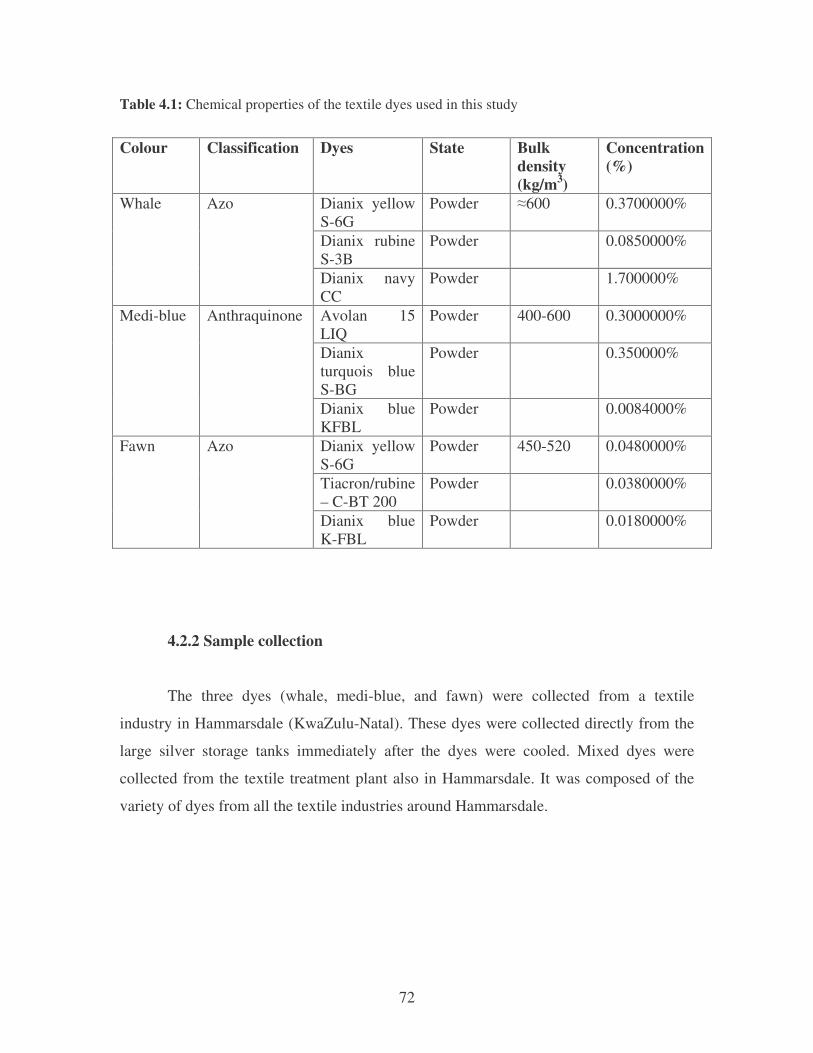
72
Table 4.1: Chemical properties of the textile dyes used in this study
Colour Classification Dyes State Bulk
density (kg/m3)
Concentration (%)
Dianix yellow S-6G
Powder �600 0.3700000%
Dianix rubine S-3B
Powder 0.0850000%
Whale Azo
Dianix navy CC
Powder 1.700000%
Avolan 15 LIQ
Powder 400-600 0.3000000%
Dianix turquois blue S-BG
Powder 0.350000%
Medi-blue Anthraquinone
Dianix blue KFBL
Powder 0.0084000%
Dianix yellow S-6G
Powder 450-520 0.0480000%
Tiacron/rubine – C-BT 200
Powder 0.0380000%
Fawn Azo
Dianix blue K-FBL
Powder 0.0180000%
4.2.2 Sample collection
The three dyes (whale, medi-blue, and fawn) were collected from a textile
industry in Hammarsdale (KwaZulu-Natal). These dyes were collected directly from the
large silver storage tanks immediately after the dyes were cooled. Mixed dyes were
collected from the textile treatment plant also in Hammarsdale. It was composed of the
variety of dyes from all the textile industries around Hammarsdale.
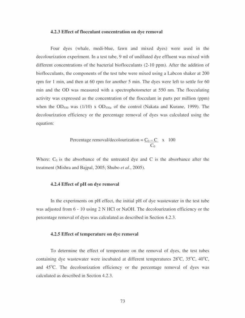
73
4.2.3 Effect of flocculant concentration on dye removal
Four dyes (whale, medi-blue, fawn and mixed dyes) were used in the
decolourization experiment. In a test tube, 9 ml of undiluted dye effluent was mixed with
different concentrations of the bacterial bioflocculants (2-10 ppm). After the addition of
bioflocculants, the components of the test tube were mixed using a Labcon shaker at 200
rpm for 1 min, and then at 60 rpm for another 5 min. The dyes were left to settle for 60
min and the OD was measured with a spectrophotometer at 550 nm. The flocculating
activity was expressed as the concentration of the flocculant in parts per million (ppm)
when the OD550 was (1/10) x OD550c of the control (Nakata and Kurane, 1999). The
decolourization efficiency or the percentage removal of dyes was calculated using the
equation:
Percentage removal/decolourization = C0 – C x 100 C0
Where: C0 is the absorbance of the untreated dye and C is the absorbance after the
treatment (Mishra and Bajpal, 2005; Shubo et al., 2005).
4.2.4 Effect of pH on dye removal
In the experiments on pH effect, the initial pH of dye wastewater in the test tube
was adjusted from 6 - 10 using 2 N HCl or NaOH. The decolourization efficiency or the
percentage removal of dyes was calculated as described in Section 4.2.3.
4.2.5 Effect of temperature on dye removal
To determine the effect of temperature on the removal of dyes, the test tubes
containing dye wastewater were incubated at different temperatures 28oC, 35oC, 40oC,
and 45oC. The decolourization efficiency or the percentage removal of dyes was
calculated as described in Section 4.2.3.
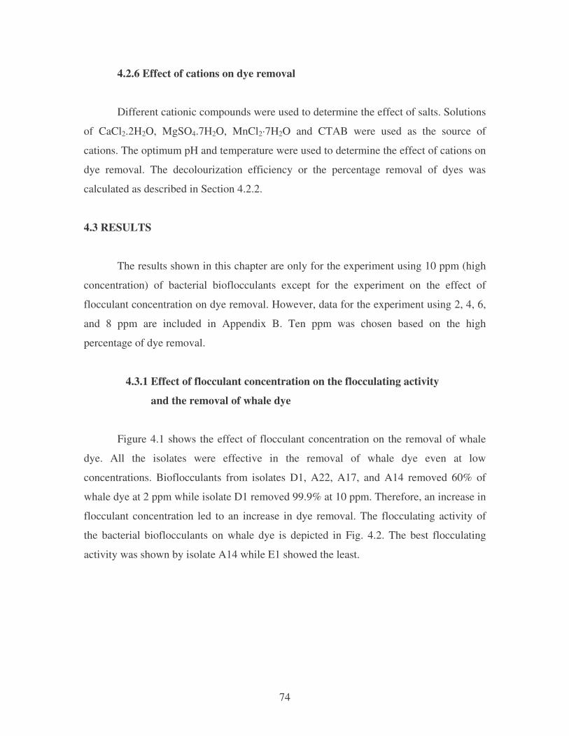
74
4.2.6 Effect of cations on dye removal
Different cationic compounds were used to determine the effect of salts. Solutions
of CaCl2.2H2O, MgSO4.7H2O, MnCl2·7H2O and CTAB were used as the source of
cations. The optimum pH and temperature were used to determine the effect of cations on
dye removal. The decolourization efficiency or the percentage removal of dyes was
calculated as described in Section 4.2.2.
4.3 RESULTS
The results shown in this chapter are only for the experiment using 10 ppm (high
concentration) of bacterial bioflocculants except for the experiment on the effect of
flocculant concentration on dye removal. However, data for the experiment using 2, 4, 6,
and 8 ppm are included in Appendix B. Ten ppm was chosen based on the high
percentage of dye removal.
4.3.1 Effect of flocculant concentration on the flocculating activity
and the removal of whale dye
Figure 4.1 shows the effect of flocculant concentration on the removal of whale
dye. All the isolates were effective in the removal of whale dye even at low
concentrations. Bioflocculants from isolates D1, A22, A17, and A14 removed 60% of
whale dye at 2 ppm while isolate D1 removed 99.9% at 10 ppm. Therefore, an increase in
flocculant concentration led to an increase in dye removal. The flocculating activity of
the bacterial bioflocculants on whale dye is depicted in Fig. 4.2. The best flocculating
activity was shown by isolate A14 while E1 showed the least.
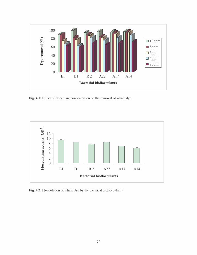
75
0
20
40
60
80
100
Dye
rem
oval
(%)
E1 D1 R 2 A22 A17 A14
Bacterial bioflocculants
10ppm8ppm6ppm4ppm2ppm
Fig. 4.1: Effect of flocculant concentration on the removal of whale dye.
02468
1012
E1 D1 R 2 A22 A17 A14
Bacterial bioflocculants
Floc
cula
ting
activ
ity (O
D-1)
Fig. 4.2: Flocculation of whale dye by the bacterial bioflocculants.
76
4.3.2 Effect of pH, temperature, and cations on the removal of whale dye
pH is the most important parameter affecting the removal of various dyes from
textile industries. The effect of pH on the removal of whale dye at 10 ppm flocculant
concentration is shown in Fig. 4.3. The optimum pH for the removal of whale dye was
pH 7 for all the isolates. At pH 6, 8, 9, and 10 there was a slight decrease in the removal
of whale dye. At pH 10, 70% of whale dye was removed by isolates E1, R2, A17 and
A14 while at pH 7, 99% of the dye was removed by all the bacterial isolates.
The optimum temperature for the removal of whale dye was 35oC for all the
isolates where 99% of the dye was removed (Fig. 4.4). At 45oC, there was a decrease in
the percentage removal of whale dye. This is shown clearly by isolates E1 and A17,
where 58% and 62% of the dye was removed, respectively. The effect of cations on the
removal of whale dye is depicted in Fig. 4.5. The most effective cation for the removal of
whale dye was MnCl2, followed by MgSO4 and CaCl2. Ninety-nine percent of whale dye
was removed upon the addition of MnCl2. CTAB was the least effective of all the cations
tested.
0
20
40
60
80
100
E1 D1 R 2 A22 A17 A14
Bacterial bioflocculants
Dye
rem
oval
(%) 6
78910
Fig. 4.3: Effect of pH on the removal of whale dye at 10 ppm.
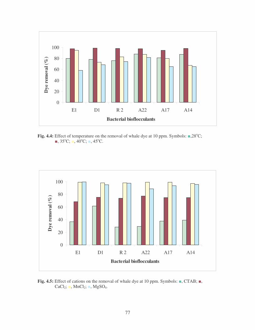
77
0
20
40
60
80
100
E1 D1 R 2 A22 A17 A14
Bacterial bioflocculants
Dye
rem
oval
(%)
Fig. 4.4: Effect of temperature on the removal of whale dye at 10 ppm. Symbols: �,28oC; �, 35oC; �, 40oC; �, 45oC.
0
20
40
60
80
100
E1 D1 R 2 A22 A17 A14
Bacterial bioflocculants
Dye
rem
oval
(%)
Fig. 4.5: Effect of cations on the removal of whale dye at 10 ppm. Symbols: �, CTAB; �, CaCl2; �, MnCl2; �, MgSO4.
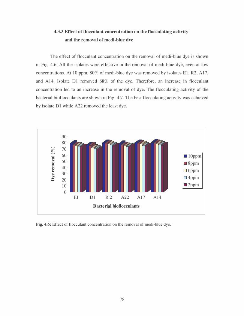
78
4.3.3 Effect of flocculant concentration on the flocculating activity
and the removal of medi-blue dye
The effect of flocculant concentration on the removal of medi-blue dye is shown
in Fig. 4.6. All the isolates were effective in the removal of medi-blue dye, even at low
concentrations. At 10 ppm, 80% of medi-blue dye was removed by isolates E1, R2, A17,
and A14. Isolate D1 removed 68% of the dye. Therefore, an increase in flocculant
concentration led to an increase in the removal of dye. The flocculating activity of the
bacterial bioflocculants are shown in Fig. 4.7. The best flocculating activity was achieved
by isolate D1 while A22 removed the least dye.
0102030405060708090
Dye
rem
oval
(%)
E1 D1 R 2 A22 A17 A14
Bacterial bioflocculants
10ppm8ppm6ppm4ppm2ppm
Fig. 4.6: Effect of flocculant concentration on the removal of medi-blue dye.
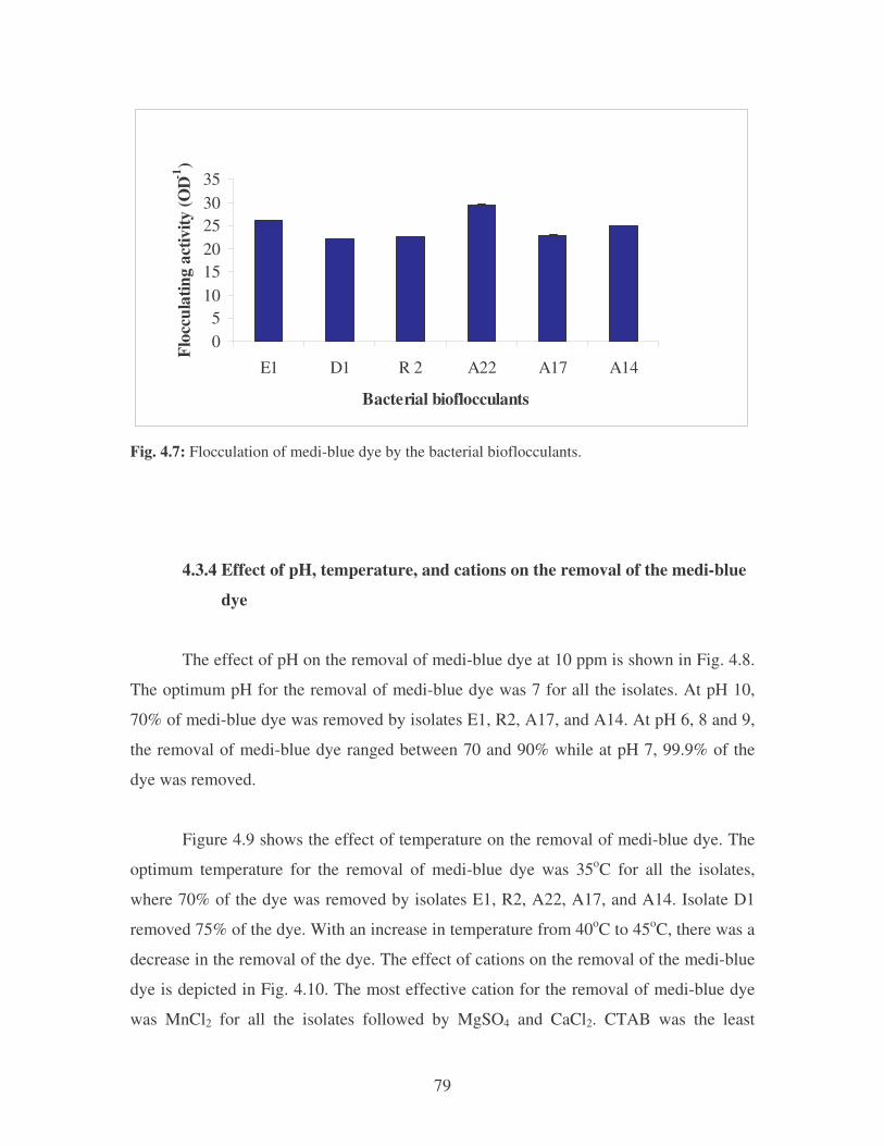
79
05
101520253035
E1 D1 R 2 A22 A17 A14
Bacterial bioflocculants
Floc
cula
ting
activ
ity (O
D-1)
Fig. 4.7: Flocculation of medi-blue dye by the bacterial bioflocculants.
4.3.4 Effect of pH, temperature, and cations on the removal of the medi-blue
dye
The effect of pH on the removal of medi-blue dye at 10 ppm is shown in Fig. 4.8.
The optimum pH for the removal of medi-blue dye was 7 for all the isolates. At pH 10,
70% of medi-blue dye was removed by isolates E1, R2, A17, and A14. At pH 6, 8 and 9,
the removal of medi-blue dye ranged between 70 and 90% while at pH 7, 99.9% of the
dye was removed.
Figure 4.9 shows the effect of temperature on the removal of medi-blue dye. The
optimum temperature for the removal of medi-blue dye was 35oC for all the isolates,
where 70% of the dye was removed by isolates E1, R2, A22, A17, and A14. Isolate D1
removed 75% of the dye. With an increase in temperature from 40oC to 45oC, there was a
decrease in the removal of the dye. The effect of cations on the removal of the medi-blue
dye is depicted in Fig. 4.10. The most effective cation for the removal of medi-blue dye
was MnCl2 for all the isolates followed by MgSO4 and CaCl2. CTAB was the least
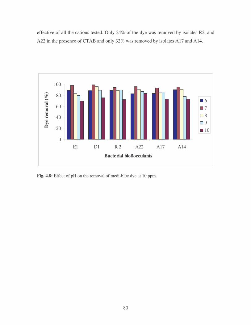
80
effective of all the cations tested. Only 24% of the dye was removed by isolates R2, and
A22 in the presence of CTAB and only 32% was removed by isolates A17 and A14.
0
20
40
60
80
100
E1 D1 R 2 A22 A17 A14
Bacterial bioflocculants
Dye
rem
oval
(%)
678910
Fig. 4.8: Effect of pH on the removal of medi-blue dye at 10 ppm.
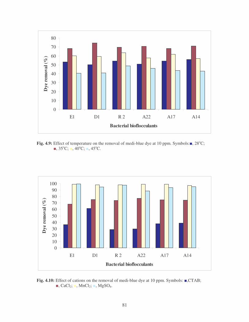
81
0
10
20
30
40
50
60
70
80
E1 D1 R 2 A22 A17 A14
Bacterial bioflocculants
Dye
rem
oval
(%)
Fig. 4.9: Effect of temperature on the removal of medi-blue dye at 10 ppm. Symbols:�, 28oC; �, 35oC; �, 40oC; �, 45oC.
0102030405060708090
100
E1 D1 R 2 A22 A17 A14
Bacterial bioflocculants
Dye
rem
oval
(%)
Fig. 4.10: Effect of cations on the removal of medi-blue dye at 10 ppm. Symbols: �,CTAB; �, CaCl2; �, MnCl2; �, MgSO4.

82
4.3.5 Effect of flocculant concentration on the flocculating activity
and the removal of fawn dye
The effect of flocculant concentration on the removal of fawn dye is shown in
Fig. 4.11. Isolate D1 showed the best removal at 10 ppm where 99% of fawn dye was
removed followed by isolate E1 where 80% of the dye was removed at 10 ppm. At 2
ppm, the removal of the dye by isolates D1 and E1 were 90% and 70%, respectively.
Only 50% of fawn dye was removed by isolate R2 at 10 ppm. The removal of fawn dye
by the isolates A22, A17, and A14 was less effective even with an increase in the
flocculant concentration. The flocculating activity of the bacterial bioflocculants are
depicted in Fig. 4.12. Isolate D1 showed the best flocculating activity while isolate A17
showed the least amount of activity. The flocculating activities of isolates E1, R2, A14,
and A22 ranged between 10 – 50 OD-1.
0
20
40
60
80
100
Dye
rem
oval
(%)
E1 D1 R 2 A22 A17 A14
Bacterial bioflocculants
10ppm8ppm6ppm4ppm2ppm
Fig. 4.11: Effect of flocculant concentration on the removal of fawn dye.
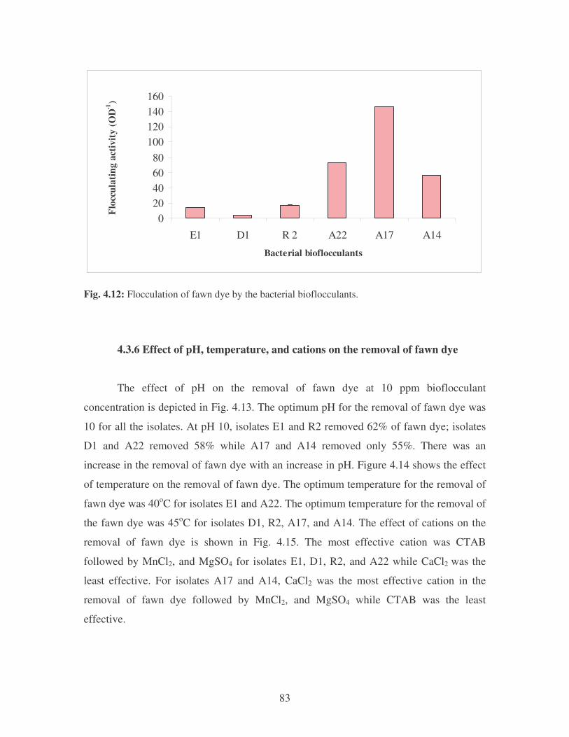
83
020406080
100120140160
E1 D1 R 2 A22 A17 A14
Bacterial bioflocculants
Floc
cula
ting
activ
ity (O
D-1)
Fig. 4.12: Flocculation of fawn dye by the bacterial bioflocculants.
4.3.6 Effect of pH, temperature, and cations on the removal of fawn dye
The effect of pH on the removal of fawn dye at 10 ppm bioflocculant
concentration is depicted in Fig. 4.13. The optimum pH for the removal of fawn dye was
10 for all the isolates. At pH 10, isolates E1 and R2 removed 62% of fawn dye; isolates
D1 and A22 removed 58% while A17 and A14 removed only 55%. There was an
increase in the removal of fawn dye with an increase in pH. Figure 4.14 shows the effect
of temperature on the removal of fawn dye. The optimum temperature for the removal of
fawn dye was 40oC for isolates E1 and A22. The optimum temperature for the removal of
the fawn dye was 45oC for isolates D1, R2, A17, and A14. The effect of cations on the
removal of fawn dye is shown in Fig. 4.15. The most effective cation was CTAB
followed by MnCl2, and MgSO4 for isolates E1, D1, R2, and A22 while CaCl2 was the
least effective. For isolates A17 and A14, CaCl2 was the most effective cation in the
removal of fawn dye followed by MnCl2, and MgSO4 while CTAB was the least
effective.
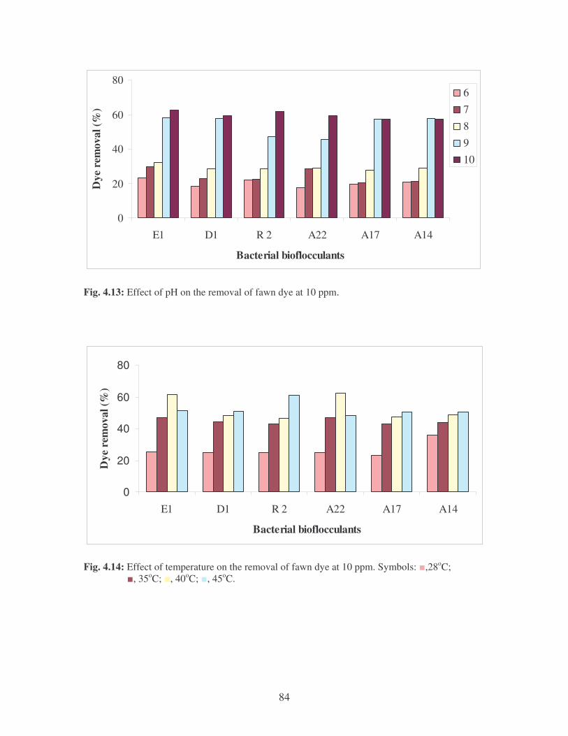
84
0
20
40
60
80
E1 D1 R 2 A22 A17 A14
Bacterial bioflocculants
Dye
rem
oval
(%)
678910
Fig. 4.13: Effect of pH on the removal of fawn dye at 10 ppm.
0
20
40
60
80
E1 D1 R 2 A22 A17 A14
Bacterial bioflocculants
Dye
rem
oval
(%)
Fig. 4.14: Effect of temperature on the removal of fawn dye at 10 ppm. Symbols: �,28oC; �, 35oC; �, 40oC; �, 45oC.
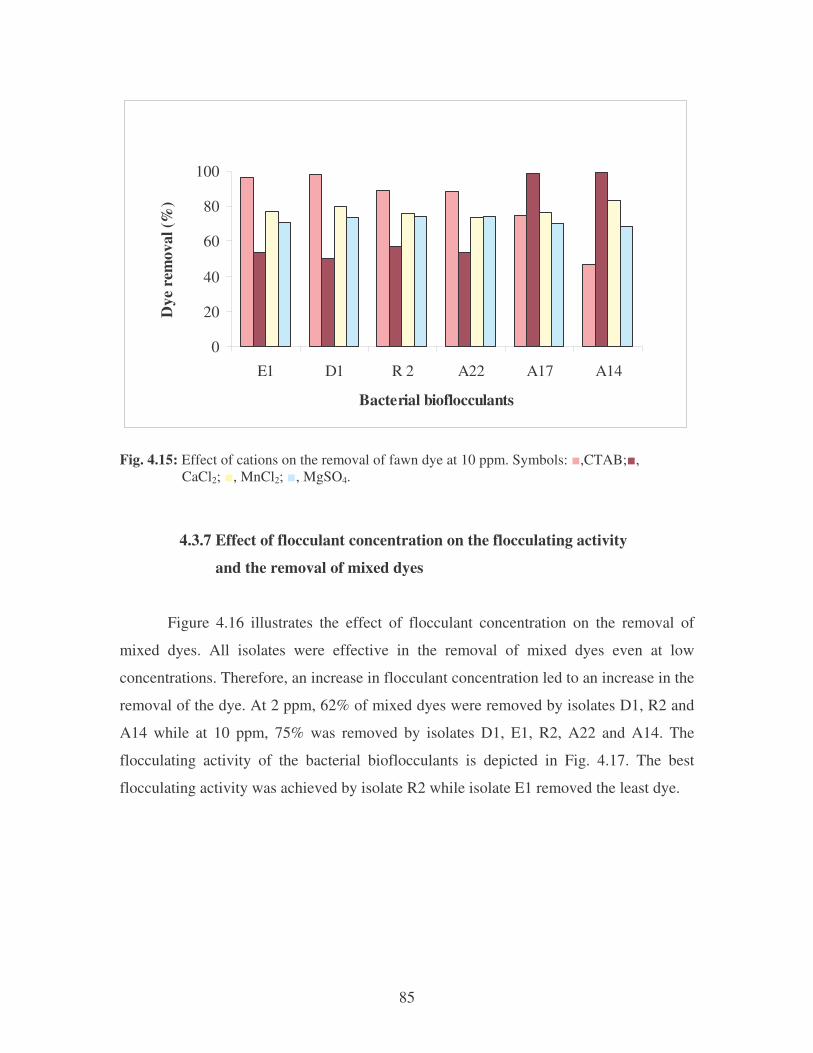
85
0
20
40
60
80
100
E1 D1 R 2 A22 A17 A14
Bacterial bioflocculants
Dye
rem
oval
(%)
Fig. 4.15: Effect of cations on the removal of fawn dye at 10 ppm. Symbols: �,CTAB;�, CaCl2; �, MnCl2; �, MgSO4.
4.3.7 Effect of flocculant concentration on the flocculating activity
and the removal of mixed dyes
Figure 4.16 illustrates the effect of flocculant concentration on the removal of
mixed dyes. All isolates were effective in the removal of mixed dyes even at low
concentrations. Therefore, an increase in flocculant concentration led to an increase in the
removal of the dye. At 2 ppm, 62% of mixed dyes were removed by isolates D1, R2 and
A14 while at 10 ppm, 75% was removed by isolates D1, E1, R2, A22 and A14. The
flocculating activity of the bacterial bioflocculants is depicted in Fig. 4.17. The best
flocculating activity was achieved by isolate R2 while isolate E1 removed the least dye.
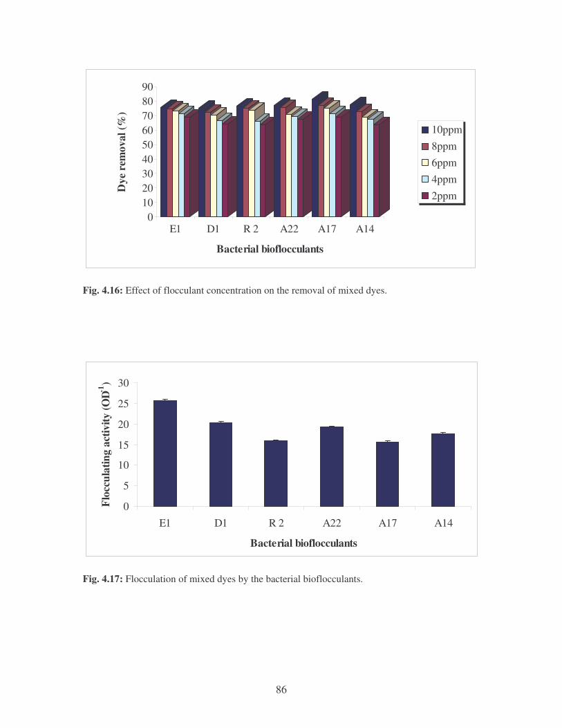
86
0102030405060708090
Dye
rem
oval
(%)
E1 D1 R 2 A22 A17 A14
Bacterial bioflocculants
10ppm8ppm6ppm4ppm2ppm
Fig. 4.16: Effect of flocculant concentration on the removal of mixed dyes.
0
5
10
15
20
25
30
E1 D1 R 2 A22 A17 A14
Bacterial bioflocculants
Floc
cula
ting
activ
ity (O
D-1)
Fig. 4.17: Flocculation of mixed dyes by the bacterial bioflocculants.
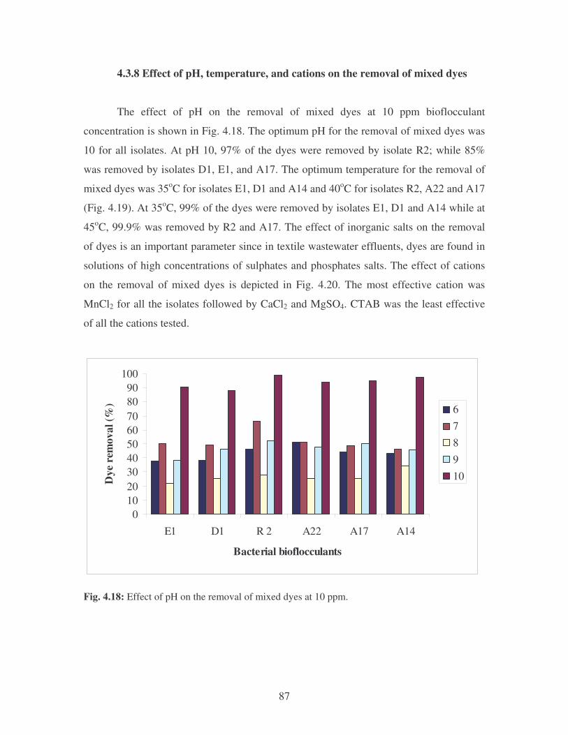
87
4.3.8 Effect of pH, temperature, and cations on the removal of mixed dyes
The effect of pH on the removal of mixed dyes at 10 ppm bioflocculant
concentration is shown in Fig. 4.18. The optimum pH for the removal of mixed dyes was
10 for all isolates. At pH 10, 97% of the dyes were removed by isolate R2; while 85%
was removed by isolates D1, E1, and A17. The optimum temperature for the removal of
mixed dyes was 35oC for isolates E1, D1 and A14 and 40oC for isolates R2, A22 and A17
(Fig. 4.19). At 35oC, 99% of the dyes were removed by isolates E1, D1 and A14 while at
45oC, 99.9% was removed by R2 and A17. The effect of inorganic salts on the removal
of dyes is an important parameter since in textile wastewater effluents, dyes are found in
solutions of high concentrations of sulphates and phosphates salts. The effect of cations
on the removal of mixed dyes is depicted in Fig. 4.20. The most effective cation was
MnCl2 for all the isolates followed by CaCl2 and MgSO4. CTAB was the least effective
of all the cations tested.
0102030405060708090
100
E1 D1 R 2 A22 A17 A14
Bacterial bioflocculants
Dye
rem
oval
(%) 6
78910
Fig. 4.18: Effect of pH on the removal of mixed dyes at 10 ppm.
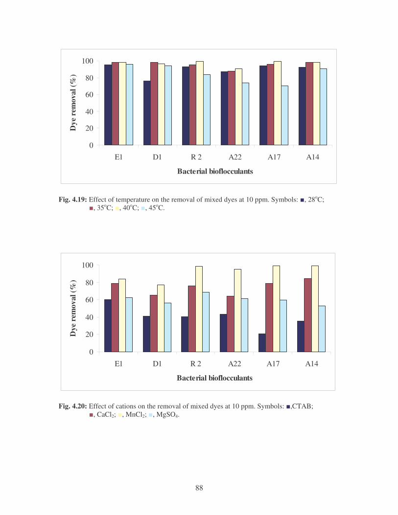
88
0
20
40
60
80
100
E1 D1 R 2 A22 A17 A14
Bacterial bioflocculants
Dye
rem
oval
(%)
Fig. 4.19: Effect of temperature on the removal of mixed dyes at 10 ppm. Symbols: �, 28oC; �, 35oC; �, 40oC; �, 45oC.
0
20
40
60
80
100
E1 D1 R 2 A22 A17 A14
Bacterial bioflocculants
Dye
rem
oval
(%)
Fig. 4.20: Effect of cations on the removal of mixed dyes at 10 ppm. Symbols: �,CTAB; �, CaCl2; �, MnCl2; �, MgSO4.
89
4.4 DISCUSSION
In this study, the effect of flocculant concentration on the removal of dyes was
investigated. The results have shown that the removal of all the dyes tested were directly
proportional to the flocculant concentration (Fig. 4.1; Fig. 4.6; Fig. 4.11; Fig. 4.16). The
flocculants cause aggregation of particles and cells by bridging and charge neutralization
(Salehizadeh and Sojaosadati, 2001). Bridging occurs if the flocculant extends from the
particle’s surface into the solution for a distance greater than the distance over which the
interparticle repulsion acts. In this case, the biopolymer can adsorb to other particles to
form flocs. This mechanism explains flocculation by neutral or like-charged
bioflocculants (Hantula and Bamford, 1991b; Levy et al., 1992). Shubo et al. (2005)
reported that higher decolourization of the dyes can be achieved by increasing the
concentration of the bioflocculants.
The flocculating capacity of the bioflocculants increased with an increase in
concentration and remained constant except for fawn dye where there was a slight
increase in flocculating capacity with an increase in flocculant concentration (Fig. 4.1;
Fig. 4.6; Fig. 4.11; Fig. 4.16). This observation may be due to a particle-polymer-particle
complex formation in which polymer serves as a bridge. To be effective in
destabilization, a polymer molecule must contain chemical groups, which can interact
with sites on the surface of the colloidal particle. When a polymer molecule comes into
contact with a colloidal particle, some of these groups adsorb at the particle surface,
leaving the remainder of the molecule extending out into the solution. If a second particle
with some vacant adsorption sites comes into contact with these extended segments,
attachment can occur. A particle-polymer-particle complex is thus formed in which
polymer serves as a bridge. If a second particle is not available, in time the extended
segments may eventually adsorb on other sites on the original particle, so that the
polymer is no longer capable of serving as a bridge (Salehizadeh and Sojaosadati, 2001;
Salehizadeh and Sojaosadati, 2002). Mishra and Bajpai (2005) indicated that there is
direct stoichiometric relationship between optimum polymer dosage and colloid
concentration, and restabilization due to overdosing can occur.

90
In this study, the optimum pH was observed at pH 7 for whale and medi-blue dyes
(Fig.4.3, Fig.4.8) while for fawn and mixed dyes it was observed at pH 10 (Fig. 4.13;
Fig.4.18). According to Willmott (1997), the optimum pH for colour removal is often at a
neutral pH value or a slightly alkaline pH value and the rate of colour removal tends to
decrease rapidly at strongly acid or strongly alkaline pH values. As a result, the coloured
wastewater is often buffered to enhance the colour removal performance. Colour removal
in the alkaline pH range is presumably due to adsorption onto hydroxide flocs. Biological
reduction of the azo bond of whale and fawn dye can result in an increase in the pH due
to the formation of aromatic amine metabolites, which are more basic than the original
azo compound (Willmott, 1997). Altering the pH within a range of 7.0 to 9.5 has very
little effect on the dye reduction process. Chang et al. (2001) found that the dye reduction
rate increased nearly 2.5-fold as the pH was raised from 5.0 to 7.0, while the rate became
insensitive to pH in the range of 7.0-9.5. This is in accordance with the results obtained in
this study. On the other hand Mittal and Gupta (1996), studied the effect of pH on the
biosorption of three cationic dyes, Orlamar Red BG, Orlamar Blue G and Orlamar Red
GTL by the fungus Fomitopsis carnea and their results showed that colour removal
decreased with decreasing pH due to repulsive forces between coloured dye cations in
solution and biosorbent surface charged positively at pH values lower than 3.0.
In many systems, the rate of colour removal increases with increasing
temperature, within a defined range that depends on the system (Chang et al., 2001). The
temperature required to produce the maximum rate of colour removal was found to range
between 35-45oC for all the textile dyes tested (Fig. 4.4; Fig. 4.9; Fig. 4.14; Fig. 4.19).
The results are consistent with a study done by Pearce et al. (2003) regarding the removal
of colour from textile wastewater using whole bacterial cells. The decline in colour
removal activity at higher temperatures can be attributed to the loss of cell viability
(Pearce et al., 2003). Aksu and Tezer (2000), also investigated the effect of temperature
on the biosorption of Remazol Black B reactive dye by Rhizopus arrhizus and their
results indicated that optimum adsorption temperature was 35oC and adsorption
decreased with further increasing temperature due to the decreased surface activity.
91
The addition of the divalent cations such as Mn2+, Mg2+, and Ca2+ enhanced both
the flocculating activity and the decolourization of the dyes (Fig. 4.5; Fig. 4.10; Fig. 4.15;
Fig. 4.20). Cations stimulate flocculating activity by neutralizing and stabilizing the
residual negative charge of functional groups and by forming bridges between particles.
The role of bivalent and trivalent cations is to increase the initial adsorption of
biopolymers on suspended particles by decreasing the negative charge on both the
polymer and the particle (Levy et al., 1992). The results are consistent with the findings
of Kurane et al. (1994b) who reported that divalent cations namely Mn2+, Mg2+, and Ca2+
bind to the bioflocculants and form complexes thus stimulating flocculation. Fujita et al.
(2000) and Yim et al. (2007) indicated that the flocculating activity of Citrobacter sp.
TKF04 and Gyrodinium impudicum KG03 was not enhanced by the addition of any
cations including Ca2+. Dyeing processes consume large amounts of salts. Therefore, salt
concentration in dye wastewater is one of the important factors that influence the
biosorption capacity (Zhou and Banks, 1991; Zhou and Banks, 1993). Textile
wastewaters may include metal ions beside dyes and salts due to metal-containing dyes
used in textile industry. Metal ions would be a factor influencing biosorption rate and
capacity. They might compete with dye molecules for the binding sites or stimulate the
biosorption of dye onto biomass (Zhou and Banks, 1993).
Among the four dyes used in this study, whale dye was easily decolourized
followed by medi-blue and mixed dyes. Fawn dye was decolourized the least. According
to Pearce et al. (2003), a possible reason for this observation could be that fawn dye is an
acidic dye. Acid dyes are the most problematic and difficult to decolourize due to their
inert chemical structure and an attached phenyl group, methyl, methoxy, nitro and a
sulphonate groups [PhNH; O=S=O; (CH2)3−OMe; NO2]. Also Sanghi et al. (2006)
suggested that removal of colour from dye solutions is complex and may be due to
physicochemical mechanisms of coagulation and or chelation–complexation type
reactions. The colour removal data suggests that the colour removal mechanism is
predominantly physicochemical. The structure of the dyes appears to be conducive to
chelation/complex formation reaction with coagulants leading to the formation of
insoluble metal dye complexes, which may precipitate, from solution. In this study,
92
colour removal was accomplished by aggregation or precipitation and adsorption of
colouring substances onto the coagulant species. Hitz et al. (1978), concluded that acid
dyes exhibit low colour removal due to the number of sulphonate groups in the dye,
direct dyes exhibit high levels of colour removal that is independent of the number of
sulphonate groups in the dye and that reactive dyes exhibit low levels of colour removal.
The effect of the sulphonate groups on colour removal is related to the mechanism by
which the colour is removed (Pinheiro et al., 2004).
Water is essential in all aspects of the world. If colour could be removed from the
dyeing effluent through coagulation/flocculation, wastewater could be reused several
times. Decolourization of dye solutions by coagulation with bacterial bioflocculants
depended largely on the type of dye, pH, temperature, and flocculants concentration. The
bioflocculants were effective to varying degrees in removing the dyes in aqueous
solution, in particular whale dye, medi-blue, fawn dye and mixed dyes, with a
decolourization efficiency ranging between 20-99.9%. Bacterial bioflocculants may
provide a promising alternative to replace or supplement present treatment processes for
the removal of very high concentrations of dyes. The use of natural flocculants seems to
be an economical and cleaner alternative for textile wastewater treatment, as they are
biodegradable and easily available from reproducible resources (Kurane et al., 1986a).
Undoubtedly, microbial flocculants offer many promising benefits for commercial
purposes in the future and they may be very good alternatives to the chemical coagulants
that are used conventionally.
93
CHAPTER FIVE
THE TREATMENT OF RIVER WATER BY THE BIOFLOCCULANTS
5.1 INTRODUCTION
Water is the most common and important chemical compound on earth. Only
2.6% of the global water is freshwater and consequently available as potential drinking
water. Coagulation-flocculation followed by sedimentation, filtration and disinfection by
chlorine, is used worldwide in the water treatment industry before the distribution of
treated water to consumers (Ndabigengesere and Narasiah, 1998). The availability of
drinking water has been the most critical factor for survival throughout the development
of all life. In the history of humankind, cultural centres were always founded in areas
with a sufficient supply of freshwater. As the population increased, the natural supply of
water became limited, and all of the great cultures developed sophisticated techniques
and systems to obtain access to new water reservoirs (e.g. drilling of wells and building
of aqueducts) and to distribute water for irrigation and drinking (Hammerton and Sherrat,
1972). Initially, developing communities found that supplying and distributing a
sufficient volume of drinking water presented major problems. However, very soon other
complications of highly populated areas, such as increasing amounts of waste,
wastewater, and other types of contamination, also endangered access to fresh, safe
drinking water (Hunter and Quigley, 1998).
Pollutants have been transported by wind and rain to every place on earth. Today,
in most industrialized countries, drinking water is ranked as food, and high standards are
set for its quality and safety. The strict requirements for microbiological factors specify
that bacterial content should be very low and that no pathogenic microorganisms should
be detectable. These strict demands for the absence of pathogens, however, are
meaningful only for the classical pathogens like Vibrio cholerae and Salmonella typhi
(USEPA, 1991). The discovery of new pathogens and new insights into the microbiology
of drinking water required a more detailed investigation toward the occurrence of
94
potentially pathogenic bacteria, viruses, and parasites. Therefore, guidelines and
legislation [e.g. European Union Council Directive 98/83/EC and World Health
Organization (WHO) guidelines] state that drinking water should contain pathogenic
microorganisms only in such low numbers that the risk for acquiring waterborne
infections is below an accepted limit. The fulfilment of these requirements demands
resource protection and careful treatment of raw water, as well as accurate quality control
of the treatment process. However, evaluation of the behaviour of pathogens in drinking
water is also essential as a basis for further improvements of the treatment process and
for new regulations (Atherton et al., 1995).
Faecal coliforms and enterococci have been widely used as indicators of faecal
pollution (Sinton et al., 1998). Both microbial groups can be determined by their
enumeration. Different agents can determine the proportion of faecal
coliforms/enterococci, or their inactivation. Both bacterial groups include several species.
For example, the genus Enterococcus contains 19 recognized species (Manero and
Blanch, 1999). Any determination of their diversity in the environment should consider
this aspect. Urban or rural wastewaters normally contain many bacterial species, each
with a large number of strains. Biological treatment processes at sewage treatment plants
could produce selective elimination and/or changes of proportion, in the bacterial
populations (Mezrioui and Baleux, 1994). Moreover, the sewage effluent, as well as
urban or industrial waste, could modify some microbial populations in the reception
waters, such as rivers, lakes, or lagoons (Sinton and Donnison, 1994). This effect could
become more important where policies of water re-utilization are applied in regions with
poor water resources. The determination of the origin of faecal pollution in waters is
important for the management and quality control of water resources. Sub-typing below
the species level of bacteria could provide valuable information about the sources of
pollution in surface waters (Kuhn et al., 1997).
In recent years, several so-called “new or emerging pathogens” have arisen as
problems in drinking-water production and distribution. These include, on the one hand,
newly recognized pathogens from faecal sources like Campylobacter jejuni, pathogenic

95
Escherichia coli, Yersinia enterocolitica, new enteric viruses like rotavirus, calicivirus,
small round-structured virus, astrovirus, and the parasites Giardia lambia,
Cryptosporidium parvum, and microsporidia. On the other hand, some new pathogens
comprise species of environmental bacteria that are able to grow in water distribution
systems and only recently were recognized as relevant pathogens, such as Legionella sp.,
Aeromonas sp., Mycobacterium sp., and Pseudomonas aeruginosa (Brugha et al., 1999).
River water is a widely used but often unappreciated source of water. In the U.S.,
river water supplies at least 100 million people with drinking water. In rural and suburban
areas, 90-95% of the drinking water comes from river water (Prescott et al., 1996).
Several techniques are used in the treatment of river water however; they all have their
advantages and drawbacks. The retention of dissolved and dispersed organic and/or
inorganic water contaminants with membrane processes for the (direct) treatment of
surface waters has recently become more important. The interest in ultra-filtration (UF)
and micro-filtration (MF) membranes has increased due to the extremely high water
quality with respect to hygiene and microbiological safety, documented by a growing
number of UF and MF membrane installations, research projects and pilot plant trials.
Low-pressure membranes provide a complete barrier against microorganisms and
particles. These are, for instance, the possibility of fully automatic operation, a compact
system design in connection with good space utilisation and flexibility in system
enlargement, modernisation, and new installations (Lerch et al., 2005).
Photocatalytic oxidation mediated by semi-conductor catalysts is one of the
emerging advanced oxidation processes used in the treatment of river water (Meng et al.,
2005). By applying ultraviolet (UV) radiation on photocatalysts, powerful active oxidants
of hydroxyls can be formed (Ollis et al., 1996); therefore, photocatalytic oxidation
technology is commonly considered capable of decomposing almost all types of organic
contaminants. However, from a viewpoint of practical application, the feasibility of the
photocatalytic process for the treatment of various river waters is of more interest. So far,
the reported treatment objectives of applications or application-oriented experiments have
encompassed contaminated ground waters, industrial wastewaters, and effluents of
96
biologically treated wastewaters and polluted river water (Dillert et al., 1999; Meng et
al., 2005). Nevertheless, traditional slurry photocatalytic oxidation systems were usually
not favoured because catalyst separation and catalyst loss were too severe to warrant a
long-term operation. Furthermore, the use of photocatalytic oxidation system is
economically unfeasible (Rodriguez et al., 1996; Crittenden et al., 1997). Therefore,
there is a great need to develop cheap and effective methods for the treatment of river
water.
Aluminum salts are by far the most widely used coagulants in water and
wastewater treatment. However, studies have pointed out that there are several serious
disadvantages of using aluminum salts including Alzheimer’s disease and similar health
related problems associated with residual aluminum in treated waters (Yokoi et al.,
1995). There is also a problem of reaction of alum with natural alkalinity present in the
water leading to a reduction of pH, and a low efficiency in coagulation of cold waters. A
significant economic factor is that many developing countries can hardly afford the high
costs of imported chemicals for water and wastewater treatment. Therefore, it is desirable
that other cost effective and more environmentally acceptable alternative coagulants be
developed to supplement if not replace alum, ferric salts, and synthetic polymers
(Ndabigengesere and Narasiah, 1998). Hence, the objective of this chapter was to
evaluate the efficacy of the bacterial bioflocculants as an alternative to alum in
decreasing both the microbial load and turbidity of river water.
5.2 MATERIALS AND METHODS
5.2.1 Microbiological analysis of river water
The river water used in the following experiment was collected from Palmiet
River close to the University of KwaZulu-Natal (Westville campus). Serial dilutions (10-
1–10-6) of river water were carried out to enumerate the different microorganisms present.
Aliquots of 0.1 ml from each dilution were plated on nutrient agar (NA); mannitol salt
agar (MS); eosin-methylene blue agar (EMB) and Salmonella-Shigella agar (SS). All the
97
reagents used for the analysis of river water were purchased from Merck. Nutrient agar,
(NA) was used to grow all the different bacteria present in river water, MS was used to
isolate Staphylococci, while EMB and SS agar were used to isolate E. coli, Salmonella
and Shigella species respectively. The plates were incubated overnight at 37oC and
colonies were then counted (Prescott et al., 1996).
5.2.2 Determination of flocculating activity
Different concentrations of bacterial bioflocculants (10-50 ppm) were added to 49
ml of river water spiked with 1 ml of E. coli (OD of 1). The tubes were left to stand for 1
hr and the results were recorded at 30 min intervals. For alum, the procedure was carried
out as described above but instead of bacterial bioflocculants, different concentrations of
alum (10-50 ppm) were added. Two controls were included: for the positive control 49
ml of river water was spiked with 1 ml of E. coli but without the bacterial bioflocculants;
the negative control had only river water without the bacterial bioflocculants and E. coli.
The turbidity and the flocculating activity of river water were measured using a HACH
2100P turbidometer in NTU and spectrophotometer (LKB ultrospec II) (OD550nm),
respectively. The flocculating activity was expressed as the concentration of the
flocculant in parts per million (ppm) when the OD550 was (1/10) x OD550c of the control
(Nakata and Kurane, 1999). The removal rate were determined according to the method
of Kurane et al. (1994a, b) as follows:
Removal (%) = 100×−B
AB
Where: A is the experiment with the bioflocculants and B is the control without the
bioflocculants.
98
5.2.3 Reduction of river water turbidity and microbial load
Different concentrations of bacterial bioflocculants (10-50 ppm) were added to 49
ml of river water. The tubes were left to stand for 2 hrs. The turbidity and the flocculating
activity of river water was measured using a turbidometer in NTU and spectrophotometer
(OD550nm), respectively. The flocculating activity and percentage removal was determined
as described in Section 5.2.2. The control was conducted without the addition of bacterial
bioflocculants. Aliquots of 0.1 ml from each tube was plated out on a NA and incubated
at 37oC for 24 hrs. The number of colonies on NA plates were counted and compared to
that of the control (refer to Appendix B).
5.2.4 Effect of pH on decreasing the microbial load
The pH of the river water was adjusted to 9 and was sterilised by autoclaving and
allowed to cool before spiking. Two gram-positive and two gram-negative bacteria were
used to spike the river water. The four bacterial cultures used in this experiment were
Streptococcus faecalis, Staphylococcus aureus, Klebsiella oxytoca, and E. coli. Serial
dilutions of bacterial cultures were first carried out to enumerate bacterial population.
Different concentrations of bacterial bioflocculants (10-50 ppm) were added to 49.5 ml of
river water spiked with 0.5 ml of 105 cfu/ml of bacterial cultures. The effects of alum on
decreasing the microbial load was conducted as mentioned above, but instead of bacterial
bioflocculants, alum (10-50 ppm) was added. Two controls were also included; for the
positive control, 49.5 ml of river water was spiked with 0.5 ml of 105 cfu/ml of bacterial
culture but without the addition of the bacterial bioflocculants. The negative control was
conducted by the addition of 0.5 ml of distilled water to 49.5 ml of river water, also
without the addition of bacterial bioflocculants and the culture. The flocculating activity
and percentage removal was determined according to the method of Nakata and Kurane
(1999) and Kurane et al. (1994a, b) as described in Section 5.2.2.
99
5.3 RESULTS
The results in this chapter are only for the experiment using 10 ppm (lowest
concentration) and 50 ppm, which is the highest concentration of bacterial bioflocculants.
However, data for the experiment using 20 and 30 ppm are included in Appendix B.
These concentrations of bioflocculants were chosen in order to compare the reduction of
turbidity and microbial load of river water at low and high concentrations.
5.3.1 Microbiological analysis of river water
The river water used in the current study was found to be contaminated with
various Gram-positive and Gram-negative bacteria. The most predominant genera were
Staphylococci, Salmonella, Shigella, Bacillus, E. coli, and Proteus species. The presence
of E. coli in river water indicated that it was contaminated by faecal matter.
5.3.2 The reduction of river water turbidity by the bacterial bioflocculants
and the flocculating activities
The effect of bacterial bioflocculants and alum on the turbidity of river water at
10 and 50 ppm is depicted in Fig. 5.1 - 5.2. Sixty eight percent of river water turbidity
was removed by isolate A17 at 120 min. With an increase in the bioflocculant
concentration (50 ppm), there was a further reduction in turbidity. There was 81%
reduction by isolate A22 at 50 ppm. The reduction of river water turbidity upon the
addition of alum was similar for isolates D1, E1, and A14 at 10 and 50 ppm. Figure 5.3
illustrates the flocculating activity of the bacterial bioflocculants at the different time
intervals. Isolate D1 showed the best flocculating activity at 120 min while E1 showed
the least. The flocculating activity of alum was similar to that of isolate A14.
The pH of the river water before and after the addition of bacterial bioflocculants
and alum is shown in Fig. 5.4. Before the addition of the bacterial bioflocculants, the pH
of the river water was 7.38, which is close to neutral. After the addition of the bacterial
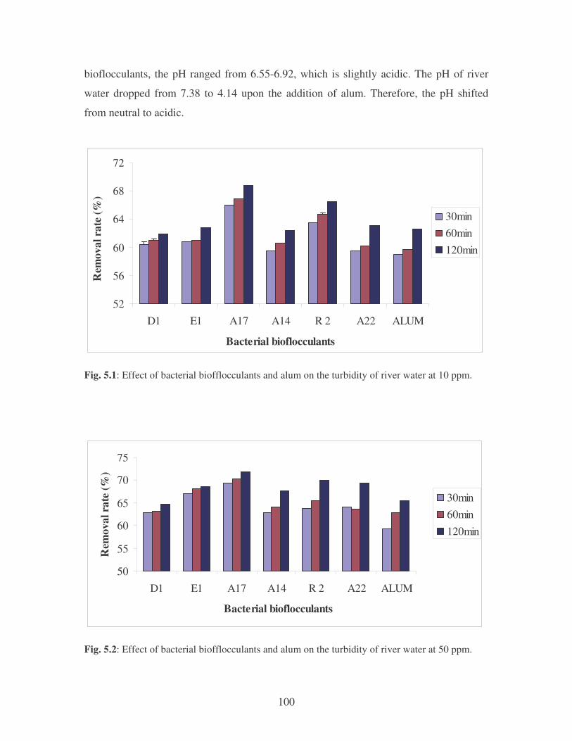
100
bioflocculants, the pH ranged from 6.55-6.92, which is slightly acidic. The pH of river
water dropped from 7.38 to 4.14 upon the addition of alum. Therefore, the pH shifted
from neutral to acidic.
52
56
60
64
68
72
D1 E1 A17 A14 R 2 A22 ALUM
Bacterial bioflocculants
Rem
oval
rat
e (%
)
30min60min120min
Fig. 5.1: Effect of bacterial biofflocculants and alum on the turbidity of river water at 10 ppm.
50
55
60
65
70
75
D1 E1 A17 A14 R 2 A22 ALUM
Bacterial bioflocculants
Rem
oval
rat
e (%
)
30min60min120min
Fig. 5.2: Effect of bacterial biofflocculants and alum on the turbidity of river water at 50 ppm.
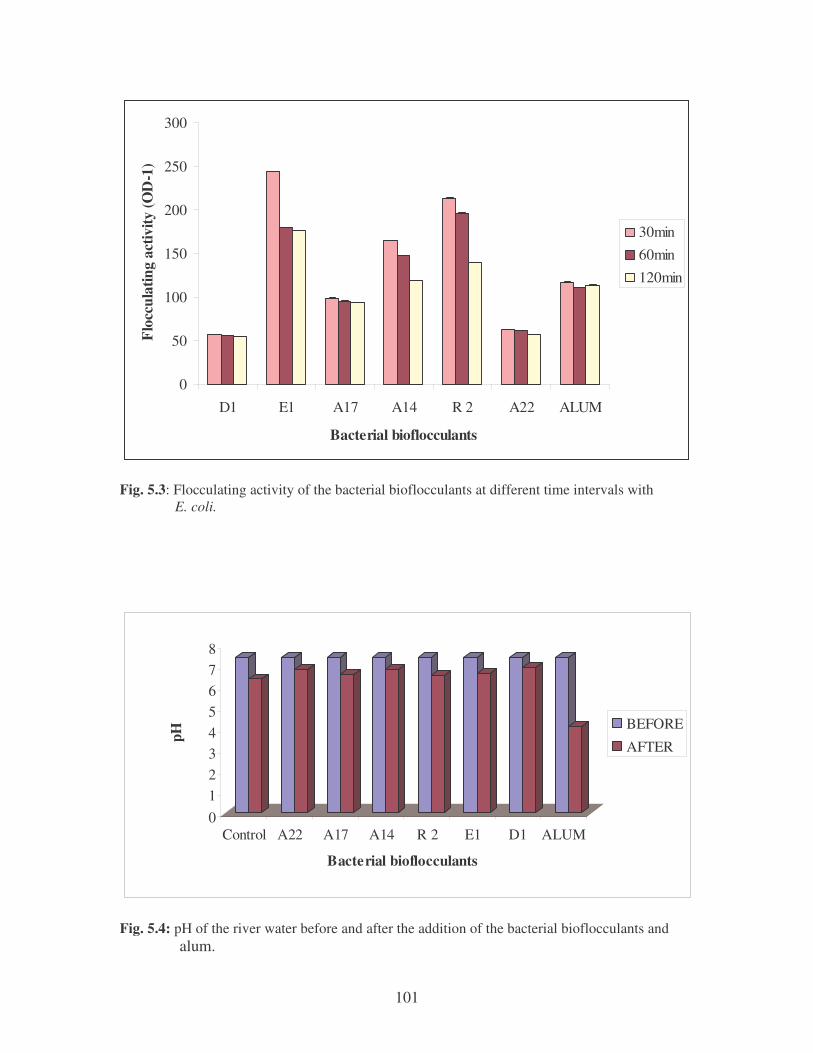
101
0
50
100
150
200
250
300
D1 E1 A17 A14 R 2 A22 ALUM
Bacterial bioflocculants
Floc
cula
ting
activ
ity (O
D-1
)
30min60min120min
Fig. 5.3: Flocculating activity of the bacterial bioflocculants at different time intervals with E. coli.
Fig. 5.4: pH of the river water before and after the addition of the bacterial bioflocculants and alum.
012345678
pH
Control A22 A17 A14 R 2 E1 D1 ALUM
Bacterial bioflocculants
BEFORE
AFTER
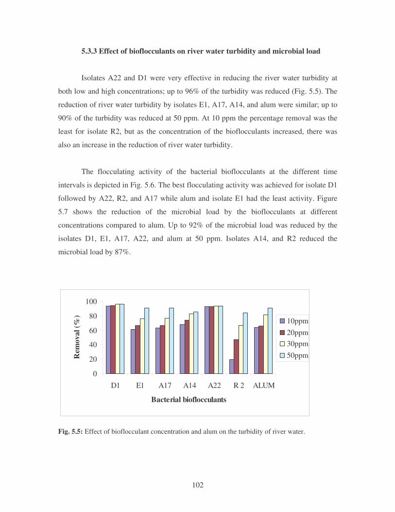
102
5.3.3 Effect of bioflocculants on river water turbidity and microbial load
Isolates A22 and D1 were very effective in reducing the river water turbidity at
both low and high concentrations; up to 96% of the turbidity was reduced (Fig. 5.5). The
reduction of river water turbidity by isolates E1, A17, A14, and alum were similar; up to
90% of the turbidity was reduced at 50 ppm. At 10 ppm the percentage removal was the
least for isolate R2, but as the concentration of the bioflocculants increased, there was
also an increase in the reduction of river water turbidity.
The flocculating activity of the bacterial bioflocculants at the different time
intervals is depicted in Fig. 5.6. The best flocculating activity was achieved for isolate D1
followed by A22, R2, and A17 while alum and isolate E1 had the least activity. Figure
5.7 shows the reduction of the microbial load by the bioflocculants at different
concentrations compared to alum. Up to 92% of the microbial load was reduced by the
isolates D1, E1, A17, A22, and alum at 50 ppm. Isolates A14, and R2 reduced the
microbial load by 87%.
0
20
40
60
80
100
D1 E1 A17 A14 A22 R 2 ALUM
Bacterial bioflocculants
Rem
oval
(%)
10ppm20ppm30ppm50ppm
Fig. 5.5: Effect of bioflocculant concentration and alum on the turbidity of river water.
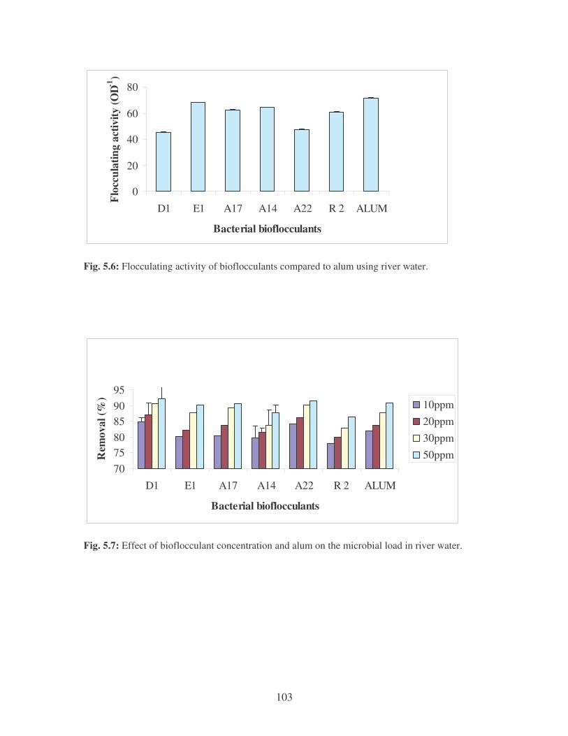
103
0
20
40
60
80
D1 E1 A17 A14 A22 R 2 ALUM
Bacterial bioflocculants
Floc
cula
ting
activ
ity (O
D-1)
Fig. 5.6: Flocculating activity of bioflocculants compared to alum using river water.
707580859095
D1 E1 A17 A14 A22 R 2 ALUM
Bacterial bioflocculants
Rem
oval
(%)
10ppm20ppm30ppm50ppm
Fig. 5.7: Effect of bioflocculant concentration and alum on the microbial load in river water.
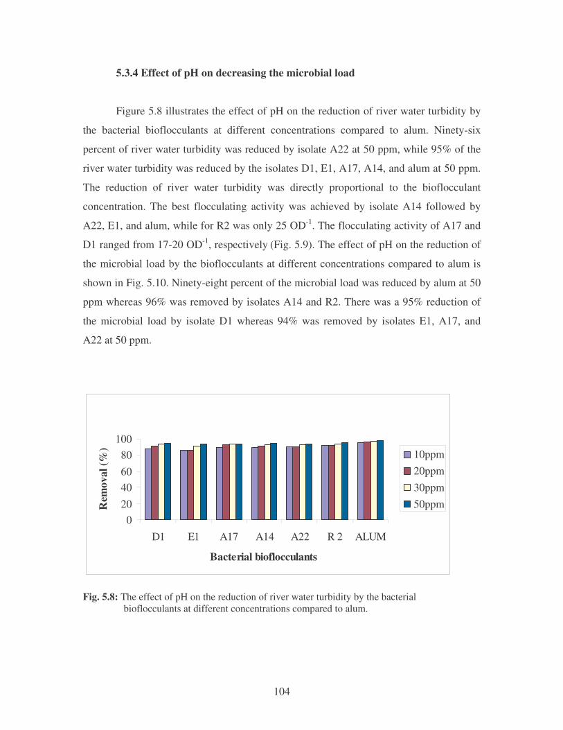
104
5.3.4 Effect of pH on decreasing the microbial load
Figure 5.8 illustrates the effect of pH on the reduction of river water turbidity by
the bacterial bioflocculants at different concentrations compared to alum. Ninety-six
percent of river water turbidity was reduced by isolate A22 at 50 ppm, while 95% of the
river water turbidity was reduced by the isolates D1, E1, A17, A14, and alum at 50 ppm.
The reduction of river water turbidity was directly proportional to the bioflocculant
concentration. The best flocculating activity was achieved by isolate A14 followed by
A22, E1, and alum, while for R2 was only 25 OD-1. The flocculating activity of A17 and
D1 ranged from 17-20 OD-1, respectively (Fig. 5.9). The effect of pH on the reduction of
the microbial load by the bioflocculants at different concentrations compared to alum is
shown in Fig. 5.10. Ninety-eight percent of the microbial load was reduced by alum at 50
ppm whereas 96% was removed by isolates A14 and R2. There was a 95% reduction of
the microbial load by isolate D1 whereas 94% was removed by isolates E1, A17, and
A22 at 50 ppm.
020406080
100
D1 E1 A17 A14 A22 R 2 ALUM
Bacterial bioflocculants
Rem
oval
(%) 10ppm
20ppm30ppm50ppm
Fig. 5.8: The effect of pH on the reduction of river water turbidity by the bacterial bioflocculants at different concentrations compared to alum.
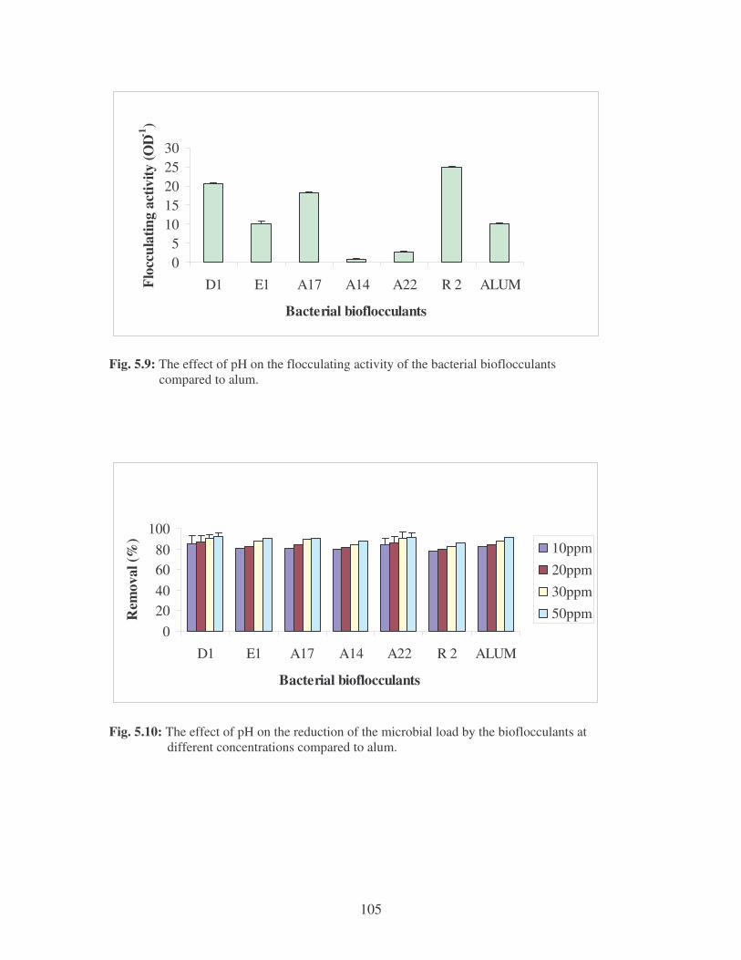
105
05
1015202530
D1 E1 A17 A14 A22 R 2 ALUM
Bacterial bioflocculants
Floc
cula
ting
activ
ity (O
D-1)
Fig. 5.9: The effect of pH on the flocculating activity of the bacterial bioflocculants compared to alum.
020406080
100
D1 E1 A17 A14 A22 R 2 ALUM
Bacterial bioflocculants
Rem
oval
(%)
10ppm20ppm30ppm50ppm
Fig. 5.10: The effect of pH on the reduction of the microbial load by the bioflocculants at different concentrations compared to alum.
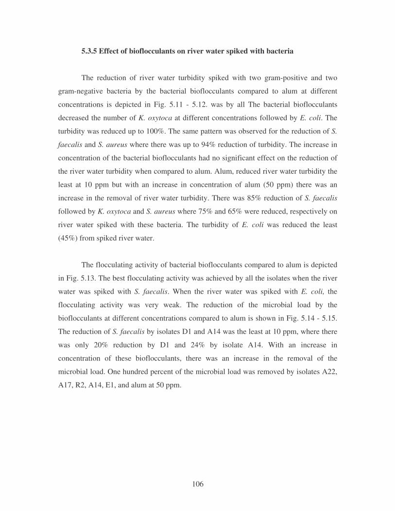
106
5.3.5 Effect of bioflocculants on river water spiked with bacteria
The reduction of river water turbidity spiked with two gram-positive and two
gram-negative bacteria by the bacterial bioflocculants compared to alum at different
concentrations is depicted in Fig. 5.11 - 5.12. was by all The bacterial bioflocculants
decreased the number of K. oxytoca at different concentrations followed by E. coli. The
turbidity was reduced up to 100%. The same pattern was observed for the reduction of S.
faecalis and S. aureus where there was up to 94% reduction of turbidity. The increase in
concentration of the bacterial bioflocculants had no significant effect on the reduction of
the river water turbidity when compared to alum. Alum, reduced river water turbidity the
least at 10 ppm but with an increase in concentration of alum (50 ppm) there was an
increase in the removal of river water turbidity. There was 85% reduction of S. faecalis
followed by K. oxytoca and S. aureus where 75% and 65% were reduced, respectively on
river water spiked with these bacteria. The turbidity of E. coli was reduced the least
(45%) from spiked river water.
The flocculating activity of bacterial bioflocculants compared to alum is depicted
in Fig. 5.13. The best flocculating activity was achieved by all the isolates when the river
water was spiked with S. faecalis. When the river water was spiked with E. coli, the
flocculating activity was very weak. The reduction of the microbial load by the
bioflocculants at different concentrations compared to alum is shown in Fig. 5.14 - 5.15.
The reduction of S. faecalis by isolates D1 and A14 was the least at 10 ppm, where there
was only 20% reduction by D1 and 24% by isolate A14. With an increase in
concentration of these bioflocculants, there was an increase in the removal of the
microbial load. One hundred percent of the microbial load was removed by isolates A22,
A17, R2, A14, E1, and alum at 50 ppm.
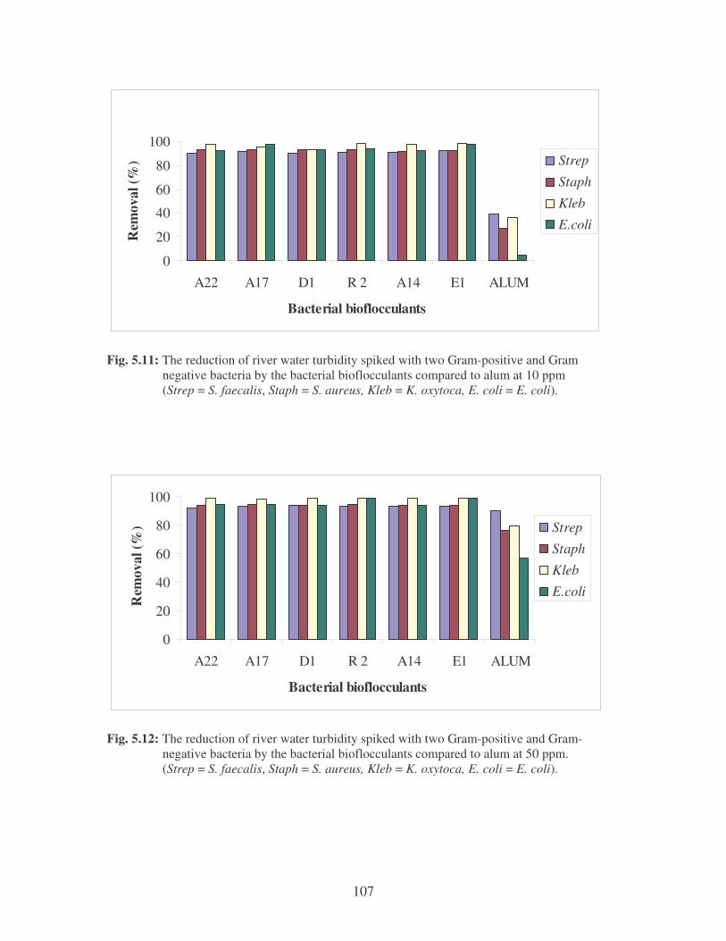
107
0
20
40
60
80
100
A22 A17 D1 R 2 A14 E1 ALUM
Bacterial bioflocculants
Rem
oval
(%) Strep
Staph
Kleb
E.coli
Fig. 5.11: The reduction of river water turbidity spiked with two Gram-positive and Gram negative bacteria by the bacterial bioflocculants compared to alum at 10 ppm (Strep = S. faecalis, Staph = S. aureus, Kleb = K. oxytoca, E. coli = E. coli).
0
20
40
60
80
100
A22 A17 D1 R 2 A14 E1 ALUM
Bacterial bioflocculants
Rem
oval
(%) Strep
Staph
Kleb
E.coli
Fig. 5.12: The reduction of river water turbidity spiked with two Gram-positive and Gram- negative bacteria by the bacterial bioflocculants compared to alum at 50 ppm. (Strep = S. faecalis, Staph = S. aureus, Kleb = K. oxytoca, E. coli = E. coli).
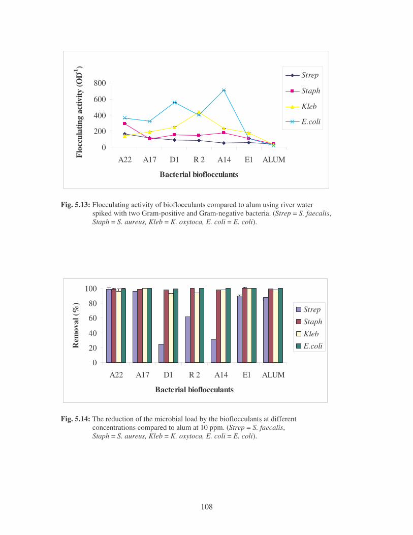
108
0
200
400
600
800
A22 A17 D1 R 2 A14 E1 ALUM
Bacterial bioflocculants
Floc
cula
ting
activ
ity (O
D-1)
Strep
Staph
Kleb
E.coli
Fig. 5.13: Flocculating activity of bioflocculants compared to alum using river water spiked with two Gram-positive and Gram-negative bacteria. (Strep = S. faecalis, Staph = S. aureus, Kleb = K. oxytoca, E. coli = E. coli).
0
20
40
60
80
100
A22 A17 D1 R 2 A14 E1 ALUM
Bacterial bioflocculants
Rem
oval
(%)
Strep
Staph
Kleb
E.coli
Fig. 5.14: The reduction of the microbial load by the bioflocculants at different concentrations compared to alum at 10 ppm. (Strep = S. faecalis, Staph = S. aureus, Kleb = K. oxytoca, E. coli = E. coli).

109
0
20
40
60
80
100
A22 A17 D1 R 2 A14 E1 ALUM
Bacterial bioflocculants
Rem
oval
(%)
Strep
Staph
Kleb
E.coli
Fig. 5.15: The reduction of the microbial load by the bioflocculants at different concentrations compared to alum at 50 ppm. (Strep = S. faecalis, Staph = S. aureus, Kleb = K. oxytoca, E. coli = E. coli).
5.4 DISCUSSION
River water turbidity decreased with an increase in flocculant concentration of 50
ppm, and then remained constant with a further increase in flocculant level. This occurs
because the optimum amount of flocculants in the suspension causes the microorganisms
and the fine particles to aggregate and settle. However, when the optimum concentration
of flocculant is exceeded it is known to cause the aggregated particles to redisperse and
this disturbs particle-settling (Chan and Chiang, 1995). Mishra et al. (2004) explained
that this behaviour could be based on an increase in the repulsive energy between the
flocculants and the microorganisms, which causes hindrance in floc formation.
The pH of the river water prior to the addition of the bacterial bioflocculants and
alum was neutral, with a subsequent decrease in pH upon the addition of bacterial
bioflocculants and alum. The addition of alum caused the pH to drop to 4.14, which is
more acidic, which means that in practical terms, further chemical addition is necessary
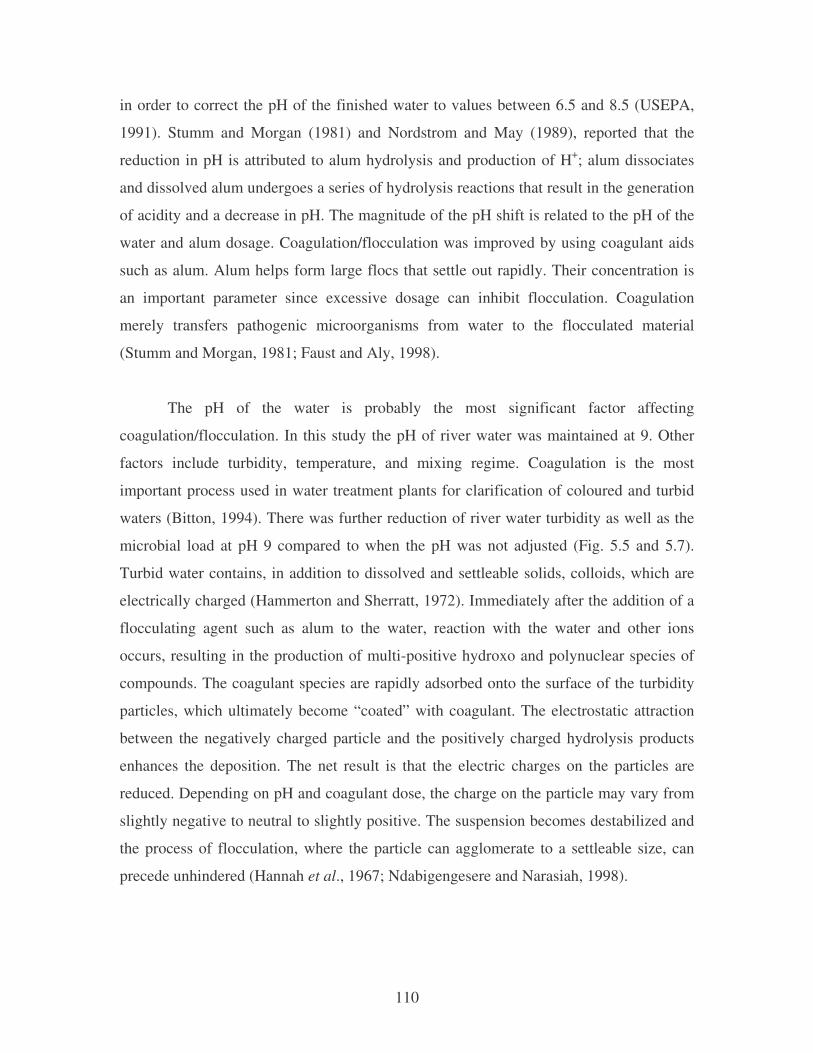
110
in order to correct the pH of the finished water to values between 6.5 and 8.5 (USEPA,
1991). Stumm and Morgan (1981) and Nordstrom and May (1989), reported that the
reduction in pH is attributed to alum hydrolysis and production of H+; alum dissociates
and dissolved alum undergoes a series of hydrolysis reactions that result in the generation
of acidity and a decrease in pH. The magnitude of the pH shift is related to the pH of the
water and alum dosage. Coagulation/flocculation was improved by using coagulant aids
such as alum. Alum helps form large flocs that settle out rapidly. Their concentration is
an important parameter since excessive dosage can inhibit flocculation. Coagulation
merely transfers pathogenic microorganisms from water to the flocculated material
(Stumm and Morgan, 1981; Faust and Aly, 1998).
The pH of the water is probably the most significant factor affecting
coagulation/flocculation. In this study the pH of river water was maintained at 9. Other
factors include turbidity, temperature, and mixing regime. Coagulation is the most
important process used in water treatment plants for clarification of coloured and turbid
waters (Bitton, 1994). There was further reduction of river water turbidity as well as the
microbial load at pH 9 compared to when the pH was not adjusted (Fig. 5.5 and 5.7).
Turbid water contains, in addition to dissolved and settleable solids, colloids, which are
electrically charged (Hammerton and Sherratt, 1972). Immediately after the addition of a
flocculating agent such as alum to the water, reaction with the water and other ions
occurs, resulting in the production of multi-positive hydroxo and polynuclear species of
compounds. The coagulant species are rapidly adsorbed onto the surface of the turbidity
particles, which ultimately become “coated” with coagulant. The electrostatic attraction
between the negatively charged particle and the positively charged hydrolysis products
enhances the deposition. The net result is that the electric charges on the particles are
reduced. Depending on pH and coagulant dose, the charge on the particle may vary from
slightly negative to neutral to slightly positive. The suspension becomes destabilized and
the process of flocculation, where the particle can agglomerate to a settleable size, can
precede unhindered (Hannah et al., 1967; Ndabigengesere and Narasiah, 1998).
111
Bacterial bioflocculants were very effective in reducing both the turbidity and the
microbial load of river water. Different bacterial isolates used to spike river water were
flocculated randomly by the bioflocculants (Fig. 5.11 − 5.15). In this study, there was a
maximum removal of microbial load and turbidity of river water by both the bacterial
bioflocculants and alum. Bitton (1994) indicated that removal of bacteria, although
variable may exceed 90% during the flocculation process, furthermore, coagulation
removes 74-99.4% of E. coli and coliforms. Kurane et al. (1986a) reported that the
flocculant produced by Rhodococcus erythropolis could efficiently flocculate all
suspended solids in aqueous solutions tested and had a wide flocculating activity against
both organic and inorganic materials. Among those effectively tested were
microrganisms such as E. coli, and alcohol yeast, activated sludge, Microcystis
aeruginosa (AOKO), kaolin clay, muddy water, river dredging water, river bottom
sediment (HEDORO), ash from a stream-power station and charcoal. Takagi and
Kadowaki (1985) reported that the Paecilomyces flocculant also had the ability to
flocculate all suspended solids from organic materials such as microorganisms to
inorganic materials such as aluminium oxide and that Paecilomyces flocculant was a
polysaccharide composed of galactosamine.
The application of bioflocculants for the reduction of microbial load and turbidity
from river water was examined in comparison with a conventional coagulant agent, alum
(Fig. 5.11 - 5.15). The results indicated that the bioflocculants were efficient for the
reduction of these bacteria as well as the turbidity. Furthermore, the bioflocculants
produced similar results as alum did, but at a slightly lower dosage. The use of alum
produced the best results in the removal of the microbial load (Fig. 5.15). Higher
concentrations of alum were required to reduce the river water turbidity compared to the
use of the bacterial bioflocculants (Fig. 5.11 and 5.13). This can be explained by the
production of aluminium hydroxide as a precipitate. In the case of bacterial
bioflocculants, only initial suspended particles are agglomerated into larger and settleable
flocs, but no additional precipitate is formed. Besides being voluminous, the alum
sludges are gelatinous, acidic, and difficult to dewater and dispose in the environment
(Degremont, 1989 − cited by Ndabigengesere and Narasiah, 1998). Faust and Aly (1998)
112
showed that alum was not effective in removing bacteria within the range of 5–10 mg/l.
A removal of 99.7% was achieved with 50 mg/l when 14 nephelometric units (NTU) of
turbidity was present.
Alum is a widely used coagulant in wastewater treatment. However, medical
reports indicated that aluminum might induce Alzheimer’s disease, while residual
aluminum concentrations in treated water can also impose health problems apart from the
production of high amounts of sludge (Letterman and Driscoll, 1988). The maximum
contaminant level of aluminum in drinking water was set to 200 µg/l (Zouboulisa et al.,
2004). Therefore, the use of high concentrations of alum in the treatment of river water
must be avoided.
High turbidity and/or colour impart an aesthetically displeasing appearance to
water. Apart from a displeasing appearance, turbidity provides adsorption sites for
biological organisms and interferes with disinfection. Only a turbidity of 1 NTU is
allowed in drinking water (Bitton, 1994). The river water used in this study is not suitable
for human consumption because the turbidity was 11.7 NTU. Compared with USEPA
Standards (1991), which state that the turbidity of drinking water should be less than 1
ntu, the value of 11.7 NTU is quite excessive. Although turbidity has no serious health
effects, it can interfere with disinfection and provide a medium for microbial growth.
Turbidity has been shown through scientific studies to be correlated with the
contamination of water supplies (typically surface water supplies) with Giardia and
Cryptosporidium (USEPA, 1991). Excessive turbidity is often associated with
unacceptable tastes, odours, and colour in water and may represent a health concern
where heavy metal ions, pesticides or waterborne disease causing organisms may attach
to the suspended particles. These organisms include bacteria, viruses, and parasites that
can cause symptoms such as nausea, cramps, diarrhoea, and associated headaches
(Vigneswaran and Visvanathan, 1995).
It is anticipated that bacterial bioflocculants will be utilized in the areas of
wastewater treatment. Due to their relative harmlessness towards humans and the
113
environment, they can also be used in drinking water, downstream processing, in food
and fermentation industry. Using natural coagulants in developing countries could
effectively alleviate their economic situation and allow further extension of water supply
in rural areas. The application of bacterial bioflocculants in the treatment of river water is
a promising alternative to using alum. To the best of our knowledge, this is the first study
demonstrating the use of bacterial bioflocculants for removal of microorganisms from
contaminated water and as such, it was difficult to compare the results with other
publications. The removal of organic and inorganic matter from river water using
bioflocculants is still in the research stages. However, more studies are required to
develop practical applications.
114
CHAPTER SIX
CONCLUDING REMARKS
6.1 THE RESEARCH IN PERSPECTIVE
The main objectives of this study were to characterize the properties of the
bioflocculants from bacteria, to evaluate the efficacy of the bioflocculant as an alternative
to alum in decreasing the microbial load of river water, and to evaluate the ability of the
bacterial bioflocculants to remove dyes and chemicals from the textile industries. Six
bioflocculant producing bacteria were isolated from Northern Wastewater Treatment
Plant. The bacterial isolates were identified and their bioflocculants were purified and
analyzed. The bioflocculants were found to be composed of carbohydrates, proteins,
uronic acid and amino sugars in varying quantities.
The bioflocculants produced by these bacteria were capable of flocculating kaolin
clay, dyes and microbes in river water. The results of the experiments described here
demonstrate that these flocculants could efficiently flocculate all suspended solids in
aqueous solution and had a wide flocculating activity against both inorganic and organic
materials. Flocculant concentration, temperature, pH, time, and cations or salts influenced
flocculation by increasing or decreasing the flocculating activity and percentage removal.
The bioflocculants produced by these bacterial strains had a satisfactory level of
flocculating activity. These results suggest that these bioflocculants can be successfully
applied for the clarification of river water or wastewaters under various environmental
conditions. These bioflocculants exhibited flocculating activity comparable or superior to
that of existing inorganic flocculants (alum), where up to 99% microbial load and
turbidity were reduced.
Coloured-dye-wastewater treatment and decolourization presents an arduous task.
Wide ranges of pH, salt concentrations, and chemical structures often add to the
115
complication (Banat et al., 1996; Pinheiro et al., 2004). This study revealed that the
bacterial isolates were capable of producing bioflocculants with very good flocculating
activity. The bioflocculants were effective to varying degrees in removing the dyes in
aqueous solution, in particular whale dye, medi-blue, fawn dye and mixed dyes, with a
decolourization efficiency ranging between 20-99.9%. Thus, these bioflocculants may be
used in the coagulation process instead of alum. However, more research still needs to be
conducted to optimize the conditions for maximum flocculation. Among the most
economically viable choices available for effluent treatment/decolourization, and the
most practical in terms of labour requirements and running expenses to adopt and
develop, appear to be the biological systems. At present, biological systems are known to
be capable of dealing with BOD and COD reduction or removal through conventional
aerobic biodegradation. They have however, an inherent problem in their inability to
remove colour (Banat et al., 1996).
Although decolourization is a challenging process to both the textile industry and
the wastewater-treatment facilities that must treat them, the literature suggests a great
potential for microbial decolourizing systems for achieving total colour removal and
(occasionally) with only a few hours of exposure. Such biological processes could be
adopted as a pre-treatment decolourization step, combined with the conventional
treatment system (e.g. activated sludge) to reduce the BOD and COD, as an effective
alternative for use by the textile-dyeing industries (Pereira et al., 2003). Concerted efforts
are still required to establish biological decolourization systems. The techniques by which
decolourization occurs vary and among them adsorption seems of great significance for
future development in bio-removal or bio-recovery of dye substances. It is important to
develop a novel biodegradable and eco-friendly organic coagulant without secondary
pollution for wastewater treatment. Unlike some synthetic flocculants, bioflocculants are
generally non-toxic and benign to the environment. They have a potential to improve
productivities and product quality in bioprocessing, wastewater treatment, and many
other industrial operations (Sanghi et al., 2006). Bioflocculants can be produced
relatively inexpensively from a variety of microorganisms. Microbial flocculation is a
116
promising alternative to replace or supplement present treatment processes for river water
and the removal of very high concentrations of dyes.
6.2 POTENTIAL FOR FUTURE DEVELOPMENT OF THIS WORK
Undoubtedly, low-cost bacterial bioflocculants offer many promising benefits for
commercial purposes in the future. However, despite a number of papers published on
low-cost flocculants, there is little information containing a full study of comparison
between flocculants. Although a lot has been accomplished in the area of flocculants,
more work is necessary (i) to predict the performance of the adsorption processes for dye
removal from industrial effluents under a range of operating conditions, (ii) to better
understand the flocculation or adsorption mechanisms and (iii) to demonstrate the use of
inexpensive flocculants at an industrial scale (Crini, 2006).
One of the routes still to be explored is the use of thermotolerant or thermophilic
microorganisms in decolourization systems. This would be of advantage as many textile
and other dye effluents are produced at relatively high temperatures (50-60°C), even after
a cooling or heat-exchange step. The availability of thermotolerant organisms may
consequently reduce cost significantly, through removing the need for further removal of
low-grade heat and through allowing more immediate treatment (Banat et al., 1996).
Techniques used in studies of polysaccharides, including chemical composition,
linkage pattern, and higher order structures are in constant development. They provide
information necessary for understanding of the polysaccharide properties and functions.
Recent advancements in studies of the polysaccharides at the single-molecule level are
essential. These techniques can be used to investigate properties of single molecules close
to physiological conditions. This field is expected to have increasing impact on the
further advancement of the molecular understanding of the role of polysaccharides in
various biological processes such as recognition and cell adhesion. Since the primary
structure of polysaccharides is not coded directly in the genetic sequence, the
advancement in primary structure determination has not evolved as rapidly within the
117
polysaccharide field as it has for proteins (Sletmoen et al., 2003). This, together with the
fact that the experimental procedures for determination of the relative contents and
arrangement of the monosaccharides are technically more demanding, makes the
description of the polysaccharide primary structure not an easy task.
The development of sensitive detection methods will provide very useful
information that will aid the structural elucidation of these extracellular polysaccharides.
The use of accurate equipment such as Fourier transform infrared, X-ray photoelectron
spectroscopy, and High performance liquid chromatography etc. in the future will aid in
the analysis of the chemical compositions of the extracellular polysaccharides. The role
of molecular biology has yet to feature prominently in this vital area of environmental
protection (Shubo et al., 2005). More research on these areas mentioned will offer a
better understanding of the function and properties of the bacterial bioflocculants.
118
REFERENCES
Aksu, Z. 2003. Reactive dye bioaccumulation by Saccharomyces cerevisiae. Process
Biochemistry. 38:1437-1444.
Aksu, Z. 2005. Application of biosorption for the removal of organic pollutants: a
review. Process Biochemistry. 40:997-1026.
Aksu, Z., and S. Tezer. 2000. Equilibrium and kinetic modelling of biosorption of
Remazol Black B by Rhizopus arrhizus in a batch system: effect of temperature. Process
Biochemistry. 36:431-439.
Atherton, F., C. P.C. Newman, and D. P. Casemore.1995. An outbreak of waterborne
cryptospondiosis associated with a public water supply in the UK. Epidemiology of
Infections. 115:123-131.
Banat, I M., P. Nigam, D. Singh, and R. Marchant. 1996. Microbial decolourization of
textile-dye-containing effluents. Bioresource Technology. 58:217-227.
Bar-Or, Y., and M. Shilo. 1987. Characterization of macromolecular flocculants
produced by Phormidium sp. J-1 and by Anabaenopsis circularis PCC 6720. Applied and
Environmental Microbiology. 53:2226-2230.
Baughman, G. L., and T. A. Perenich. 1988. Fate of dyes in aquatic systems: I.
Solubility and partitioning of some hydrophobic dyes and related compounds.
Environmental Toxicological Chemistry. 7:183-199.
Bender, J., E. R. Archibold, V. Ibeanusi, and J. P. Gould. 1989. Lead removal from
contaminated water by a mixed microbial ecosystem. Water Science Technology.
21:1661-1665.
119
Bhattacharyya, K. G., and A. Sarma. 2003. Adsorption characteristics of the dye,
brilliant green, on neem leaf powder. Dyes Pigments. 57:211-222.
Bitton, G. 1994. Wastewater microbiology, p. 265-266. In R. Mitchell (ed.), Division of
applied sciences. Harvard University. John Wiley and Sons Ltd., New York.
Black, A. P., F. B. Birkner, and J. J. Morgan. 1966. The effect of polymer adsorption
on the electrokinetic stability of dilute clay suspension. Journal of Colloidal and
Interface Science. 21:626.
Bragger, J. L., A. W. Lloyd, S. H. Soozandehfar, S. F. Bloomfield, C. Marriott, and
G. P. Martin. 1997. Investigations into the azo reducing activity of a common colonic
microorganism. International Journal of Pharmaceutics. 157:61-71.
Bras, R., I. A. Ferra, H. M. Pinheiro, and I. C. Goncalves. 2001. Batch tests for
assessing decolourisation of azo dyes by methanogenic and mixed cultures. Journal of
Biotechnology. 89:155-162.
Brugha, A., I. B. Vipond, and M. R. Evans. 1999. A community outbreak of food
borne small round-structured virus gastroenteritis caused by a contaminated water supply.
Epidemiology of Infections. 122:145-154.
Brosius, J., J. L. Palmer, H. P. Kennedy, and H. F. Nuller. 1978. Complete nucleotide
sequence of a 16S ribosomal RNA gene from Escherichia coli. Proceedings of the
National Academy of Sciences. 75: 4801-4805.
Buchhammer, H. M., M. Oelmann, and G. Petzold. 2001. Flocculation of disperse
dyes in effluents with polyelectrolyte complexes. Melliand English. 82: 104-105.
120
Butterfield, C. T. 1935. A Zoogloea-forming bacterium isolated from activated sludge,
studies of sewage purification (II). Public Health Report. 50:671-681.
Chan, W. C., and C. Y. Chiang. 1995. Flocculation of clay suspensions with water-
insoluble starch grafting acrylamide/sodium allylsulfonated copolymer powder. Applied
Polymer Science. 58:1721-1726.
Chandrasekhar, S., and S. Ramaswamy. 2006. Iron minerals and their influence on the
optical properties of two Indian kaolins. Applied Clay Science. 33:269-277.
Chang, J. S., C. Chou, Y. C. Lin, P. J. Lin, J. Y. Ho, and T. L. Hu. 2001. Kinetic
characteristics of bacterial azo-dye decolourization by Pseudomonas luteola. Water
Research. 35:2841-2850.
Chang, J. S., and Y. C. Lin. 2000. Fed-batch bioreactor strategies for microbial
decolourization of azo dye using a Pseudomonas luteola strain. Biotechnology Progress.
16:979–85.
Chaplin, M. F. 1994. Monosaccharides, p. 2-6. In M. F. Chaplin & J. F. Kennedy (ed.),
Carbohydrate analysis: a practical approach, Oxford University Press, New York.
Cheng, X., and L. A. Kaplan. 2003. Simultaneous analyses of neutral carbohydrates and
amino sugars in freshwaters with HPLC-PAD. Journal of Chromatographic Science.
41:1-5.
Choy, J. H., W. S. Shin, S. H. Lee, D. J. Joo, and J. D. Lee. 2001. Application of
synthetic polyamine flocculants for dye wastewater treatment. Science and Technology.
36(13):2945–2958.
Chu, H.C., and K. M. Chen. 2002. Reuse of activated sludge biomass: removal of basic
dyes from wastewater by biomass. Process Biochemistry. 37:595-600.
121
Clarke, E. A., and R. Anliker. 1980. Organic dyes and pigments, p. 181-215. In O.
Hutzinger (ed.), Handbook of environmental chemistry, anthropogenic compounds, vol.
3, part A. Springer-Verlag, New York.
Cohen, J. M., G. A. Rourke, and R. L. Woodward. 1972. Natural and synthetic
polyelectrolyte as coagulant aids. Journal of Agriculture of Western Australia. 50:463-
471.
Cowan, R. M., N. G. Love, S. M. Sock, and K. White. 1995. Activated sludge and
other aerobic suspended culture processes. Water Environment Resource. 67:433-450.
Cowan, M. K., and K. P. Talaro. 2006. Microbiology: A systems approach 1st ed., p.
785-786. The McGraw-Hill, Inc., New York.
Crini, G. 2006. Non-conventional low-cost adsorbents for dye removal. Bioresource
Technology. 97:1061-1085.
Crittenden, J. C., R. P. S. Suri, D. L. Perram, and D. W. Hand. 1997.
Decontamination of water using adsorption and photocatalysis. Water Resource. 31:411-
418.
Dabrowski, A. 2001. Adsorption, from theory to practice. Advances in Colloid Interface
Science. 93:135-224.
Deng, S. B., R. B. Bai, X. M. Hu, and Q. Luo. 2003. Characteristics of a bioflocculant
produced by Bacillus mucilaginosus and its use in starch and wastewater treatment.
Applied Microbiology and Biotechnology. 60:588-593.
Decker, K. C., and B. W. Long. 1992. Canada’s cooperative approach to drinking water
regulations. Journal of Wastewater Analysis. 84:120-127.
122
Dermlim, W., P. Prasertsan, and H. Doelle. 1999. Screening and characterization of
bioflocculant produced by isolated Klebsiella sp. Applied Microbiology and
Biotechnology. 52:698-703.
De Vuyst, L., F. De Vin, F. Vaningelgem, and B. Degeest. 2001. Recent developments
in the biosynthesis and applications of heteropolysaccharides from lactic acid bacteria.
International Dairy Journal 11: 687-707.
Dhodapkar, R., N. N. Rao, S. P. Pande, and S. N. Kaul. 2006. Removal of basic dyes
from aqueous medium a novel polymer: Jalshakti. Bioresource Technology. 97:877-885
Dillert, R., S. Vollmer, M. Schober, J. Theurieh, D. Bahnemann, H. J. Amtz, K.
Pahlmann, and J. Wienefeld. 1999. Photocatalytic treatment of an industrial wastewater
in the double-skin sheet reactor. Chemical Engineering and Technology. 22:931-934.
DiTerlizzi, S., and B. Fall. 1994. Coagulation and flocculation of wastewater, p. 414-
415. John Wiley and Sons Ltd., New York.
Dönmez, G. 2002. Bioaccumulation of the reactive textile dyes by Candida tropicalis
growing in molasses medium. Enzyme and Microbial Technology. 30:363-366.
Dos Santos, A. B., F. J. Cervantes, and J. B. van Lier. 2007. Current technologies for
decolourization of textile wastewaters: perspectives for anaerobic biotechnology.
Bioresource Technology. doi:10.1016/j.biortech.2006.11.013.
Dos Santos, A. B., M. P. Madrid, F. A. M. de Bok, A. J. M. Stams, J. B. Van Lier,
and F. J. Cervantes. 2006. The contribution of fermentative bacteria and methanogenic
archaea to azo dye reduction by thermophilic anaerobic consortium. Enzyme and
Microbial Technology. 39:38-46.
Dube, J. 1992. Microorganisms as chemical reagents. Minerals Engineering. 5:547-556.
123
Dudman, W. F. 1977. The role of surface polysaccharides in natural environments, p.
357-414. In I. Sutherland (ed.), Surface carbohydrates of the prokaryotic cell. Academic
Press Inc., New York.
Egorov, A. I., A. A. Tereschenko, L. M. Altshul, T. Vartiainen, D. Samsonov, B.
LaBrecque, J. Mäki-Paakkanen, N. L. Drizhd, and T. E. Ford. 2003. Exposures to
drinking water chlorinated by-product in a Russian city. International Journal of Hygiene
and Environmental Health. 206:539-551.
El-Geundi, M. S. 1991. Colour removal from textile effluents by adsorption techniques.
Water Resource. 25:271-273.
Elwood, D. C., and D. W. Tempest. 1972. Effect of environment on bacterial wall
content and composition. Advances in Microbial Physiology. 7:83-117.
Eriksson, L., and B. Alm. 1991. Study of flocculation mechanisms by observing effects
of a complexing agent on activated sludge properties. Water Science and Technology.
24:21-25.
Faust, S. D., and O. M. Aly. 1998. Chemistry of water treatment 2nd ed., p. 581 CRC
Press LLC, Lewis Publishers, New York.
Fazio, S. A., D. J. Uhlinger, J. H. Parker, and D. C. White. 1982. Estimations of
uronic acids as quantitative measures of extracellular and cell wall polysaccharide
polymers from environmental samples. Applied and Environmental Microbiology.
43:1151-1159.
Fewson, C. A. 1988. Biodegradation of xenobiotic and other persistent compounds: the
causes of recalcitrance. Trends in Biotechnology. 6:148-153.
124
Ford, T. E. 1993. Aquatic microbiology: an ecological approach, p. 9-13. In T. E. Ford
(ed.), Combridge, Mass Blackwell Scientific publications, Inc., New York.
Foster, C. F. 1983. Bound water in sewage sludges and its relationship to sludge surfaces
and sludge viscosities. Journal of Chemical Technology and Biotechnology. 33:76-80.
Fu, Y., and T. Viraraghavan. 2001. Fungal decolourization of wastewaters.
Bioresource Technology. 79:251-262.
Fu, Y., and T. Viraraghavan. 2002. Removal of Congo red from an aqueous solution by
fungus Aspergillus niger. Advances in Environmental Resource. 7:239-247.
Fumio, Y. 1991. Flocculation of yeast cells by Lactobacillus fermentum. Resource
Microbiology. 22:12-16.
Fujita, M., M. Ike, S. Tachibana, G. Kitada, S. M. Kim, and Z. Inoue. 2000.
Characterization of a bioflocculant produced by Citrobacter sp. TKF04 from acetic and
propionic acids. Journal of Bioscience and Bioengineering. 89:40-46.
Garrity, G M. 2005. Bergey's Manual of Systematic Bacteriology (Vol. 2, Part A,B,C),
p. 35-127. Springer, New York.
Ghoreishi, S. M., and R. Haghighi. 2003. Chemical catalytic reaction and biological
oxidation for treatment of non-biodegradable textile effluent. Journal of Chemical
Engineering. 95:163-169.
Gingell, R., and R. Walker. 1971. Mechanisms of azo reduction by Streptococcus
faecalis: the role of soluble flavins. Xenobiotica. 1:231-239.
125
Glenn, J. K., and M. H. Gold. 1983. Decolourization of several polymeric dyes by the
lignin degrading basidiomycete, Phanerochaete chrysosporium. Applied and
Environmental Microbiology. 45:1741-1747.
Guirand, J. 1992. Isolation and characterization of a flocculating mutant of
Saccharomyces diastaticus. Resource Microbiology. 1433:81-91.
Gupta, G. S., G. Prasad, and V. H. Singh. 1990. Removal of chrome dye from aqueous
solutions by mixed adsorbents: fly ash and coal. Water Resource. 24:45-50.
Hammerton, C., and J. G. Sherratt. 1972. Analysis of raw, potable and wastewater, p.
304. Great Britain, Department of the Environment, London. H.M.S.O.
Hannah, S. A., J. M. Cohen, and G. C. Robeck. 1967. Control techniques for
coagulation-filtration. Journal of Agriculture of Western Australia. 59:1149-1152.
Hantula, J., and D. H. Bamford. 1991a. The efficiency of the protein dependent
flocculation of Flavobacterium sp. Applied Microbiology and Biotechnology. 36:100-
104.
Hantula, J., and D. H. Bamford. 1991b. Bacterial phage resistance and flocculation
deficiency of Flavobacterium sp. are phenotypically interrelated. Applied Microbiology
and Biotechnology. 36:105-108.
Higgins, M. J. 1995. The roles and interactions of metal salts, proteins, and
polysaccharides in the settling and dewatering of activated sludge. Ph.D. thesis. Virginia
Polytechnic Institute and State University, Blacksburg, Virginia.
Hitz, H. R., W. Huber, and R. H. Reed. 1978. The absorption of dyes on activated
sludge. Journal of the Society of Dyers and Colourists. 94:71-76.
126
Ho, Y. S., and G. McKay. 1999. Comparative sorption kinetic studies of dye and
aromatic compounds onto fly ash. Journal of Environmental Science Health. 34:1179-
1204.
http://web.deu.edu.tr/atiksu/toprak/summary4.html
http://www.usgcrp.gov/usgcrp/images/ocp2003/WaterCycle-optimized.jpg
Huang, L. 1990. Studies on culture condition for production of flocculant by bacterial
strain S-4K. International Journal of Mineral Processing. 129:11-19.
Huang, C., and H. Shui. 1996. Interaction between alum and organics in coagulation,
p.113-163. John Wiley and Sons Ltd., New York.
Hu, T. L. 1992. Sorption of reactive dyes by Aeromonas biomass. Water Science
Technology. 26:357-366.
Hu, Y., and X. Liu. 2003. Chemical composition and surface property of kaolins.
Minerals Engineering. 16:1279-1284.
Hunter, P. R., and C. Quigley. 1998. Investigation of an outbreak of cryptospondiosis
associated with treated surface water finds limits to the value of case control studies.
Communicable disease and public health. 1(4):234-238.
Jansson, P. E., J. Lindberg, K. M. Wimalsiri, and M. A. Dankert. 1993. Structural
studies of acetan, an exopolysaccharide elaborated by Acetobacter xylinum.
Carbohydrate Resource. 245:303-310.
Jin, Y., and A. Speers. 1998. Flocculation of Saccharomyces cerevisiae. Food Research
International. 31:421-440.
127
Jones, M. N. 1998. Colloidal properties of humic substances. Advances in Colloid
Interface Science. 78:1-48.
Johnson, S. B., G. V. Franks, P. J. Scales, D. V. Boger, and T. W. Healy. 2000.
Surface chemistry–rheology relationships in concentrated mineral suspensions.
International Journal of Mineral Processing. 58:267-304.
Juang, R. S., R. L. Tseng, F. C. Wu, and S. H. Lee. 1997. Adsorption behaviour of
reactive dyes from aqueous solutions on chitosan. Journal of Chemistry, Technology and
Biotechnology. 70:391-399.
Kakii, K., M. Hasumi, T. Shirakashi, and M. Kuriyama. 1990. Involvement of Ca2+ in
the flocculation of Kluyvera cryocrescens KA-103. Journal of Fermentation and
Bioengineering. 69:224-227.
Kapdan, K., I. Kargi, G. McMullan, and R. Marchant. 2000. Effect of environmental
conditions on biological decolourization of textile dyestuff by Coriolus versicolor.
Enzyme and Microbial Technology. 26:381-387.
Karcher, S., A. Kornmuller, and M. Jekel. 1999. Removal of reactive dyes by
sorption/complexation with cucurbituril. Water Science Technology. 40:425-433.
Keck, A., J. Klein, M. Kudlich, A. Stolz, H. J. Knackmuss, and R. Mattes. 1997.
Reduction of azo dyes by redox mediators originating in the naphthalenesulfonic acid
degradation pathway of Sphingomonas sp. strain BN6. Applied and Environmental
Microbiology. 63:3684-3690.
Khan, A. A., and Q. Husain. 2007. Decolorization and removal of textile and non-
textile dyes from polluted wastewater and dyeing effluent by using potato (Solanum
tuberosum) soluble and immobilized polyphenol oxidase. Bioresource Technology.
98:1012-1019.
128
Kim, Y. 1993. The production and properties of exo-polysaccharides (POL-IIs) by
Bacillus sp. LK-1. Korean Journal of Applied Microbiology and Bioengineering. 21:478-
485.
Kiss, J. 1974. Beta-elimination degradations of carbohydrates containing uronic acid
residues. Advances in Carbohydrates, Chemistry and Biochemistry. 29:229-303.
Knackmuss, H. J. 1996. Basic knowledge and perspectives of bioelimination of
xenobiotic compounds. Journal of Biotechnology. 51:287-295.
Knapp, J. S., and P. S. Newby. 1999. The decolourization of a chemical industry
effluent by white rot fungi. Water Resource. 33:575-577.
Konan, K. L., C. Peyratout, J. Bonnet, A. Smith, A. Jacquet, P. Magnoux, and P.
Ayrault. 2006. Surface properties of kaolin and illite suspensions in concentrated
calcium hydroxide medium. Journal of Colloid and Interface Science.
doi:10.1016/j.jcis.2006.10.085
Kudlich, M., A. Keck, J. Klein, and A. Stolz. 1997. Localization of the enzyme system
involved in anaerobic reduction of azo dyes by Sphingomonas sp. strain BN6 and effect
of artificial redox mediators on the rate of azo dye reduction. Applied and Environmental
Microbiology. 63:3691-3694.
Kuhn, I., G. Allestam, M. Engdahl, and A. A. Stenstrom. 1997. Biochemical
fingerprinting of coliform bacterial populations comparisons between polluted river water
and factory effluents. Water Science and Technology. 35:343-350.
Kurane, R., K. Hatamochi, T. Kakuno, M. Kiyohara, K. Kawaguchi, Y. Mizuno, M.
Hirano, and Y. Taniguchi. 1994a. Production of a bioflocculant by Rhodococcus
erythropolis S-l grown on alcohols. Bioscience, Biotechnology and Biochemistry. 58:428-
429.
129
Kurane, R., K. Hatamochi, T. Kakuno, M. Kiyohara, K. Kawaguchi, Y. Mizuno, M.
Hirano, and Y. Taniguchi. 1994b. Purification and characterization of lipid
bioflocculant produced Rhodococcus erythropolis. Bioscience, Biotechnology and
Biochemistry. 58:1977-1982.
Kurane, R., K. Hatamochi, T. Kakuno, M. Kiyohara, T. Tajima, M. Hirano, and Y.
Taniguchi. 1995. Chemical structure of lipid bioflocculant produced by Rhodococcus
erythropolis. Journal of Agricultural and Biological Chemistry. 59:1652-1656.
Kurane, R., S. Hatakeyama, and H. Tsugeno. 1991 Correlation between flocculation
production and morphological changes in Rhodococcus erythropolis S-1. Journal of
Fermention and Bioengineering. 72:498-500.
Kurane, R., and H. Matsuyama. 1994. Production of bioflocculant by mixed culture.
Bioscience, Biotechnology and Biochemistry. 58:1589-1594.
Kurane, R., and Y. Nohata. 1991. Microbial flocculation of waste liquids and oil
emulsion by a bioflocculant from Alcaligenes latus. Journal of Agricultural and
Biological Chemistry. 56:1127-1129.
Kurane, R., K. Toeda, K. Takeda, and T. Suzuki. 1986a. Screening for and
characteristics of microbial flocculants. Journal of Agricultural and Biological
Chemistry. 50(9):2301-2307.
Kurane, R., K. Toeda, K. Takeda, and T. Suzuki. 1986b. Culture conditions for
production of microbial flocculant by Rhodococcus erythropolis. Journal of Agricultural
and Biological Chemistry. 50:2309-2313.
La-Mer, V. K., and T. W. Healy. 1963. Adsorption-flocculation reactions of
macromolecules at the solid-liquid interface. Reviews in Pure and Applied Chemistry
13:112.
130
Lambert, S. D., N. J. D. Graham, C. J. Sollars, and G. D. Fowler. 1997. Evaluation of
inorganic adsorbents for the removal of problematic textile dyes and pesticides. Water
Science Technology. 36:173-180.
Lee, S. H., S. O. Lee, K. L. Jang, and T. H. Lee. 1995. Microbial flocculant from
Arcuadendron sp. TS-49. Biotechnology Letters. 17:95-199.
Lee, C. K., K. S. Low, and P. Y. Gan. 1999. Removal of some organic dyes by acid-
treated spent bleaching earth. Process Biochemistry. 34:45-465.
Lerch, A., S. Panglisch, P. Buchta, Y. Tomita, H. Yonekawa, K. Hattori, and R.
Gimbel. 2005. Direct river water treatment using coagulation/ceramic membrane
microfiltration. Desalination. 179:41-50.
Letterman, R. D, and C. T. Driscoll. 1988. Survey of residual aluminum in filtered
water. Journal of Water Works Association. 80:154-158.
Lian, B., Y. Chen, J. Zhao, H. H. Teng, L. Zhu, and S. Yuan. 2007. Microbial
flocculation by Bacillus mucilaginosus: applications and mechanisms. Bioresource
technology. doi:10.1016/j.biortech.2007.09.045.
Li, J., M. Li, J. Li, and H. Sun. 2007. Decolourization of azo dye direct scarlet 4BS
solution using exfoliated graphite under ultrasonic irradiation. Ultrasonics
Sonochemistry. 14:241-245.
Lopez, E., I. Ramos, and M. A. Sanroman. 2003. Extracellular polysaccharides
production by Arthrobacter viscosus. Journal of Food Engineering. 60:463-467.
Lourenco, N. D, J. M. Novais, and H. M. Pinheiro. 2000. Reactive textile dye colour
removal in a sequencing batch reactor. Water Science and Technology. 42:321-328.
131
Low, K. S., and C. K. Lee. 1997. Quaternized rice husk as sorbent for reactive dyes.
Bioresource Technology. 61:121-125.
Manu, B., and S. Chaudhari. 2001. Anaerobic decolourization of simulated textile
wastewater containing azo dyes. Bioresource Technology. 82:225-231.
Manero, A., and A. R. Blanch. 1999. Identification of Enterococcus sp. with a
biochemical key. Applied and Environmental Microbiology. 65:4425-4430.
Marchesi, J. R., T. Sato, A. J. Weightman, T. A. Martin, J. C. Fry, S. J. Hiom, D.
Dymock, and W. G. Wade. 1998. Design and evaluation of useful bacterium-specific
PCR primers that amplify genes coding for 16S rRNA. Applied and Environmental
Microbiology. 64: 795-799.
Marco, A., S. Esplugas, and G. Saum. 1997. How and why to combine chemical and
biological processes for wastewater treatment. Water Science Technology. 35:231-327.
McCurdy, M. W., G. D. Boardman, D. L. Michelsen, and B. M. Woodby. 1992.
Chemical reduction and oxidation combined with biodegradation for the treatment of a
textile dye, p. 229-234. In 46th Proc. Purdue Industrial Waste Conf. Lewis Publishers,
Florida.
McKinney, R. E. 1956. Biological flocculation. Biological treatment of sewage and
industrial wastes. 1:88-117.
McKinney, R. E. 1957. Activity of microorganisms in organic waste disposal aerobic
processes. Applied Microbiology. 5:167-174.
McMullan, G., C. Meehan, A. Conneely, N. Kirby, T. Robinson, P. Nigam, I. M.
Banat, R. Marchant, and W. F. Smyth. 2001. Microbial decolourization and
degradation of textile dyes. Applied Microbiology Biotechnology. 56:81-87.

132
Meehan, C., I. M. Banat, G. McMullan, P. Nigam, F. Smyth, and R. Marchant.
2000. Decolourization of remazol-black using a thermotolerant yeast, Kluyveromyces
marxianus IMB3. Environmental Biotechnology. 26:75-79.
Meng, Y, X. Huang, Q. Yang, Y. Qian, N. Kubota, and S. Fukunaga. 2005. Treatment
of polluted river water with a photocatalytic slurry reactor using low-pressure mercury
lamps coupled with a membrane. Desalination. 181:121-133.
Meyer, U. 1981. Biodegradation of synthetic organic colorants, p. 371-385. In T.
Leisinger, A. M. Cook, R. Hutter and J. Nuesch. (ed.), Microbial degradation of
xenobiotic and recalcitrant compounds, FEMS Symposium 12th ed. Academic Press,
London.
Mezrioui, N., and B. Baleux. 1994. Resistance patterns of E. coli strains isolated from
domestic sewage before and after treatment in both aerobic lagoon and activated sludge.
Water Research. 28:2394-2406.
Mishra, G., and M. Tripathy. 1993. A critical review of the treatment for
decolourization of textile effluent. Colourage. 40:35-38.
Mishra, A., M. Yadav, B. Agarwal, and S. Rajani. 2004. Use of polyacrylamide-
grafted Plantago psyllium mucilage as a flocculant for treatment of textile wastewater.
Colloid Polymer Science. 282:722-727.
Mishra, A., and M. Bajpai. 2005. Flocculation behaviour of model textile wastewater
treated with a food grade polysaccharide. Journal of Hazardous Material. B118:213-217.
Misra, M. 2002. Selective flocculation of fine coal with hydrophobic Mycobacterium
phlei. Minerals and Metallurgical Processing. 10:20-23.

133
Mittal, A. K., and S. K. Gupta. 1996. Biosorption of cationic dyes by dead macro-
fungus Fomitopsis carnea: batch studies. Water Science Technology. 34:157-181.
Morais, L. C., O. M. Freitas, E. P. Gonçalves, L. T. Vasconcelos, and C. G. Gonzalez
Beça. 1999. Reactive dyes removal from wastewaters by adsorption on eucalyptus bark:
variables that define the process. Water Resource. 33:979-988.
Moran, C., M. E. Hall, and R. C. Howell. 1997. Effects of sewage treatment on textile
effluent. Journal of Social Dyers Colour. 113:272-274.
Morgan, J., C. Foster, and L. Evison. 1990. A comparative study of the nature of
biopolymers extracted from activated sludges. Water Resource. 24:743-750.
Muller, J. P., A. Manceau, G. Calas, T. Allard, P. Ildefone, and J. L. Hazemann.
1995. Crystal chemistry of kaolinite and Fe–Mn oxides: relation with formation condition
of low-temperature systems. American Journal of Science. 295:1115–1155.
Myers, C. R., and J. M. Myers. 1992. Localization of cytochromes to the outer
membrane of anaerobically grown Shewanella putrefaciens MR-1. Journal of
Bacteriology. 174:3429-3438.
Nakamura, J., S. Miyashiro, and Y. Hirose. 1976a. Screening, isolation, and some
properties of microbial cell flocculants. Agricultural and Biological Chemistry. 40:377-
383.
Nakamura, J., S. Miyashiro, and Y. Hirose. 1976b. Purification and chemical analysis
of microbial cell flocculant produced by Aspergillus sojae AJ7002. Agricultural and
Biological Chemistry. 40:619-624.
134
Nakamura, J., S. Miyashiro, and Y. Hirose. 1976c. Conditions of production of
microbial cell flocculant by Aspergillus sojae AJ-7002. Agricultural and Biological
Chemistry. 40:1341-1347.
Nakata, K., and R. Kurane. 1999. Production of extracellular polysaccharide
biofloccculants by Klebsiella pneumoniae. Journal of Bioscience, Biotechnology and
Biochemistry. 63:2064-068.
Napoli, C., F. Dazzo, and D. Hubbell. 1975. Production of cellulose microfibrils by
Rhizobium. Applied Microbiology. 30:123-131.
Navin, K., C. Twarakavi, and J. Kaluarachchi. 2006. Sustainability of ground water
quality considering land use changes and public health risks. Journal of Environmental
Management. 81:405-419.
Ndabigengesere, A., and K. S. Narasiah. 1998. Quality of water treated by coagulation
using Moringa oleifera seeds. Water Resources. 32(3):781-791.
Nester, E. W., D. G. Anderson, C. E. Roberts, N. N. Pearcal, and M. T. Nester. 2001.
Microbiology: a human perspective third edition, p. 787-799. The McGraw-Hill, Inc.,
New York.
Nguyen, A. L., S. Grothe, and J. H. T. Loung. 1988. Lactose hydrolysis in aqueous two
-phase system by whole-cell ß- galactosidase of Kluyveromyces marxianus. Applied
Microbiology and Biotechnology. 27:341-346.
Nigam, P., I. M. Banat, D. Singh, and R. Marchant. 1996. Microbial process for the
decolourization of textile effluent containing azo, diazo, and reactive dyes. Process
Biochemistry. 31(5):435-42.

135
Norberg, A. B., and S. O. Enfors. 1982. Production of extracellular polysaccharide by
Zoogloea ramigera. Applied and Environmental Microbiology. 44:1231-1237.
Nordstrom, D. K., and H. M. May. 1989. Aqueous equilibrium data for mononuclear
aluminum species, p. 29-55. In G. Spositio, (ed.), The environmental chemistry of
aluminum, CRC Press, Boca Raton. Florida.
Ogawa, T., I. Fuji, K. Kawal, C. Yatome, and E. Idaka. 1989. Growth inhibition of
Bacillus subtilis upon interaction between basic dyes and DNA. Bulletin of
Environmental Contamination and Toxicology. 42:402-408.
Ogawa, T., M. Shibata, C. Yatome, and E. Idaka. 1988. Growth inhibition of Bacillus
subtilis by basic dyes. Bulletin of Environmental Contamination and Toxicology. 40:545-
552.
Ollis, D. F., E. Pelizzetti, and N. Serpone. 1996. Destruction of water contaminants.
Environmental Science and Technology. 25:1523-1529.
O’Mahony, T., E. Guibal, and J. M. Tobin. 2002. Reactive dye biosorption by
Rhizopus arrhizus biomass. Enzyme and Microbial Technology. 31:456-463.
Otero, M., F. Rozada, L. F. Calvo, A. I. Garcia, and A. Moran. 2003. Kinetic and
equilibrium modelling of the methylene blue removal from solution by adsorbent
materials produced from sewage sludge. Journal of Biochemical Engineering. 15:59-68.
Pagga, U., and D. Brown. 1986. The degradation of dyestuffs. Chemosphere. 15:479-
491.
Pala, A., and E. Tokat. 2002. Colour removal from cotton textile industry wastewater
in an activated sludge system with various additives. Water Resource. 36:2920-2925.

136
Pearce, C. I., J. R. Lloyd, and J. T. Guthrie. 2003. The removal of colour from textile
wastewater using whole bacterial cells. Dyes Pigments. 58:179-196.
Pereira, M. F. R., S. F. Soares, J. J. M. Orfao, and J. L. Figueiredo. 2003. Adsorption
of dyes on activated carbons: influence of surface chemical groups. Carbon. 41:811-821.
Peter, H. A. S., S. M. Nicholas, M. E. Sharpe, and J. G. Holt. 1986. Bergey's Manual
of Systematic Bacteriology, vol. 2, p. 1120-1136. Williams and Wilkin, Baltimore, MD.
Petzold, G., U. Geissler, S. Smolka, and S. Schwarz. 2004. Influence of humic acid on
the flocculation of clay. Colloid Polymer Science. 282:670–676.
Petzold, G., M. Mende, K. Lunkwitz, S. Schwarz, and H. M. Buchhammer. 2003a.
Higher efficiency in the flocculation of clay suspensions by using combinations of
oppositely charged polyelectrolytes. Colloids Surface. A: Physicochemical Engineering.
Aspects. 218:47–57.
Petzold, G., A. Nebel, H. M. Buchhammer, and K. Lunkwitz. 1998. Preparation and
characterization of different polyelectrolyte complexes and their application as
flocculants. Colloid Polymer Science. 276:125-130.
Petzold, G., S. Schwarz, and K. Lunkwitz. 2003b. Higher efficiency in particle
flocculation by using combinations of oppositely charged polyelectrolytes. Chemical
Engineering and Technology. 26:48-53.
Pinheiro, H. M., E. Touranud, and O. Thomas. 2004. Aromatic amines from azo dye
reduction: status review with emphasis on direct UV spectrophotometric detection in
textile industry wastewaters. Dyes and Pigments. 61:121-139.
137
Plumb, J. J., J. Bell, and D. C. Stuckey. 2001. Microbial populations associated with
treatment of an industrial dye effluent in an anaerobic baffled reactor. Applied and
Environmental Microbiology. 67:3226-3235.
Plummer, D. T. 1978. An introduction to practical biochemistry 2nd ed., p. 158-159.
McGraw–Hill Press, London.
Pollock, T. J. 1993. Gellan related polysaccharides and the genus Sphingomonas.
General Microbiology. 139:1939-1945.
Prasad, M. S., K. J. Reid, and H. H. Murray. 1991. Kaolin: processing and
applications. Applied Clay Science. 6:87-119.
Prescott, M., J. P. Harley, and D. A. Klein. 1996. Microbiology 3rd ed., p. 935. W. M.
C. Brow Publishers, New York.
Ramakrishna, K. R., and T. Viraraghavan. 1997. Dye removal using low cost
adsorbents. Water Science Technology. 36:189-196.
Ramalho, P. A., H. Scholze, M. H. Cardoso, M. T. Ramalho, and A. M. Oliveira-
Campos. 2002. Improved conditions for the aerobic reductive decolourization of azo
dyes by Candida zeylanoides. Enzyme and Microbial Technology. 31:848-854.
Rauf, M. A., I. A. Shehadi, and W. W. Hassan. 2006. Studies on the removal of neutral
red on sand from aqueous solution and its kinetic behavior. Dyes and Pigments.
doi:10.1016/j.dyepig.2006.07.024.
Ravi-Kumar, M. N. V., T. R. Sridhari, K. D. Bhavani, and P. K. Dutta. 1998. Trends
in colour removal from textile mill effluents. Colorage. 40:25-34.
138
Razo-Flores, E., M. Luijten, B. Donlon, G. Lettinga, and J. Field. 1997.
Biodegradation of selected azo dyes under methanogenic conditions. Water Science
Technology. 36:65-72.
Robinson, T., B. Chandran, and P. Nigam. 2002. Removal of dyes from a synthetic
textile dye effluent by adsorption on apple pomace and wheat straw. Water Resource.
36:2824-2830.
Robinson, T., G. McMullan, R. Marchant, and P. Nigam. 2001. Remediation of dyes
in textile effluent: a critical review on current treatment technologies with a proposed
alternative. Bioresource Technology. 77:247-255.
Rodriguez, S. M., C. Richter, J. B. Galvez, and M. Vincent. 1996. Photocatalytic
degradation of industrial residual waters. Solar Energy. 56:401-410.
Russ, R., J. Rau, and A. Stolz. 2000. The function of cytoplasmic flavin reductases in
the reduction of azodyes by bacteria. Applied and Environmental Microbiology. 66:1429-
1434.
Sakka, K., and H. Takahashi. 1981. DNA as a flocculation factor in Pseudomonas sp.
Journal of Agricultural and Biological Chemistry. 45:2869-2876.
Salehizadeh, H., and S. A. Shojaosadati. 2001. Extracellular biopolymeric flocculants:
recent trends and biotechnological importance. Biotechnology Advances. 19:371-385.
Salehizadeh, H., and S. A. Shojaosadati. 2002. Isolation and characterization of the
bioflocculant produced by Bacillus firmus. Biotechnology Letters. 24:35-40.
Salehizadeh, H., M. Vossoughi, and I. Alemzadeh. 1998. Bioflocculant productions by
Bacillus sp. AS-101. Fourth Annual Congress of the Society of Chemical Engineering of
Iran. 3:104-108.
139
Salehizadeh, H., M. Vossoughi, and I. Alemzadeh. 2000. Some investigations on
bioflocculant producing bacteria. Biochemical Engineering. 5:39-44.
Sanghi, R., B. Bhattacharya, A. Dixit, and V. Singh. 2006. Ipomoea dasysperma seed
gum: An effective natural coagulant for the decolourization of textile dye solutions.
Journal of Environmental Management. 81:36-41.
Sani, R. K., and U. C. Banerjee. 1999. Decolourization of triphenylmethane dyes and
textile and dye-stuff effluent by Kurthia sp. Enzyme and Microbial Technology. 24:433-
437.
Seo, H. 1993. Bioflocculant production from Bacillus sp. A56. Sanop Misaengmul
Hakhoechi. 21:486-493.
Seshadri, S., P. L. Bishop, and A. M. Agha. 1994. Anaerobic/aerobic treatment of
selected azo dyes in wastewater. Waste Management. 15:127-137.
Shih, I. L., L. C. Van, H. G. Lin, and Y. N. Chang. 2001. Production of a biopolymer
flocculant from Bacillus licheniformis and its flocculation properties. Bioresource
Technology. 78:267-272.
Shimofuruya, H., A. Koide, K. Shirota, T. Tsuji, M. Nakamura, and J. Suzuki. 1996.
The production of flocculating substance(s) by Streptomyces griseus. Journal of
Bioscience, Biotechnology and Biochemistry. 60:498-500.
Shubo, D., G. Yu, and T. Yen Peng. 2005. Production of a bioflocculant by Aspergillus
parasiticus and its application in dye removal. Colloids and Surfaces B. 44:179-186.
140
Singh, R. P., T. Tripathy, G. P. Karmakar, S. K. Rath, N. C. Karmakar, S. R.
Pandey, K. Kannan, S. K. Jain, and N. T. Lan. 2000. Novel biodegradable flocculants
based on polysaccharides. Current Science. 78:798-803.
Sinton, L. W., and A. M. Donnison. 1994. Characterization of faecal streptococci from
some New Zealand effluents and receiving water. New Zealand Journal of Marine
Freshwater Research. 28:145-158.
Sinton, L. W., R. K. Finlay, and D. J Hannah. 1998. Distinguishing human from
animal faecal contamination in water. New Zealand Journal of Marine Freshwater
Research. 32:323-348.
Sirianuntapiboon, S., and P. Srisornsak. 2007. Removal of disperse dyes from textile
wastewater using bio-sludge. Bioresource Technology. 98:1057-1066.
Sletmoen, M., G. Maurstad, P. Sikorski, B. S. Paulsen, and B. T. Stokke. 2003.
Characterization of bacterial polysaccharides: steps towards single-molecular studies.
Carbohydrate Research. 14:2459-2475.
Slokar, Y. M., and A. M. Le-Marechal. 1997. Methods of decolouration of textile
wastewaters. Dyes Pigments. 37:335-356.
Song, S. H., Ying, Z. He, and J. Chen. 2006. Mechanism of decolorization and
degradation of CI Direct Red 23 by ozonation combined with sonolysis. Chemosphere.
doi:10.1016/j.chemosphere.2006.07.090
Sousa, M., J. Teixeira, and M. Mota. 1992. Difference in flocculation mechanism of
Kluyveromyces marxianus and Saccharomyces cerevisiae. Biotechnology Letters.
14:213-218.
141
Southern, T. G. 1995. Technical solutions to the colour problem: a critical review, p. 75.
In P. Cooper, (ed.), Colour in dyehouse effluent, Society of Dyers and Colourists,
Bradford.
Srivastava, P. N., and A. Prakash. 1991. Bioaccumulation of heavy metals by algae and
wheat plants fed by textile effluents. Journal of Pollution Control Federation. 7:25-30.
Stolz, A. 2001. Basic and applied aspects in the microbial degradation of azo dyes.
Applied Microbiology and Biotechnology. 56:9-80.
Stumm, W., and J. Morgan. 1981. Aquatic chemistry: an introduction emphasizing
chemical equilibria in natural waters, p 123-157. Wiley, New York.
Suh, H., G. Kwon, C. Lee, H. Kim, H. Oh, and B. Yoon. 1997. Characterization of
bioflocculant produced by Bacillus sp. DP-152. Journal of Fermentation and
Bioengineering. 84:108-112.
Sumathi, S., and B. S. Manju. 2000. Uptake of reactive textile dyes by Aspergillus
foetidus. Enzyme and Microbial Technology. 27:347-352.
Sutherland, I. W. 1990. Microbial extracellular polymeric substances: characterization
of structure and function, p 26. In J. Wingender, T. R. Neu and H. C Flemming (ed.),
Microbial extracellular polymeric substances. Comridge University Press, Inc., England.
Sutherland, I. W. 1995. Biotechnology of exopolysaccharides. Biotechnology Advances.
12:393-448.
Sutherland, I. W. 1998. Novel and established applications of microbial
polysaccharides. Trends in Biotechnology. 16:41-46.
142
Tago, Y, and K. O. Aida. 1977. Exocellular mucopolysaccharide closely related to
bacterial floc formation. Applied and Environmental Microbiology. 34:108-112.
Takagi, H., and K. Kodowaki. 1985. Floccculant production by Paecilomyces sp.
taxonomic studies and culture conditions for production. Journal of Agricultural and
Biological Chemistry. 49:3151-3159.
Takeda, M., J. Koizumi, H. Matsuoka, and M. Hikuma. 1992. Factors affecting the
activity of a protein bioflocculant produced by Nocardia amarae. Journal of
Fermentation and Bioengineering. 74:408-409.
Takeda, M., R. Kurane, J. Koizumi, and I. Nakamura. 1991. A protein bioflocculant
produced by Rhodococcus erythropolis. Journal of Agricultural and Biological
Chemistry. 55:2663-2664.
Tenny, M. W., and W. Stumm. 1965. Chemical flocculation of microorganisms in
biological waste treatment. Journal of Water Pollution Control Federation. 37:1370-
1388.
Toeda, K., and R. Kurane. 1991. Microbial flocculant from AIcaligenes cupidus
KT201. Journal of Agricultural and Biological Chemistry. 55:2793-2799.
Tong, Z., L. Zhe, and Z. Huai-lan. 1999. Microbial flocculant and its application in
environmental protection. Journal of Environmental Science. 11:1-12.
Twarakavi, N. K. C., and J. J. Kaluarachchi. 2006. Sustainability of ground water
quality considering land use changes and public health risks. Journal of Environmental
Management. 81:405-419.
Unz, R. F., and S. R. Farrah. 1976. Exopolymer production and flocculation by
Zoogloea MP6. Applied and Environmental Microbiology. 31:623-626.
143
USEPA. 1991. Is your drinking water safe? Office of water (WH-550), EPA 570/9-91-
005, Washington DC.
Van-Kranenburg, R., I. C. Boels, M. Kleerebezem, and W. M. de-Vos. 1999.
Genetics and engineering of microbial exopolysaccharides for food: approaches for the
production of existing and novel polysaccharides. Current Opinions in Biotechnology.
10:498-504.
Van der Zee, F. P., G. Lettinga, and J. A. Field. 2000. The role of (auto) catalysis in
the mechanism of an anaerobic azo reduction. Water Science and Technology. 42:301-
308.
Vigneswaran, S., and C. Visvanathan. 1995. Water treatment processes: simple
options, p.215. CPR Press, Inc., New York.
Vossoughl, S., and C. S. Buller. 1991. Permeability modification by in-situ gelation
with a newly discovered biopolymer. Journal of Reservoir Engineering. 5:485-489.
Weber, E. J., and N. L. Wolfe. 1987. Kinetics studies of reduction of aromatic azo
compounds in anaerobic sediment/water systems. Environmental Toxicological
Chemistry. 6:911-920.
Wiley, B. J., D. H. Ball, S. M. Arcidiacono, S. Sous, J. M. Mayer, and D. L. Kaplan.
1993. Control of molecular weight distribution of the biopolymer pullulan produced by
Aereobasidium pullulans. Journal of Polymers and the Environment. 1:3-9.
Willmott, N. J. 1997. The use of bacteria–polymer composites for the removal of colour
from reactive dye effluents. Ph.D. thesis, UK: University of Leeds.
144
Willmott, N. J., J. T. Guthrie, and G. Nelson. 1998. The biotechnology approach to
colour removal from textile effluent. Journal of the Society of Dyers and Colourists.
114:38-41.
Yan, Y. D., S. M. Glover, G. J. Jameson, and S. Biggs. 2004. The flocculation
efficiency of polydisperse polymer flocculants. International Journal of Mineral
Processing. 73:161-175.
Yavuz, O., and A. H. Aydin. 2002. The removal of acid dye from aqueous solution by
different adsorbents. Fresenius Environmental Bulletin. 11(7):377-383.
Yilmaz, A., E. Yilmaz, M. Yilmaz, and R. A. Bartsch. 2007. Removal of azo dyes from
aqueous solutions using calix[4]arene and �-cyclodextrin. Dyes and Pigments. 74: 54-59.
Yim, J. H., S. J. Kim, S. H. Ahn, and H. K. Lee. .2007. Characterization of a novel
bioflocculant, p-KG03, from a marine dinoflagellate, Gyrodinium impudicum KG03.
Bioresource Technology. 98:361-367.
Yokoi, H., T. Arima, S. Hayashi, and Y. Takasaki. 1996a. Flocculation properties of
poly(�-glutamic acid) produced by Bacillus subtilis. Journal of Fermentation and
Bioengineering. 82:84-87.
Yokoi, H., O. Natsuda, J. Hirose, S. Hayashi, and Y. Takasaki. 1995. Characteristics
of biopolymer flocculant produced by Bacillus sp. PY-90. Journal of Fermentation and
Bioengineering. 79:378-380.
Yokoi, H., T. Yoshida, S. Mori, J. Hirose, S. Hayashi, and Y. Takasaki. 1997.
Biopolymer flocculant produced by an Enterobacter sp. Biotechnology Letters. 19:569-
573.
145
Yoo, E. S., J. Libra, and L. Adrian. 2001. Mechanism of decolorization of azo dyes in
anaerobic mixed culture. Journal of Environmental Engineering. 127:844-849.
Yoo, E. S., J. Libra, and U. Wiesmann. 2000. Reduction of azo dyes by Desulfovibrio
desulfuricans. Water Science and Technology. 41:15-22.
Yoshinaga, F., N. Tonouchi, and K. Watanabe. 1997. Research project in production
of bacterial cellulose by aeration and agitation culture and its application as a new
industrial material. Bioscience, Biotechnology and Biochemistry. 61:219-224.
Zhou, J. L., and C. J. Banks. 1991. Removal of humic acid fraction by Rhizopus
arrhizus: uptake and kinetic studies. Environmental Technology. 12:859-869.
Zhou, J. L., and C. J. Banks. 1993. Mechanism of humic acid colour removal from
natural waters by fungal biomass biosorption. Chemosphere. 27:607-620.
Zouboulis, A. I., X. Chaib, and I. A. Katsoyiannis. 2004. The application of
bioflocculant for the removal of humic acids from stabilized landfill leachates. Journal of
Environmental Management. 70:35-41.
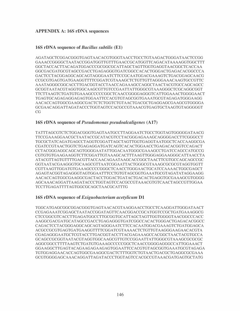
146
APPENDIX A: 16S rDNA sequences
16S rDNA sequence of Bacillus subtilis (E1) AGATAGCTCGGACGGGTGAGTAACACGTGGGTAACCTGCCTGTAAGACTGGGATAACTCCGGGAAACCGGGGCTAATACCGGATGGTTGTTTGAACCGCATGGTTCAGACATAAAAGGTGGCTTTGGCTACCACTTACAGATGGACCCGCGGCGCATTAGCTAGTTGGTGAGGTAACGGCTCACCAAGGCGACGATGCGTAGCCGACCTGAGAGGGTGATCGGCCACACTGGGACTGAGACACGGCCCAGACTCCTACGGAGGCAGCAGTAGGGAATCTTCCGCAATGGACGAAAGTCTGACGGAGCAACGCCGCGTGAGTGATGAAGGTTTTCGGATCGTAAAGCTCTGTTGTTAGGGAAACAAGTGCCGTTCAAATAGGGCGGCACCTTGACGGTACCTAACCAGAAAGCCAGGCTAACTACGTGCCAGCAGCCGCGGTAATACGTAGGTGGCAAGCGTTGTCCGAATTATTGGGCGTAAAGGGCTCGCAGGCGGTTTCTTAAGTCTGATGTGAAAGCCCCCGGCTCAACCGGGGAGGGTCATTGGAAACTGGGGAACTTGAGTGCAGAGAGGAGAGTGGAATTCCACGTGTAGCGGTGAAATGCGTAGAGATGGGAAGGAACACCAGTGGCGAAGGCGACTCTCTGGTCTGTAACTGACGCTGAGGAGCGAAGCGTGGGGAGCGAACAGGATTAGATACCCTGGTAGTCCACGCCGTAAACGTGAGTGCTAAGTGTAGGGGGTCG 16S rDNA sequence of Pseudomonas pseudoalcaligenes (A17) TATTTAGCGTCTCTGGACGGGTGAGTAATGCCTTAGGAATCTGCCTGGTAGTGGGGGATAACGTTCCGAAAGGAACGCTAATACCGCATACGTCCTACGGGAGAAAGCAGGGGACCTTCGGGCCTTGCGCTATCAGATGAGCCTAGGTCGGATTAGCTAGTTGGTGAGGTAATGGCTCACCAAGGCGACGATCCGTAACTGGTCTGAGAGGATGATCAGTCACACTGGAACCTGAGACACGGTCCAGACTCCTACGGGAGGCAGCAGTGGGGAATATTGGACAATGGGCGAAAGCCTGATCCAGCCATGCCGCGTGTGTGAAGAAGGTCTTCGGATTGTAAAGCACTTTAAGTTGGGAGGAAGGGCATTAACCTAATACGTTAGTGTTTTGACGTTACCAACAGAATAAGCACCGGCTAACTTCGTGCCAGCAGCCGCGGTAATACGAAGGGTGCAAGCGTTAATCGGAATTACTGGGCGTAAAGCGCGCGTAGGTGGTTCGTTAAGTTGGATGTGAAAGCCCCGGGCTCAACCTGGGAACTGCATCCAAAACTGGCGAGCTAGAGTACGGTAGAGGGTAGTGGAATTTCCTGTGTAGCGGTGAAATGCGTAGATATAGGAAGGAACACCAGTGGCGAAGGCGACTACCTGGACTGATACTGACACTGAGGTGCGAAAGCGTGGGGAGCAAACAGGATTAAGATACCCTGGTAGTCCACGCCGTAAACGTGTCAACTAGCCGTTGGAATCCTTGAGATTTTAGTGGCGCAGCTAACGCATTTG 16S rDNA sequence of Exiguobacterium acetylicum D1 TGGCATGAGCGGCGGACGGGTGAGTAACACGTAAGGAACCTGCCTCAAGGATTGGGATAACTCCGAGAAATCGGAGCTAATACCGGATAGTTCAACGGACCGCATGGTCCGCTGATGAAAGGCGCTCCGGCGTCACCTTGAGATGGCCTTGCGGTGCATTAGCTAGTTGGTGGGGTAACGGCCCACCAAGGCGACGATGCATAGCCGACCTGAGAGGGTGATCGGCCACACTGGGACTGAGACACGGCCCAGACTCCTACGGGAGGCAGCAGTAGGGAATCTTCCACAATGGACGAAAGTCTGATGGAGCAACGCCGCGTGAGTGATGAAGGTTTTCGGATCGTAAAACTCTGTTGTAAGGGAAGAACACGTACGAGAGGGAATGCTCGTACCTTGACGGTACCTTACGAGAAAGCCACGGCTAACTACGTGCCAGCAGCCGCGGTAATACGTAGGTGGCAAGCGTTGTCCGGAATTATTGGGCGTAAAGCGCGCGCAGGCGGCCTTTTAAGTCTGATGTGAAAGCCCCCGGCTCAACCGGGGAGGGCCATTGGAAACTGGAAGGCTTGAGTACAGAAGAGAAGAGTGGAATTCCACGTGTAGCGGTGAAATGCGTAGAGATGTGGAGGAACACCAGTGGCGAAGGCGACTCTTTGGTCTGTAACTGACGCTGAGGCGCGAAAGCGTGGGGAGCAAACAGGATTAGATACCCTGGTAGTCCACGCCGTAAACGATGAGTGCTATG
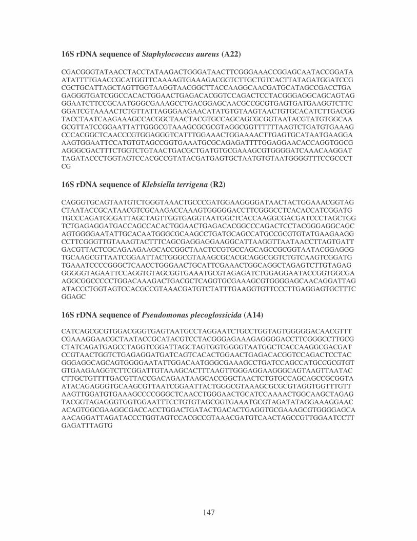
147
16S rDNA sequence of Staphylococcus aureus (A22) CGACGGGTATAACCTACCTATAAGACTGGGATAACTTCGGGAAACCGGAGCAATACCGGATAATATTTTGAACCGCATGGTTCAAAAGTGAAAGACGGTCTTGCTGTCACTTATAGATGGATCCGCGCTGCATTAGCTAGTTGGTAAGGTAACGGCTTACCAAGGCAACGATGCATAGCCGACCTGAGAGGGTGATCGGCCACACTGGAACTGAGACACGGTCCAGACTCCTACGGGAGGCAGCAGTAGGGAATCTTCCGCAATGGGCGAAAGCCTGACGGAGCAACGCCGCGTGAGTGATGAAGGTCTTCGGATCGTAAAACTCTGTTATTAGGGAAGAACATATGTGTAAGTAACTGTGCACATCTTGACGGTACCTAATCAAGAAAGCCACGGCTAACTACGTGCCAGCAGCGCGGTAATACGTATGTGGCAAGCGTTATCCGGAATTATTGGGCGTAAAGCGCGCGTAGGCGGTTTTTTAAGTCTGATGTGAAAGCCCACGGCTCAACCCGTGGAGGGTCATTTGGAAACTGGAAAACTTGAGTGCATAATGAAGGAAAGTGGAATTCCATGTGTAGCCGGTGAAATGCGCAGAGATTTTGGAGGAACACCAGGTGGCGAGGGCGACTTTCTGGTCTGTAACTGACGCTGATGTGCGAAAGCGTGGGGATCAAACAAGGATTAGATACCCTGGTAGTCCACGCCGTATACGATGAGTGCTAATGTGTAATGGGGTTTCCGCCCTCG 16S rDNA sequence of Klebsiella terrigena (R2) CAGGGTGCAGTAATGTCTGGGTAAACTGCCCGATGGAAGGGGATAACTACTGGAAACGGTAGCTAATACCGCATAACGTCGCAAGACCAAAGTGGGGGACCTTCGGGCCTCACACCATCGGATGTGCCCAGATGGGATTAGCTAGTTGGTGAGGTAATGGCTCACCAAGGCGACGATCCCTAGCTGGTCTGAGAGGATGACCAGCCACACTGGAACTGAGACACGGCCCAGACTCCTACGGGAGGCAGCAGTGGGGAATATTGCACAATGGGCGCAAGCCTGATGCAGCCATGCCGCGTGTATGAAGAAGGCCTTCGGGTTGTAAAGTACTTTCAGCGAGGAGGAAGGCATTAAGGTTAATAACCTTAGTGATTGACGTTACTCGCAGAAGAAGCACCGGCTAACTCCGTGCCAGCAGCCGCGGTAATACGGAGGGTGCAAGCGTTAATCGGAATTACTGGGCGTAAAGCGCACGCAGGCGGTCTGTCAAGTCGGATGTGAAATCCCCGGGCTCAACCTGGGAACTGCATTCGAAACTGGCAGGCTAGAGTCTTGTAGAGGGGGGTAGAATTCCAGGTGTAGCGGTGAAATGCGTAGAGATCTGGAGGAATACCGGTGGCGAAGGCGGCCCCCTGGACAAAGACTGACGCTCAGGTGCGAAAGCGTGGGGAGCAACAGGATTAGATACCCTGGTAGTCCACGCCGTAAACGATGTCTATTTGAAGGTGTTCCCTTGAGGAGTGCTTTCGGAGC 16S rDNA sequence of Pseudomonas plecoglossicida (A14) CATCAGCGCGTGGACGGGTGAGTAATGCCTAGGAATCTGCCTGGTAGTGGGGGACAACGTTTCGAAAGGAACGCTAATACCGCATACGTCCTACGGGAGAAAGAGGGGACCTTCGGGCCTTGCGCTATCAGATGAGCCTAGGTCGGATTAGCTAGTGGTGGGGTAATGGCTCACCAAGGCGACGATCCGTAACTGGTCTGAGAGGATGATCAGTCACACTGGAACTGAGACACGGTCCAGACTCCTACGGGAGGCAGCAGTGGGGAATATTGGACAATGGGCGAAAGCCTGATCCAGCCATGCCGCGTGTGTGAAGAAGGTCTTCGGATTGTAAAGCACTTTAAGTTGGGAGGAAGGGCAGTAAGTTAATACCTTGCTGTTTTGACGTTACCGACAGAATAAGCACCGGCTAACTCTGTGCCAGCAGCCGCGGTAATACAGAGGGTGCAAGCGTTAATCGGAATTACTGGGCGTAAAGCGCGCGTAGGTGGTTTGTTAAGTTGGATGTGAAAGCCCCGGGCTCAACCTGGGAACTGCATCCAAAACTGGCAAGCTAGAGTACGGTAGAGGGTGGTGGAATTTCCTGTGTAGCGGTGAAATGCGTAGATATAGGAAAGGAACACAGTGGCGAAGGCGACCACCTGGACTGATACTGACACTGAGGTGCGAAAGCGTGGGGAGCAAACAGGATTAGATACCCTGGTAGTCCACGCCGTAAACGATGTCAACTAGCCGTTGGAATCCTTGAGATTTAGTG
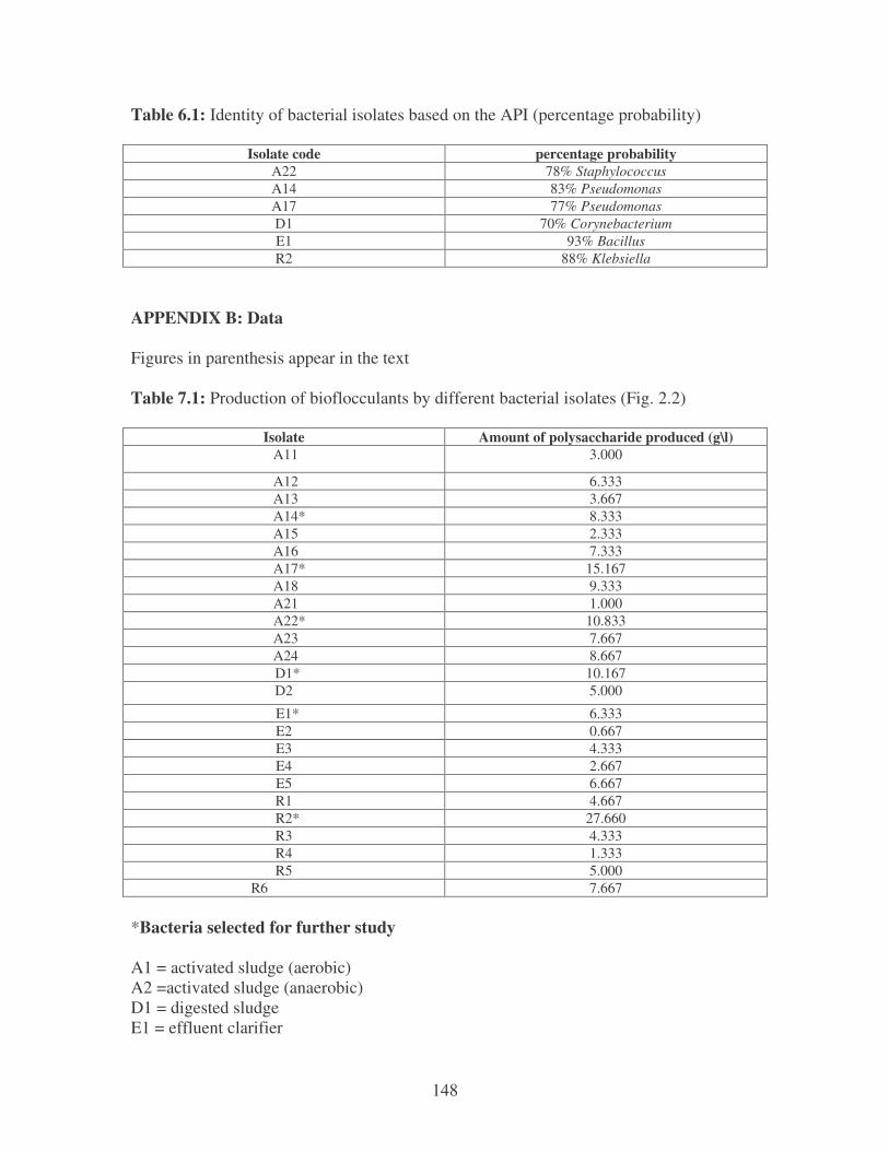
148
Table 6.1: Identity of bacterial isolates based on the API (percentage probability)
Isolate code percentage probability A22 78% Staphylococcus A14 83% Pseudomonas A17 77% Pseudomonas D1 70% Corynebacterium E1 93% Bacillus R2 88% Klebsiella
APPENDIX B: Data Figures in parenthesis appear in the text Table 7.1: Production of bioflocculants by different bacterial isolates (Fig. 2.2)
Isolate Amount of polysaccharide produced (g\l) A11 3.000
A12 6.333 A13 3.667
A14* 8.333 A15 2.333 A16 7.333
A17* 15.167 A18 9.333 A21 1.000
A22* 10.833 A23 7.667 A24 8.667 D1* 10.167 D2 5.000
E1* 6.333 E2 0.667 E3 4.333 E4 2.667 E5 6.667 R1 4.667
R2* 27.660 R3 4.333 R4 1.333 R5 5.000
R6 7.667 *Bacteria selected for further study A1 = activated sludge (aerobic) A2 =activated sludge (anaerobic) D1 = digested sludge E1 = effluent clarifier

149
(a) Phenol-sulfuric acid assay for the determination of carbohydrates
Sensitivity: glucose (0.05−2mM)
Final volume: 1.4 ml
Reagents:
(a) phenol dissolved in water (5% w/v).
(b) Concentrated sulphuric acid.
Method
(i) Mix samples, standards and control solutions (200 µl containing up to 100 µg
carbohydrate) with 200 µl of reagent A.
(ii) Add 1.0 ml of reagent B rapidly and directly to the solution surface without
touching the sides of the tube.
(iii) Leave the solutions undisturbed for 10 min before shaking vigorously.
(iv) Determine the absorbance at 490 nm after a further 30 min.
(b) Folin-Lowry method for the determination of protein
Sensitivity: Bovine serum albumin (0.002−2.000mM)
Final volume: 6.5 ml
Reagents:
(a) 2% Na2CO3 in 0.1 N NaOH
(b) 1% NaK Tartrate in H2O
(c) 0.5% CuSO4.5 H2O in H2O
(d) 48 ml of A, 1 ml of B, 1 ml C
(e) Phenol Reagent − 1 part Folin-Phenol (2 N): 1 part water
Method
(i) Add 5 ml of reagent D to 1 ml of the test solution.
(ii) Mix thoroughly and allow to stand for 10 min or longer.
(iii) Add 0.5 ml of reagent E rapidly with immediate mixing.
(iv) After 30 min read the extinction against the appropriate blank at 750 nm
150
(v) Estimate the protein concentration of the unknown solution after preparing a
standard curve.
(c) Carbazole assay for the determination of uronic acid
Sensitivity: D-glucurono-6,3-lactone (0.001−0.050mM)
Final volume: 1.8 ml
Reagents:
(a) Dissolve 0.95 g of sodium tetraborate decahydrates in 2.0 ml of hot water and add
98 ml of ice-cold concentrated sulphuric acid carefully with stirring.
(b) Dissolve 125 mg of carbazole (recrystallized from ethanol) in 100 ml of absolute
ethanol to give a stable reagent.
Method
(i) Cool the samples, standards and controls (250 µl) in an ice bath.
(ii) Add ice-cold reagent A (1.5 ml) with mixing and cooling in the ice bath.
(iii) Heat the mixtures at 100oC for 10 min.
(iv) Cool rapidly in the ice-bath.
(v) Add 50 µl of reagent B and mix well.
(vi) Reheat at 100oC for 15 min.
(vii) Cool rapidly at room temperature and determine the absorbance at 525 nm.
(d) Morgan–Elson assay for the determination of hexosamine
Sensitivity: 2-acetamido-2-deoxy-D-glucose(0.001−0.110 mM)
Final volume: 1.8 ml
Reagents:
(a) Dissolve 6.1 g of di-potassium tetraborate tetrahydrate in 80 ml of water and
make up to 100 ml with water.
(b) Add 1.5 ml of water to 11 ml of concentrated hydrochloric acid. Add a further
87.5 ml of glacial acetic acid and dissolve 10 g of 4-(N,N-dimethylamino)-
151
benzaldehyde in this mixture. Dilute 10 ml to 100 ml with glacial acetic acid
immediately prior to use.
Method
(i) Add samples, standards and controls (250 µl) to 50 µl of reagent A
(ii) Heat each mixture at 100oC for 3 min.
(iii) After cooling rapidly to room temperature, add 1.5 ml of reagent B, washing
down any condensate formed.
(iv) Incubate the samples at 37oC for 20 min.
(v) After cooling to room temperature, determine the absorbance at 585 nm.
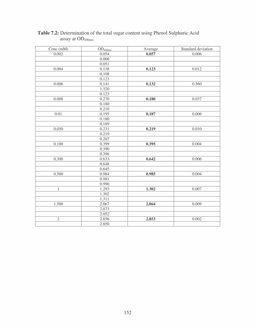
152
Table 7.2: Determination of the total sugar content using Phenol Sulphuric Acid assay at OD490nm
Conc (mM) OD490nm Average Standard deviation 0.002 0.054 0.057 0.006
0.066 0.051
0.004 0.138 0.123 0.012 0.108 0.123
0.006 0.141 0.132 0.560 1.320 0.123
0.008 0.270 0.180 0.037 0.180 0.210
0.01 0.195 0.187 0.006 0.180 0.189
0.050 0.231 0.219 0.010 0.219 0.207
0.100 0.399 0.395 0.004 0.390 0.396
0.300 0.633 0.642 0.006 0.648 0.645
0.500 0.984 0.985 0.004 0.981 0.990
1 1.293 1.302 0.007 1.302 1.311
1.500 2.067 2.064 0.009 2.073 2.052
2 2.856 2.853 0.002 2.850
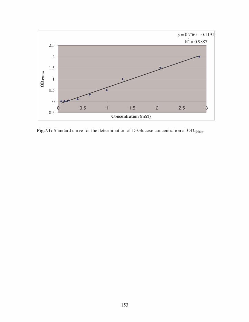
153
y = 0.756x - 0.1191
R2 = 0.9887
-0.5
0
0.5
1
1.5
2
2.5
0 0.5 1 1.5 2 2.5 3
Concentration (mM)
OD
490n
m
Fig.7.1: Standard curve for the determination of D-Glucose concentration at OD490nm.
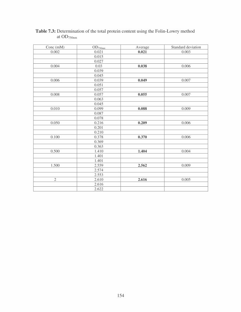
154
Table 7.3: Determination of the total protein content using the Folin-Lowry method at OD750nm
Conc (mM) OD750nm Average Standard deviation
0.002 0.021 0.021 0.003 0.015 0.027
0.004 0.03 0.038 0.006 0.039 0.045
0.006 0.039 0.049 0.007 0.051 0.057
0.008 0.057 0.055 0.007 0.063 0.045
0.010 0.099 0.088 0.009 0.087 0.078
0.050 0.216 0.209 0.006 0.201 0.210
0.100 0.378 0.370 0.006 0.369 0.363
0.500 1.410 1.404 0.004 1.401 1.401
1.500 2.559 2.562 0.009 2.574 2.553
2 2.610 2.616 0.005 2.616 2.622
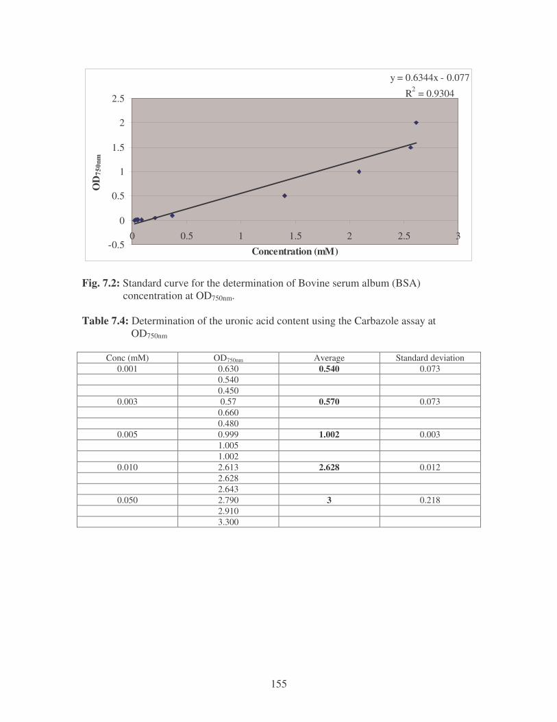
155
y = 0.6344x - 0.077
R2 = 0.9304
-0.5
0
0.5
1
1.5
2
2.5
0 0.5 1 1.5 2 2.5 3
Concentration (mM)
OD
750n
m
Fig. 7.2: Standard curve for the determination of Bovine serum album (BSA) concentration at OD750nm. Table 7.4: Determination of the uronic acid content using the Carbazole assay at OD750nm
Conc (mM) OD750nm Average Standard deviation
0.001 0.630 0.540 0.073 0.540 0.450
0.003 0.57 0.570 0.073 0.660 0.480
0.005 0.999 1.002 0.003 1.005 1.002
0.010 2.613 2.628 0.012 2.628 2.643
0.050 2.790 3 0.218 2.910 3.300
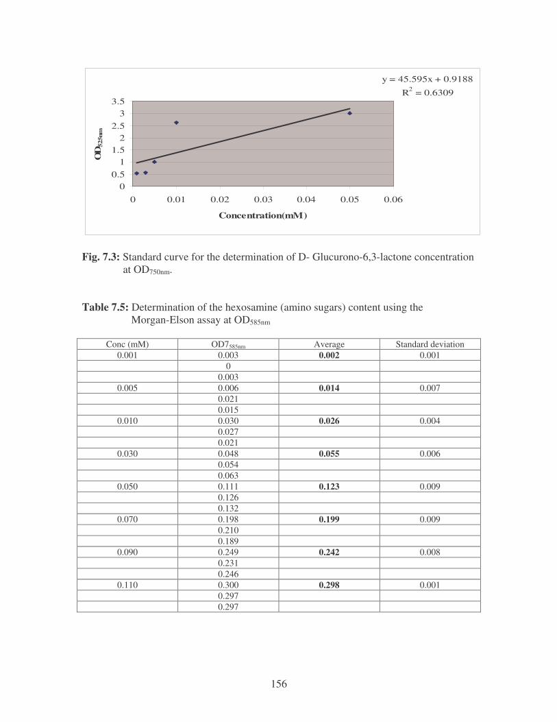
156
y = 45.595x + 0.9188
R2 = 0.6309
00.5
11.5
22.5
33.5
0 0.01 0.02 0.03 0.04 0.05 0.06
Concentration(mM)
OD
525n
m
Fig. 7.3: Standard curve for the determination of D- Glucurono-6,3-lactone concentration at OD750nm. Table 7.5: Determination of the hexosamine (amino sugars) content using the Morgan-Elson assay at OD585nm
Conc (mM) OD7585nm Average Standard deviation 0.001 0.003 0.002 0.001
0 0.003
0.005 0.006 0.014 0.007 0.021 0.015
0.010 0.030 0.026 0.004 0.027 0.021
0.030 0.048 0.055 0.006 0.054 0.063
0.050 0.111 0.123 0.009 0.126 0.132
0.070 0.198 0.199 0.009 0.210 0.189
0.090 0.249 0.242 0.008 0.231 0.246
0.110 0.300 0.298 0.001 0.297 0.297
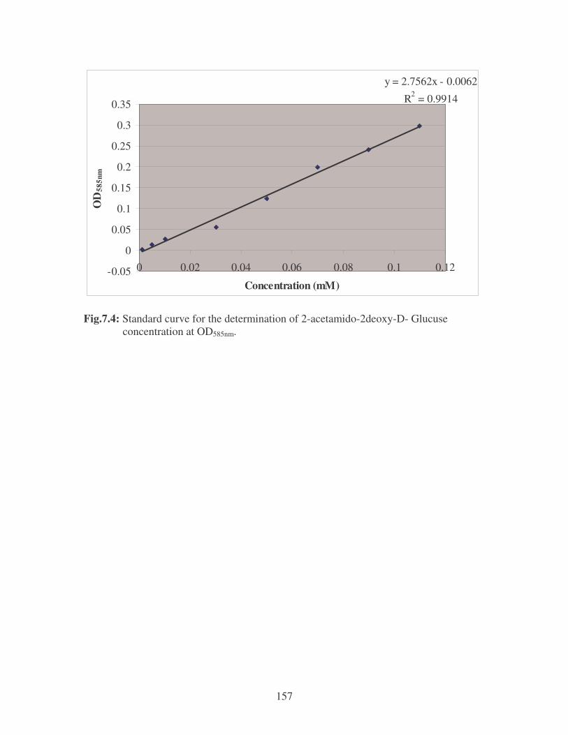
157
y = 2.7562x - 0.0062
R2 = 0.9914
-0.05
0
0.05
0.1
0.15
0.2
0.25
0.3
0.35
0 0.02 0.04 0.06 0.08 0.1 0.12
Concentration (mM)
OD
585n
m
Fig.7.4: Standard curve for the determination of 2-acetamido-2deoxy-D- Glucuse concentration at OD585nm.
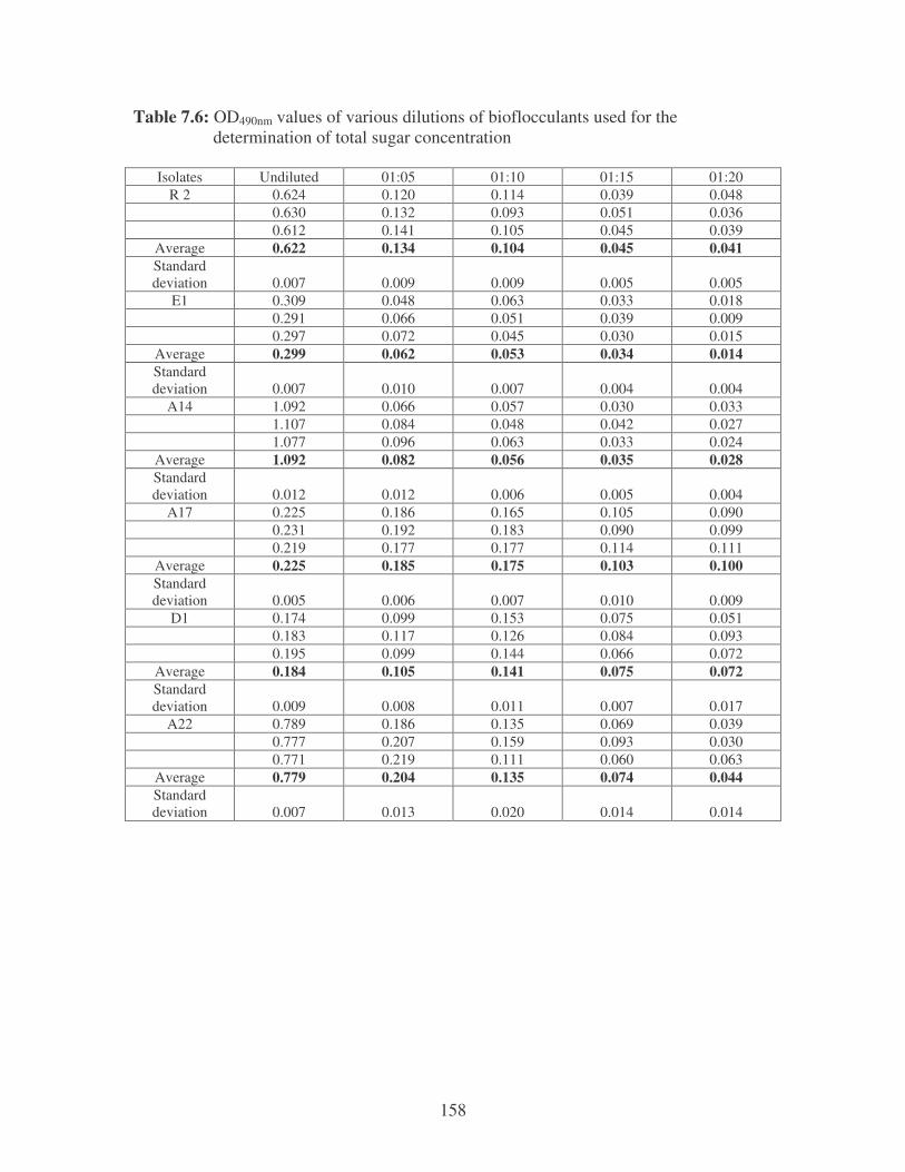
158
Table 7.6: OD490nm values of various dilutions of bioflocculants used for the determination of total sugar concentration
Isolates Undiluted 01:05 01:10 01:15 01:20 R 2 0.624 0.120 0.114 0.039 0.048
0.630 0.132 0.093 0.051 0.036 0.612 0.141 0.105 0.045 0.039
Average 0.622 0.134 0.104 0.045 0.041 Standard deviation 0.007 0.009 0.009 0.005 0.005
E1 0.309 0.048 0.063 0.033 0.018 0.291 0.066 0.051 0.039 0.009 0.297 0.072 0.045 0.030 0.015
Average 0.299 0.062 0.053 0.034 0.014 Standard deviation 0.007 0.010 0.007 0.004 0.004
A14 1.092 0.066 0.057 0.030 0.033 1.107 0.084 0.048 0.042 0.027 1.077 0.096 0.063 0.033 0.024
Average 1.092 0.082 0.056 0.035 0.028 Standard deviation 0.012 0.012 0.006 0.005 0.004
A17 0.225 0.186 0.165 0.105 0.090 0.231 0.192 0.183 0.090 0.099 0.219 0.177 0.177 0.114 0.111
Average 0.225 0.185 0.175 0.103 0.100 Standard deviation 0.005 0.006 0.007 0.010 0.009
D1 0.174 0.099 0.153 0.075 0.051 0.183 0.117 0.126 0.084 0.093 0.195 0.099 0.144 0.066 0.072
Average 0.184 0.105 0.141 0.075 0.072 Standard deviation 0.009 0.008 0.011 0.007 0.017
A22 0.789 0.186 0.135 0.069 0.039 0.777 0.207 0.159 0.093 0.030 0.771 0.219 0.111 0.060 0.063
Average 0.779 0.204 0.135 0.074 0.044 Standard deviation 0.007 0.013 0.020 0.014 0.014
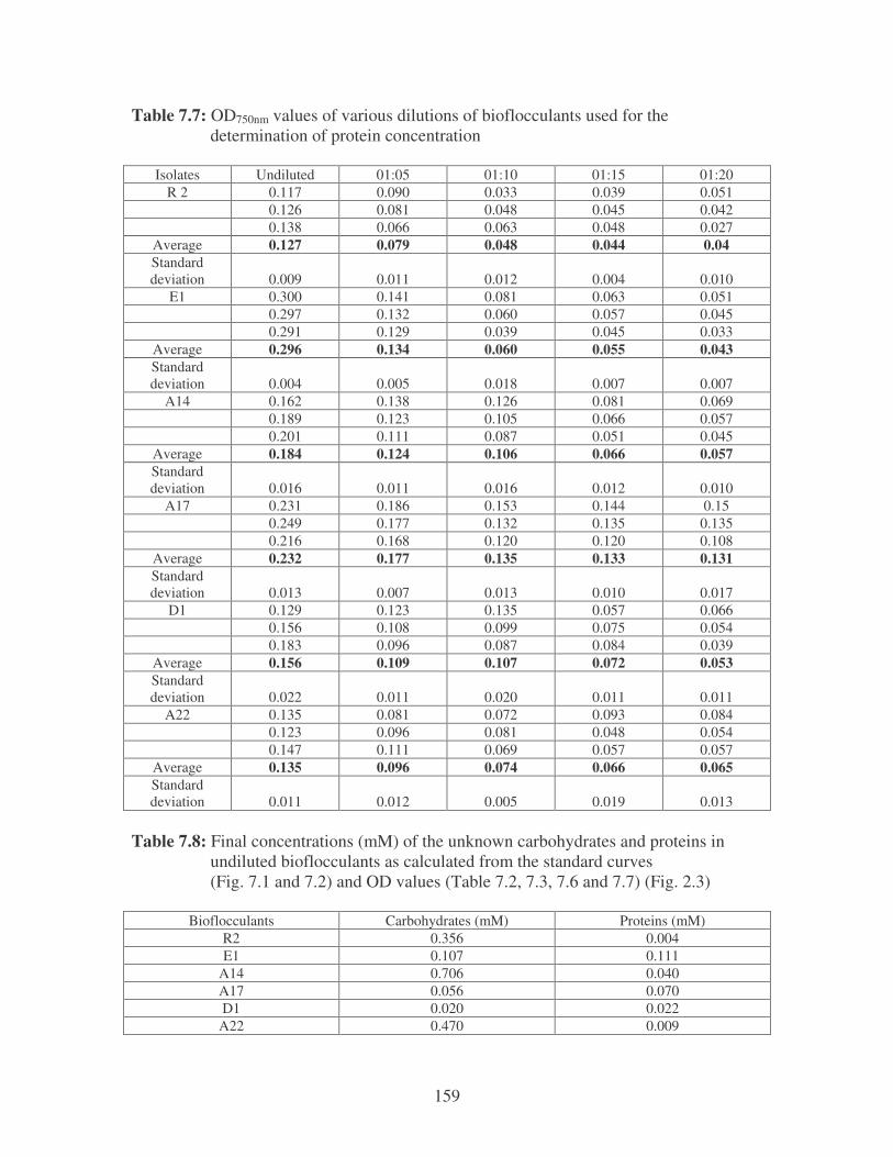
159
Table 7.7: OD750nm values of various dilutions of bioflocculants used for the determination of protein concentration
Isolates Undiluted 01:05 01:10 01:15 01:20 R 2 0.117 0.090 0.033 0.039 0.051
0.126 0.081 0.048 0.045 0.042 0.138 0.066 0.063 0.048 0.027
Average 0.127 0.079 0.048 0.044 0.04 Standard deviation 0.009 0.011 0.012 0.004 0.010
E1 0.300 0.141 0.081 0.063 0.051 0.297 0.132 0.060 0.057 0.045 0.291 0.129 0.039 0.045 0.033
Average 0.296 0.134 0.060 0.055 0.043 Standard deviation 0.004 0.005 0.018 0.007 0.007
A14 0.162 0.138 0.126 0.081 0.069 0.189 0.123 0.105 0.066 0.057 0.201 0.111 0.087 0.051 0.045
Average 0.184 0.124 0.106 0.066 0.057 Standard deviation 0.016 0.011 0.016 0.012 0.010
A17 0.231 0.186 0.153 0.144 0.15 0.249 0.177 0.132 0.135 0.135 0.216 0.168 0.120 0.120 0.108
Average 0.232 0.177 0.135 0.133 0.131 Standard deviation 0.013 0.007 0.013 0.010 0.017
D1 0.129 0.123 0.135 0.057 0.066 0.156 0.108 0.099 0.075 0.054 0.183 0.096 0.087 0.084 0.039
Average 0.156 0.109 0.107 0.072 0.053 Standard deviation 0.022 0.011 0.020 0.011 0.011
A22 0.135 0.081 0.072 0.093 0.084 0.123 0.096 0.081 0.048 0.054 0.147 0.111 0.069 0.057 0.057
Average 0.135 0.096 0.074 0.066 0.065 Standard deviation 0.011 0.012 0.005 0.019 0.013
Table 7.8: Final concentrations (mM) of the unknown carbohydrates and proteins in undiluted bioflocculants as calculated from the standard curves (Fig. 7.1 and 7.2) and OD values (Table 7.2, 7.3, 7.6 and 7.7) (Fig. 2.3)
Bioflocculants Carbohydrates (mM) Proteins (mM) R2 0.356 0.004 E1 0.107 0.111
A14 0.706 0.040 A17 0.056 0.070 D1 0.020 0.022 A22 0.470 0.009
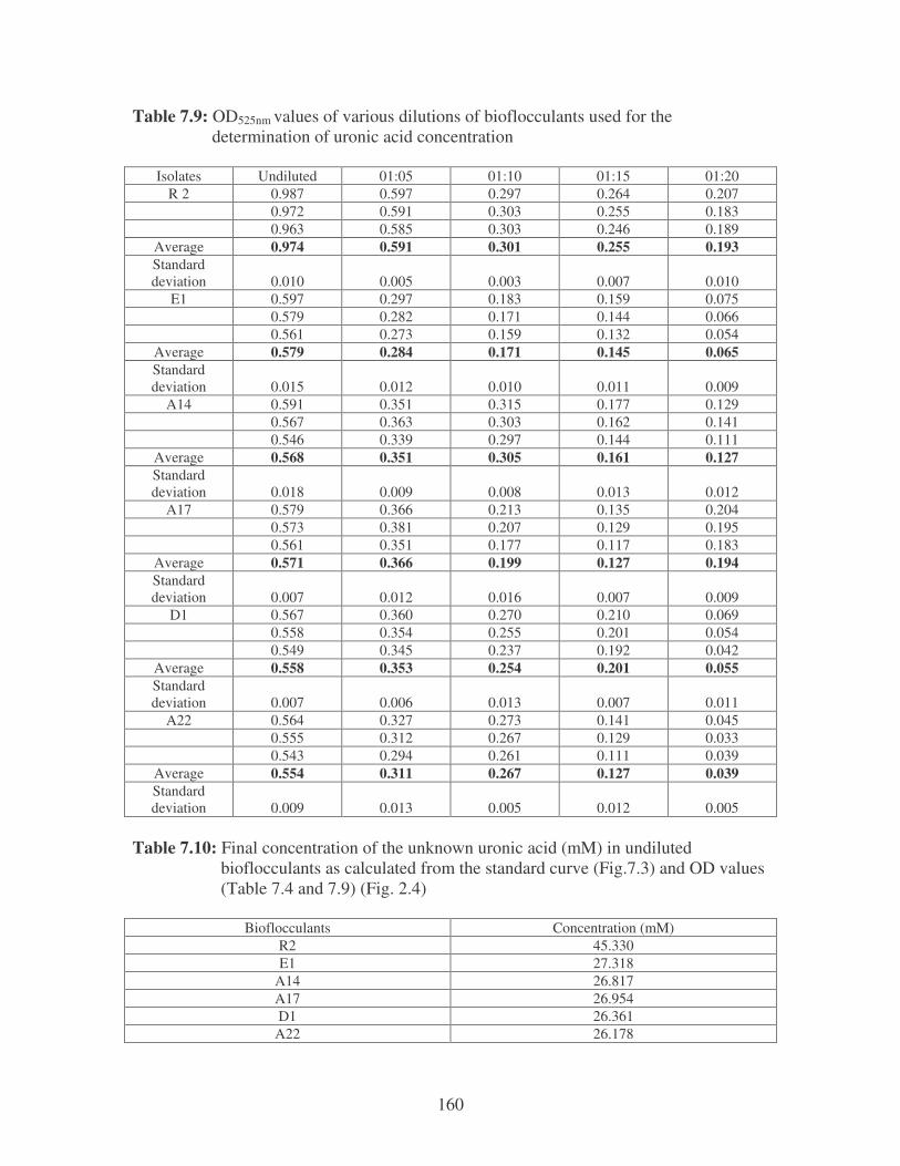
160
Table 7.9: OD525nm values of various dilutions of bioflocculants used for the determination of uronic acid concentration
Isolates Undiluted 01:05 01:10 01:15 01:20 R 2 0.987 0.597 0.297 0.264 0.207
0.972 0.591 0.303 0.255 0.183 0.963 0.585 0.303 0.246 0.189
Average 0.974 0.591 0.301 0.255 0.193 Standard deviation 0.010 0.005 0.003 0.007 0.010
E1 0.597 0.297 0.183 0.159 0.075 0.579 0.282 0.171 0.144 0.066 0.561 0.273 0.159 0.132 0.054
Average 0.579 0.284 0.171 0.145 0.065 Standard deviation 0.015 0.012 0.010 0.011 0.009
A14 0.591 0.351 0.315 0.177 0.129 0.567 0.363 0.303 0.162 0.141 0.546 0.339 0.297 0.144 0.111
Average 0.568 0.351 0.305 0.161 0.127 Standard deviation 0.018 0.009 0.008 0.013 0.012
A17 0.579 0.366 0.213 0.135 0.204 0.573 0.381 0.207 0.129 0.195 0.561 0.351 0.177 0.117 0.183
Average 0.571 0.366 0.199 0.127 0.194 Standard deviation 0.007 0.012 0.016 0.007 0.009
D1 0.567 0.360 0.270 0.210 0.069 0.558 0.354 0.255 0.201 0.054 0.549 0.345 0.237 0.192 0.042
Average 0.558 0.353 0.254 0.201 0.055 Standard deviation 0.007 0.006 0.013 0.007 0.011
A22 0.564 0.327 0.273 0.141 0.045 0.555 0.312 0.267 0.129 0.033 0.543 0.294 0.261 0.111 0.039
Average 0.554 0.311 0.267 0.127 0.039 Standard deviation 0.009 0.013 0.005 0.012 0.005
Table 7.10: Final concentration of the unknown uronic acid (mM) in undiluted bioflocculants as calculated from the standard curve (Fig.7.3) and OD values (Table 7.4 and 7.9) (Fig. 2.4)
Bioflocculants Concentration (mM) R2 45.330 E1 27.318
A14 26.817 A17 26.954 D1 26.361 A22 26.178
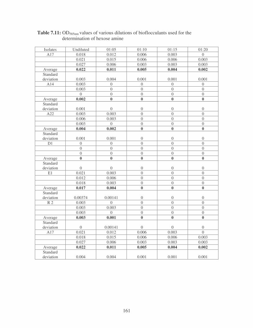
161
Table 7.11: OD585nm values of various dilutions of bioflocculants used for the determination of hexose amine
Isolates Undiluted 01:05 01:10 01:15 01:20 A17 0.018 0.012 0.006 0.003 0
0.021 0.015 0.006 0.006 0.003 0.027 0.006 0.003 0.003 0.003
Average 0.022 0.011 0.005 0.004 0.002 Standard deviation 0.003 0.004 0.001 0.001 0.001
A14 0.003 0 0 0 0 0.003 0 0 0 0 0 0 0 0 0
Average 0.002 0 0 0 0 Standard deviation 0.001 0 0 0 0
A22 0.003 0.003 0 0 0 0.006 0.003 0 0 0 0.003 0 0 0 0
Average 0.004 0.002 0 0 0 Standard deviation 0.001 0.001 0 0 0
D1 0 0 0 0 0 0 0 0 0 0 0 0 0 0 0
Average 0 0 0 0 0 Standard deviation 0 0 0 0 0
E1 0.021 0.003 0 0 0 0.012 0.006 0 0 0 0.018 0.003 0 0 0
Average 0.017 0.004 0 0 0 Standard deviation 0.00374 0.00141 0 0 0
R 2 0.003 0 0 0 0 0.003 0.003 0 0 0 0.003 0 0 0 0
Average 0.003 0.001 0 0 0 Standard deviation 0 0.00141 0 0 0
A17 0.021 0.012 0.006 0.003 0 0.018 0.015 0.006 0.006 0.003 0.027 0.006 0.003 0.003 0.003
Average 0.022 0.011 0.005 0.004 0.002 Standard deviation 0.004 0.004 0.001 0.001 0.001
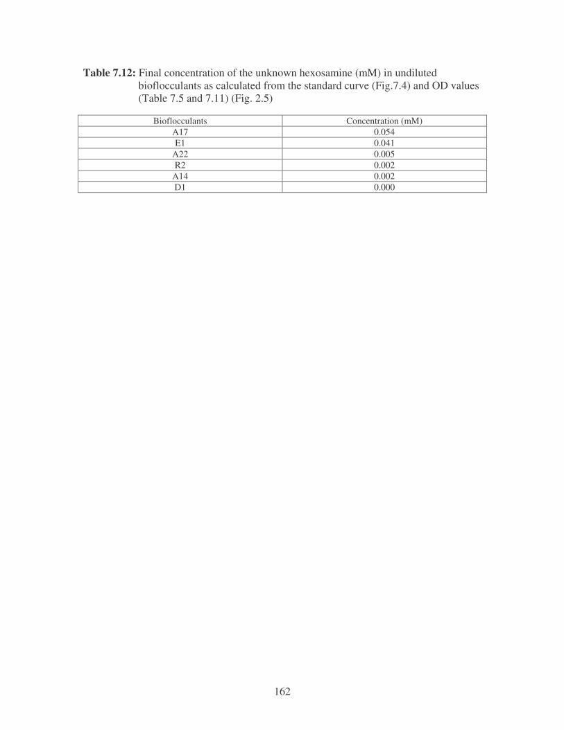
162
Table 7.12: Final concentration of the unknown hexosamine (mM) in undiluted bioflocculants as calculated from the standard curve (Fig.7.4) and OD values (Table 7.5 and 7.11) (Fig. 2.5)
Bioflocculants Concentration (mM) A17 0.054 E1 0.041
A22 0.005 R2 0.002
A14 0.002 D1 0.000
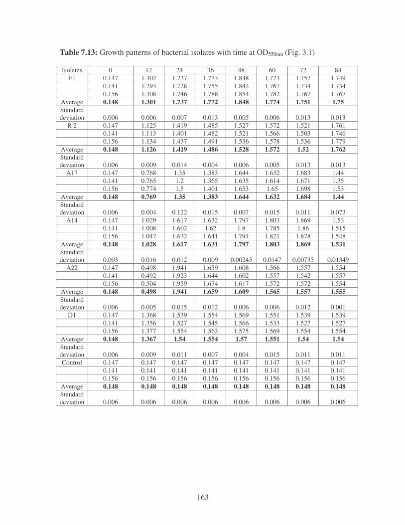
163
Table 7.13: Growth patterns of bacterial isolates with time at OD550nm (Fig. 3.1) Isolates 0 12 24 36 48 60 72 84
E1 0.147 1.302 1.737 1.773 1.848 1.773 1.752 1.749 0.141 1.293 1.728 1.755 1.842 1.767 1.734 1.734 0.156 1.308 1.746 1.788 1.854 1.782 1.767 1.767
Average 0.148 1.301 1.737 1.772 1.848 1.774 1.751 1.75 Standard deviation 0.006 0.006 0.007 0.013 0.005 0.006 0.013 0.013
R 2 0.147 1.125 1.419 1.485 1.527 1.572 1.521 1.761 0.141 1.113 1.401 1.482 1.521 1.566 1.503 1.746 0.156 1.134 1.437 1.491 1.536 1.578 1.536 1.779
Average 0.148 1.126 1.419 1.486 1.528 1.572 1.52 1.762 Standard deviation 0.006 0.009 0.014 0.004 0.006 0.005 0.013 0.013
A17 0.147 0.768 1.35 1.383 1.644 1.632 1.683 1.44 0.141 0.765 1.2 1.365 1.635 1.614 1.671 1.35 0.156 0.774 1.5 1.401 1.653 1.65 1.698 1.53
Average 0.148 0.769 1.35 1.383 1.644 1.632 1.684 1.44 Standard deviation 0.006 0.004 0.122 0.015 0.007 0.015 0.011 0.073
A14 0.147 1.029 1.617 1.632 1.797 1.803 1.869 1.53 0.141 1.008 1.602 1.62 1.8 1.785 1.86 1.515 0.156 1.047 1.632 1.641 1.794 1.821 1.878 1.548
Average 0.148 1.028 1.617 1.631 1.797 1.803 1.869 1.531 Standard deviation 0.003 0.016 0.012 0.009 0.00245 0.0147 0.00735 0.01349
A22 0.147 0.498 1.941 1.659 1.608 1.566 1.557 1.554 0.141 0.492 1.923 1.644 1.602 1.557 1.542 1.557 0.156 0.504 1.959 1.674 1.617 1.572 1.572 1.554
Average 0.148 0.498 1.941 1.659 1.609 1.565 1.557 1.555 Standard deviation 0.006 0.005 0.015 0.012 0.006 0.006 0.012 0.001
D1 0.147 1.368 1.539 1.554 1.569 1.551 1.539 1.539 0.141 1.356 1.527 1.545 1.566 1.533 1.527 1.527 0.156 1.377 1.554 1.563 1.575 1.569 1.554 1.554
Average 0.148 1.367 1.54 1.554 1.57 1.551 1.54 1.54 Standard deviation 0.006 0.009 0.011 0.007 0.004 0.015 0.011 0.011 Control 0.147 0.147 0.147 0.147 0.147 0.147 0.147 0.147
0.141 0.141 0.141 0.141 0.141 0.141 0.141 0.141 0.156 0.156 0.156 0.156 0.156 0.156 0.156 0.156
Average 0.148 0.148 0.148 0.148 0.148 0.148 0.148 0.148 Standard deviation 0.006 0.006 0.006 0.006 0.006 0.006 0.006 0.006

164
Table 7.14: OD550nm values at 12 hr time intervals for the determination of flocculating activity Isolates 0 12 24 36 48 60 72 84 E1 0.654 0.378 0.180 0.258 0.249 0.225 0.219 0.219 0.648 0.375 0.270 0.240 0.237 0.219 0.204 0.204 0.663 0.384 0.360 0.276 0.258 0.231 0.237 0.237 Average 0.655 0.379 0.270 0.258 0.248 0.225 0.220 0.220 Standard deviation 0.006 0.004 0.073 0.015 0.009 0.005 0.013 0.013 R 2 0.654 0.357 0.327 0.258 0.237 0.294 0.330 0.330 0.648 0.354 0.315 0.255 0.225 0.3 0.315 0.315 0.663 0.363 0.342 0.264 0.246 0.285 0.348 0.348 Average 0.655 0.358 0.328 0.259 0.236 0.293 0.331 0.331 Standard deviation 0.006 0.004 0.011 0.004 0.009 0.006 0.013 0.013 A17 0.654 0.480 0.192 0.273 0.309 0.315 0.324 0.324 0.648 0.390 0.177 0.252 0.291 0.306 0.318 0.318 0.663 0.570 0.104 0.291 0.324 0.321 0.333 0.333 Average 0.655 0.48 0.191 0.272 0.308 0.314 0.325 0.325 Standard deviation 0.006 0.073 0.038 0.016 0.013 0.006 0.006 0.006 A14 0.654 0.357 0.297 0.279 0.225 0.315 0.354 0.354 0.648 0.354 0.306 0.258 0.216 0.306 0.339 0.339 0.663 0.363 0.288 0.297 0.234 0.321 0.372 0.372 Average 0.655 0.538 0.297 0.278 0.225 0.314 0.355 0.355 Standard deviation 0.006 0.004 0.007 0.016 0.007 0.006 0.013 0.013 A22 0.654 0.576 0.273 0.219 0.219 0.330 0.333 0.333 0.648 0.567 0.252 0.204 0.201 0.330 0.321 0.321 0.663 0.585 0.291 0.237 0.234 0.360 0.348 0.348 Average 0.655 0.576 0.272 0.22 0.218 0.33 0.334 0.334 Standard deviation 0.006 0.007 0.015 0.013 0.013 0.014 0.011 0.011 D1 0.654 0.369 0.318 0.282 0.231 0.285 0.342 0.342 0.648 0.360 0.306 0.297 0.213 0.279 0.336 0.336 0.663 0.375 0.327 0.273 0.249 0.294 0.348 0.348 Average 0.655 0.368 0.317 0.284 0.231 0.286 0.342 0.342 Standard deviation 0.006 0.006 0.009 0.010 0.015 0.006 0.005 0.005 Control 0.654 0.654 0.654 0.654 0.654 0.654 0.654 0.654 0.648 0.648 0.648 0.648 0.648 0.648 0.648 0.648 0.663 0.663 0.663 0.663 0.663 0.663 0.663 0.663 Average 0.655 0.655 0.655 0.655 0.655 0.655 0.655 0.655 Standard deviation 0.006 0.006 0.006 0.006 0.006 0.006 0.006 0.006
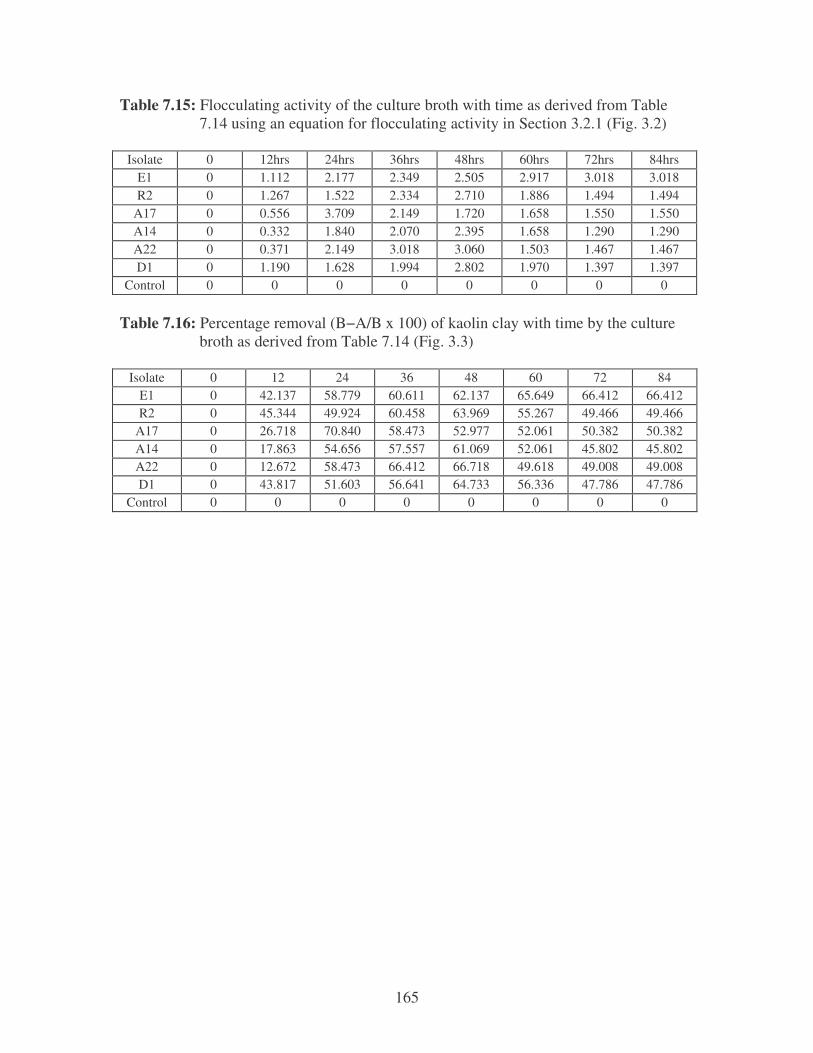
165
Table 7.15: Flocculating activity of the culture broth with time as derived from Table 7.14 using an equation for flocculating activity in Section 3.2.1 (Fig. 3.2)
Isolate 0 12hrs 24hrs 36hrs 48hrs 60hrs 72hrs 84hrs E1 0 1.112 2.177 2.349 2.505 2.917 3.018 3.018 R2 0 1.267 1.522 2.334 2.710 1.886 1.494 1.494
A17 0 0.556 3.709 2.149 1.720 1.658 1.550 1.550 A14 0 0.332 1.840 2.070 2.395 1.658 1.290 1.290 A22 0 0.371 2.149 3.018 3.060 1.503 1.467 1.467 D1 0 1.190 1.628 1.994 2.802 1.970 1.397 1.397
Control 0 0 0 0 0 0 0 0
Table 7.16: Percentage removal (B−A/B x 100) of kaolin clay with time by the culture broth as derived from Table 7.14 (Fig. 3.3)
Isolate 0 12 24 36 48 60 72 84 E1 0 42.137 58.779 60.611 62.137 65.649 66.412 66.412 R2 0 45.344 49.924 60.458 63.969 55.267 49.466 49.466
A17 0 26.718 70.840 58.473 52.977 52.061 50.382 50.382 A14 0 17.863 54.656 57.557 61.069 52.061 45.802 45.802 A22 0 12.672 58.473 66.412 66.718 49.618 49.008 49.008 D1 0 43.817 51.603 56.641 64.733 56.336 47.786 47.786
Control 0 0 0 0 0 0 0 0
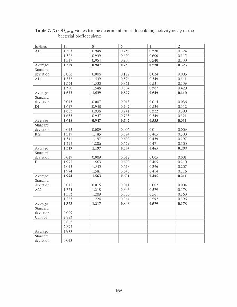
166
Table 7.17: OD550nm values for the determination of flocculating activity assay of the bacterial bioflocculants Isolates 10 8 6 4 2 A17 1.308 0.948 0.750 0.570 0.324 1.302 0.939 0.600 0.600 0.315 1.317 0.954 0.900 0.540 0.330 Average 1.309 0.947 0.75 0.570 0.323 Standard deviation 0.006 0.006 0.122 0.024 0.006 A14 1.572 1.539 0.876 0.549 0.411 1.554 1.530 0.861 0.531 0.339 1.590 1.548 0.894 0.567 0.420 Average 1.572 1.539 0.877 0.549 0.410 Standard deviation 0.015 0.007 0.013 0.015 0.036 D1 1.617 0.948 0.747 0.534 0.312 1.602 0.936 0.741 0.522 0.300 1.635 0.957 0.753 0.549 0.321 Average 1.618 0.947 0.747 0.535 0.311 Standard deviation 0.013 0.009 0.005 0.011 0.009 R 2 1.317 1.185 0.594 0.465 0.300 1.341 1.197 0.609 0.459 0.297 1.299 1.206 0.579 0.471 0.300 Average 1.319 1.197 0.594 0.465 0.299 Standard deviation 0.017 0.009 0.012 0.005 0.001 E1 1.995 1.563 0.630 0.405 0.210 2.013 1.545 0.618 0.396 0.207 1.974 1.581 0.645 0.414 0.216 Average 1.994 1.563 0.631 0.405 0.211 Standard deviation 0.015 0.015 0.011 0.007 0.004 A22 1.374 1.218 0.846 0.579 0.378 1.362 1.209 0.828 0.561 0.360 1.383 1.224 0.864 0.597 0.396 Average 1.373 1.217 0.846 0.579 0.378 Standard deviation 0.009 Control 2.883 2.862 2.892 Average 2.879 Standard deviation 0.013
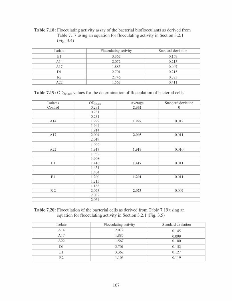
167
Table 7.18: Flocculating activity assay of the bacterial bioflocculants as derived from Table 7.17 using an equation for flocculating activity in Section 3.2.1 (Fig. 3.4)
Isolate Flocculating activity Standard deviation E1 3.362 0.159
A14 2.072 0.213 A17 1.885 0.407 D1 2.701 0.215 R2 2.746 0.383
A22 1.567 0.411 Table 7.19: OD550nm values for the determination of flocculation of bacterial cells
Isolates OD550nm Average Standard deviation Control 0.231 2.332 0
0.231 0.231
A14 1.929 1.929 0.012 1.944 1.914
A17 2.004 2.005 0.011 2.019 1.992
A22 1.917 1.919 0.010 1.932 1.908
D1 1.416 1.417 0.011 1.431 1.404
E1 1.200 1.201 0.011 1.215 1.188
R 2 2.073 2.073 0.007 2.082 2.064
Table 7.20: Flocculation of the bacterial cells as derived from Table 7.19 using an equation for flocculating activity in Section 3.2.1 (Fig. 3.5)
Isolate Flocculating activity Standard deviation A14 2.072 0.145 A17 1.885 0.099 A22 1.567 0.100
D1 2.701 0.152 E1 3.362 0.127 R2 1.103 0.119
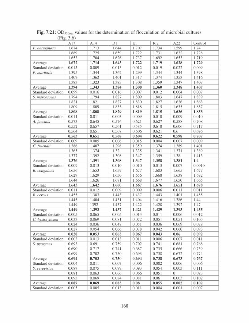
168
Fig. 7.21: OD550nm values for the determination of flocculation of microbial cultures (Fig. 3.6)
A17 A14 D1 E1 R 2 A22 Control P. aeruginosa 1.674 1.713 1.644 1.707 1.734 1.599 1.74 1.689 1.725 1.659 1.722 1.731 1.632 1.728 1.653 1.704 1.626 1.737 1.692 1.653 1.719 Average 1.672 1.714 1.643 1.722 1.719 1.628 1.729 Standard deviation 0.015 0.009 0.013 0.012 0.019 0.022 0.009 P. maribilis 1.395 1.344 1.362 1.299 1.344 1.344 1.398 1.407 1.362 1.401 1.317 1.374 1.353 1.416 1.383 1.323 1.383 1.308 1.359 1.347 1.407 Average 1.394 1.343 1.384 1.308 1.360 1.348 1.407 Standard deviation 0.099 0.016 0.016 0.007 0.012 0.004 0.007 S. marcescens 1.794 1.794 1.827 1.809 1.803 1.647 1.839 1.821 1.821 1.827 1.830 1.827 1.626 1.863 1.809 1.809 1.833 1.818 1.815 1.635 1.857 Average 1.808 1.808 1.829 1.819 1.815 1.636 1.853 Standard deviation 0.011 0.011 0.003 0.009 0.010 0.009 0.010 A. faecalis 0.573 0.645 0.576 0.621 0.627 0.588 0.708 0.552 0.657 0.561 0.585 0.618 0.606 0.717 0.564 0.651 0.567 0.606 0.621 0.6 0.696 Average 0.563 0.651 0.568 0.604 0.622 0.598 0.707 Standard deviation 0.009 0.005 0.006 0.015 0.004 0.007 0.009 C. fruendii 1.386 1.407 1.296 1.359 1.374 1.389 1.401 1.365 1.374 1.32 1.335 1.341 1.371 1.389 1.377 1.392 1.308 1.347 1.359 1.38 1.413 Average 1.376 1.391 1.308 1.347 1.358 1.381 1.4 Standard deviation 0.009 0.013 0.010 0.010 0.013 0.007 0.0010 B. coagulans 1.656 1.653 1.659 1.677 1.683 1.665 1.677 1.629 1.629 1.650 1.656 1.668 1.638 1.692 1.644 1.626 1.671 1.668 1.677 1.650 1.665 Average 1.643 1.642 1.660 1.667 1.676 1.651 1.678 Standard deviation 0.011 0.012 0.009 0.009 0.006 0.011 0.011 B. cereus 1.455 1.383 1.443 1.437 1.443 1.401 1.455 1.443 1.404 1.431 1.404 1.416 1.386 1.44 1.449 1392 1.437 1.422 1.428 1.392 1.47 Average 1.449 1.393 1.437 1.421 1.429 1.393 1.455 Standard deviation 0.005 0.065 0.005 0.013 0.011 0.006 0.012 C. hystolyticum 0.033 0.069 0.081 0.072 0.051 0.051 0.105 0.024 0.036 0.048 0.051 0.036 0.069 0.078 0.027 0.054 0.066 0.078 0.042 0.060 0.093 Average 0.028 0.053 0.065 0.067 0.043 0.06 0.092 Standard deviation 0.003 0.013 0.013 0.011 0.006 0.007 0.011 S. pyogenes 0.693 0.69 0.759 0.702 0.741 0.681 0.768 0.690 0.717 0.741 0.687 0.735 0.666 0.759 0.699 0.702 0.750 0.693 0.738 0.672 0.774 Average 0.694 0.703 0.750 0.694 0.738 0.673 0.767 Standard deviation 0.004 0.011 0.007 0.006 0.002 0.006 0.006 S. cerevisiae 0.087 0.075 0.099 0.093 0.054 0.003 0.111 0.081 0.063 0.066 0.066 0.051 0 0.093 0.093 0.069 0.084 0.081 0.06 0.003 0.102 Average 0.087 0.069 0.083 0.08 0.055 0.002 0.102 Standard deviation 0.005 0.005 0.013 0.011 0.004 0.001 0.007
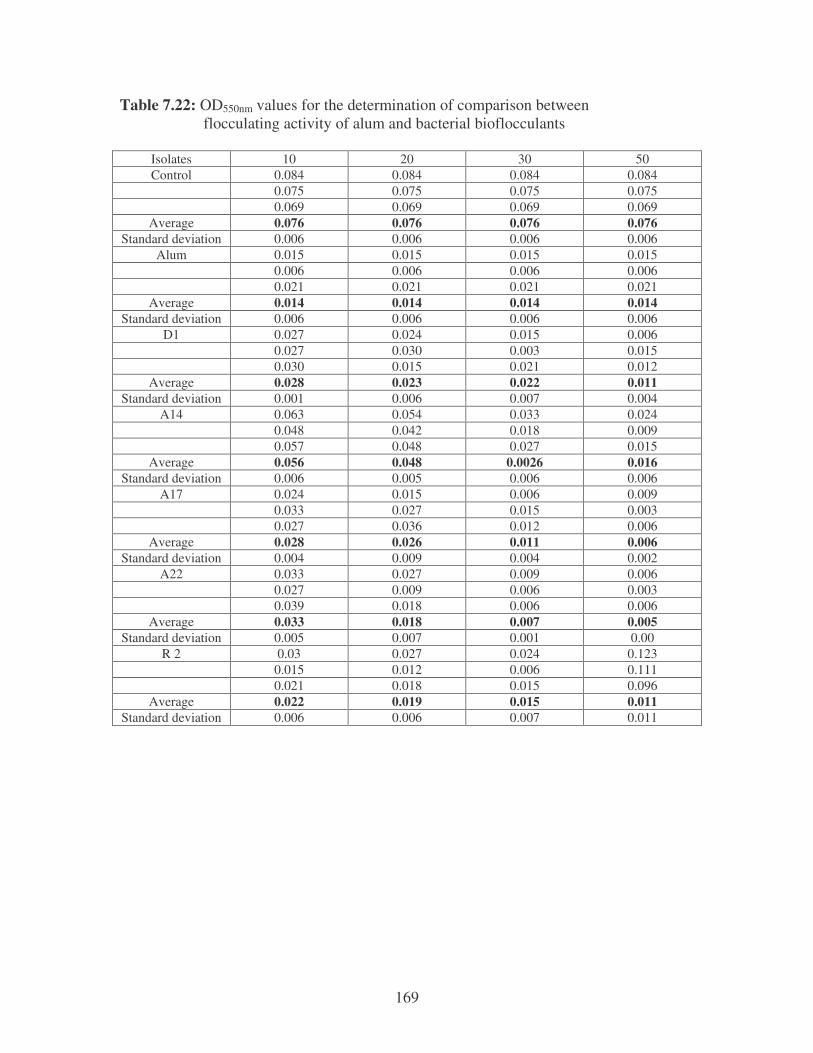
169
Table 7.22: OD550nm values for the determination of comparison between flocculating activity of alum and bacterial bioflocculants
Isolates 10 20 30 50 Control 0.084 0.084 0.084 0.084
0.075 0.075 0.075 0.075 0.069 0.069 0.069 0.069
Average 0.076 0.076 0.076 0.076 Standard deviation 0.006 0.006 0.006 0.006
Alum 0.015 0.015 0.015 0.015 0.006 0.006 0.006 0.006 0.021 0.021 0.021 0.021
Average 0.014 0.014 0.014 0.014 Standard deviation 0.006 0.006 0.006 0.006
D1 0.027 0.024 0.015 0.006 0.027 0.030 0.003 0.015 0.030 0.015 0.021 0.012
Average 0.028 0.023 0.022 0.011 Standard deviation 0.001 0.006 0.007 0.004
A14 0.063 0.054 0.033 0.024 0.048 0.042 0.018 0.009 0.057 0.048 0.027 0.015
Average 0.056 0.048 0.0026 0.016 Standard deviation 0.006 0.005 0.006 0.006
A17 0.024 0.015 0.006 0.009 0.033 0.027 0.015 0.003 0.027 0.036 0.012 0.006
Average 0.028 0.026 0.011 0.006 Standard deviation 0.004 0.009 0.004 0.002
A22 0.033 0.027 0.009 0.006 0.027 0.009 0.006 0.003 0.039 0.018 0.006 0.006
Average 0.033 0.018 0.007 0.005 Standard deviation 0.005 0.007 0.001 0.00
R 2 0.03 0.027 0.024 0.123 0.015 0.012 0.006 0.111 0.021 0.018 0.015 0.096
Average 0.022 0.019 0.015 0.011 Standard deviation 0.006 0.006 0.007 0.011
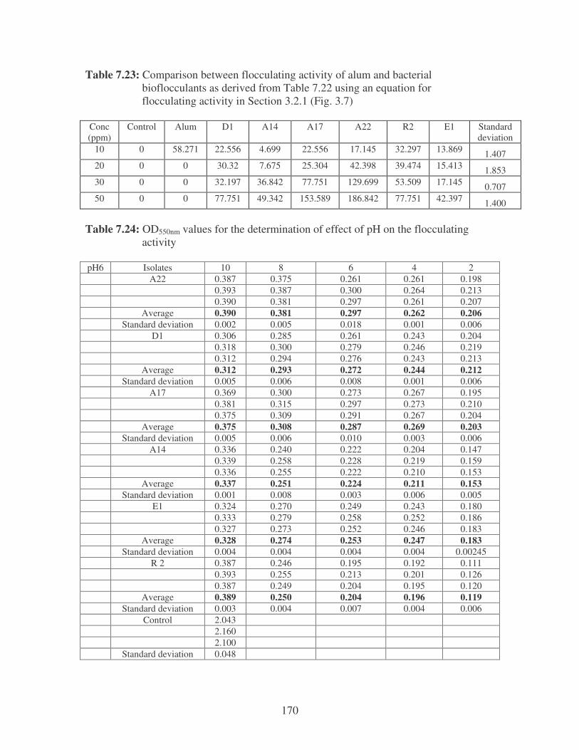
170
Table 7.23: Comparison between flocculating activity of alum and bacterial bioflocculants as derived from Table 7.22 using an equation for flocculating activity in Section 3.2.1 (Fig. 3.7) Conc (ppm)
Control Alum D1 A14 A17 A22 R2 E1 Standard deviation
10 0 58.271 22.556 4.699 22.556 17.145 32.297 13.869 1.407 20 0 0 30.32 7.675 25.304 42.398 39.474 15.413 1.853 30 0 0 32.197 36.842 77.751 129.699 53.509 17.145 0.707 50 0 0 77.751 49.342 153.589 186.842 77.751 42.397 1.400
Table 7.24: OD550nm values for the determination of effect of pH on the flocculating activity pH6 Isolates 10 8 6 4 2
A22 0.387 0.375 0.261 0.261 0.198 0.393 0.387 0.300 0.264 0.213 0.390 0.381 0.297 0.261 0.207 Average 0.390 0.381 0.297 0.262 0.206 Standard deviation 0.002 0.005 0.018 0.001 0.006 D1 0.306 0.285 0.261 0.243 0.204 0.318 0.300 0.279 0.246 0.219 0.312 0.294 0.276 0.243 0.213 Average 0.312 0.293 0.272 0.244 0.212 Standard deviation 0.005 0.006 0.008 0.001 0.006 A17 0.369 0.300 0.273 0.267 0.195 0.381 0.315 0.297 0.273 0.210 0.375 0.309 0.291 0.267 0.204 Average 0.375 0.308 0.287 0.269 0.203 Standard deviation 0.005 0.006 0.010 0.003 0.006 A14 0.336 0.240 0.222 0.204 0.147 0.339 0.258 0.228 0.219 0.159 0.336 0.255 0.222 0.210 0.153 Average 0.337 0.251 0.224 0.211 0.153 Standard deviation 0.001 0.008 0.003 0.006 0.005 E1 0.324 0.270 0.249 0.243 0.180 0.333 0.279 0.258 0.252 0.186 0.327 0.273 0.252 0.246 0.183 Average 0.328 0.274 0.253 0.247 0.183 Standard deviation 0.004 0.004 0.004 0.004 0.00245 R 2 0.387 0.246 0.195 0.192 0.111 0.393 0.255 0.213 0.201 0.126 0.387 0.249 0.204 0.195 0.120 Average 0.389 0.250 0.204 0.196 0.119 Standard deviation 0.003 0.004 0.007 0.004 0.006 Control 2.043 2.160 2.100 Standard deviation 0.048

171
pH7 Isolates 10 8 6 4 2 A22 0.366 0.297 0.261 0.249 0.201 0.375 0.285 0.267 0.252 0.207 0.357 0.27 0.258 0.246 0.198 Average 0.366 0.284 0.262 0.249 0.202 Standard
deviation 0.007 0.011 0.004 0.002 0.004 D1 0.330 0.249 0.237 0.225 0.126 0.342 0.252 0.246 0.228 0.123 0.321 0.246 0.228 0.222 0.132 Average 0.331 0.249 0.237 0.225 0.127 Standard
deviation 0.009 0.002 0.007 0.002 0.004 A17 0.357 0.339 0.261 0.213 0.171 0.354 0.33 0.255 0.195 0.162 0.366 0.333 0.270 0.228 0.177 Average 0.359 0.334 0.262 0.212 0.17 Standard
deviation 0.005 0.004 0.006 0.013 0.006 A14 0.357 0.333 0.261 0.213 0.171 0.354 0.318 0.255 0.195 0.162 0.366 0.351 0.270 0.228 0.177 Average 0.359 0.334 0.262 0.212 0.170 Standard
deviation 0.005 0.014 0.006 0.013 0.006 E1 0.327 0.318 0.294 0.228 0.216 0.309 0.306 0.291 0.216 0.201 0.342 0.33 0.297 0.237 0.231 Average 0.326 0.318 0.294 0.227 0.216 Standard
deviation 0.013 0.010 0.002 0.009 0.012 R 2 0.345 0.339 0.237 0.213 0.192 0.336 0.327 0.225 0.201 0.186 0.357 0.354 0.246 0.225 0.198 Average 0.346 0.34 0.236 0.213 0.192 Standard
deviation 0.009 0.011 0.009 0.010 0.005 Control 2.256 2.256 2.259 Average 2.257 Standard
deviation 0.001
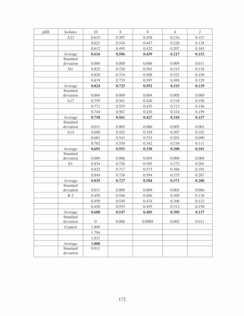
172
pH8 Isolates 10 8 6 4 2 A22 0.615 0.507 0.438 0.216 0.153 0.621 0.516 0.447 0.228 0.138 0.612 0.495 0.432 0.207 0.165 Average 0.616 0.506 0.439 0.217 0.152 Standard
deviation 0.004 0.009 0.006 0.009 0.011 D1 0.825 0.726 0.591 0.315 0.138 0.828 0.714 0.588 0.321 0.150 0.819 0.735 0.597 0.309 0.129 Average 0.824 0.725 0.592 0.315 0.139 Standard
deviation 0.004 0.009 0.004 0.005 0.009 A17 0.759 0.561 0.426 0.318 0.156 0.771 0.555 0.435 0.312 0.156 0.744 0.567 0.420 0.324 0.159 Average 0.758 0.561 0.427 0.318 0.157 Standard
deviation 0.011 0.005 0.006 0.005 0.001 A14 0.690 0.552 0.339 0.207 0.102 0.681 0.543 0.333 0.201 0.090 0.702 0.558 0.342 0.216 0.111 Average 0.691 0.551 0.338 0.208 0.101 Standard
deviation 0.009 0.006 0.004 0.006 0.009 E1 0.834 0.726 0.585 0.372 0.201 0.822 0.717 0.573 0.366 0.192 0.849 0.738 0.594 0.375 0.207 Average 0.835 0.727 0.584 0.371 0.200 Standard
deviation 0.011 0.009 0.009 0.004 0.006 R 2 0.450 0.546 0.486 0.309 0.138 0.450 0.540 0.474 0.306 0.123 0.450 0.555 0.495 0.312 0.150 Average 0.600 0.547 0.485 0.309 0.137 Standard
deviation 0 0.006 0.0089 0.002 0.011 Control 1.809 1.794 1.821 Average 1.808 Standard
deviation 0.011

173
pH9 Isolates 10 8 6 4 2 A22 0.891 0.684 0.513 0.423 0.255 0.885 0.675 0.504 0.411 0.252 0.897 0.690 0.519 0.435 0.261 Average 0.891 0.683 0.512 0.423 0.256 Standard
deviation 0.005 0.006 0.006 0.010 0.004 D1 0.714 0.627 0.588 0.414 0.222 0.711 0.621 0.582 0.408 0.219 0.741 0.633 0.597 0.423 0.228 Average 0.715 0.627 0.589 0.415 0.223 Standard
deviation 0.01 0.005 0.006 0.006 0.004 A17 0.873 0.723 0.618 0.405 0.210 0.855 0.717 0.612 0.399 0.201 0.888 0.729 0.627 0.408 0.222 Average 0.872 0.723 0.619 0.404 0.211 Standard
deviation 0.013 0.005 0.006 0.004 0.009 A14 0.918 0.783 0.630 0.573 0.234 0.912 0.783 0.624 0.561 0.222 0.927 0.780 0.639 0.582 0.249 Average 0.919 0.782 0.631 0.572 0.235 Standard
deviation 0.006 0.001 0.006 0.009 0.011 E1 0.657 0.567 0.405 0.216 0.138 0.648 0.564 0.408 0.207 0.129 0.69 0.576 0.399 0.225 0.147 Average 0.658 0.569 0.404 0.216 0.138 Standard
deviation 0.018 0.005 0.004 0.007 0.007 R 2 0.831 0.78 0.528 0.303 0.219 0.816 0.771 0.519 0.294 0.213 0.849 0.792 0.537 0.312 0.225 Average 0.832 0.781 0.528 0.303 0.219 Standard
deviation 0.014 0.009 0.007 0.007 0.005 Control 2.313 2.304 2.322 Average 2.313 Standard
deviation 0.007

174
pH10 Isolates 10 8 6 4 2 A22 0.825 0.684 0.438 0.216 0.159 0.813 0.675 0.432 0.204 0.156 0.834 0.690 0.447 0.225 0.156 Average 0.824 0.683 0.439 0.215 0.158 Standard
deviation 0.009 0.006 0.006 0.009 0.001 D1 0.765 0.675 0.531 0.357 0.210 0.753 0.669 0.525 0.348 0.195 0.777 0.678 0.540 0.366 0.228 Average 0.765 0.674 0.532 0.357 0.211 Standard
deviation 0.010 0.004 0.006 0.007 0.013 A17 0.951 0.732 0.618 0.504 0.231 0.945 0.720 0.606 0.492 0.222 0.957 0.741 0.627 0.519 0.243 Average 0.951 0.731 0.617 0.505 0.232 Standard
deviation 0.005 0.0086 0.008602325 0.01105 0.0086 A14 0.738 0.663 0.519 0.378 0.201 0.732 0.651 0.516 0.369 0.192 0.744 0.678 0.522 0.384 0.207 Average 0.738 0.664 0.519 0.377 0.2 Standard
deviation 0.005 0.011 0.002 0.006 0.006 E1 0.618 0.582 0.426 0.222 0.162 0.612 0.570 0.429 0.222 0.153 0.627 0.591 0.426 0.225 0.168 Average 0.619 0.581 0.427 0.223 0.161 Standard
deviation 0.006 0.009 0.001 0.001 0.006 R 2 0.594 0.402 0.357 0.255 0.138 0.597 0.393 0.345 0.243 0.132 0.588 0.414 0.369 0.267 0.147 Average 0.593 0.403 0.357 0.255 0.139 Standard
deviation 0.004 0.009 0.010 0.010 0.006 Control 1.473 1.464 1.479 Average 1.472 Standard
deviation 0.006
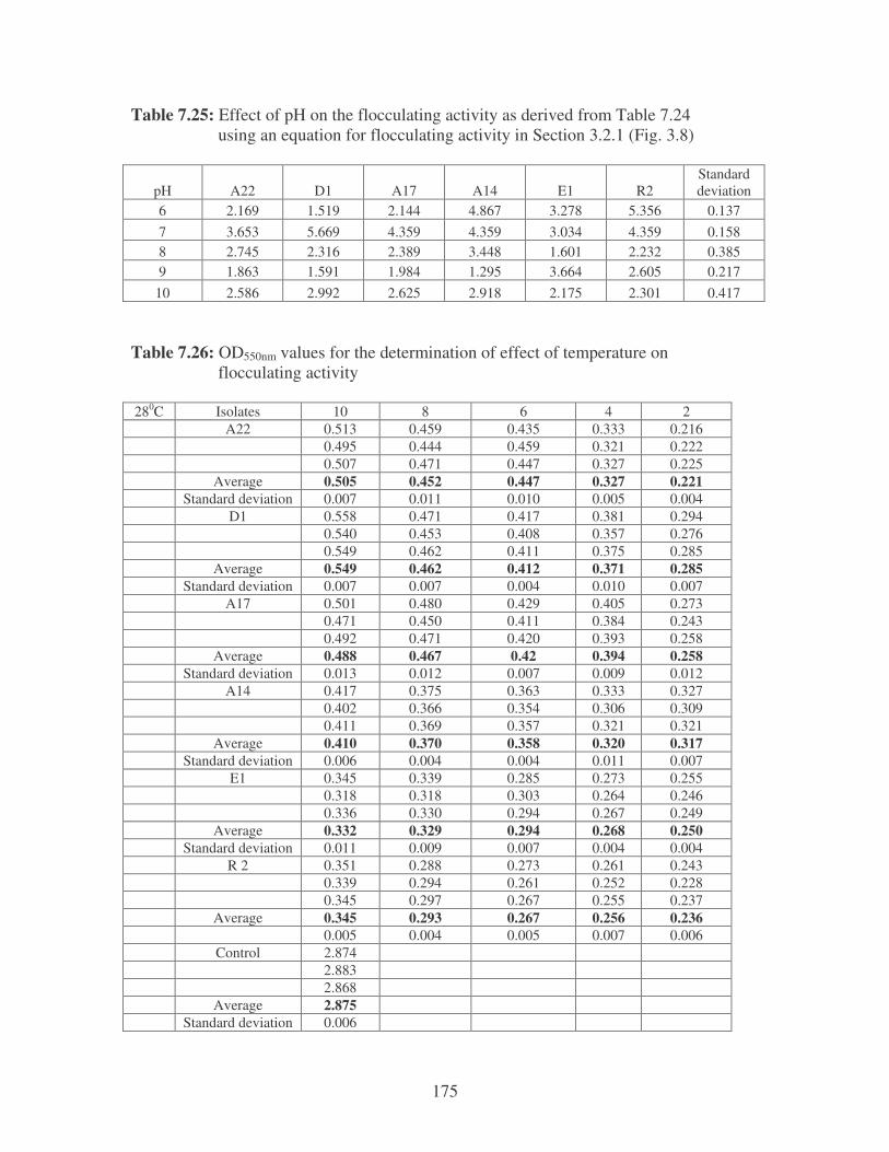
175
Table 7.25: Effect of pH on the flocculating activity as derived from Table 7.24 using an equation for flocculating activity in Section 3.2.1 (Fig. 3.8)
pH A22 D1 A17 A14 E1 R2 Standard deviation
6 2.169 1.519 2.144 4.867 3.278 5.356 0.137 7 3.653 5.669 4.359 4.359 3.034 4.359 0.158 8 2.745 2.316 2.389 3.448 1.601 2.232 0.385 9 1.863 1.591 1.984 1.295 3.664 2.605 0.217
10 2.586 2.992 2.625 2.918 2.175 2.301 0.417 Table 7.26: OD550nm values for the determination of effect of temperature on flocculating activity 280C Isolates 10 8 6 4 2
A22 0.513 0.459 0.435 0.333 0.216 0.495 0.444 0.459 0.321 0.222 0.507 0.471 0.447 0.327 0.225 Average 0.505 0.452 0.447 0.327 0.221 Standard deviation 0.007 0.011 0.010 0.005 0.004 D1 0.558 0.471 0.417 0.381 0.294 0.540 0.453 0.408 0.357 0.276 0.549 0.462 0.411 0.375 0.285 Average 0.549 0.462 0.412 0.371 0.285 Standard deviation 0.007 0.007 0.004 0.010 0.007 A17 0.501 0.480 0.429 0.405 0.273 0.471 0.450 0.411 0.384 0.243 0.492 0.471 0.420 0.393 0.258 Average 0.488 0.467 0.42 0.394 0.258 Standard deviation 0.013 0.012 0.007 0.009 0.012 A14 0.417 0.375 0.363 0.333 0.327 0.402 0.366 0.354 0.306 0.309 0.411 0.369 0.357 0.321 0.321 Average 0.410 0.370 0.358 0.320 0.317 Standard deviation 0.006 0.004 0.004 0.011 0.007 E1 0.345 0.339 0.285 0.273 0.255 0.318 0.318 0.303 0.264 0.246 0.336 0.330 0.294 0.267 0.249 Average 0.332 0.329 0.294 0.268 0.250 Standard deviation 0.011 0.009 0.007 0.004 0.004 R 2 0.351 0.288 0.273 0.261 0.243 0.339 0.294 0.261 0.252 0.228 0.345 0.297 0.267 0.255 0.237 Average 0.345 0.293 0.267 0.256 0.236 0.005 0.004 0.005 0.007 0.006 Control 2.874 2.883 2.868 Average 2.875 Standard deviation 0.006
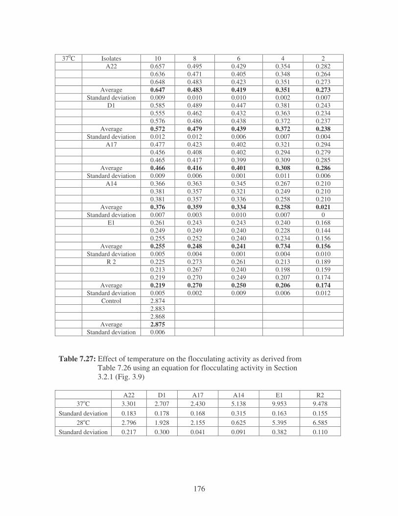
176
370C Isolates 10 8 6 4 2
A22 0.657 0.495 0.429 0.354 0.282 0.636 0.471 0.405 0.348 0.264 0.648 0.483 0.423 0.351 0.273 Average 0.647 0.483 0.419 0.351 0.273 Standard deviation 0.009 0.010 0.010 0.002 0.007 D1 0.585 0.489 0.447 0.381 0.243 0.555 0.462 0.432 0.363 0.234 0.576 0.486 0.438 0.372 0.237 Average 0.572 0.479 0.439 0.372 0.238 Standard deviation 0.012 0.012 0.006 0.007 0.004 A17 0.477 0.423 0.402 0.321 0.294 0.456 0.408 0.402 0.294 0.279 0.465 0.417 0.399 0.309 0.285 Average 0.466 0.416 0.401 0.308 0.286 Standard deviation 0.009 0.006 0.001 0.011 0.006 A14 0.366 0.363 0.345 0.267 0.210 0.381 0.357 0.321 0.249 0.210 0.381 0.357 0.336 0.258 0.210 Average 0.376 0.359 0.334 0.258 0.021 Standard deviation 0.007 0.003 0.010 0.007 0 E1 0.261 0.243 0.243 0.240 0.168 0.249 0.249 0.240 0.228 0.144 0.255 0.252 0.240 0.234 0.156 Average 0.255 0.248 0.241 0.734 0.156 Standard deviation 0.005 0.004 0.001 0.004 0.010 R 2 0.225 0.273 0.261 0.213 0.189 0.213 0.267 0.240 0.198 0.159 0.219 0.270 0.249 0.207 0.174 Average 0.219 0.270 0.250 0.206 0.174 Standard deviation 0.005 0.002 0.009 0.006 0.012 Control 2.874 2.883 2.868 Average 2.875 Standard deviation 0.006
Table 7.27: Effect of temperature on the flocculating activity as derived from Table 7.26 using an equation for flocculating activity in Section 3.2.1 (Fig. 3.9)
A22 D1 A17 A14 E1 R2 37oC 3.301 2.707 2.430 5.138 9.953 9.478
Standard deviation 0.183 0.178 0.168 0.315 0.163 0.155 28oC 2.796 1.928 2.155 0.625 5.395 6.585
Standard deviation 0.217 0.300 0.041 0.091 0.382 0.110
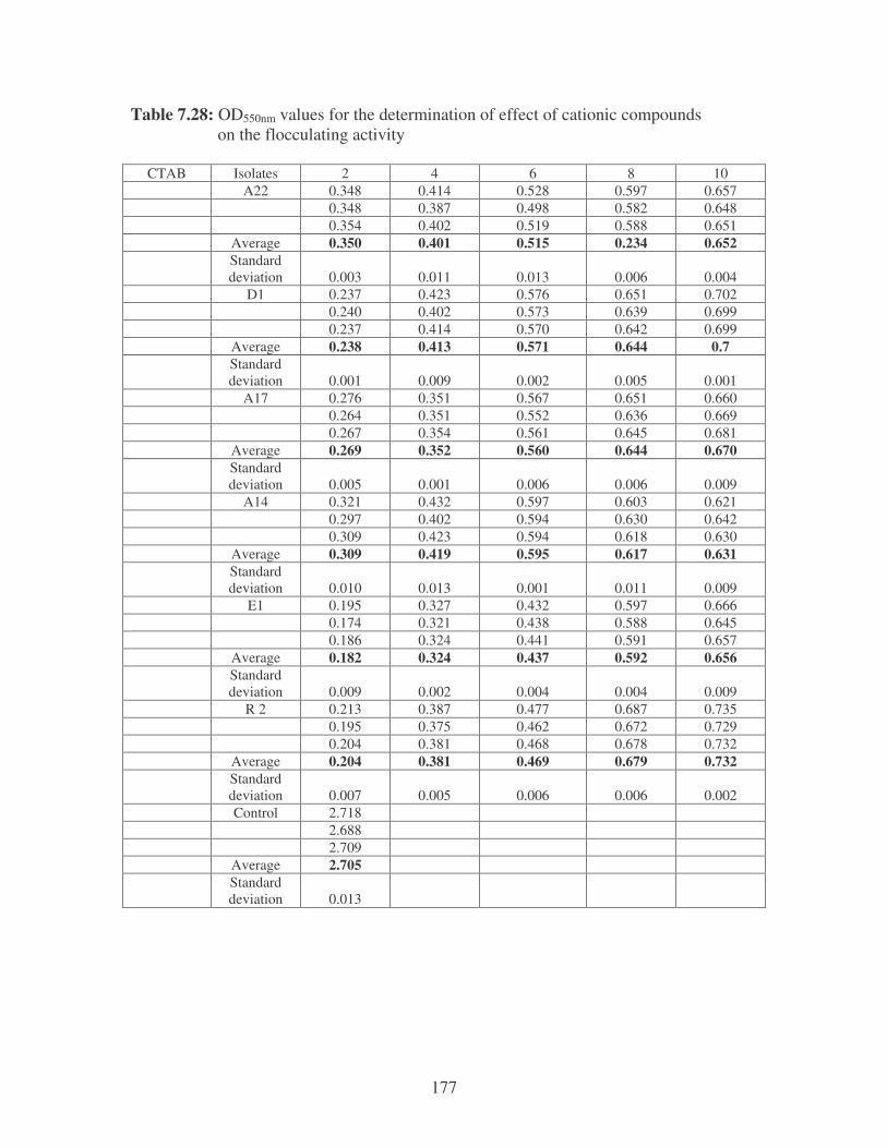
177
Table 7.28: OD550nm values for the determination of effect of cationic compounds on the flocculating activity
CTAB Isolates 2 4 6 8 10 A22 0.348 0.414 0.528 0.597 0.657 0.348 0.387 0.498 0.582 0.648 0.354 0.402 0.519 0.588 0.651 Average 0.350 0.401 0.515 0.234 0.652 Standard
deviation 0.003 0.011 0.013 0.006 0.004 D1 0.237 0.423 0.576 0.651 0.702 0.240 0.402 0.573 0.639 0.699 0.237 0.414 0.570 0.642 0.699 Average 0.238 0.413 0.571 0.644 0.7 Standard
deviation 0.001 0.009 0.002 0.005 0.001 A17 0.276 0.351 0.567 0.651 0.660 0.264 0.351 0.552 0.636 0.669 0.267 0.354 0.561 0.645 0.681 Average 0.269 0.352 0.560 0.644 0.670 Standard
deviation 0.005 0.001 0.006 0.006 0.009 A14 0.321 0.432 0.597 0.603 0.621 0.297 0.402 0.594 0.630 0.642 0.309 0.423 0.594 0.618 0.630 Average 0.309 0.419 0.595 0.617 0.631 Standard
deviation 0.010 0.013 0.001 0.011 0.009 E1 0.195 0.327 0.432 0.597 0.666 0.174 0.321 0.438 0.588 0.645 0.186 0.324 0.441 0.591 0.657 Average 0.182 0.324 0.437 0.592 0.656 Standard
deviation 0.009 0.002 0.004 0.004 0.009 R 2 0.213 0.387 0.477 0.687 0.735 0.195 0.375 0.462 0.672 0.729 0.204 0.381 0.468 0.678 0.732 Average 0.204 0.381 0.469 0.679 0.732 Standard
deviation 0.007 0.005 0.006 0.006 0.002 Control 2.718 2.688 2.709 Average 2.705 Standard
deviation 0.013

178
MgSO4 Isolates 2 4 6 8 10 A22 0.246 0.393 0.477 0.564 0.675 0.216 0.381 0.468 0.546 0.669 0.231 0.387 0.471 0.555 0.672 Average 0.231 0.387 0.471 0.555 0.672 Standard
deviation 0.013 0.005 0.004 0.007 0.002 D1 0.258 0.426 0.519 0.624 0.687 0.240 0.423 0.495 0.606 0.678 0.249 0.432 0.507 0.615 0.681 Average 0.248 0.432 0.507 0.615 0.682 Standard
deviation 0.007 0.004 0.010 0.007 0.004 A17 0.378 0.465 0.471 0.531 0.624 0.351 0.435 0.450 0.516 0.615 0.366 0.456 0.459 0.522 0.618 Average 0.365 0.452 0.46 0.523 0.619 Standard
deviation 0.011 0.013 0.009 0.006 0.004 A14 0.252 0.396 0.465 0.537 0.645 0.264 0.363 0.456 0.519 0.624 0.258 0.381 0.459 0.528 0.633 Average 0.258 0.380 0.460 0.528 0.634 Standard
deviation 0.005 0.014 0.004 0.007 0.009 E1 0.363 0.447 0.591 0.597 0.633 0.384 0.411 0.585 0.588 0.618 0.372 0.426 0.588 0.591 0.624 Average 0.373 0.431 0.588 0.592 0.625 Standard
deviation 0.009 0.015 0.004 0.004 0.006 R 2 0.315 0.477 0.516 0.693 0.708 0.291 0.462 0.528 0.675 0.669 0.303 0.468 0.528 0.684 0.699 Average 0.303 0.469 0.524 0.684 0.692 Standard
deviation 0.010 0.006 0.006 0.007 0.017 Control 2.742 2.733 2.751 Average 2.742 Standard
deviation 0.007
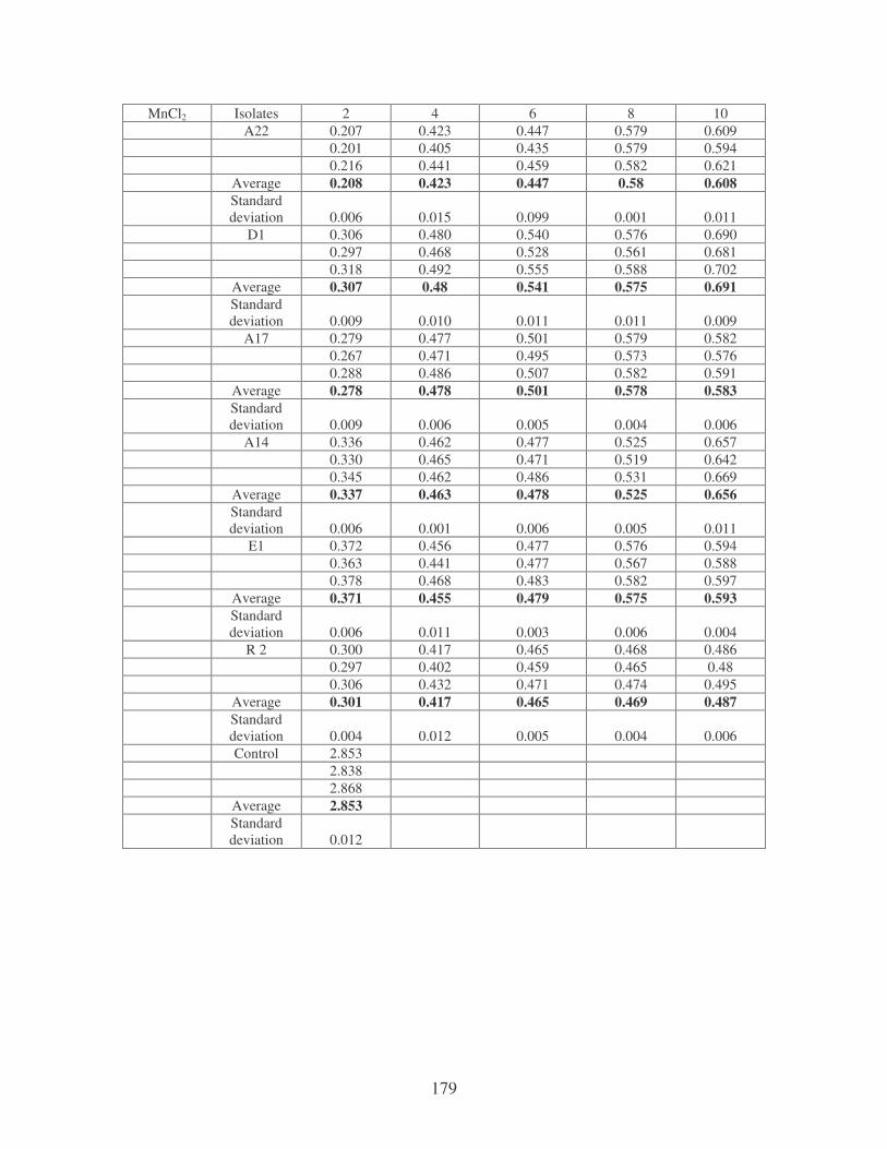
179
MnCl2 Isolates 2 4 6 8 10 A22 0.207 0.423 0.447 0.579 0.609 0.201 0.405 0.435 0.579 0.594 0.216 0.441 0.459 0.582 0.621 Average 0.208 0.423 0.447 0.58 0.608 Standard
deviation 0.006 0.015 0.099 0.001 0.011 D1 0.306 0.480 0.540 0.576 0.690 0.297 0.468 0.528 0.561 0.681 0.318 0.492 0.555 0.588 0.702 Average 0.307 0.48 0.541 0.575 0.691 Standard
deviation 0.009 0.010 0.011 0.011 0.009 A17 0.279 0.477 0.501 0.579 0.582 0.267 0.471 0.495 0.573 0.576 0.288 0.486 0.507 0.582 0.591 Average 0.278 0.478 0.501 0.578 0.583 Standard
deviation 0.009 0.006 0.005 0.004 0.006 A14 0.336 0.462 0.477 0.525 0.657 0.330 0.465 0.471 0.519 0.642 0.345 0.462 0.486 0.531 0.669 Average 0.337 0.463 0.478 0.525 0.656 Standard
deviation 0.006 0.001 0.006 0.005 0.011 E1 0.372 0.456 0.477 0.576 0.594 0.363 0.441 0.477 0.567 0.588 0.378 0.468 0.483 0.582 0.597 Average 0.371 0.455 0.479 0.575 0.593 Standard
deviation 0.006 0.011 0.003 0.006 0.004 R 2 0.300 0.417 0.465 0.468 0.486 0.297 0.402 0.459 0.465 0.48 0.306 0.432 0.471 0.474 0.495 Average 0.301 0.417 0.465 0.469 0.487 Standard
deviation 0.004 0.012 0.005 0.004 0.006 Control 2.853 2.838 2.868 Average 2.853 Standard
deviation 0.012
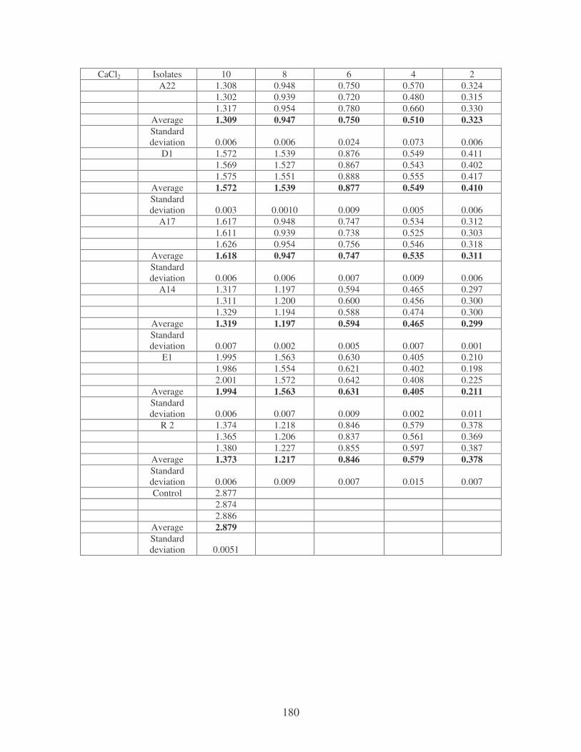
180
CaCl2 Isolates 10 8 6 4 2 A22 1.308 0.948 0.750 0.570 0.324 1.302 0.939 0.720 0.480 0.315 1.317 0.954 0.780 0.660 0.330 Average 1.309 0.947 0.750 0.510 0.323 Standard
deviation 0.006 0.006 0.024 0.073 0.006 D1 1.572 1.539 0.876 0.549 0.411 1.569 1.527 0.867 0.543 0.402 1.575 1.551 0.888 0.555 0.417 Average 1.572 1.539 0.877 0.549 0.410 Standard
deviation 0.003 0.0010 0.009 0.005 0.006 A17 1.617 0.948 0.747 0.534 0.312 1.611 0.939 0.738 0.525 0.303 1.626 0.954 0.756 0.546 0.318 Average 1.618 0.947 0.747 0.535 0.311 Standard
deviation 0.006 0.006 0.007 0.009 0.006 A14 1.317 1.197 0.594 0.465 0.297 1.311 1.200 0.600 0.456 0.300 1.329 1.194 0.588 0.474 0.300 Average 1.319 1.197 0.594 0.465 0.299 Standard
deviation 0.007 0.002 0.005 0.007 0.001 E1 1.995 1.563 0.630 0.405 0.210 1.986 1.554 0.621 0.402 0.198 2.001 1.572 0.642 0.408 0.225 Average 1.994 1.563 0.631 0.405 0.211 Standard
deviation 0.006 0.007 0.009 0.002 0.011 R 2 1.374 1.218 0.846 0.579 0.378 1.365 1.206 0.837 0.561 0.369 1.380 1.227 0.855 0.597 0.387 Average 1.373 1.217 0.846 0.579 0.378 Standard
deviation 0.006 0.009 0.007 0.015 0.007 Control 2.877 2.874 2.886 Average 2.879 Standard
deviation 0.0051
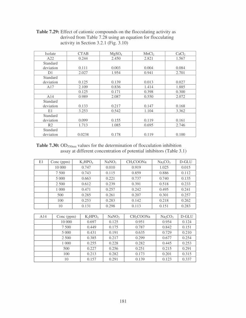
181
Table 7.29: Effect of cationic compounds on the flocculating activity as derived from Table 7.28 using an equation for flocculating activity in Section 3.2.1 (Fig. 3.10)
Isolate CTAB MgSO4 MnCl2 CaCl2 A22 0.244 2.450 2.821 1.567
Standard deviation 0.111 0.003 0.004 0.084
D1 2.027 1.954 0.941 2.701 Standard deviation 0.125 0.139 0.013 0.027
A17 2.109 0.836 1.414 1.885 0.125 0.171 0.398 0.300
A14 0.989 2.087 0.550 2.072 Standard deviation 0.133 0.217 0.147 0.168
E1 3.253 0.542 1.104 3.362 Standard deviation 0.099 0.155 0.119 0.161
R2 1.713 1.085 0.695 2.746 Standard deviation 0.0238 0.178 0.119 0.100
Table 7.30: OD550nm values for the determination of flocculation inhibition assay at different concentration of potential inhibitors (Table 3.1)
E1 Conc (ppm) K2HPO4 NaNO3 CH2COONa Na2CO3 D-GLU 10 000 0.747 0.010 0.919 1.025 0.015 7 500 0.743 0.115 0.859 0.886 0.112 5 000 0.663 0.221 0.737 0.740 0.135 2 500 0.612 0.239 0.391 0.518 0.233 1 000 0.471 0.257 0.242 0.495 0.241 500 0.285 0.261 0.207 0.301 0.257 100 0.253 0.283 0.142 0.218 0.262 10 0.131 0.298 0.113 0.151 0.283
A14 Conc (ppm) K2HPO4 NaNO3 CH2COONa Na2CO3 D-GLU
10 000 0.697 0.125 0.951 0.954 0.124 7 500 0.449 0.175 0.787 0.842 0.151 5 000 0.431 0.191 0.635 0.729 0.210 2 500 0.385 0.217 0.299 0.677 0.254 1 000 0.255 0.228 0.282 0.445 0.253 500 0.227 0.256 0.251 0.215 0.291 100 0.213 0.282 0.173 0.201 0.315 10 0.157 0.291 0.139 0.123 0.337
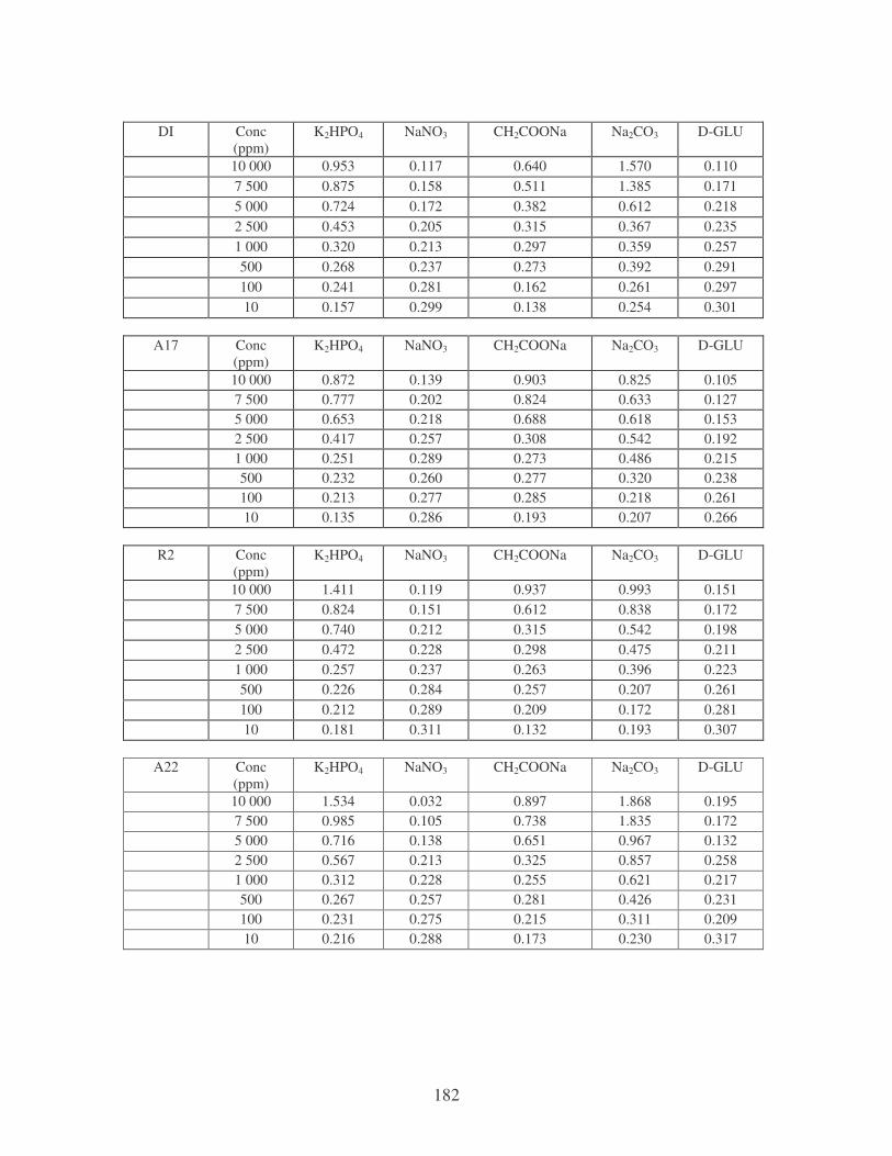
182
DI Conc
(ppm) K2HPO4 NaNO3 CH2COONa Na2CO3 D-GLU
10 000 0.953 0.117 0.640 1.570 0.110 7 500 0.875 0.158 0.511 1.385 0.171 5 000 0.724 0.172 0.382 0.612 0.218 2 500 0.453 0.205 0.315 0.367 0.235 1 000 0.320 0.213 0.297 0.359 0.257 500 0.268 0.237 0.273 0.392 0.291 100 0.241 0.281 0.162 0.261 0.297 10 0.157 0.299 0.138 0.254 0.301
A17 Conc
(ppm) K2HPO4 NaNO3 CH2COONa Na2CO3 D-GLU
10 000 0.872 0.139 0.903 0.825 0.105 7 500 0.777 0.202 0.824 0.633 0.127 5 000 0.653 0.218 0.688 0.618 0.153 2 500 0.417 0.257 0.308 0.542 0.192 1 000 0.251 0.289 0.273 0.486 0.215 500 0.232 0.260 0.277 0.320 0.238 100 0.213 0.277 0.285 0.218 0.261 10 0.135 0.286 0.193 0.207 0.266
R2 Conc
(ppm) K2HPO4 NaNO3 CH2COONa Na2CO3 D-GLU
10 000 1.411 0.119 0.937 0.993 0.151 7 500 0.824 0.151 0.612 0.838 0.172 5 000 0.740 0.212 0.315 0.542 0.198 2 500 0.472 0.228 0.298 0.475 0.211 1 000 0.257 0.237 0.263 0.396 0.223 500 0.226 0.284 0.257 0.207 0.261 100 0.212 0.289 0.209 0.172 0.281 10 0.181 0.311 0.132 0.193 0.307
A22 Conc
(ppm) K2HPO4 NaNO3 CH2COONa Na2CO3 D-GLU
10 000 1.534 0.032 0.897 1.868 0.195 7 500 0.985 0.105 0.738 1.835 0.172 5 000 0.716 0.138 0.651 0.967 0.132 2 500 0.567 0.213 0.325 0.857 0.258 1 000 0.312 0.228 0.255 0.621 0.217 500 0.267 0.257 0.281 0.426 0.231 100 0.231 0.275 0.215 0.311 0.209 10 0.216 0.288 0.173 0.230 0.317
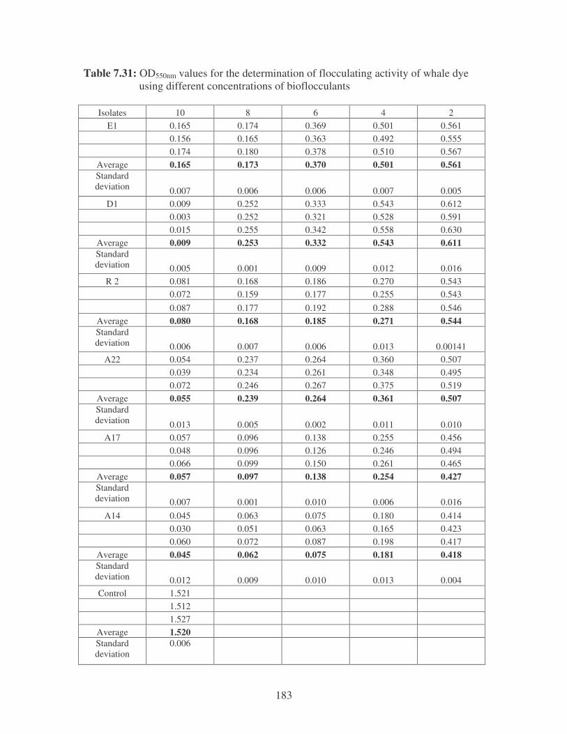
183
Table 7.31: OD550nm values for the determination of flocculating activity of whale dye using different concentrations of bioflocculants
Isolates 10 8 6 4 2 E1 0.165 0.174 0.369 0.501 0.561
0.156 0.165 0.363 0.492 0.555 0.174 0.180 0.378 0.510 0.567
Average 0.165 0.173 0.370 0.501 0.561 Standard deviation 0.007 0.006 0.006 0.007 0.005
D1 0.009 0.252 0.333 0.543 0.612 0.003 0.252 0.321 0.528 0.591 0.015 0.255 0.342 0.558 0.630
Average 0.009 0.253 0.332 0.543 0.611 Standard deviation 0.005 0.001 0.009 0.012 0.016
R 2 0.081 0.168 0.186 0.270 0.543 0.072 0.159 0.177 0.255 0.543 0.087 0.177 0.192 0.288 0.546
Average 0.080 0.168 0.185 0.271 0.544 Standard deviation 0.006 0.007 0.006 0.013 0.00141
A22 0.054 0.237 0.264 0.360 0.507 0.039 0.234 0.261 0.348 0.495 0.072 0.246 0.267 0.375 0.519
Average 0.055 0.239 0.264 0.361 0.507 Standard deviation 0.013 0.005 0.002 0.011 0.010
A17 0.057 0.096 0.138 0.255 0.456 0.048 0.096 0.126 0.246 0.494 0.066 0.099 0.150 0.261 0.465
Average 0.057 0.097 0.138 0.254 0.427 Standard deviation 0.007 0.001 0.010 0.006 0.016
A14 0.045 0.063 0.075 0.180 0.414 0.030 0.051 0.063 0.165 0.423 0.060 0.072 0.087 0.198 0.417
Average 0.045 0.062 0.075 0.181 0.418 Standard deviation 0.012 0.009 0.010 0.013 0.004 Control 1.521
1.512 1.527
Average 1.520 Standard deviation
0.006
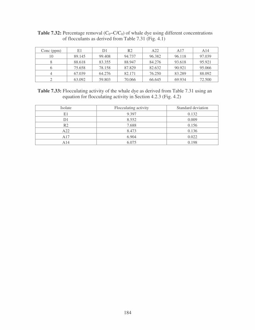
184
Table 7.32: Percentage removal (C0−C/C0) of whale dye using different concentrations of flocculants as derived from Table 7.31 (Fig. 4.1)
Conc (ppm) E1 D1 R2 A22 A17 A14 10 89.145 99.408 94.737 96.382 96.118 97.039 8 88.618 83.355 88.947 84.276 93.618 95.921 6 75.658 78.158 87.829 82.632 90.921 95.066 4 67.039 64.276 82.171 76.250 83.289 88.092 2 63.092 59.803 70.066 66.645 69.934 72.500
Table 7.33: Flocculating activity of the whale dye as derived from Table 7.31 using an equation for flocculating activity in Section 4.2.3 (Fig. 4.2)
Isolate Flocculating activity Standard deviation E1 9.397 0.132 D1 8.552 0.009 R2 7.688 0.156
A22 8.473 0.136 A17 6.904 0.022 A14 6.075 0.198
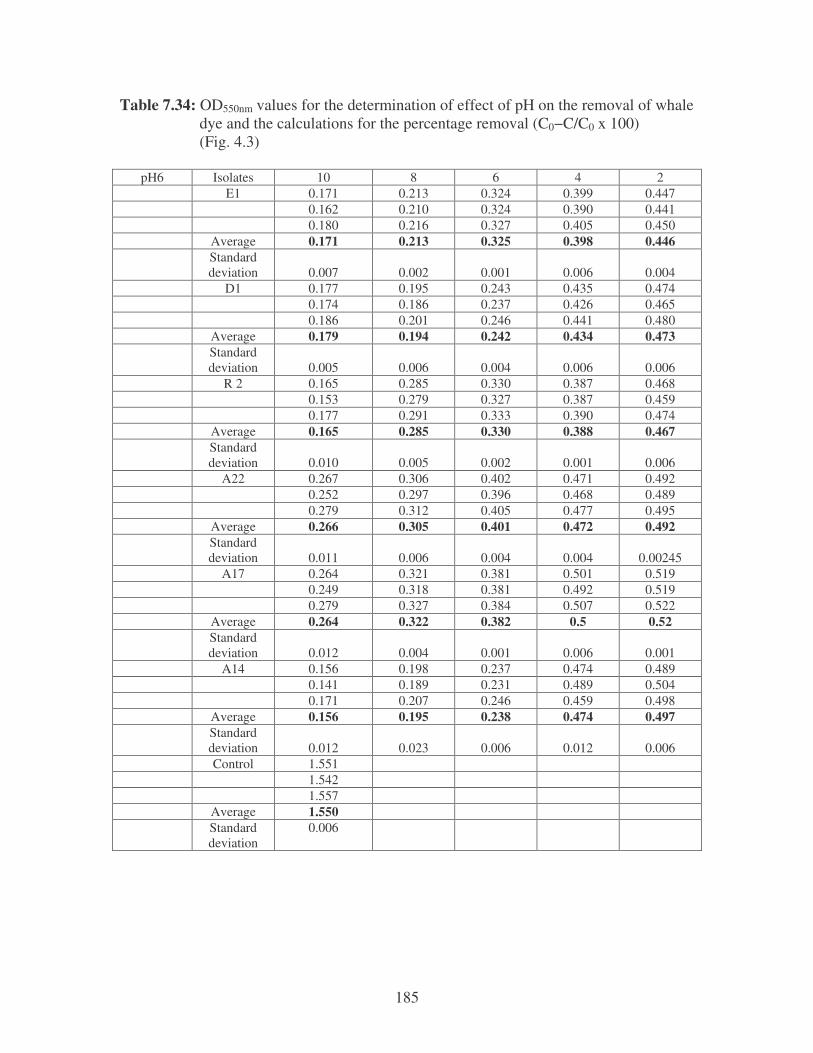
185
Table 7.34: OD550nm values for the determination of effect of pH on the removal of whale dye and the calculations for the percentage removal (C0−C/C0 x 100) (Fig. 4.3)
pH6 Isolates 10 8 6 4 2 E1 0.171 0.213 0.324 0.399 0.447 0.162 0.210 0.324 0.390 0.441 0.180 0.216 0.327 0.405 0.450 Average 0.171 0.213 0.325 0.398 0.446 Standard
deviation 0.007 0.002 0.001 0.006 0.004 D1 0.177 0.195 0.243 0.435 0.474 0.174 0.186 0.237 0.426 0.465 0.186 0.201 0.246 0.441 0.480 Average 0.179 0.194 0.242 0.434 0.473 Standard
deviation 0.005 0.006 0.004 0.006 0.006 R 2 0.165 0.285 0.330 0.387 0.468 0.153 0.279 0.327 0.387 0.459 0.177 0.291 0.333 0.390 0.474 Average 0.165 0.285 0.330 0.388 0.467 Standard
deviation 0.010 0.005 0.002 0.001 0.006 A22 0.267 0.306 0.402 0.471 0.492 0.252 0.297 0.396 0.468 0.489 0.279 0.312 0.405 0.477 0.495 Average 0.266 0.305 0.401 0.472 0.492 Standard
deviation 0.011 0.006 0.004 0.004 0.00245 A17 0.264 0.321 0.381 0.501 0.519 0.249 0.318 0.381 0.492 0.519 0.279 0.327 0.384 0.507 0.522 Average 0.264 0.322 0.382 0.5 0.52 Standard
deviation 0.012 0.004 0.001 0.006 0.001 A14 0.156 0.198 0.237 0.474 0.489 0.141 0.189 0.231 0.489 0.504 0.171 0.207 0.246 0.459 0.498 Average 0.156 0.195 0.238 0.474 0.497 Standard
deviation 0.012 0.023 0.006 0.012 0.006 Control 1.551 1.542 1.557 Average 1.550 Standard
deviation 0.006
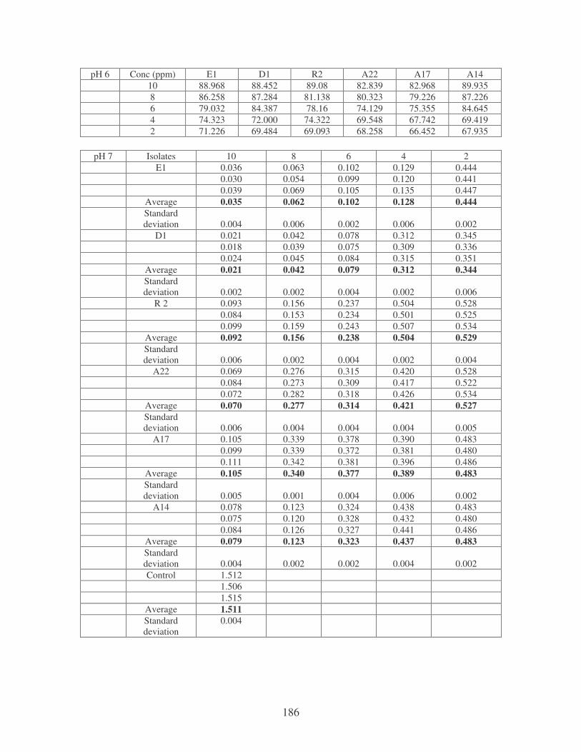
186
pH 6 Conc (ppm) E1 D1 R2 A22 A17 A14 10 88.968 88.452 89.08 82.839 82.968 89.935 8 86.258 87.284 81.138 80.323 79.226 87.226 6 79.032 84.387 78.16 74.129 75.355 84.645 4 74.323 72.000 74.322 69.548 67.742 69.419 2 71.226 69.484 69.093 68.258 66.452 67.935
pH 7 Isolates 10 8 6 4 2
E1 0.036 0.063 0.102 0.129 0.444 0.030 0.054 0.099 0.120 0.441 0.039 0.069 0.105 0.135 0.447 Average 0.035 0.062 0.102 0.128 0.444 Standard
deviation 0.004 0.006 0.002 0.006 0.002 D1 0.021 0.042 0.078 0.312 0.345 0.018 0.039 0.075 0.309 0.336 0.024 0.045 0.084 0.315 0.351 Average 0.021 0.042 0.079 0.312 0.344 Standard
deviation 0.002 0.002 0.004 0.002 0.006 R 2 0.093 0.156 0.237 0.504 0.528 0.084 0.153 0.234 0.501 0.525 0.099 0.159 0.243 0.507 0.534 Average 0.092 0.156 0.238 0.504 0.529 Standard
deviation 0.006 0.002 0.004 0.002 0.004 A22 0.069 0.276 0.315 0.420 0.528 0.084 0.273 0.309 0.417 0.522 0.072 0.282 0.318 0.426 0.534 Average 0.070 0.277 0.314 0.421 0.527 Standard
deviation 0.006 0.004 0.004 0.004 0.005 A17 0.105 0.339 0.378 0.390 0.483 0.099 0.339 0.372 0.381 0.480 0.111 0.342 0.381 0.396 0.486 Average 0.105 0.340 0.377 0.389 0.483 Standard
deviation 0.005 0.001 0.004 0.006 0.002 A14 0.078 0.123 0.324 0.438 0.483 0.075 0.120 0.328 0.432 0.480 0.084 0.126 0.327 0.441 0.486 Average 0.079 0.123 0.323 0.437 0.483 Standard
deviation 0.004 0.002 0.002 0.004 0.002 Control 1.512 1.506 1.515 Average 1.511 Standard
deviation 0.004
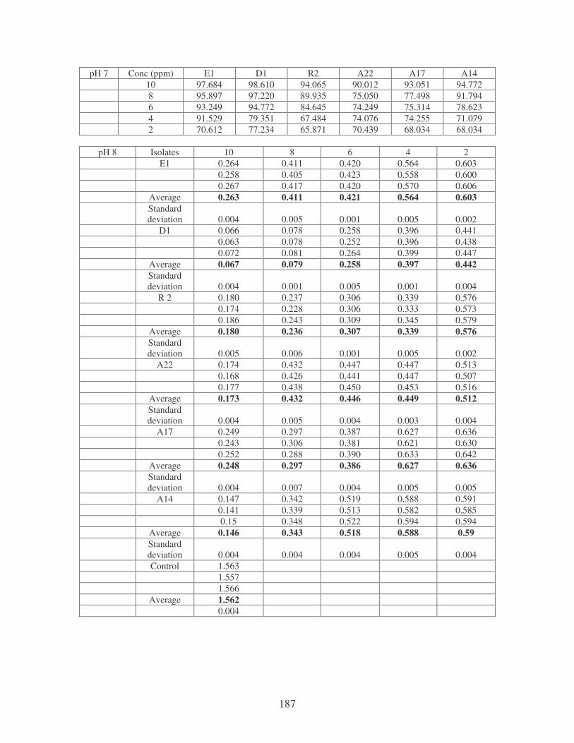
187
pH 7 Conc (ppm) E1 D1 R2 A22 A17 A14 10 97.684 98.610 94.065 90.012 93.051 94.772 8 95.897 97.220 89.935 75.050 77.498 91.794 6 93.249 94.772 84.645 74.249 75.314 78.623 4 91.529 79.351 67.484 74.076 74.255 71.079 2 70.612 77.234 65.871 70.439 68.034 68.034
pH 8 Isolates 10 8 6 4 2
E1 0.264 0.411 0.420 0.564 0.603 0.258 0.405 0.423 0.558 0.600 0.267 0.417 0.420 0.570 0.606 Average 0.263 0.411 0.421 0.564 0.603 Standard
deviation 0.004 0.005 0.001 0.005 0.002 D1 0.066 0.078 0.258 0.396 0.441 0.063 0.078 0.252 0.396 0.438 0.072 0.081 0.264 0.399 0.447 Average 0.067 0.079 0.258 0.397 0.442 Standard
deviation 0.004 0.001 0.005 0.001 0.004 R 2 0.180 0.237 0.306 0.339 0.576 0.174 0.228 0.306 0.333 0.573 0.186 0.243 0.309 0.345 0.579 Average 0.180 0.236 0.307 0.339 0.576 Standard
deviation 0.005 0.006 0.001 0.005 0.002 A22 0.174 0.432 0.447 0.447 0.513 0.168 0.426 0.441 0.447 0.507 0.177 0.438 0.450 0.453 0.516 Average 0.173 0.432 0.446 0.449 0.512 Standard
deviation 0.004 0.005 0.004 0.003 0.004 A17 0.249 0.297 0.387 0.627 0.636 0.243 0.306 0.381 0.621 0.630 0.252 0.288 0.390 0.633 0.642 Average 0.248 0.297 0.386 0.627 0.636 Standard
deviation 0.004 0.007 0.004 0.005 0.005 A14 0.147 0.342 0.519 0.588 0.591 0.141 0.339 0.513 0.582 0.585 0.15 0.348 0.522 0.594 0.594 Average 0.146 0.343 0.518 0.588 0.59 Standard
deviation 0.004 0.004 0.004 0.005 0.004 Control 1.563 1.557 1.566 Average 1.562 0.004
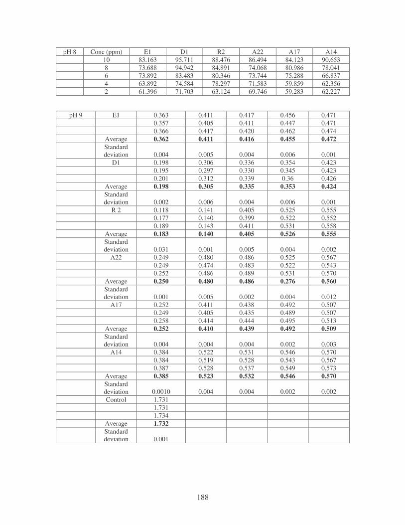
188
pH 8 Conc (ppm) E1 D1 R2 A22 A17 A14 10 83.163 95.711 88.476 86.494 84.123 90.653 8 73.688 94.942 84.891 74.068 80.986 78.041 6 73.892 83.483 80.346 73.744 75.288 66.837 4 63.892 74.584 78.297 71.583 59.859 62.356 2 61.396 71.703 63.124 69.746 59.283 62.227
pH 9 E1 0.363 0.411 0.417 0.456 0.471 0.357 0.405 0.411 0.447 0.471 0.366 0.417 0.420 0.462 0.474 Average 0.362 0.411 0.416 0.455 0.472 Standard
deviation 0.004 0.005 0.004 0.006 0.001 D1 0.198 0.306 0.336 0.354 0.423 0.195 0.297 0.330 0.345 0.423 0.201 0.312 0.339 0.36 0.426 Average 0.198 0.305 0.335 0.353 0.424 Standard
deviation 0.002 0.006 0.004 0.006 0.001 R 2 0.118 0.141 0.405 0.525 0.555 0.177 0.140 0.399 0.522 0.552 0.189 0.143 0.411 0.531 0.558 Average 0.183 0.140 0.405 0.526 0.555 Standard
deviation 0.031 0.001 0.005 0.004 0.002 A22 0.249 0.480 0.486 0.525 0.567 0.249 0.474 0.483 0.522 0.543 0.252 0.486 0.489 0.531 0.570 Average 0.250 0.480 0.486 0.276 0.560 Standard
deviation 0.001 0.005 0.002 0.004 0.012 A17 0.252 0.411 0.438 0.492 0.507 0.249 0.405 0.435 0.489 0.507 0.258 0.414 0.444 0.495 0.513 Average 0.252 0.410 0.439 0.492 0.509 Standard
deviation 0.004 0.004 0.004 0.002 0.003 A14 0.384 0.522 0.531 0.546 0.570 0.384 0.519 0.528 0.543 0.567 0.387 0.528 0.537 0.549 0.573 Average 0.385 0.523 0.532 0.546 0.570 Standard
deviation 0.0010 0.004 0.004 0.002 0.002 Control 1.731 1.731 1.734 Average 1.732 Standard
deviation 0.001
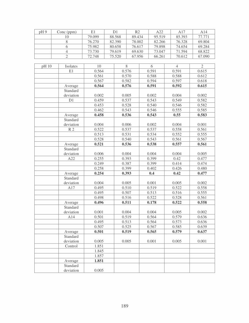
189
pH 9 Conc (ppm) E1 D1 R2 A22 A17 A14 10 79.099 88.568 89.434 95.519 85.393 77.771 8 76.270 82.390 78.002 82.266 76.328 69.804 6 75.982 80.658 76.617 79.898 74.654 69.284 4 73.730 79.619 69.630 73.047 71.594 68.822 2 72.748 75.520 67.956 66.261 70.612 67.090
pH 10 Isolates 10 8 6 4 2
E1 0.564 0.576 0.591 0.591 0.615 0.561 0.570 0.588 0.588 0.612 0.567 0.582 0.594 0.597 0.618 Average 0.564 0.576 0.591 0.592 0.615 Standard
deviation 0.002 0.005 0.002 0.004 0.002 D1 0.459 0.537 0.543 0.549 0.582 0.453 0.528 0.540 0.546 0.582 0.462 0.543 0.546 0.555 0.585 Average 0.458 0.536 0.543 0.55 0.583 Standard
deviation 0.004 0.006 0.002 0.004 0.001 R 2 0.522 0.537 0.537 0.558 0.561 0.513 0.531 0.534 0.552 0.555 0.528 0.540 0.543 0.561 0.567 Average 0.521 0.536 0.538 0.557 0.561 Standard
deviation 0.006 0.004 0.004 0.004 0.005 A22 0.255 0.393 0.399 0.42 0.477 0.249 0.387 0.399 0.414 0.474 0.258 0.399 0.402 0.426 0.480 Average 0.254 0.393 0.4 0.42 0.477 Standard
deviation 0.004 0.005 0.001 0.005 0.002 A17 0.495 0.510 0.519 0.522 0.558 0.495 0.507 0.513 0.516 0.555 0.498 0.516 0.522 0.528 0.561 Average 0.496 0.511 0.178 0.522 0.558 Standard
deviation 0.001 0.004 0.004 0.005 0.002 A14 0.501 0.519 0.564 0.579 0.636 0.495 0.513 0.564 0.573 0.636 0.507 0.525 0.567 0.585 0.639 Average 0.501 0.519 0.565 0.579 0.637 Standard
deviation 0.005 0.005 0.001 0.005 0.001 Control 1.851 1.845 1.857 Average 1.851 Standard
deviation 0.005
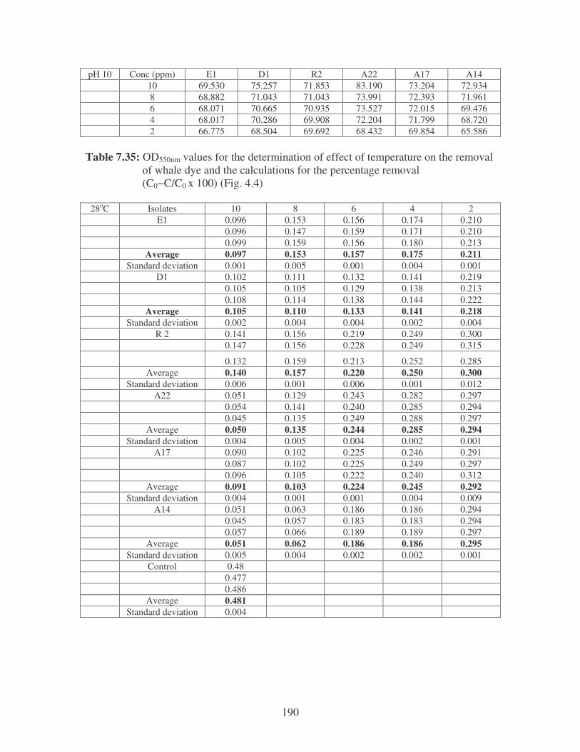
190
pH 10 Conc (ppm) E1 D1 R2 A22 A17 A14 10 69.530 75.257 71.853 83.190 73.204 72.934 8 68.882 71.043 71.043 73.991 72.393 71.961 6 68.071 70.665 70.935 73.527 72.015 69.476 4 68.017 70.286 69.908 72.204 71.799 68.720 2 66.775 68.504 69.692 68.432 69.854 65.586
Table 7.35: OD550nm values for the determination of effect of temperature on the removal of whale dye and the calculations for the percentage removal (C0−C/C0 x 100) (Fig. 4.4)
28oC Isolates 10 8 6 4 2 E1 0.096 0.153 0.156 0.174 0.210 0.096 0.147 0.159 0.171 0.210 0.099 0.159 0.156 0.180 0.213 Average 0.097 0.153 0.157 0.175 0.211 Standard deviation 0.001 0.005 0.001 0.004 0.001 D1 0.102 0.111 0.132 0.141 0.219 0.105 0.105 0.129 0.138 0.213 0.108 0.114 0.138 0.144 0.222 Average 0.105 0.110 0.133 0.141 0.218 Standard deviation 0.002 0.004 0.004 0.002 0.004 R 2 0.141 0.156 0.219 0.249 0.300 0.147 0.156 0.228 0.249 0.315 0.132 0.159 0.213 0.252 0.285 Average 0.140 0.157 0.220 0.250 0.300 Standard deviation 0.006 0.001 0.006 0.001 0.012 A22 0.051 0.129 0.243 0.282 0.297 0.054 0.141 0.240 0.285 0.294 0.045 0.135 0.249 0.288 0.297 Average 0.050 0.135 0.244 0.285 0.294 Standard deviation 0.004 0.005 0.004 0.002 0.001 A17 0.090 0.102 0.225 0.246 0.291 0.087 0.102 0.225 0.249 0.297 0.096 0.105 0.222 0.240 0.312 Average 0.091 0.103 0.224 0.245 0.292 Standard deviation 0.004 0.001 0.001 0.004 0.009 A14 0.051 0.063 0.186 0.186 0.294 0.045 0.057 0.183 0.183 0.294 0.057 0.066 0.189 0.189 0.297 Average 0.051 0.062 0.186 0.186 0.295 Standard deviation 0.005 0.004 0.002 0.002 0.001 Control 0.48 0.477 0.486 Average 0.481 Standard deviation 0.004

191
28oC Conc (ppm) E1 D1 R2 A22 A17 A14 10 79.834 78.170 76.299 88.009 81.081 87.770 8 68.191 77.131 67.360 67.626 78.586 85.132 6 67.360 72.249 54.262 41.487 53.430 67.386 4 63.617 70.686 46.362 31.655 49.064 55.396 2 56.133 54.678 37.630 29.496 39.293 29.257
35oC Isolates 10 8 6 4 2 E1 0.009 0.033 0.117 0.123 0.174 0.006 0.024 0.111 0.117 0.168 0.015 0.039 0.120 0.129 0.180 Average 0.010 0.032 0.116 0.122 0.174 Standard
deviation 0.004 0.006 0.004 0.005 0.005 D1 0.006 0.201 0.207 0.228 0.255 0.003 0.201 0.204 0.228 0.246 0.006 0.204 0.213 0.231 0.261 Average 0.005 0.202 0.208 0.229 0.254 Standard
deviation 0.001 0.001 0.004 0.001 0.006 R 2 0.006 0.042 0.057 0.087 0.132 0.006 0.039 0.057 0.087 0.129 0.006 0.048 0.060 0.093 0.135 Average 0.006 0.043 0.058 0.089 0.132 Standard
deviation 0 0.004 0.001 0.003 0.005 A22 0.012 0.066 0.108 0.114 0.117 0.006 0.075 0.105 0.114 0.108 0.015 0.063 0.114 0.117 0.123 Average 0.011 0.068 0.109 0.115 0.116 Standard
deviation 0.004 0.005 0.004 0.001 0.006 A17 0.021 0.087 0.129 0.162 0.216 0.015 0.081 0.123 0.153 0.210 0.027 0.090 0.132 0.168 0.219 Average 0.021 0.086 0.128 0.161 0.215 Standard
deviation 0.005 0.004 0.004 0.006 0.004 A14 0.009 0.042 0.072 0.114 0.117 0.012 0.039 0.069 0.105 0.111 0.006 0.048 0.075 0.12 0.123 Average 0.009 0.043 0.072 0.113 0.117 Standard
deviation 0.002 0.004 0.002 0.006 0.004 Control 0.417 0.414 0.402 Average 0.417 Standard
deviation 0.006
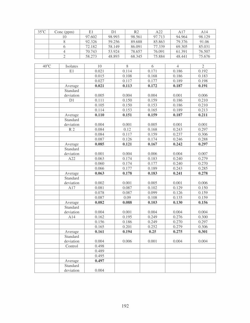
192
35oC Conc (ppm) E1 D1 R2 A22 A17 A14 10 97.602 98.993 98.561 97.713 94.964 98.129 8 92.326 59.256 89.688 85.863 79.376 91.06 6 72.182 58.149 86.091 77.339 69.305 85.031 4 70.743 53.924 78.657 76.091 61.391 76.507 2 58.273 48.893 68.345 75.884 48.441 75.676
40oC Isolates 10 8 6 4 2
E1 0.021 0.114 0.171 0.186 0.192 0.015 0.108 0.168 0.186 0.183 0.027 0.117 0.177 0.189 0.198 Average 0.021 0.113 0.172 0.187 0.191 Standard
deviation 0.005 0.004 0.004 0.001 0.006 D1 0.111 0.150 0.159 0.186 0.210 0.105 0.150 0.153 0.186 0.210 0.114 0.153 0.165 0.189 0.213 Average 0.110 0.151 0.159 0.187 0.211 Standard
deviation 0.004 0.001 0.005 0.001 0.001 R 2 0.084 0.12 0.168 0.243 0.297 0.084 0.117 0.159 0.237 0.306 0.087 0.126 0.174 0.246 0.288 Average 0.085 0.121 0.167 0.242 0.297 Standard
deviation 0.001 0.004 0.006 0.004 0.007 A22 0.063 0.174 0.183 0.240 0.279 0.060 0.174 0.177 0.240 0.270 0.066 0.177 0.189 0.243 0.285 Average 0.063 0.178 0.183 0.241 0.278 Standard
deviation 0.002 0.001 0.005 0.001 0.006 A17 0.081 0.087 0.102 0.129 0.150 0.078 0.087 0.099 0.126 0.159 0.087 0.09 0.108 0.135 0.159 Average 0.082 0.088 0.103 0.130 0.156 Standard
deviation 0.004 0.001 0.004 0.004 0.004 A14 0.162 0.195 0.249 0.276 0.300 0.156 0.186 0.249 0.270 0.297 0.165 0.201 0.252 0.279 0.306 Average 0.161 0.194 0.25 0.275 0.301 Standard
deviation 0.004 0.006 0.001 0.004 0.004 Control 0.498 0.489 0.495 Average 0.497 Standard
deviation 0.004
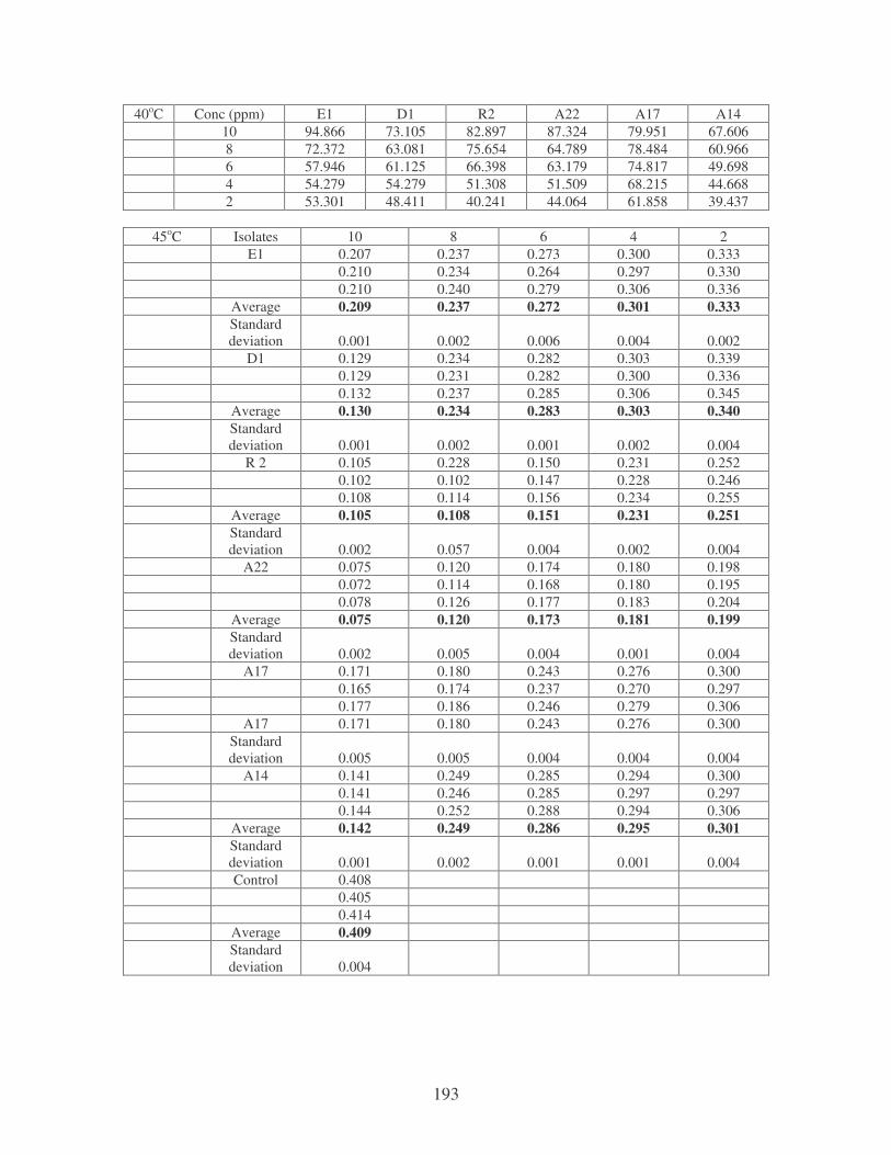
193
40oC Conc (ppm) E1 D1 R2 A22 A17 A14 10 94.866 73.105 82.897 87.324 79.951 67.606 8 72.372 63.081 75.654 64.789 78.484 60.966 6 57.946 61.125 66.398 63.179 74.817 49.698 4 54.279 54.279 51.308 51.509 68.215 44.668 2 53.301 48.411 40.241 44.064 61.858 39.437
45oC Isolates 10 8 6 4 2
E1 0.207 0.237 0.273 0.300 0.333 0.210 0.234 0.264 0.297 0.330 0.210 0.240 0.279 0.306 0.336 Average 0.209 0.237 0.272 0.301 0.333 Standard
deviation 0.001 0.002 0.006 0.004 0.002 D1 0.129 0.234 0.282 0.303 0.339 0.129 0.231 0.282 0.300 0.336 0.132 0.237 0.285 0.306 0.345 Average 0.130 0.234 0.283 0.303 0.340 Standard
deviation 0.001 0.002 0.001 0.002 0.004 R 2 0.105 0.228 0.150 0.231 0.252 0.102 0.102 0.147 0.228 0.246 0.108 0.114 0.156 0.234 0.255 Average 0.105 0.108 0.151 0.231 0.251 Standard
deviation 0.002 0.057 0.004 0.002 0.004 A22 0.075 0.120 0.174 0.180 0.198 0.072 0.114 0.168 0.180 0.195 0.078 0.126 0.177 0.183 0.204 Average 0.075 0.120 0.173 0.181 0.199 Standard
deviation 0.002 0.005 0.004 0.001 0.004 A17 0.171 0.180 0.243 0.276 0.300 0.165 0.174 0.237 0.270 0.297 0.177 0.186 0.246 0.279 0.306 A17 0.171 0.180 0.243 0.276 0.300 Standard
deviation 0.005 0.005 0.004 0.004 0.004 A14 0.141 0.249 0.285 0.294 0.300 0.141 0.246 0.285 0.297 0.297 0.144 0.252 0.288 0.294 0.306 Average 0.142 0.249 0.286 0.295 0.301 Standard
deviation 0.001 0.002 0.001 0.001 0.004 Control 0.408 0.405 0.414 Average 0.409 Standard
deviation 0.004
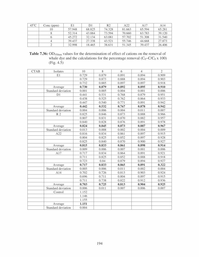
194
45oC Conc (ppm) E1 D1 R2 A22 A17 A14 10 57.948 68.825 74.328 81.663 65.594 65.281 8 52.314 43.884 73.594 70.660 63.783 39.120 6 45.272 32.134 63.081 57.702 51.308 31.540 4 39.437 27.338 43.521 55.746 44.668 27.873 2 32.998 18.465 38.631 51.345 39.437 26.406
Table 7.36: OD550nm values for the determination of effect of cations on the removal of whale dye and the calculations for the percentage removal (C0−C/C0 x 100) (Fig. 4.5)
CTAB Isolates 10 8 6 4 2 E1 0.729 0.879 0.891 0.894 0.909 0.729 0.873 0.888 0.894 0.903 0.732 0.885 0.897 0.897 0.918 Average 0.730 0.879 0.892 0.895 0.910 Standard deviation 0.001 0.005 0.004 0.001 0.006 D1 0.441 0.531 0.768 0.879 0.951 0.438 0.525 0.762 0.864 0.933 0.447 0.540 0.771 0.891 0.942 Average 0.442 0.532 0.767 0.878 0.942 Standard deviation 0.004 0.006 0.004 0.011 0.007 R 2 0.825 0.846 0.873 0.888 0.966 0.807 0.831 0.870 0.882 0.957 0.840 0.828 0.876 0.891 0.978 Average 0.824 0.845 0.873 0.887 0.967 Standard deviation 0.013 0.008 0.002 0.004 0.009 A22 0.816 0.834 0.861 0.897 0.915 0.804 0.825 0.852 0.897 0.928 0.825 0.840 0.870 0.900 0.927 Average 0.815 0.833 0.861 0.898 0.914 Standard deviation 0.009 0.006 0.007 0.001 0.006 A17 0.717 0.834 0.864 0.891 0.921 0.711 0.825 0.852 0.888 0.918 0.723 0.84 0.879 0.894 0.927 Average 0.717 0.833 0.865 0.891 0.322 Standard deviation 0.005 0.006 0.011 0.002 0.004 A14 0.702 0.726 0.813 0.903 0.924 0.696 0.711 0.804 0.897 0.915 0.711 0.738 0.822 0.912 0.936 Average 0.703 0.725 0.813 0.904 0.925 Standard deviation 0.006 0.011 0.007 0.006 0.007 Control 1.152 1.146 1.155 Average 1.151 Standard deviation 0.004

195
CTAB Conc (ppm) E1 D1 R2 A22 A17 A14 10 36.577 61.599 28.410 29.192 37.706 38.923 8 23.632 53.779 26.586 27.628 27.628 37.011 6 22.502 33.362 24.153 25.195 24.848 29.366 4 22.242 23.719 22.937 21.981 22.589 21.460 2 20.938 18.158 15.986 20.591 19.896 19.635
CaCl2 Isolates 10 8 6 4 2
E1 0.087 0.087 0.09 0.09 0.144 0.075 0.078 0.087 0.099 0.135 0.099 0.102 0.096 0.096 0.15 Average 0.087 0.089 0.091 0.097 0.143 Standard
deviation 0.008 0.010 0.004 0.004 0.006 D1 0.066 0.084 0.087 0.099 0.102 0.048 0.078 0.072 0.09 0.096 0.081 0.090 0.102 0.108 0.108 Average 0.065 0.084 0.087 0.099 0.102 Standard
deviation 0.013 0.005 0.012 0.007 0.005 R 2 0.072 0.096 0.111 0.123 0.147 0.060 0.084 0.105 0.108 0.138 0.084 0.108 0.117 0.135 0.156 Average 0.072 0.096 0.111 0.122 0.147 Standard
deviation 0.010 0.010 0.005 0.011 0.007 A22 0.063 0.072 0.084 0.084 0.114 0.057 0.063 0.078 0.078 0.108 0.066 0.078 0.087 0.093 0.123 Average 0.062 0.071 0.083 0.085 0.115 Standard
deviation 0.004 0.006 0.004 0.006 0.006 A17 0.069 0.078 0.084 0.09 0.135 0.066 0.069 0.066 0.078 0.132 0.072 0.087 0.102 0.102 0.141 Average 0.069 0.078 0.084 0.09 0.136 Standard
deviation 0.002 0.007 0.015 0.010 0.004 A14 0.069 0.072 0.078 0.087 0.090 0.060 0.066 0.069 0.069 0.075 0.081 0.081 0.084 0.105 0.105 Average 0.070 0.073 0.077 0.087 0.090 Standard
deviation 0.009 0.006 0.006 0.015 0.012 Control 0.276 0.267 0.282 Average 0.275 Standard
deviation 0.006

196
CaCl2 Conc (ppm) E1 D1 R2 A22 A17 A14 10 68.364 75.364 73.818 77.455 74.909 74.545 8 67.636 69.455 65.091 74.182 71.636 73.455 6 66.909 68.364 60.000 69.818 69.455 72.000 4 64.727 64.000 55.636 69.091 67.273 68.364 2 48.000 62.909 46.546 58.182 50.545 67.273
MnCl2 Isolates 10 8 6 4 2
E1 0.003 0.006 0.009 0.012 0.015 0 0.009 0.012 0.006 0.009 0 0.006 0.006 0.015 0.018 Average 0.001 0.007 0.009 0.011 0.014 Standard
deviation 0.001 0.001 0.002 0.004 0.004 D1 0.003 0.009 0.012 0.018 0.024 0.003 0.012 0.006 0.009 0.009 0 0.006 0.021 0.027 0.036 Average 0.002 0.009 0.013 0.018 0.023 Standard
deviation 0.001 0.002 0.006 0.007 0.011 R 2 0.003 0.003 0.015 0.018 0.021 0.003 0.006 0.006 0.006 0.018 0 0.003 0.021 0.015 0.027 Average 0.002 0.004 0.014 0.017 0.022 Standard
deviation 0.001 0.001 0.006 0.005 0.004 A22 0.003 0.009 0.015 0.021 0.024 0 0.012 0.006 0.018 0.018 0 0.006 0.024 0.024 0.030 Average 0.001 0.009 0.015 0.021 0.024 Standard
deviation 0.001 0.002 0.007 0.002 0.005 A17 0.003 0.003 0.006 0.009 0.009 0 0.006 0.003 0.012 0.012 0 0.003 0.012 0.006 0.009 Average 0.001 0.004 0.007 0.009 0.010 Standard
deviation 0.005 0.001 0.004 0.002 0.001 A14 0.003 0.009 0.012 0.015 0.009 0.003 0.012 0.006 0.012 0.018 0.003 0.006 0.021 0.021 0.018 Average 0.003 0.009 0.013 0.016 0.018 Standard
deviation 0 0.002 0.006 0.004 0.004 Control 0.111 0.105 0.117 Average 0.111 Standard
deviation 0.005
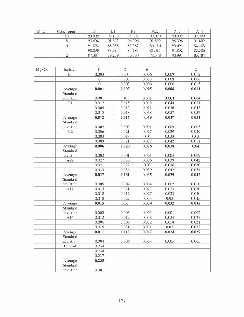
197
MnCl2 Conc (ppm) E1 D1 R2 A22 A17 A14 10 99.099 98.198 98.198 99.099 99.099 97.209 8 93.694 91.892 96.396 91.892 96.396 91.892 6 91.892 88.288 87.387 86.486 93.694 88.288 4 90.090 83.784 84.685 81.081 91.892 85.586 2 87.387 79.279 80.180 78.378 90.991 83.784
MgSO4 Isolates 10 8 6 4 2 E1 0.003 0.003 0.006 0.009 0.012 0 0.003 0.003 0.009 0.006 0 0.003 0.006 0.006 0.015 Average 0.001 0.003 0.005 0.008 0.011 Standard
deviation 0.001 0 0.001 0.001 0.004 D1 0.012 0.015 0.018 0.048 0.051 0.009 0.012 0.021 0.036 0.045 0.015 0.018 0.018 0.057 0.057 Average 0.012 0.015 0.019 0.047 0.051 Standard
deviation 0.002 0.002 0.001 0.009 0.005 R 2 0.006 0.021 0.027 0.039 0.039 0.003 0.018 0.03 0.033 0.03 0.009 0.021 0.027 0.042 0.051 Average 0.006 0.020 0.028 0.038 0.04 Standard
deviation 0.002 0.001 0.001 0.004 0.009 A22 0.027 0.030 0.036 0.039 0.042 0.021 0.027 0.03 0.036 0.030 0.033 0.036 0.039 0.042 0.054 Average 0.027 0.131 0.035 0.039 0.042 Standard
deviation 0.005 0.004 0.004 0.002 0.010 A17 0.015 0.021 0.027 0.033 0.030 0.012 0.012 0.027 0.033 0.030 0.018 0.027 0.033 0.03 0.045 Average 0.015 0.02 0.029 0.032 0.035 Standard
deviation 0.002 0.006 0.003 0.001 0.007 A14 0.012 0.012 0.018 0.024 0.027 0.006 0.006 0.012 0.018 0.021 0.015 0.021 0.021 0.03 0.033 Average 0.011 0.013 0.017 0.024 0.027 Standard
deviation 0.004 0.006 0.004 0.005 0.005 Control 0.234 0.234 0.237 Average 0.235 Standard
deviation 0.001
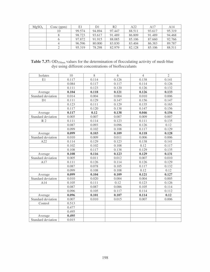
198
MgSO4 Conc (ppm) E1 D1 R2 A22 A17 A14 10 99.574 94.894 97.447 88.511 93.617 95.319 8 98.723 93.617 91.489 86.809 91.489 94.468 6 97.872 91.915 88.085 85.106 87.660 92.766 4 96.596 80.000 83.830 83.404 86.383 89.787 2 95.319 78.298 82.979 82.128 85.106 88.511
Table 7.37: OD550nm values for the determination of flocculating activity of medi-blue dye using different concentrations of bioflocculants
Isolates 10 8 6 4 2 E1 0.117 0.114 0.126 0.138 0.141
0.084 0.117 0.117 0.114 0.126 0.111 0.123 0.120 0.126 0.132
Average 0.104 0.118 0.121 0.126 0.133 Standard deviation 0.014 0.004 0.004 0.010 0.006
D1 0.111 0.129 0.147 0.156 0.147 0.123 0.111 0.129 0.135 0.165 0.117 0.120 0.138 0.147 0.156
Average 0.117 0.12 0.138 0.046 0.156 Standard deviation 0.005 0.007 0.007 0.009 0.007
R 2 0.111 0.114 0.123 0.111 0.135 0.087 0.093 0.096 0.126 0.12 0.099 0.102 0.108 0.117 0.129
Average 0.099 0.103 0.109 0.118 0.128 Standard deviation 0.010 0.009 0.011 0.006 0.006
A22 0.114 0.129 0.123 0.138 0.141 0.102 0.102 0.108 0.12 0.117 0.108 0.117 0.138 0.129 0.135
Average 0.108 0.116 0.123 0.129 0.131 Standard deviation 0.005 0.011 0.012 0.007 0.010
A17 0.111 0.126 0.114 0.126 0.129 0.087 0.078 0.105 0.117 0.132 0.099 0.108 0.108 0.12 0.12
Average 0.099 0.104 0.109 0.121 0.127 Standard deviation 0.010 0.020 0.004 0.004 0.005
A14 0.105 0.111 0.12 0.123 0.126 0.087 0.087 0.086 0.105 0.114 0.096 0.105 0.117 0.114 0.112
Average 0.096 0.101 0.107 0.114 0.12 Standard deviation 0.007 0.010 0.015 0.007 0.006
Control 0.513 0.477 0.495
Average 0.495 Standard deviation 0.015
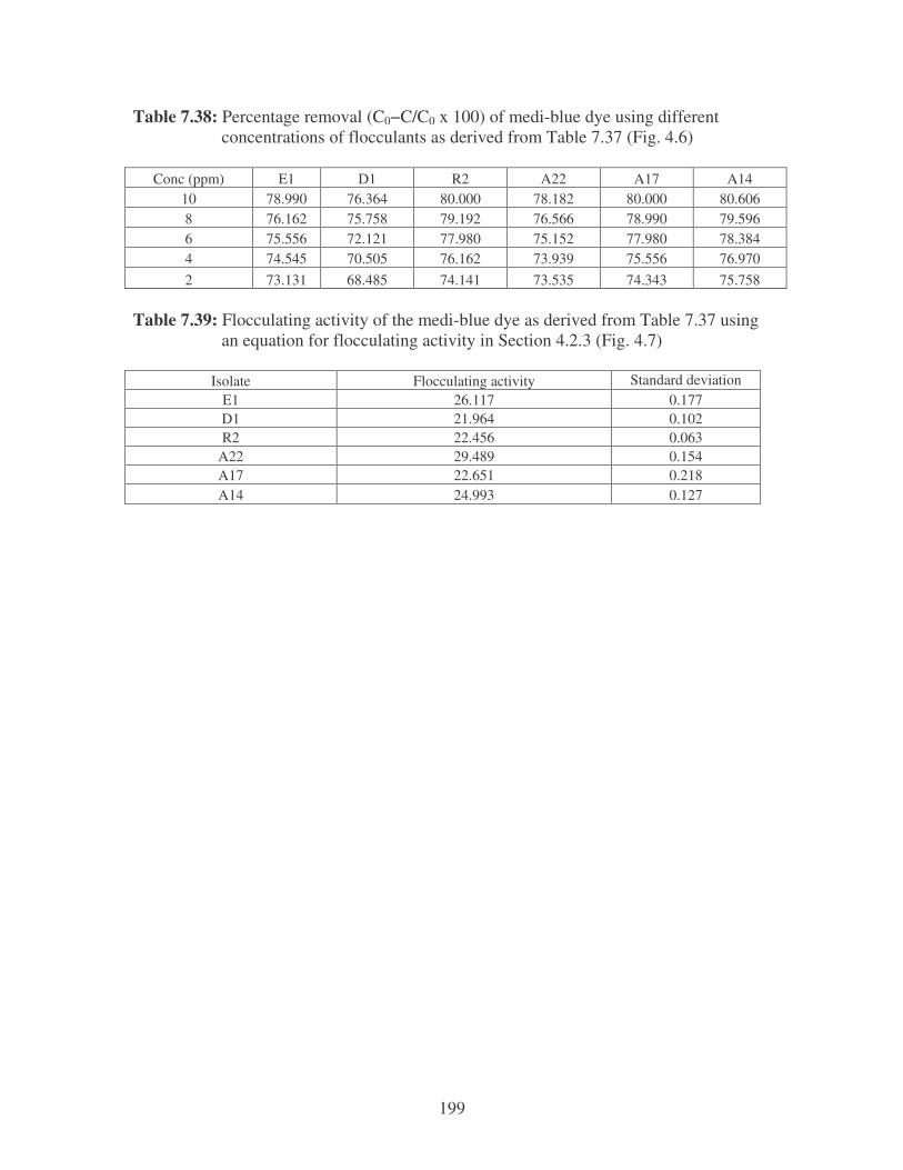
199
Table 7.38: Percentage removal (C0−C/C0 x 100) of medi-blue dye using different concentrations of flocculants as derived from Table 7.37 (Fig. 4.6)
Conc (ppm) E1 D1 R2 A22 A17 A14 10 78.990 76.364 80.000 78.182 80.000 80.606 8 76.162 75.758 79.192 76.566 78.990 79.596 6 75.556 72.121 77.980 75.152 77.980 78.384 4 74.545 70.505 76.162 73.939 75.556 76.970 2 73.131 68.485 74.141 73.535 74.343 75.758
Table 7.39: Flocculating activity of the medi-blue dye as derived from Table 7.37 using an equation for flocculating activity in Section 4.2.3 (Fig. 4.7)
Isolate Flocculating activity Standard deviation E1 26.117 0.177 D1 21.964 0.102 R2 22.456 0.063
A22 29.489 0.154 A17 22.651 0.218 A14 24.993 0.127
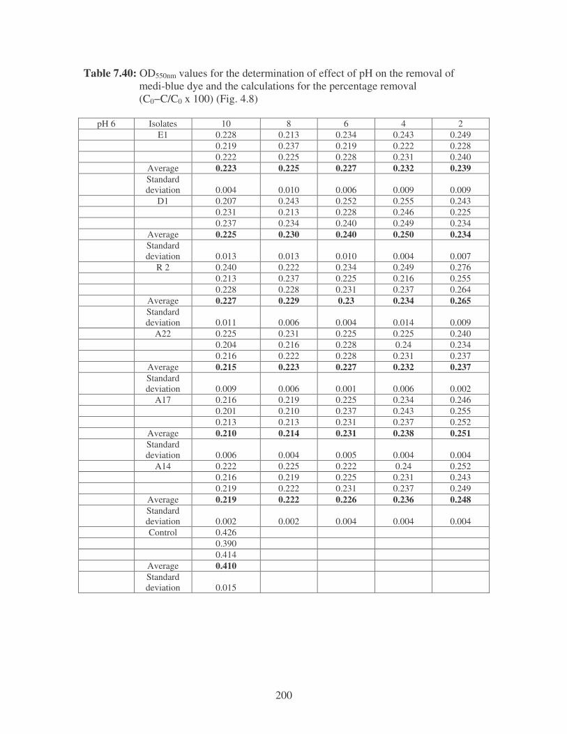
200
Table 7.40: OD550nm values for the determination of effect of pH on the removal of medi-blue dye and the calculations for the percentage removal (C0−C/C0 x 100) (Fig. 4.8)
pH 6 Isolates 10 8 6 4 2 E1 0.228 0.213 0.234 0.243 0.249 0.219 0.237 0.219 0.222 0.228 0.222 0.225 0.228 0.231 0.240 Average 0.223 0.225 0.227 0.232 0.239 Standard
deviation 0.004 0.010 0.006 0.009 0.009 D1 0.207 0.243 0.252 0.255 0.243 0.231 0.213 0.228 0.246 0.225 0.237 0.234 0.240 0.249 0.234 Average 0.225 0.230 0.240 0.250 0.234 Standard
deviation 0.013 0.013 0.010 0.004 0.007 R 2 0.240 0.222 0.234 0.249 0.276 0.213 0.237 0.225 0.216 0.255 0.228 0.228 0.231 0.237 0.264 Average 0.227 0.229 0.23 0.234 0.265 Standard
deviation 0.011 0.006 0.004 0.014 0.009 A22 0.225 0.231 0.225 0.225 0.240 0.204 0.216 0.228 0.24 0.234 0.216 0.222 0.228 0.231 0.237 Average 0.215 0.223 0.227 0.232 0.237 Standard
deviation 0.009 0.006 0.001 0.006 0.002 A17 0.216 0.219 0.225 0.234 0.246 0.201 0.210 0.237 0.243 0.255 0.213 0.213 0.231 0.237 0.252 Average 0.210 0.214 0.231 0.238 0.251 Standard
deviation 0.006 0.004 0.005 0.004 0.004 A14 0.222 0.225 0.222 0.24 0.252 0.216 0.219 0.225 0.231 0.243 0.219 0.222 0.231 0.237 0.249 Average 0.219 0.222 0.226 0.236 0.248 Standard
deviation 0.002 0.002 0.004 0.004 0.004 Control 0.426 0.390 0.414 Average 0.410 Standard
deviation 0.015
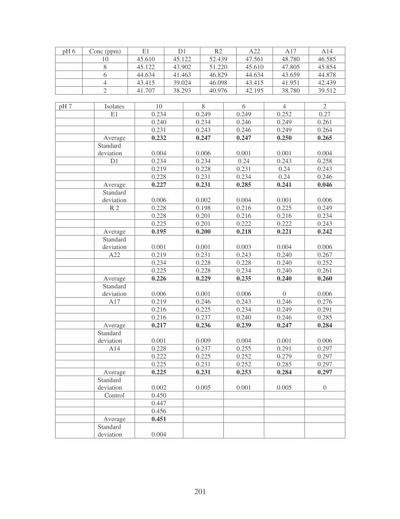
201
pH 6 Conc (ppm) E1 D1 R2 A22 A17 A14 10 45.610 45.122 52.439 47.561 48.780 46.585 8 45.122 43.902 51.220 45.610 47.805 45.854 6 44.634 41.463 46.829 44.634 43.659 44.878 4 43.415 39.024 46.098 43.415 41.951 42.439 2 41.707 38.293 40.976 42.195 38.780 39.512
pH 7 Isolates 10 8 6 4 2 E1 0.234 0.249 0.249 0.252 0.27 0.240 0.234 0.246 0.249 0.261 0.231 0.243 0.246 0.249 0.264 Average 0.232 0.247 0.247 0.250 0.265 Standard
deviation 0.004 0.006 0.001 0.001 0.004 D1 0.234 0.234 0.24 0.243 0.258 0.219 0.228 0.231 0.24 0.243 0.228 0.231 0.234 0.24 0.246 Average 0.227 0.231 0.285 0.241 0.046 Standard
deviation 0.006 0.002 0.004 0.001 0.006 R 2 0.228 0.198 0.216 0.225 0.249 0.228 0.201 0.216 0.216 0.234 0.225 0.201 0.222 0.222 0.243 Average 0.195 0.200 0.218 0.221 0.242 Standard
deviation 0.001 0.001 0.003 0.004 0.006 A22 0.219 0.231 0.243 0.240 0.267 0.234 0.228 0.228 0.240 0.252 0.225 0.228 0.234 0.240 0.261 Average 0.226 0.229 0.235 0.240 0.260 Standard
deviation 0.006 0.001 0.006 0 0.006 A17 0.219 0.246 0.243 0.246 0.276 0.216 0.225 0.234 0.249 0.291 0.216 0.237 0.240 0.246 0.285 Average 0.217 0.236 0.239 0.247 0.284 Standard
deviation 0.001 0.009 0.004 0.001 0.006 A14 0.228 0.237 0.255 0.291 0.297 0.222 0.225 0.252 0.279 0.297 0.225 0.231 0.252 0.285 0.297 Average 0.225 0.231 0.253 0.284 0.297 Standard
deviation 0.002 0.005 0.001 0.005 0 Control 0.450 0.447 0.456 Average 0.451 Standard
deviation 0.004
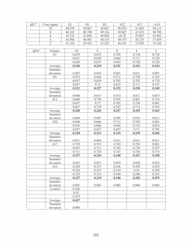
202
pH 7 Conc (ppm) E1 D1 R2 A22 A17 A14 10 48.559 49.667 49.667 50.554 51.885 50.111 8 46.341 48.780 49.224 49.667 47.672 48.780 6 45.233 47.894 49.002 48.78 47.007 43.902 4 44.568 46.563 48.115 48.337 45.233 37.029 2 41.242 45.455 41.242 46.341 37.029 34.146
pH 8 Isolates 10 8 6 4 2
E1 0.639 0.675 0.702 0.738 0.738 0.621 0.630 0.684 0.711 0.720 0.630 0.657 0.693 0.720 0.729 Average 0.210 0.218 0.231 0.241 0.243 Standard
deviation 0.007 0.018 0.007 0.011 0.007 D1 0.675 0.684 0.711 0.729 0.765 0.657 0.639 0.702 0.702 0.729 0.657 0.72 0.675 0.711 0.747 Average 0.221 0.227 0.232 0.238 0.249 Standard
deviation 0.008 0.033 0.015 0.011 0.015 R 2 0.666 0.738 0.765 0.801 0.774 0.657 0.72 0.765 0.756 0.801 0.657 0.729 0.783 0.774 0.792 Average 0.220 0.243 0.257 0.259 0.263 Standard
deviation 0.004 0.007 0.008 0.018 0.011 A22 0.666 0.666 0.711 0.702 0.801 0.639 0.666 0.684 0.729 0.819 0.657 0.657 0.693 0.72 0.792 Average 0.218 0.221 0.232 0.239 0.266 Standard
deviation 0.011 0.004 0.011 0.011 0.011 A17 0.729 0.747 0.720 0.783 0.801 0.693 0.711 0.765 0.720 0.747 0.711 0.729 0.747 0.756 0.774 Average 0.237 0.243 0.248 0.251 0.258 Standard
deviation 0.015 0.015 0.019 0.026 0.022 A14 0.228 0.231 0.246 0.249 0.252 0.228 0.237 0.234 0.24 0.258 0.225 0.234 0.240 0.246 0.255 Average 0.227 0.234 0.240 0.245 0.255 Standard
deviation 0.001 0.002 0.005 0.004 0.002 Control 0.426 0.42 0.435 Average 0.427 Standard
deviation 0.006
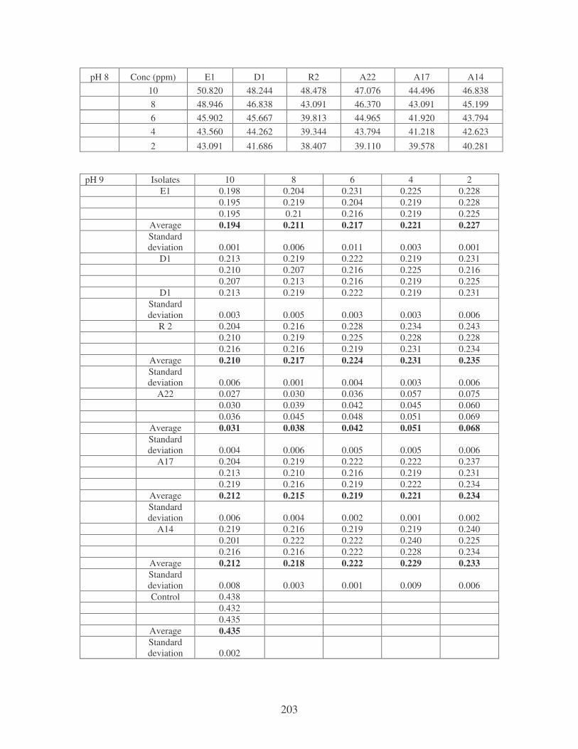
203
pH 8 Conc (ppm) E1 D1 R2 A22 A17 A14 10 50.820 48.244 48.478 47.076 44.496 46.838 8 48.946 46.838 43.091 46.370 43.091 45.199 6 45.902 45.667 39.813 44.965 41.920 43.794 4 43.560 44.262 39.344 43.794 41.218 42.623
2 43.091 41.686 38.407 39.110 39.578 40.281 pH 9 Isolates 10 8 6 4 2 E1 0.198 0.204 0.231 0.225 0.228 0.195 0.219 0.204 0.219 0.228 0.195 0.21 0.216 0.219 0.225 Average 0.194 0.211 0.217 0.221 0.227 Standard
deviation 0.001 0.006 0.011 0.003 0.001 D1 0.213 0.219 0.222 0.219 0.231 0.210 0.207 0.216 0.225 0.216 0.207 0.213 0.216 0.219 0.225 D1 0.213 0.219 0.222 0.219 0.231 Standard
deviation 0.003 0.005 0.003 0.003 0.006 R 2 0.204 0.216 0.228 0.234 0.243 0.210 0.219 0.225 0.228 0.228 0.216 0.216 0.219 0.231 0.234 Average 0.210 0.217 0.224 0.231 0.235 Standard
deviation 0.006 0.001 0.004 0.003 0.006 A22 0.027 0.030 0.036 0.057 0.075 0.030 0.039 0.042 0.045 0.060 0.036 0.045 0.048 0.051 0.069 Average 0.031 0.038 0.042 0.051 0.068 Standard
deviation 0.004 0.006 0.005 0.005 0.006 A17 0.204 0.219 0.222 0.222 0.237 0.213 0.210 0.216 0.219 0.231 0.219 0.216 0.219 0.222 0.234 Average 0.212 0.215 0.219 0.221 0.234 Standard
deviation 0.006 0.004 0.002 0.001 0.002 A14 0.219 0.216 0.219 0.219 0.240 0.201 0.222 0.222 0.240 0.225 0.216 0.216 0.222 0.228 0.234 Average 0.212 0.218 0.222 0.229 0.233 Standard
deviation 0.008 0.003 0.001 0.009 0.006 Control 0.438 0.432 0.435 Average 0.435 Standard
deviation 0.002
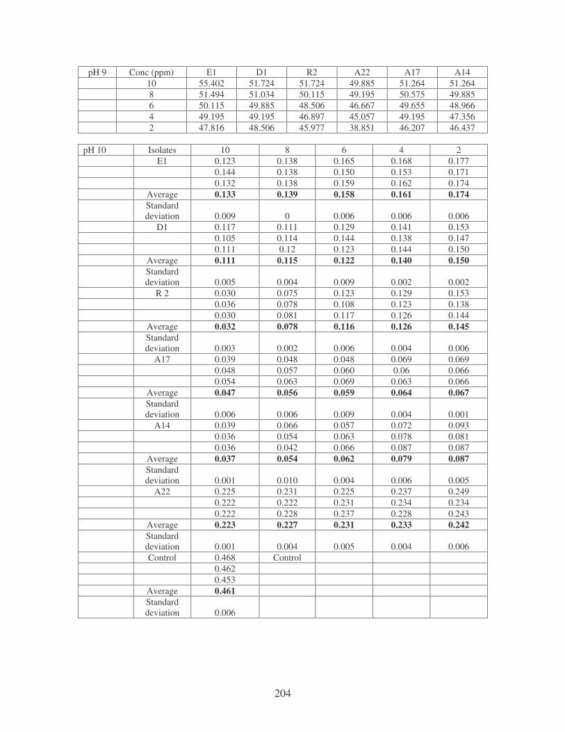
204
pH 9 Conc (ppm) E1 D1 R2 A22 A17 A14 10 55.402 51.724 51.724 49.885 51.264 51.264 8 51.494 51.034 50.115 49.195 50.575 49.885 6 50.115 49.885 48.506 46.667 49.655 48.966 4 49.195 49.195 46.897 45.057 49.195 47.356 2 47.816 48.506 45.977 38.851 46.207 46.437
pH 10 Isolates 10 8 6 4 2 E1 0.123 0.138 0.165 0.168 0.177 0.144 0.138 0.150 0.153 0.171 0.132 0.138 0.159 0.162 0.174 Average 0.133 0.139 0.158 0.161 0.174 Standard
deviation 0.009 0 0.006 0.006 0.006 D1 0.117 0.111 0.129 0.141 0.153 0.105 0.114 0.144 0.138 0.147 0.111 0.12 0.123 0.144 0.150 Average 0.111 0.115 0.122 0.140 0.150 Standard
deviation 0.005 0.004 0.009 0.002 0.002 R 2 0.030 0.075 0.123 0.129 0.153 0.036 0.078 0.108 0.123 0.138 0.030 0.081 0.117 0.126 0.144 Average 0.032 0.078 0.116 0.126 0.145 Standard
deviation 0.003 0.002 0.006 0.004 0.006 A17 0.039 0.048 0.048 0.069 0.069 0.048 0.057 0.060 0.06 0.066 0.054 0.063 0.069 0.063 0.066 Average 0.047 0.056 0.059 0.064 0.067 Standard
deviation 0.006 0.006 0.009 0.004 0.001 A14 0.039 0.066 0.057 0.072 0.093 0.036 0.054 0.063 0.078 0.081 0.036 0.042 0.066 0.087 0.087 Average 0.037 0.054 0.062 0.079 0.087 Standard
deviation 0.001 0.010 0.004 0.006 0.005 A22 0.225 0.231 0.225 0.237 0.249 0.222 0.222 0.231 0.234 0.234 0.222 0.228 0.237 0.228 0.243 Average 0.223 0.227 0.231 0.233 0.242 Standard
deviation 0.001 0.004 0.005 0.004 0.006 Control 0.468 Control 0.462 0.453 Average 0.461 Standard
deviation 0.006
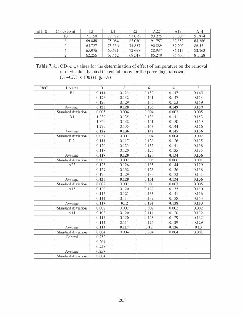
205
pH 10 Conc (ppm) E1 D1 R2 A22 A17 A14 10 71.150 75.922 93.059 93.275 89.805 91.974 8 69.848 75.054 83.080 91.757 87.852 88.286 6 65.727 73.536 74.837 90.889 87.202 86.551 4 65.076 69.631 72.668 88.937 86.117 82.863 2 62.256 67.462 68.547 85.249 85.466 81.128
Table 7.41: OD550nm values for the determination of effect of temperature on the removal of medi-blue dye and the calculations for the percentage removal (C0−C/C0 x 100) (Fig. 4.9)
28oC Isolates 10 8 6 4 2 E1 0.114 0.123 0.132 0.147 0.165 0.126 0.132 0.141 0.147 0.153 0.120 0.129 0.135 0.153 0.159 Average 0.120 0.128 0.136 0.149 0.159 Standard deviation 0.005 0.004 0.004 0.003 0.005 D1 1.230 0.135 0.138 0.141 0.153 1.320 0.138 0.141 0.150 0.159 1.290 0.135 0.147 0.144 0.156 Average 0.128 0.136 0.142 0.145 0.156 Standard deviation 0.037 0.001 0.004 0.004 0.002 R 2 0.114 0.117 0.120 0.126 0.135 0.120 0.123 0.132 0.141 0.138 0.117 0.120 0.126 0.135 0.135 Average 0.117 0.120 0.126 0.134 0.136 Standard deviation 0.002 0.002 0.005 0.006 0.001 A22 0.123 0.126 0.135 0.144 0.129 0.129 0.132 0.123 0.126 0.138 0.126 0.129 0.135 0.132 0.141 Average 0.126 0.128 0.131 0.134 0.136 Standard deviation 0.002 0.002 0.006 0.007 0.005 A17 0.120 0.120 0.129 0.135 0.150 0.117 0.123 0.135 0.141 0.156 0.114 0.117 0.132 0.138 0.153 Average 0.117 0.12 0.132 0.138 0.153 Standard deviation 0.002 0.002 0.002 0.002 0.002 A14 0.108 0.120 0.114 0.120 0.132 0.117 0.120 0.123 0.129 0.132 0.114 0.111 0.123 0.129 0.129 Average 0.113 0.117 0.12 0.126 0.13 Standard deviation 0.004 0.004 0.004 0.004 0.001 Control 0.252 0.261 0.258 Average 0.257 Standard deviation 0.004
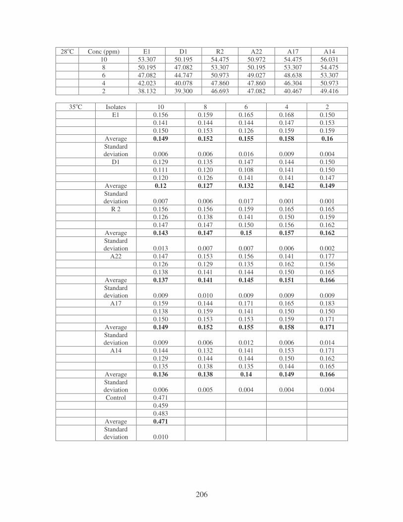
206
28oC Conc (ppm) E1 D1 R2 A22 A17 A14 10 53.307 50.195 54.475 50.972 54.475 56.031 8 50.195 47.082 53.307 50.195 53.307 54.475 6 47.082 44.747 50.973 49.027 48.638 53.307 4 42.023 40.078 47.860 47.860 46.304 50.973 2 38.132 39.300 46.693 47.082 40.467 49.416
35oC Isolates 10 8 6 4 2
E1 0.156 0.159 0.165 0.168 0.150 0.141 0.144 0.144 0.147 0.153 0.150 0.153 0.126 0.159 0.159 Average 0.149 0.152 0.155 0.158 0.16 Standard
deviation 0.006 0.006 0.016 0.009 0.004 D1 0.129 0.135 0.147 0.144 0.150 0.111 0.120 0.108 0.141 0.150 0.120 0.126 0.141 0.141 0.147 Average 0.12 0.127 0.132 0.142 0.149 Standard
deviation 0.007 0.006 0.017 0.001 0.001 R 2 0.156 0.156 0.159 0.165 0.165 0.126 0.138 0.141 0.150 0.159 0.147 0.147 0.150 0.156 0.162 Average 0.143 0.147 0.15 0.157 0.162 Standard
deviation 0.013 0.007 0.007 0.006 0.002 A22 0.147 0.153 0.156 0.141 0.177 0.126 0.129 0.135 0.162 0.156 0.138 0.141 0.144 0.150 0.165 Average 0.137 0.141 0.145 0.151 0.166 Standard
deviation 0.009 0.010 0.009 0.009 0.009 A17 0.159 0.144 0.171 0.165 0.183 0.138 0.159 0.141 0.150 0.150 0.150 0.153 0.153 0.159 0.171 Average 0.149 0.152 0.155 0.158 0.171 Standard
deviation 0.009 0.006 0.012 0.006 0.014 A14 0.144 0.132 0.141 0.153 0.171 0.129 0.144 0.144 0.150 0.162 0.135 0.138 0.135 0.144 0.165 Average 0.136 0.138 0.14 0.149 0.166 Standard
deviation 0.006 0.005 0.004 0.004 0.004 Control 0.471 0.459 0.483 Average 0.471 Standard
deviation 0.010

207
35oC Conc (ppm) E1 D1 R2 A22 A17 A14 10 68.365 74.522 69.639 70.913 68.365 71.125 8 67.728 73.036 68.970 70.064 67.091 70.701 6 67.091 71.975 68.153 69.214 67.091 70.276 4 66.454 69.851 66.667 67.941 66.454 68.365 2 66.030 68.365 65.605 64.756 63.694 64.756
40oC Isolates 10 8 6 4 2
E1 0.165 0.183 0.162 0.195 0.198 0.165 0.153 0.183 0.18 0.189 0.171 0.174 0.174 0.189 0.192 Average 0.167 0.170 0.173 0.188 0.193 Standard
deviation 0.003 0.013 0.009 0.006 0.004 D1 0.180 0.183 0.195 0.195 0.198 0.156 0.162 0.177 0.186 0.198 0.174 0.174 0.186 0.192 0.195 Average 0.170 0.173 0.186 0.191 0.197 Standard
deviation 0.011 0.009 0.007 0.004 0.001 R 2 0.162 0.159 0.183 0.186 0.195 0.138 0.168 0.174 0.183 0.183 0.156 0.162 0.177 0.183 0.189 Average 0.152 0.163 0.178 0.184 0.189 Standard
deviation 0.010 0.004 0.004 0.001 0.005 A22 0.186 0.195 0.198 0.189 0.207 0.165 0.183 0.189 0.201 0.198 0.177 0.189 0.192 0.195 0.189 Average 0.176 0.189 0.193 0.195 0.198 Standard
deviation 0.009 0.005 0.004 0.005 0.007 A17 0.165 0.168 0.174 0.192 0.201 0.156 0.171 0.180 0.177 0.213 0.159 0.168 0.177 0.186 0.207 Average 0.160 0.169 0.177 0.185 0.207 Standard
deviation 0.004 0.001 0.002 0.006 0.005 A14 0.171 0.180 0.219 0.210 0.249 0.186 0.195 0.210 0.225 0.240 0.180 0.189 0.213 0.219 0.243 Average 0.179 0.188 0.21 0.218 0.244 Standard
deviation 0.006 0.006 0.004 0.006 0.004 Control 0.417 0.420 0.417 Average 0.418 Standard
deviation 0.001
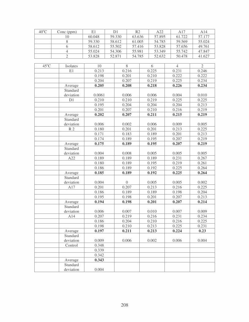
208
40oC Conc (ppm) E1 D1 R2 A22 A17 A14 10 60.048 59.330 63.636 57.895 61.722 57.177 8 59.330 58.612 61.005 54.785 59.569 55.024 6 58.612 55.502 57.416 53.828 57.656 49.761 4 55.024 54.306 55.981 53.349 55.742 47.847 2 53.828 52.871 54.785 52.632 50.478 41.627
45oC Isolates 10 8 6 4 2
E1 0.213 0.216 0.225 0.231 0.246 0.198 0.201 0.210 0.222 0.222 0.204 0.207 0.219 0.225 0.234 Average 0.205 0.208 0.218 0.226 0.234 Standard
deviation 0.0061 0.006 0.006 0.004 0.010 D1 0.210 0.210 0.219 0.225 0.225 0.195 0.204 0.204 0.204 0.213 0.201 0.207 0.210 0.216 0.219 Average 0.202 0.207 0.211 0.215 0.219 Standard
deviation 0.006 0.002 0.006 0.009 0.005 R 2 0.180 0.201 0.201 0.213 0.225 0.171 0.183 0.189 0.201 0.213 0.174 0.189 0.195 0.207 0.219 Average 0.175 0.189 0.195 0.207 0.219 Standard
deviation 0.004 0.008 0.005 0.005 0.005 A22 0.189 0.189 0.189 0.231 0.267 0.180 0.189 0.195 0.219 0.261 0.186 0.189 0.192 0.225 0.264 Average 0.185 0.189 0.192 0.225 0.264 Standard
deviation 0.004 0 0.005 0.005 0.002 A17 0.201 0.207 0.213 0.216 0.225 0.186 0.189 0.189 0.198 0.204 0.195 0.198 0.201 0.207 0.213 Average 0.194 0.198 0.201 0.207 0.214 Standard
deviation 0.006 0.007 0.010 0.007 0.009 A14 0.207 0.219 0.216 0.231 0.234 0.186 0.204 0.210 0.216 0.225 0.198 0.210 0.213 0.225 0.231 Average 0.197 0.211 0.213 0.224 0.23 Standard
deviation 0.009 0.006 0.002 0.006 0.004 Control 0.348 0.339 0.342 Average 0.343 Standard
deviation 0.004
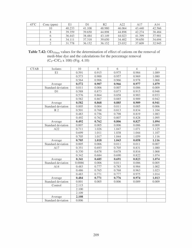
209
45oC Conc (ppm) E1 D1 R2 A22 A17 A14 10 40.233 41.108 48.980 46.064 43.440 42.566 8 39.359 39.650 44.898 44.898 42.274 38.484 6 36.443 38.484 43.149 44.023 41.399 37.901 4 34.111 37.318 39.650 34.402 39.650 34.694 2 31.778 36.152 36.152 23.032 37.609 32.945
Table 7.42: OD550nm values for the determination of effect of cations on the removal of medi-blue dye and the calculations for the percentage removal (C0−C/C0 x 100) (Fig. 4.10)
CTAB Isolates 10 8 6 4 2 E1 0.591 0.915 0.975 0.984 1.089 0.573 0.900 0.957 0.969 1.080 0.564 0.906 0.966 0.978 1.068 Average 0.572 0.907 0.966 0.977 1.079 Standard deviation 0.011 0.006 0.007 0.006 0.009 D1 0.588 0.873 0.873 0.915 0.948 0.576 0.864 0.858 0.903 0.933 0.582 0.867 0.885 0.909 0.942 Average 0.582 0.868 0.885 0.909 0.941 Standard deviation 0.005 0.004 0.011 0.005 0.006 R 2 0.501 0.768 0.813 0.834 1.104 0.483 0.756 0.798 0.819 1.083 0.492 0.762 0.807 0.828 1.095 Average 0.492 0.762 0.806 0.827 1.094 Standard deviation 0.007 0.005 0.006 0.006 0.009 A22 0.711 1.026 1.047 1.071 1.125 0.699 1.011 1.038 1.044 1.107 0.705 1.017 1.044 1.059 1.116 Average 0.705 1.018 1.043 0.058 1.116 Standard deviation 0.005 0.006 0.011 0.011 0.007 A17 0.351 0.693 0.705 0.831 1.080 0.330 0.678 0.678 0.816 1.068 0.342 0.684 0.690 0.822 1.074 Average 0.341 0.685 0.691 0.823 1.074 Standard deviation 0.0086 0.006 0.011 0.006 0.005 A14 0.483 0.777 0.783 0.984 1.002 0.486 0.765 0.768 0.963 1.023 0.483 0.771 0.777 0.975 1.014 Average 0.484 0.771 0.776 0.974 1.013 Standard deviation 0.001 0.005 0.006 0.009 0.009 Control 2.115 2.100 2.109 Average 2.108 Standard deviation 0.006

210
CTAB Conc (ppm) E1 D1 R2 A22 A17 A14 10 72.865 72.391 76.660 66.556 83.824 77.039 8 56.973 58.824 63.852 51.708 67.505 63.425 6 54.175 58.017 61.765 50.522 67.220 63.188 4 53.653 56.879 60.769 49.81 61.103 53.795 2 48.814 55.361 48.102 47.059 49.051 51.945
CaCl2 Isolates 10 8 6 4 2 E1 0.381 0.447 0.45 0.462 0.507 0.354 0.438 0.438 0.450 0.453 0.369 0.441 0.444 0.456 0.501 Average 0.368 0.442 0.444 0.456 0.487 Standard
deviation 0.011 0.004 0.005 0.005 0.024 D1 0.378 0.405 0.411 0.420 0.435 0.372 0.390 0.390 0.405 0.417 0.375 0.399 0.402 0.414 0.426 Average 0.375 0.398 0.401 0.413 0.1426 Standard
deviation 0.002 0.006 0.009 0.006 0.007 R 2 0.348 0.381 0.426 0.453 0.459 0.333 0.360 0.414 0.438 0.477 0.342 0.369 0.417 0.447 0.468 Average 0.341 0.37 0.419 0.446 0.468 Standard
deviation 0.006 0.009 0.005 0.006 0.007 A22 0.381 0.432 0.438 0.483 0.495 0.360 0.423 0.423 0.471 0.486 0.372 0.429 0.432 0.477 0.501 Average 0.371 0.428 0.431 0.477 0.490 Standard
deviation 0.009 0.004 0.006 0.005 0.006 A17 0.357 0.435 0.441 0.477 0.501 0.348 0.438 0.447 0.468 0.489 0.351 0.438 0.444 0.474 0.495 Average 0.352 0.473 0.444 0.473 0.495 Standard
deviation 0.004 0.001 0.002 0.003 0.005 A14 0.333 0.417 0.423 0.450 0.489 0.318 0.396 0.411 0.444 0.477 0.324 0.405 0.417 0.447 0.483 Average 0.325 0.406 0.417 0.447 0.483 Standard
deviation 0.006 0.009 0.005 0.002 0.005 Control 0.747 0.735 0.741 Average 0.741 Standard
deviation 0.005

211
CaCl2 Conc (ppm) E1 D1 R2 A22 A17 A14 10 50.337 49.393 53.981 49.933 52.497 56.140 8 40.351 46.289 50.067 42.240 41.026 45.209 6 40.081 45.884 43.455 41.835 40.081 43.725 4 38.462 44.265 39.811 35.628 36.167 39.676 2 34.278 42.510 36.842 33.873 33.198 34.818
MnCl2 Isolates 10 8 6 4 2
E1 0.003 0.015 0.027 0.057 0.069 0 0.006 0.012 0.045 0.06 0 0.012 0.018 0.051 0.06 Average 0.001 0.011 0.019 0.051 0.065 Standard
deviation 0.001 0.004 0.006 0.005 0.004 D1 0.030 0.048 0.054 0.051 0.057 0.045 0.036 0.045 0.057 0.066 0.039 0.042 0.051 0.054 0.060 Average 0.038 0.042 0.05 0.054 0.061 Standard
deviation 0.006 0.005 0.004 0.002 0.004 R 2 0.003 0.018 0.036 0.039 0.051 0.024 0.021 0.033 0.045 0.063 0.015 0.021 0.033 0.039 0.057 Average 0.014 0.020 0.034 0.041 0.057 Standard
deviation 0.009 0.001 0.001 0.003 0.005 A22 0.021 0.030 0.060 0.06 0.084 0.036 0.033 0.069 0.075 0.075 0.030 0.030 0.063 0.069 0.078 Average 0.029 0.031 0.064 0.068 0.079 Standard
deviation 0.006 0.001 0.004 0.006 0.004 A17 0.018 0.051 0.069 0.069 0.105 0.006 0.063 0.054 0.075 0.078 0.012 0.060 0.06 0.072 0.093 Average 0.012 0.058 0.061 0.072 0.092 Standard
deviation 0.005 0.005 0.006 0.002 0.011 A14 0.006 0.042 0.045 0.039 0.057 0.015 0.024 0.030 0.039 0.045 0.009 0.033 0.039 0.042 0.051 Average 0.010 0.033 0.038 0.04 0.051 Standard
deviation 0.004 0.004 0.006 0.001 0.005 Control 0.246 0.231 0.237 Average 0.238 Standard
deviation 0.006
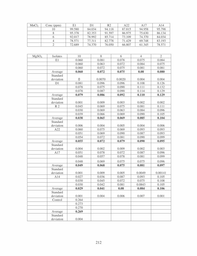
212
MnCl2 Conc (ppm) E1 D1 R2 A22 A17 A14 10 99.580 84.034 94.118 87.815 94.958 95.798 8 95.378 82.353 91.597 86.975 75.630 86.134 6 92.017 78.992 85.714 73.109 74.370 84.034 4 78.571 77.311 82.778 71.429 69.748 83.193 2 72.689 74.370 76.050 66.807 61.345 78.571
MgSO4 Isolates 10 8 6 4 2 E1 0.060 0.081 0.078 0.075 0.084 0.060 0.063 0.072 0.084 0.075 0.060 0.072 0.075 0.081 0.081 Average 0.060 0.072 0.075 0.08 0.080 Standard
deviation 0 0.0070 0.0020 0.004 0.004 D1 0.081 0.096 0.096 0.108 0.126 0.078 0.075 0.090 0.111 0.132 0.078 0.087 0.090 0.114 0.129 Average 0.079 0.086 0.092 0.110 0.129 Standard
deviation 0.001 0.009 0.003 0.002 0.002 R 2 0.045 0.069 0.075 0.081 0.111 0.030 0.069 0.063 0.084 0.096 0.039 0.066 0.069 0.090 0.105 Average 0.038 0.065 0.069 0.085 0.104 Standard
deviation 0.006 0.004 0.005 0.004 0.006 A22 0.060 0.075 0.069 0.093 0.093 0.051 0.069 0.090 0.087 0.093 0.054 0.072 0.081 0.090 0.099 Average 0.055 0.072 0.079 0.090 0.095 Standard
deviation 0.004 0.002 0.009 0.002 0.003 A17 0.051 0.078 0.072 0.087 0.096 0.048 0.057 0.078 0.081 0.099 0.048 0.069 0.075 0.075 0.096 Average 0.049 0.068 0.075 0.081 0.097 Standard
deviation 0.001 0.009 0.005 0.0049 0.00141 A14 0.027 0.036 0.087 0.093 0.105 0.030 0.045 0.072 0.075 0.108 0.030 0.042 0.081 0.0843 0.105 Average 0.029 0.041 0.08 0.084 0.106 Standard
deviation 0.001 0.004 0.006 0.007 0.001 Control 0.264 0.273 0.270 Average 0.269 Standard
deviation 0.004
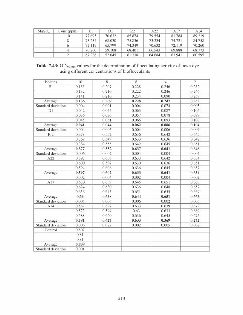
213
MgSO4 Conc (ppm) E1 D1 R2 A22 A17 A14 10 77.695 70.632 85.874 79.554 81.784 89.219 8 73.234 68.030 75.836 73.234 74.721 84.758 6 72.119 65.799 74.349 70.632 72.119 70.260 4 70.260 59.108 68.401 66.543 69.888 68.773 2 67.286 52.045 61.338 64.684 63.941 60.595
Table 7.43: OD550nm values for the determination of flocculating activity of fawn dye using different concentrations of bioflocculants
Isolates 10 8 6 4 2 E1 0.135 0.207 0.228 0.246 0.252
0.132 0.210 0.222 0.246 0.246 0.141 0.210 0.234 0.090 0.258
Average 0.136 0.209 0.228 0.247 0.252 Standard deviation 0.004 0.001 0.004 0.074 0.005
D1 0.042 0.045 0.063 0.087 0.105 0.036 0.036 0.057 0.078 0.099 0.045 0.051 0.066 0.093 0.108
Average 0.041 0.044 0.062 0.086 0.104 Standard deviation 0.004 0.006 0.004 0.006 0.004
R 2 0.378 0.552 0.636 0.642 0.645 0.369 0.549 0.633 0.636 0.642 0.384 0.555 0.642 0.645 0.651
Average 0.377 0.552 0.637 0.641 0.646 Standard deviation 0.006 0.002 0.004 0.004 0.004
A22 0.597 0.603 0.633 0.642 0.654 0.600 0.597 0.630 0.636 0.651 0.594 0.606 0.636 0.645 0.657
Average 0.597 0.602 0.633 0.641 0.654 0.002 0.004 0.002 0.004 0.002
A17 0.630 0.639 0.645 0.651 0.663 0.624 0.630 0.636 0.648 0.657 0.636 0.645 0.651 0.654 0.669
Average 0.63 0.638 0.644 0.651 0.663 Standard deviation 0.005 0.006 0.006 0.002 0.005
A14 0.582 0.627 0.633 0.639 0.672 0.573 0.594 0.63 0.633 0.669 0.588 0.660 0.636 0.645 0.675
Average 0.581 0.627 0.633 0.369 0.272 Standard deviation 0.006 0.027 0.002 0.005 0.002
Control 0.807 0.81 0.81
Average 0.809 Standard deviation 0.001

214
Table 7.44: Percentage removal (C0−C/C0 x 100) of fawn dye using different concentrations of flocculants as derived from Table 7.43 (Fig. 4.11)
Conc (ppm) E1 D1 R2 A22 A17 A14 10 83.189 94.932 53.399 26.205 22.126 28.183 8 74.166 94.561 31.768 25.587 21.137 22.467 6 71.817 92.336 21.261 21.755 20.396 21.755 4 69.468 89.369 20.766 20.766 19.530 21.014 2 68.850 87.145 20.148 19.159 18.047 16.934
Table 7.45: Flocculating activity of fawn dye as derived from Table 7.43 using an equation for flocculating activity in Section 4.2.3 (Fig. 4.12)
Isolate Flocculating activity Standard deviation E1 14.158 0.198 D1 4.468 0.152 R2 17.613 0.369
A22 73.368 0.215 A17 146.413 0.166 A14 56.011 0.200
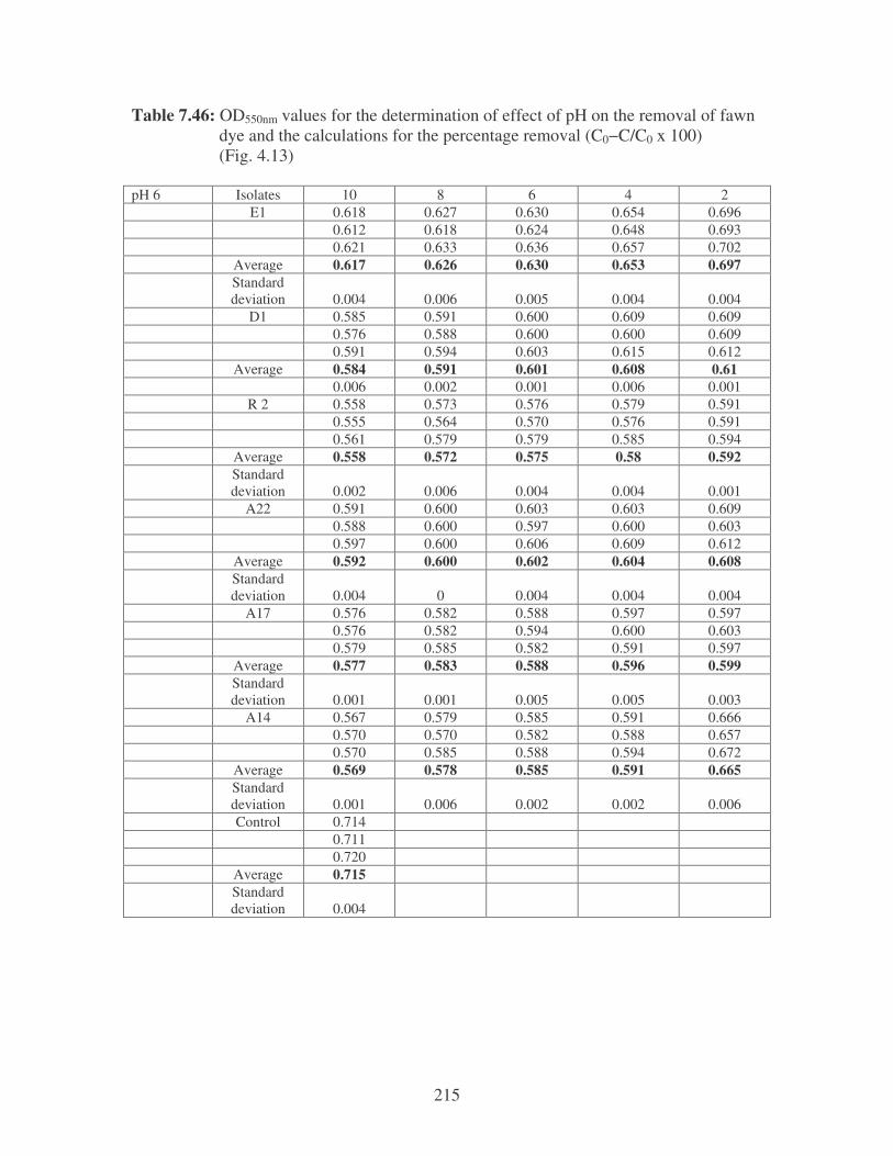
215
Table 7.46: OD550nm values for the determination of effect of pH on the removal of fawn dye and the calculations for the percentage removal (C0−C/C0 x 100) (Fig. 4.13) pH 6 Isolates 10 8 6 4 2 E1 0.618 0.627 0.630 0.654 0.696 0.612 0.618 0.624 0.648 0.693 0.621 0.633 0.636 0.657 0.702 Average 0.617 0.626 0.630 0.653 0.697 Standard
deviation 0.004 0.006 0.005 0.004 0.004 D1 0.585 0.591 0.600 0.609 0.609 0.576 0.588 0.600 0.600 0.609 0.591 0.594 0.603 0.615 0.612 Average 0.584 0.591 0.601 0.608 0.61 0.006 0.002 0.001 0.006 0.001 R 2 0.558 0.573 0.576 0.579 0.591 0.555 0.564 0.570 0.576 0.591 0.561 0.579 0.579 0.585 0.594 Average 0.558 0.572 0.575 0.58 0.592 Standard
deviation 0.002 0.006 0.004 0.004 0.001 A22 0.591 0.600 0.603 0.603 0.609 0.588 0.600 0.597 0.600 0.603 0.597 0.600 0.606 0.609 0.612 Average 0.592 0.600 0.602 0.604 0.608 Standard
deviation 0.004 0 0.004 0.004 0.004 A17 0.576 0.582 0.588 0.597 0.597 0.576 0.582 0.594 0.600 0.603 0.579 0.585 0.582 0.591 0.597 Average 0.577 0.583 0.588 0.596 0.599 Standard
deviation 0.001 0.001 0.005 0.005 0.003 A14 0.567 0.579 0.585 0.591 0.666 0.570 0.570 0.582 0.588 0.657 0.570 0.585 0.588 0.594 0.672 Average 0.569 0.578 0.585 0.591 0.665 Standard
deviation 0.001 0.006 0.002 0.002 0.006 Control 0.714 0.711 0.720 Average 0.715 Standard
deviation 0.004
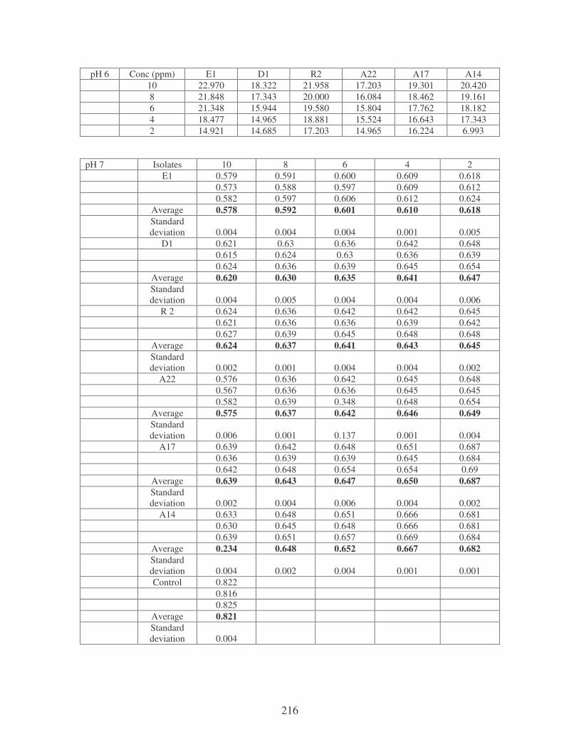
216
pH 6 Conc (ppm) E1 D1 R2 A22 A17 A14 10 22.970 18.322 21.958 17.203 19.301 20.420 8 21.848 17.343 20.000 16.084 18.462 19.161 6 21.348 15.944 19.580 15.804 17.762 18.182 4 18.477 14.965 18.881 15.524 16.643 17.343 2 14.921 14.685 17.203 14.965 16.224 6.993
pH 7 Isolates 10 8 6 4 2 E1 0.579 0.591 0.600 0.609 0.618 0.573 0.588 0.597 0.609 0.612 0.582 0.597 0.606 0.612 0.624 Average 0.578 0.592 0.601 0.610 0.618 Standard
deviation 0.004 0.004 0.004 0.001 0.005 D1 0.621 0.63 0.636 0.642 0.648 0.615 0.624 0.63 0.636 0.639 0.624 0.636 0.639 0.645 0.654 Average 0.620 0.630 0.635 0.641 0.647 Standard
deviation 0.004 0.005 0.004 0.004 0.006 R 2 0.624 0.636 0.642 0.642 0.645 0.621 0.636 0.636 0.639 0.642 0.627 0.639 0.645 0.648 0.648 Average 0.624 0.637 0.641 0.643 0.645 Standard
deviation 0.002 0.001 0.004 0.004 0.002 A22 0.576 0.636 0.642 0.645 0.648 0.567 0.636 0.636 0.645 0.645 0.582 0.639 0.348 0.648 0.654 Average 0.575 0.637 0.642 0.646 0.649 Standard
deviation 0.006 0.001 0.137 0.001 0.004 A17 0.639 0.642 0.648 0.651 0.687 0.636 0.639 0.639 0.645 0.684 0.642 0.648 0.654 0.654 0.69 Average 0.639 0.643 0.647 0.650 0.687 Standard
deviation 0.002 0.004 0.006 0.004 0.002 A14 0.633 0.648 0.651 0.666 0.681 0.630 0.645 0.648 0.666 0.681 0.639 0.651 0.657 0.669 0.684 Average 0.234 0.648 0.652 0.667 0.682 Standard
deviation 0.004 0.002 0.004 0.001 0.001 Control 0.822 0.816 0.825 Average 0.821 Standard
deviation 0.004
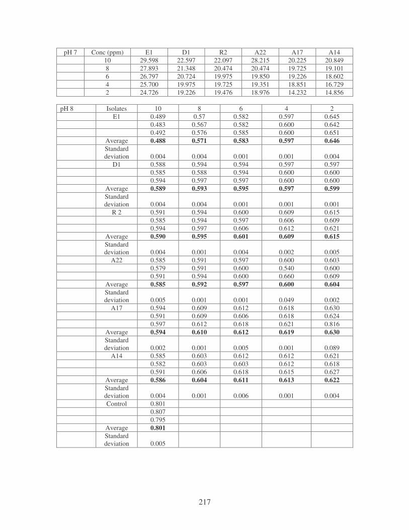
217
pH 7 Conc (ppm) E1 D1 R2 A22 A17 A14 10 29.598 22.597 22.097 28.215 20.225 20.849 8 27.893 21.348 20.474 20.474 19.725 19.101 6 26.797 20.724 19.975 19.850 19.226 18.602 4 25.700 19.975 19.725 19.351 18.851 16.729 2 24.726 19.226 19.476 18.976 14.232 14.856
pH 8 Isolates 10 8 6 4 2 E1 0.489 0.57 0.582 0.597 0.645 0.483 0.567 0.582 0.600 0.642 0.492 0.576 0.585 0.600 0.651 Average 0.488 0.571 0.583 0.597 0.646 Standard
deviation 0.004 0.004 0.001 0.001 0.004 D1 0.588 0.594 0.594 0.597 0.597 0.585 0.588 0.594 0.600 0.600 0.594 0.597 0.597 0.600 0.600 Average 0.589 0.593 0.595 0.597 0.599 Standard
deviation 0.004 0.004 0.001 0.001 0.001 R 2 0.591 0.594 0.600 0.609 0.615 0.585 0.594 0.597 0.606 0.609 0.594 0.597 0.606 0.612 0.621 Average 0.590 0.595 0.601 0.609 0.615 Standard
deviation 0.004 0.001 0.004 0.002 0.005 A22 0.585 0.591 0.597 0.600 0.603 0.579 0.591 0.600 0.540 0.600 0.591 0.594 0.600 0.660 0.609 Average 0.585 0.592 0.597 0.600 0.604 Standard
deviation 0.005 0.001 0.001 0.049 0.002 A17 0.594 0.609 0.612 0.618 0.630 0.591 0.609 0.606 0.618 0.624 0.597 0.612 0.618 0.621 0.816 Average 0.594 0.610 0.612 0.619 0.630 Standard
deviation 0.002 0.001 0.005 0.001 0.089 A14 0.585 0.603 0.612 0.612 0.621 0.582 0.603 0.603 0.612 0.618 0.591 0.606 0.618 0.615 0.627 Average 0.586 0.604 0.611 0.613 0.622 Standard
deviation 0.004 0.001 0.006 0.001 0.004 Control 0.801 0.807 0.795 Average 0.801 Standard
deviation 0.005

218
pH 8 Conc (ppm) E1 D1 R2 A22 A17 A14 10 31.748 28.258 28.136 28.745 27.649 28.624 8 20.140 27.771 27.771 27.893 25.700 26.431 6 18.462 27.527 27.797 27.283 25.457 25.579 4 16.503 27.284 25.822 26.918 24.604 25.335 2 9.650 27.040 25.091 26.431 23.264 24.239
pH 9 Isolates 10 8 6 4 2
E1 0.345 0.348 0.354 0.366 0.387 0.342 0.342 0.354 0.366 0.378 0.351 0.354 0.357 0.372 0.393 Average 0.346 0.348 0.355 0.368 0.386 Standard
deviation 0.004 0.005 0.001 0.003 0.006 D1 0.348 0.354 0.357 0.360 0.366 0.342 0.351 0.351 0.357 0.363 0.354 0.357 0.36 0.366 0.372 Average 0.348 0.354 0.356 0.361 0.367 Standard
deviation 0.005 0.002 0.004 0.004 0.004 R 2 0.435 0.450 0.453 0.453 0.462 0.432 0.444 0.444 0.453 0.456 0.441 0.453 0.459 0.456 0.465 Average 0.436 0.449 0.452 0.454 0.461 Standard
deviation 0.004 0.004 0.006 0.001 0.004 A22 0.447 0.456 0.465 0.471 0.501 0.444 0.453 0.459 0.465 0.498 0.450 0.459 0.471 0.474 0.507 Average 0.447 0.456 0.465 0.470 0.502 Standard
deviation 0.002 0.002 0.005 0.004 0.004 A14 0.348 0.351 0.456 0.468 0.510 0.348 0.348 0.450 0.468 0.504 0.351 0.354 0.462 0.471 0.516 Average 0.349 0.351 0.456 0.469 0.51 Standard
deviation 0.001 0.002 0.005 0.001 0.005 A17 0.351 0.366 0.372 0.399 0.405 0.348 0.363 0.366 0.396 0.405 0.357 0.372 0.375 0.402 0.408 Average 0.352 0.367 0.371 0.399 0.406 Standard
deviation 0.004 0.004 0.004 0.002 0.001 Control 0.825 0.822 0.828 Average 0.825 Standard
deviation 0.002

219
pH 9 Conc (ppm) E1 D1 R2 A22 A17 A14 10 58.061 57.818 47.152 45.818 57.333 57.697 8 57.818 57.091 45.576 44.727 55.515 57.455 6 56.970 56.848 45.212 44.848 55.030 44.727 4 55.394 56.242 44.970 43.030 51.636 43.152 2 53.212 55.515 44.121 39.152 50.788 38.182
pH 10 Isolates 10 8 6 4 2 E1 0.312 0.321 0.342 0.348 0.366 0.309 0.312 0.339 0.348 0.357 0.315 0.327 0.345 0.351 0.372 Average 0.312 0.320 0.342 0.349 0.365 Standard
deviation 0.002 0.006 0.002 0.001 0.006 D1 0.339 0.348 0.354 0.372 0.387 0.330 0.348 0.348 0.366 0.384 0.345 0.351 0.357 0.375 0.390 Average 0.338 0.349 0.353 0.371 0.387 Standard
deviation 0.006 0.001 0.004 0.004 0.002 R 2 0.318 0.342 0.348 0.351 0.357 0.315 0.339 0.342 0.348 0.351 0.321 0.345 0.351 0.357 0.36 Average 0.318 0.342 0.347 0.352 0.356 Standard
deviation 0.002 0.002 0.004 0.004 0.004 A22 0.339 0.363 0.366 0.366 0.372 0.333 0.354 0.357 0.363 0.366 0.345 0.369 0.372 0.372 0.375 Average 0.339 0.362 0.365 0.367 0.371 Standard
deviation 0.005 0.006 0.006 0.004 0.004 A17 0.354 0.360 0.363 0.369 0.384 0.354 0.351 0.354 0.363 0.381 0.357 0.366 0.369 0.372 0.390 Average 0.355 0.359 0.362 0.368 0.385 Standard
deviation 0.001 0.006 0.006 0.004 0.004 A14 0.354 0.357 0.360 0.366 0.369 0.348 0.351 0.357 0.363 0.363 0.357 0.363 0.363 0.369 0.375 Average 0.353 0.357 0.36 0.366 0.369 Standard
deviation 0.004 0.005 0.002 0.002 0.005 Control 0.831 0.825 0.837 Average 0.831 Standard
deviation 0.005

220
pH 10 Conc (ppm) E1 D1 R2 A22 A17 A14 10 62.455 59.326 61.733 59.206 57.280 57.521 8 61.492 58.002 58.845 56.438 56.799 57.040 6 58.845 56.799 58.243 56.077 56.438 56.979 4 58.002 55.355 57.641 55.836 55.716 55.957 2 56.077 53.430 57.160 55.355 53.670 55.596
Table 7.47: OD550nm values for the determination of effect of temperature on the removal fawn dye and the calculations for the percentage removal (C0−C/C0 x 100) (Fig. 4.14)
28oC Isolates 10 8 6 4 2 E1 0.639 0.645 0.648 0.651 0.657 0.633 0.642 0.642 0.645 0.654 0.645 0.648 0.651 0.657 0.663 Average 0.639 0.645 0.647 0.651 0.658 Standard deviation 0.005 0.002 0.004 0.005 0.004 D1 0.642 0.651 0.654 0.657 0.663 0.642 0.648 0.654 0.687 0.657 0.645 0.657 0.657 0.633 0.669 Average 0.643 0.652 0.655 0.659 0.663 Standard deviation 0.001 0.004 0.001 0.020 0.0045 R 2 0.645 0.648 0.657 0.660 0.663 0.639 0.648 0.654 0.657 0.654 0.648 0.651 0.660 0.663 0.669 Average 0.644 0.649 0.657 0.66 0.662 Standard deviation 0.004 0.001 0.002 0.002 0.006 A22 0.642 0.648 0.651 0.660 0.669 0.636 0.642 0.648 0.657 0.672 0.645 0.651 0.654 0.663 0.669 Average 0.641 0.647 0.651 0.660 0.670 Standard deviation 0.004 0.004 0.002 0.002 0.001 A17 0.657 0.66 0.663 0.666 0.702 0.651 0.657 0.657 0.660 0.699 0.660 0.663 0.669 0.669 0.705 Average 0.656 0.660 0.663 0.665 0.702 Standard deviation 0.004 0.002 0.005 0.004 0.002 A14 0.546 0.612 0.627 0.657 0.666 0.543 0.606 0.627 0.654 0.660 0.552 0.615 0.63 0.660 0.669 Average 0.547 0.611 0.629 0.628 0.665 Standard deviation 0.004 0.004 0.001 0.003 0.004 Control 0.858 0.846 0.867 Average 0.857 Standard deviation 0.009
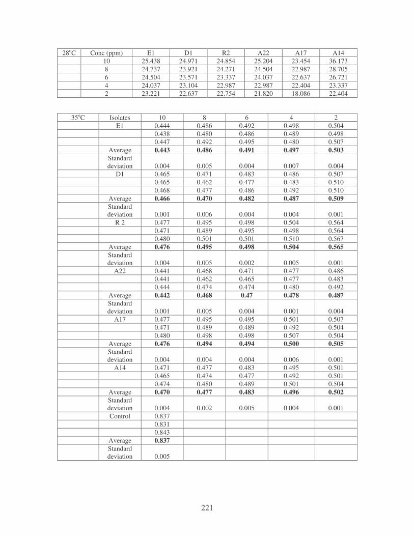
221
28oC Conc (ppm) E1 D1 R2 A22 A17 A14 10 25.438 24.971 24.854 25.204 23.454 36.173 8 24.737 23.921 24.271 24.504 22.987 28.705 6 24.504 23.571 23.337 24.037 22.637 26.721 4 24.037 23.104 22.987 22.987 22.404 23.337 2 23.221 22.637 22.754 21.820 18.086 22.404
35oC Isolates 10 8 6 4 2 E1 0.444 0.486 0.492 0.498 0.504 0.438 0.480 0.486 0.489 0.498 0.447 0.492 0.495 0.480 0.507 Average 0.443 0.486 0.491 0.497 0.503 Standard
deviation 0.004 0.005 0.004 0.007 0.004 D1 0.465 0.471 0.483 0.486 0.507 0.465 0.462 0.477 0.483 0.510 0.468 0.477 0.486 0.492 0.510 Average 0.466 0.470 0.482 0.487 0.509 Standard
deviation 0.001 0.006 0.004 0.004 0.001 R 2 0.477 0.495 0.498 0.504 0.564 0.471 0.489 0.495 0.498 0.564 0.480 0.501 0.501 0.510 0.567 Average 0.476 0.495 0.498 0.504 0.565 Standard
deviation 0.004 0.005 0.002 0.005 0.001 A22 0.441 0.468 0.471 0.477 0.486 0.441 0.462 0.465 0.477 0.483 0.444 0.474 0.474 0.480 0.492 Average 0.442 0.468 0.47 0.478 0.487 Standard
deviation 0.001 0.005 0.004 0.001 0.004 A17 0.477 0.495 0.495 0.501 0.507 0.471 0.489 0.489 0.492 0.504 0.480 0.498 0.498 0.507 0.504 Average 0.476 0.494 0.494 0.500 0.505 Standard
deviation 0.004 0.004 0.004 0.006 0.001 A14 0.471 0.477 0.483 0.495 0.501 0.465 0.474 0.477 0.492 0.501 0.474 0.480 0.489 0.501 0.504 Average 0.470 0.477 0.483 0.496 0.502 Standard
deviation 0.004 0.002 0.005 0.004 0.001 Control 0.837 0.831 0.843 Average 0.837 Standard
deviation 0.005

222
35oC Conc (ppm) E1 D1 R2 A22 A17 A14 10 47.073 44.325 43.130 47.192 43.130 43.847 8 41.935 43.847 40.860 44.086 40.980 43.010 6 41.338 42.413 40.502 43.847 40.502 42.294 4 40.621 41.816 39.785 42.891 40.263 40.741 2 39.904 39.188 32.497 41.816 39.665 40.024
40oC Isolates 10 8 6 4 2
E1 0.315 0.324 0.429 0.429 0.444 0.321 0.324 0.435 0.444 0.447 0.318 0.324 0.432 0.438 0.444 Average 0.318 0.326 0.432 0.437 0.445 Standard
deviation 0.002 0 0.002 0.006 0.001 D1 0.420 0.432 0.435 0.462 0.492 0.435 0.410 0.447 0.450 0.498 0.426 0.438 0.441 0.453 0.492 Average 0.427 0.437 0.441 0.454 0.494 Standard
deviation 0.006 0.0120 0.005 0.005 0.003 R 2 0.435 0.438 0.450 0.450 0.492 0.444 0.450 0.459 0.465 0.498 0.441 0.444 0.453 0.459 0.495 Average 0.440 0.444 0.454 0.458 0.495 Standard
deviation 0.004 0.005 0.004 0.006 0.002 A22 0.306 0.315 0.321 0.444 0.444 0.312 0.327 0.336 0.438 0.447 0.309 0.321 0.330 0.441 0.444 Average 0.309 0.321 0.329 0.441 0.445 Standard
deviation 0.002 0.005 0.006 0.002 0.001 A17 0.432 0.432 0.540 0.555 0.573 0.438 0.447 0.549 0.561 0.582 0.435 0.441 0.546 0.558 0.576 Average 0.435 0.440 0.545 0.558 0.577 Standard
deviation 0.002 0.006 0.004 0.002 0.004 A14 0.420 0.441 0.441 0.47 0.483 0.429 0.444 0.45 0.453 0.471 0.423 0.441 0.447 0.45 0.477 Average 0.424 0.442 0.446 0.45 0.477 Standard
deviation 0.004 0.001 0.004 0.008 0.005 Control 0.825 0.828 0.825 Average 0.826 Standard
deviation 0.001
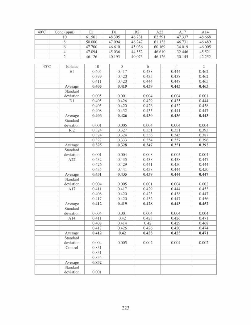
223
40oC Conc (ppm) E1 D1 R2 A22 A17 A14 10 61.501 48.305 46.731 62.591 47.337 48.668 8 50.000 47.094 46.247 61.138 46.731 46.489 6 47.700 46.610 45.036 60.169 34.019 46.005 4 47.094 45.036 44.552 46.610 32.446 45.521 2 46.126 40.193 40.073 46.126 30.145 42.252
45oC Isolates 10 8 6 4 2
E1 0.405 0.417 0.438 0.444 0.462 0.399 0.420 0.435 0.438 0.462 0.411 0.420 0.444 0.447 0.465 Average 0.405 0.419 0.439 0.443 0.463 Standard
deviation 0.005 0.001 0.004 0.004 0.001 D1 0.405 0.426 0.429 0.435 0.444 0.405 0.420 0.426 0.432 0.438 0.408 0.432 0.435 0.441 0.447 Average 0.406 0.426 0.430 0.436 0.443 Standard
deviation 0.001 0.005 0.004 0.004 0.004 R 2 0.324 0.327 0.351 0.351 0.393 0.324 0.324 0.336 0.345 0.387 0.327 0.333 0.354 0.357 0.396 Average 0.325 0.328 0.347 0.351 0.392 Standard
deviation 0.001 0.004 0.008 0.005 0.004 A22 0.432 0.435 0.438 0.438 0.447 0.426 0.429 0.441 0.450 0.444 0.435 0.441 0.438 0.444 0.450 Average 0.431 0.435 0.439 0.444 0.447 Standard
deviation 0.004 0.005 0.001 0.004 0.002 A17 0.411 0.417 0.429 0.444 0.453 0.408 0.420 0.423 0.438 0.447 0.417 0.420 0.432 0.447 0.456 Average 0.412 0.419 0.428 0.443 0.452 Standard
deviation 0.004 0.001 0.004 0.004 0.004 A14 0.411 0.42 0.423 0.426 0.471 0.408 0.414 0.42 0.429 0.468 0.417 0.426 0.426 0.420 0.474 Average 0.412 0.42 0.423 0.425 0.471 Standard
deviation 0.004 0.005 0.002 0.004 0.002 Control 0.831 0.831 0.834 Average 0.832 Standard
deviation 0.001
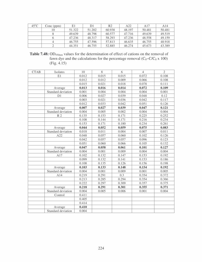
224
45oC Conc (ppm) E1 D1 R2 A22 A17 A14 10 51.322 51.202 60.938 48.197 50.481 50.481 8 49.639 48.798 60.577 47.716 49.639 49.519 6 47.236 48.317 58.293 47.236 48.558 49.159 4 46.755 47.596 57.813 46.635 46.755 48.918 2 44.351 46.755 52.885 46.274 45.673 43.389
Table 7.48: OD550nm values for the determination of effect of cations on the removal of fawn dye and the calculations for the percentage removal (C0−C/C0 x 100) (Fig. 4.15)
CTAB Isolates 10 8 6 4 2 E1 0.012 0.015 0.015 0.072 0.108 0.012 0.012 0.009 0.066 0.108 0.015 0.021 0.018 0.078 0.111 Average 0.013 0.016 0.014 0.072 0.109 Standard deviation 0.001 0.004 0.004 0.004 0.001 D1 0.006 0.027 0.039 0.048 0.12 0.003 0.021 0.036 0.042 0.117 0.012 0.033 0.042 0.051 0.126 Average 0.007 0.027 0.039 0.047 0.121 Standard deviation 0.004 0.005 0.002 0.004 0.004 R 2 0.135 0.153 0.171 0.225 0.252 0.108 0.144 0.171 0.216 0.234 0.153 0.171 0.180 0.234 0.261 Average 0.044 0.052 0.059 0.075 0.083 Standard deviation 0.018 0.011 0.004 0.007 0.011 A22 0.048 0.057 0.060 0.102 0.126 0.042 0.057 0.057 0.096 0.123 0.051 0.060 0.066 0.105 0.132 Average 0.047 0.058 0.061 0.101 0.127 Standard deviation 0.004 0.001 0.009 0.004 0.004 A17 0.102 0.132 0.147 0.153 0.192 0.099 0.132 0.141 0.153 0.186 0.108 0.135 0.126 0.156 0.198 Average 0.103 0.133 0.148 0.154 0.192 Standard deviation 0.004 0.001 0.009 0.001 0.005 A14 0.219 0.291 0.3 0.354 0.372 0.213 0.285 0.294 0.354 0.366 0.222 0.297 0.309 0.357 0.375 Average 0.218 0.291 0.301 0.355 0.371 Standard deviation 0.004 0.005 0.006 0.001 0.004 Control 0.411 0.405 0.414 Average 0.410 Standard deviation 0.004
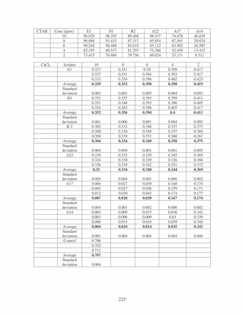
225
CTAB Conc (ppm) E1 D1 R2 A22 A17 A14 10 96.829 98.293 89.268 88.537 74.878 46.829 8 96.098 93.415 87.317 85.854 67.561 29.024 6 90.244 90.488 85.610 85.122 63.902 26.585 4 82.195 88.537 81.707 75.366 92.439 13.415 2 73.415 70.488 79.756 69.024 53.171 9.512
CaCl2 Isolates 10 8 6 4 2
E1 0.327 0.351 0.39 0.399 0.417 0.327 0.351 0.384 0.393 0.417 0.333 0.354 0.396 0.402 0.423 Average 0.329 0.352 0.390 0.398 0.419 Standard
deviation 0.003 0.001 0.005 0.004 0.003 D1 0.351 0.357 0.393 0.399 0.411 0.351 0.348 0.393 0.396 0.405 0.354 0.363 0.396 0.405 0.417 Average 0.352 0.356 0.394 0.4 0.411 Standard
deviation 0.001 0.006 0.001 0.004 0.005 R 2 0.303 0.333 0.348 0.357 0.375 0.300 0.330 0.348 0.357 0.369 0.309 0.339 0.351 0.360 0.381 Average 0.304 0.334 0.349 0.358 0.375 Standard
deviation 0.004 0.004 0.001 0.001 0.005 A22 0.330 0.333 0.339 0.345 0.369 0.324 0.330 0.339 0.336 0.366 0.336 0.339 0.342 0.351 0.372 Average 0.33 0.334 0.340 0.344 0.369 Standard
deviation 0.005 0.004 0.001 0.006 0.002 A17 0.006 0.027 0.039 0.168 0.174 0.003 0.027 0.036 0.159 0.171 0.012 0.030 0.042 0.174 0.177 Average 0.007 0.028 0.039 0.167 0.174 Standard
deviation 0.004 0.001 0.002 0.006 0.002 A14 0.003 0.009 0.015 0.036 0.342 0.003 0.006 0.009 0.03 0.339 0.006 0.015 0.018 0.039 0.348 Average 0.004 0.010 0.014 0.035 0.343 Standard
deviation 0.001 0.004 0.004 0.004 0.004 Control 0.708 0.702 0.711 Average 0.707 Standard
deviation 0.004

226
CaCl2 Conc (ppm) E1 D1 R2 A22 A17 A14 10 53.465 50.212 57.001 53.324 99.010 99.434 8 50.212 49.646 52.646 52.758 96.040 98.586 6 44.837 44.272 50.636 51.909 94.484 98.020 4 43.706 43.423 49.364 51.344 76.379 95.050 2 40.736 41.867 46.959 47.808 75.389 93.918
MnCl2 Isolates 10 8 6 4 2
E1 0.120 0.141 0.159 0.156 0.195 0.114 0.135 0.153 0.147 0.189 0.126 0.144 0.162 0.162 0.198 Average 0.120 0.140 0.158 0.155 0.194 Standard
deviation 0.005 0.004 0.004 0.006 0.004 D1 0.105 0.120 0.144 0.150 0.189 0.102 0.117 0.138 0.141 0.189 0.108 0.126 0.147 0.156 0.192 Average 0.105 0.121 0.143 0.149 0.190 Standard
deviation 0.003 0.004 0.004 0.006 0.001 R 2 0.129 0.141 0.153 0.621 0.168 0.120 0.141 0.153 0.612 0.162 0.135 0.144 0.156 0.627 0.171 Average 0.128 0.142 0.154 0.62 0.167 Standard
deviation 0.006 0.001 0.001 0.006 0.004 A22 0.138 0.153 0.162 0.168 0.261 0.138 0.150 0.156 0.165 0.258 0.141 0.159 0.165 0.174 0.264 Average 0.139 0.154 0.161 0.169 0.261 Standard
deviation 0.001 0.004 0.004 0.006 0.002 A17 0.123 0.156 0.177 0.198 0.207 0.120 0.153 0.174 0.198 0.204 0.129 0.162 0.18 0.201 0.210 Average 0.124 0.157 0.177 0.199 0.207 Standard
deviation 0.004 0.004 0.002 0.001 0.002 A14 0.087 0.126 0.141 0.144 0.159 0.090 0.120 0.141 0.144 0.153 0.090 0.129 0.147 0.147 0.165 Average 0.089 0.125 0.141 0.145 0.159 Standard
deviation 0.001 0.004 0.003 0.001 0.005 Control 0.531 0.540 0.522 Average 0.531 Standard
deviation 0.007

227
MnCl2 Conc (ppm) E1 D1 R2 A22 A17 A14 10 77.401 80.226 76.038 73.823 76.648 83.239 8 73.635 77.213 73.258 70.998 70.433 76.460 6 71.186 73.070 70.998 69.680 66.667 73.446 4 70.810 70.056 69.492 68.173 62.524 72.693 2 63.465 64.218 68.550 50.847 61.017 70.056
MgSO4 Isolates 10 8 6 4 2
E1 0.156 0.18 0.186 0.192 0.198 0.153 0.177 0.180 0.189 0.189 0.162 0.183 0.192 0.195 0.204 Average 0.157 0.18 0.186 0.192 0.197 Standard
deviation 0.004 0.002 0.005 0.002 0.006 D1 0.144 0.162 0.165 0.171 0.177 0.138 0.156 0.159 0.168 0.174 0.147 0.165 0.168 0.177 0.180 Average 0.143 0.161 0.164 0.172 0.177 Standard
deviation 0.004 0.004 0.004 0.003 0.002 R 2 0.141 0.147 0.171 0.192 0.201 0.135 0.144 0.168 0.189 0.198 0.144 0.153 0.177 0.195 0.204 Average 0.140 0.148 0.172 0.192 0.201 Standard
deviation 0.004 0.004 0.004 0.002 0.002 A22 0.141 0.429 0.168 0.186 0.210 0.135 0.153 0.162 0.180 0.210 0.144 0.165 0.171 0.192 0.213 Average 0.140 0.159 0.167 0.186 0.211 Standard
deviation 0.004 0.127 0.004 0.005 0.001 A17 0.162 0.171 0.177 0.183 0.234 0.156 0.165 0.174 0.183 0.231 0.165 0.177 0.183 0.186 0.24 Average 0.161 0.171 0.178 0.184 0.235 Standard
deviation 0.004 0.005 0.004 0.001 0.004 A14 0.174 0.183 0.192 0.192 0.195 0.165 0.183 0.186 0.189 0.195 0.180 0.186 0.195 0.198 0.198 Average 0.173 0.184 0.191 0.193 0.196 Standard
deviation 0.006 0.001 0.004 0.004 0.001 Control 0.543 0.537 0.546 Average 0.542 Standard
deviation 0.00374
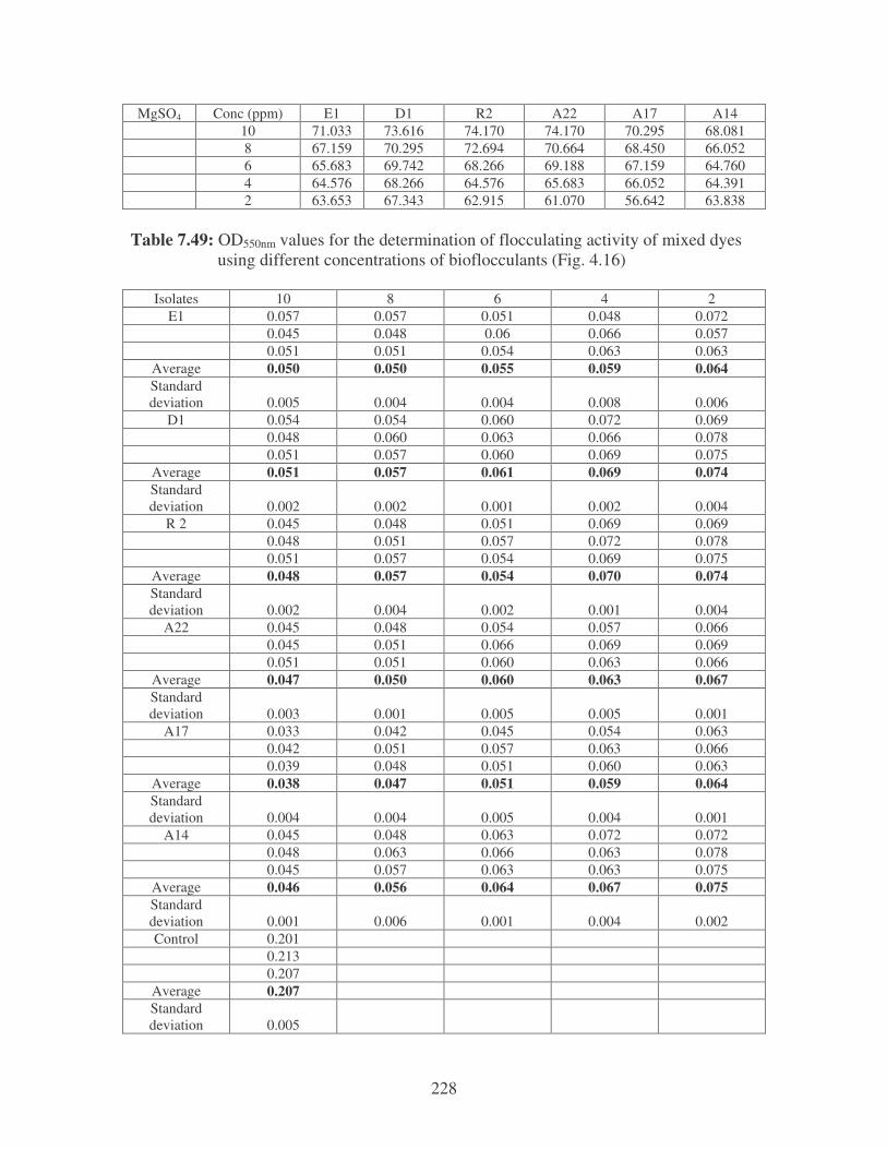
228
MgSO4 Conc (ppm) E1 D1 R2 A22 A17 A14 10 71.033 73.616 74.170 74.170 70.295 68.081 8 67.159 70.295 72.694 70.664 68.450 66.052 6 65.683 69.742 68.266 69.188 67.159 64.760 4 64.576 68.266 64.576 65.683 66.052 64.391 2 63.653 67.343 62.915 61.070 56.642 63.838
Table 7.49: OD550nm values for the determination of flocculating activity of mixed dyes using different concentrations of bioflocculants (Fig. 4.16)
Isolates 10 8 6 4 2 E1 0.057 0.057 0.051 0.048 0.072
0.045 0.048 0.06 0.066 0.057 0.051 0.051 0.054 0.063 0.063
Average 0.050 0.050 0.055 0.059 0.064 Standard deviation 0.005 0.004 0.004 0.008 0.006
D1 0.054 0.054 0.060 0.072 0.069 0.048 0.060 0.063 0.066 0.078 0.051 0.057 0.060 0.069 0.075
Average 0.051 0.057 0.061 0.069 0.074 Standard deviation 0.002 0.002 0.001 0.002 0.004
R 2 0.045 0.048 0.051 0.069 0.069 0.048 0.051 0.057 0.072 0.078 0.051 0.057 0.054 0.069 0.075
Average 0.048 0.057 0.054 0.070 0.074 Standard deviation 0.002 0.004 0.002 0.001 0.004
A22 0.045 0.048 0.054 0.057 0.066 0.045 0.051 0.066 0.069 0.069 0.051 0.051 0.060 0.063 0.066
Average 0.047 0.050 0.060 0.063 0.067 Standard deviation 0.003 0.001 0.005 0.005 0.001
A17 0.033 0.042 0.045 0.054 0.063 0.042 0.051 0.057 0.063 0.066 0.039 0.048 0.051 0.060 0.063
Average 0.038 0.047 0.051 0.059 0.064 Standard deviation 0.004 0.004 0.005 0.004 0.001
A14 0.045 0.048 0.063 0.072 0.072 0.048 0.063 0.066 0.063 0.078 0.045 0.057 0.063 0.063 0.075
Average 0.046 0.056 0.064 0.067 0.075 Standard deviation 0.001 0.006 0.001 0.004 0.002 Control 0.201
0.213 0.207
Average 0.207 Standard deviation 0.005
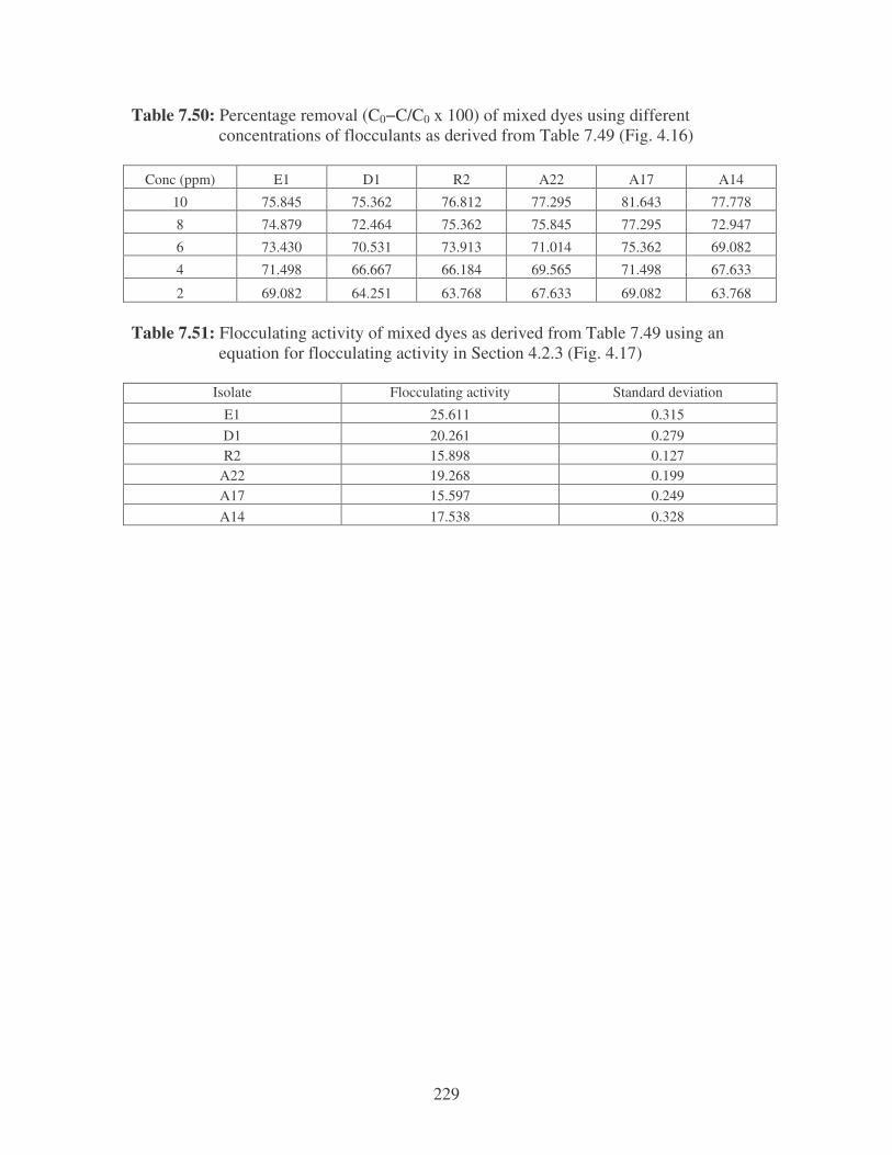
229
Table 7.50: Percentage removal (C0−C/C0 x 100) of mixed dyes using different concentrations of flocculants as derived from Table 7.49 (Fig. 4.16)
Conc (ppm) E1 D1 R2 A22 A17 A14
10 75.845 75.362 76.812 77.295 81.643 77.778
8 74.879 72.464 75.362 75.845 77.295 72.947
6 73.430 70.531 73.913 71.014 75.362 69.082
4 71.498 66.667 66.184 69.565 71.498 67.633
2 69.082 64.251 63.768 67.633 69.082 63.768 Table 7.51: Flocculating activity of mixed dyes as derived from Table 7.49 using an equation for flocculating activity in Section 4.2.3 (Fig. 4.17)
Isolate Flocculating activity Standard deviation
E1 25.611 0.315 D1 20.261 0.279 R2 15.898 0.127
A22 19.268 0.199 A17 15.597 0.249 A14 17.538 0.328
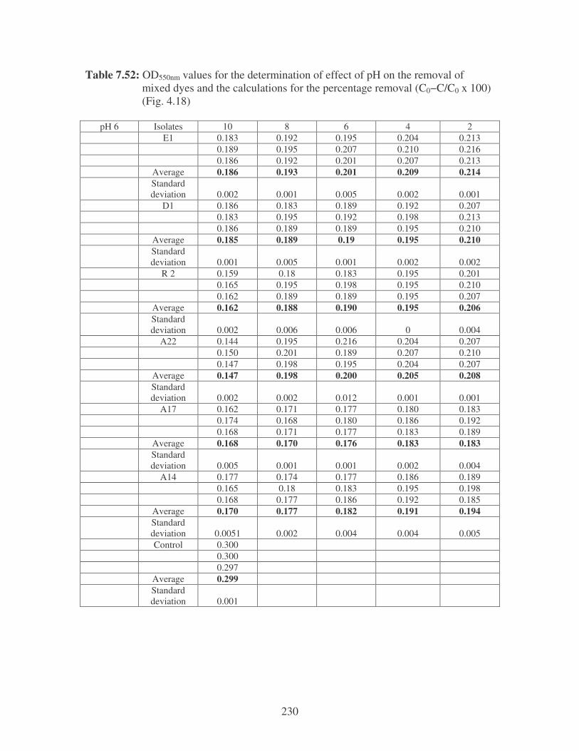
230
Table 7.52: OD550nm values for the determination of effect of pH on the removal of mixed dyes and the calculations for the percentage removal (C0−C/C0 x 100) (Fig. 4.18)
pH 6 Isolates 10 8 6 4 2 E1 0.183 0.192 0.195 0.204 0.213 0.189 0.195 0.207 0.210 0.216 0.186 0.192 0.201 0.207 0.213 Average 0.186 0.193 0.201 0.209 0.214 Standard
deviation 0.002 0.001 0.005 0.002 0.001 D1 0.186 0.183 0.189 0.192 0.207 0.183 0.195 0.192 0.198 0.213 0.186 0.189 0.189 0.195 0.210 Average 0.185 0.189 0.19 0.195 0.210 Standard
deviation 0.001 0.005 0.001 0.002 0.002 R 2 0.159 0.18 0.183 0.195 0.201 0.165 0.195 0.198 0.195 0.210 0.162 0.189 0.189 0.195 0.207 Average 0.162 0.188 0.190 0.195 0.206 Standard
deviation 0.002 0.006 0.006 0 0.004 A22 0.144 0.195 0.216 0.204 0.207 0.150 0.201 0.189 0.207 0.210 0.147 0.198 0.195 0.204 0.207 Average 0.147 0.198 0.200 0.205 0.208 Standard
deviation 0.002 0.002 0.012 0.001 0.001 A17 0.162 0.171 0.177 0.180 0.183 0.174 0.168 0.180 0.186 0.192 0.168 0.171 0.177 0.183 0.189 Average 0.168 0.170 0.176 0.183 0.183 Standard
deviation 0.005 0.001 0.001 0.002 0.004 A14 0.177 0.174 0.177 0.186 0.189 0.165 0.18 0.183 0.195 0.198 0.168 0.177 0.186 0.192 0.185 Average 0.170 0.177 0.182 0.191 0.194 Standard
deviation 0.0051 0.002 0.004 0.004 0.005 Control 0.300 0.300 0.297 Average 0.299 Standard
deviation 0.001
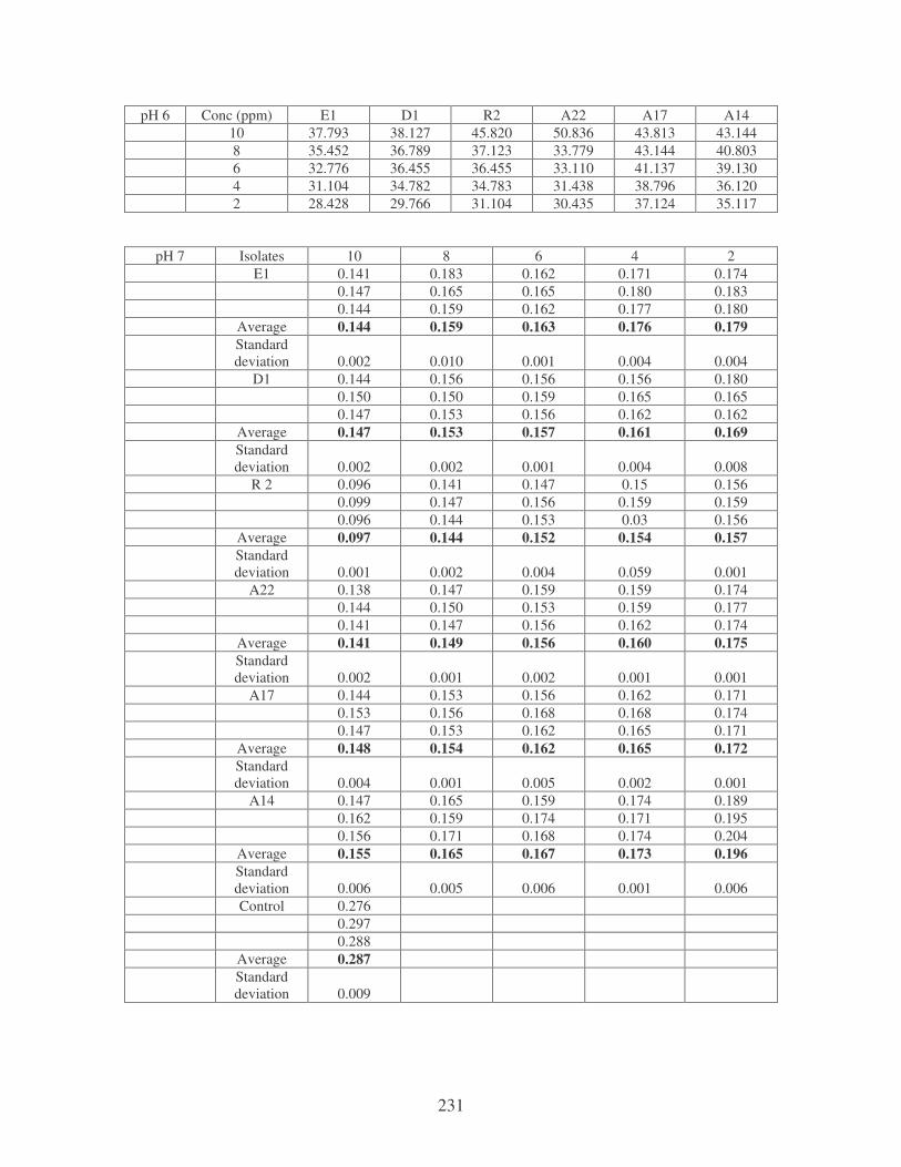
231
pH 6 Conc (ppm) E1 D1 R2 A22 A17 A14 10 37.793 38.127 45.820 50.836 43.813 43.144 8 35.452 36.789 37.123 33.779 43.144 40.803 6 32.776 36.455 36.455 33.110 41.137 39.130 4 31.104 34.782 34.783 31.438 38.796 36.120 2 28.428 29.766 31.104 30.435 37.124 35.117
pH 7 Isolates 10 8 6 4 2 E1 0.141 0.183 0.162 0.171 0.174 0.147 0.165 0.165 0.180 0.183 0.144 0.159 0.162 0.177 0.180 Average 0.144 0.159 0.163 0.176 0.179 Standard
deviation 0.002 0.010 0.001 0.004 0.004 D1 0.144 0.156 0.156 0.156 0.180 0.150 0.150 0.159 0.165 0.165 0.147 0.153 0.156 0.162 0.162 Average 0.147 0.153 0.157 0.161 0.169 Standard
deviation 0.002 0.002 0.001 0.004 0.008 R 2 0.096 0.141 0.147 0.15 0.156 0.099 0.147 0.156 0.159 0.159 0.096 0.144 0.153 0.03 0.156 Average 0.097 0.144 0.152 0.154 0.157 Standard
deviation 0.001 0.002 0.004 0.059 0.001 A22 0.138 0.147 0.159 0.159 0.174 0.144 0.150 0.153 0.159 0.177 0.141 0.147 0.156 0.162 0.174 Average 0.141 0.149 0.156 0.160 0.175 Standard
deviation 0.002 0.001 0.002 0.001 0.001 A17 0.144 0.153 0.156 0.162 0.171 0.153 0.156 0.168 0.168 0.174 0.147 0.153 0.162 0.165 0.171 Average 0.148 0.154 0.162 0.165 0.172 Standard
deviation 0.004 0.001 0.005 0.002 0.001 A14 0.147 0.165 0.159 0.174 0.189 0.162 0.159 0.174 0.171 0.195 0.156 0.171 0.168 0.174 0.204 Average 0.155 0.165 0.167 0.173 0.196 Standard
deviation 0.006 0.005 0.006 0.001 0.006 Control 0.276 0.297 0.288 Average 0.287 Standard
deviation 0.009
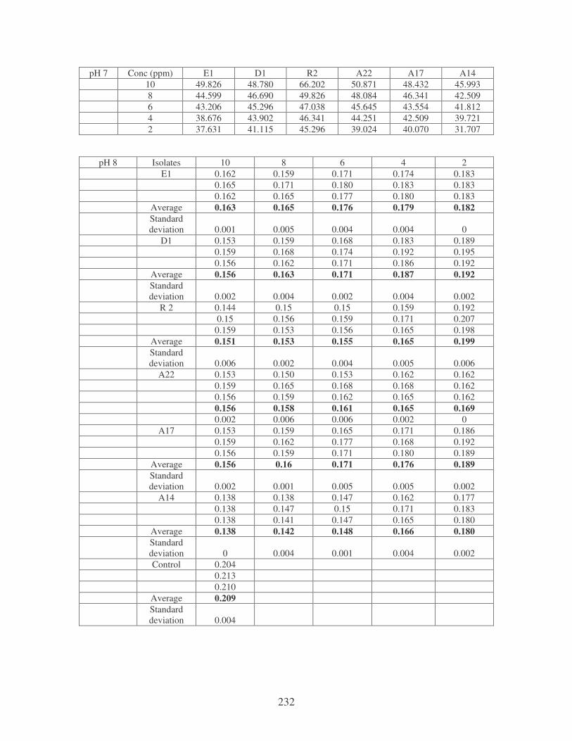
232
pH 7 Conc (ppm) E1 D1 R2 A22 A17 A14 10 49.826 48.780 66.202 50.871 48.432 45.993 8 44.599 46.690 49.826 48.084 46.341 42.509 6 43.206 45.296 47.038 45.645 43.554 41.812 4 38.676 43.902 46.341 44.251 42.509 39.721 2 37.631 41.115 45.296 39.024 40.070 31.707
pH 8 Isolates 10 8 6 4 2 E1 0.162 0.159 0.171 0.174 0.183 0.165 0.171 0.180 0.183 0.183 0.162 0.165 0.177 0.180 0.183 Average 0.163 0.165 0.176 0.179 0.182 Standard
deviation 0.001 0.005 0.004 0.004 0 D1 0.153 0.159 0.168 0.183 0.189 0.159 0.168 0.174 0.192 0.195 0.156 0.162 0.171 0.186 0.192 Average 0.156 0.163 0.171 0.187 0.192 Standard
deviation 0.002 0.004 0.002 0.004 0.002 R 2 0.144 0.15 0.15 0.159 0.192 0.15 0.156 0.159 0.171 0.207 0.159 0.153 0.156 0.165 0.198 Average 0.151 0.153 0.155 0.165 0.199 Standard
deviation 0.006 0.002 0.004 0.005 0.006 A22 0.153 0.150 0.153 0.162 0.162 0.159 0.165 0.168 0.168 0.162 0.156 0.159 0.162 0.165 0.162 0.156 0.158 0.161 0.165 0.169 0.002 0.006 0.006 0.002 0 A17 0.153 0.159 0.165 0.171 0.186 0.159 0.162 0.177 0.168 0.192 0.156 0.159 0.171 0.180 0.189 Average 0.156 0.16 0.171 0.176 0.189 Standard
deviation 0.002 0.001 0.005 0.005 0.002 A14 0.138 0.138 0.147 0.162 0.177 0.138 0.147 0.15 0.171 0.183 0.138 0.141 0.147 0.165 0.180 Average 0.138 0.142 0.148 0.166 0.180 Standard
deviation 0 0.004 0.001 0.004 0.002 Control 0.204 0.213 0.210 Average 0.209 Standard
deviation 0.004

233
pH 8 Conc (ppm) E1 D1 R2 A22 A17 A14 10 22.010 25.359 27.751 25.359 25.359 33.971 8 21.053 22.010 26.794 24.402 23.445 32.057 6 15.789 18.182 25.837 22.967 18.182 29.187 4 14.354 10.526 21.053 21.053 15.789 20.574 2 12.919 8.134 4.785 19.139 9.569 13.876
pH 9 Isolates 10 8 6 4 2
E1 0.18 0.168 0.165 0.174 0.177 0.159 0.177 0.183 0.180 0.186 0.168 0.171 0.174 0.177 0.183 Average 0.169 0.172 0.174 0.177 0.182 Standard
deviation 0.009 0.004 0.007 0.002 0.004 D1 0.147 0.165 0.168 0.174 0.183 0.150 0.174 0.174 0.186 0.186 0.147 0.168 0.171 0.18 0.183 Average 0.148 0.169 0.171 0.18 0.184 Standard
deviation 0.001 0.004 0.002 0.005 0.001 R 2 0.129 0.138 0.144 0.153 0.156 0.132 0.141 0.147 0.162 0.162 0.129 0.138 0.144 0.156 0.159 Average 0.13 0.139 0.145 0.157 0.159 Standard
deviation 0.001 0.001 0.001 0.004 0.002 A22 0.135 0.153 0.174 0.183 0.195 0.153 0.168 0.177 0.195 0.195 0.144 0.162 0.174 0.189 0.201 Average 0.144 0.161 0.175 0.188 0.197 Standard
deviation 0.007 0.006 0.001 0.005 0.003 A17 0.135 0.138 0.144 0.147 0.168 0.135 0.144 0.15 0.156 0.165 0.135 0.141 0.147 0.153 0.168 Average 0.136 0.141 0.147 0.152 0.167 Standard
deviation 0 0.002 0.002 0.004 0.001 A14 0.147 0.147 0.156 0.162 0.174 0.147 0.156 0.162 0.168 0.186 0.153 0.153 0.159 0.165 0.180 Average 0.149 0.152 0.159 0.165 0.180 Standard
deviation 0.003 0.004 0.002 0.002 0.005 Control 0.273 0.276 0.273 Average 0.274 Standard
deviation 0.001

234
pH 9 Conc (ppm) E1 D1 R2 A22 A17 A14 10 38.321 45.985 52.555 47.445 50.365 45.620 8 37.226 38.321 49.270 41.241 48.540 44.526 6 36.496 37.591 47.080 36.496 46.351 41.971 4 35.401 34.307 42.701 31.387 44.526 39.781 2 33.577 32.847 41.971 28.102 39.051 34.307
pH 10 Isolates 10 8 6 4 2
E1 0.027 0.03 0.045 0.039 0.042 0.021 0.027 0.039 0.042 0.051 0.024 0.030 0.030 0.039 0.042 Average 0.024 0.029 0.038 0.040 0.046 Standard
deviation 0.002 0.001 0.006 0.001 0.004 D1 0.027 0.054 0.054 0.063 0.075 0.036 0.063 0.072 0.072 0.081 0.030 0.060 0.069 0.069 0.087 Average 0.031 0.059 0.065 0.068 0.081 Standard
deviation 0.004 0.004 0.008 0.004 0.005 R 2 0.003 0.021 0.024 0.048 0.051 0 0.021 0.027 0.051 0.066 0.003 0.015 0.021 0.048 0.060 Average 0.002 0.019 0.024 0.049 0.059 Standard
deviation 0.001 0.003 0.002 0.001 0.006 A22 0.012 0.012 0.024 0.048 0.054 0.018 0.027 0.027 0.051 0.063 0.015 0.018 0.021 0.048 0.060 Average 0.015 0.019 0.024 0.049 0.059 Standard
deviation 0.002 0.006 0.002 0.001 0.004 A17 0.012 0.024 0.036 0.051 0.075 0.015 0.024 0.048 0.063 0.081 0.012 0.021 0.042 0.066 0.078 Average 0.013 0.023 0.042 0.06 0.078 Standard
deviation 0.001 0.001 0.005 0.006 0.002 A14 0.006 0.021 0.030 0.036 0.045 0.006 0.027 0.033 0.039 0.054 0.009 0.024 0.030 0.042 0.051 Average 0.007 0.024 0.031 0.039 0.049 Standard
deviation 0.001 0.002 0.001 0.002 0.004 Control 0.246 0.257 0.258 Average 0.258 Standard
deviation 0.005
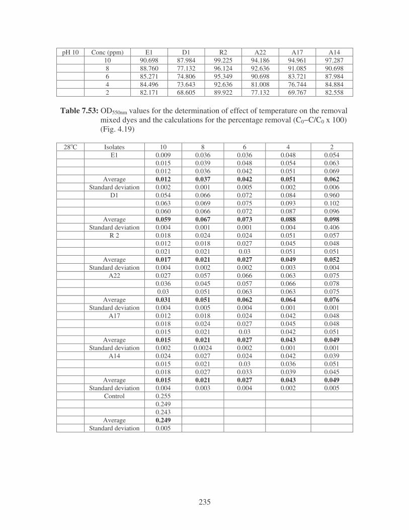
235
pH 10 Conc (ppm) E1 D1 R2 A22 A17 A14 10 90.698 87.984 99.225 94.186 94.961 97.287 8 88.760 77.132 96.124 92.636 91.085 90.698 6 85.271 74.806 95.349 90.698 83.721 87.984 4 84.496 73.643 92.636 81.008 76.744 84.884 2 82.171 68.605 89.922 77.132 69.767 82.558
Table 7.53: OD550nm values for the determination of effect of temperature on the removal mixed dyes and the calculations for the percentage removal (C0−C/C0 x 100) (Fig. 4.19)
28oC Isolates 10 8 6 4 2 E1 0.009 0.036 0.036 0.048 0.054 0.015 0.039 0.048 0.054 0.063 0.012 0.036 0.042 0.051 0.069 Average 0.012 0.037 0.042 0.051 0.062 Standard deviation 0.002 0.001 0.005 0.002 0.006 D1 0.054 0.066 0.072 0.084 0.960 0.063 0.069 0.075 0.093 0.102 0.060 0.066 0.072 0.087 0.096 Average 0.059 0.067 0.073 0.088 0.098 Standard deviation 0.004 0.001 0.001 0.004 0.406 R 2 0.018 0.024 0.024 0.051 0.057 0.012 0.018 0.027 0.045 0.048 0.021 0.021 0.03 0.051 0.051 Average 0.017 0.021 0.027 0.049 0.052 Standard deviation 0.004 0.002 0.002 0.003 0.004 A22 0.027 0.057 0.066 0.063 0.075 0.036 0.045 0.057 0.066 0.078 0.03 0.051 0.063 0.063 0.075 Average 0.031 0.051 0.062 0.064 0.076 Standard deviation 0.004 0.005 0.004 0.001 0.001 A17 0.012 0.018 0.024 0.042 0.048 0.018 0.024 0.027 0.045 0.048 0.015 0.021 0.03 0.042 0.051 Average 0.015 0.021 0.027 0.043 0.049 Standard deviation 0.002 0.0024 0.002 0.001 0.001 A14 0.024 0.027 0.024 0.042 0.039 0.015 0.021 0.03 0.036 0.051 0.018 0.027 0.033 0.039 0.045 Average 0.015 0.021 0.027 0.043 0.049 Standard deviation 0.004 0.003 0.004 0.002 0.005 Control 0.255 0.249 0.243 Average 0.249 Standard deviation 0.005
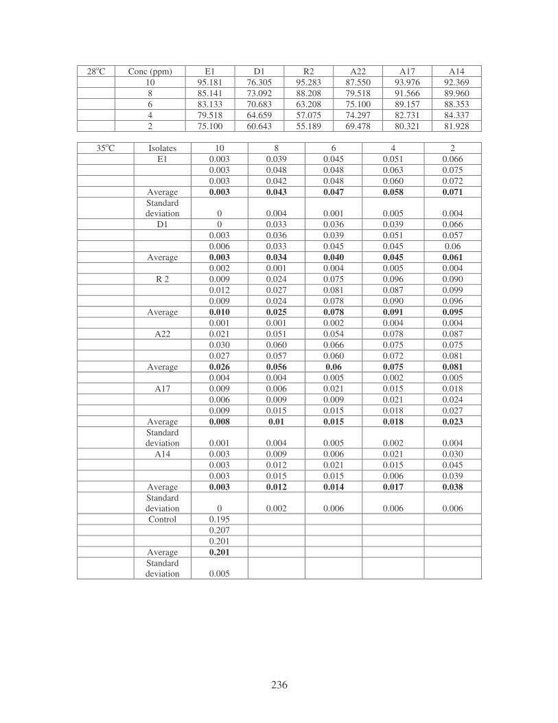
236
28oC Conc (ppm) E1 D1 R2 A22 A17 A14 10 95.181 76.305 95.283 87.550 93.976 92.369 8 85.141 73.092 88.208 79.518 91.566 89.960 6 83.133 70.683 63.208 75.100 89.157 88.353 4 79.518 64.659 57.075 74.297 82.731 84.337 2 75.100 60.643 55.189 69.478 80.321 81.928
35oC Isolates 10 8 6 4 2
E1 0.003 0.039 0.045 0.051 0.066 0.003 0.048 0.048 0.063 0.075 0.003 0.042 0.048 0.060 0.072 Average 0.003 0.043 0.047 0.058 0.071 Standard
deviation 0 0.004 0.001 0.005 0.004 D1 0 0.033 0.036 0.039 0.066 0.003 0.036 0.039 0.051 0.057 0.006 0.033 0.045 0.045 0.06 Average 0.003 0.034 0.040 0.045 0.061 0.002 0.001 0.004 0.005 0.004 R 2 0.009 0.024 0.075 0.096 0.090 0.012 0.027 0.081 0.087 0.099 0.009 0.024 0.078 0.090 0.096 Average 0.010 0.025 0.078 0.091 0.095 0.001 0.001 0.002 0.004 0.004 A22 0.021 0.051 0.054 0.078 0.087 0.030 0.060 0.066 0.075 0.075 0.027 0.057 0.060 0.072 0.081 Average 0.026 0.056 0.06 0.075 0.081 0.004 0.004 0.005 0.002 0.005 A17 0.009 0.006 0.021 0.015 0.018 0.006 0.009 0.009 0.021 0.024 0.009 0.015 0.015 0.018 0.027 Average 0.008 0.01 0.015 0.018 0.023 Standard
deviation 0.001 0.004 0.005 0.002 0.004 A14 0.003 0.009 0.006 0.021 0.030 0.003 0.012 0.021 0.015 0.045 0.003 0.015 0.015 0.006 0.039 Average 0.003 0.012 0.014 0.017 0.038 Standard
deviation 0 0.002 0.006 0.006 0.006 Control 0.195 0.207 0.201 Average 0.201 Standard
deviation 0.005

237
35oC Conc (ppm) E1 D1 R2 A22 A17 A14 10 98.507 98.507 84.080 87.736 96.020 98.507 8 78.607 83.085 80.597 73.585 95.025 94.030 6 76.617 80.100 74.627 71.698 92.537 93.035 4 71.144 77.612 69.652 64.623 91.045 91.542 2 64.677 69.652 63.184 61.792 88.557 81.095
40oC Isolates 10 8 6 4 2
E1 0.003 0.012 0.015 0.018 0.036 0.006 0.006 0.027 0.027 0.048 0.003 0.009 0.018 0.024 0.042 Average 0.004 0.009 0.02 0.023 0.041 Standard
deviation 0.001 0.002 0.005 0.004 0.005 D1 0.006 0.009 0.009 0.018 0.030 0.009 0.015 0.021 0.036 0.033 0.006 0.012 0.015 0.027 0.030 Average 0.007 0.012 0.015 0.027 0.031 Standard
deviation 0.001 0.002 0.005 0.007 0.001 R 2 0 0.003 0.006 0.027 0.030 0 0.012 0.006 0.018 0.045 0.003 0.006 0.015 0.024 0.036 Average 0.001 0.007 0.009 0.023 0.037 Standard
deviation 0.001 0.004 0.004 0.004 0.006 A22 0.015 0.027 0.03 0.024 0.036 0.024 0.018 0.021 0.039 0.039 0.018 0.021 0.024 0.033 0.042 Average 0.019 0.022 0.025 0.032 0.039 Standard
deviation 0.004 0.004 0.004 0.006 0.002 A17 0 0.006 0.006 0.006 0.015 0 0.003 0.009 0.012 0.015 0.003 0.006 0.006 0.009 0.021 Average 0.001 0.005 0.007 0.009 0.017 Standard
deviation 0.001 0.001 0.001 0.002 0.003 A14 0.003 0.003 0.006 0.009 0.009 0.003 0.006 0.009 0.012 0.015 0.006 0.009 0.009 0.009 0.021 Average 0.004 0.006 0.008 0.01 0.015 Standard
deviation 0.001 0.002 0.001 0.001 0.005 Control 0.204 0.207 0.204 Average 0.205 Standard
deviation 0.001

238
40oC Conc (ppm) E1 D1 R2 A22 A17 A14 10 98.049 96.585 99.512 90.732 99.512 98.049 8 93.780 94.146 96.585 89.268 97.561 97.073 6 90.244 92.683 95.610 87.805 96.585 96.098 4 88.780 86.829 88.780 84.390 95.610 95.123 2 80.000 84.878 81.951 80.976 91.707 92.683
45oC Isolates 10 8 6 4 2
E1 0.006 0.018 0.009 0.030 0.033 0.012 0.009 0.018 0.021 0.024 0.009 0.012 0.027 0.024 0.027 Average 0.090 0.013 0.018 0.025 0.028 Standard
deviation 0.002 0.004 0.007 0.004 0.004 D1 0.012 0.009 0.018 0.045 0.048 0.009 0.015 0.024 0.033 0.063 0.015 0.021 0.027 0.039 0.057 Average 0.012 0.015 0.023 0.039 0.056 Standard
deviation 0.002 0.005 0.004 0.005 0.006 R 2 0.027 0.033 0.045 0.057 0.066 0.036 0.045 0.057 0.066 0.081 0.033 0.039 0.051 0.06 0.075 Average 0.032 0.039 0.051 0.061 0.074 Standard
deviation 0.004 0.005 0.005 0.004 0.006 A22 0.051 0.048 0.051 0.054 0.075 0.054 0.054 0.063 0.069 0.078 0.051 0.060 0.057 0.063 0.075 Average 0.052 0.054 0.056 0.062 0.076 Standard
deviation 0.001 0.005 0.005 0.006 0.001 A17 0.048 0.072 0.078 0.081 0.084 0.072 0.087 0.090 0.096 0.099 0.066 0.081 0.084 0.090 0.093 Average 0.062 0.080 0.084 0.089 0.092 Standard
deviation 0.010 0.006 0.005 0.006 0.006 A14 0.018 0.033 0.042 0.042 0.039 0.021 0.045 0.051 0.054 0.057 0.018 0.039 0.045 0.048 0.054 Average 0.019 0.039 0.046 0.048 0.05 Standard
deviation 0.001 0.005 0.004 0.005 0.008 Control 0.201 0.219 0.216 Average 0.212 Standard
deviation 0.008
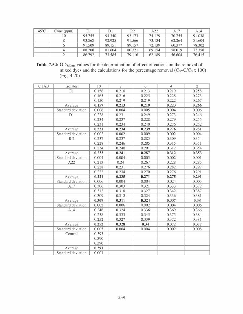
239
45oC Conc (ppm) E1 D1 R2 A22 A17 A14 10 95.755 94.340 93.173 74.129 70.755 91.038 8 93.868 92.925 91.566 73.134 62.264 81.604 6 91.509 89.151 89.157 72.139 60.377 78.302 4 88.208 81.604 80.321 69.154 58.019 77.358 2 86.792 73.585 79.116 62.189 56.604 76.415
Table 7.54: OD550nm values for the determination of effect of cations on the removal of mixed dyes and the calculations for the percentage removal (C0−C/C0 x 100) (Fig. 4.20)
CTAB Isolates 10 8 6 4 2 E1 0.156 0.210 0.213 0.219 0.258 0.165 0.216 0.225 0.228 0.273 0.150 0.219 0.219 0.222 0.267 Average 0.157 0.213 0.219 0.223 0.266 Standard deviation 0.006 0.004 0.005 0.004 0.006 D1 0.228 0.231 0.249 0.273 0.246 0.234 0.237 0.228 0.279 0.255 0.231 0.234 0.240 0.276 0.252 Average 0.231 0.234 0.239 0.276 0.251 Standard deviation 0.002 0.002 0.009 0.002 0.004 R 2 0.237 0.237 0.285 0.309 0.354 0.228 0.246 0.285 0.315 0.351 0.234 0.240 0.291 0.312 0.354 Average 0.233 0.241 0.287 0.312 0.353 Standard deviation 0.004 0.004 0.003 0.002 0.001 A22 0.213 0.24 0.267 0.228 0.285 0.228 0.231 0.276 0.282 0.297 0.222 0.234 0.270 0.276 0.291 Average 0.221 0.235 0.271 0.275 0.291 Standard deviation 0.006 0.004 0.004 0.024 0.005 A17 0.306 0.303 0.321 0.333 0.372 0.312 0.318 0.327 0.342 0.387 0.309 0.312 0.324 0.336 0.381 Average 0.309 0.311 0.324 0.337 0.38 Standard deviation 0.002 0.006 0.002 0.004 0.006 A14 0.246 0.324 0.336 0.369 0.366 0.258 0.333 0.345 0.375 0.384 0.252 0.327 0.339 0.372 0.381 Average 0.252 0.328 0.34 0.372 0.377 Standard deviation 0.005 0.004 0.004 0.002 0.008 Control 0.393 0.390 0.390 Average 0.391 Standard deviation 0.001

240
CTAB Conc (ppm) E1 D1 R2 A22 A17 A14 10 59.847 40.921 40.409 43.478 20.972 35.294 8 45.424 40.153 38.636 39.898 20.460 16.113 6 43.990 38.875 26.598 30.691 17.136 13.043 4 42.967 29.412 20.205 29.668 13.811 4.859 2 31.969 10.230 9.719 25.575 2.831 3.581
CaCl2 Isolates 10 8 6 4 2 E1 0.039 0.042 0.045 0.051 0.063 0.051 0.057 0.06 0.069 0.066 0.045 0.048 0.054 0.060 0.063 Average 0.045 0.490 0.053 0.060 0.064 Standard
deviation 0.005 0.006 0.006 0.007 0.001 D1 0.072 0.078 0.087 0.090 0.093 0.075 0.078 0.093 0.096 0.105 0.072 0.084 0.090 0.093 0.099 Average 0.073 0.08 0.09 0.093 0.099 Standard
deviation 0.001 0.003 0.002 0.002 0.005 R 2 0.048 0.051 0.045 0.069 0.060 0.054 0.060 0.075 0.06 0.075 0.051 0.057 0.066 0.063 0.066 Average 0.051 0.056 0.062 0.064 0.067 Standard
deviation 0.002 0.004 0.013 0.004 0.006 A22 0.075 0.075 0.075 0.081 0.102 0.078 0.069 0.087 0.087 0.099 0.075 0.078 0.081 0.084 0.096 Average 0.075 0.079 0.081 0.084 0.097 Standard
deviation 0.001 0.004 0.005 0.002 0.002 A17 0.042 0.054 0.072 0.069 0.075 0.048 0.066 0.06 0.075 0.081 0.045 0.060 0.066 0.072 0.078 Average 0.045 0.06 0.066 0.072 0.078 Standard
deviation 0.002 0.005 0.006 0.002 0.002 A14 0.027 0.039 0.042 0.054 0.066 0.039 0.045 0.051 0.057 0.075 0.033 0.042 0.045 0.054 0.072 Average 0.033 0.042 0.046 0.055 0.071 Standard
deviation 0.005 0.002 0.004 0.001 0.004 Control 0.198 0.219 0.210 Average 0.209 Standard
deviation 0.009
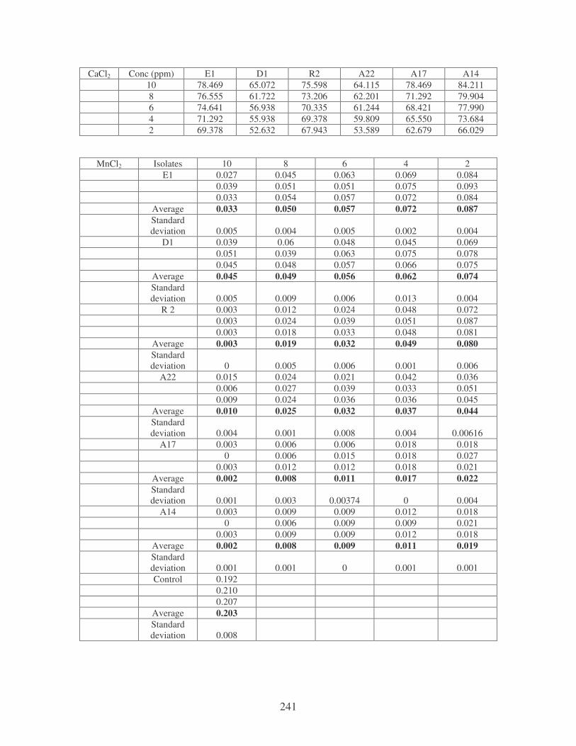
241
CaCl2 Conc (ppm) E1 D1 R2 A22 A17 A14 10 78.469 65.072 75.598 64.115 78.469 84.211 8 76.555 61.722 73.206 62.201 71.292 79.904 6 74.641 56.938 70.335 61.244 68.421 77.990 4 71.292 55.938 69.378 59.809 65.550 73.684 2 69.378 52.632 67.943 53.589 62.679 66.029
MnCl2 Isolates 10 8 6 4 2 E1 0.027 0.045 0.063 0.069 0.084 0.039 0.051 0.051 0.075 0.093 0.033 0.054 0.057 0.072 0.084 Average 0.033 0.050 0.057 0.072 0.087 Standard
deviation 0.005 0.004 0.005 0.002 0.004 D1 0.039 0.06 0.048 0.045 0.069 0.051 0.039 0.063 0.075 0.078 0.045 0.048 0.057 0.066 0.075 Average 0.045 0.049 0.056 0.062 0.074 Standard
deviation 0.005 0.009 0.006 0.013 0.004 R 2 0.003 0.012 0.024 0.048 0.072 0.003 0.024 0.039 0.051 0.087 0.003 0.018 0.033 0.048 0.081 Average 0.003 0.019 0.032 0.049 0.080 Standard
deviation 0 0.005 0.006 0.001 0.006 A22 0.015 0.024 0.021 0.042 0.036 0.006 0.027 0.039 0.033 0.051 0.009 0.024 0.036 0.036 0.045 Average 0.010 0.025 0.032 0.037 0.044 Standard
deviation 0.004 0.001 0.008 0.004 0.00616 A17 0.003 0.006 0.006 0.018 0.018 0 0.006 0.015 0.018 0.027 0.003 0.012 0.012 0.018 0.021 Average 0.002 0.008 0.011 0.017 0.022 Standard
deviation 0.001 0.003 0.00374 0 0.004 A14 0.003 0.009 0.009 0.012 0.018 0 0.006 0.009 0.009 0.021 0.003 0.009 0.009 0.012 0.018 Average 0.002 0.008 0.009 0.011 0.019 Standard
deviation 0.001 0.001 0 0.001 0.001 Control 0.192 0.210 0.207 Average 0.203 Standard
deviation 0.008
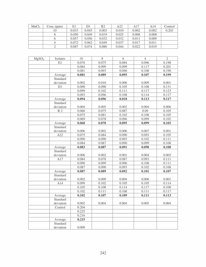
242
MnCl2 Conc (ppm) E1 D1 R2 A22 A17 A14 Control 10 0.033 0.045 0.003 0.010 0.002 0.002 0.203 8 0.050 0.049 0.019 0.025 0.008 0.008 6 0.057 0.056 0.032 0.032 0.011 0.009 4 0.072 0.062 0.049 0.037 0.017 0.011 2 0.087 0.074 0.080 0.044 0.022 0.019
MgSO4 Isolates 10 8 6 4 2 E1 0.078 0.075 0.084 0.096 0.198 0.084 0.099 0.099 0.117 0.201 0.081 0.093 0.096 0.108 0.198 Average 0.081 0.089 0.095 0.107 0.199 Standard
deviation 0.002 0.010 0.006 0.009 0.001 D1 0.090 0.090 0.105 0.108 0.131 0.099 0.102 0.111 0.117 0.123 0.093 0.096 0.108 0.114 0.117 Average 0.094 0.096 0.018 0.113 0.117 Standard
deviation 0.004 0.005 0.002 0.004 0.006 R 2 0.060 0.075 0.087 0.09 0.105 0.075 0.081 0.102 0.108 0.105 0.069 0.078 0.096 0.099 0.102 Average 0.068 0.078 0.095 0.099 0.103 Standard
deviation 0.006 0.002 0.006 0.007 0.001 A22 0.075 0.084 0.090 0.093 0.105 0.090 0.090 0.093 0.102 0.111 0.084 0.087 0.090 0.099 0.108 Average 0.083 0.087 0.091 0.098 0.108 Standard
deviation 0.006 0.002 0.001 0.004 0.002 A17 0.084 0.078 0.087 0.093 0.111 0.090 0.099 0.096 0.108 0.111 0.087 0.090 0.093 0.102 0.108 Average 0.087 0.089 0.092 0.101 0.107 Standard
deviation 0.002 0.009 0.004 0.006 0.001 A14 0.099 0.102 0.105 0.105 0.114 0.105 0.108 0.114 0.117 0.108 0.102 0.111 0.108 0.111 0.117 Average 0.102 0.107 0.109 0.111 0.113 Standard
deviation 0.002 0.004 0.004 0.005 0.004 Control 0.204 0.225 0.216 Average 0.215 Standard
deviation 0.009
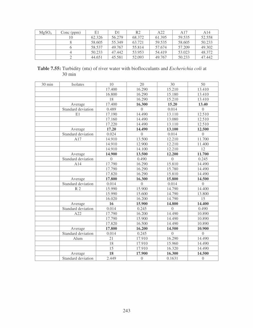
243
MgSO4 Conc (ppm) E1 D1 R2 A22 A17 A14 10 62.326 56.279 68.372 61.395 59.535 52.558 8 58.605 55.349 63.721 59.535 58.605 50.233 6 58.537 49.767 55.814 57.674 57.209 49.302 4 50.233 47.442 53.953 54.419 53.023 48.372 2 44.651 45.581 52.093 49.767 50.233 47.442
Table 7.55: Turbidity (ntu) of river water with bioflocculants and Escherichia coli at 30 min
30 min Isolates 10 20 30 50 17.400 16.290 15.210 13.410 16.800 16.290 15.180 13.410 18 16.290 15.210 13.410 Average 17.400 16.300 15.20 13.40
Standard deviation 0.489 0 0.014 0 E1 17.190 14.490 13.110 12.510 17.160 14.490 13.080 12.510 17.220 14.490 13.110 12.510 Average 17.20 14.490 13.100 12.500 Standard deviation 0.024 0 0.014 0 A17 14.910 13.500 12.210 11.700 14.910 12.900 12.210 11.400 14.910 14.100 12.210 12 Average 14.900 13.500 12.200 11.700 Standard deviation 0 0.490 0 0.245 A14 17.790 16.290 15.810 14.490 17.790 16.290 15.780 14.490 17.820 16.290 15.810 14.490 Average 17.800 16.300 15.800 14.500 Standard deviation 0.014 0 0.014 0 R 2 15.990 15.900 14.790 14.400 15.990 15.600 14.790 13.800 16.020 16.200 14.790 15 Average 16 15.900 14.800 14.400 Standard deviation 0.014 0.245 0 0.490 A22 17.790 16.200 14.490 10.890 17.790 15.900 14.490 10.890 17.820 16.500 14.490 10.890 Average 17.800 16.200 14.500 10.900 Standard deviation 0.014 0.245 0 0 Alum 21 17.910 16.290 14.490 18 17.910 15.960 14.490 15 17.910 16.320 14.490 Average 18 17.900 16.300 14.500 Standard deviation 2.449 0 0.1631 0
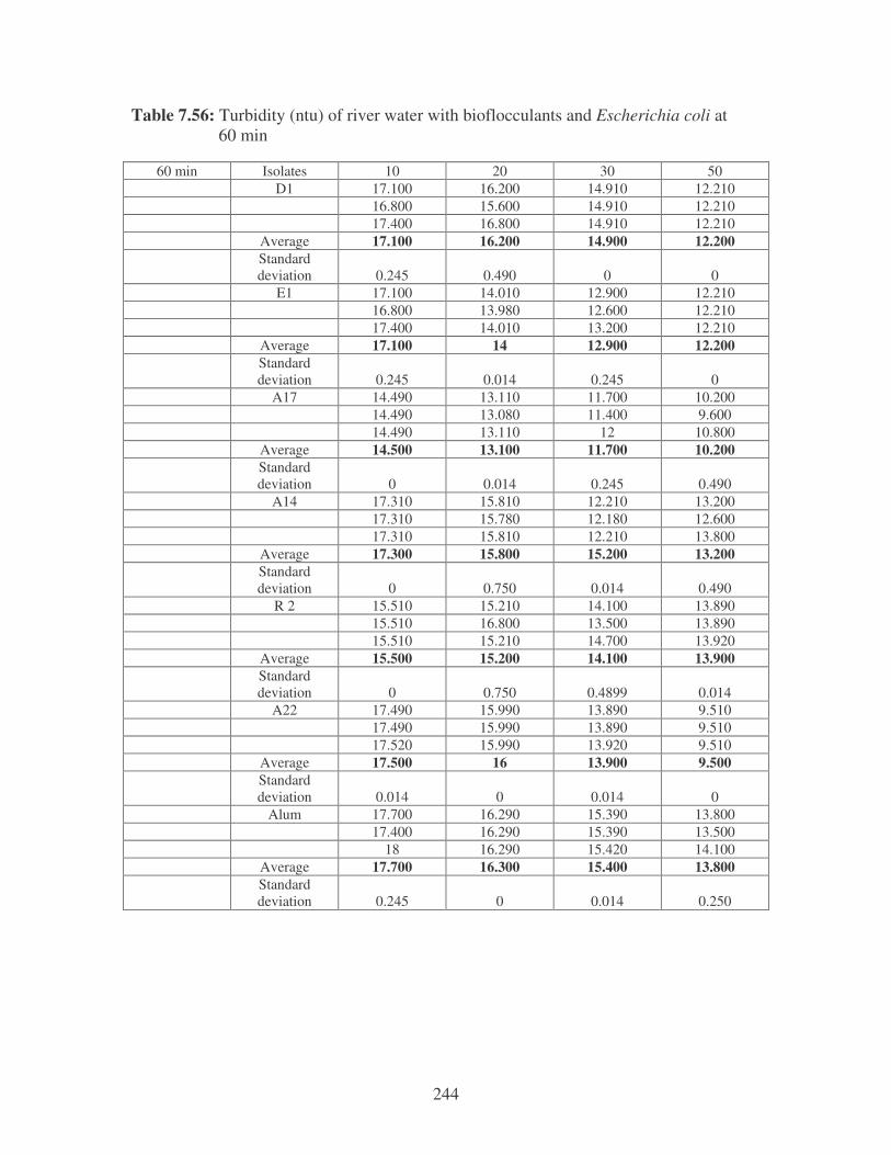
244
Table 7.56: Turbidity (ntu) of river water with bioflocculants and Escherichia coli at 60 min
60 min Isolates 10 20 30 50 D1 17.100 16.200 14.910 12.210 16.800 15.600 14.910 12.210 17.400 16.800 14.910 12.210 Average 17.100 16.200 14.900 12.200 Standard
deviation 0.245 0.490 0 0 E1 17.100 14.010 12.900 12.210 16.800 13.980 12.600 12.210 17.400 14.010 13.200 12.210 Average 17.100 14 12.900 12.200 Standard
deviation 0.245 0.014 0.245 0 A17 14.490 13.110 11.700 10.200 14.490 13.080 11.400 9.600 14.490 13.110 12 10.800 Average 14.500 13.100 11.700 10.200 Standard
deviation 0 0.014 0.245 0.490 A14 17.310 15.810 12.210 13.200 17.310 15.780 12.180 12.600 17.310 15.810 12.210 13.800 Average 17.300 15.800 15.200 13.200 Standard
deviation 0 0.750 0.014 0.490 R 2 15.510 15.210 14.100 13.890 15.510 16.800 13.500 13.890 15.510 15.210 14.700 13.920 Average 15.500 15.200 14.100 13.900 Standard
deviation 0 0.750 0.4899 0.014 A22 17.490 15.990 13.890 9.510 17.490 15.990 13.890 9.510 17.520 15.990 13.920 9.510 Average 17.500 16 13.900 9.500 Standard
deviation 0.014 0 0.014 0 Alum 17.700 16.290 15.390 13.800 17.400 16.290 15.390 13.500 18 16.290 15.420 14.100 Average 17.700 16.300 15.400 13.800 Standard
deviation 0.245 0 0.014 0.250
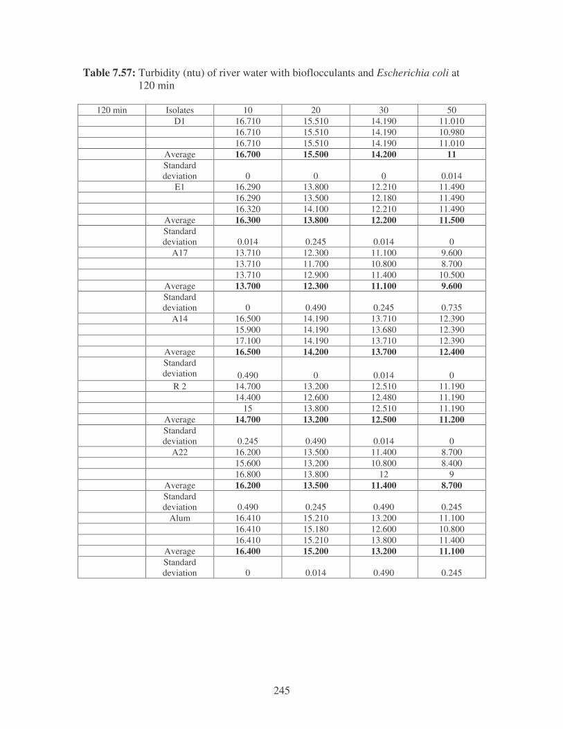
245
Table 7.57: Turbidity (ntu) of river water with bioflocculants and Escherichia coli at 120 min
120 min Isolates 10 20 30 50 D1 16.710 15.510 14.190 11.010 16.710 15.510 14.190 10.980 16.710 15.510 14.190 11.010 Average 16.700 15.500 14.200 11 Standard
deviation 0 0 0 0.014 E1 16.290 13.800 12.210 11.490 16.290 13.500 12.180 11.490 16.320 14.100 12.210 11.490 Average 16.300 13.800 12.200 11.500 Standard
deviation 0.014 0.245 0.014 0 A17 13.710 12.300 11.100 9.600 13.710 11.700 10.800 8.700 13.710 12.900 11.400 10.500 Average 13.700 12.300 11.100 9.600 Standard
deviation 0 0.490 0.245 0.735 A14 16.500 14.190 13.710 12.390 15.900 14.190 13.680 12.390 17.100 14.190 13.710 12.390 Average 16.500 14.200 13.700 12.400 Standard
deviation 0.490 0 0.014 0 R 2 14.700 13.200 12.510 11.190 14.400 12.600 12.480 11.190 15 13.800 12.510 11.190 Average 14.700 13.200 12.500 11.200 Standard
deviation 0.245 0.490 0.014 0 A22 16.200 13.500 11.400 8.700 15.600 13.200 10.800 8.400 16.800 13.800 12 9 Average 16.200 13.500 11.400 8.700 Standard
deviation 0.490 0.245 0.490 0.245 Alum 16.410 15.210 13.200 11.100 16.410 15.180 12.600 10.800 16.410 15.210 13.800 11.400 Average 16.400 15.200 13.200 11.100 Standard
deviation 0 0.014 0.490 0.245
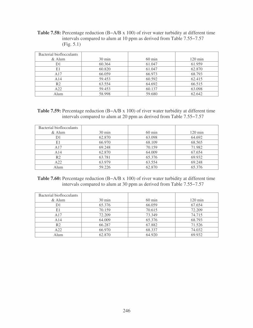
246
Table 7.58: Percentage reduction (B−A/B x 100) of river water turbidity at different time intervals compared to alum at 10 ppm as derived from Table 7.55−7.57 (Fig. 5.1) Bacterial bioflocculants
& Alum 30 min 60 min 120 min D1 60.364 61.047 61.959 E1 60.820 61.047 62.870
A17 66.059 66.973 68.793 A14 59.453 60.592 62.415 R2 63.554 64.692 66.515
A22 59.453 60.137 63.098 Alum 58.998 59.680 62.642
Table 7.59: Percentage reduction (B−A/B x 100) of river water turbidity at different time intervals compared to alum at 20 ppm as derived from Table 7.55−7.57 Bacterial bioflocculants
& Alum 30 min 60 min 120 min D1 62.870 63.098 64.692 E1 66.970 68.109 68.565
A17 69.248 70.159 71.982 A14 62.870 64.009 67.654 R2 63.781 65.376 69.932
A22 63.979 63.554 69.248 Alum 59.226 62.870 65.376
Table 7.60: Percentage reduction (B−A/B x 100) of river water turbidity at different time intervals compared to alum at 30 ppm as derived from Table 7.55−7.57 Bacterial bioflocculants
& Alum 30 min 60 min 120 min D1 65.376 66.059 67.654 E1 70.159 70.615 72.209
A17 72.209 73.349 74.715 A14 64.009 65.376 68.793 R2 66.287 67.882 71.526
A22 66.970 68.337 74.032 Alum 62.870 64.920 69.932
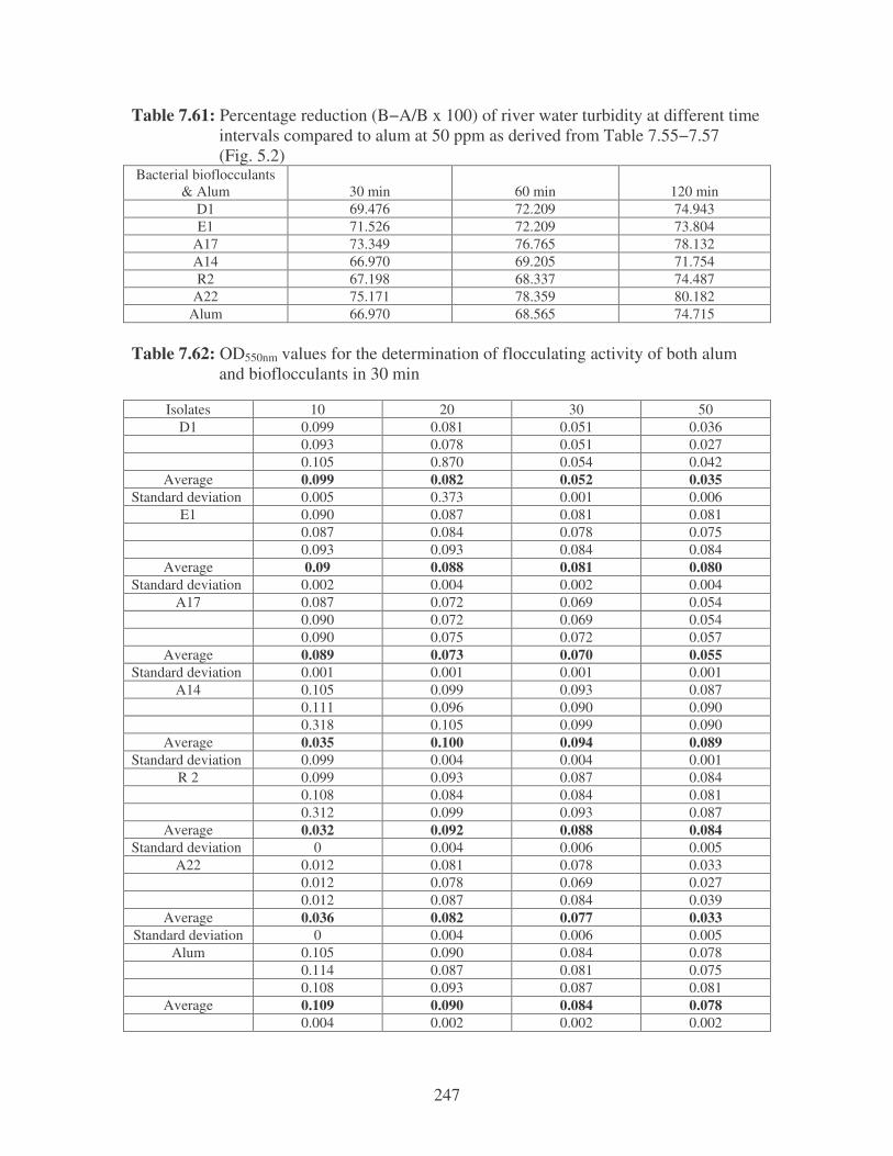
247
Table 7.61: Percentage reduction (B−A/B x 100) of river water turbidity at different time intervals compared to alum at 50 ppm as derived from Table 7.55−7.57 (Fig. 5.2) Bacterial bioflocculants
& Alum 30 min 60 min 120 min D1 69.476 72.209 74.943 E1 71.526 72.209 73.804
A17 73.349 76.765 78.132 A14 66.970 69.205 71.754 R2 67.198 68.337 74.487
A22 75.171 78.359 80.182 Alum 66.970 68.565 74.715
Table 7.62: OD550nm values for the determination of flocculating activity of both alum and bioflocculants in 30 min
Isolates 10 20 30 50 D1 0.099 0.081 0.051 0.036
0.093 0.078 0.051 0.027 0.105 0.870 0.054 0.042
Average 0.099 0.082 0.052 0.035 Standard deviation 0.005 0.373 0.001 0.006
E1 0.090 0.087 0.081 0.081 0.087 0.084 0.078 0.075 0.093 0.093 0.084 0.084
Average 0.09 0.088 0.081 0.080 Standard deviation 0.002 0.004 0.002 0.004
A17 0.087 0.072 0.069 0.054 0.090 0.072 0.069 0.054 0.090 0.075 0.072 0.057
Average 0.089 0.073 0.070 0.055 Standard deviation 0.001 0.001 0.001 0.001
A14 0.105 0.099 0.093 0.087 0.111 0.096 0.090 0.090 0.318 0.105 0.099 0.090
Average 0.035 0.100 0.094 0.089 Standard deviation 0.099 0.004 0.004 0.001
R 2 0.099 0.093 0.087 0.084 0.108 0.084 0.084 0.081 0.312 0.099 0.093 0.087
Average 0.032 0.092 0.088 0.084 Standard deviation 0 0.004 0.006 0.005
A22 0.012 0.081 0.078 0.033 0.012 0.078 0.069 0.027 0.012 0.087 0.084 0.039
Average 0.036 0.082 0.077 0.033 Standard deviation 0 0.004 0.006 0.005
Alum 0.105 0.090 0.084 0.078 0.114 0.087 0.081 0.075 0.108 0.093 0.087 0.081
Average 0.109 0.090 0.084 0.078 0.004 0.002 0.002 0.002
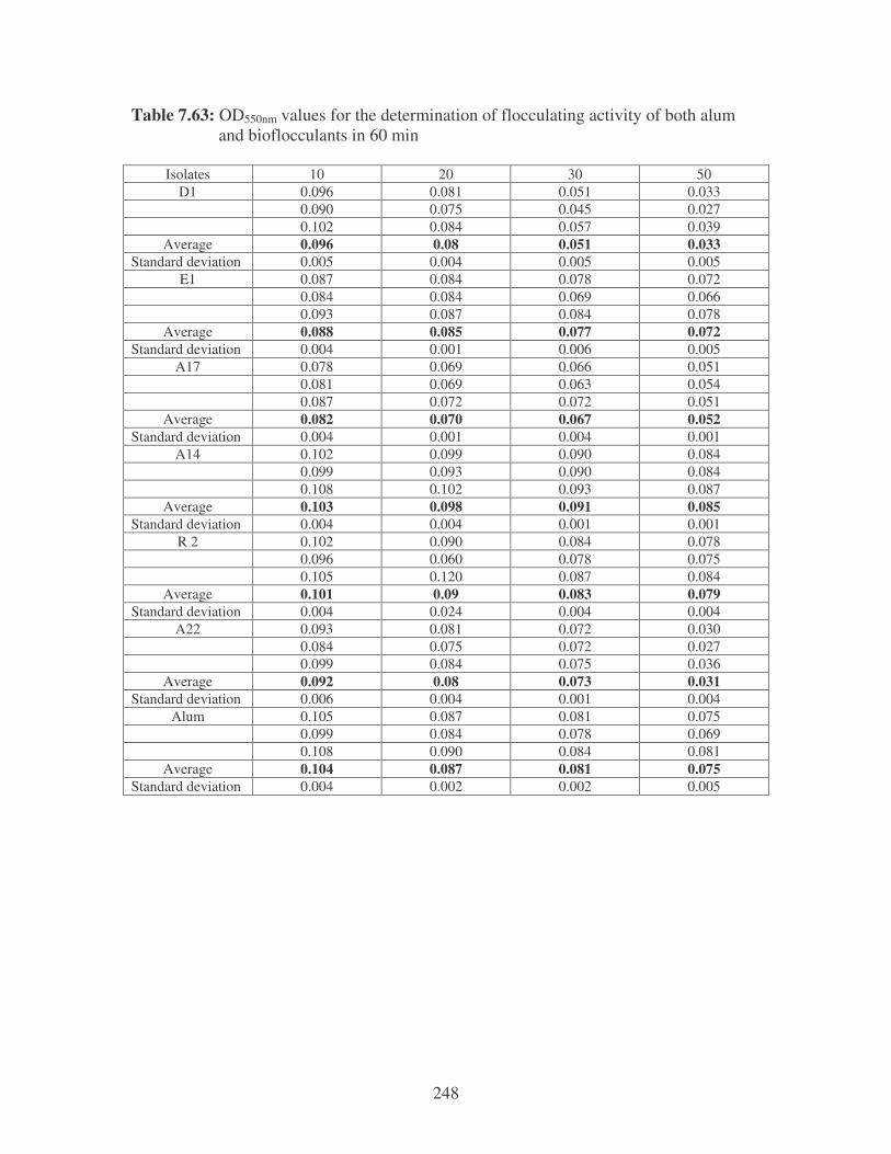
248
Table 7.63: OD550nm values for the determination of flocculating activity of both alum and bioflocculants in 60 min
Isolates 10 20 30 50 D1 0.096 0.081 0.051 0.033
0.090 0.075 0.045 0.027 0.102 0.084 0.057 0.039
Average 0.096 0.08 0.051 0.033 Standard deviation 0.005 0.004 0.005 0.005
E1 0.087 0.084 0.078 0.072 0.084 0.084 0.069 0.066 0.093 0.087 0.084 0.078
Average 0.088 0.085 0.077 0.072 Standard deviation 0.004 0.001 0.006 0.005
A17 0.078 0.069 0.066 0.051 0.081 0.069 0.063 0.054 0.087 0.072 0.072 0.051
Average 0.082 0.070 0.067 0.052 Standard deviation 0.004 0.001 0.004 0.001
A14 0.102 0.099 0.090 0.084 0.099 0.093 0.090 0.084 0.108 0.102 0.093 0.087
Average 0.103 0.098 0.091 0.085 Standard deviation 0.004 0.004 0.001 0.001
R 2 0.102 0.090 0.084 0.078 0.096 0.060 0.078 0.075 0.105 0.120 0.087 0.084
Average 0.101 0.09 0.083 0.079 Standard deviation 0.004 0.024 0.004 0.004
A22 0.093 0.081 0.072 0.030 0.084 0.075 0.072 0.027 0.099 0.084 0.075 0.036
Average 0.092 0.08 0.073 0.031 Standard deviation 0.006 0.004 0.001 0.004
Alum 0.105 0.087 0.081 0.075 0.099 0.084 0.078 0.069 0.108 0.090 0.084 0.081
Average 0.104 0.087 0.081 0.075 Standard deviation 0.004 0.002 0.002 0.005
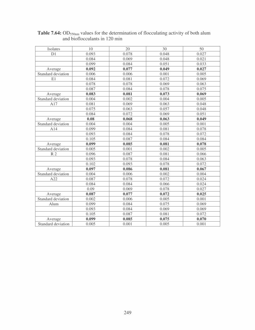
249
Table 7.64: OD550nm values for the determination of flocculating activity of both alum and bioflocculants in 120 min
Isolates 10 20 30 50 D1 0.093 0.078 0.048 0.027
0.084 0.069 0.048 0.021 0.099 0.084 0.051 0.033
Average 0.092 0.077 0.049 0.027 Standard deviation 0.006 0.006 0.001 0.005
E1 0.084 0.081 0.072 0.069 0.078 0.078 0.069 0.063 0.087 0.084 0.078 0.075
Average 0.083 0.081 0.073 0.069 Standard deviation 0.004 0.002 0.004 0.005
A17 0.081 0.069 0.063 0.048 0.075 0.063 0.057 0.048 0.084 0.072 0.069 0.051
Average 0.08 0.068 0.063 0.049 Standard deviation 0.004 0.004 0.005 0.001
A14 0.099 0.084 0.081 0.078 0.093 0.084 0.078 0.072 0.105 0.087 0.084 0.084
Average 0.099 0.085 0.081 0.078 Standard deviation 0.005 0.001 0.002 0.005
R 2 0.096 0.087 0.081 0.066 0.093 0.078 0.084 0.063 0.102 0.093 0.078 0.072
Average 0.097 0.086 0.081 0.067 Standard deviation 0.004 0.006 0.002 0.004
A22 0.087 0.078 0.072 0.024 0.084 0.084 0.066 0.024 0.09 0.069 0.078 0.027
Average 0.087 0.077 0.072 0.025 Standard deviation 0.002 0.006 0.005 0.001
Alum 0.099 0.084 0.075 0.069 0.093 0.084 0.069 0.069 0.105 0.087 0.081 0.072
Average 0.099 0.085 0.075 0.070 Standard deviation 0.005 0.001 0.005 0.001
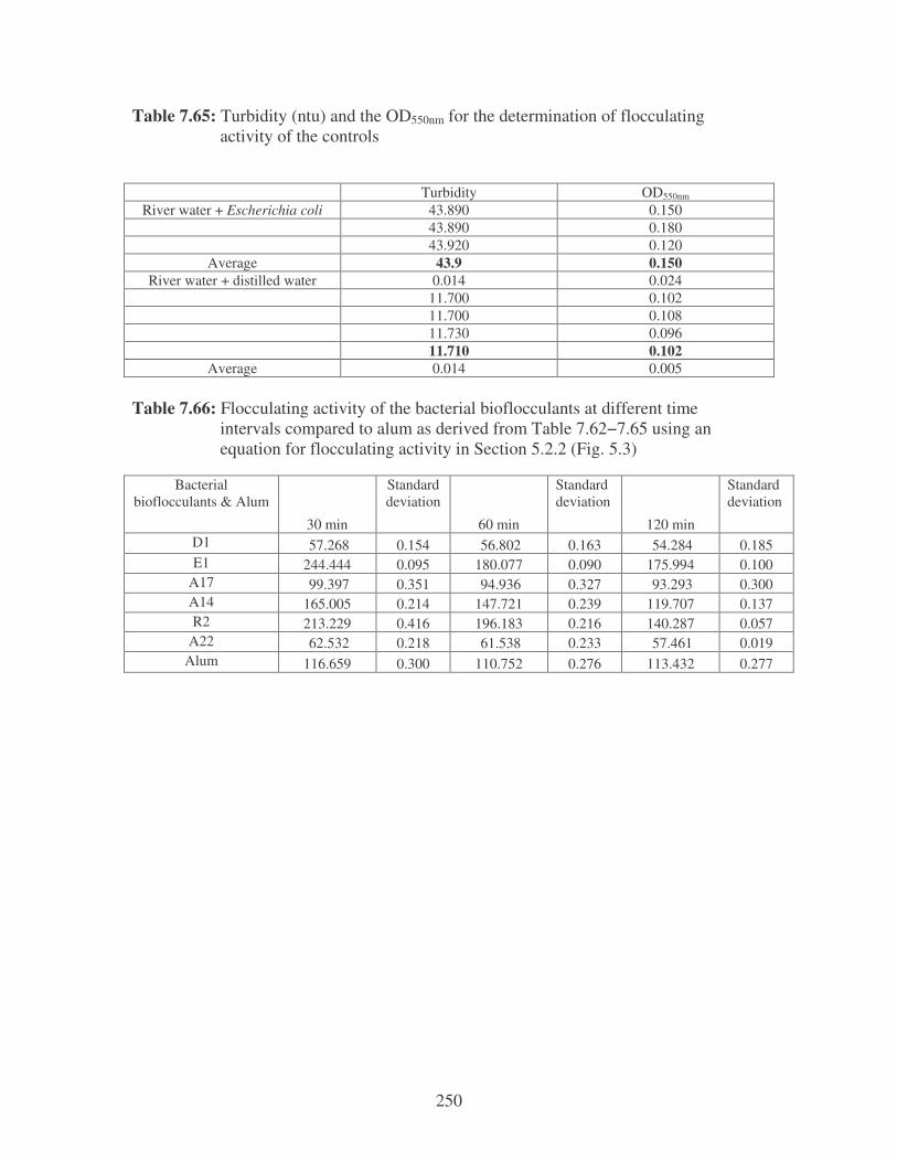
250
Table 7.65: Turbidity (ntu) and the OD550nm for the determination of flocculating activity of the controls Turbidity OD550nm
River water + Escherichia coli 43.890 0.150 43.890 0.180 43.920 0.120
Average 43.9 0.150 River water + distilled water 0.014 0.024
11.700 0.102 11.700 0.108 11.730 0.096 11.710 0.102
Average 0.014 0.005 Table 7.66: Flocculating activity of the bacterial bioflocculants at different time intervals compared to alum as derived from Table 7.62−7.65 using an equation for flocculating activity in Section 5.2.2 (Fig. 5.3)
Bacterial bioflocculants & Alum
30 min
Standard deviation
60 min
Standard deviation
120 min
Standard deviation
D1 57.268 0.154 56.802 0.163 54.284 0.185 E1 244.444 0.095 180.077 0.090 175.994 0.100
A17 99.397 0.351 94.936 0.327 93.293 0.300 A14 165.005 0.214 147.721 0.239 119.707 0.137 R2 213.229 0.416 196.183 0.216 140.287 0.057
A22 62.532 0.218 61.538 0.233 57.461 0.019 Alum 116.659 0.300 110.752 0.276 113.432 0.277
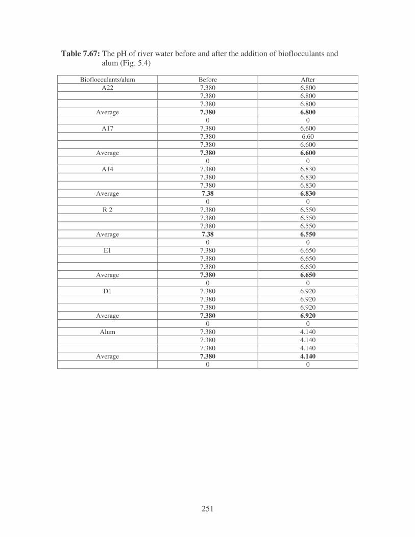
251
Table 7.67: The pH of river water before and after the addition of bioflocculants and alum (Fig. 5.4)
Bioflocculants/alum Before After A22 7.380 6.800
7.380 6.800 7.380 6.800
Average 7.380 6.800 0 0
A17 7.380 6.600 7.380 6.60 7.380 6.600
Average 7.380 6.600 0 0
A14 7.380 6.830 7.380 6.830 7.380 6.830
Average 7.38 6.830 0 0
R 2 7.380 6.550 7.380 6.550 7.380 6.550
Average 7.38 6.550 0 0
E1 7.380 6.650 7.380 6.650 7.380 6.650
Average 7.380 6.650 0 0
D1 7.380 6.920 7.380 6.920 7.380 6.920
Average 7.380 6.920 0 0
Alum 7.380 4.140 7.380 4.140 7.380 4.140
Average 7.380 4.140 0 0
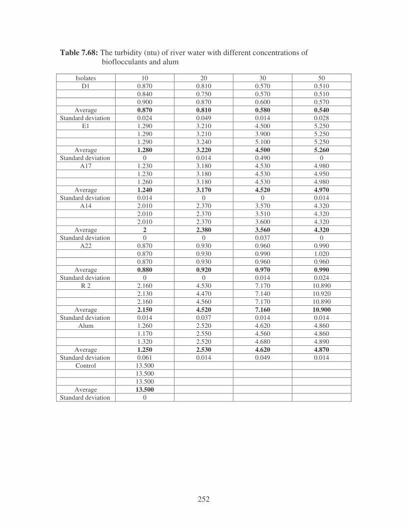
252
Table 7.68: The turbidity (ntu) of river water with different concentrations of bioflocculants and alum
Isolates 10 20 30 50 D1 0.870 0.810 0.570 0.510
0.840 0.750 0.570 0.510 0.900 0.870 0.600 0.570
Average 0.870 0.810 0.580 0.540 Standard deviation 0.024 0.049 0.014 0.028
E1 1.290 3.210 4.500 5.250 1.290 3.210 3.900 5.250 1.290 3.240 5.100 5.250
Average 1.280 3.220 4.500 5.260 Standard deviation 0 0.014 0.490 0
A17 1.230 3.180 4.530 4.980 1.230 3.180 4.530 4.950 1.260 3.180 4.530 4.980
Average 1.240 3.170 4.520 4.970 Standard deviation 0.014 0 0 0.014
A14 2.010 2.370 3.570 4.320 2.010 2.370 3.510 4.320 2.010 2.370 3.600 4.320
Average 2 2.380 3.560 4.320 Standard deviation 0 0 0.037 0
A22 0.870 0.930 0.960 0.990 0.870 0.930 0.990 1.020 0.870 0.930 0.960 0.960
Average 0.880 0.920 0.970 0.990 Standard deviation 0 0 0.014 0.024
R 2 2.160 4.530 7.170 10.890 2.130 4.470 7.140 10.920 2.160 4.560 7.170 10.890
Average 2.150 4.520 7.160 10.900 Standard deviation 0.014 0.037 0.014 0.014
Alum 1.260 2.520 4.620 4.860 1.170 2.550 4.560 4.860 1.320 2.520 4.680 4.890
Average 1.250 2.530 4.620 4.870 Standard deviation 0.061 0.014 0.049 0.014
Control 13.500 13.500 13.500
Average 13.500 Standard deviation 0
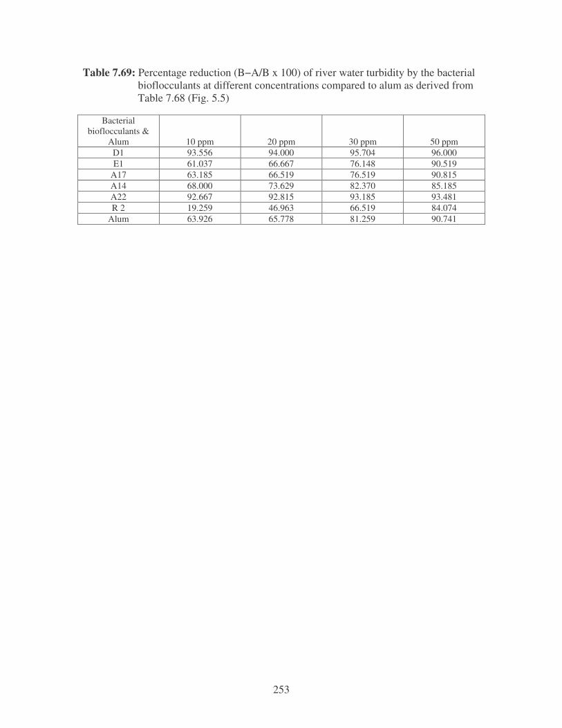
253
Table 7.69: Percentage reduction (B−A/B x 100) of river water turbidity by the bacterial bioflocculants at different concentrations compared to alum as derived from Table 7.68 (Fig. 5.5)
Bacterial bioflocculants &
Alum 10 ppm 20 ppm 30 ppm 50 ppm D1 93.556 94.000 95.704 96.000 E1 61.037 66.667 76.148 90.519
A17 63.185 66.519 76.519 90.815 A14 68.000 73.629 82.370 85.185 A22 92.667 92.815 93.185 93.481 R 2 19.259 46.963 66.519 84.074
Alum 63.926 65.778 81.259 90.741
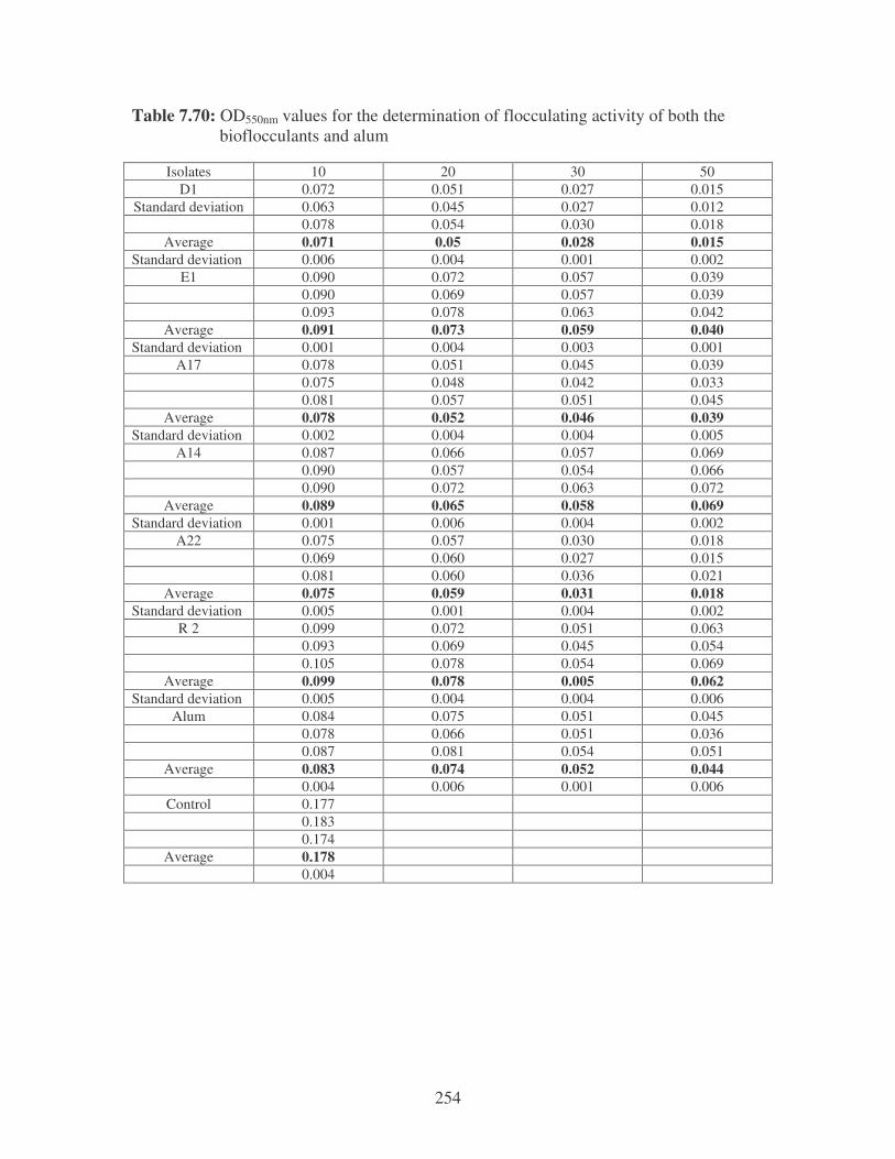
254
Table 7.70: OD550nm values for the determination of flocculating activity of both the bioflocculants and alum
Isolates 10 20 30 50 D1 0.072 0.051 0.027 0.015
Standard deviation 0.063 0.045 0.027 0.012 0.078 0.054 0.030 0.018
Average 0.071 0.05 0.028 0.015 Standard deviation 0.006 0.004 0.001 0.002
E1 0.090 0.072 0.057 0.039 0.090 0.069 0.057 0.039 0.093 0.078 0.063 0.042
Average 0.091 0.073 0.059 0.040 Standard deviation 0.001 0.004 0.003 0.001
A17 0.078 0.051 0.045 0.039 0.075 0.048 0.042 0.033 0.081 0.057 0.051 0.045
Average 0.078 0.052 0.046 0.039 Standard deviation 0.002 0.004 0.004 0.005
A14 0.087 0.066 0.057 0.069 0.090 0.057 0.054 0.066 0.090 0.072 0.063 0.072
Average 0.089 0.065 0.058 0.069 Standard deviation 0.001 0.006 0.004 0.002
A22 0.075 0.057 0.030 0.018 0.069 0.060 0.027 0.015 0.081 0.060 0.036 0.021
Average 0.075 0.059 0.031 0.018 Standard deviation 0.005 0.001 0.004 0.002
R 2 0.099 0.072 0.051 0.063 0.093 0.069 0.045 0.054 0.105 0.078 0.054 0.069
Average 0.099 0.078 0.005 0.062 Standard deviation 0.005 0.004 0.004 0.006
Alum 0.084 0.075 0.051 0.045 0.078 0.066 0.051 0.036 0.087 0.081 0.054 0.051
Average 0.083 0.074 0.052 0.044 0.004 0.006 0.001 0.006
Control 0.177 0.183 0.174
Average 0.178 0.004
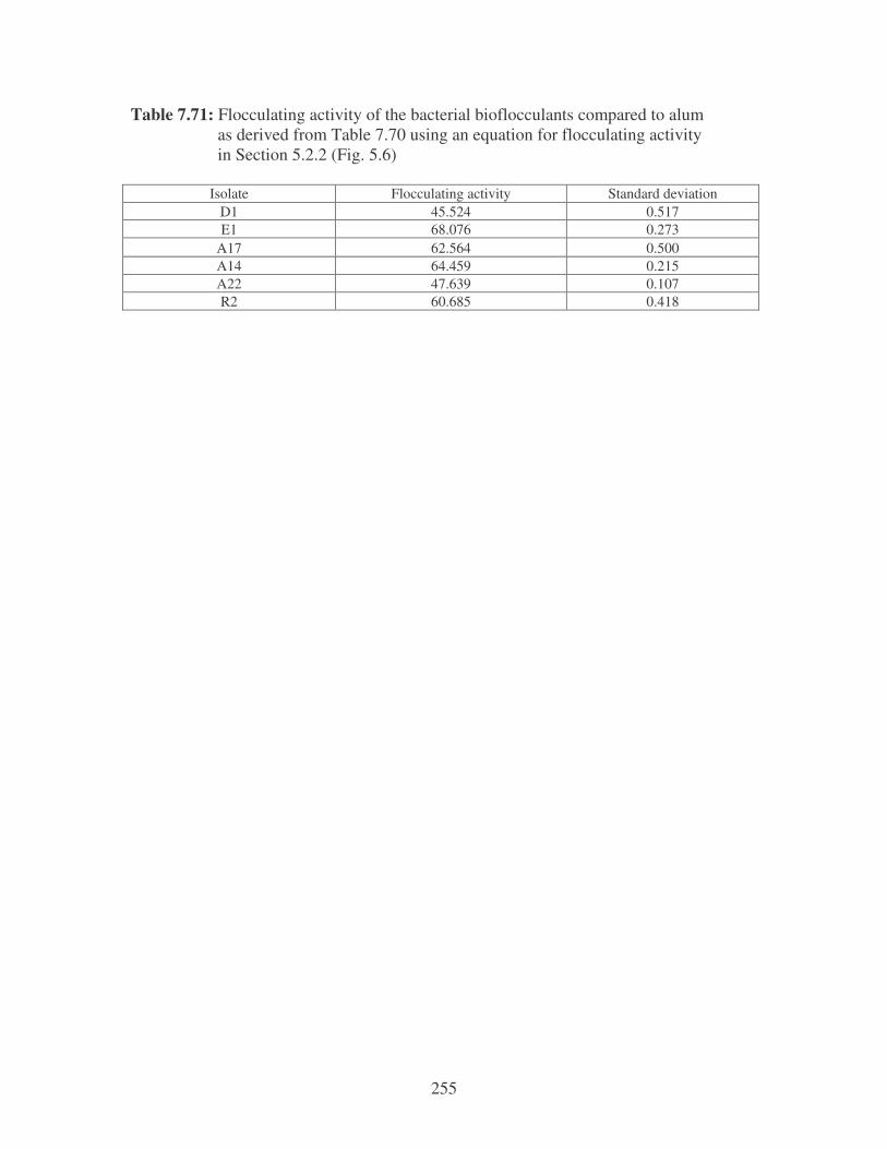
255
Table 7.71: Flocculating activity of the bacterial bioflocculants compared to alum as derived from Table 7.70 using an equation for flocculating activity in Section 5.2.2 (Fig. 5.6)
Isolate Flocculating activity Standard deviation D1 45.524 0.517 E1 68.076 0.273
A17 62.564 0.500 A14 64.459 0.215 A22 47.639 0.107 R2 60.685 0.418
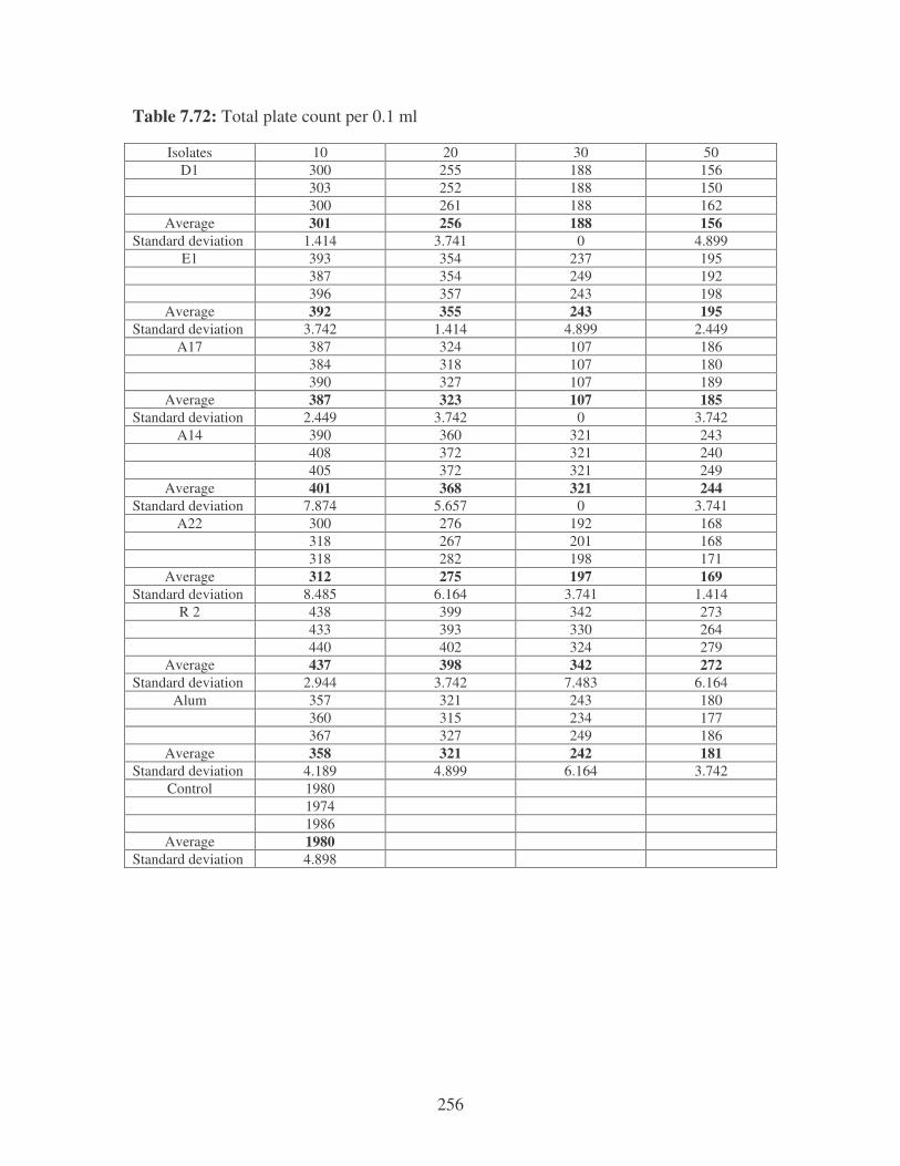
256
Table 7.72: Total plate count per 0.1 ml
Isolates 10 20 30 50 D1 300 255 188 156
303 252 188 150 300 261 188 162
Average 301 256 188 156 Standard deviation 1.414 3.741 0 4.899
E1 393 354 237 195 387 354 249 192 396 357 243 198
Average 392 355 243 195 Standard deviation 3.742 1.414 4.899 2.449
A17 387 324 107 186 384 318 107 180 390 327 107 189
Average 387 323 107 185 Standard deviation 2.449 3.742 0 3.742
A14 390 360 321 243 408 372 321 240 405 372 321 249
Average 401 368 321 244 Standard deviation 7.874 5.657 0 3.741
A22 300 276 192 168 318 267 201 168 318 282 198 171
Average 312 275 197 169 Standard deviation 8.485 6.164 3.741 1.414
R 2 438 399 342 273 433 393 330 264 440 402 324 279
Average 437 398 342 272 Standard deviation 2.944 3.742 7.483 6.164
Alum 357 321 243 180 360 315 234 177 367 327 249 186
Average 358 321 242 181 Standard deviation 4.189 4.899 6.164 3.742
Control 1980 1974 1986
Average 1980 Standard deviation 4.898
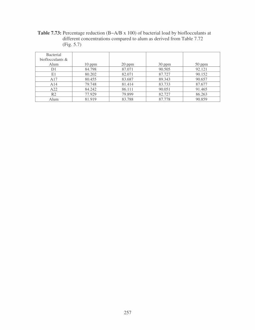
257
Table 7.73: Percentage reduction (B−A/B x 100) of bacterial load by bioflocculants at different concentrations compared to alum as derived from Table 7.72 (Fig. 5.7)
Bacterial bioflocculants &
Alum 10 ppm 20 ppm 30 ppm 50 ppm D1 84.798 87.071 90.505 92.121 E1 80.202 82.071 87.727 90.152
A17 80.455 83.687 89.343 90.657 A14 79.748 81.414 83.733 87.677 A22 84.242 86.111 90.051 91.465 R2 77.929 79.899 82.727 86.263
Alum 81.919 83.788 87.778 90.859
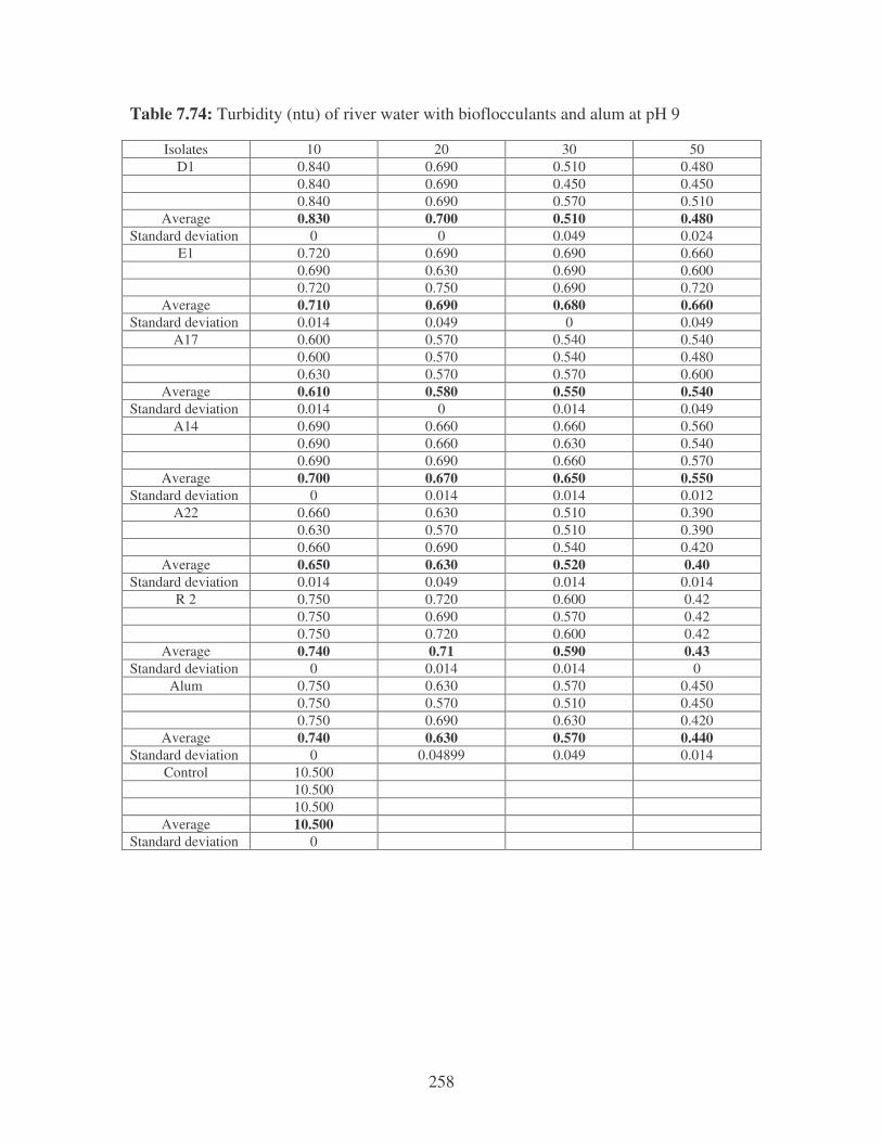
258
Table 7.74: Turbidity (ntu) of river water with bioflocculants and alum at pH 9
Isolates 10 20 30 50 D1 0.840 0.690 0.510 0.480
0.840 0.690 0.450 0.450 0.840 0.690 0.570 0.510
Average 0.830 0.700 0.510 0.480 Standard deviation 0 0 0.049 0.024
E1 0.720 0.690 0.690 0.660 0.690 0.630 0.690 0.600 0.720 0.750 0.690 0.720
Average 0.710 0.690 0.680 0.660 Standard deviation 0.014 0.049 0 0.049
A17 0.600 0.570 0.540 0.540 0.600 0.570 0.540 0.480 0.630 0.570 0.570 0.600
Average 0.610 0.580 0.550 0.540 Standard deviation 0.014 0 0.014 0.049
A14 0.690 0.660 0.660 0.560 0.690 0.660 0.630 0.540 0.690 0.690 0.660 0.570
Average 0.700 0.670 0.650 0.550 Standard deviation 0 0.014 0.014 0.012
A22 0.660 0.630 0.510 0.390 0.630 0.570 0.510 0.390 0.660 0.690 0.540 0.420
Average 0.650 0.630 0.520 0.40 Standard deviation 0.014 0.049 0.014 0.014
R 2 0.750 0.720 0.600 0.42 0.750 0.690 0.570 0.42 0.750 0.720 0.600 0.42
Average 0.740 0.71 0.590 0.43 Standard deviation 0 0.014 0.014 0
Alum 0.750 0.630 0.570 0.450 0.750 0.570 0.510 0.450 0.750 0.690 0.630 0.420
Average 0.740 0.630 0.570 0.440 Standard deviation 0 0.04899 0.049 0.014
Control 10.500 10.500 10.500
Average 10.500 Standard deviation 0
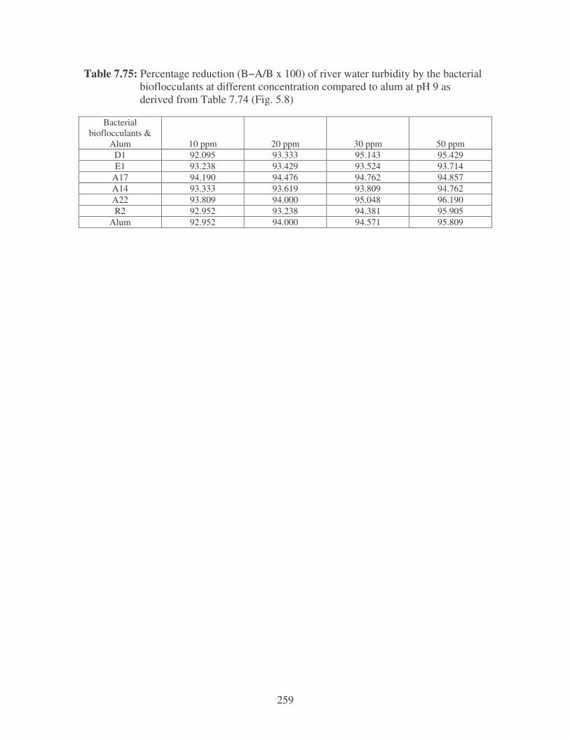
259
Table 7.75: Percentage reduction (B−A/B x 100) of river water turbidity by the bacterial bioflocculants at different concentration compared to alum at pH 9 as derived from Table 7.74 (Fig. 5.8)
Bacterial bioflocculants &
Alum 10 ppm 20 ppm 30 ppm 50 ppm D1 92.095 93.333 95.143 95.429 E1 93.238 93.429 93.524 93.714
A17 94.190 94.476 94.762 94.857 A14 93.333 93.619 93.809 94.762 A22 93.809 94.000 95.048 96.190 R2 92.952 93.238 94.381 95.905
Alum 92.952 94.000 94.571 95.809
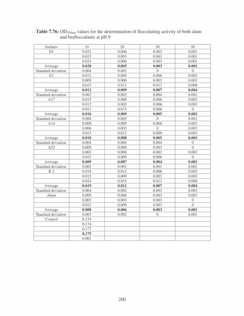
260
Table 7.76: OD550nm values for the determination of flocculating activity of both alum and bioflocculants at pH 9
Isolates 10 20 30 50 D1 0.021 0.006 0.003 0.001
0.015 0.003 0.003 0.001 0.024 0.006 0.003 0.001
Average 0.020 0.005 0.003 0.001 Standard deviation 0.004 0.001 0 0
E1 0.012 0.009 0.006 0.003 0.009 0.006 0.003 0.003 0.015 0.012 0.012 0.006
Average 0.012 0.009 0.007 0.004 Standard deviation 0.002 0.002 0.004 0.001
A17 0.015 0.009 0.006 0.003 0.012 0.003 0.006 0.003 0.021 0.015 0.006 0
Average 0.016 0.009 0.005 0.002 Standard deviation 0.004 0.005 0 0.001
A14 0.009 0.009 0.006 0.003 0.006 0.003 0 0.003 0.015 0.012 0.009 0.003
Average 0.010 0.008 0.005 0.003 Standard deviation 0.004 0.004 0.004 0
A22 0.009 0.006 0.003 0 0.003 0.006 0.003 0.003 0.015 0.009 0.006 0
Average 0.009 0.007 0.004 0.001 Standard deviation 0.005 0.001 0.001 0.001
R 2 0.018 0.012 0.006 0.003 0.015 0.009 0.003 0.003 0.024 0.015 0.012 0.006
Average 0.019 0.012 0.007 0.004 Standard deviation 0.004 0.002 0.003 0.001
Alum 0.009 0.006 0.003 0.003 0.003 0.003 0.003 0 0.012 0.009 0.003 0
Average 0.008 0.006 0.003 0.001 Standard deviation 0.003 0.002 0 0.001
Control 0.174 0.174 0.177 0.175
0.001
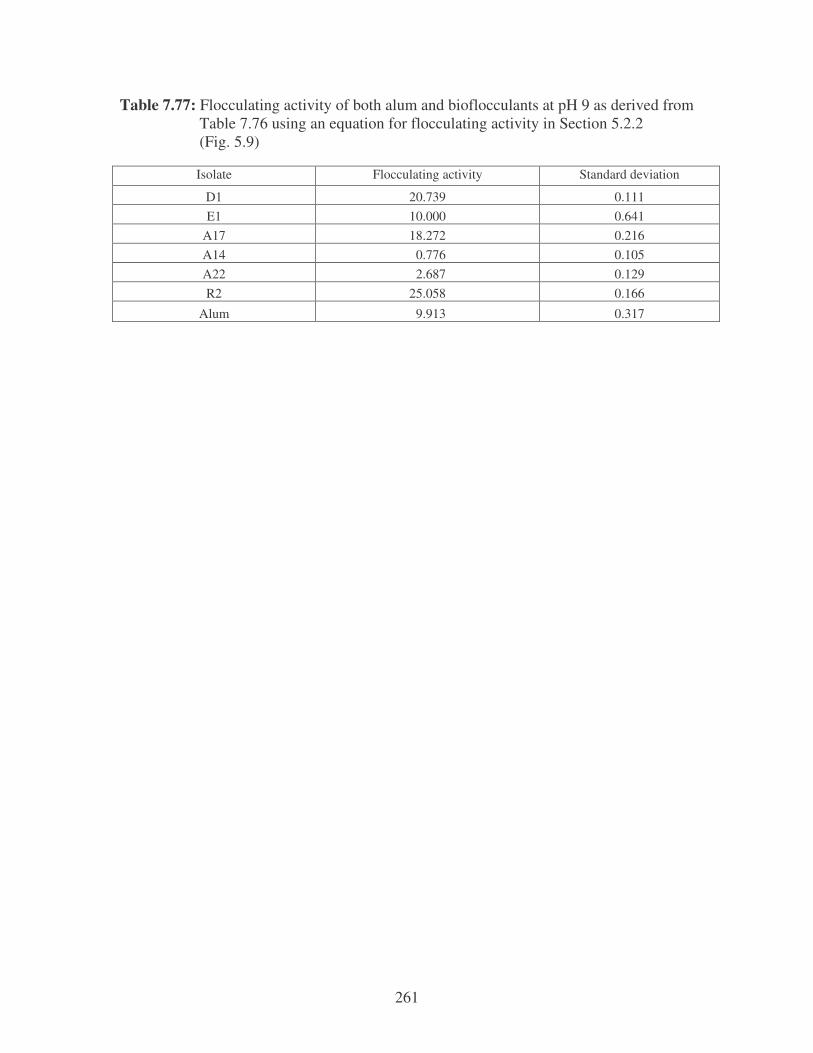
261
Table 7.77: Flocculating activity of both alum and bioflocculants at pH 9 as derived from Table 7.76 using an equation for flocculating activity in Section 5.2.2 (Fig. 5.9)
Isolate Flocculating activity Standard deviation
D1 20.739 0.111 E1 10.000 0.641
A17 18.272 0.216 A14 0.776 0.105 A22 2.687 0.129 R2 25.058 0.166
Alum 9.913 0.317
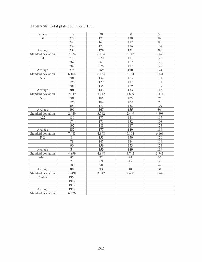
262
Table 7.78: Total plate count per 0.1 ml
Isolates 10 20 30 50 D1 222 171 120 99
240 162 117 93 237 177 126 102
Average 233 170 121 98 Standard deviation 7.874 6.164 3.742 3.742
E1 276 270 171 123 267 261 162 120 282 276 177 129
Average 275 269 170 124 Standard deviation 6.164 6.164 6.164 3.741
A17 201 132 123 114 198 129 117 114 204 138 129 117
Average 201 133 123 115 Standard deviation 2.449 3.742 4.899 1.414
A14 201 168 135 96 198 162 132 90 204 171 138 102
Average 199 167 135 96 Standard deviation 2.449 3.742 2.449 4.898
A22 180 177 141 117 174 171 132 108 192 183 147 123
Average 182 177 140 116 Standard deviation 7.483 4.898 6.164 6.164
R 2 84 153 150 120 78 147 144 114 90 159 153 123
Average 84 153 149 119 Standard deviation 4.899 4.898 3.742 3.742
Alum 87 72 48 36 72 69 45 33 105 78 51 42
Average 88 73 48 37 Standard deviation 13.491 3.742 2.450 3.742
Control 1965 1982 1972
Average 1978 Standard deviation 6.976
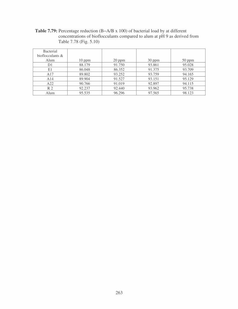
263
Table 7.79: Percentage reduction (B−A/B x 100) of bacterial load by at different concentrations of bioflocculants compared to alum at pH 9 as derived from Table 7.78 (Fig. 5.10)
Bacterial bioflocculants &
Alum 10 ppm 20 ppm 30 ppm 50 ppm D1 88.179 91.750 93.861 95.028 E1 86.048 86.352 91.375 93.709
A17 89.802 93.252 93.759 94.165 A14 89.904 91.527 93.151 95.129 A22 90.766 91.019 92.897 94.115 R 2 92.237 92.440 93.962 95.738
Alum 95.535 96.296 97.565 98.123
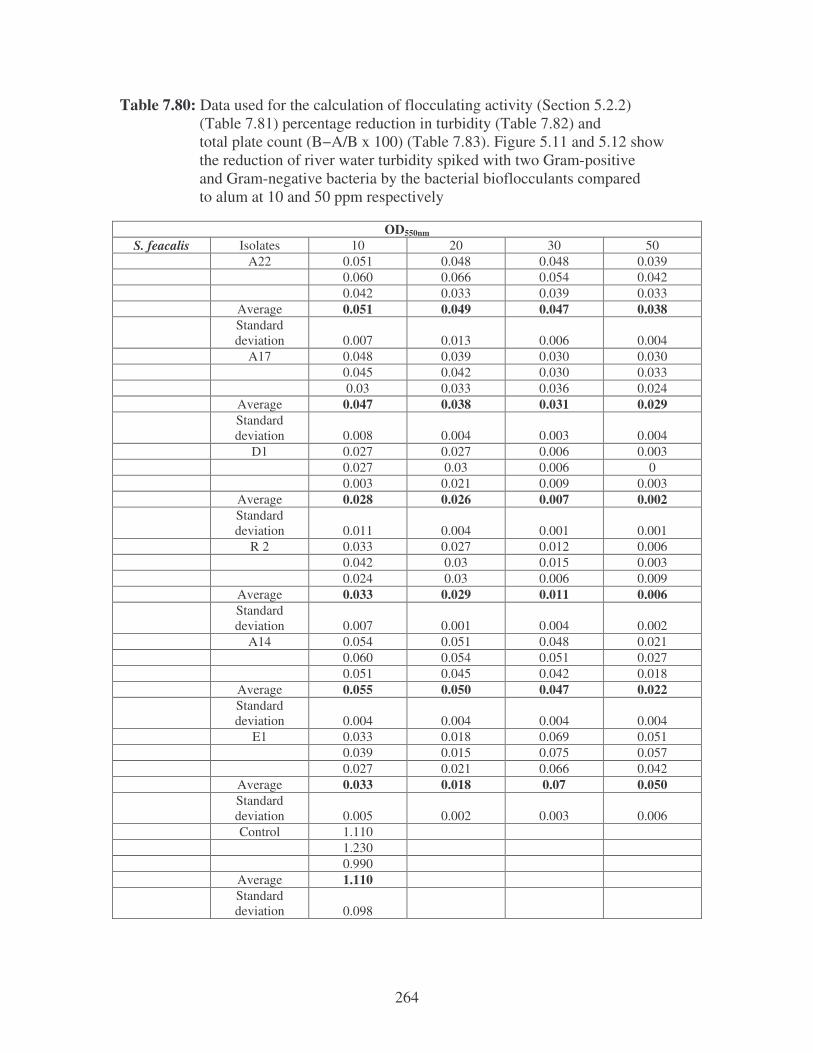
264
Table 7.80: Data used for the calculation of flocculating activity (Section 5.2.2) (Table 7.81) percentage reduction in turbidity (Table 7.82) and total plate count (B−A/B x 100) (Table 7.83). Figure 5.11 and 5.12 show the reduction of river water turbidity spiked with two Gram-positive and Gram-negative bacteria by the bacterial bioflocculants compared to alum at 10 and 50 ppm respectively
OD550nm S. feacalis Isolates 10 20 30 50
A22 0.051 0.048 0.048 0.039 0.060 0.066 0.054 0.042 0.042 0.033 0.039 0.033 Average 0.051 0.049 0.047 0.038
Standard deviation 0.007 0.013 0.006 0.004
A17 0.048 0.039 0.030 0.030 0.045 0.042 0.030 0.033 0.03 0.033 0.036 0.024 Average 0.047 0.038 0.031 0.029
Standard deviation 0.008 0.004 0.003 0.004
D1 0.027 0.027 0.006 0.003 0.027 0.03 0.006 0 0.003 0.021 0.009 0.003 Average 0.028 0.026 0.007 0.002
Standard deviation 0.011 0.004 0.001 0.001
R 2 0.033 0.027 0.012 0.006 0.042 0.03 0.015 0.003 0.024 0.03 0.006 0.009 Average 0.033 0.029 0.011 0.006
Standard deviation 0.007 0.001 0.004 0.002
A14 0.054 0.051 0.048 0.021 0.060 0.054 0.051 0.027 0.051 0.045 0.042 0.018 Average 0.055 0.050 0.047 0.022
Standard deviation 0.004 0.004 0.004 0.004
E1 0.033 0.018 0.069 0.051 0.039 0.015 0.075 0.057 0.027 0.021 0.066 0.042 Average 0.033 0.018 0.07 0.050
Standard deviation 0.005 0.002 0.003 0.006
Control 1.110 1.230 0.990 Average 1.110
Standard deviation 0.098
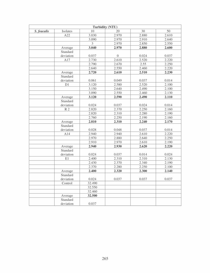
265
Turbidity (NTU) S. feacalis Isolates 10 20 30 50
A22 3.030 2.970 2.880 2.610 3.090 2.970 2.910 2.640 3 2.970 2.850 2.550 Average 3.040 2.970 2.880 2.600
Standard deviation 0.037 0 0.024 0.037
A17 2.730 2.610 2.520 2.220 2.790 2.670 2.55 2.250 2.640 2.550 2.460 2.220 Average 2.720 2.610 2.510 2.230
Standard deviation 0.061 0.049 0.037 0.014
D1 3.120 2.580 2.520 2.100 3.150 2.640 2.490 2.100 3.090 2.550 2.460 2.130 Average 3.120 2.590 2.490 2.110
Standard deviation 0.024 0.037 0.024 0.014
R 2 2.820 2.370 2.250 2.160 2.820 2.310 2.280 2.190 2.760 2.250 2.190 2.160 Average 2.810 2.310 2.240 2.170
Standard deviation 0.028 0.048 0.037 0.014
A14 2.940 2.940 2.610 2.220 2.970 2.880 2.640 2.250 2.910 2.970 2.610 2.190 Average 2.940 2.930 2.620 2.220
Standard deviation 0.024 0.037 0.014 0.024
E1 2.400 2.310 2.310 2.130 2.430 2.370 2.340 2.190 2.370 2.280 2.250 2.100 Average 2.400 2.320 2.300 2.140
Standard deviation 0.024 0.037 0.037 0.037
Control 32.490 32.550 32.460 Average 32.500
Standard deviation 0.037

266
Plate count per 0.1 ml S. feacalis Isolates 10 20 30 50
A22 6 3 1 0 3 2 1 0 0 1 1 0 Average 3 2 1 0
Standard deviation 2.449 0.816 0 0
A17 6 9 9 5 9 6 3 3 6 3 3 3 Average 7 6 5 4
Standard deviation 1.414 2.449 2.828 0.942
D1 138 114 105 81 135 117 99 87 138 114 95 78 Average 137 115 98 82
Standard deviation 1.414 1.414 4.109 3.742
R 2 69 55 9 3 70 50 3 3 71 51 9 0 Average 70 52 7 2
Standard deviation 0.816 2.160 2.828 1.414
A14 126 1 1 0 130 1 1 0 122 1 1 0 Average 126 1 1 0
Standard deviation 3.265 0 0 0
E1 18 3 3 1 19 3 3 1 20 3 0 1 Average 19 3 2 1
Standard deviation 0.816 0 1.414 0
Control 180 183 183 Average 182
Standard deviation
1.414
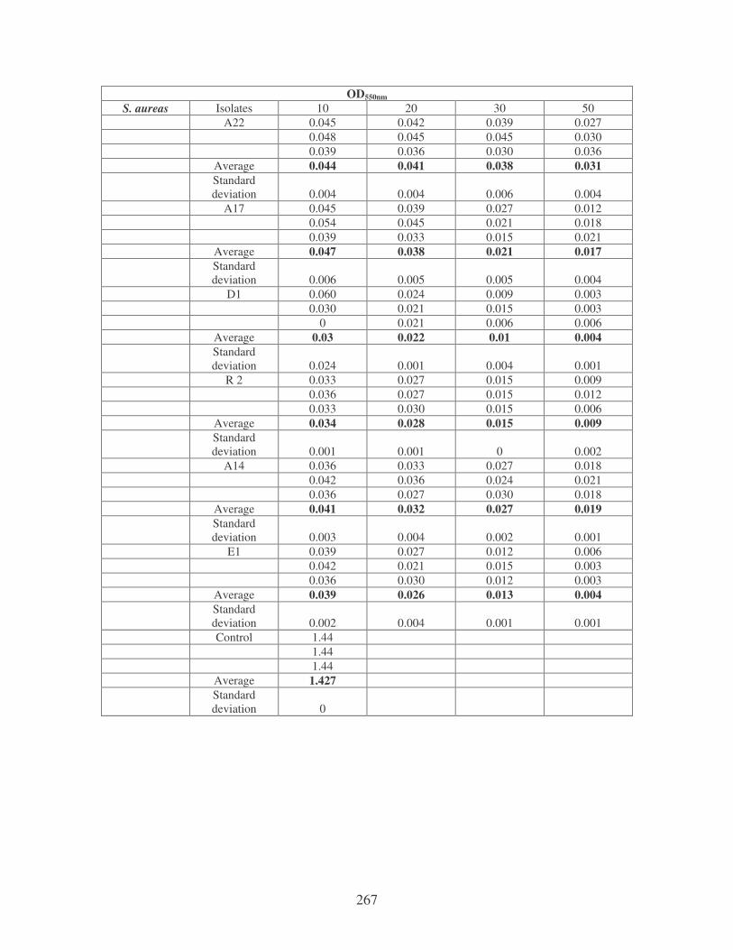
267
OD550nm S. aureas Isolates 10 20 30 50
A22 0.045 0.042 0.039 0.027 0.048 0.045 0.045 0.030 0.039 0.036 0.030 0.036 Average 0.044 0.041 0.038 0.031
Standard deviation 0.004 0.004 0.006 0.004
A17 0.045 0.039 0.027 0.012 0.054 0.045 0.021 0.018 0.039 0.033 0.015 0.021 Average 0.047 0.038 0.021 0.017
Standard deviation 0.006 0.005 0.005 0.004
D1 0.060 0.024 0.009 0.003 0.030 0.021 0.015 0.003 0 0.021 0.006 0.006 Average 0.03 0.022 0.01 0.004
Standard deviation 0.024 0.001 0.004 0.001
R 2 0.033 0.027 0.015 0.009 0.036 0.027 0.015 0.012 0.033 0.030 0.015 0.006 Average 0.034 0.028 0.015 0.009
Standard deviation 0.001 0.001 0 0.002
A14 0.036 0.033 0.027 0.018 0.042 0.036 0.024 0.021 0.036 0.027 0.030 0.018 Average 0.041 0.032 0.027 0.019
Standard deviation 0.003 0.004 0.002 0.001
E1 0.039 0.027 0.012 0.006 0.042 0.021 0.015 0.003 0.036 0.030 0.012 0.003 Average 0.039 0.026 0.013 0.004
Standard deviation 0.002 0.004 0.001 0.001
Control 1.44 1.44 1.44 Average 1.427
Standard deviation 0
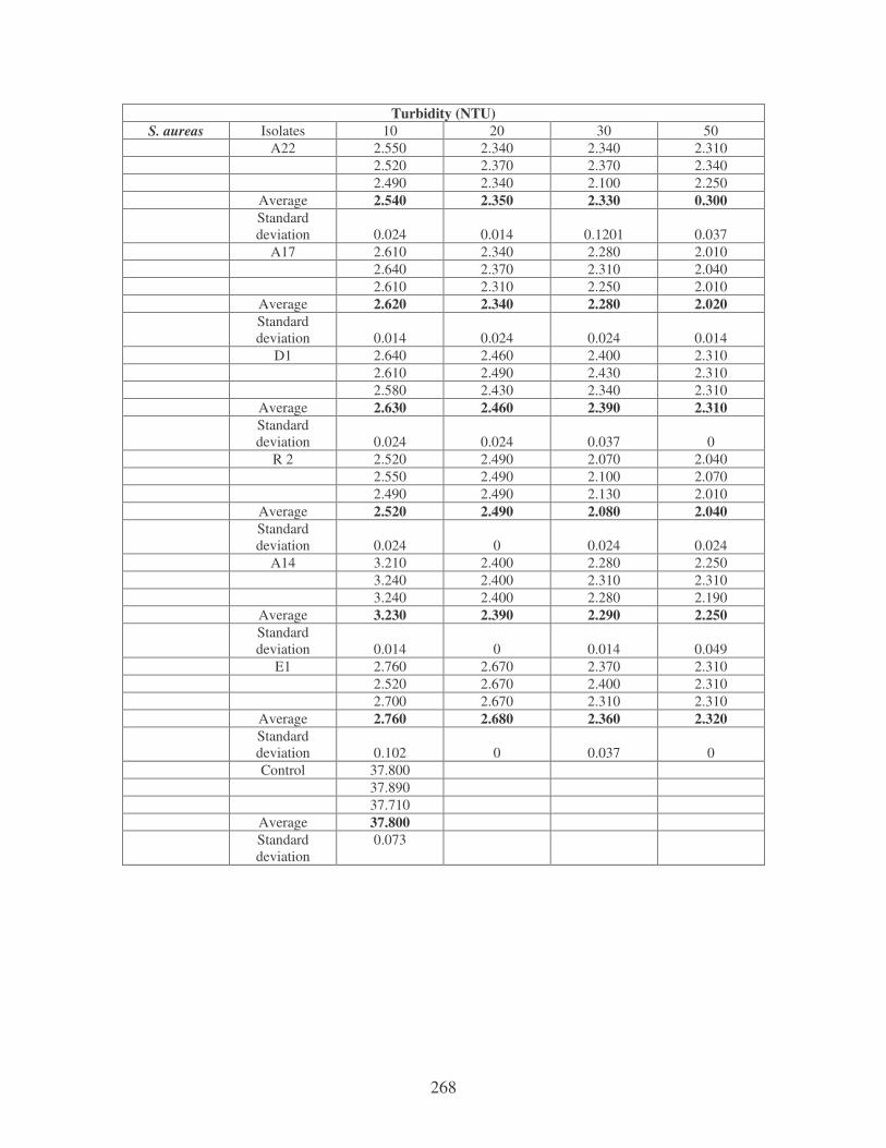
268
Turbidity (NTU) S. aureas Isolates 10 20 30 50
A22 2.550 2.340 2.340 2.310 2.520 2.370 2.370 2.340 2.490 2.340 2.100 2.250 Average 2.540 2.350 2.330 0.300
Standard deviation 0.024 0.014 0.1201 0.037
A17 2.610 2.340 2.280 2.010 2.640 2.370 2.310 2.040 2.610 2.310 2.250 2.010 Average 2.620 2.340 2.280 2.020
Standard deviation 0.014 0.024 0.024 0.014
D1 2.640 2.460 2.400 2.310 2.610 2.490 2.430 2.310 2.580 2.430 2.340 2.310 Average 2.630 2.460 2.390 2.310
Standard deviation 0.024 0.024 0.037 0
R 2 2.520 2.490 2.070 2.040 2.550 2.490 2.100 2.070 2.490 2.490 2.130 2.010 Average 2.520 2.490 2.080 2.040
Standard deviation 0.024 0 0.024 0.024
A14 3.210 2.400 2.280 2.250 3.240 2.400 2.310 2.310 3.240 2.400 2.280 2.190 Average 3.230 2.390 2.290 2.250
Standard deviation 0.014 0 0.014 0.049
E1 2.760 2.670 2.370 2.310 2.520 2.670 2.400 2.310 2.700 2.670 2.310 2.310 Average 2.760 2.680 2.360 2.320
Standard deviation 0.102 0 0.037 0
Control 37.800 37.890 37.710 Average 37.800
Standard deviation
0.073
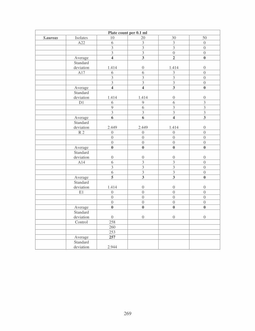
269
Plate count per 0.1 ml S.aureas Isolates 10 20 30 50
A22 6 3 3 0 3 3 3 0 3 3 0 0 Average 4 3 2 0
Standard deviation 1.414 0 1.414 0
A17 6 6 3 0 3 3 3 0 3 3 3 0 Average 4 4 3 0
Standard deviation 1.414 1.414 0 0
D1 6 9 6 3 9 6 3 3 3 3 3 3 Average 6 6 4 3
Standard deviation 2.449 2.449 1.414 0
R 2 0 0 0 0 0 0 0 0 0 0 0 0 Average 0 0 0 0
Standard deviation 0 0 0 0
A14 6 3 3 0 3 3 3 0 6 3 3 0 Average 5 3 3 0
Standard deviation 1.414 0 0 0
E1 0 0 0 0 0 0 0 0 0 0 0 0 Average 0 0 0 0
Standard deviation 0 0 0 0
Control 258 260 253 Average 257
Standard deviation 2.944
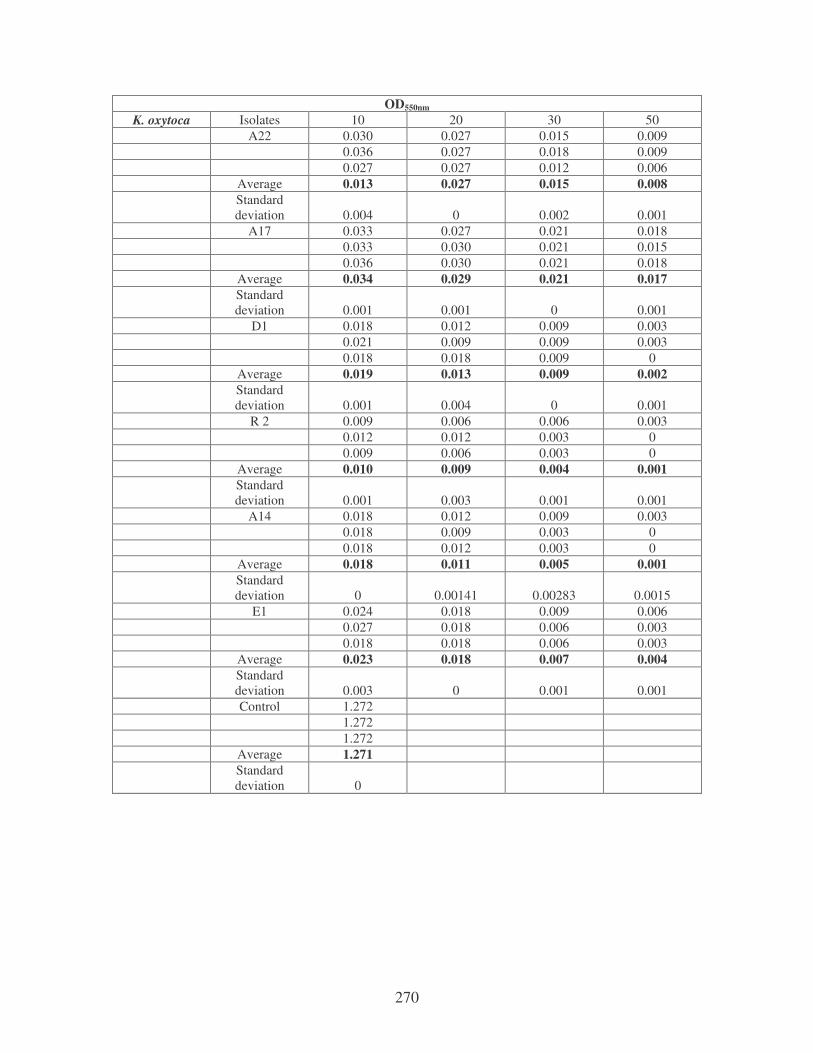
270
OD550nm K. oxytoca Isolates 10 20 30 50
A22 0.030 0.027 0.015 0.009 0.036 0.027 0.018 0.009 0.027 0.027 0.012 0.006 Average 0.013 0.027 0.015 0.008
Standard deviation 0.004 0 0.002 0.001
A17 0.033 0.027 0.021 0.018 0.033 0.030 0.021 0.015 0.036 0.030 0.021 0.018 Average 0.034 0.029 0.021 0.017
Standard deviation 0.001 0.001 0 0.001
D1 0.018 0.012 0.009 0.003 0.021 0.009 0.009 0.003 0.018 0.018 0.009 0 Average 0.019 0.013 0.009 0.002
Standard deviation 0.001 0.004 0 0.001
R 2 0.009 0.006 0.006 0.003 0.012 0.012 0.003 0 0.009 0.006 0.003 0 Average 0.010 0.009 0.004 0.001
Standard deviation 0.001 0.003 0.001 0.001
A14 0.018 0.012 0.009 0.003 0.018 0.009 0.003 0 0.018 0.012 0.003 0 Average 0.018 0.011 0.005 0.001
Standard deviation 0 0.00141 0.00283 0.0015
E1 0.024 0.018 0.009 0.006 0.027 0.018 0.006 0.003 0.018 0.018 0.006 0.003 Average 0.023 0.018 0.007 0.004
Standard deviation 0.003 0 0.001 0.001
Control 1.272 1.272 1.272 Average 1.271
Standard deviation 0
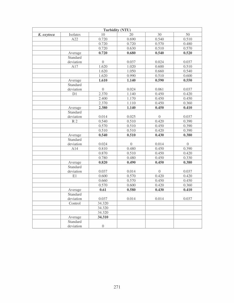
271
Turbidity (NTU) K. oxytoca Isolates 10 20 30 50
A22 0.720 0.690 0.540 0.510 0.720 0.720 0.570 0.480 0.720 0.630 0.510 0.570 Average 0.720 0.680 0.540 0.520
Standard deviation 0 0.037 0.024 0.037
A17 1.620 1.020 0.600 0.510 1.620 1.050 0.660 0.540 1.620 0.990 0.510 0.600 Average 1.610 1.140 0.590 0.550
Standard deviation 0 0.024 0.061 0.037
D1 2.370 1.140 0.450 0.420 2.400 1.170 0.450 0.450 2.370 1.110 0.450 0.360 Average 2.380 1.140 0.450 0.410
Standard deviation 0.014 0.025 0 0.037
R 2 0.540 0.510 0.420 0.390 0.570 0.510 0.450 0.390 0.510 0.510 0.420 0.390 Average 0.540 0.510 0.430 0.380
Standard deviation 0.024 0 0.014 0
A14 0.810 0.480 0.450 0.390 0.870 0.510 0.450 0.420 0.780 0.480 0.450 0.330 Average 0.820 0.490 0.450 0.380
Standard deviation 0.037 0.014 0 0.037
E1 0.600 0.570 0.420 0.420 0.660 0.570 0.450 0.450 0.570 0.600 0.420 0.360 Average 0.61 0.580 0.430 0.410
Standard deviation 0.037 0.014 0.014 0.037
Control 34.320 34.320 34.320 Average 34.310
Standard deviation 0

272
Plate count per 0.1 ml K. oxytoca Isolates 10 20 30 50
A22 12 9 3 3 6 7 2 0 6 5 1 0 Average 8 5 2 1
Standard deviation 2.828 1.633 0.817 1.414
A17 0 0 0 0 0 0 0 0 0 0 0 0 Average 0 0 0 0
Standard deviation 0 0 0 0
D1 15 12 12 6 20 13 15 9 13 14 9 6 Average 15 13 12 7
Standard deviation 2.944 0.817 2.449 1.414
R 2 12 9 6 3 12 6 5 3 14 6 4 0 Average 13 7 5 2
Standard deviation 0.942 1.414 0.817 1.414
A14 6 3 1 0 3 3 1 0 3 3 1 0 Average 4 3 1 0
Standard deviation 1.414 0 0 0
E1 0 0 0 0 0 0 0 0 0 0 0 0 Average 0 0 0 0
Standard deviation 0 0 0 0
Control 210 215 208 Average 211
Standard deviation 2.944
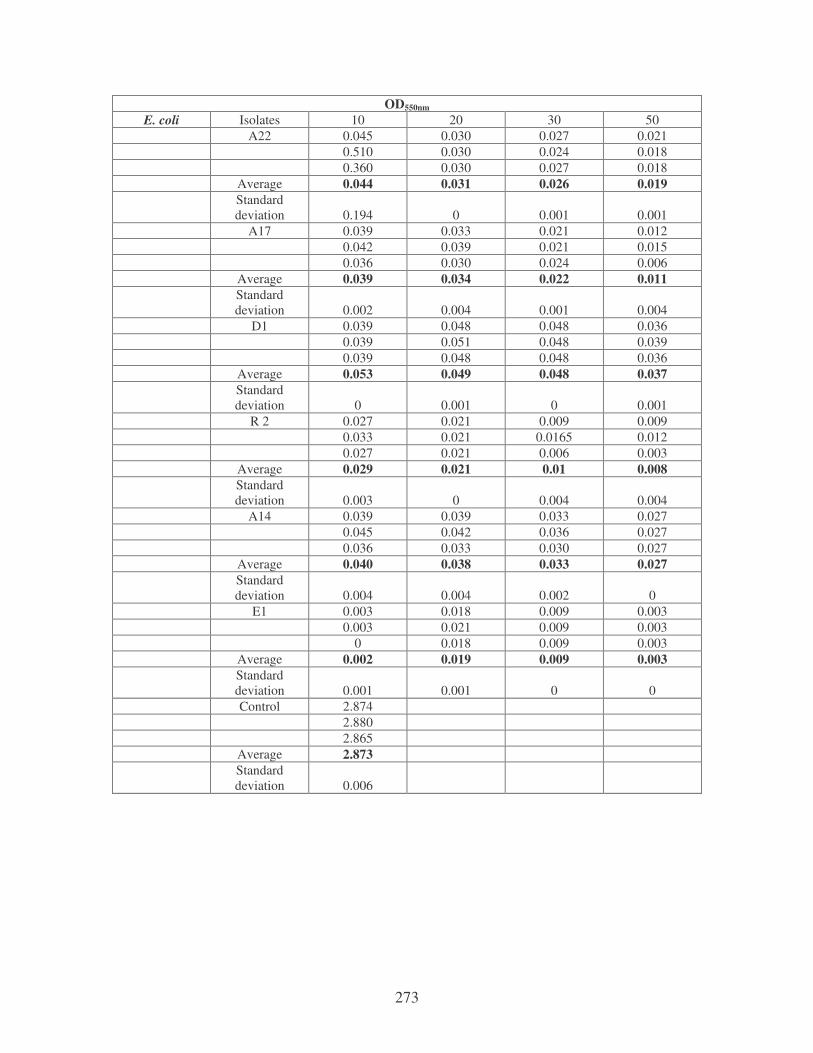
273
OD550nm E. coli Isolates 10 20 30 50
A22 0.045 0.030 0.027 0.021 0.510 0.030 0.024 0.018 0.360 0.030 0.027 0.018 Average 0.044 0.031 0.026 0.019
Standard deviation 0.194 0 0.001 0.001
A17 0.039 0.033 0.021 0.012 0.042 0.039 0.021 0.015 0.036 0.030 0.024 0.006 Average 0.039 0.034 0.022 0.011
Standard deviation 0.002 0.004 0.001 0.004
D1 0.039 0.048 0.048 0.036 0.039 0.051 0.048 0.039 0.039 0.048 0.048 0.036 Average 0.053 0.049 0.048 0.037
Standard deviation 0 0.001 0 0.001
R 2 0.027 0.021 0.009 0.009 0.033 0.021 0.0165 0.012 0.027 0.021 0.006 0.003 Average 0.029 0.021 0.01 0.008
Standard deviation 0.003 0 0.004 0.004
A14 0.039 0.039 0.033 0.027 0.045 0.042 0.036 0.027 0.036 0.033 0.030 0.027 Average 0.040 0.038 0.033 0.027
Standard deviation 0.004 0.004 0.002 0
E1 0.003 0.018 0.009 0.003 0.003 0.021 0.009 0.003 0 0.018 0.009 0.003 Average 0.002 0.019 0.009 0.003
Standard deviation 0.001 0.001 0 0
Control 2.874 2.880 2.865 Average 2.873
Standard deviation 0.006
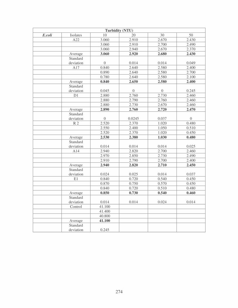
274
Turbidity (NTU) E.coli Isolates 10 20 30 50
A22 3.060 2.910 2.670 2.430 3.060 2.910 2.700 2.490 3.060 2.940 2.670 2.370 Average 3.060 2.920 2.680 2.430
Standard deviation 0 0.014 0.014 0.049
A17 0.840 2.640 2.580 2.400 0.890 2.640 2.580 2.700 0.780 2.640 2.580 2.100 Average 0.840 2.650 2.580 2.400
Standard deviation 0.045 0 0 0.245
D1 2.880 2.760 2.730 2.460 2.880 2.790 2.760 2.460 2.880 2.730 2.670 2.460 Average 2.890 2.760 2.720 2.470
Standard deviation 0 0.0245 0.037 0
R 2 2.520 2.370 1.020 0.480 2.550 2.400 1.050 0.510 2.520 2.370 1.020 0.450 Average 2.530 2.380 1.030 0.480
Standard deviation 0.014 0.014 0.014 0.025
A14 2.940 2.820 2.700 2.460 2.970 2.850 2.730 2.490 2.910 2.790 2.700 2.400 Average 2.940 2.820 2.710 2.450
Standard deviation 0.024 0.025 0.014 0.037
E1 0.840 0.720 0.540 0.450 0.870 0.750 0.570 0.450 0.840 0.720 0.510 0.480 Average 0.850 0.730 0.540 0.460
Standard deviation 0.014 0.014 0.024 0.014
Control 41.100 41.400 40.800 Average 41.100
Standard deviation 0.245
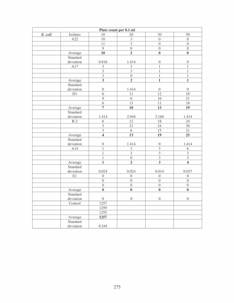
275
Plate count per 0.1 ml E. coli Isolates 10 20 30 50
A22 10 3 0 0 11 3 0 0 9 0 0 0 Average 10 2 0 0
Standard deviation 0.816 1.414 0 0
A17 3 3 1 1 3 3 1 1 3 0 1 1 Average 3 2 1 1
Standard deviation 0 1.414 0 0
D1 6 11 12 18 9 6 16 21 6 13 11 18 Average 7 10 13 19
Standard deviation 1.414 2.944 2.160 1.414
R 2 6 12 18 24 3 21 24 30 3 6 15 21 Average 4 13 19 25
Standard deviation 0 1.414 0 1.414
A14 1 3 3 6 1 3 3 3 1 0 3 3 Average 1 2 3 4
Standard deviation 0.024 0.024 0.014 0.037
E1 0 0 0 0 0 0 0 0 0 0 0 0 Average 0 0 0 0
Standard deviation 0 0 0 0
Control 1257 1259 1255 Average 1257
Standard deviation 0.245
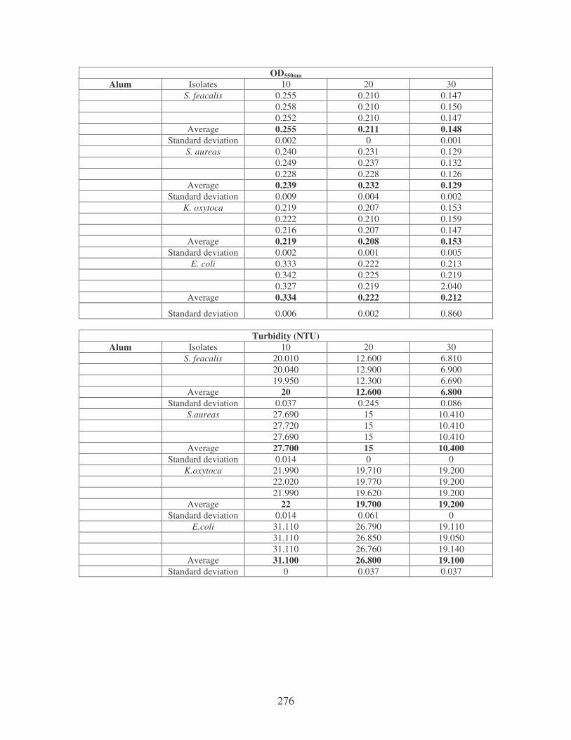
276
OD550nm Alum Isolates 10 20 30
S. feacalis 0.255 0.210 0.147 0.258 0.210 0.150 0.252 0.210 0.147 Average 0.255 0.211 0.148 Standard deviation 0.002 0 0.001 S. aureas 0.240 0.231 0.129 0.249 0.237 0.132 0.228 0.228 0.126 Average 0.239 0.232 0.129 Standard deviation 0.009 0.004 0.002 K. oxytoca 0.219 0.207 0.153 0.222 0.210 0.159 0.216 0.207 0.147 Average 0.219 0.208 0.153 Standard deviation 0.002 0.001 0.005 E. coli 0.333 0.222 0.213 0.342 0.225 0.219 0.327 0.219 2.040 Average 0.334 0.222 0.212
Standard deviation 0.006 0.002 0.860
Turbidity (NTU) Alum Isolates 10 20 30
S. feacalis 20.010 12.600 6.810 20.040 12.900 6.900 19.950 12.300 6.690 Average 20 12.600 6.800 Standard deviation 0.037 0.245 0.086 S.aureas 27.690 15 10.410 27.720 15 10.410 27.690 15 10.410 Average 27.700 15 10.400 Standard deviation 0.014 0 0 K.oxytoca 21.990 19.710 19.200 22.020 19.770 19.200 21.990 19.620 19.200 Average 22 19.700 19.200 Standard deviation 0.014 0.061 0 E.coli 31.110 26.790 19.110 31.110 26.850 19.050 31.110 26.760 19.140 Average 31.100 26.800 19.100 Standard deviation 0 0.037 0.037
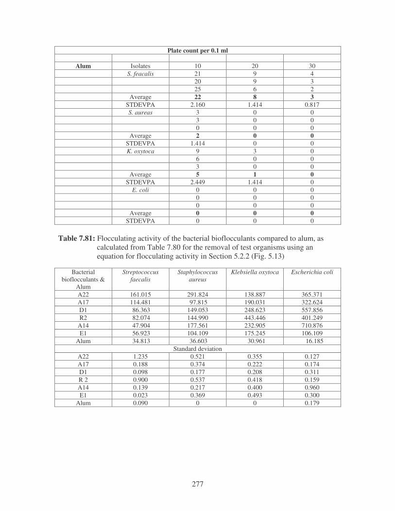
277
Plate count per 0.1 ml
Alum Isolates 10 20 30 S. feacalis 21 9 4 20 9 3 25 6 2 Average 22 8 3 STDEVPA 2.160 1.414 0.817 S. aureas 3 0 0 3 0 0 0 0 0 Average 2 0 0 STDEVPA 1.414 0 0 K. oxytoca 9 3 0 6 0 0 3 0 0 Average 5 1 0 STDEVPA 2.449 1.414 0 E. coli 0 0 0 0 0 0 0 0 0 Average 0 0 0 STDEVPA 0 0 0
Table 7.81: Flocculating activity of the bacterial bioflocculants compared to alum, as calculated from Table 7.80 for the removal of test organisms using an equation for flocculating activity in Section 5.2.2 (Fig. 5.13)
Bacterial bioflocculants &
Alum
Streptococcus faecalis
Staphylococcus aureus
Klebsiella oxytoca Escherichia coli
A22 161.015 291.824 138.887 365.371 A17 114.481 97.815 190.031 322.624 D1 86.363 149.053 248.623 557.856 R2 82.074 144.990 443.446 401.249
A14 47.904 177.561 232.905 710.876 E1 56.923 104.109 175.245 106.109
Alum 34.813 36.603 30.961 16.185 Standard deviation
A22 1.235 0.521 0.355 0.127 A17 0.188 0.374 0.222 0.174 D1 0.098 0.177 0.208 0.311 R 2 0.900 0.537 0.418 0.159 A14 0.139 0.217 0.400 0.960 E1 0.023 0.369 0.493 0.300
Alum 0.090 0 0 0.179
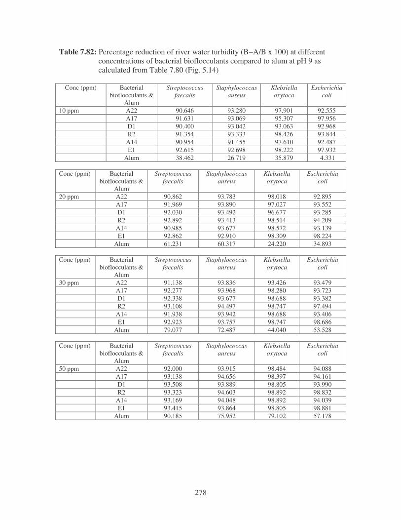
278
Table 7.82: Percentage reduction of river water turbidity (B−A/B x 100) at different concentrations of bacterial bioflocculants compared to alum at pH 9 as calculated from Table 7.80 (Fig. 5.14)
Conc (ppm) Bacterial bioflocculants &
Alum
Streptococcus faecalis
Staphylococcus aureus
Klebsiella oxytoca
Escherichia coli
10 ppm A22 90.646 93.280 97.901 92.555 A17 91.631 93.069 95.307 97.956 D1 90.400 93.042 93.063 92.968 R2 91.354 93.333 98.426 93.844 A14 90.954 91.455 97.610 92.487 E1 92.615 92.698 98.222 97.932 Alum 38.462 26.719 35.879 4.331 Conc (ppm) Bacterial
bioflocculants & Alum
Streptococcus faecalis
Staphylococcus aureus
Klebsiella oxytoca
Escherichia coli
20 ppm A22 90.862 93.783 98.018 92.895 A17 91.969 93.890 97.027 93.552 D1 92.030 93.492 96.677 93.285 R2 92.892 93.413 98.514 94.209 A14 90.985 93.677 98.572 93.139 E1 92.862 92.910 98.309 98.224 Alum 61.231 60.317 24.220 34.893 Conc (ppm) Bacterial
bioflocculants & Alum
Streptococcus faecalis
Staphylococcus aureus
Klebsiella oxytoca
Escherichia coli
30 ppm A22 91.138 93.836 93.426 93.479 A17 92.277 93.968 98.280 93.723 D1 92.338 93.677 98.688 93.382 R2 93.108 94.497 98.747 97.494 A14 91.938 93.942 98.688 93.406 E1 92.923 93.757 98.747 98.686 Alum 79.077 72.487 44.040 53.528 Conc (ppm) Bacterial
bioflocculants & Alum
Streptococcus faecalis
Staphylococcus aureus
Klebsiella oxytoca
Escherichia coli
50 ppm A22 92.000 93.915 98.484 94.088 A17 93.138 94.656 98.397 94.161 D1 93.508 93.889 98.805 93.990 R2 93.323 94.603 98.892 98.832 A14 93.169 94.048 98.892 94.039 E1 93.415 93.864 98.805 98.881 Alum 90.185 75.952 79.102 57.178
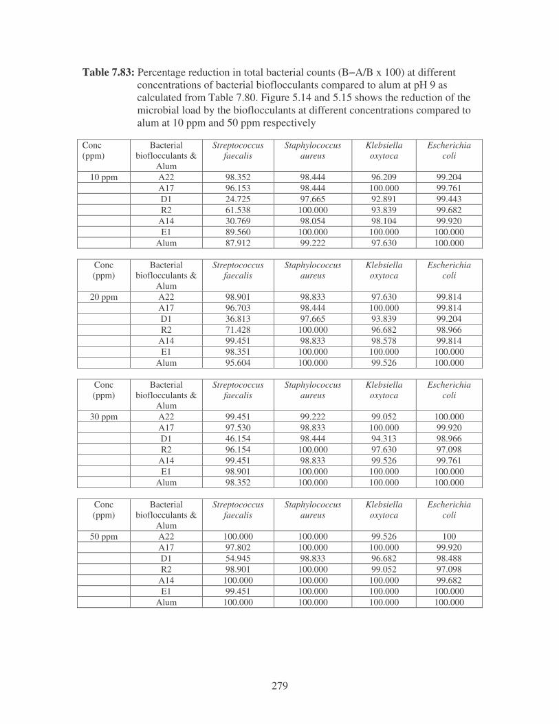
279
Table 7.83: Percentage reduction in total bacterial counts (B−A/B x 100) at different concentrations of bacterial bioflocculants compared to alum at pH 9 as calculated from Table 7.80. Figure 5.14 and 5.15 shows the reduction of the microbial load by the bioflocculants at different concentrations compared to alum at 10 ppm and 50 ppm respectively Conc (ppm)
Bacterial bioflocculants &
Alum
Streptococcus faecalis
Staphylococcus aureus
Klebsiella oxytoca
Escherichia coli
10 ppm A22 98.352 98.444 96.209 99.204 A17 96.153 98.444 100.000 99.761 D1 24.725 97.665 92.891 99.443 R2 61.538 100.000 93.839 99.682 A14 30.769 98.054 98.104 99.920 E1 89.560 100.000 100.000 100.000 Alum 87.912 99.222 97.630 100.000
Conc (ppm)
Bacterial bioflocculants &
Alum
Streptococcus faecalis
Staphylococcus aureus
Klebsiella oxytoca
Escherichia coli
20 ppm A22 98.901 98.833 97.630 99.814 A17 96.703 98.444 100.000 99.814 D1 36.813 97.665 93.839 99.204 R2 71.428 100.000 96.682 98.966 A14 99.451 98.833 98.578 99.814 E1 98.351 100.000 100.000 100.000 Alum 95.604 100.000 99.526 100.000
Conc (ppm)
Bacterial bioflocculants &
Alum
Streptococcus faecalis
Staphylococcus aureus
Klebsiella oxytoca
Escherichia coli
30 ppm A22 99.451 99.222 99.052 100.000 A17 97.530 98.833 100.000 99.920 D1 46.154 98.444 94.313 98.966 R2 96.154 100.000 97.630 97.098 A14 99.451 98.833 99.526 99.761 E1 98.901 100.000 100.000 100.000 Alum 98.352 100.000 100.000 100.000
Conc (ppm)
Bacterial bioflocculants &
Alum
Streptococcus faecalis
Staphylococcus aureus
Klebsiella oxytoca
Escherichia coli
50 ppm A22 100.000 100.000 99.526 100 A17 97.802 100.000 100.000 99.920 D1 54.945 98.833 96.682 98.488 R2 98.901 100.000 99.052 97.098 A14 100.000 100.000 100.000 99.682 E1 99.451 100.000 100.000 100.000 Alum 100.000 100.000 100.000 100.000