University of Rhode Island University of Rhode Island

DigitalCommons@URI DigitalCommons@URI

Open Access Master's Theses

1995

Application of an Electronic Fuel Injection System to a Single Application of an Electronic Fuel Injection System to a Single

Cylinder, Four Stroke Engine Cylinder, Four Stroke Engine

Glenn Michael Amber University of Rhode Island

Follow this and additional works at: https://digitalcommons.uri.edu/theses

Recommended Citation Recommended Citation Amber, Glenn Michael, "Application of an Electronic Fuel Injection System to a Single Cylinder, Four Stroke Engine" (1995). Open Access Master's Theses. Paper 1156. https://digitalcommons.uri.edu/theses/1156

This Thesis is brought to you for free and open access by DigitalCommons@URI. It has been accepted for inclusion in Open Access Master's Theses by an authorized administrator of DigitalCommons@URI. For more information, please contact digitalcommons@etal.uri.edu.

APPLICATION OF AN ELECTRONIC FUEL INJECTION SYSTEM

TO A SINGLE CYLINDER, FOUR-STROKE CYCLE

GASOLINE ENGINE

BY

GLENN MICHAEL AMBER

A THESIS SUBMITTED IN PARTIAL FULFILLMENT OF THE

REQUIREMENTS FOR THE DEGREE OF

MASTER OF SCIENCE

IN

MECHANICAL ENGINEERING AND APPLIED MECHANICS

UNIVERSITY OF RHODE ISLAND

1995

MASTER OF SCIENCE THESIS

OF

GLENN :MICHAEL AMBER

APPROVED:

Thesis Committee

:t:~ )1 /£i)2eJ DEAN OF THE GRADUATE SCHOOL

UNIVERSITY OF RHODE ISLAND

1995

ABSTRACT

One of the primary goals for any racing engine builder is to extract the maximum

amount of power possible from a given engine size. Achieving this goal is as valuable for

multiple cylinder, 500 or more cubic inch displacement automobile racing engines as it is

for single cylinder, small displacement go-cart racing engines. Fuel injection systems

have been manufactured that substantially increase the torque and power output of

multiple cylinder engines. An electronic fuel injection system was developed for a Briggs

& Stratton single cylinder gasoline engine that is similar to the type of engine used in

most go-cart racing divisions.

The engine was mounted to a dynamometer and the maximum wide open throttle

torque and power values were measured for the engine in the original carbureted

configuration. A different style carburetor with a variable air/fuel ratio was also tested.

The engine was then tested for maximum wide open throttle torque and power values

with the electronic fuel injection system installed. The first fuel injection tests were with

a fixed injector pulse width and an open loop control strategy. A closed loop strategy was

then developed and tested under a variety of fuel injection timing settings and lambda

sensor target values. Fuel injection resulted in torque and horsepower improvements at

all engine speeds, with approximately 20% torque and horsepower increase at top engine

test speed.

11

ACKNOWLEDGMENTS

I would like to express my sincere thanks to my professors, Dr. Philip Datseris

and Dr. Osama Ibrahim, for their insight and guidance throughout the research process.

Thanks are also extended to Dr. Peter Dewhurst for devoting the time to be a member of

my defense committee, and Dr. Winston Knight for chairing my defense committee.

Special thanks go to Jim Byrnes for his help with hardware and software interfacing

insights and to toolmaker Kevin Donovan for guidance with machining processes and

techniques. Thanks to Paul McGovern for the donation of components and insights. Very

special thanks go to Racin' Jason Miller for the donation of time, equipment and the

"speed secrets" that helped to make this project possible.

Special thanks also go out to my parents and family, whose support has been

constant throughout my life, and for the prayers and support of my friends.

111

TABLE OF CONTENTS

Abstract . . . . . . . . . . . . . . . . . . . . . . . . . . . . . . . . . . . . . . . . . . . . . . . . . . . . . . . . . . . . . . . . . . . . . . . . . . . . . . . . . . . . . . . . . . . . . . . . . . u

Acknowledgments .... ...... ...... ... ... ........ .... .. .. .... .... .... .......... .... .... .... .... . . 111

List of Tables . . . . . . . . . . . . . . . . . . . . . . . . . . . . . . . . . . . . . . . . . . . . . . . . . . . . . . . . . . . . . . . . . . . . . . . . . . . . . . . . . . . . . . . . . . . v1

List of Figures . . . . . . . . . . . . . . . . . . . . . . . . . . . . . . . . . . . . . . . . . . . . . . . . . . . . . . . . . . . . . . . . . . . . . . . . . . . . . . . . . . . . . . . . . vu

1 Introduction ......................................................................................... 1

1. 1 Objective .... ............. .... ..... .... .. ............ .... .. ... ... .... .. ..... .. ...... . ... . l

1.2 Background information .......... .. . . ... .. .... . .. .. .. . ... .. ...... .. . 1

1. 3 Theory of carburetor operation ... ...... ... .... ........ ... .. .... ..... .... 3

1.4 Theory of fuel injection operation . . . . ... .... ... . . . .. .. . ... .... ... ... 8

2 Description of test equipment and data acquisition system ............... 15

2.1 Engine ... ... .. ...... ... ... ....... .... ........... ... ..... .... ........ .... .... .. ..... . ..... 15

2.2 Dynamometer ..... .. ... ... ........... ....... .. ....... ..... .... ...... ........... .... ... . 17

2. 3 Data acquisition system . . . . . . . . . . . . . . . . . . . . . . . . . . . . . . . . . . . . . . . . .... ....... ... . 20

2. 3. 1 Torque measurement .. : . . . . . . . . . . . . . . . . . . . . . . . . . . . . . . . . . . . . . . . . . . . . . 22

2.3 .2 Engine speed measurement . . . . . . . . . . . . . . ... .. ... . ... . ...... 26

2.3.3 Exhaust oxygen measurement ... .......... ...... ......... .... .. 29

2.3.4 Temperature measurement .... ........ .... .... .... ..... . ... 29

2.3.5 Fuel injection timing .. ...... .............. ........ ...... ............ 31

2.4 Error Analysis ........ .... ... .. .. .... ........... ......... .... .... ..... ...... .. ... ... ... 33

3 Fuel injection system ........................................................................... 33

3.1 Hardware selection .... ...... .... ... ........... ... ..... ..... ..... .... .............. .. 33

IV

3 .2 Software selection . . . . . . . . . . . . . . . . . . . . . . . . . . . . . . . . . .. ..... ... ..... ........ .. .. .. 3 8

4 Comparisons and conclusions ............................................................ 42

4 .1 Flo-jet versus Pulsa-jet carburetor comparison .... ....... ... ... .. . .42

4.2 Constant pulse width fuel injection .. ..... ... .. .... ... .. .... . .... ... 54

4.3 Closed-loop fuel injection 65

4 .3. l 106° injection timing, varied lambda sensor target 65

4 .3.2 Injection timing optimization . 73

4 .3.3 93° injection timing, varied lambda sensor target ... 82

4.4 Fuel injection vs. carburetor comparison . . .. . .. . . ... . .. .. .. . ... . . .. . . . 89

4.5 Conclusions .. ... ..... .. . . . ... ......... .... ... ........ .... .. .. ... .. ... . 95

4 .6 Suggestions for further research . . . ... . . . ..... ...... ............. .. 96

References ................................................................................................ 99

Bibliography ............................................................................................ 100

v

4.1

4.2

LIST OF TABLES

Torque data, carburetors . . . . . . . . . . . . . . . . . . . . . . . . . . . . . . . . . . . . . . . . . . . . . . . . . . . . .. 44

Horsepower data, carburetors ... ........ ...... .... ........ .... .... ...... .. .. .. 45

4.3 Torque data, constant pulse width fuel injection .. ... .. ...... ... .... ...... .. 55

4.4

45

4.6

4.7

4.8

4.9

4.10

4.11

4.12

Horsepower data, constant pulse width fuel injection . . . . . . . . . . . . 55

Torque data, 106° fuel injection ... .... ... ..... ... .... ..... ..... .... ........ . ...... 66

Horsepower data, 106° fuel injection . . . . . . .. . . .. . .. .. .. . . . . . . . . ... ...... .. .... . 66

Torque data, variable fuel injection timing . .... ....... ........ .... ..... ..... .. 74

Horsepower data, variable fuel injection timing ...... .. .... .. .. .... . .... 75

Torque data, 93° fuel injection

Horsepower data, 93° fuel injection

............... .. ..... ........... .... .. .... .. 82

...... . .. .. ... .. ........ 82

Torque data, carburetor and fuel injection ... .. ..... .. ..... .. .. ........ ... ... .. 89

Horsepower data, carburetor and fuel injection ... .... ......... ... ... .... ... . 90

VI

1.1

1.2

1.3

1.4

1.5

1.6

2.1

2.2

2.3

2.4

2.5

2.6

3.1

LIST OF FIGURES

Schematic of carburetor with venturi . . . . . .... ... ........ ... .. ..... . .. ... 4

Pulsa-jet carburetor . . . .. . . . . . . ...... ... ..... ........ ... ........ ..... ... .. .. .. ... ... 5

Flo-jet carburetor ... ... ........ . ..... .... ............. ....... .... ........ .. ... . ... .. 6

Fuel injection overview ......... . . ... 10

Fuel injector cross-section . . . . . . . . . . . . . . . . . . . . . . . . . . . . . . . . . .. . . . . . . 11

Lambda sensor cross-section . . . . . . . . . . . . . . . . ..... .. .. .. ..... .... .. .. .. . 12

Engine and dynamometer overview .. . . .. . . .. . . .. . . .. . . . . . . . . . .. 17

Dynamometer rotor and stator . . .. . .. .. . . . . . . . . . . . . . . . . . . . . . . ....... ... . . 18

Belt drive system and load cell . . . . .. ... ... .... .. ...... ..... .. .... ...... .... . ... 19

Pressure transducer/load cell calibration graph ... ... ... .. .. ..... ... ... . .. 25

Tachometer generator calibration graph .. . .. .. .... .. ... .. ...... .. ... ... .. 28

Digital pickup and timing wheel . .. . .. . .. . . .. .... . ............ .. .... ... .. 31

Fuel injection schematic .... ........ . .............. .. .. ........ ...... .. .... . . . . 33

3 .2 Bosch fuel pump .. ·. ...... ............ .. ... .. .... ... ... . . . . . . . . . . . . . . . . . . . . . . . . . .. 34

3. 3 Bosch fuel pressure regulator ... ... : . . . .. . .. . . . .. . . .. . . . . . . . . .. .. . .. . . . .. . . .. . . .. . . . 3 6

3.4 Fuel injector and manifold .. ....... .. ... .. .. .. .... .. ..... ..... .. ... ... ........ ...... .. 37

3. 5 Lambda sensor graph .... .. .. ....... .. ...... ......... .. .. .... ... .... .. .. .. .... .. .... ..... 40

4. 1 Torque and horsepower graphs, pulsa-jet carburetor ... .. .. .. .... .... ..... 48

4.2 Torque and horsepower graphs, pulsa-jet carburetor .... .... .. .. .... ... ... 49

4.3 Torque and horsepower graphs, factory' s curves .... .. ...... ... ... ..... ..... 50

Vll

4.4 Torque and horsepower graphs, flo-jet carburetor .. ........... .. .. .. ... . 51

4.5 Torque and horsepower graphs, flo-jet carburetor ... .. .... ... ....... ... .. 52

4.6 Torque and horsepower graphs, flo-jet carburetor ... ... ...... . . 53

4.7 Torque and horsepower graphs, 2.5 ms constant injection .. .... ... .. .. . 57

4.8 Torque and horsepower graphs, 3 ms constant injection .. ... .. ... ... .. 58

4.9

4.10

4.11

Torque and horsepower graphs, 3 5 ms constant injection ... ... .... . .. 59

Torque and horsepower graphs, 4 ms constant injection .... ... .... .. . 60

Torque and horsepower graphs, 5 ms constant injection .... ..... .... ... 61

4.12 Torque and horsepower graphs, 5 5 ms constant injection .. .... 62

4.13

4.14

4.15

Torque and horsepower graphs, 6 ms constant injection ... .. .. ..... ... 63

Torque and horsepower graphs, 7 ms constant injection .... .... .. . ... 64

Torque and horsepower graphs, 0.85 lambda target, 106° .. ..... .... .. 68

4.16 Torque and horsepower graphs, 0.88 lambda target, 106° ·· ··· 69

4.17

4.18

Torque and horsepower graphs, 0.91 lambda target, 106° .. ... ....... . 70

Torque and horsepower graphs, 0.92-lambda target, 106° ...... ..... .. 71

4.19 Torque and horsepower graphs, 0.95 lambda target, 106°

4.20 Torque and horsepower graphs, 0:91 lambda target, 71°

4.21 Torque and horsepower graphs, 0.91 lambda target, 83°

.. 72

..... 77

.. 78

4. 22 Torque and horsepower graphs, 0. 91 lambda target, 93 ° . . . . . . . . . . . . . . . 79

4.23 Torque and horsepower graphs, 0.91 lambda target, 106° .. .. ... ... .... 80

4.24 Torque and horsepower graphs, 0.91 lambda target, 122° ....... ... .... 81

4.25 Torque and horsepower graphs, 0.85 lambda target, 93° .. ..... ....... .. 84

Vlll

4.26 Torque and horsepower graphs, 0.88 lambda target, 93° ...... ....... . 85

4.27 Torque and horsepower graphs, 0.91 lambda target, 93° .... .. ..... ..... 86

4.28 Torque and horsepower graphs, 0.92 lambda target, 93° .......... ..... . 87

4.29 Torque and horsepower graphs, 0.98 lambda target, 93° .......... ...... 88

4.30 Torque and horsepower graphs, pulsa-jet carburetor .... ......... ..... . 92

4.31 Torque and horsepower graphs, 0.88 lambda target, 93° . . . ... . 93

4.32 Torque and horsepower graphs, composite target, 93° . ........ ...... .. 94

lX

CHAPTER 1 : INTRODUCTION

l . 1 OBJECTIVES

The overall intent of this research was to demonstrate that a fuel injected engine

would produce more torque and horsepower than the same engine with a carburetor. The

engine was first tested for full throttle torque and horsepower production with the original

carburetor induction system in place. The only modification to the engine for this

segment of testing was the removal of the air filter assembly because the design of a

comparable air filter assembly for the fuel injection system was not an objective of this

experiment. The engine was then retrofitted with a custom designed fuel injection system,

while keeping the remainder of the engine unmodified. The fuel injected engine was then

subjected to the same series of tests as the carbureted engine. The results of the two

configurations were compared and analyzed.

1.2 BACKGROUND INFORMATION

Single cylinder gasoline engines are very common in the world today. They can

be found on a wide variety of power equipment including lawnmowers, generators,

garden tractors, rototillers, water pumps, weed wackers, and even on special applications

like racing go-carts and miniature drag racing cars. One of the primary design goals for

any of these pieces of equipment is to get the maximum possible torque and power output

from the smallest engine, thus making the powered equipment work better and faster, be

more portable and be easier to operate. In the special realm of high performance

1

applications like go-cart racing, drag racing and tractor pulling, the top priority for an

engine builder is to develop as much torque and power as possible from a particular

engine configuration. The optimum torque production for a specific application is not

always the maximum peak torque. For certain applications like generators and water

pumps, the engine speed is kept constant, so maximizing torque at that one operating

speed is very important. Since the engine is not run at any other speeds, the torque

produced at those speeds is irrelevant. In racing applications, the engine is cycled

throughout its range of operation so maximizing the torque across the whole RPM range

is much more important than having a high torque peak at one engine speed. Other

considerations like efficiency, economy, reliability, emissions production and cost play a

vastly diminished role in the development of engines for these special applications.

High performance, multiple cylinder automobile racing engines have been

successfully using fuel injection systems for well over 40 years. [1] In addition, the vast

majority of production automobiles sold in the United States in the last 10 years have

incorporated electronic fuel injection systems. Fuel injected engines perform better than

carbureted engines in almost all performance areas. [2] Technological advancements have

allowed designers to make electronic fuel injection systems that address the additional

design considerations like cost, efficiency and emissions that high performance

applications ignore. With many years of extensive research and development, electronic

fuel injection systems have been developed that are efficient, clean burning, reliable and

cost effective enough to sell to the general public in production vehicles.

2

Jn searching for performance improvements for one type of engine, it is common

practice to look at improvements that have been successful on other types of engines.

Since automobile manufacturers have well funded research and development programs,

many of the innovations in internal combustion engine technology are developed there,

and are adapted to other applications later. Fuel injection systems have proven to be

successfully used on automobile engines, both for racing and production vehicles. The

challenge was to broaden the scope of fuel injection technology and adapt it to a different

type of engine -- a single cylinder, four-stroke cycle Briggs and Stratton gasoline engine.

1.3 THEORY OF CARBURETOR OPERATION

The purpose of an induction system on an internal combustion gasoline engine is

to deliver a mixture of fuel and air which is to be drawn into the cylinder and burned. The

proportion of the amount of air to the amount of fuel is very important for proper engine

performance. This proportion is called air/fuel ratio. Since a typical engine has to run at a

variety of different speeds, loads, temperatures, and conditions, the induction system

must be able to adapt accordingly. The most common induction system used on small

engines is a carburetor. Although there are many different types of carburetors designed

with varying levels of complexity, they all use the same basic principle of operation. Air

is drawn into the engine through the main opening in the carburetor. This main passage

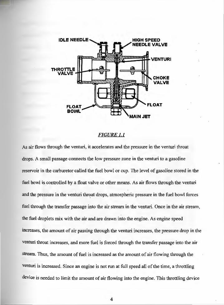
contains a venturi as demonstrated in Figure 1.1.

3

IDLE NEEDLE

FLOAT BOWL

FIGURE 1.1

HIGH SPEED NEEDLE VALVE

CHOKE VALVE

As air flows through the venturi, it accelerates and the pressure in the venturi throat

drops. A small passage connects the low pressure zone in the venturi to a gasoline

reservoir in the carburetor called the fuel bowl or cup. The level of gasoline stored in the

fuel bowl is controlled by a float valve or other means. As air flows through the venturi

and the pressure in the venturi thr~at drops, atmospheric pressure in the fuel bowl forces

fuel through the transfer passage into the air stream in the venturi. Once in the air stream,

the fuel droplets mix with the air and are drawn into the engine. As engine speed

increases, the amount of air passing through the venturi increases, the pressure drop in the

venturi throat increases, and more fuel is forced through the transfer passage into the air

stream. Thus, the amount of fuel is increased as the amount of air flowing through the

venturi is increased. Since an engine is not run at full speed all of the time, a throttling

device is needed to limit the amount of air flowing into the engine. This throttling device

4

consists of a flat metal disc called a throttle plate mounted on a shaft. In the wide open

position, the throttle plate offers almost no restriction to the flow of air through the

carburetor. As the shaft is rotated, the throttle plate restricts the flow of air into the

engine. As the airflow is reduced, the engine speed and power produced are also reduced.

At idle speed, the throttle valve is almost fully closed and airflow through the venturi is

minimized. At idle, the pressure drop in the venturi is so small at the minimum air flow

that there is no fuel drawn into the engine. A separate small fuel passage, called the idle

circuit, supplies fuel at low engine speeds. The amount of fuel that flows through these

passages in the carburetor is precisely metered either by an adjustable needle valve or by

an orifice. [3]

FIGUREJ.2

The carburetor used for part of this experiment is a Briggs & Stratton pulsa-jet carburetor,

Figure 1.2. The carburetor is mounted directly on top of the fuel tank. The pulsa-jet

5

carburetor has an integrated fuel pump that draws fuel up from the main portion of the

fuel tank and fills a reservoir located under the venturi. A constant fuel level in the

reservoir is maintained by allowing excess fuel to drain back into the main part of the fuel

tank. The fuel tube between the venturi and the fuel reservoir contains an orifice that

meters the amount of fuel that flows into the engine. This orifice, or main jet, controls the

high speed air to fuel ratio and is not adjustable. The idle circuit is adjustable by means of

a needle valve that is externally adjustable. The remainder of the pulsa-jet carburetor is

consistent with the general carburetor description given above.

FIGURE 1.3

The other carburetor used for a portion of this experiment is a Briggs & Stratton

flo-jet carburetor, Figure 1.3. The flo-jet is a gravity feed, float type carburetor. The fuel

tank is mounted at a height above the carburetor. A fuel line supplies fuel to the inlet of

the carburetor. Fuel flows into a reservoir in the carburetor called a fuel bowl. A constant

fuel level in the bowl is maintained by a float valve as described in the paragraph above.

6

Both the high and low speed fuel passages on the flo-jet carburetor contain adjustable

needle valves.

Carburetors have a number of drawbacks that limit their usefulness, especially for

high performance applications. Because the amount of fuel flow is dependent on the air

flow through the venturi, changes in fuel flow happen only after there have been changes

in air flow. This means that a carburetor can only react to changes in air flow that have

already occurred. This is a problem is when the throttle is opened quickly. The airflow

through the venturi increases immediately, but the corresponding fuel flow does not

increase immediately. This causes the engine to lean out and misfire or stall completely.

In an application like circle track racing, where the driver is constantly decelerating and

then quickly accelerating in and out of turns, this throttle lag can be even more of a

problem. Automobile carburetors deal with this problem by installing accelerator pumps,

which squirt extra fuel into the venturi whenever the throttle is opened. Neither the flo-jet

nor pulsa-jet carburetors have an accelerator pump.

The venturi, which is critical for a carburetor to function, limits the engine' s

performance capability. For the venturi in the carburetor to work, especially at low engine

speeds, it has to be small enough to restrict air flow and cause a pressure drop. This

restriction limits the amount of air that can flow through the carburetor at high engine

speeds, and therefore reduces high speed torque and power production. If the venturi is

sized larger for maximum top speed air flow, the low speed performance will suffer.

7

1..4 THEORY OF FUEL INJECTION OPERATION

Fuel injection performs the same task as a carburetor -- to mix fuel and air in the

correct proportion for the engine to perform well. While the end result is the same, the

method of achieving this result is quite different. Fuel injection systems do not rely on a

pressure drop in a venturi like a carburetor does. Injection systems pressurize the fuel and

force it through a special nozzle. The nozzle atomizes the fuel into a fine mist which

mixes with the air being drawn into the engine during the intake stroke.

Mechanical fuel injection systems were offered on a limited number of domestic

production vehicles starting in 1957. Chrysler offered the first electronic fuel injection

system in 1958. The system, called the "Electrojector," was very expensive for the time

period ($400-$500) and its sales were minimal as less than 100 vehicles were sold. This

first electronic fuel injection system was manufactured by Bendix, who soon sold the

manufacturing rights to the Bosch company. The first Bosch electronic fuel injection

equipped production car was a 1968 Volkswagen. [4]

In the early 1970's, concern for the environment and increasing dependence on

foreign oil supplies spurred the government to enact legislation controlling the fuel

economy and pollution levels of automobiles. As carburetor systems became increasingly

more complex and expensive, manufacturers realized that carburetors would be hard

pressed to meet the future government standards. Fortunately, work in the electronics

field was producing inexpensive and reliable solid state components. These advances

were applied to the electronic fuel injection systems. The resulting systems were much

more dependable and less expensive. In 1975, an electronic fuel injection system

8

eared in a domestically produced Cadillac Seville. Now virtually all of the cars sold reapp

in America are equipped with electronic fuel injection systems. [5]

The first fuel injection systems were mechanical. Mechanical fuel injection

systems use fuel injectors that only open when the pressure in their supply lines exceeds a

certain value. A mechanical fuel metering system pressurizes each injector in a specific

timing sequence. As the fuel pressure in the fuel lines exceeds the release value for the

fuel injector, the fuel is sprayed into the intake manifold or port. As soon as the fuel

metering system cuts off fuel delivery to an injector, it closes. The fuel injectors for

mechanical fuel injection systems are simpler than electronic fuel injectors, but

mechanical fuel injection is less versatile. Mechanical fuel injection delivery systems are

very complicated to design and optimize. They require complex arrays of cams and rotors

to vary the fuel delivery for different engine loads and throttle positions. Once a

mechanically fuel injected engine is built and running, there is very little that can be done

to optimize the amount of fuel delivered, or to change the timing at which it is delivered,

without stopping the engine and making mechanical adjustments.[6]

In contrast, electronic fuel injection systems are continually optimized as the

engine is running. As the operating conditions or engine load changes, sensors

relay information to the electronic control unit, which compensates by varying the

amount of fuel injected.

9

"O" Ring

FIGURE 1.4

Virtually all current electronic fuel injection systems consist of the same basic

components. A fuel pump, fuel pressure regulator, fuel injector or injectors, electronic

control unit, and a series of sensors are all incorporated by typical electronic fuel

injection systems, as in Figure 1.4. The fuel pump is driven by a 12 volt electric motor. It

supplies a flow of high pressure gasoline to the fuel system. The fuel pressure regulator

maintains the fuel supply at a predetermined pressure by allowing excess fuel to return to

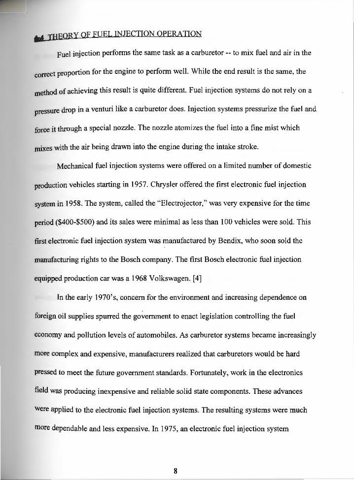
the fuel tank. The fuel injector is an electric solenoid valve, Figure 1.5. The injector is

either open or closed. When no voltage is applied to its terminals, it is closed and no fuel

will flow through it. When voltage is applied to it, the injector will open fully, and a

steady flow of fuel will pass through it. The end of the fuel injector is equipped with a

special nozzle which atomizes the fuel into a cone-shaped spray pattern. The fuel flow

rate is determined by two factors. The first factor is the size of the injector nozzle. The

larger the nozzle, the more fuel flow it will allow. The second factor is the fuel pressure

10

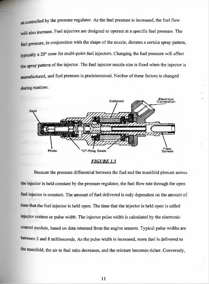
as controlled by the pressure regulator. As the fuel pressure is increased, the fuel flow

will also increase. Fuel injectors are designed to operate at a specific fuel pressure. The

fuel pressure, in conjunction with the shape of the nozzle, dictates a certain spray pattern,

typically a 20° cone for multi-point fuel injectors. Changing the fuel pressure will affect

the spray pattern of the injector. The fuel injector nozzle size is fixed when the injector is

manufactured, and fuel pressure is predetermined. Neither of these factors is changed

during runtime.

Pintle "O"-Ring Seals

FIGUREJ.5

Electrical Connection

Because the pressure differential between the fuel and the manifold plenum across

the injector is held constant by the· pressure regulator, the fuel flow rate through the open

fuel injector is constant. The amount of fuel delivered is only dependent on the amount of

time that the fuel injector is held open. The time that the injector is held open is called

injector ontime or pulse width. The injector pulse width is calculated by the electronic

control module, based on data returned from the engine sensors. Typical pulse widths are

between 2 and 8 milliseconds. As the pulse width is increased, more fuel is delivered to

the manifold, the air to fuel ratio decreases, and the mixture becomes richer. Conversely, (

11

when the pulse width is shortened, the air to fuel ratio is increased, and the mixture

becomes leaner.

There are two common types of fuel injection that use electronically controlled

injectors. One type is called throttle body or central fuel injection. This system uses one

or two large fuel injectors located in what amounts to a carburetor-type body. The

injector(s) spray fuel into an essentially conventional intake manifold. Throttle body

injection provides more accurate fuel metering than a conventional carburetor system,

and allows for feedback control of the air to fuel ratio.

The second type of injection is electronically timed injection, commonly called

multi-point, multi-port, or sequential fuel injection. Multi-point fuel injection systems use

one small fuel injector for each cylinder. Each injector is positioned to spray directly at an

intake valve, and will spray at a specified time relative to the opening of the valve. This

specified time is called the injection timing and is measured in degrees of crankshaft

rotation before the intake valve begins to open.

Protective Outer

S'i°ve

FIGURE 1.6

12

Contact Cover

The most important sensor for feedback control of the electronic fuel injection system is

the exhaust oxygen sensor or Lambda sensor, Figure 1.6. The oxygen sensor is threaded

into the exhaust manifold of the engine, typically ahead of the catalytic converter in an

automotive application. The sensor consists of a thimble-shaped Zr02 ceramic sensing

element. The sensor is exposed to the exhaust stream on its outside and atmospheric air

on its inside. The Zr02 electrode produces a small voltage in proportion to the ratio of the

amount of oxygen in the exhaust stream to the amount of oxygen in the ambient air.

When the amount of oxygen in the exhaust increases (the air to fuel ratio gets higher; the

engine runs leaner) the voltage produced by the Lambda sensor decreases. When the air

to fuel ratio decreases (the engine runs richer) the amount of exhaust oxygen decreases,

and the voltage produced by the Lambda sensor increases. The range for the Lambda

sensor is 0 to 1 volts, 0 being an extremely lean mixture and 1 being an extremely rich

mixture. An output of 0.5 volts indicates the ideal stoichiometric air to fuel ratio of

14.7:1. The Lambda sensor does not function until it reaches an operating temperature of

greater than 900°C, so an engine must warm up under open loop control before the sensor

will feed back the signal required to close the control loop. [7] The oxygen sensor

voltage is essential to the feedback control system. of the electronic fuel injection system.

If the engine runs lean, the electronic control unit increases the injection pulse width,

making the mixture richer. Conversely, if the engine runs too rich, the control unit

shortens the ontime of the fuel injectors to lean the mixture.

Production automotive fuel injection systems incorporate a number of different

sensors to more accurately control and anticipate changes in the fuel delivery

13

·rements These sensors help to maintain performance and economy under a very requ1 ·

wide range of operating conditions. Most electronic fuel injection systems incorporate a

variety of combinations of these auxiliary sensors for optimum operation. Some injection

systems measure the amount of air entering the engine as a variable to calculate fuel

requirements. The amount of incoming air can be measured by an air mass sensor or an

air flow sensor. Engine throttle plate position can be measured using a special

potentiometer called a throttle position sensor. The amount of engine vacuum (used as a

measure of engine load) can be measured with a manifold absolute pressure (MAP)

sensor. Engine speed can be measured with a tachometer. Incoming air temperature,

cylinder head temperature, engine coolant temperature, atmospheric pressure, vehicle

speed, and battery voltage can also be measured and used to adjust the injection pulse

width to optimize vehicle performance or economy. [8] A list of the specific sensors

chosen for the single cylinder electronic fuel injection system are given in Chapter 2.3.

14

QIAPTER 2 : TEST EQUIPMENT AND DAT A ACQUISITION SYSTEM

Z..l TEST ENGINE

The test engine that was selected to be fitted with the experimental electronic fuel

injection system was a Briggs & Stratton gasoline engine model number 130232 4036-01

92031307, Figure 2.1. The 130232 series Briggs & Stratton engine has a vertical

aluminum cylinder bore with a diameter of 2.56 inches, and has a crankshaft stroke of

2.44 inches. This bore and stroke combination yields a displacement of 12.57 cubic

inches. The engine has a horizontal crankshaft arrangement and is equipped with a

mechanical flyweight governor. The function of the governor is to maintain a constant

engine rotational speed under varying engine load conditions. Since all of the tests for

this research were performed under full load, wide open throttle conditions, the governor

was only utilized as a safety feature to prevent engine damage from accidental,

uncontrolled overspeeding. The factory horsepower rating of 5 HP is at 3600 RPM. Some

of the engine tests for the carburetor and injection sys.terns were performed up to the 3600

RPM maximum speed while others were performed up to a maximum speed of 4600 rpm.

The 4600 RPM was considered the maximum safe engine speed without performing

substantial engine modifications to permit safe higher RPM operation. The crankshaft is

supported in the engine block by ball bearings and the engine is started manually with a

rewind type starter. This engine model is originally manufactured with a 'pulsa-jet'

carburetor. The pulsa-jet carburetor is designed as an integral part of a the fuel tank. Refer

to Section 1.2 for complete details on the pulsa-jet carburetor.

15

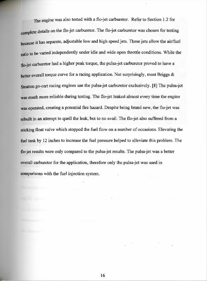
The engine was also tested with a flo-jet carburetor. Refer to Section 1.2 for

complete details on the flo-jet carburetor. The flo-jet carburetor was chosen for testing

because it has separate, adjustable low and high speed jets. These jets allow the air/fuel

ratio to be varied independently under idle and wide open throttle conditions. While the

flo-jet carburetor had a higher peak torque, the pulsa-jet carburetor proved to have a

better overall torque curve for a racing application. Not surprisingly, most Briggs &

Stratton go-cart racing engines use the pulsa-jet carburetor exclusively. [8] The pulsa-jet

was much more reliable during testing. The flo-jet leaked almost every time the engine

was operated, creating a potential fire hazard. Despite being brand new, the flo-jet was

rebuilt in an attempt to quell the leak, but to no avail. The flo-jet also suffered from a

sticking float valve which stopped the fuel flow on a number of occasions. Elevating the

fuel tank by 12 inches to increase the fuel pressure helped to alleviate this problem. The

flo-jet results were only compared to the pulsa-jet results. The pulsa-jet was a better

overall carburetor for the application, therefore only the pulsa-jet was used in

comparisons with the fuel injection system.

16

FIGURE2.1

2.2 DYNAMOMETER

The dynamometer utilized for this research was a Go-Power Systems model DY-7D

waterbrake dynamometer, Figure 2. 1. The most important part of a waterbrake

dynamometer is the absorption unit. The absorption unit converts the rotational torque of

the engine to a measurable linear force. The absorption unit consists of a finned rotor

rigidly attached to a shaft. The rotor is assembled· inside of a stator housing that has fins

on its inside surface. The rotor is supported inside of the stator by ball bearings, and is

connected to the test engine by a flexible coupler, Figure 2.2. A control valve regulates

the amount of water that is pumped into the absorption unit or stator housing.

17

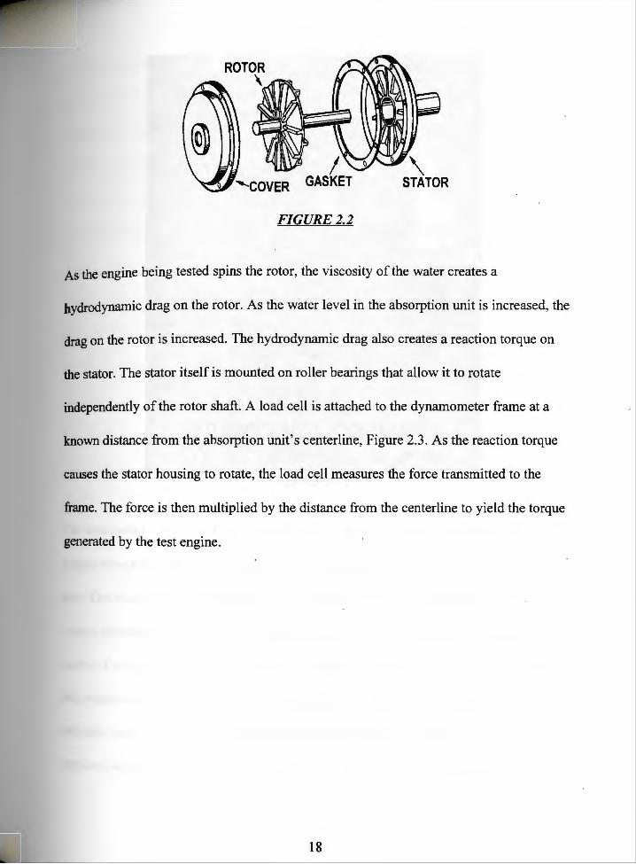
FIGURE2.2

As the engine being tested spins the rotor, the viscosity of the water creates a

hydrodynamic drag on the rotor. As the water level in the absorption unit is increased, the

drag on the rotor is increased. The hydrodynamic drag also creates a reaction torque on

the stator. The stator itself is mounted on roller bearings that allow it to rotate

independently of the rotor shaft. A load cell is attached to the dynamometer frame at a

known distance from the absorption unit's centerline, Figure 2.3. As the reaction torque

causes the stator housing to rotate, the load cell measures the force transmitted to the

frame. The force is then multiplied by the distance from the centerline to yield the torque

generated by the test engine.

18

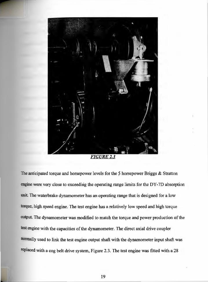
FIGURE2.3

The anticipated torque and horsepower levels for the 5 horsepower Briggs & Stratton

engine were very close to exceedirig the operating range limits for the DY-7D absorption

unit. The waterbrake dynamometer has an operating range that is designed for a low

torque, high speed engine. The test engine has a relatively low speed and high torque

output. The dynamometer was modified to match the torque and power production of the

test engine with the capacities of the dynamometer. The direct axial drive coupler

nonnally used to link the test engine output shaft with the dynamometer input shaft was

replaced with a cog belt drive system, Figure 2.3. The test engine was fitted with a 28

19

th 112 inch pitch pulley. The dynamometer input shaft was fitted with a 14 tooth too ,

pulley with the same pitch. The dynamometer stator housing was elevated on a specially

designed platform that aligned the two pulleys directly above one another. A 314 inch

wide, 112 inch pitch, fiberglass-reinforced timing belt was used to connect the two pulleys

with no slippage and very high mechanical efficiency. [9] The belt drive system doubles

the output speed of the engine into the dynamometer. Since the power transfer must

remain constant (excluding any frictional or other losses) the torque at the dynamometer

input shaft must be one half of the torque at the engine output shaft. The speed doubling

belt drive system conditions the operating range of the engine output to match the

operating range of the dynamometer. Since the experiment is designed to be a comparison

between a carburetor and a fuel injection system on the exact same test engine and

dynamometer apparatus, frictional losses and other losses that cause the torque and

horsepower measurements to vary from their actual values are negligible because they act

on both test variations equally.

2.3 DATA ACQUISITION SYSTEM

As will be detailed in the following sections, all of the analog data acquisition

devices were replaced or upgraded to digital devices. These upgrades improve the

accuracy of the results in a number of ways. First, the error associated with a human

being reading analog gauges is eliminated. In addition, the amount of time required

between various data readings to record results is eliminated if a computer is used to

sample the results. The computer system needed a special interface to measure voltage

20

. 1 This interface was a Real Time Devices model AD 1100 analog to digital s1gna s.

rter board Four analog to digital conversion channels were used to measure engine conve ·

Ue Speed exhaust oxygen content, and temperature. One of the parallel output ports torq , '

on the board was used for binary outputs to control the engine kill relay, the fuel pump

relay and the fuel injector itself. An analog to digital converter board can take consecutive

readings in a matter of microseconds. This speed improvement over hand documented

data measurement helps to assure that the torque data and the corresponding speed data

are correct. The speed of a reciprocating internal combustion engine is always fluctuating

because the engine produces power only one out of four strokes. Since four strokes

corresponds to two revolutions, the engine accelerates one half of one rotation every two

rotations. The engine is accelerating during this power stroke, as the air/fuel mixture is

burning. The inertia of the moving components in the engine does work for the remaining

portion of the cycle, which is to intake in the air/fuel mixture, compress it, and exhaust it

from the cylinder after it is burned. The engine is decelerating for these other 3 strokes or

1-112 rotations of the crankshaft. Thus, the engine is never truly running at a constant

speed. This speed variation leads to potential measurement difficulty. The shorter the

interval between the time that the torque is measured and the time that the speed is

measured, the more accurate the power calculation will be. If the data must be read and

recorded by hand, the two values may be 10 or more seconds apart. At 3600 RPM, 10

seconds equals 600 revolutions or 300 complete acceleration/deceleration cycles. Even if

an analog to digital converter board takes readings at 1 millisecond intervals (the Real

21

. Devices' ADl 100 board takes readings on the order of 10 times that fast), torque Time

and speed readings will be measured during the same revolution. [1 O]

ZJ.l Torque Measurement

The dynamometer was originally manufactured with simple analog gauges for

data acquisition. The engine torque, for example, was measured by a hydraulic pressure

gauge. The load cell (as mentioned in section 2.2 and shown in Figure 2.3) is fixed to the

dynamometer frame on one end and to the movable stator housing on the other end. The

toad cell contains a piston and rolling diaphragm which seals a chamber filled with

silicon fluid. As the hydrodynamic drag from the rotor applies torque to the stator, the

stator transmits a reaction force to the load cell. The pressure in the silicon fluid under the

piston increases in direct proportion to the torque on the stator. The fluid pressure was

measured by a gauge mounted on the dynamometer frame. As calibrated from the factory,

the gauge read foot-pounds of torque.

The system functioned adequately as designed for basic laboratory experiments

and for teaching the fundamentals of internal combustion engine design and testing. For

precision research, more accurate results were needed. The analog gauges supplied with

the dynamometer have many drawbacks. First, human error in reading the gauges causes

inaccurate readings. As detailed in the previous section, power transfer to the output shaft

is not smooth. This unsteady nature of a reciprocating engine causes pressure highs and

lows in the silicon fluid in the load cell, which causes needle flutter on an analog pressure

gauge. Since the needle flutters at an approximate frequency equal to the rotational

22

Cy of the engine, the error associated with reading the gauge can be substantial. [requen

tl'fy this problem, a pressure transducer was installed in the pressure line between To rec

the load cell and the torque gauge. The original equipment flexible nylon pressure lines

were replaced with rigid steel lines to reduce errors due to elastic expansion of the lines

under pressure. The pressure transducer is still subject to the same pressure fluctuations

that the analog gauge was, but the data acquisition program was able to take a number of

readings and average them to create each data point.

Since the effective area under the load cell diaphragm was not known, and the

manufacturer was unwilling to provide the information, the load cell and pressure

transducer had to be calibrated. By disassembling the dynamometer stator unit, the

perpendicular distance from the centerline of the stator body to the point of force

application on the load cell was measured to be 0.308 feet. This distance will later be

multiplied by the force measured at the load cell to calculate the torque applied to the

stator housing by the hydrodynamic drag. A special calibration fixture was designed and

built to hold the load cell after removing it from the rest of the dynamometer. All of the

air was bled from the fluid lines. A known mass was suspended from the end of the load

cell calibration fixture. Since the length from the fµlcrum point of the upper beam to the

force application point on the load cell was twice the distance from the fulcrum point to

the point from which the weights were hung, the effective force at the load cell was two

times the weight hung from the beam. The output from the pressure transducer was

measured with a digital volt-ohm meter. A number of known masses were hung from the

calibration fixture beam, and the corresponding data from the pressure transducer was

23

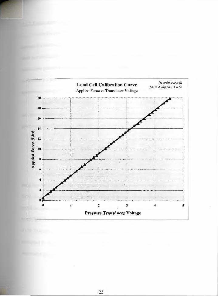
d d The data was tabulated on a spreadsheet and the results were plotted, Figure recor e ·

Z.4. As expected, the points on the force versus voltage plot were linear, and the equation

for the line was calculated. (equation 2.1) This equation allows the force on the load cell

in pounds to be calculated from the voltage output of the pressure transducer.

F load cell = 0.58 + 4.26 * ( V transducer - 4. 77) (equation 2.1)

When the equation is multiplied by the effective torque arm of the stator (0.308 ft) the

torque at the stator in foot-pounds can be calculated from the force on the load cell.

T stator = 0.308 * F load cell (equation 2.2)

Combining equations 2.1 and 2.2, then multiplying by two (the torque reduction due to

the cog belt drive) gives torque at the engine output shaft in foot-pounds as a function of

pressure transducer output voltage.

T engine = 0.36 + 2.62 * ( V tra~sducer - 4. 77) (equation 2.3)

24

-~ ~

20

Load Cell Calibration Curve Applied Force vs Transducer Voltage

I st order curve fit Lbs= 4.26(volts) + 0.58

e. 12 +-~~~~~+-~~~~~-t--~~---,~~-r-~~~~~-r-~~~~~4 QI

~ ~ 10+-~~~~~-i-~~~~~-i-~~~~~-r-~~~~~-r-~~~~~4

] 8 Q. -1-~~~~~-1-~~~~=--1-~~~~~+-~~~~~+-~~~~----l

c. <

0 2 3

Pressure Transducer Voltage

25

4 5

3 2 En<Jine speed measurement ~· __ ..

After the dynamometer stator housing was elevated to accommodate the belt drive

tern the mechanical shaft drive tachometer was no longer functional because the input sys ,

shaft was no longer collinear with the output shaft on the stator housing. An electric

tachometer generator was mounted on the front of the test engine. A tachometer generator

is essentially a permanent magnet electric motor that is forced to rotate. The tachometer

generates a voltage that is directly proportional to the speed of its input shaft.

Although the tachometer generator was supplied with a calibration equation, the

unit was calibrated again to help insure the accuracy of the results. The manufacturer' s

given equation of speed as a function of output voltage was:

RPM= 1000/ 7 * V tach (equation 2.4)

The analog to digital converter board that was used for these tests had a maximum

range limit of+ 10 volts de. At the anticipated absolute maximum engine speed of 5000

RPM, the tachometer would generate 35 volts. A voltage divider circuit was used to

match the operating ranges of the tachometer generator and the analog to digital converter

hoard. The resistors used in the voltage divide circuit had a measured division ratio of

4. 178. Therefore, all voltage readings measured by the analog to digital converter were

multiplied by the conversion factor of 4. 178 to get the actual voltage produced by the

tachometer generator.

26

The tachometer remained installed on the test engine for the calibration procedure.

A sirometer was used to measure the engine rpm, and a digital voltmeter was used to

measure the tachometer generator output from the voltage divider circuit. The data points

were curve fitted with a first order curve, and the equation of the curve was calculated.

{See figure 2.5} The new calibration curve for the tachometer generator varied slightly

from the manufacturers claimed curve. The equation for engine speed as a function of

tachometer generator voltage out of the voltage divider circuit was as follows:

RPM= 733.9 * v tach (equation 2.5)

27

Figure 2.5 I st order forced thru origin Tachometer Generator Calibration RPM= 733 9(VtachJ

Engine Speed vs Tach Voltage R2 = o.9981

------·-------- ----1 4000 1------~----+-----t-----t------t-----::~-~I

i

0 2 3 4 s 6

Tachometer Voltage

28

Exhaust oxygen content 2.J.3 --The primary feedback control variable for electronic fuel injection systems is the

en sensor voltage. For a complete description of oxygen sensor components and oxyg

[unction, refer to section 1.3. The oxygen sensor values were recorded for all engine tests,

including pulsa-jet and flo-jet carburetor tests that actually did not need to use the values

for feedback. Since the air to fuel ratio can have a dramatic effect on engine torque and

power production, the values were recorded for future reference. When the electronic fuel

injection system was tested in a closed loop form, the average values oxygen sensor

values from the carburetor data sets were used as target values for the feedback control

system. This ensured that increases in torque and power production were not due to

changes in air to fuel ratio.

2.3 .4 Temperature measurement

An engine temperature measurement was only required to determine that the

engine was at operating temperature and was ready to.go into closed loop control. The

temperature data could also be used as an integral part of the feedback control. Typical

fuel injection systems operate in an open loop with no feedback control when they are

cold. Once the engine has reached operating temperature, the computer control unit goes

into closed loop mode and gets feedback data from designated monitoring sensors. Since

this particular test did not require any more accurate temperature measurements than to

distinguish between a cold engine and a warm engine, sophisticated temperature

measurement technology was not required. A negative temperature coefficient thermistor

29

d for temperature measurements. A negative temperature coefficient thermistor is was use

. ble resistor. As the temperature of the thermistor increases, its electrical resistance avana

ases When assembled into a simple circuit with a fixed resistor to limit maximum decre ·

current level, the voltage across the thermistor will vary in inverse proportion to the

temperature of its surroundings.

The thermistor was mounted on the outlet vent of the air-cooling system of the

engine. At room temperature with the engine cold, the voltage drop across the thermistor

was approximately 4.5 volts. When the engine was run and attained operating

temperature, the airflow out of the vent would warm, and the voltage drop across the

~

thennistor was lower. At operating temperature with the engine idling with no

dynamometer load, the voltage drop across the thermistor was approximately 3.75 volts.

At the maximum operating temperature, which was full dynamometer load, wide open

throttle, low engine speed, the voltage drop across the thermistor was approximately 1.9

volts. A measured voltage oflower than 3.80 volts was considered a fully warmed up

engme.

30

FIGURE2.6

2.3.5 Fuel injection timin2

One additional sensor is needed to define the precise time at which the electronic

fuel injection system must inject fuel. This is appropriately called injection timing. Fuel

injection timing is typically measured in degrees of crankshaft rotation before the intake

valve begins to open. A digital magnetic pickup was used to set the injection timing for

the research engine, Figure 2.6. A digital magnetic pickup is a cylindrical shaped piece of

stainless steel with a magnetic tip. A non-ferrous rotor was mounted on the crankshaft of

the engine. The position of the rotor was held fixed by means of an Allen head set screw.

Loosening the Allen head screw allowed the rotor to be rotated relative to the crankshaft

31

h. ve the desired fuel injection timing. On the outer rim of the rotor is a small steel to ac ie

b The tab protrudes beyond the edge of the rotor by 0.055 inches. When the engine ta .

t S and the tab passes by the digital magnetic pickup, the pickup produces a rota e

conditioned step wave voltage signal. The digital magnetic pickup is wired into the

computer interrupt generator, which signals the computer that the reference point on the

rotor has just passed, and to begin the injection process.

2A ERROR ANALYSIS

The main source of error in an experiment of this type is typically due to

inaccuracies in the sensors and measuring equipment. If the object of this experiment was

to measure the torque and horsepower produced and compare the results to some other

experiment, then calibration of the sensors to international standards would be critical.

This experiment is designed as a comparison between two induction systems on the same

engine, measured on the same dynamometer, with the same controlled atmospheric

conditions. Errors in horsepower due to small fluctuations in atmospheric conditions were

less than ± 1 % . The error in the measurement of the load cell torque arm was

approximately± 0.14%. The error in the data from.the pressure transducer was

approximately ± 2.2%. The analog to digital converter produced approximately ± 0.25%

error. The tachometer assembly had an estimated total error of± 2.25%. The total error in

the horsepower measurements due to the sensors and measuring systems was

approximately± 4.9%. The estimated total error due to all listed factors was less than±

6%.

32

CHAPTER 3 : FUEL INJECTION SYSTEM

LOW PRESSURE -4----;+-..,.._-- FUEL RETURN

LINES

HIGH PRESSURE _,_ FUEL SUPPLY LINE

FUEL PRESSURE

/REGULATOR

FUEL INJECTOR----FUEL

,~f_t, /SPRAY , ... ... ~. <-.»~.: ~ ......

;~:· -. r.~~ .

FIGURE3.1

3.1 HARDWARE SELECTION AND DESIGN

Because there are very few electronic fuel injection systems in common use on

engines smaller than automobile engines, components appropriately sized for a single

cylinder engine were not readily available. Locally available automobile fuel injection

parts that were as close as possible or exceeded the requirements of the fuel injection

design were used. Most of the components are of larger capacity than a small engine

required but well suited for the test engine. Figure 3.1 shows a schematic of the fuel

injection system as it was applied to the Briggs & Stratton test engine.

The fuel pump was an externally (outside of the fuel tank) mounted Bosch part

number 0 580 463 005. The fuel pump is powered by a 12 volt direct current electric

motor. It will pump 30 gallons of gasoline per hour at free flow, and will produce up to

l lO psi pressure with the relief valve fully closed. It has three-5/16 inch outside diameter

33

fuel line fittings located on one end. The first fitting is the fuel supply to the fuel pump

and was connected to the shutoff valve on the bottom of the fuel tank by a low pressure

neoprene fuel line. This small section of fuel line also contained the fuel filter, so that all

fuel was filtered before it reached the pump or any of the other components. The second

fitting on the fuel pump was an return outlet from the pressure relief valve built into the

fuel pump.

FIGURE3.2

34

If the pressure inside the fuel pump should exceed a factory-preset safe value, the

pressure relief valve opens and allows the excess pressure to bleed off without damaging

the fuel pump. The return line that connects the pressure relief fitting on the fuel pump

and the fuel tank is also a low pressure neoprene fuel line. The third fitting on the fuel

pump is the high pressure outlet. The high pressure outlet is connected to the steel fuel

line that supplies the fuel injector by a short piece of flexible, high pressure, neoprene

fuel injection hose. The steel fuel line is fitted with a fuel pressure gauge to ensure that

the fuel pressure remains at a specified value. This fuel pressure for the experimental fuel

injection system was 45 psi. The fuel pressure was maintained by a Bosch part number 0

280 160 001 adjustable fuel pressure regulator. The fuel pressure regulator maintains a

constant fuel pressure by allowing fuel to return to the tank if the fuel pressure exceeds

the set point. A spring operated valve inside the pressure regulator performs this task,

Figure 3.3. By allowing fuel to return to the tank, the pressure of the fuel remaining in the

fuel line is decreased. At the end of the fuel line mounted in the custom intake manifold

is the fuel injector. The injector used for this experiment is a Bosch part number 0 280

150 353 electronic fuel injector.

35

FIGURE 3.3

The fuel injector and fuel pump operate on 12 volt direct current electrical signal.

The fuel injector has an electrical resistance of 2.5 ohms and requires over 4.8 amps to

operate. The fuel pump requires 6-10 amps to operate, depending on fuel pressure and

flow requirements. Since the Real Time Devices AD 1100 analog to digital converter

board produces outputs on the order of milliamps at 3-5 volts, current amplification was

necessary to operate the fuel pump and fuel injector by computer control. Because the

response time of the fuel pump is not critical, a Bosch 12 volt mechanical relay was used

to supply the necessary current to the fuel pump from a high current power supply. A

bipolar switching transistor was used to increase the current level out of the converter

board to a sufficient level to activate the relay. In contrast, the response time for the fuel

injector is extremely critical. The fuel injection timing is directly affected by how quickly

the injector responds. If the response time is slow, the fuel injector will begin to spray

later that expected, effectively decreasing the injection timing. If the delay after the

36

. t on signal and injector off signal are not equal, the injector pulse width could also inJec or

from the desired value. Because of the mechanical design of a relay, it would not Var/

respond quickly enough to be used for the fuel injector as it was for the fuel pump. Solid

state electronics were required to achieve the desired response time. A 10 amp metal

oxide semiconductor field effect transistor (mosfet) was used to switch the fuel injector.

FIGURE3.4

The fuel injector was mounted in a specially designed and fabricated intake

manifold, Figure 3.4. The throttle bore was sized to match the diameter of the intake port

of the engine. The diameter was reamed to 0.8125 inches. The throttle bore was fitted

with a modified Briggs & Stratton throttle shaft with a 0.8123 inch diameter 0.030 inch

thick stainless steel throttle plate. A stock carburetor linkage was adapted to the throttle

shaft to retain governor control of engine speed. The fuel injector was mounted at the

37

Of the intake manifold aiming upward at the bottom of the intake valve. Current bottom

Obile engines are all overhead valve configurations, so multi-point fuel injectors autom

aim downward at the bottom of the intake valve. The test engine is an L-head

configuration with the valves mounted in the cylinder block adjacent to the cylinder. This

configuration dictates that the injector be aimed up at the bottom of the intake valve to

replicate automotive multi-point fuel injection. Any other injector position would

simulate a throttle body injection system, which was not the intent of this research. The

fuel injector was mounted at an angle of 45° from the centerline of the throttle bore,

measured in the vertical plane. It was also tilted to spray 10° left of vertical because the

intake valve is positioned slightly to the left of the centerline of the throttle bore.

The fuel injection was timed using the digital magnetic pickup detailed in section

2.3.5. The wheel with the ferrous tab was fixed to the engine crankshaft with an Allen

head set screw. The timing could be varied by loosening the set screw and rotating the

wheel relative to the crankshaft, then tightening the set screw. The other sensors that

provided the feedback information are the same sensors that were used for data

acquisition information detailed in section 2.3.

3.2 SOFTWARE SELECTION AND DESIGN

The computer system used to control the fuel injection system is essentially the

same as the system used for data acquisition. Two separate computer systems with

individual analog to digital converter boards were used to insure that the integrity of the

data acquisition portion of the programs was not compromised as a result of CPU

38

. haring conflicts while operating the fuel injection control routines. Therefore, the tunes

test data for the carburetors and fuel injection system was acquired by exactly the same

computer, computer program and analog to digital converter board.

The computer programs that control the fuel injection were written in the

Microsoft C language. The control system used a proportional-integral (PI) control

strategy. Exhaust oxygen sensor voltage was the primary control variable. As the value of

the exhaust oxygen sensor voltage changed from the desired target value, the control

routine would alter the fuel injection pulse width to compensate. If the exhaust oxygen

sensor values dropped below the target value (engine running too lean), the control

system would increase the injector ontime to make the air to fuel mixture richer. If the

exhaust oxygen sensor values went above the target value (engine mixture became rich),

the control system would shorten the injector ontime to compensate for this condition.

The constant for the proportional-integral control provides a baseline injector ontime

which is then modified by the feedback control. The feedback control variable is the

exhaust oxygen sensor voltage, subtracted from the target sensor voltage and multiplied

by proportional and integral gains.

39

"' 1-

STOICIDOMETRIC AIR TO FUEL RATIO

1.0-----.... ...,

..1 0.5 ..,_ ______ ...,.. _____ _

0 >

0.0 ..... _______ ..... _______ _

RICH ...... .,.._ AIR-FUEL RATIO

FIGURE 3.5

• LEAN

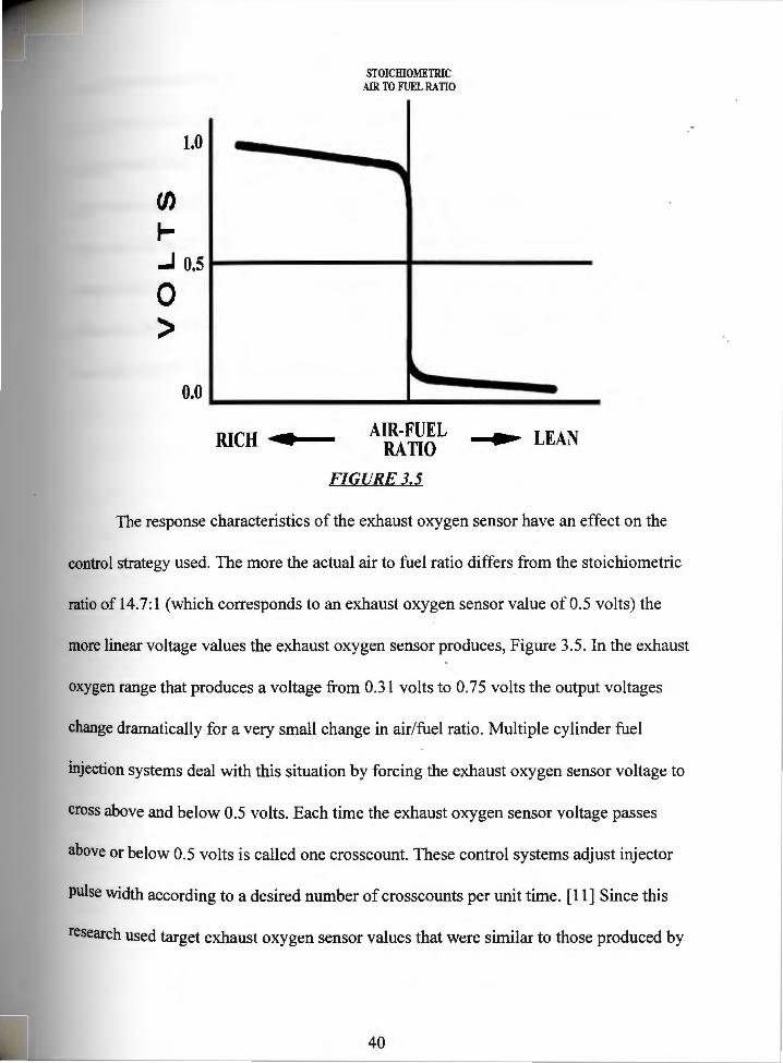
The response characteristics of the exhaust oxygen sensor have an effect on the

control strategy used. The more the actual air to fuel ratio differs from the stoichiometric

ratio of 14.7:1 (which corresponds to an exhaust oxygen sensor value of 0.5 volts) the

more linear voltage values the exhaust oxygen sensor produces, Figure 3.5. In the exhaust

oxygen range that produces a voltage from 0.31 volts to 0. 75 volts the output voltages

change dramatically for a very small change in air/fuel ratio. Multiple cylinder fuel

injection systems deal with this situation by forcing the exhaust oxygen sensor voltage to

cross above and below 0.5 volts. Each time the exhaust oxygen sensor voltage passes

above or below 0.5 volts is called one crosscount. These control systems adjust injector

pulse width according to a desired number of crosscounts per unit time. [11] Since this

research used target exhaust oxygen sensor values that were similar to those produced by

40

bureted engine, which were above 0.8 volts, a crosscount type control strategy was the car

eded In the voltage range above 0.75 volts the exhaust oxygen sensor values notne ·

change more linearly for a given change in air/fuel ratio. The integral action was the

most important portion of the control code. If the actual and target exhaust oxygen sensor

alue vary by an amount too small for the proportional gains to correct, the integral action v .

compensates. It modifies the base injector ontime in proportion to a summation of the

differences between target and actual exhaust oxygen sensor values over a period of time.

The exact proportion used is called the integral gain.

41

.CHAPTER 4 : COMPARISONS AND CONCLUSIONS

~ FLO-JET VERSUS PULSA-JET CARBURETOR

The first and perhaps most important aspect of any data acquisition device is the

repeatability. A test device must be able to repeat the same test and give close to the same

results before it can be considered a valid test. Figures 4.1 and 4.2 at the end of section

4.1 demonstrate the repeatability of the torque versus speed measurements for two

separate tests of the pulsa-jet carbureted engine. Once a data acquisition system has been

proven to give repeatable results, the next most important requirement is to produce

accurate results. If a sensor produces a one volt signal, the acquisition system is useless

unless it records something very close to a one volt signal. If the acquisition system

records a 3 volt signal, regardless of how many times it is repeated, it is of no scientific

use. To ensure the accuracy of the results, each of the data acquisition sensors, as well as

the analog to digital converter boards and computers were individually calibrated. It was

not possible to calibrate the dynamometer as a complete assembly with the reduction belt

drive in place.

An important comparison is one between the results achieved for the carbureted

engine as manufactured and the advertised torque and power curves achieved by the

factory for the same engine. This comparison demonstrates that the results from the

dynamometer are of the same order of magnitude as the expected test engine output

values. Once again, the results do not need to match exactly because all of the tests are

strictly comparisons performed on the same dynamometer. As one can see by comparing

42

figures 4.2 and 4.3, the torque and horsepower versus engine speed curves for the

tory test and the torque and speed curves provided by the factory are comparable. tabora

Table 4.1 highlights the important points on the torque graphs for Figures 4.1 A - 4.6A.

The key points on the Briggs & Stratton factory torque graph (Figure 4.3A) were 6.40

foot-pounds of torque at 1800 RPM, a peak torque of 7.65 foot pounds at 3000 rpm, and

7.30 foot pounds at 3600 rpm. The corresponding key points on the torque curve for the

pulsa-jet equipped test engine (Figure 4. lA) were 6.75 foot-pounds at 1800 RPM, a peak

torque of 7.1 foot pounds at 2700 RPM and 6.75 foot pounds at 3600 RPM. The two

torque curves have a similar shape, with the torque curve for the test engine peaking

earlier at 2700 RPM instead of at 3000 RPM. The test engine produced more low speed

torque, 5.5 % more at 1800 RPM, than the factory rating, but did produce 7.2 % less peak

torque and 7.5 % less torque at 3600 RPM. Table 4.2 highlights the important points on

the horsepower graphs for Figures 4.lB - 4.6B. The factory horsepower curve (Figure

4.3B) showed 2.2 horsepower at 1800 RPM, and a peak power of 5 .0 horsepower at 3600

RPM. The pulsa-jet equipped test engine produced 2.3. horsepower at 1800 RPM, an

increase of 4.5 %, but peaked at a 7 % lower 4.65 horsepower at 3600 RPM.

There are a number of factors that contribut_e to the lower torque and horsepower

production of the test engine compared to the factory specifications. The most evident is

the frictional losses in the dynamometer due to the reduction belt drive. Also a possible

contributing factor was the fact that the air filtration system was removed from the

carburetor of the test engine because the design and construction of a complete intake air

filtration system for the fuel injection system was not the intent of this research. The

43

ability between the factory specifications for the engine and the measured values coropar

for the engine demonstrates the validity of the test dynamometer apparatus.

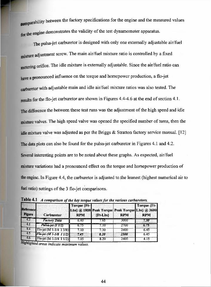
The pulsa-jet carburetor is designed with only one externally adjustable air/fuel

roixture adjustment screw. The main air/fuel mixture ratio is controlled by a fixed

roetering orifice. The idle mixture is externally adjustable. Since the air/fuel ratio can

have a pronounced influence on the torque and horsepower production, a flo-jet

carburetor with adjustable main and idle air/fuel mixture ratios was also tested. The

results for the flo-jet carburetor are shown in Figures 4.4-4.6 at the end of section 4.1.

The difference the between these test runs was the adjustment of the high speed and idle

mixture valves. The high speed valve was opened the specified number of turns, then the

idle mixture valve was adjusted as per the Briggs & Stratton factory service manual. [12]

The data plots can also be found for the pulsa-jet carburetor in Figures 4.1 and 4.2.

Several interesting points are to be noted about these graphs. As expected, air/fuel

mixture variations had a pronounced effect on the torque and horsepower production of

the engine. In Figure 4.4, the carburetor is adjusted to .the leanest (highest numerical air to

fuel ratio) settings of the 3 flo-jet comparisons.

Table 4.1 A comparison of the key torque values for the various carburetors.

'f(trqlle{).i't- 1forq11e{}?t­J_,~~}•••@\1801) Pelik •. Torqlle·~·J>eak'l'orque ·t~s} @~6()()

) }U>,M / ·•>•{Ft .. Lbs}··········~······ RPM.•)···•·•·• ••••••·•••••••••.RPM:·•• >•··

44

I 4 1 highlights the key points of the torque graphs for Figures 4.lA- 4.6A. The Tabe ·

. produced 7.10 foot-pounds of torque at 1800 RPM. It produced a peak torque of engme

30 foot pounds at 2400 RPM, and 6.45 foot pounds at 3600 RPM. The engine produced 7.

2.45 horsepower at 1800 RPM, and peaked at 4.40 horsepower at 3600 RPM. Figure 4.5

is the same flo-jet carburetor with the main jet opened to produce a richer mixture. These

settings produced 7.45 foot pounds of torque at 1800 RPM, peaked with 8.2 foot pounds

at 2500 RPM, and had 6.45 foot pounds at 3600 RPM.

Table 4.2 A comparison of the key horsepower values/or the various carburetors.

Horsepower@ Horsepower@ 1800 RPM 3600 RPM

4.3 Factory Data 2.20 5.00

4.l Pulsa-jet (1112) 2.30 4.65

4.4 Flo-jet (M 1-1/4 I 3/8) 2.45 4.40

4.5 Ro-jet (M 1-518 I 112) 2.50 4.40

4.6 Flo-jet (M l-3/4 I 112) 2.45 2.85

Highlighted areas indicate maximum values.

Table 4.2 compares the key points for the horsepower graphs in Figures 4. lB- 4.6B. The

engine produced 2.5 horsepower at 1800 RPM and 4.4 at 3600 RPM. Figure 4.6 has the

richest air to fuel mixture of all of the carburetor tests. These settings produced 7 .15 foot

pounds of torque at 1800 RPM, peaked with 8.20 foot pounds at 2400 RPM, but had only

4.15 foot pounds at 3600 RPM. The engine produced 2.45 horsepower at 1800 RPM and

2.85 horsepower at 3600 RPM. The key points on the torque curve for the pulsa-jet

equipped test engine (from Figure 4.lA) were 6.75 foot-pounds at 1800 RPM, a peak

torque of 7.10 foot pounds at 2700 RPM and 6.75 foot pounds at 3600 RPM.

45

The flo-jet torque graphs (Figures 4.4A - 4.6A) demonstrated an increased

concavity as the air to fuel ratio was made richer. A torque graph with concavity is one

where the peak torque of the curve is higher, but the low and high speed torque values are

lower. In racing and other high performance arenas, this is called having a 'peaky' torque

curve. Peaky torque curves are not as desirable as 'flat' torque curves for racing

applications. The reasoning behind this is simple. If an engine has a peaky torque curve,

the engine RPM must be kept close to the peak torque speed. If the engine speed is

increased or decreased away from this peak speed, the amount of torque produced drops

off significantly. In most racing applications, a transmission would have to be shifted to

keep the engine operating at the desired speed. If the peak torque range is narrow, more

transmission gears are needed to keep the engine speed in the optimum range. This adds

to the weight of the machine, which decreases performance. It also adds more moving

parts which decreases reliability. In addition, the driver of the vehicle must shift more

often, which increases the chances the driver will make an error shifting the transmission.

If a racing engine has a flatter torque curve, it widens the optimum operating range, and

counters the above listed negative effects. The optimum torque curve for racing,

especially circle track racing, would be a straight horizontal line. This would correspond

to a constant torque output at all engine speeds. The pulsa-jet carburetor most closely

resembled the optimum, having a flatter torque curve than any of the curves produced

with the flo-jet carburetor.

The graphs also demonstrate that the maximum horsepower output decreases as

the air/fuel mixture is made richer. As the air/fuel mixture is made richer, the engine

46

rfi ance at higher RPM suffers. The extreme case is when the engine is so rich that it pe orm

will barely reach full operating speed under no load. Since no load torque is produced at

that speed, the net horsepower is zero.

Figures 4.4C, 4.SC, and 4.6C show the lambda sensor readings for each of the

three flo-jet carburetor mixture valve settings. Figure 4.1 C shows the lambda sensor

readings for the pulsa-jet carburetor. The settings in Figure 4.4 show the range of values

to be between 0.94 volts and 0.97 volts. Figures 4.SC and 4.6C show the lambda sensor

voltages for the other flo-jet data runs. These lambda sensor ranges are 0.98 volts - 0.96

volts and 1.02 volts - 0.97 volts, respectively. By automobile engine manufacturer' s

standards, anything over 0.50 is a rich mixture; over 0.80 is a very rich mixture. Because

the test engine is an L-head design, not an overhead valve design like a typical

automobile engine, the combustion and flow processes are less efficient and the engine

needs a richer mixture to run properly. Figure 4.1 C shows the exhaust oxygen sensor data

from the pulsa-jet carburetor. The pulsa-jet carburetor had a much broader range of

lambda sensor values, going from 0.92 volts down to 0.88 volts at 2200 RPM. Below

2200 RPM, the air to fuel ratio increased dramatically with the oxygen sensor values

dropping to 0.10 volts. This was typical of all of the pulsa-jet carburetor data sets. As the

engine speed dropped below 2200 RPM, the engine leaned out.

47

Torque vs Speed Pulsa-jet carburewr Idle 112

8.0

-"' 7.5

~ 7.0 I .... ~ 6.5 -Q,j

g. 6.0 ... = 5.5 !-

5.0 0 0 = e ~ 0 0 e 0 = 0 0 e 0 0 0 f::i "T \.Q QC) 0 N "T ~ QCI ... N N N N N !"') !"') !"') !"')

Engine Speed {RPM}

Pulsa-;et carburetor

Horsepower vs Speed Idle 112

6

5 ... Q,I 4 ~ = c. 3 Q,I

"' ... = 2 ::

1

0 0 0 e 0 0 0 g e 0 0 0 e e 0 ~ 0 0 0 QC) 0 N "T \.Q 0 N "T \.Q - N N N N N !"') !"') !"') !"')

Engine Speed {RPM}

Oxygen vs. RPM Pulsa-;et carbure/Or Idle 112

1.00 0.98 0.96 0.94 0.92 0.90 0.88 0.86 0.84 0.82 0.80

0 = e 0 e e e e e g e 0 e ~ e e e e :::: QCI

~ N 'C QC) e N "T \.Q

N N N N !"') !"') !"') !"')

48

Pulsa-jet carburetor Torque vs Speed Idle jet 112

9

- 8 "' J:J ..;i .!. 7 ~ u 6 ::I ~ .. s Q

!-"'

4

= = = = = = = = = = = = = = = = = = = = QC Q M ..., \C QO Q M ..., \C - M M M M M tr) tr) tr) tr)

Engine Speed {RPM}

Power vs Speed Pulsa-jet carburetor

Idle jet 1 12

s 4 ..

u ~ 3 Q c. u ~ 2 Q

::c 1

0

= Q Q Q Q Q Q Q Q Q = Q Q Q Q Q Q Q Q Q QO = M ..., \C QO Q M ..., \C - M M M M M tr) tr) tr) tr)

Engine Speed {RPM}

49

Figure 4.3 A Torque vs Speed

Engine Speed {RPM}

Pulsa-jet carburetor Factory provided curves

~===============-- --- ------ '============i

Figure 4.3 B

= = QC .... = = = N

= = N N

Horsepower vs Speed

= = ~ N

= = QC N

Engine Speed {RPM}

50

= = = f"'l

Pulsa-jet carburetor Factory provided curves

Figure 4.4 A

0 e 0 e QC ~ ....

Figure 4.4 B

5

4

1

0

i--i--:--

l e 0 QC -

e e e N

Figure 4.4 C

Torque vs Speed

I I T

e e s: e ~ ;::; ~ N M N N N

Engine Speed {RPM}

Horsepower vs Speed

i.....----1

'

Engine Speed {RPM}

Oxygen vs. RPM

l I

;:::;

1 i I I

e e e t"l

e ~ t"l

Flo-jet carburator main 1-114 idle 318

-'

= g ~ \0 t"l t"l

Flo-jet carburator main 1-114 idle 318

1 I

l

Flo-;et carburator main 1-114 idle 318

I

'

1.00 -,----~--~-------.----,.,--.----,----,------,------,

0.98 -i----- -+--- -+----+- ---,i------r.._---.... -t----t--- -+----1 0 .. M -A !"'II _e_l.\"'IM

0•96 ~:~:=:o=:::e=~a_=me=::=~•=~1t:=e::e::•r::·i-::-.~=·~:::::~"'~:~:=~ "'·:·,,-~:·w~=:o::o:~=~~:-:0:1...i:I~::::•~ u··: -'i" ~ ~ -0.92 -r-----+-! ----+---2-+----t-----t-- - -+--- -t---- -t-------1 0.90 -+---+i---+----t--y-c'-...:_,--i --,-f---__c_t--·:,,--:·-+---+---+-----1 0.88 -r-----+---+------+->-~f----+---+-----+---+1----i 0.86 -t----+-----+----+-'---- t-----+--- -+-----+----+-----1 0.84 -r-----+-----+- --+----'---+------+---+----+--- - --+----j 0.82 -t---+-- --+--- -+--- - -t-----+-- - -+----+-...,..--+----1 0.80 -i---- -+----+----+-----t---:----+----+----+--'---+- - --1

51

I L

Figure 4.5 A Torque vs Speed

Engine Speed {RPM}

Figure 4.5 B Horsepower vs Speed

Flo-jet carburator main 1-5/8 idle 112

Flo-jet carburator main 1-5/8 idle l /2

4 J___J~_J~_j_-=-~~:±:::::j1:=::t:::t=:j" ~ I

Engine Speed {RPM}

I

I _J

Figure 4.5 B Oxygen vs. RPM Flo-jet carburator main 1-5/8 idle 1/2

1.00 ~---------------~------------

0.98 ~1 ""'&.a --•·~wn:11~0ii';~-iiihii:-:-::-ii-t---:-,,.--l!l~ .• =---'el~Qiit3!mleeomGl"7""'fJ- I"· iio:tim~~~r-iii11iii.Diiiii-0i\• ii.-.--me-w~-H~ltmiiti .. .----.eli\11-m>l· 0.96 -1-==-=e~~l4-~~~~=-==i~~~~~~--;;~~~~ 0.94 -t---+----!----+----+---_,,_-1-----1f-------l-.:.::__----+-----1 0.92 -t----+------l----+---l----+----+------1-------+-----1

0.90 0.88 --r----+------1-----+---l----+----+------1-------+-- ··__,·

0.86 -t-----l----+---+---t------+-----1----l---~-----+----< 0.84 --r----+------1----+---l----+--~-+------1-------+-----I 0.82 -t---+----+------l-----1----l-------1----1----1-------'

0.80 --r-----1-----+--- -+- --t------+-----l----l-------+,----I e e e N

e e N N

e e ~ N

52

e e ac N

e e e (")

e e ~ (")

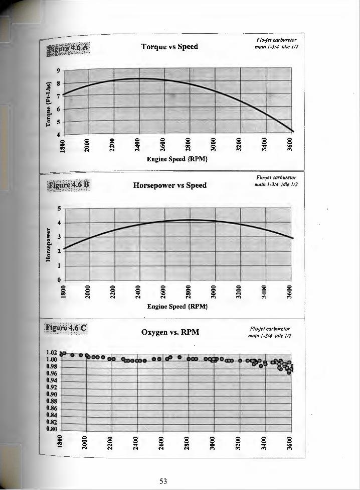
Flo-jet carburetor

Torque vs Speed main 1-314 idle 112

9

';ii' 8 ~

7 ~ e Qj 6 :I r:1' .. c:> s !-"'

4

= = = = = = = = = = = = = = = = = = = = 00 = N ""' l,C CIC = N ""' l,C

.... N N N N N !") !") !") !")

Engine Speed {RPM}

Flo-jet carburetor

Horsepower vs Speed main 1-314 idle 112

s

4 .. Qj

~ 3 c:> c. Qj

"' .. 2 c:>

:i:: 1

0

= = = = = = = = = = = = = = = = = = = = CIC = N ""' l,C CIC = N ""' l,C .... N N N N N !") !") !") !")

Engine Speed {RPM}

Oxygen vs. RPM Flo-jet carburetor main 1-314 idle 112

1.02 1.00 0.98 0.96 0.94 0.92 0.90 0.88 0.86 0.84 0.82 0.80

= = = = = = = = = = = QO = = = = = = = = = .... = N ""' l,C QO = N ""' l,C N N N N N !") !") !") !")

53

¢QNSTANT PULSE WIDTH FUEL INJECTION

The first electronic fuel injection system that was tested for this experiment

d a constant pulse width control strategy. In actuality, it was a basic open loop feature

control system. A specified amount of fuel was injected into the engine regardless of the

actual engine requirements. This sort of control system is not very practical on a vehicle

application because the air to fuel ratio requirements change dramatically for different

throttle positions and engine loads. The test engine started and idled smoothly with 1 to 2

millisecond injection pulse widths, but had poor throttle response and stalled out under

even minimal external load. Pulse widths in the range of 3 to 5 milliseconds had a

moderately rough idle but had excellent throttle response and smooth high speed no load

operation. The engine did produce good torque and horsepower in this pulse width range.

Pulse widths in the 6 and 7 millisecond range produced a poor, choppy idle, excellent

throttle response, and good low speed torque. The air to fuel mixture was too rich for no

load operation and the engine misfired at high speed with zero load.

All of the lambda sensor voltages for pulse widths greater than 3.5 milliseconds

followed the same general trend. The ·sensor voltage remained constant from 3600 RPM

down to approximately 3000 RPM. The sensor voltage increased as the engine speed

slowed from 3000 RPM down to 1800 RPM. The average increase was about 0.04 volts.

This means that as the engine speed decreased, the amount of fuel required per revolution

decreased slightly. Figure 4.11 C demonstrates this general trend. For the pulse widths

under 3.5 milliseconds (Figures 4.7 and 4.8) the sensor voltage curves were virtually

54

. the ultra-lean range of 0.05 to 0.10 volts. Figure 4.8C shows a small rise in constant m

sensor voltage at 2400 RPM.

I 4 3 A comparison of the key torque values for the ftXed pulse width fuel injection. Tab e ·

5.0 6.85 5.5 6.80 6.0 7.20 7.0 7.00

Highlighted areas indicate maximum values.

Table 4.4 A comparison of the key horsepower values for the ftxed pulse width fuel injection .

; ):Injection Reference Figure Pillsewidtb {ms}

4.07 2.5 4.08 3.0 4.09 3.5 4.10 4.0 4.11 5.0 4.12 5.5 4.13 6.0 4.14 7.0

. Horsepower@ .. Horsep(j~r@··· 1800 RPM 3600RPM ii

2.25 3.70 2.25 4.30 2.25 4.90 2.40' 4.85 2.35 5.00 2.35 5.20 2.45 4.95 2.40 4.85

Highlighted areas indicate maximum values.

Figures 4.7- 4.14 are the torque, horsepower and lambda sensor values for the

fixed pulse width fuel injection tests. Table 4.3 highlights all of the torque values at 1800

RPM, 3600 RPM and peak torque point. Table 4.4 highlights the horsepower values at

1800 RPM and at 3600 RPM. A fixed pulse width of 6 milliseconds produced the most

torque, 7 .2 foot pounds, at 1800 RPM. A leaner pulse width of 5 .5 seconds produced the

highest peak torque of 7.6 foot pounds at 3400 RPM, and also the most torque at 3600

RPM, 7.6 foot pounds. The best horsepower values were produced by the same two

55

. . ontimes. The 5.5 millisecond ontime produced 2.5 horsepower at 1800 RPM. inJectton .

The 6 millisecond ontime produced a maximum of 5.2 horsepower at 3600 RPM. One of

. portant things to note is that the horsepower curves did not peak at 3600 and begin the 1m

to decline, as the carburetor horsepower curves did. The peaky torque curves of the

carbureted engine tests dropped sharply after their maximum values. This sharp drop

forces the horsepower curves to peak out and begin to decline also. The flatter torque

curves of the fuel injected engine do not correspond to a peak to the horsepower curve

within the 1800 RPM to 3600 RPM operating range of the engine like the carbureted

engine did. For most racing applications, the engine is modified to raise the top operating

speed. Typical Briggs & Stratton go-cart racing engines are modified to run at speeds of

up to 8000 RPM. The increase in horsepower, especially at higher speeds, is perfectly

suited to racing applications. Raising the RPM at which the engine produces the

maximum torque and maximum horsepower is a marked improvement over a carbureted

engine. Therefore, even the basic open-loop fuel injection system is a substantial

improvement over a carburetor.

56

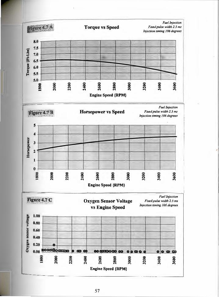
8.0

- 7.5 "' ~ 7.0 I ....

I "' - 6.5 II ::s ~ ... 6.0 Q

5.5 !-"'

5.0

= = 00 ...

r I I I I

! 5

4 ... II ~ 3 Q Q. II

"' ... 2 Q ::

1

0

= = 00

II 1.00 tlll ea ... Q 0.80 ;.. ...

0.60 Q

"' c II 0.40 "' c II tlll .... ~

0.20

0 0.00

= = QO -

= = = = = N N N

= = = N

= = = = = N N N

Torque vs Speed

= = = = = = ..., IQ 00 N N N

Engine Speed {RPM}

Horsepower vs Speed

Engine Speed {RPM}

Oxygen Sensor Voltage vs Engine Sp.eed

= = = = = = ..., IQ 00 N N N

Engine Speed {RPM}

57

Fuel Injection Fixed pulse width 2.5 ms

Injection timing I 06 degrees

Fuel Injection Fixed pulse width 2.5 ms

Injection timing 106 degrees

Fuel Injection Fixed pulse width 2. 5 ms

Injection timing 106 degrees

-~ ~ GI :s r:J' .. 0

!-""

L

.. GI ~ 0 Cl. GI

"' .. 0 :i::

GI QI)

" -c > ... Q

"' c: GI

171 c: GI QI)

~ 0

8.0

7.5

7.0

6.5

6.0

5.5

5.0

= = = = QCI = .... M

5

4

3

2

1

0

= = = = QCI 0 .... M

1.00

0.80

0.60

0.40

0.20

0.00 0 = QC) -

Torque vs Speed

Engine Speed {RPM}

Horsepower vs Speed

Engine Speed {RPM}

Oxygen Sensor Voltage vs Engine Speed

Engine Speed {RPM}

58

Fuel Injection Fixed pulse width 3 ms

Injection timing l 06 degrees

Fuel Injection Fixed pulse width 3 ms

Injection timing I 06 degrees

Fuel Injection Fixed pulse width 3 ms

Injection timing I 06 degrees

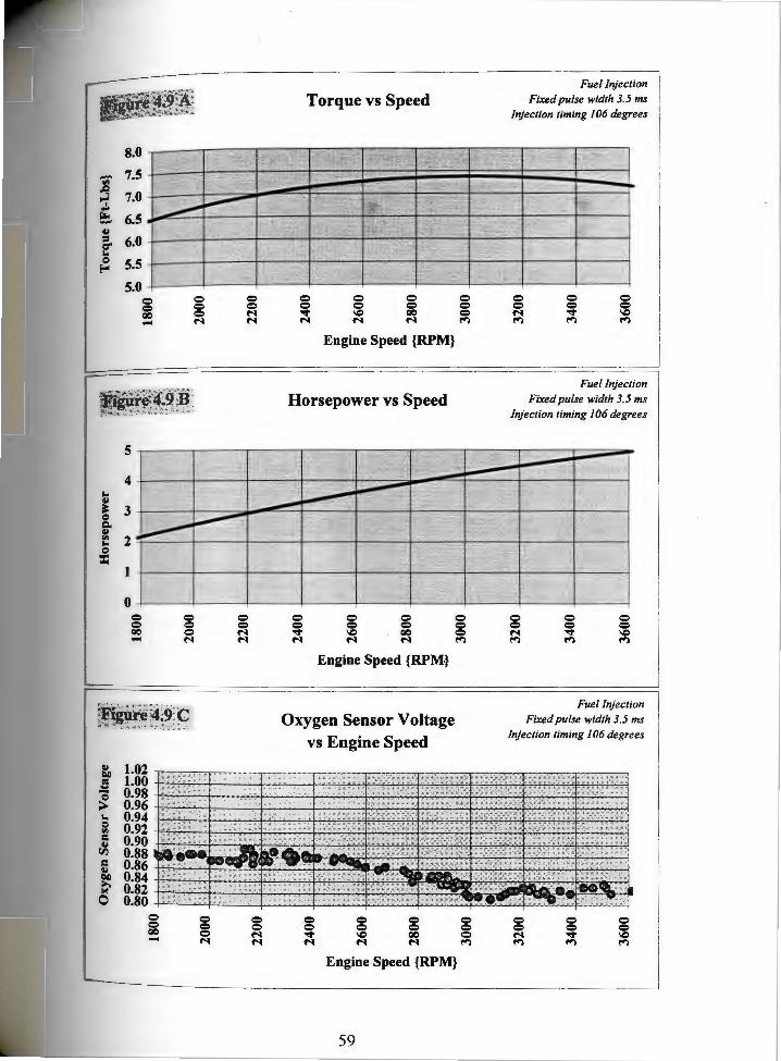
8.0

- 7.S "' ~ 7.0 ..!. ~ 6.S II = ~ ... 6.0 0 s.s !-"

s.o = = QC ...

s

4 ... GI ~ 3 0 c.. GI

"' ... 2 0 ::c

1

0

= = QC ...

GI 1.02 QI)

" 1.00 ... 0.98 0

> 0.96 ... 0.94 0 0.92 "' = 0.90 GI rr.i 0.88 = 0.86 GI QI) 0.84 ..... 0.82 ~

0 0.80

= = QC) ... L

= = = = = N N N

= = = = = N N N

Torque vs Speed

Engine Speed {RPM}

Horsepower vs Speed

Engine Speed {RPM}

Oxygen Sensor Voltage vs Engine Speed

Engine Speed {RPM}

59

Fuel Injection Fixed pulse width 3.5 ms

Injection timing I 06 degrees

Fuel Injection Fixed pulse width 3.5 ms

Injection timing I 06 degrees

Fuel Injection Fixed pulse width 3.5 ms

Injection timing I 06 degrees

Figure 4~10 C ': . , . ,; ··---, " ': . :~~c

~ 1.02 Oii 1.00 = 0.98 ... 0 0.96 > 0.94 ... 0 0.92 I

"' 0.90 c: ~ 0.88 'IJ c: 0.86 ~ 0.84 ~ 0.82 IJC

0.80 0 = = QO -

Oxygen Sensor Voltage vs Engine Speed

Engine Speed {RPM}

60

Fuel Injection Fixed pulse width 4 ms

Injection timing I 06 degrees

8.0

- 7.S "' ~

7.0 ...;i ~ ~ 6.S GI = 1:1' .. 6.0 e s.s !-"'

s.o = = = = 00 = .... N

s

4 .. GI

~ 3 e Clo GI

"' .. 2 e ::

1

0

= = = = 00 = - N

Figure 4.t)'c;

GI 1.02 1)11

1.00 ~ ... 0.98 Q

> 0.96 ... 0.94 e 0.92 .., = 0.90 GI

rJ') 0.88 = 0.86 GI 1)11 0.84 ....

0.82 ~

0 0.80

= = 00 -

= = N N

= = N N

Torque vs Speed

= = = = = = ...,. IC 00 N N N

Engine Speed {RPM}

Horsepower vs Speed

= = = = = = ...,. IC 00 N N N

Engine Speed {RPM}

Oxygen Sensor Voltage vs Engine Spee<J

Engine Speed {RPM}

61

Fuel ltyection Fixed pulse width 5 ms

Injection timing 106 degrees

Fuel Injection Fixed pulse width 5 ms

Injection timing 106 degrees

Fuel Injection Fixed pulse width 5 ms

Injection timing 106 degrees

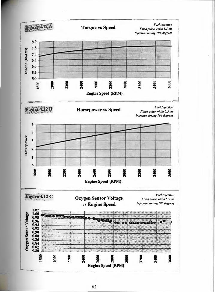
8.0

- 7.S "' ~ 7.0 I ...

[;Jo - 6.S GI ::s r:r 6.0 .. 0 s.s !--"

s.o = = = = QC = .... N

s

4 .. GI

~ 0 3 c. GI

"' .. 2 ~ ::c

1

0

= = = Q QC Q - N

Figure 4~12 C ' 'm-· =-

= = N N

= = N N

Torque vs Speed

Engine Speed {RPM}

Horsepower vs Speed

Engine Speed {RPM} .

Oxygen Sensor Voltage vs Engine Speed.

1.02 -,,.---.----.---.---:-i--:~-:;-:z

ti 1.00 ~~~~~!ii~ua .. ;;=;;;J~~~ !! 0.98 ::+ ~ 0.96 +.;.......:.:::....:.:::.J--_ _:......f-:-----t-~-'-"1'

0.94 F--:::-...,.-+~-+--+:-""T?T~ 0.92 *7--~'---f---'-0.90 0.88 -f"------:---''--t

= 0.86 +--~-+ ~ 0.84 +..:..~--+ 0 0.82 +---i--::2---::2-~~~~

0.80 ..j.L..:...__::.q....:.:::..:..._;.+--=..c~q.==~==-g 00

Q Q Q N

Q Q N N

g g g g ""' \C 00 Q N N N f"I

Engine Speed {RPM}

62

Fuel Injection Fixed pulse width 5.5 ms

Injection timing 106 degrees

Fuel Injection Fixed pulse width 5.5 ms

Injection timing 106 degrees

Fuel Injection Fixed pulse width 5.5 ms

Injection timing 106 degrees

8.0

- 7.5

~ 7.0 I .... ~ 6.5 Cll ::I 6.0 r3' .. 0 5.5 !-""

5.0

= = = = 00 = ... M

5

4 .. Cll ~ 3 0

"" Cll

t! 2 0

= 1

0

= = = = 00 = .... M

Figure4~13 C

Cll 1.02 t)I) 1.00 Ill ... 0.98

~ 0.96 .. 0.94 0 0.92 "' = 0.90 Cll

flJ 0.88 = 0.86 Cll

~ 0.84 ~ 0.82 0 0.80

= = 00 ....

= = M M

= = M M

Torque vs Speed

= = .., M

Engine Speed {RPM}

Horsepower vs Speed

= = = = = = .., IQ 00 M M M

Engine Speed {RPM}

Oxygen Sensor Voltage vs Engine Speed

Engine Speed {RPM}

63

Fuel Injection Fixed pulse width 6 ms

Injection timing I 06 degrees

Fuel Injection Fixed pulse width 6 ms

Injection timing 106 degrees

Fuel Injection Fixed pulse width 6 ms

Injection timing 106 degrees

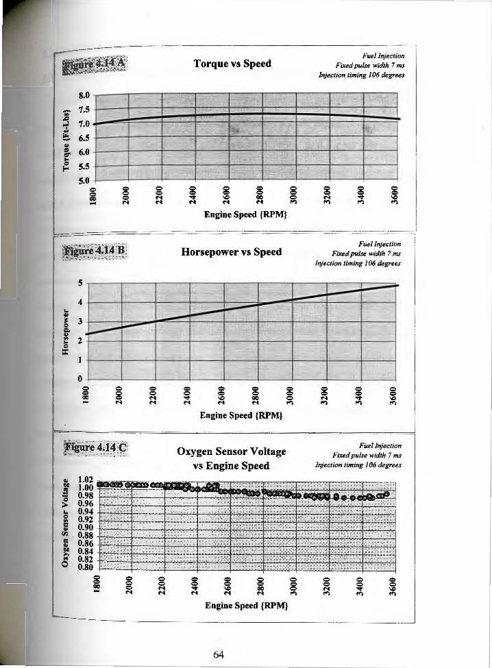
8.0

-"' 7.5 SJ

7.0 ..;i I ...

f:!, 6.5 II :::s er .. 6.0 c:> 5.5 !-"'

5.0 c::> c::> c::> = go = .... M

5

4 .. II ~ 3 Q c. II

"' .. 2 Q

::c 1

0 c::> = c::> = go = - M

~ 1.02 Cl! 1.00 = ... 0.98 ~ 0.96 .. 0.94 Q 0.92 "' = 0.90 ~ rlJ 0.88 = 0.86 ~ Cl! 0.84 '"' ~ 0.82 0 0.80

= = = = 00 = - M

= = M M

= = M M

Torque vs Speed

= = = = = = = = ..,. \C 00 = M M M ~

Engine Speed {RPM}

Horsepower vs Speed

= = = = = = ..,. \C 00 M M M

Engine Speed {RPM}

Oxygen Sensor Voltage vs Engine Speed

= = = ~

Engine Speed {RPM}

64

Fuel Injection Fixed pulse width 7 ms

Injection timing 106 degrees

Fuel Injection Fixed pulse width 7 ms

Injection timing 106 degrees

Fuel Injection Fixed pulse width 7 ms

Injection timing 106 degrees

~QSED LOOP FUEL INJECTION

!lJ.-fixed J 06° injection timing. varied oxy~en sensor target

As mentioned previously, open loop fuel injection is not particularly useful for

any real world application. Pulse widths which create the most torque and horsepower

result in poor idling and inferior performance under no load. At the pulse widths that the

engine idles smoothly, it has poor throttle response and terrible full-load power. Simply

stated, a gasoline engine needs a different air to fuel ratio for virtually every combination

of engine speed, throttle position, and external load. For a fuel delivery system to be

practical and useful, it has to change the amount of fuel delivered to the engine to

accommodate these different conditions. The lambda sensor provides an excellent method

to adjust the fuel delivery while the engine is in operation. The control system compares

the current oxygen sensor voltage with the desired voltage value, then adjusts the fuel

injector ontime to richen or lean the mixture as required. The fuel injection trigger was

initially set to 106° before the intake valve began to open. All of the variable pulse width

fuel injection data used the same proportional and integrnl gains. The proportional gain

was 10, the integral gain was 2, and both were used to modify a constant value of 5.0

milliseconds. The graphs of the first set of data are figures 4.15 - 4.19. All variables for

these data runs are identical with the exception of the target exhaust oxygen sensor value.

Injection timing was set to 106° before the intake valve began to open. Table 4.5

highlights the key points of the torque graphs.

65

Table 4. 5 A comparison of the key torque values for the variable pulse width fuel injection with

injection timing of I 06 ° and various oxygen target values.

,-- Oxygen Sensor Injection Torque{Ft- Peak Peak Torque {Ft-

Reference Target Timing Lbs} @l800 Torque {Ftl Torque Lbs} @3600

Figure Voltage degrees RPM Lbs} RPM RPM

~4. 15 0.85 106 6.70 7.20 3000 7.05

1-------4. 16 0.88 106 6.90 7.20 2700 6 .95

~.17 0.91 106 6.80 6.90 2600 6.70

i-- 4.18 0.92 106 .7.10 -c:;

7.25 2600 7.05

I- 4.19 0.95 106 6.95 7. 15 2700 6.95

Highlighted areas indicate maximum values.

Leaner air to fuel ratios generally produced more torque at higher engine speeds. A target

lambda sensor voltage of 0.85 volts and 0.92 volts produced the highest torque at 3600

RPM with 7.05 foot pounds. The target value of 0.92 volts also produced the most torque

at low speed with 7.1 foot pounds at 1800 RPM. The best peak torque was 7.25 foot

pounds at 2600 RPM produced by a target lambda sensor voltage of 0.92.

Table 4. 6 A comparison of the key horsepower values for the variable pulse width fuel injection

with injection timing of 106 ° and various oxygen target values.

Reference Horsepower @ Horsepower @ 1800RPM . 3600RPM

4.15 106 2.30 4.85 4.1 6 106 2.35 4.75 4.17 0.91 106 2.35 4.60 4.18 0.92 106 2.45 4.85 4.19 0.95 106 2.40 4.75

Highlighted areas indicate maximum values.

66

Table 4.6 highlights the key points of the horsepower curves. As expected the maximum

e Points at 1800 RPM and 3600 RPM produce the peak horsepower values at the torqu

same points. At 1800 RPM, the 0.92 oxygen sensor target voltage produced the best

power at 2.45 horsepower. The best top RPM horsepower was produced by two lambda

sensor targets, one of 0.85 volts, and the other of 0.92 volts. These settings each produced

4.85 horsepower at 3600 rpm.

67

8.0

-"' 7.S

~ 7.0 I

.:::: 6.S -Qj

= 6.0 1:1' .. e s.s E""

s.o = = = = ao = .... N

s

4 .. Qj

~ 3 e Q. Qj

~ 2 e = 1

0

= = = = ao = - N

Figure 4.l"S'c '=J:.

Qj 1.00 QI)

0.98 ea .... 0.96 ~ 0.94 .. 0.92 Q

"' 0.90 c Qj 0.88 [I}

c 0.86 Qj

0.84 QI) ..... 0.82 "" 0 0.80

= = = = QO = - N

= = N N

= = N N

Torque vs Speed

= = = = = = ..... \C ao N N N

Engine Speed {RPM}

Horsepower vs Speed

= = = = = = ..... \C ao N N N

Engine Speed {RPM}

Oxygen Sensor Voltage vs Engine Speed

Engine Speed {RPM}

68

= = = !")

Variable pulse width injection Oxygen sensor target 0.8Sv

Injection timing 106 degrees

= = N !")

Variable pulse width injection Oxygen sensor target 0.8Sv

Injection timing I 06 degrees

Variable pulse width injection Oxygen sensor target 0.8Sv

Injection timing I 06 degrees

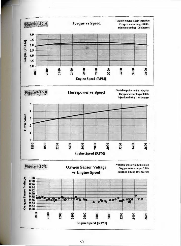
8.0

- 7.5 "' ~ 7.0

~ 6.5 41 = 6.0 ~ ... 0 5.5 !-"

5.0 = = = = = QC) N ....

5

4 ... 41 ~ 3 0 Q. 41

"' 2 ... 0 :c

1

0 = 0 = = 00 0 - N

Figure 4.i6c

~ 1.00 tlAI 0.98 Oil -= 0.96

> 0.94 ... 0.92 0

"' 0.90 = ~ 0.88, "1

= 0.86 ~ 0.84 tlAI ...... 0.82 ~

0 0.80 = = QC) ....

= = N N

= = N N

Torque vs Speed

g = = = = ..,. \C QC)

N N N

Engine Speed {RPM}

Horsepower vs Speed

= = = = = = ..,. \C QC) N N N

Engine Speed {RPM}

Oxygen Sensor Voltage vs Engine Speed

Engine Speed {RPM}

69

= = = !")

Variable pulse width injection Oxygen sensor target 0.88v

Injection timing I 06 degrees

= = N !")

Variable pulse width injection Oxygen sensor target 0.88v

Injection timing l 06 degrees

Variable pulse width injection Oxygen sensor target 0.88v

Injection timing l 06 degrees

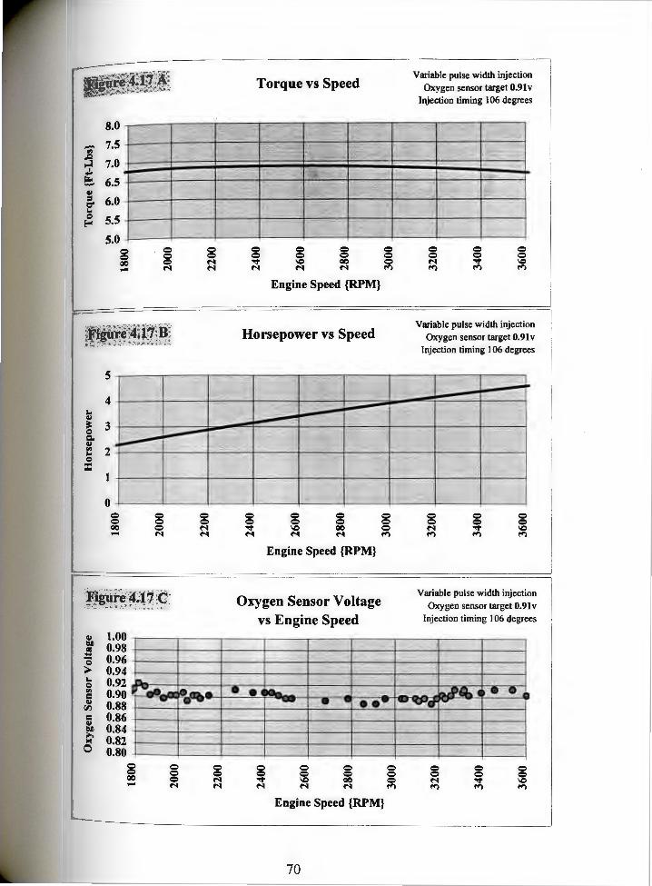
8.0

- 7.5 "' J:l

7.0 ..;i .:. r;i;. 6.5 -GI ::I 6.0 a" .. 0 5.5 !-"

5.0

= = = = CIO = ... M

5

4 .. GI ~ 3 0 c. GI

"' .. 2 0

::i::: 1

0

= = = = CIO = - M

Q,j 1.00 tlfl 0.98 OI - 0.96 Q > 0.94 .. 0.92 0

"' 0.90 = Q,j 0.88 fl)

= 0.86 Q,j

0.84 tlfl ..... 0.82 lo'l 0 0.80

= = CIO -

= = M M

= = M M

Torque vs Speed

= g = = = ..., IC CIO M M M

Engine Speed {RPM}

Horsepower vs Speed

g = = = = ..., IC CIO M M M

Engine Speed {RPM}

Oxygen Sensor Voltage vs Engine Speed

Engine Speed {RPM}

70

Variable pulse width injection Oxygen sensor target 0.9lv

Injection timing l 06 degrees

Variable pulse width injection Oxygen sensor target 0.91 v

Injection timing 106 degrees

Variable pulse width injection Oxygen sensor target 0.91 v

Injection timing 106 degrees

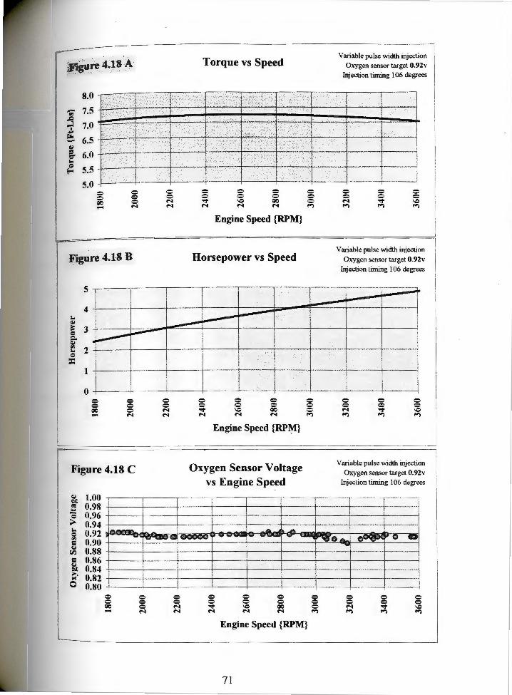
Figure 4.18 ~

8.0 - 7.5 "'

L.. ;~, > -;c

.t:l ~ 7.0 I .. ' I> " ,"

ti_ < ~ - 6.5 ~ = r:;' 6.0 ... Cl 5.5 Eo-

5.0

I'• --'-

v--

= = = N

Figure 4.18 B

1

Figure 4.18 C

I' .

0 = N N

.C-

Torque vs Speed

'"'

-=- 2 '

-0 .-?' s ~ '_:._'. :,,

----- ->i < . : "-"

"~ >

'

0 0 OCI N

_;_

'

_'

Engine Speed {RPM}

Horsepower vs Speed

Engine Speed {RPM}

Oxygen Sensor Voltage vs Engine Speed

0 0 = l"'l

"

Variable pulse width injection Oxygen sensor target 0.92v

Injection timing I 06 degrees

Variable pulse width injection

Oxygen sensor target 0.92v Injection timing I 06 degrees

Variable pulse width injection Oxygen sensor target 0.92v

Injection timing I 06 degrees

~ 1.00 ~~~~~~~~~~--.~~~,---~~-.-~~----,~~~--,--~~-,~~---,

~ 0.98 -+-~~-+~~~-t---~~-r~~~r-~~-t-~~---i~~~-+-~~--t~~--1

~ 8:~~ -+----+----+-- --+----r----t----t----+----+-----1

~ 0.92 "!~' 1"'fJ-'""'o-g- •· 'tl --1-t:-~~ljq-«-!i- e1c; a-tflR:5i:~~~--o~-ee- ~,, ... x.....,~-... H .... ~~~ ...... a- ~-t.P:Ji- ''-<lmQA~t;0;-, A.:i-;;0~;1-~------ ~pr.flr~'.'lua1:. ~ 8:~~ -+-~~-+-~~--+~~~+-~~-t-~~-+~~~+--~~-w~-~~~+-~~~ = 0.86 -+-~~-+-~~--+~~~+-~---t-~~-+~~~+--~~-+-~~-+~~--; ~ 0.84 +-~~-+~~~+-~~-t-~~~r-~~-t-~~~r--~~-t-~~--t~~--j

g 8::~ -+--- -+-- --+----r----t----+----+----+----+----;

= 0 OCI - 0 = N

0 = N N

= = "° N

0 = OCI N

Engine Speed {RPM}

71

8.0

,.,... "'

7.5 J:I ..J

I ... 7.0 ~ ...,., 6.5 Ill

= a' ... 6.0 0 5.5 Eo-

5.0

= = 0 = = 0 00 = N - N N

5

4 ... Ill ~ 3 0 Q. Ill

"' 2 ... 0

::r: 1

0

= = = = 0 = 00 0 N - N N

~ 1.00 I)!) ~ 0.98 ... 0 0.96 > 0.94 ... 0.92 0

"' 0.90 = ~ 0.88 [I)

= 0.86 ~ 0.84 I)!) >. 0.82 ~

0 0.80 = 0 0 0 00 0 - N

Torque vs Speed

= g 0 = 0 ...,. IC 00 N N N

Engine Speed {RPM}

Horsepower vs Speed

= = = = = 0 ...,. IC 00 N N N

Engine Speed {RPM}

Oxygen Sensor Voltage vs Engine Spee~

= = 0 f"I

= = = f"I

Engine Speed {RPM}

72

Variable pulse width injection Oxygen sensor target 0.95v

Injection timing I 06 degrees

0 0 0 0 0 = N ...,. IC f"I f"I f"I

Variable pulse width injection Oxygen sensor target 0.95v

Injection timing I 06 degrees

0 = 0 0 = 0 N ...,. IC f"I t'"I t'"I

Variable pulse width injection Oxygen sensor target 0.95v

Injection timing I 06 degrees

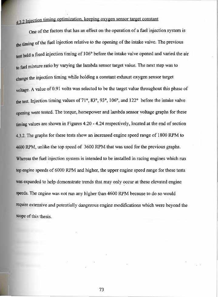
~njection timing optimization. keeping oxygen sensor target constant

One of the factors that has an effect on the operation of a fuel injection system is

the timing of the fuel injection relative to the opening of the intake valve. The previous

test held a fixed injection timing of I 06° before the intake valve opened and varied the air

to fuel mixture ratio by varying the lambda sensor target value. The next step was to

change the injection timing while holding a constant exhaust oxygen sensor target

voltage. A value of 0.91 volts was selected to be the target value throughout this phase of

the test. Injection timing values of 71°, 83 °, 93 °, 106°, and 122° before the intake valve

opening were tested. The torque, horsepower and lambda sensor voltage graphs for these

timing values are shown in Figures 4.20 - 4.24 respectively, located at the end of section

4.3.2. The graphs for these tests show an increased engine speed range of 1800 RPM to

4600 RPM, unlike the top speed of 3600 RPM that was used for the previous graphs.

Whereas the fuel injection system is intended to be installed in racing engines which run

top engine speeds of 6000 RPM and higher, the upper engine speed range for these tests

was expanded to help demonstrate trends that may only occur at these elevated engine

speeds. The engine was not run any higher than 4600 RPM because to do so would

require extensive and potentially dangerous engine modifications which were beyond the

scope of this thesis.

73

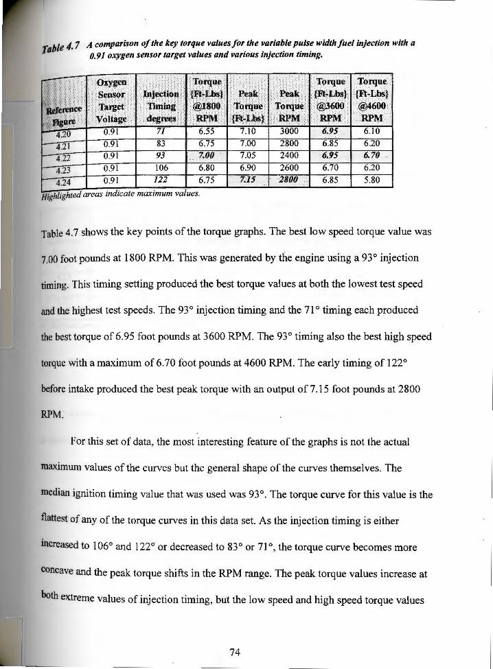
Table 4. 7 A comparison of the key torque values for the variable pulse width fuel injection with a 0.91 oxygen sensor target values and various injection timing.

4.21 0.91

4.22 0.91 7.00

4.23 0.91 106 6.80

4.24 0.91 122 6.75

Highlighted areas indicate maximum values.

7.05 2400

6.90 2600 7.15 2800

6.70

6.85

'' Torque>

:,{~:Lb$} '' ';@~90 ;; . Rl>M: >

6.10

6.20 6.70

6.20

5.80

Table 4.7 shows the key points of the torque graphs. The best low speed torque value was

7.00 foot pounds at 1800 RPM. This was generated by the engine using a 93° injection

timing. This timing setting produced the best torque values at both the lowest test speed

and the highest test speeds. The 93° injection timing and the 71° timing each produced

the best torque of 6.95 foot pounds at 3600 RPM. The 93° timing also the best high speed

torque with a maximum of 6. 70 foot pounds at 4600 RPM. The early timing of 122°

before intake produced the best peak torque with an output of 7 .15 foot pounds at 2800

RPM.

For this set of data, the most interesting feature of the graphs is not the actual

maximum values of the curves but the general shape of the curves themselves. The

median ignition timing value that was used was 93°. The torque curve for this value is the

flattest of any of the torque curves in this data set. As the injection timing is either

Increased to 106° and 122° or decreased to 83° or 71°, the torque curve becomes more

concave and the peak torque shifts in the RPM range. The peak torque values increase at

both extreme values of injection timing, but the low speed and high speed torque values

74

suffer losses. Once again, the high speed values are of the most significance, especially

bo 3600 RPM. The peaky torque curves show a significant decrease in torque at high a ve

ds which corresponds to a leveling off of the horsepower curve at the same speed. spee '

The horsepower curve for 93° injection timing was still rapidly increasing at 4600 RPM

while all of the other timing values had begun to level off.

Table 4.8 A comparison of the key horsepower values/or the variable pulse width fuel injection with a O. 91 oxygen sensor target value and various injection timing settings.

Figure 4.20 5.35

4.21 0.91 83 2.30 5.45

4.22 0.91 93 2.40 4.75 5.85

4.23 0.91 106 2.35 4.60 5.45

4.24 0.91 122 2.30 4.70 5.10

Highlighted areas indicate maximum values.

Table 4.8 shows the key points of the horsepower graphs. The 93° injection

timing was the best across the board for maximum horsepower production. Maximums

were 2.40 horsepower at 1800 RPM, 4.75 horsepower at 3600 RPM and 5.85 horsepower

at 4600 RPM. The 71° timing matched the 4.75 horsepower at 3600 RPM, but made 6.3

% less at 1800 RPM and 8.5 % less at 4600 RPM. The optimum value for injection

timing for this part of the experiment was 93 ° before the intake valve opens. If the vehicle

or machine that the injection system was being designed for were different, the optimum

injection timing for that application would likely have been different. For example, a

Pump with an operating speed of 2400 RPM to 3200 RPM might have been better suited

to use an injection timing of 122° because it had more torque in that RPM range. Since

75

the pumP would not need to operate out of this speed range, lower torque production at

other engine speeds is not detrimental. The flat torque curve and good high RPM torque

output of the 93° injection timing made it the optimum selection for a racing application.

76

8.0

-,,, ~

7.S

.,!. f;I;. - 7.0 GI = a'

6.S .. Q

!-"'

6.0

= = = = = 0 0 0 CIC 0 M ...,. .... M M M

6

s .. 4 GI ~ Q Cl. 3 GI ,,, .. Q 2 ::c

1

0

= 0 0 0 0 0 0 0 CIC 0 M ...,. - M M M

Figure'"4.2o c ~:/;,,.,, ;:>c:,-- .· ' ~;;;.:,,,

GI 1.00 t)I)

0.98 ~ .. 0.96 0

> 0.94 ... 0.92 Q

"' 0.90 = Cl.I 0.88 (l':J

= 0.86 Cl.I 0.84 t)I) ;.... 0.82 lo<! 0 0.80

0 0 0 0 0 0 0 0 CIC 0 M ...,. - M M M

Torque vs Speed

= = = 0 0 0 0 0 0 0 0 0 \C CIC 0 M ...,. \C M M I"') I"') I"') I"')

Engine Speed {RPM}

Horsepower vs Speed

0 0 \C M

0 0 0 0 0 0 0 0 0 0 CIC 0 M ...,. \C M I"') I"') I"') I"')

Engine Speed {RPM}"

Oxygen Sensor Voltage vs Engine Speed

0 0 0 0 0 0 0 0 0 0 0 0 \C CIC 0 M ...,. \C M M I"') I"') I"') I"')

Engine Speed {RPM}

77

0 0 CIC I"')

0 0 CIC I"')

0 0 CIC I"')

Variable pulse width injection Oxygen sensor target 0.91 v Injection timing 71 degrees

0 0 0 0 0 0 0 0 0 M ...,. \C ...,. ...,. ...,. ...,.

Variable pulse width injection Oxygen sensor target 0.91 v Injection timing 71 degrees

0 0 0 0 0 0 0 0 0 M ...,. \C ...,. ...,. ...,. ...,.

Variable pulse width injection Oxygen sensor target 0.91 v

injection timing 71 degrees

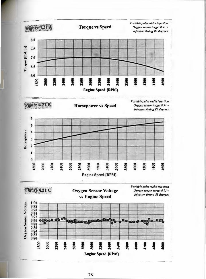
8.0

-"' 7.5 J:l ..;I ..:. ~ 7.0 GI :s ~

6.5 ... 0

E""'

6.0

= = = = = = = = 00 = M ...,. - M M M

6

5 ...

4 GI ~ 0 Q,. 3 GI

"' ... 0 2

= 1

0

= = = = = = = = 00 = M ...,. - M M M

Figtlre'.4~2f c , ···; -----;/ ,,,;, ->»>;'·.

GI 1.00 tiil Ill 0.98 -0 0.96 > 0.94 I. 0.92 Q

"' 0.90 = GI 0.88 f'1

= 0.86 GI 0.84 tiil ..... 0.82 l>Oi

0 0.80

= = = = = = QC = M M M

Torque vs Speed

= = = = g = = = = = = IQ 00 = M ...,. IQ M M f'"l f'"l f'"l f'"l

Engine Speed {RPM}

Horsepower vs Speed

= = = = = = = = = = = = IQ QC = M ...,. IQ M M f'"l f'"l f'"l f'"l

Engine Speed {RPM}·

Oxygen Sensor Voltage vs Engine Speed

Engine Speed {RPM}

78

= = 00 f'"l

= = QC f'"l

Variable pulse width injection Oxygen sensor target 0. 91 v Injection timing 83 degrees

= = = = = = = = = M ...,. IQ ...,. ...,. ...,. ...,.

Variable pulse width injection Oxygen sensor target 0.91 v Injection timing 83 degrees

= = = = = = = = = M ...,. IQ ...,. ...,. ...,. ...,.

Variable pulse width injection Oxygen sensor target 0.91 v

Injection timing 83 degrees

·1

!

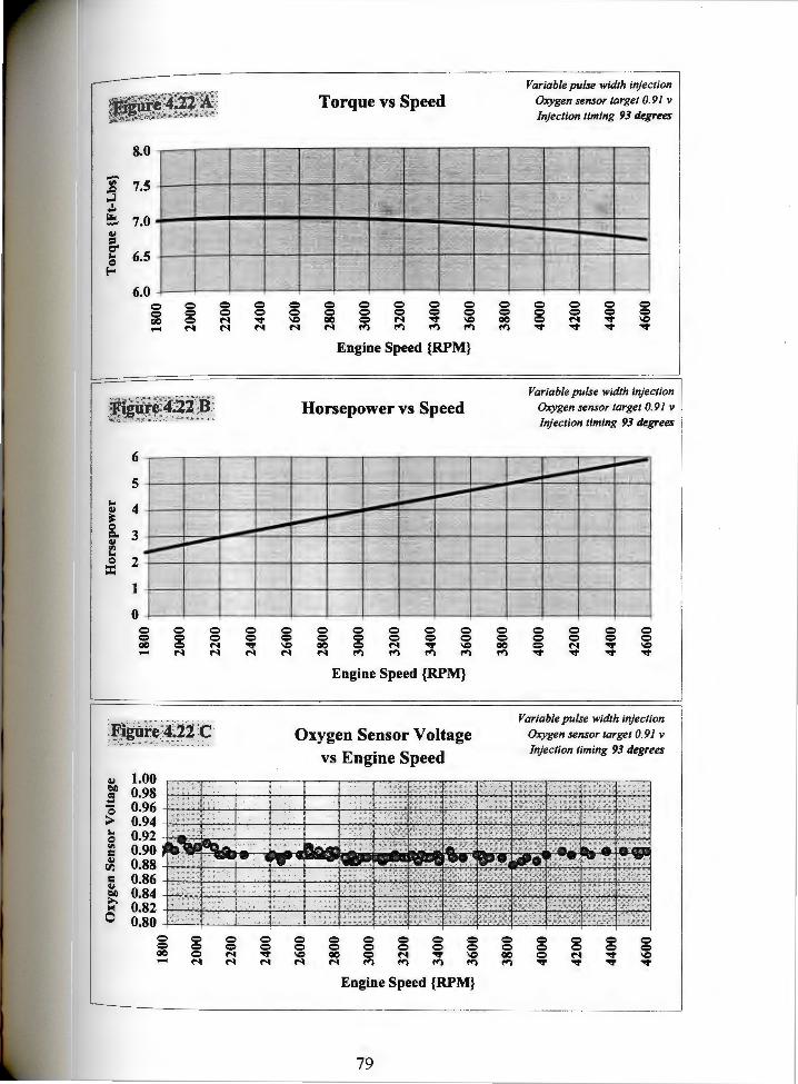
8.0

-"' ~ ..;i

7.5 .,.!. ~ 7.0 41 = i:3'

6.5 .. Q

E--

6.0 = = = = = = = = 00 = N ..., .... N N N

6

5 .. 4 41

~ Q c. 3 41

"' .. Q 2

::i:: 1

0

= = = = = = = = 00 = N ..., - N N N

Figii~e,4:22l-:! ;'.;J;: .. '

41 1.00 t:l.11 0.98 ~ - 0.96 Q > 0.94 .. 0.92 Q

"' 0.90 = 41 0.88 fl)

= 0.86 41

0.84 t:l.11 >. 0.82 ~

0 0.80

= = = = = = = = 00 = N ..., - N N N

Torque vs Speed

= = = = = = = = = = = = \C 00 = N ..., \C N N f"l f"l f"l f"l

Engine Speed {RPM}

Horsepower vs Speed

= = \C N

= = = = = = = = = = 00 = N ..., l,C N f"l f"l f"l f"l

Engine Speed {RPM}

Oxygen Sensor Voltage vs Engine Speed

= = = = = = = = = = = = l,C 00 = N ..., l,C N N f"l f"l f"l f"l

Engine Speed {RPM}

79

= = 00 f"l

= = 00 f"l

Variable pulse width injection Oxygen sensor target 0.91 v Injection timing 93 degrees

= = = = = = = = = N ..., \C ..., ..., ..., ...,

Variable pulse width injection Oxygen sensor target 0.91 v Injection timing 93 degrees

= = = = = = = = = N ..., \C ..., ..., ..., ...,

Variable pulse width injection Oxygen sensor target 0.91 v

Injection timing 93 degrees

8.0

-"' 7.5 .t:J ...;i

I .... ~ 7.0 GI ::s ~

6.5 "" 0

""" 6.0 0 0 0 0 0 0 ao 0 N .... N N

6

5

"" 4 GI ~ 0 c. 3 GI

"' "" 0 2 ::c: 1

0 0 0 0 0 0 0 0 0 ao 0 N ..,. - N N N

GI 1.00 Cl) 0.98 I'S ...

0.96 0 > 0.94

"" 0.92 0

"' 0.90 = GI 0.88 l;IJ

= 0.86 GI

0.84 Cl) >.

0.82 ~

0 0.80 0 0 0 0 0 0 ao 0 N - N N

0 0

'° N

0 0 ..,. N

Torque vs Speed

Engine Speed {RPM}

Horsepower vs Speed

0 0 0 0 0 0 0 0 0 0 ao 0 N ..,.

'° N ~ ~ ~ ~

Engine Speed {RPM} .

Oxygen Sensor Voltage vs Engine Speed

0 0 0 0 0 0 0 0 0 0 0 0

'° ao 0 N ..,. '° N N ~ ~ ~ ~

Engine Speed {RPM}

80

0 0 ao ~

0 0 ao ~

Variable pulse width injection Oxygen sensor target 0.9lv

Injection timing 106 degrees

Variable pulse width injection Oxygen sensor target 0.9lv

Injection timing 106 degrees

0 0 0 ..,.

Variable pulse width injection Oxygen sensor target 0.9/v

Injection timing 106 degrees

0 0 0 ..,.

8.0

-"' ,/:l ..;i ..!.

7.5

r::. 7.0 u ::I a'

6.5 "" 0 E-"

6.0 = = = = = = = = QQ = M ...,. ..... M M M

6

5

"" 4 u :r: 0 Q. 3 u "' "" 0 2 :c

1

0

= = = = = = = = QQ 0 N ...,. - M N M

Figure4:24 A

u 1.00 ~ 0.98 = - 0.96 Q > 0.94 "" 0.92 0

"' 0.90 = u 0.88 'J':J

= 0.86 u 0.84 ~ ..... 0.82

I

~

0 0.80 0 0 0 0 0 = 0 0

l QQ 0 M ...,. - M M M

Torque vs Speed

g = = = = = = = = = = IC QQ = M ...,. IC M M ~ ~ ~ ~

Engine Speed {RPM}

Horsepower vs Speed

= = IC M

= = = = = = = = = = QQ = M ...,. IC N ~ ~ ~ ~

Engine Speed {RPM}

Oxygen Sensor Voltage vs Engine Speed

0 0 0 0 0 0 0 0 0 0 0 0 IC QQ = M ...,. IC M M ~ ~ ~ ~

Engine Speed {RPM}

81

= = QQ ~

= = QQ ~

0 0 QQ ~

Variable pulse width injection Oxygen sensor target 0.9lv

Injection timing 122 degrees

= = = = = = = = = M ...,. IC ...,. ...,. ...,. ...,.

Variable pulse width injection Oxygen sensor target 0.9/v

Injection timing 122 degrees

= = = = = 0 0 0 0 M ...,. IC ...,. ...,. ...,. ...,.

Variable pulse width injection Oxygen sensor target 0.9/v

injection timing 122 degrees

0 0 0 0 0 0 0 M ...,. ...,. ...,. ...,.

U3 fixed 93° injection timing. varied oxygen sensor target values

Once the best injection timing value for the application was determined, the

engine output then was tested with the 93 ° injection timing and a variety of exhaust

oxygen sensor target voltage values. Figures 4.25 - 4.29 are the torque, horsepower, and

lambda sensor voltage graphs for the target oxygen sensor values of 0.85, 0.88, 0.91,

0.92, and 0.98 volts, respectively. Tables 4.9 and 4.10 show the key points of the torque

curves and horsepower curves, respectively.

Table 4. 9 A comparison of the key torque values for the variable pulse width fuel injection with a 93° injection timing and various oxygen sensor target values.

Reference Figure 4.25 4.26 0.88 7.10 6.95 6.05

4.27 0.91 93 7.00 6.95 6.70

4.28 0.92 93 7.25 7.30 2500 7.10 6.55

4.29 0.98 93 6.80 7.35 2800 7.00 5.60

Highlighted areas indicate maximum values.

Table 4.10 A comparison of the key horsepower values for the variable pulse width fuel injection with a 93° injection timing and v~rious oxygen sensor target values.

Reference Figure

Oxygen Sensor Injection HorsepolWr@ Horsepo~r@ B()~pOlWr@ Target Voltage Timing degrees 1800 RPM 3600RPM 4600RPM

4.25 0.85 93 2.40 4.85 5.45 4.26 0.88 93 2.45 4.75 5.30 4.27 0.91 93 2.40 4.75 5.85 4.28 0.92 93 2.50 4.85 5.75 4.29 0.98 93 2.35 4.80 4.90

Highlighted areas indicate maximum values.

Once again, the results showed trends very similar to the results in section 4.3.1 (106°

injection timing, various oxygen target values.) The target voltage on both the rich and

82

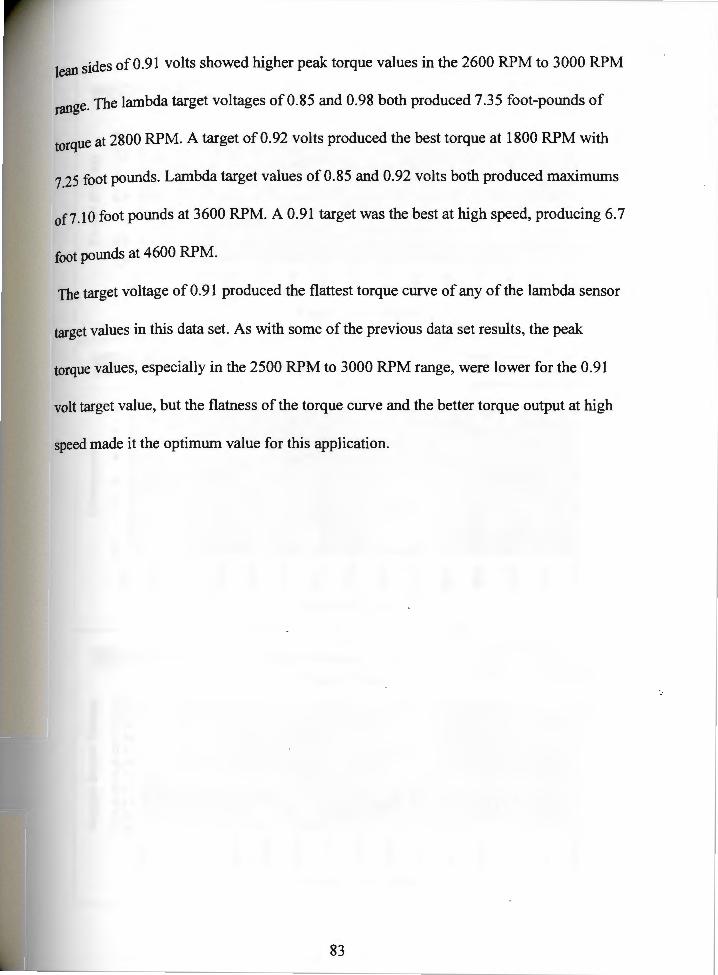
lean sides of 0.91 volts showed higher peak torque values in the 2600 RPM to 3000 RPM

range. The lambda target voltages of 0.85 and 0.98 both produced 7.35 foot-pounds of

torque at 2800 RPM. A target of 0.92 volts produced the best torque at 1800 RPM with

7.25 foot pounds. Lambda target values of 0.85 and 0.92 volts both produced maximums

of7.10 foot pounds at 3600 RPM. A 0.91 target was the best at high speed, producing 6.7

foot pounds at 4600 RPM.

The target voltage of 0.91 produced the flattest torque curve of any of the lambda sensor

target values in this data set. As with some of the previous data set results, the peak

torque values, especially in the 2500 RPM to 3000 RPM range, were lower for the 0.91

volt target value, but the flatness of the torque curve and the better torque output at high

speed made it the optimum value for this application.

83

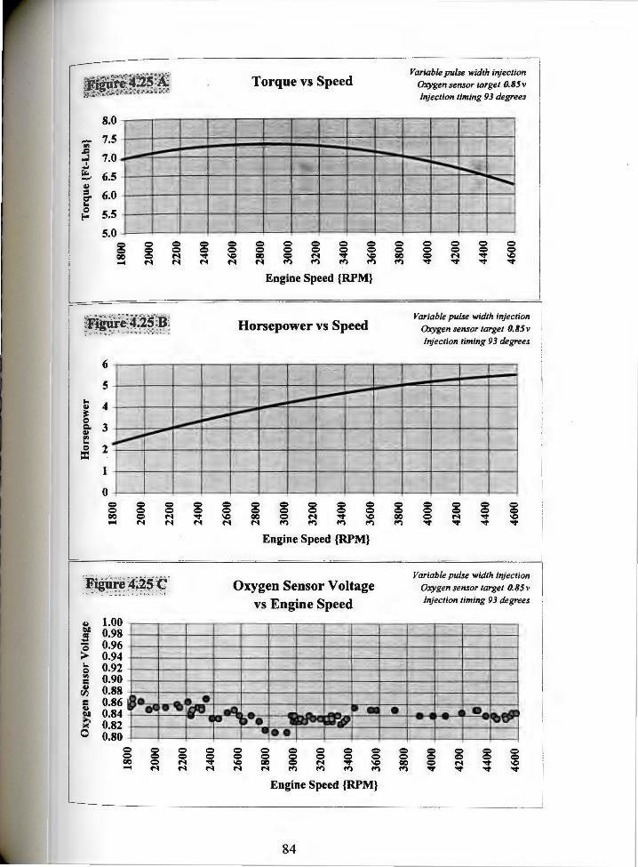
8.0

- 7.5 "' J:l

7.0 ..J .!. ~ 6.5 QI = 6.0 a' ... Q 5.5 ""' 5.0

0 0 0 0 0 0 0 0 QC 0 N ...,. .... N N N

6

5 ...

4 QI

~ Q c. 3 QI

"' ... Q 2 =

1

0 0 0 0 0 0 0 0 0 QC 0 N ...,. .... N N N

QI 1.00 1:)1) 0.98 = - 0.96 0 > 0.94 ... 0.92 Q

"' 0.90 = QI 0.88 VJ

= 0.86 41

0.84 1:)1) >. 0.82 ~

0 0.80 0 0 0 0 0 0 0 0 QC 0 N ...,. .... N N N

Torque vs Speed

0 0 0 0 0 0 0 0 0 0 0 0 IC QC 0 N ...,. IC N N !") !") !") !")

Engine Speed {RPM}

Horsepower vs Speed

0 0 IC N

0 0 0 0 0 0 0 0 0 0 QC 0 N ...,. IC N !") !") !") !")

Engine Speed {RPM}

Oxygen Sensor Voltage vs Engine Speed

0 0 0 0 0 0 0 0 0 0 0 0 IC QC 0 N ...,. IC N N !") !") !") !")

Engine Speed {RPM}

84

0 0 QC !")

0 0 QC !")

0 0 QC !")

Variable pulse width injection Oxygen sensor target 0.85v Injection timing 93 degrees

0 0 0 0 0 0 0 0 0 N ...,. IC ...,. ...,. ...,. ...,.

Variable pulse width injection Oxygen sensor target 0.85v Injection timing 93 degrees

0 0 0 0 0 0 0 0 0 N ...,. IC ...,. ...,. ...,. ...,.

Variable pulse width injection Oxygen sensor target 0.85v Injection timing 93 degrees

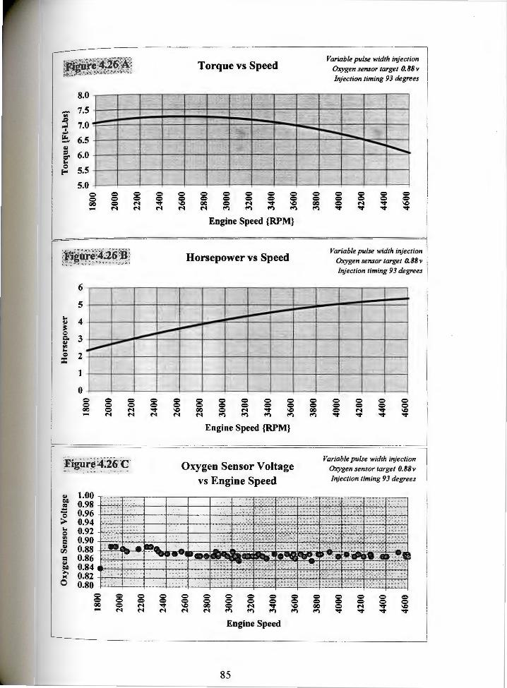
8.0

- 7.5 "' J:J, ~ .,!.

7.0

e 6.5 GI = r:r ... 6.0 0 5.5 E-<

5.0 c:> c:> c:> c:> c:> c:> c:> c:> go c:> M ..,. .... M M M

6

5 ...

4 GI

~ 0 c. 3 GI

"' ... 0 2 =

1

0 c:> c:> c:> c:> c:> c:> c:> c:> QC c:> M ..,. - M M M

GI 1.00 t)f)

0.98 t'I - 0.96 0 > 0.94 ... 0.92 0

"' 0.90 c GI 0.88 V1 c 0.86 GI

0.84 t)f) >. 0.82 lo< 0 0.80

c:> c:> c:> c:> = = = = QC = M ..,. - M M M

Torque vs Speed

c:> c:> g c:> c:> c:> c:> c:> c:> c:> c:> IQ go c:> M ..,. IQ M M ~ ~ ~ ~

Engine Speed {RPM}

Horsepower vs Speed

c:> c:> '° M

c:> c:> c:> c:> c:> c:> c:> c:> c:> c:> QC c:> M ..,. '° M ~ ~ ~ ~

Engine Speed {RPM}

Oxygen Sensor Voltage vs Engine Speed

c:> c:> c:> c:> c:> c:> = = = = = = '° QC = M ..,. '° M M ~ ~ ~ ~

Engine Speed

85

c:> c:> CIC ~

c:> c:> CIC ~

c:> = CIC ~

Variable pulse width injection Oxygen sensor target 0.88v Injection timing 93 degrees

c:> c:> c:> c:> c:> c:> c:> c:> c:> M ..,. IQ ..,. ..,. ..,. ..,.

Variable pulse width injection Oxygen sensor target 0.88v Injection timing 93 degrees

c:> c:> c:> c:> c:> c:> c:> c:> c:> M ..,. '° ..,. ..,. ..,. ..,.

Variable pulse width injection Oxygen sensor target 0.88v Injection timing 93 degrees

c:> = = ..,.

Figure 4.27 A

-"' ,::. ,.;i

I .... r-. _,., ~ = a' -0 ~

8.0

7.5

7.0

6.5

6.0

5.5

5.0 0 0 QC ....

_.-

0 0 0 N

Figure 4.27 B

6

5 -~ 4 :=: 0

fr 3 ~ i---" "' -0 2 =

1

0 ' 0

~ e e .... M

' 0 0 M N

l T r::i M

Figure 4.27 C

l

e e ~ = r::i M N

I '

-:;:;:: M

'

= :;:;:: M

Torque vs Speed

·•· : ;• ;

j i :j;< <

/ . I• : :~

Engine Speed {RPM}

Horsepower vs Speed

e 0 0 0

~ QC) = ~ e 0 ;;; ""' -:i

M M t') t') t')

Engine Speed {RPM}

Oxygen Sensor Voltage vs Engine Speed

!

I

' e e e 0 e

~ ~ = ~ e e ;;; ""' -:i

N M t') t') t')

Engine Speed {RPM}

86

0 e QC t')

e e QC t')

Variable pulse width in;ection Oxygen sensor target 0.91 v

Injection timing 93 degrees

c

Variable pulse width injection Oxygen sensor target 0.91 v

In;ection timing 93 degrees

0 e 0 0 0 0 e e e M ""' -:i

""' ""' ""' ""'

Variable pulse width injection Oxygen sensor target 0.91 v

ln1ection timing 93 degrees

e 0 e 0 0 e e e e M ""' -:i

""' ""' ""' ""'

8.0

-"' 7.5 ~

7.0 ..;i I ...

[:!, 6.5 ~ ::I 6.0 c:r "" 0 5.5 E-"'

5.0

I c::> c::> c::> c::> c::> c::> c::> c::> 00 c::> M ..,,. .... M M M

I I L

6

5

"" 4 ~

~ 0 c. 3 ~

"' "" 0 2 :c 1

0 c::> c::> c::> c::> c::> c::> = = 00 = M ..,,. - M M M

~ 1.00 ~ 0.98 C'I ....

0.96 0 > 0.94 "" 0.92 0 "' 0.90 = ~ 0.88 [I)

= 0.86 ~ 0.84 ~ >. 0.82 ~

0 0.80

= = = = = = = = 00 = M ..,,. .... M M M

Torque vs Speed

c::> c::> c::> c::> c::> c::> c::> c::> c::> c::> c::> c::> \C 00 c::> M ..,,. \C M M ~ ~ ~ ~

Engine Speed {RPM}

Horsepower vs Speed

c::> = \C M

c::> c::> c::> c::> c::> = = = = = 00 = M ..,,. \C M ~ ~ ~ ~

Engine Speed {RPM}

Oxygen Sensor Voltage vs Engine Speed

= = = = = = = = = = = = \C 00 = M ..,,. \C M M ~ ~ ~ ~

Engine Speed {RPM}

87

c::> c::> 00 ~

c::> = 00 ~

= = 00 ~

Variable pulse width injection Oxygen sensor target 0.92 v Injection timing 93 degrees

c::> c::> c::> c::> c::> c::> c::> c::> c::> M ..,,. \C ..,,. ..,,. ..,,. ..,,.

Variable pulse width injection Oxygen sensor target 0.92 v Injection timing 93 degrees

c::> c::> c::> c::> = = = = = M ..,,. \C ..,,. ..,,. ..,,. ..,,.

Variable pulse width injection Oxygen sensor target 0.92 v

Injection timing 93 degrees

8.0

-rll 7.5 ,&l

7.0 ..;i I ... ~ 6.5 -~ = 6.0 a'

"' 0 5.5 E--

5.0 = = = = = = = = 00 = N ..,, .... N N N

6

5

"' 4 ~

~ 0 c. 3 ~ rll

"' 0 2 ::i::

1

0 = = = = = = = = 00 = N ..,, - N N N

~ 1.00 bll 0.98 = - 0.96 Q > 0.94 "' 0.92 0 rll 0.90 = ~ 0.88 r.r.i

= 0.86 ~

0.84 bll ..... 0.82 ~

0 0.80 = = = = 0 = = = 00 = N ..,,

I I L

- N N N

Torque vs Speed

= = = = = = = = g = = = IQ QO N ..,, IQ N N f"I f"I f"I f"I

Engine Speed {RPM}

Horsepower vs Speed

= = IQ N

= = = = = = = = = = 00 = N ..,, IQ N f"I f"I f"I f"I

Engine Speed {RPM}

Oxygen Sensor Voltage vs Engine Speed

= = = = = = = = = = = = IQ 00 = N ..,, IQ N N f"I ~ ~ ~

Engine Speed {RPM}

88

= = 00 f"I

= = 00 f"I

= = 00 ~

Variable pulse width injection Oxygen sensor target 0.98 v Injection timing 93 degrees

= = = = = = = = = N ..,, IQ ..,, ..,, ..,, ..,,

Variable pulse width injection Oxygen sensor target 0.98 v Injection timing 93 degrees

= = = = = = = = = N ..,, IQ ..,, ..,, ..,, ..,,

Variable pulse width injection Oxygen sensor target 0.98 v

Injection timing 93 degrees

~ARBURETOR VERSUS FUEL INJECTION

The pulsa-jet carburetor, with its flatter torque curve and better high speed torque

production, as well as more dependable operation, proved to be the better of the two

carburetor systems tested. The final comparison was to see how well the pulsa-jet

carburetor would fair in a head-to-head competition with the electronic fuel injection

system. Figure 4.30 shows the best data from the pulsa-jet carburetor. Figure 4.31 shows

the best data from the optimized fuel injection system using 93° injection timing and a

0.88 volt lambda target. For this comparison, the exhaust oxygen target voltage was

selected to be 0.88 volts which is the same as the average value produced by the pulsa-jet

carburetor. (For the lambda sensor values for the pulsa-jet carburetor and the 93° I 0.88v

fuel injection see Figures 4. lc and 4.26c, respectively.) Comparing tests with the same

exhaust oxygen sensor values insures that the air to fuel ratios are the same for the two

tests. This eliminates changes in the torque production due to variations in the air to fuel

ratio. Table 4.11 shows the key points of the graphs from Figures 4.30A - 4.32A.

Table 4.11 A comparison of the key torque values for the pulsa-jet carburetor and the variable pulse width fuel injection with a 93° ·injection timing and various oxygen sensor target values.

Reference

Figure Induction system 4.30 Pulsa-jet carburetor 4.31 Injection 0.88 @ 93 deg 4.25 Injection 0.85 @ 93 deg 4.27 Irtjection 0.91 @ 93 deg

4.28 Injection 0.92 @ 93 deg

4.32 Composite Injection @93 deg

Torque {Ft-Lbs}

@1800 RPM 6.75 7.10

7.00 7.00 7.25

Highlighted areas indicate maximum values.

Peak

Toni~~< · {Ft-Lbs}n >

7.10 7.30 2600

89

6.25

6.70

6.55

.UO

I.

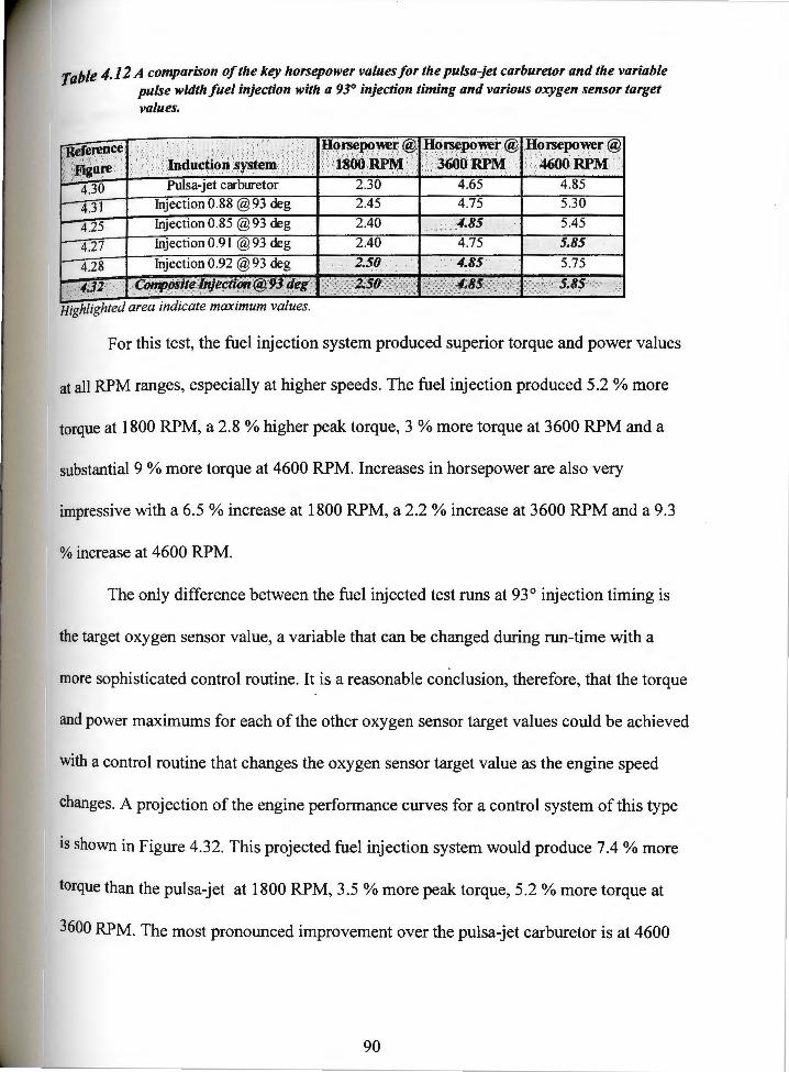
Table 4.12 A comparison of the key horsepower values/or the pulsa-jet carburetor and the variable pulse width fuel injection with a 93° injection timing and various oxygen sensor target values.

Injection 0.88 @93 deg

4.25 Injection 0.85 @93 deg 2.40

4.27 Injection 0.91 @93 deg 2.40

4.28 Injection 0.92 @93 deg

4.321111•~. ;COlppofUe fltje,~!l'1fl:@;9~4eg,~ Highlighted area indicate maximum values.

·.· . . 4.85

@ Hom;.~~r::@ . . . o() RPM: .. @'

4.85 5.30

5.45

5.85

For this test, the fuel injection system produced superior torque and power values

at all RPM ranges, especially at higher speeds. The fuel injection produced 5.2 % more

torque at 1800 RPM, a 2.8 % higher peak torque, 3 % more torque at 3600 RPM and a

substantial 9 % more torque at 4600 RPM. Increases in horsepower are also very

impressive with a 6.5 % increase at 1800 RPM, a 2.2 % increase at 3600 RPM and a 9.3

% increase at 4600 RPM.

The only difference between the fuel injected test runs at 93° injection timing is

the target oxygen sensor value, a variable that can be changed during run-time with a

more sophisticated control routine. It is a reasonable conclusion, therefore, that the torque

and power maximums for each of the other oxygen sensor target values could be achieved

with a control routine that changes the oxygen sensor target value as the engine speed

changes. A projection of the engine performance curves for a control system of this type

is shown in Figure 4.32. This projected fuel injection system would produce 7.4 % more

torque than the pulsa-jet at 1800 RPM, 3.5 % more peak torque, 5.2 % more torque at

3600 RPM. The most pronounced improvement over the pulsa-jet carburetor is at 4600

90

RPM, with the injection system producing 20.7 % more torque. Horsepower increases are

also excellent, with the projected composite injection system making 8.3 % more power

at 1800 RPM, 4.3 % more power at 3600 RPM and a huge improvement of20.6 % at

4600RPM.

91

Horsepower ·e ~ ; Torque {Ft-Lbs}

= .... N ""' ""' Ul O'I ~~iii Ul Ul O'I O'I ---l ---l 1800 n: <& = u. = u. = u.

:' ri i] 1800

2000 !! ~l 2000

2200 k t=; 2200

2400

2600 II 2600 ::c

2800 0 ~ "'I 2800 ~ fll

~ 0

= ~ "'I "O = ,.Q

"° I 11,9. 3000 0 11,9. 3000 = N = ~ n = ~ n rJJ ~ rJJ <

'Cl 3200 "'I 'Cl 3200 fll

n < n n 00 c. fll n "O c. ~ 3400

00 ~ 3400

~ "O ~

~ c. ~ ~

- 3600 c. ~ 3600

3800

4000 4000 "ti "ti s:: s::

4200 r;;- 4200 ~ Cl '-!. '-!. ~ ~

4400 it B 4400 It B .... ., ~~ ~· ~ ';:;;· s:: - "' 4600 - ~

4600 -- --~ ~ w~

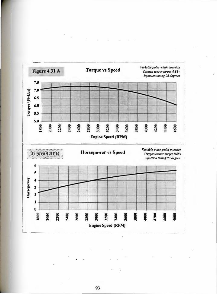
93

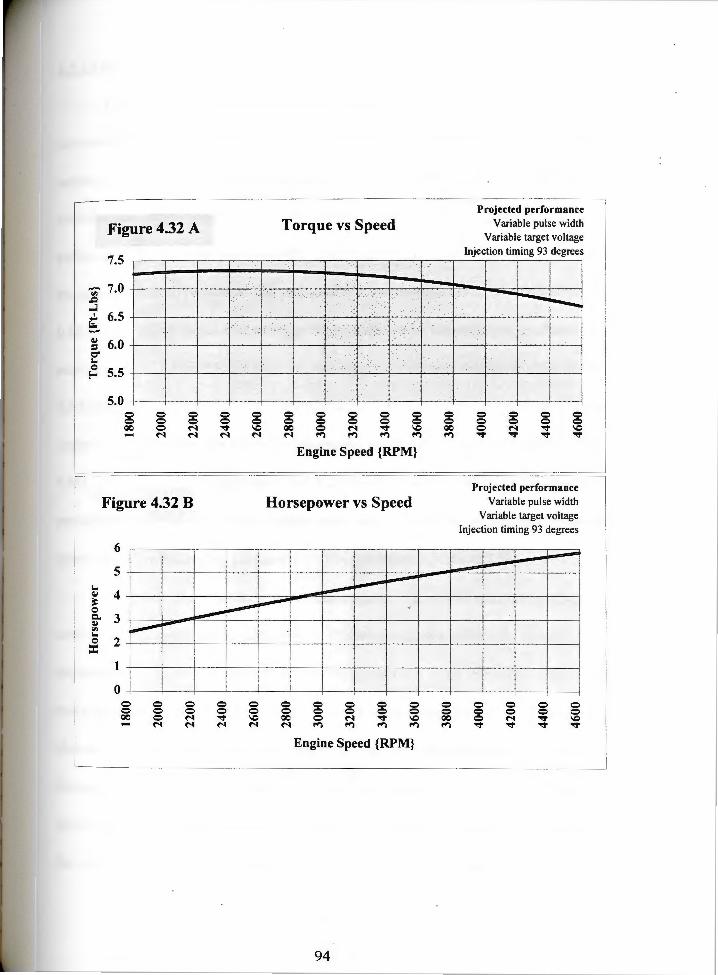
Figure 4.32 A

7.5

- 7.0 "' .&:;

....;i I 6.5 ....

i;... -~ 6.0 = I

-a' I-0 5.5 E-

5.0 0 0 0 0 0 0 0 0 QO 0 M ...,. - M M M

Figure 4.32 B

1

0 0 0 0 0 0 0 0 0 QO 0 M ...,.

M M M

Torque vs Speed

...

0 0 IC M

Engine Speed {RPM}

Horsepower vs Speed

0 0 0 0 0 0 0 0 0 0 0 0 IC QO 0 M ...,. IC M M !"') !"') !"') !"')

Engine Speed {RPM}

94

0 0 QO !"')

Projected performance Variable pulse width

Variable target voltage Injection timing 93 degrees

Projected performance Variable pulse width

Variable target voltage Injection timing 93 degrees

0 0 0 0 0 M ...,. ...,.

4 5 CONCLUSIONS ~

The electronic fuel injection system produces more torque than the stock pulsa-jet

carburetor throughout all non-racing application (1800 -- 3600 RPM) engine speed

ranges. At higher than normal engine speeds, (3600 -- 4600+ RPM) the improvements

with the fuel injection system were even more dramatic. The fuel injection system

performed better than the pulsa-jet carburetor even when subjected to the limitations of

the pulsa-jet's air to fuel ratio. The fuel injection system with a 93° injection timing and

0.88 oxygen sensor target (the average value produced by the pulsa-jet) produced 5.2 %

more torque at 1800 RPM, 2.8 % more peak torque, 3.0 % more torque at 3600 RPM, and

9.0 % more torque at 4600 RPM. An the optimum oxygen sensor target settings for each

respective speed range, the fuel injection system produced 7.4 % more torque at 1800

RPM, a 3.5 % peak torque increase, and 5.2 % more torque at 3600 RPM. The torque

production at higher than normal engine speed ranges is even more dramatic, with the

injection system producing a dramatic 20. 7 % more torque at 4600 RPM.

The pulsa-jet carburetor is an adequate system for normal engine operating

conditions, but an electronic fuel injection system is superior, especially for racing

applications. The flatter torque curve and correspondingly more linear horsepower curve

make the fuel injected engine ideal for racing. With this torque curve, other vehicle

changes like axle gearing are not as critical because the torque production does not

decrease quickly once out of a certain engine speed range. In a typical circle track racing

application, a technician would need to select a gear set that is matched to the length of

the track. A shorter track will call for higher gear ratios to enhance acceleration. The top

95

speed will be lower with higher gears, but the short track length limits the attainable high

speed. A long track will allow for higher gearing and a higher top speed. The purpose of

changing gears is to match the engine's anticipated operating speed during the race to the

operating range for peak torque production. If an engine has a very peaky torque curve,

the job of selecting gear ratios becomes more difficult and more critical to vehicle

performance. A flatter torque curve means that the vehicle is much less susceptible to

errors in gearing selection and will perform more consistently from track to track.

The feedback control system allows for more consistent control of air to fuel

ratios, especially during actual engine run-time. The carburetor must be adjusted before a

race begins, and cannot be easily altered during the course of the race. The stock pulsa-jet

carburetor can only be adjusted by replacing the orifice at the bottom of the fuel inlet

tube. This requires removal of the carburetor to gain access to the orifice. The electronic

fuel injection system allows modification of the air to fuel ratio by a computer program

change only. Once the target lambda sensor value has been selected, the feedback control

system continuously maintains the air to fuel ratio during engine operation.

4.6 SUGGESTIONS FOR FURTHER RESEARCH

Electronic fuel injection has been used on production automobiles for over 20

years. Throughout the course of those years, the electronic fuel injection systems have

continually been improved. The single cylinder fuel injection system has many aspects

that can be further investigated and improved. The object of this research was to

investigate the potential for improvements in torque and power possible with a fuel

96

injection system. The results shown in the previous sections positively demonstrate the

fuel injection system's potential. There are many other aspects to a fuel delivery system

that could be investigated. One of the most important areas of concern recently has been

pollution production. Since the air to fuel ratio can be controlled more precisely with a

fuel injection system than with a carburetor, it stands to reason that a fuel injected engine

will produce less pollution. This theory has been proven on automobile engines, where

electronic fuel injection systems produce less pollution than carbureted engines. Some of

the other general performance characteristics could also be investigated. These

characteristics include ease of starting, reliability, throttle response, cold weather

operation, part throttle operation, and idle operation. Many of these characteristics are

best tested on an engine in actual operating environments. Further refinement of the

control system, especially the implementation of a variable lambda sensor target would

serve to enhance the benefits of the electronic fuel injection system, especially in these

real world situations. Electronically controlled fuel injection timing could also be further

investigated as a performance improvement. Finally, adaptation of the controlling

computer program to a dedicated microprocessor would allow the electronic fuel

injection system to be self-contained and portable for testing in a vehicle or other piece of

equipment.

At the time of this writing, there are no fuel injection systems used on any

common application small engines. This includes 2- and 4- cycle single or twin cylinder

gasoline engines under 24 horsepower. Common applications include lawnmowers, lawn

and garden tractors, chainsaws, snowblowers, leaf vacuums and blowers, go-carts, water

97

pumps, generators, and many other items. There are a number of reasons that electronic

fuel injection technology has not been brought to market for these products. The first and

most dominant reason is cost. Electronic fuel injection systems are not yet cost effective

enough to be marketable. When pollution control requirements get too strict for

carbureted small engines to meet (as they did with carbureted automobile engines) the

increased cost of fuel injection will no longer be a factor.

Another problem that could plague production fuel injection systems is the

seasonal use that most of the equipment gets. Snowblowers sit unused for 7 or more

months each year. Lawnmowers remain unused through the late fall, winter, and into the

spring. Chainsaws typically only see use in the fall and after heavy storms. Leaf blowers

are only used one month per year. Stand-by generators can be the worst, sometimes going

years without being run. Sitting without being used can cause a number of fuel system

maladies. Water gets into the fuel system and rusts the gas tank and blocks fuel lines. The

water itself can prevent the engine from starting or running properly. Gasoline loses its

volatility and turns to a varnish-like residue that would clog fuel lines, fuel filters and fuel

injectors. All of these problems already occur with carbureted engines, however, so fuel

injection systems would not create a problem that did not previously exist. Simple

maintenance procedures will prevent these problems altogether, but few consumers take

the time to perform these procedures.

98

REFERENCES

[l] Domestic Fuel Injection Manual, Mitchell International, p.vii, 1993

[2] Urich, Mike and Fisher, Bill, Holley Carburetors, Manifolds, and Fuel Injection, The

Berkley Publishing Group, New York, pp.192-193, 1994

[3] Briggs & Stratton Service and Repair Instructions, Briggs & Stratton Corporation,

Milwaukee, WI, pp.7-12, 1984

[4] Domestic Fuel Injection Manual, Mitchell International, p.vii, 1993

[5] Domestic Fuel Injection Manual, Mitchell International, p.vii, 1993

[6] Pheil, Don, and Haynes, John H., The Haynes Fuel Injection Manual, Haynes North

America, pp.7-9, 1986

[7] "Electronic Fuel Injection." Machine Design v62 August 23, 1990: 82-3

[8] Pheil, Don, and Haynes, John H., The Haynes Fuel Injection Manual, Haynes North

America, p.11-22, 1986

[9] Wood's Industrial Power Transmission Products, T.B. Wood's Sons Company,

Chambersburg, PA, p.40M-2, 1992

[10) ADJ JOO User's Manual, Real Time Devices, Inc., State College, PA, p.4-1 , 1990

[11) Snap-On General Motors Reference Manual, Balco, Inc., pp.66-68, 1991

[12] Briggs & Stratton Service and Repair Instructions, Briggs & Stratton Corporation,

Milwaukee, WI, p.26, 1984

99

BIBLIOGRAPHY

ADI I 00 User's Manual, Real Time Devices, Inc., State College, PA, 1990

Aitken, Peter, and Jones, Bradley, Teach YourselfC in 21 Days, SAMS Publishing, 1992

Austlander, David M. and Tham, Cheng H., Real-Time Software for Control: Program

Examples in C, Prentice Hall, 1990

Bollinger, John G. and Duffie, Neil A., Computer Control of Machines and Processes,

Addison-Wesley Publishing Company, 1988

Briggs & Stratton Service Engine Specifications and Price List, Briggs & Stratton

Corporation, 1994

Briggs & Stratton Service and Repair Instructions, Briggs & Stratton Corporation,

Milwaukee, WI, 1984

Domestic Fuel Injection Manual, Mitchell International, 1993

"Electronic Fuel Injection." Machine Design v62 August 23, 1990: 82-3

Heywood, John B., Internal Combustion Engine Fundamentals, McGraw-Hill, Inc., New

York, 1988

Internal Combustion Engines Analysis and Practice, International Textbook Company,

1950

Lafore, Robert, The Waite Group's Microsoft C Programming for the PC, Howard W.

Sams and Company, 1990

Pheil, Don, and Haynes, John H., The Haynes Fuel Injection Manual, Haynes North

America, 1986

100

Snap-On General Motors Reference Manual, Balco, Inc., 1991

Stone, Richard, Introduction to Internal Combustion Engines, Society of Automotive

Engineers, Inc., 1993

The Internal Combustion Engine in Theory and Practice, The M.I.T. Press, Cambridge,

MA, 1966

Urich, Mike and Fisher, Bill, Holley Carburetors, Manifolds, and Fuel Injection, The

Berkley Publishing Group, New York, 1994

Vizard, David, How to Build Horsepower Volume 1, S-A Design Books, Brea, California,

1990

Wood's Industrial Power Transmission Products, T.B. Wood's Sons Company,

Chambersburg, PA, p.40M-2, 1992

101