1

Application of a new spatial computable general equilibrium model

for assessing strategic transport and land use development options in

London and surrounding regions

by Jie Zhu

*, Ying Jin

** and Marcial Echenique

***

The Martin Centre for Architectural and Urban Studies,

University of Cambridge

Paper to be presented to ERSA congress 2012, August 2012, Bratislava

ABSTRACT: This paper reports the application of a new spatial computable

general equilibrium (SCGE) model at the city region level for analyzing the wider

economic impacts of strategic transport and land use development options. We start

from a static computable general equilibrium model for an open economy, and extend

it to incorporate (1) agglomeration effects on productivity that ariseing from

urbanization and transport improvements, (2) labour mobility across the study area

with both commuting and migration, (3) short run and long run counterfactual

equilibrium to allow for different rates of change in economic activities and

residential location, (4) land as an explicit factor input to production, and (5) concave

transport cost functions with respect to travel distance that are consistent with realistic

transport costs. These extensions are built on the Dixit-Stiglitz model of monopolistic

competition among producers, random utility theory of residents’ behaviour, the

concept of spatial economic mass, interregional trade pooling, and the Armington

specification regarding product varieties. Data from London and surrounding regions

is used to calibrate and validate the model. We report its applications in studying a

new high speed rail link, dualing of a rural highway, and increased suburban and

exurban land supply for business use. The model results obtained are in line with

theoretical expectations and provide new quantification of the costs and benefits that

may feed into the assessment of those strategies. All results reported in this paper are

provisional although no major changes are expected.

JEL Classification: C68, F12, F16, F17, O18, R13, R42

Key words: computable general equilibrium models; land use and transport modelling,

agglomeration; land; infrastructure investment appraisal

* mail to: jz286@cam.ac.uk ** mail to: yj242@cam.ac.uk *** mail to: me15@cam.ac.uk 1 See Appendix D for derivation

2

1. Introduction

This paper reports the application of a new spatial computable general equilibrium

(SCGE) model which aims to assess city region level development options,

particularly those related to land use and transport strategies. Our model is a further

development and implementation of the models of Bröcker[2]

, Bröcker[3]

, Bröcker et

al.[5]

, Bröcker and Schneider[4]

and Schneider[13]

. The plan of the paper is as follows.

In section 2, we outline the basic structure of the model. In section 3 and 4, we discuss

data and solve the model, then interpret the model simulation results. Finally, in

section 5, we draw the main conclusions from the applications. In this paper, we have

included the main formulae of the models but not the detailed derivations. Detailed

explanation and verification of the equations are found in draft Chapter 3 of Jie Zhu's

dissertation (forthcoming) which is available upon request.

2. Model Structure

Our model is a static computable general equilibrium model for the UK as an open

economy with geographical disaggregation of production and residential locations at

the subregional level. The model consists of 3 broad industry sectors (primary,

secondary and tertiary), 2 foreign country groups (EU and non-EU) and 62 UK zones

with the majority representing London and its surrounding regions. For each UK zone,

the model classifies economic activities into four broad sectors: production carried out

by firms of the 3 types of industries, with the total number of firms being determined

endogenously; a transport agent, who has an Armington preference[1]

on products

from different origins and is responsible for aggregating commodities from all

relevant zones in a pool[11]

, from where deliveries are made to both intermediate and

final consumers; final demand by households, who earn income by selling primary

production factors (labour, capital and land) to firms then spend the income on pool

goods, subject to their perception of consumption utility; and an export agent whose

behaviour is analogous to the transport agent for commodities exported from the UK.

Figure 1 shows the circular flow of the model. A brief description of the model

follows from Section 2.1 to 2.5.

3

Figure 1. Overview of the model structure

Production Households

Transport Agents

Export Agents Foreign countries

Primary factors Factor payments

Outputs Pool goods

Outputs Pool goods

Imports

2.1 Production

Following Bröcker[3]

and Bröcker et al.[5]

, we design the firms' production process

with two stages as shown in Figure 2 and Figure 3. In the first stage, the firms produce

a homogenous raw output I by means of a two level NCES linear-homogenous

production technology under perfect competition with constant returns to scale, using

intermediate inputs i=1,…,I, taken from the pool in zone s at the upper level, and

using primary factor inputs k=1,…,K at the lower level. To keep the model simple, it

is assumed that within each sector firms in all zones produce using a same Leontief

technology at the upper level and a zonal specific external increasing returns to scale

CES technology at the lower level. According to Shephard’s lemma,

cost-minimization behaviour yields the technology coefficients in terms of

intermediate goods and the value-added coefficients as the first derivatives of the

nested CES unit-cost functions, j

cf , with respect to individual prices.

,

,

,

( , ; , )j s s j j s

ij s ij

i s

cf q wa

q

α γα

∂= =

∂ (1)

(1 ), ,(1 ),

11

, ,

, , , ,

1,,

1

( , ; , )( ( ))

j P j Pj P

Kj s s j j s kj s

kj s k s k s kj sKkk s

kj s

k

cf q wc w w

w

σ σσα γ γγ

γ

− −−−

=

=

∂= =

∂∑

∑ (2)

where ij

α and ,kj sγ are known as position parameters. ,ij s

a and ,kj sc are the

intermediate and value added coefficients in zone s. ,i sq and ,k s

w are the prices for

pool goods and primary factors. Our external increasing returns to scale effect is

assumed to be Hicks neutral here and is measured with spatial economic mass or

4

effective density[8]

which is formulated as

( )s r

s rs

rss sr

LD LDED

d d

≠

= +∑ (3)

where s

LD and r

LD are the total labour demand at zone s and r; ss

d is the

intrazonal distance within zone s; and sr

d is the interzonal distance between zone s

and r. This means that ,kj sγ takes the form of:

,

, ( ) j EDskj s kj

B

ED

ED

σγ γ

−= (4)

where position parameter kj

γ is associated with the national average technology used

to produce value added; BED is a national base level effective density to be chosen

for normalization and can be set equal to one arbitrary zone's s

ED ; ,j EDσ is the

elasticity of effective density on productivity for sector j.

In the second stage, the firm takes the raw output as the only input required to produce

varieties of final output under monopolistic competition in the Dixit-Stiglitz[6]

style

and a fixed amount of that raw output per variety plus a constant marginal amount per

unit of final output is required for producing final goods. Under this specification,

each variety is monopolistically supplied by one firm. If the price is a fixed mark-up

over marginal costs and profits are driven to zero by free market entry, then output per

variety is also fixed so the total final output of diversified goods is proportional to the

amount of raw output used for producing them. With an appropriate choice of units

the factor of proportionality can be chosen to be unity, such that the zonal raw output

quantity ,i rX is the same as the zonal final diversified output '

,i rX , and the raw

output price ,i rp equals the final diversified output price '

,i rp . The composite of

zonal varieties therefore has the price1

,

,

1

11,

, ,

,

( )i r

i ri r

i r i r

i B

Xp

X

εε

υ−

− =

(5)

where ,i BX is the total supply for sector i at national level in the base year

benchmark . ,i rε is the elasticity of substitution between varieties for sector i within

each production origin r and is assumed to be the same across all domestic zones in

5

the model.

We assume foreign country producers also use raw output to produce final goods

under Dixit-Stiglitz type of monopolistic competition. Similarly, the price of

composite of varieties for sector i from foreign country z takes the form of

,

,

1

11,

, ,

,

( )i z

i zi z

i z Mi z

i B

Mp

X

εε

υ−

− =

(6)

where ,Mi zp is the import price for sector i from foreign country z. For simplicity,

,i zε , the elasticity of substitution between varieties for sector i within each foreign

country z is also assumed to be the same across all foreign countries.

Figure 2. Nested Leontief-CES production functions

Raw output prices

LEONTIEF

…

i=1 i=I CES

Intermediate goods prices

k=1 k=K

…

Primary factor prices

,j sp

,i sq

,k sw

,j pσ

Figure 3. Production of final diversified output

marginal cost

average cost

output per variety

output price

6

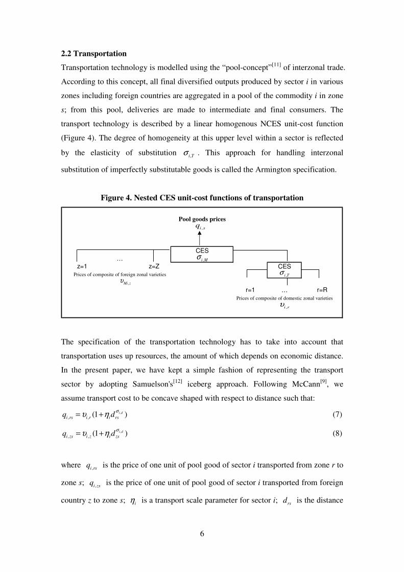
2.2 Transportation

Transportation technology is modelled using the “pool-concept”[11]

of interzonal trade.

According to this concept, all final diversified outputs produced by sector i in various

zones including foreign countries are aggregated in a pool of the commodity i in zone

s; from this pool, deliveries are made to intermediate and final consumers. The

transport technology is described by a linear homogenous NCES unit-cost function

(Figure 4). The degree of homogeneity at this upper level within a sector is reflected

by the elasticity of substitution ,i Tσ . This approach for handling interzonal

substitution of imperfectly substitutable goods is called the Armington specification.

Figure 4. Nested CES unit-cost functions of transportation

Pool goods prices

CES

…

z=1 z=Z CES

Prices of composite of foreign zonal varieties

r=1 … r=R

Prices of composite of domestic zonal varieties

,i sq

,Mi zυ

,i rυ

,i Mσ

,i Tσ

The specification of the transportation technology has to take into account that

transportation uses up resources, the amount of which depends on economic distance.

In the present paper, we have kept a simple fashion of representing the transport

sector by adopting Samuelson's[12]

iceberg approach. Following McCann[9]

, we

assume transport cost to be concave shaped with respect to distance such that:

,

, , (1 )i d

i rs i r i rsq dσ

υ η= + (7)

,

, , (1 )i d

i zs i z i zsq dσ

υ η= + (8)

where ,i rsq is the price of one unit of pool good of sector i transported from zone r to

zone s; ,i zsq is the price of one unit of pool good of sector i transported from foreign

country z to zone s; i

η is a transport scale parameter for sector i; rs

d is the distance

7

between zone r and s and ,i dσ is a transport shape parameter with ,0 1

i dσ< < to

incorporate transport economies of scale. Therefore, the pool good price of sector i in

zone s takes the form of

,, , , ,

, ,

1

1(1 ) (1 ),

, , , , ,

1 1 1,

( , ; , )

( ) ( (1 )) ( )i M

i M i z i d i M

i s i s i i Mi

Z R Zi z

i ir T Mi z i zs iz M i r Mi z

z r zi B

q ct p p

Mp p d

X

σσ π σ σ

ϑ ϑ

φ η φ ϑ ϑ−

− −

= = =

= =

= + + +

∑ ∑ ∑ (9)

with

(1 ),, , ,

,,1

, .

, , , ,

1 1 1 1

1

(1 ), ,

,

1 ,,

1

, ,

, ,

, ,

, and

( ) ( )

( ( ) ( (1 )) )

1 1,

1 1

i Ti r i d i T

R

i rMi zr

ir T iz MR Z R Z

i r Mi z i r Mi z

r z r z

Ri r i r

i i r i rs Rr i B

i r

r

i T i M

i r i z

i r i z

Xp p d

X

σπ σ σ

ϑϑ

φ φ

ϑ ϑ ϑ ϑ

ϑη

ϑ

σ σπ π

ε ε

−

=

= = = =

−

=

=

= =

+ +

= +

− −= =

− −

∑

∑ ∑ ∑ ∑

∑∑

where ,i Mσ is the sector specific elasticity of substitution between domestic and

foreign goods. ,i rϑ and ,Mi zϑ are sector specific Armington preference factors for

domestic goods produced in zone r and imported goods from foreign country z. It is

assumed that both ,i rϑ and ,Mi zϑ only varies over origin zones but not over

destination zones; the competition parameter ,i rπ and ,i z

π controls the position of

locational and sectoral specific market form between perfect competition ( 0π = ) and

pure Dixit-Stiglitz ( 1π = ) monopolistic competition for domestic zones and foreign

countries respectively. By introducing π , we introduce a supply market size effect on

pool goods price ,i sq . As π goes to zero, the supply market size effect vanishes and

we approach perfect competition. For 1i i

ε σ> > , we have 1π < .

2.3 Households

On the households side, each zone s consists of a set of homogenous households and

each household produces one labour. Following Thissen et al[15]

, we specify a

multiplicative utility (s

u ) function (Figure 5) consisting of utilities derived from both

consumption ,c su and living ,l s

u . One the one hand, the households in zone s earn its

8

income by selling its production factors to firms. For distribution of income, we

assume wage income follows commuters and is equally redistributed among

households within each residential zone while capital and land rental are modelled as

a national dividend. The households spend their full income on the consumption of

pool goods i=1,…,I and derive utility from this consumption. This part of the

household behaviour is described by a linear-homogeneous utility function and a CES

expenditure function. On the other hand, the households also obtain utility from living

in a zone and this zone related utility is specified by a logarithmic decreasing returns

function including zonal housing stock (s

H ), zonal labour supply (s

L ) and living

attractiveness constant s

F according to equation (11). To release the restriction on

interzonal labour mobility of commuting and migration, we define a commuting

utility ,com sru with a log linear function

[10] consisting of workplace and residential

wages ( 1,rw and 1,sw ) , commuting cost2 (

rsdφ ) and zonal pair specific commuting

constant sr

v inside of a multinomial logit function, and adopt the utility equalization

assumption to classify three types of equilibrium including: 1) Benchmark; 2)

counterfactual short run (SR); and 3) counterfactual long run (LR) where both

benchmark and LR represent a respective situation of utility equalization and labour

migration is only allowed in LR.

, ,s c s l su u u= (10)

, ln( )sl s s

s

Hu F

L= (11)

, 1, 1,ln ln ln( ) lncom sr r s sr sr sr

u w w d vφ ς= − − − + (12)

where sr

ς is a double exponential stochastic random term capturing individual

heterogeneity in commuting preferences.

2 The commuting cost is assumed to be internal to labour as all household's income is fully spent on consumption.

9

Figure 5. Household's personal utility function

Personal utility

Multiplicative

Utility (consumption) Utility (living)

CES Decreasing

returns

i=1 … i=I Living attraction Housing

pool goods

su

,c su ,l s

u

sF sH

Hσ

Figure 6: A two-level export demand function

Total export demand

Export prices

CES

r=1 … r=R

Prices of composite of domestic zonal varieties

,i rυ

,Ei zq

,i ze

,i Tσ

2.4 Foreign trade

The apportionment of exports and imports to domestic zones follows the same

principles as inter-zonal trade between domestic zones. Import supply ,i zM is

assumed to be perfectly elastic with ,Mi zp exogenously specified. Total export

demand ,i ze is determined by a constant elasticity of export demand function

according to export prices Ei,z

q and the export agent's behaviour is assumed to be

similar to the domestic transport agents and the export activity is carried out by means

of a CES linear-homogenous technology (Figure 6).

10

2.5 Equilibrium conditions

Equilibrium is characterized by a set of goods and factor prices for which excess

demands for both goods and factors vanish. The set of equilibrium conditions consists

of

, , , , , , ,

1 1 1

( )S J Z

i r i rs i s ij s j s Ei rz i z

s j z

X t FD a X t e= = =

= + +∑ ∑ ∑ (13)

, , , , ,

1 1

( )S J

i z Mi zs i s ij s j s

s j

M t FD a X= =

= +∑ ∑ (14)

, , , ,

1 1

( )S I

k rs k r i r ki r

s i

f fd X c= =

= =∑ ∑w (15)

with

, , ,

, , ,

, , ,

, ,i s Ei z i s

i rs Ei rz Mi zs

i r i r Mi z

q q qt t t

p p p

∂ ∂ ∂= = =

∂ ∂ ∂

where ,i rst , ,Ei rzt and ,Mi zst are domestic, export and import trade coefficients; ,i sd

is the sector specific zonal final demand; , ( )k r

fd w denotes factor demand given

factor price vector w and ,k rsf denotes factor supply flow.

3. Data and Model Calibration

The model is calibrated based on the following data sources:

• A Social Accounting Matrix (SAM) for the UK (OECD,2000)

• Employment data by sector at NUTS4 level (ABI, 2000)

• Factor prices3 (ASHE, 2000 and VOA,2000)

• Crow-fly distance matrix (UKBORDERS,2000)

• Labour commuting matrix (CENSUS, 2001)

The calibration and solving techniques follow Scheneider [13]

with extension to labour

commuting and migration modelling and is programmed within MATLAB. The

calibration is accomplished such that the values of modelled values of interindustry

flows and primary inputs, when aggregated over model zones for the benchmark

equilibrium, exactly add up to the values observed in the SAM. When calibrating

3 Capital price is set to 1 everywhere.

11

benchmark equilibrium, external information is required for fixing those exogenous

parameters (e.g. elasticity of substitution and transport rates). So far, we have

consulted an extensive literature where a majority comes from the UK sources and all

remained parameters are experimental based on regional available evidence. Those

parameter values are reported in Table 1 and 2. The main outputs obtained from

calibration contain position parameters as well as estimated capital and land stocks,

both of which can be used to define policy changes and simulate counterfactual

equilibriums. We specify full employment of labour and land due to the assumption of

perfect price flexibility4 and the general solving algorithm for finding updated factor

prices to clear factor markets in the respective counterfactual equilibrium is based on

the Levenberg-Marquardt method as offered by MATLAB's optimization toolbox as

an alternative to the common Newton-Raphson method.

Table 1: Transport and competition parameter values

Industry Sector Scale Parameter

iη (per

km) Shape Parameter ,i d

σ

Primary 0.0019 0.75

Secondary 0.0014 0.75

Tertiary 0.0014 0.75

4 Capital price is fixed from base year benchmark and capital supply is assumed to be perfectly elastic.

12

Table 2: Main exogenous parameter values specified in the model

Elasticity of substitution

Production Transport Import Consumption

Concentration

parameter for

commuting Type

,j pσ ,i T

σ ,i Mσ

Hσ

comλ

Primary 0.3 6.0 4.0 - -

Secondary 0.4 6.0 4.0 - -

Tertiary 0.8 6.0 4.0 - -

Household - - - 0.5 2.0

Price elasticity of export demand Elasticity of productivity with

respect to effective density EU excluding UK

ROW (Rest of

the World) Type

,i EDσ ,i z

ζ ,i zζ

Primary 0.1 1.0 1.0

Secondary 0.1 1.0 1.0

Tertiary 0.2 1.2 1.2

Competition parameter

UK EU excluding UK ROW Type

,i rπ ,i z

π ,i zπ

Primary 0.10 0.10 0.10

Secondary 0.30 0.30 0.30

Tertiary 0.50 0.50 0.50

13

4. Results and Discussion

4.1 Base year benchmark

For the base year (2000) benchmark model, we first present one of the distinctive

features in our model, namely the spatial distribution of effective density as calculated

by equation (3). As shown in Figure 7, such a kind of distribution reflects the pattern

of the London-centric urban agglomeration.

Because zonal factor stock other than labour is calibrated in the model, we make a

comparison on the distribution of zonal business land stock between the modelled and

the observed. Figure 8 below shows a good match between the two.

Figure 7: Spatial distribution of effective density, Benchmark Model for 2000

14

Figure 8: Zonal share of business land, modelled versus observed, base year

benchmark

R2 = 0.9962

0.00%

2.00%

4.00%

6.00%

8.00%

10.00%

12.00%

14.00%

16.00%

18.00%

0.00% 2.00% 4.00% 6.00% 8.00% 10.00% 12.00% 14.00% 16.00% 18.00%

Modelled

Ob

serv

ed

*The percentage distribution above are calculated based on the exclusion of Wales, Scotland and

Northern Ireland because observed business land stock for those regions are not available from

Generalised Land Use Database (2001) in the UK.

Figure 9: Summary of counterfactual equilibrium scenarios

15

4.2 Overview of the simulation scenarios

Before introducing the counterfactual equilibrium scenarios, we first classify two sets

of benchmark equilibrium: base year and future year. Our base year benchmark

equilibrium is calibrated for the year 2000, whereas the future year (2030) benchmark

is obtained from the base year model through a long run counterfactual simulation run

by applying growth factors on exogenous variables including total labour supply,

dwellings stock and export demand while assuming all other inputs (such as zonal

business land supply) and calibrated parameters from the base year benchmark remain

constant. We then carry out three further counterfactual scenario runs from the 2030

benchmark model. These scenarios (as shown in Figure 9 above) are: A) the first stage

of the proposed UK High Speed 2 (HS2) railway project between central London and

Birmingham; B) dualing the 14 km single carriageway section of the A11 trunk road

between Mildenhall and Thetford in the County of Norfolk to the Northeast of

London; and C) business land supply to increase by 20% for London’s Green Belt

North West. The transport schemes are represented by readjusting the distance matrix

used by the model for each type of activity as appropriate. For instance, the High

Speed Rail project in Scenario A causes economic distances to change for the tertiary

sector (because of business travel), but not for the primary and secondary industry

sectors.

We perform a comparative analysis first on the results of future year benchmark with

respect to the base year benchmark for 2000, and then on the counterfactual scenarios

with respect to the future year benchmark for 2030. The model outputs four main

types of variables: quantities (production, pool goods, factors, interzonal trade flows,

final demands, imports and exports), prices (production prices, pool goods prices,

factor prices), values (production, final demand, imports and exports, factor income)

and the utilities (personal utility and commuting utility). Our analysis here is focused

on the values of production, imports and exports, factor demand and price, as well as

personal utility. All results are measured as percentage changes from the respective

benchmark equilibrium.

16

4.3 Future year benchmark

As mentioned above, our future year benchmark for 2030 is not calibrated but derived

from a base year counterfactual long run. Therefore, it is equivalent to an export

demand driven scenario and the results at national level in Table 4 below can be

understood as follows. The exogenously specified growth of exports leads to

increased demand on both commodity markets and factor markets. Given those

specified factor supply changes and due to the assumption of perfect price flexibility,

the new equilibrium factor prices of labour and land indicates a rise in order to clear

their markets. This increase of factor prices has two consequences. First, it leads to an

increase of domestic production prices and therefore a decline of relative import

prices (due to import prices being fixed from the base year). This in turn leads to an

increase of imports, which dampens the increase on pool goods prices due to increase

on domestic production prices. Second, the increased factor stock and their prices lead

to an increase of personal income. Our results show that the increase on national

average personal income outweighs the increase on price index5 and hence leads to

an increase of personal utility from consumption. This part of the utility increase is

combined with the change of utility derived from living and finally leads to a net

increase of national average personal utility.

Table 4: Relative changes (%) from base year benchmark (2000), future year

benchmark (2030)

Type Sector Relative Changes (%) for UK as a whole

Primary 22.0

Secondary 26.3 Production

value Tertiary 29.7

Primary 14.7

Secondary 16.9 Production

price Tertiary 19.7

Primary 10.3

Secondary 6.4 Pool goods

price Tertiary 13.6

Primary 129.0

Secondary 157.0 Export value

Tertiary 191.8

5 Price index is defined as the expenditure needed to reach one unit of utility. This is also know as the zonal price

index[2]. In this model, a national average price index can be calculated by summing up all zonal price indices

weighted with zonal personal utility from consumption.

17

Type Sector Relative Changes (%) for UK as a whole

Primary 117.6

Secondary 124.7 Import value

Tertiary 422.4

Labour 17.0 Factor demand

Capital 49.9

Labour 44.2 Factor price

Land 80.8

Personal income 39.5

Price index 10.8

Personal utility 25.6

4.4 Counterfactual scenario analysis

For all three counterfactual scenarios, it should be noted that the following three

causal chain effects together with the interplay between all markets in the economy

determine the new equilibrium results. The first is a direct effect resulting from the

change of transport cost or factor endowment, which generates a shock on both

commodity markets and factor markets. The second is an indirect effect resulting from

an increase in zonal production, which generates a stronger supply market size effect

on pool goods price and its related trade and therefore also leads to secondary shocks.

The third effect is related to productivity improvements as a result of a change in

effective density, which again generates some additional shocks. Those three causal

chain effects are valid across all sectors and all zones in the model. Obviously, the

magnitude of the effects also depends on underlying assumptions such as exogenously

given parameters and elasticities.

As seen from Table 5, variations on the level of sector production changes are

predicted across all regions and scenarios. Those variations, either positive or negative,

are fully determined by the three causal chain effects, the relative changes on factor

prices and the inter-industry relations stated in the SAM table. In general, those

regions that directly benefit from the shocks show an increase in total production and

labour demand whereas most other regions show various degrees of reductions

because they suffer from zonal excess supply of factor inputs. In order to pinpoint

these effects and examine them in detail, we have deliberately chosen simple

scenarios where the directly affected areas can be clearly identified: the transport

improvement in Scenario A only affects the two ends of the new transport link,

18

whereas the business land supply increase under Scenario C is only applied to one

zone. As expected, for all scenarios those zones that directly benefit from the shocks

show an increase in personal utility in the short run, which then induces a net inflow

of migrants in the long run.

Table 5: Relative changes (%) from future year benchmark at regional Level

Short Run Long Run

Personal Utility Production Value Labour Demand Labour Migration

Region\Scenario A B C A B C A B C A B C

Central London 0.09 0.004 0.02 0.23 0.00 -0.16 0.20 0.00 -0.18 0.09 0.00 0.00

Inner London 0.09 0.004 0.02 0.23 0.00 -0.09 0.20 0.00 -0.09 0.09 0.00 -0.02

Outer London 0.07 0.005 0.03 -0.14 0.00 -0.08 -0.15 0.00 -0.10 -0.01 0.00 0.03

Green Belt 0.04 0.005 0.17 -0.16 0.01 1.69 -0.18 0.00 1.47 -0.12 0.00 0.58

Urban East 0.04 0.022 0.09 -0.16 0.07 -0.09 -0.18 0.07 -0.13 -0.14 0.07 0.26

Urban South East 0.03 0.005 0.03 -0.18 0.00 -0.05 -0.20 0.00 -0.06 -0.16 0.00 0.03

Rural East 0.03 0.071 0.05 -0.14 0.26 -0.02 -0.17 0.27 -0.03 -0.16 0.23 0.14

Rural South East 0.03 0.005 0.02 -0.16 0.00 -0.03 -0.19 0.00 -0.04 -0.18 0.00 0.00

South West 0.02 0.005 0.00 -0.13 0.00 -0.06 -0.16 -0.01 -0.07 -0.15 -0.01 -0.06

East Midlands 0.04 0.002 0.01 -0.10 -0.01 -0.07 -0.13 -0.02 -0.08 -0.10 -0.01 -0.06

West Midlands 0.39 0.002 0.00 1.53 -0.02 -0.08 1.31 -0.02 -0.08 1.24 -0.02 -0.08

REST OF THE

UK 0.02 0.001 0.00 -0.13 -0.02 -0.10 -0.17 -0.02 -0.11 -0.16 -0.02 -0.10

UK 0.067 0.006 0.023 0.054 0.003 0.028 - - - - - -

4.5 Comparison with perfect competition and homogenous productivity

In this model, we have introduced effects of both external increasing returns to scale

(i.e. urban agglomeration) and Dixit Stiglitz monopolistic competition for firms (i.e.

product varieties). To isolate their effects on counterfactual scenario results, we have

recalibrated a set of alternative base year benchmarks by excluding those model

features as defined in Table 6 below. This is equivalent to set the elasticity of

productivity with respect economic mass ,i EDσ or competition parameters ,i r

π and

,i zπ to zero and basically leaves all firms to operate under constant returns to scale,

no product variety or both, which are the typical assumptions held by most traditional

LUTI (Land Use and Transport Interaction) and SCGE models. We then also derive a

19

corresponding future year benchmark with the same growth factors and rerun scenario

A, B and C for the long run counterfactual equilibrium. Therefore, we would expect

such change of specifications would provide us a good understanding of those effects'

influence on the magnitude of the model results.

Table 6: Inclusion of agglomeration and zonal variety effects for additional runs

Run 1a 1b 2 3a 3b 4

Agglomeration effect Yes Yes Yes No No No

Zonal variety effect wih zonal total

number of variety ,i rn specified as

, ,/i r i B

X X

Yes - No Yes - No

Zonal variety effect wih zonal total

number of variety ,i rn specified as

,i rX

- Yes No - Yes No

Table 7 below shows the net differences in total production values at regional level

between the long run counterfactuals and the future year benchmark for each

respective run. The results show models that do not consider urban agglomeration and

product variety effects tend to report much lower output increases in areas directly

affected by the policy interventions, and at the same time report lower output

decreases in the rest of the study area.

In this model, we have taken Tavassy et.al (2002) [15]

's suggestion to define the zonal

number of varieties ,i rn as its share of zonal production in the production of all

varieties within a sector in the base year. To see the influence of this specification on

the model results, we reset , ,i r i rχ ε equal to one as an alternative and this basically

leaves the zonal number of varieties being directly equal to the total zonal raw output

,i rX . The result differences between run 1a and 1b, as well as run 3a and 3b indicate

that a lower level specification for the zonal number of varieties from the base year

could generate a stronger impact on the zonal output for both directly affected and

indirectly affected regions, given the same policy interventions. This is because the

supply market size effect takes a concave shape due to the specification of

20

competition parameters between 0 and 1.

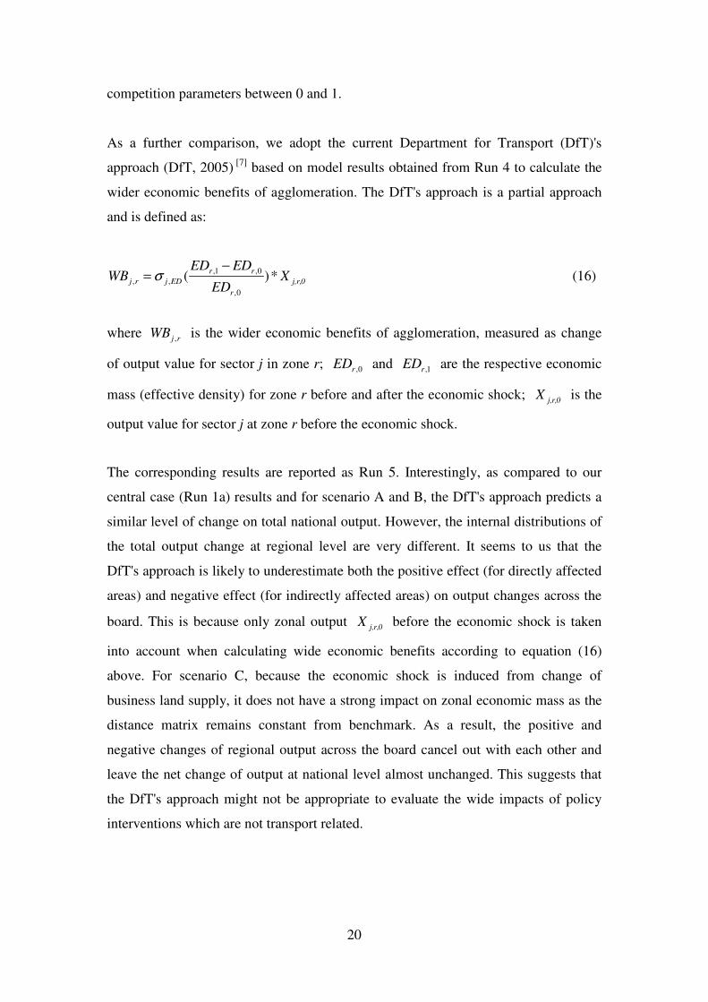
As a further comparison, we adopt the current Department for Transport (DfT)'s

approach (DfT, 2005) [7]

based on model results obtained from Run 4 to calculate the

wider economic benefits of agglomeration. The DfT's approach is a partial approach

and is defined as:

,1 ,0

, ,

,0

( )*r r

j r j ED j,r,0

r

ED EDWB X

EDσ

−= (16)

where ,j rWB is the wider economic benefits of agglomeration, measured as change

of output value for sector j in zone r; ,0rED and ,1r

ED are the respective economic

mass (effective density) for zone r before and after the economic shock; j,r,0

X is the

output value for sector j at zone r before the economic shock.

The corresponding results are reported as Run 5. Interestingly, as compared to our

central case (Run 1a) results and for scenario A and B, the DfT's approach predicts a

similar level of change on total national output. However, the internal distributions of

the total output change at regional level are very different. It seems to us that the

DfT's approach is likely to underestimate both the positive effect (for directly affected

areas) and negative effect (for indirectly affected areas) on output changes across the

board. This is because only zonal output j,r,0

X before the economic shock is taken

into account when calculating wide economic benefits according to equation (16)

above. For scenario C, because the economic shock is induced from change of

business land supply, it does not have a strong impact on zonal economic mass as the

distance matrix remains constant from benchmark. As a result, the positive and

negative changes of regional output across the board cancel out with each other and

leave the net change of output at national level almost unchanged. This suggests that

the DfT's approach might not be appropriate to evaluate the wide impacts of policy

interventions which are not transport related.

21

Table 7: Net differences on modelled total production value from future year

benchmarks for additional runs, scenario A, B and C

Region\Run** 1a 1b 2 3a 3b 4 5

Central London 320 291 224 187 140 140 71

Inner London 373 327 262 222 157 160 88

Outer London -255 -206 -169 -36 -55 -43 8

Green Belt -280 -153 -164 -43 -32 -41 3

Urban East -164 -89 -94 -26 -18 -23 1

Urban South East -215 -108 -120 -35 -21 -30 0

Rural East -123 -58 -67 -23 -13 -18 0

Rural South East -257 -121 -143 -46 -25 -38 1

South West -257 -138 -159 -69 -37 -52 1

East Midlands -187 -118 -122 -56 -30 -42 1

West Midlands 3854 2347 2368 414 239 311 1018

ROUK -1304 -692 -777 -341 -172 -244 -2

UK 1504 1282 1039 147 132 79 1190

Region\Run** 1a 1b 2 3a 3b 4 5

Central London -3 -4 -1 4 3 3 2

Inner London -1 1 1 2 4 2 3

Outer London 5 7 5 4 4 3 4

Green Belt 10 10 8 3 4 3 6

Urban East 74 33 48 19 1 14 19

Urban South East 4 4 3 2 2 1 3

Rural East 233 153 161 108 71 80 47

Rural South East 6 5 4 2 2 2 4

South West -9 -2 -4 -1 1 0 3

East Midlands -28 -16 -18 -14 -8 -10 -1

West Midlands -43 -21 -25 -18 -9 -13 -1

ROUK -170 -84 -103 -81 -40 -53 -5

UK 77 87 79 31 34 33 85

Region\Run** 1a 1b 2 3a 3b 4 5

Central London -223 -260 -122 -142 -163 -92 -8

Inner London -143 -166 -84 -108 -112 -72 -3

Outer London -144 -219 -97 -166 -203 -107 7

Green Belt 2953 2450 2081 2765 2353 1993 18

Urban East -93 -228 -75 -154 -246 -98 13

Urban South East -54 -96 -47 -88 -102 -59 6

Rural East -16 -67 -26 -45 -77 -37 6

Rural South East -49 -66 -49 -90 -79 -63 7

South West -132 -74 -89 -142 -82 -91 0

East Midlands -142 -77 -88 -121 -75 -80 -4

West Midlands -204 -100 -122 -166 -95 -107 -7

ROUK -990 -451 -566 -819 -437 -502 -33

UK 764 646 715 725 683 684 1

*All values are measured in million pounds at 2000 prices.

Scenario A

Scenario B

Scenario C

22

4.6 Separating the influence of economic distance reduction on sectoral

production

The specification of iceberg transport cost generates two effects when economic

distances reduce. The first is price effect and it leads to a reduction of transport cost

(therefore pool goods prices) which could increase the demand from consumers. The

second is volume effect as reducing iceberg transport cost implies that producers

could produce less to satisfy one unit of demand. The latter effect would dampen the

increase on production resulted from the price effect and in an extreme case where the

reduction in transport cost leads to an increase of consumption but the actual

production declines. This is reason why some SCGE modellers intend to explicitly

model the transport sector using alternative methods. In this model, due to the

inclusion of effective density, we perform an additional test (Run 1c) for the HS2

scenario based on Run 1a above by assuming that the iceberg transport cost does not

change so that economic shock is fully due to the change of effective density

(therefore productivity). Table 8 shows the absolute change on tertiary sector's supply

and demand from future year benchmark between the two runs and the results

comparison suggest that although remaining iceberg transport cost unaffected might

reduce the volume effect, the price effect is actually much stronger when iceberg

transport cost reduces and therefore leads to a higher increase on both demand and

output at national level.

Table 8: Absolute changes on tertiary sector's supply and demand in long run

from future year benchmark between Run 1a** and Run 1c***

Region Domestic

output

Intermediate

Demand

Final

Demand

Export

Demand

Run 1a

Central and Inner London 724 308 364 52

West Midlands 3680 1464 1751 467

ROUK -3292 -1294 -1497 -501

UK 1113 477 618 18

Run 1c

Central and Inner London -126 -38 -58 -31

West Midlands 2994 1165 1428 401

ROUK -2098 -740 -999 -358

UK 770 386 371 12 *All values are measured in million pounds at 2000 prices; **Run 1a: with economic distance changes

being applied to both effective density and iceberg transport cost; ***Run 1c: with economic distance

only being applied to effective density;

23

4.7 Sensitivity Analysis

It is well known that in applied general equilibrium models, the degree of model

responses largely depends on the values of exogenously chosen parameters, in

particular with respect to e.g. price and substitution elasticities. For this model,

although we have carried out an exhaustive search in the econometric literature with a

focus on UK sources to inform the choice of the model parameters, a level of

arbitrariness on the results still exists. To test how the choice of model parameters

affects model results, we have carried out a series of sensitivity tests by rerunning

both the base year and future year benchmarks with different level of exogenous

parameters. This improves our understanding of the model responses. Our selection of

parameters includes elasticity of productivity with respect to economic mass ( ,j EDσ ),

transport substitution parameter ( ,i Tσ ), elasticity of substitution for production ( ,j p

σ ),

price elasticity of export demand ( ,i zζ ) and domestic competition parameter ( ,i r

π ).

We test each parameter by multiplying its base value with a set of factors in the range

of 0 and 2 while keeping the rest of the parameters fixed and investigate their

individual impact on the model results, particularly changes in overall welfare.

It is clear from Table 9 below that the magnitude of overall welfare gains is highly

influenced by most of the elasticities and parameters mentioned above, with the

exception of transport substitution parameter ( ,i Tσ ) which seems to have very little

impact within our test range. For the elasticity of effective density ( ,j EDσ ), it

follows that the higher the elasticity, the stronger the productivity is increasing, given

the same change on effective density. The results on price elasticity of export demand

( ,i zζ ) is a confirmation of what is well-known in the literature. The influence of

elasticity of substitution for production ( ,j pσ ) is specific to this model as we assume

perfectly elastic on capital supply so that the higher the ,j pσ is, the more increase on

capital demand will be. The impact of domestic competition parameter ( ,i rπ ) is a

natural consequence due to the specification of supply market size effect on the pool

goods prices.

24

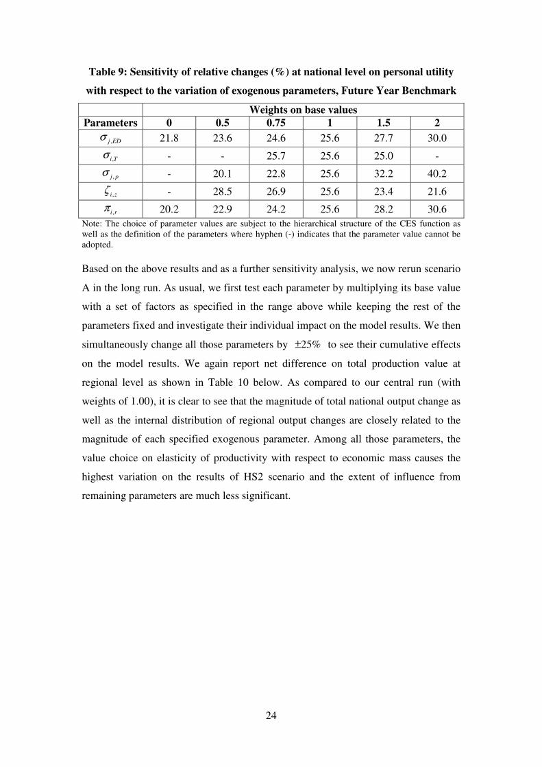
Table 9: Sensitivity of relative changes (%) at national level on personal utility

with respect to the variation of exogenous parameters, Future Year Benchmark

Weights on base values

Parameters 0 0.5 0.75 1 1.5 2

,j EDσ

21.8 23.6 24.6 25.6 27.7 30.0

,i Tσ

- - 25.7 25.6 25.0 -

,j pσ

- 20.1 22.8 25.6 32.2 40.2

,i zζ

- 28.5 26.9 25.6 23.4 21.6

,i rπ

20.2 22.9 24.2 25.6 28.2 30.6

Note: The choice of parameter values are subject to the hierarchical structure of the CES function as

well as the definition of the parameters where hyphen (-) indicates that the parameter value cannot be

adopted.

Based on the above results and as a further sensitivity analysis, we now rerun scenario

A in the long run. As usual, we first test each parameter by multiplying its base value

with a set of factors as specified in the range above while keeping the rest of the

parameters fixed and investigate their individual impact on the model results. We then

simultaneously change all those parameters by 25%± to see their cumulative effects

on the model results. We again report net difference on total production value at

regional level as shown in Table 10 below. As compared to our central run (with

weights of 1.00), it is clear to see that the magnitude of total national output change as

well as the internal distribution of regional output changes are closely related to the

magnitude of each specified exogenous parameter. Among all those parameters, the

value choice on elasticity of productivity with respect to economic mass causes the

highest variation on the results of HS2 scenario and the extent of influence from

remaining parameters are much less significant.

25

Table 10: Net differences on total production value at regional level from

respective future year benchmark, sensitivity analysis of exogenous parameters,

scenario A (HS2)

Central

Region\Weights on base values 1.00 0.00 0.50 0.75 1.50 2.00 0.75 1.25

Central London 320 187 261 296 284 -186 230 435

Inner London 373 222 311 349 331 -141 277 479

Outer London -255 -36 -115 -174 -534 -1234 -152 -379

Green Belt -280 -43 -135 -198 -533 -1068 -160 -437

Urban East -164 -26 -81 -118 -298 -550 -91 -263

Urban South East -215 -35 -106 -155 -392 -722 -118 -349

Rural East -123 -23 -65 -92 -208 -350 -66 -200

Rural South East -257 -46 -132 -188 -453 -810 -141 -413

South West -257 -69 -160 -208 -354 -420 -148 -387

East Midlands -187 -56 -125 -158 -220 -132 -110 -276

West Midlands 3854 414 1897 2805 6497 10202 2527 5610

ROUK -1304 -341 -823 -1070 -1649 -1277 -733 -2049

UK 1504 147 725 1089 2472 3313 1313 1770

Central

Region\Weights on base values 1.00 0.50 0.75 1.50 2.00 0.50 0.75 1.50 2.00

Central London 320 164 244 464 585 154 224 609 880

Inner London 373 213 295 522 649 246 311 496 547

Outer London -255 -236 -246 -267 -286 -184 -225 -294 -369

Green Belt -280 -245 -263 -310 -344 -195 -242 -336 -403

Urban East -164 -140 -152 -184 -205 -109 -139 -200 -232

Urban South East -215 -181 -199 -246 -277 -139 -181 -268 -314

Rural East -123 -104 -114 -141 -158 -93 -111 -136 -145

Rural South East -257 -216 -237 -295 -335 -180 -224 -301 -336

South West -257 -216 -237 -295 -331 -186 -228 -300 -319

East Midlands -187 -159 -174 -213 -230 -138 -166 -223 -233

West Midlands 3854 3487 3672 4202 4534 2904 3449 4450 4906

ROUK -1304 -1053 -1178 -1562 -1786 -919 -1138 -1581 -1660

UK 1504 1314 1412 1674 1816 1162 1329 1917 2321

Central

Region\Weights on base values 1.00 0.50 0.75 1.50 2.00 0.00 0.50 0.75 1.50

Central London 320 317 319 323 325 209 252 283 449

Inner London 373 371 372 375 376 244 295 331 510

Outer London -255 -274 -264 -240 -229 -133 -178 -209 -423

Green Belt -280 -297 -288 -267 -256 -136 -187 -225 -505

Urban East -164 -173 -168 -157 -151 -78 -108 -131 -306

Urban South East -215 -227 -221 -206 -198 -100 -140 -170 -408

Rural East -123 -131 -127 -117 -113 -58 -80 -98 -232

Rural South East -257 -273 -265 -245 -236 -121 -168 -205 -482

South West -257 -272 -264 -246 -237 -131 -177 -211 -435

East Midlands -187 -198 -192 -179 -173 -100 -133 -156 -306

West Midlands 3854 3952 3900 3776 3713 2172 2781 3229 6478

ROUK -1304 -1352 -1326 -1264 -1232 -641 -880 -1059 -2355

UK 1504 1443 1476 1552 1590 1129 1278 1377 1987

Central

Region\Weights on base values 1.00 0.75 1.25

Central London 320 131 918

Inner London 373 188 651

Outer London -255 -123 -627

Green Belt -280 -127 -693

Urban East -164 -73 -406

Urban South East -215 -92 -560

Rural East -123 -57 -271

Rural South East -257 -116 -620

South West -257 -133 -475

East Midlands -187 -103 -281

West Midlands 3854 1864 7630

ROUK -1304 -641 -2277

UK 1504 717 2990

*All values are measured with 2000 prices

Productivity elasticity

Transport scale

Transport elasticity

Production elasticity

All parameters

Export demand elasticity Domestic competition parameter

26

5. Conclusions

In this paper, we have demonstrated that it is feasible to develop a SCGE model at

city region level with existing data sources in the UK. The resulting model shows that

it is capable of testing a wider set of policy impacts than existing land use/transport

models and SCGE models, and the test results are often qualitatively different from

those from the existing models.

As compared with traditional land use and transport models, our model differs due to

the inclusion of Dixit-Stiglitz model of monopolistic competition among producers,

elasticity of substitution on production factors, interregional trade pooling, and the

Armington specification regarding product varieties from producers in different

locations. Relative to existing SCGE models, our extensions incorporate (1) a

specification of Hicks neutral agglomeration effects on productivity, which arise from

external increasing returns to scale induced from urbanization and transport

improvements, (2) labour mobility across the study area with both commuting and

migration, (3) counterfactual equilibrium in both short run and long run to allow for

different rates of change in the spatial distribution of economic activities and

residential location, (4) land as an explicit factor input to production, and (5) concave

transport cost functions with respect to travel distance to be consistent with realistic

transport costs.

The model results obtained are in line with theoretical expectations and provide new

quantification of the costs and benefits that feed into the assessment of those strategies.

In both transport related scenarios (A and B), the model shows how transport

improvements can lead to both shifts of production and residential population, and net

overall welfare changes. Under the business land supply increase scenario (C), the

model suggests that releasing a moderate proportion of Green Belt for development

can help boost economic growth.

To identify the sensitivity of the model results, we have carried out additional model

tests to isolate the effects of introducing agglomeration and product variety effects.

The model results indicate that it is important to incorporate both model features if

one wishes to quantify wider economic impacts. In addition to this, we have also

tested for the range of uncertainties associated with the choice of model parameter and

27

elasticity values, which provide an in-depth understanding of the results and should

inform future empirical determination of the parameter values.

In view of the findings above, we suggest following areas as possible research tasks

for the near future. First, it is preferable to replace the current iceberg representation

of transport costs with a better approach that separate the price and volume effects .

Secondly, it would be desirable to have a more detailed sectoral disaggregation for the

model's practical implementation. A straightforward disaggregation is to introduce

different types of labour by skills or socioeconomic status or a combination of them.

Thirdly, it is desirable to extend the model with a true dynamic structure for studying

intertemporal decisions of savings and investment decisions.

References

[1] Armington, P. S., A theory of demand for products distinguished by place of

production. International Monetary Staff Papers 16:159–176, 1969.

[2] Bröcker, Johannes. Operational spatial computable general equilibrium modeling.

The Annals of Regional Science, vol. 32, pp. 367-387, 1998.

[3] Bröcker, Johannes, Passenger Flows in CGE models for Transport Project

Evaluations? Paper presented to the ERSA congress 2002, Dortmund, August 2002.

[4] Bröcker, Johannes, Schneider, Martin. How does economic development in

eastern Europe affect Austria’s regions? A multiregional general equilibrium

framework. Journal of Regional Science, vol. 42, no. 2, pp. 257-285, 2002.

[5] Bröcker, J., Meyer, R., Schneekloth, N., Spiekermann, K., Wegener,M., Modelling

the spcoa-economic and spatial impacts of EU transport policy, IASON Deliverable 6,

Funded by the 5th Framework RTD programme. Kiel/Dortmund:

Christian-Albrechts-Universität Kiel/Institut für Raumplanung, Universität Dortmund,

2004.

[6] Dixit, Avinash K & Stiglitz, Joseph E, Monopolistic Competition and Optimum

Product Diversity," American Economic Review, American Economic Association,

28

vol. 67(3), pages 297-308, June, 1977.

[7] Department for Transport, Transport, Wider Economic Benefits, and Impacts on

GDP, Discussion Paper, UK, 2005.

[8] Graham, Daniel J., Agglomeration, Productivity and Transport Investment,

Journal of Transport Economics and Policy, 41, 3, 317-343, 2007.

[9] McCann, P. Transport costs and new economic geography. Journal of Economic

Geography 5, pp. 305–318, 2005.

[10] Magnani, R & Mercenier, J. On linking microsimulation and

computable general equilibrium models using exact aggregation of

heterogeneous discrete-choice making agents. Economic Modelling, Elsevier, vol.

26(3), pages 560-570, May, 2009

[11] Nijkamp, P., Rietveld, P., Snickars, F., Regional and multiregional economic

models: A survey; in: Nijkamp P. (ed.): Handbook of regional and urban economics,

Vol. 1 Regional Economics, pp. 257-294, North-Holland, Amsterdam, 1986.

[12] Samuelson, P. A., The transfer problem and transport cost, ii: analysis of effects

of trade impediments. Economic Journal 64:264–289, 1954.

[13] Schneider, Martin, Modelling the effects of the future East-West trade on

Austria’s regions. Unpublished PhD thesis, University of Viena, Vienna, 1998.

[14] Tavasszy L.A., Thissen, M., Muskens, A.C., Oosterhaven, J., Pitfalls and

solutions in the application of spatial computable general equilibrium models for

transport appraisal, paper presented at the 42nd Congress of the European Regional

Science Association, Dortmund, 2002.

[15] Thissen, M., Limtanakool, N., Hilbers, H., Road Pricing and Agglomeration

Economies - A new methodology to estimate indirect effects with an application to

the Netherlands, Paper to be presented at the 3rd Israel-Netherlands Workshop in

Regional Science, Israel, 2008.

29

Appendix A: Production sectors used in the model

The UK IO table is aggregated in the following way

Production Sector ISIC Rev.3 Code

Primary A-B

Secondary C-F

Tertiary G-Q

Appendix B: ISIC of all economic activities, Rev.3

Category Economic Activities

A Agriculture, hunting and forestry

B Fishing

C Mining and quarrying

D Manufacturing

E Electricity, gas and water supply

F Construction

G

Wholesale and retail trade; repair of motor

vehicles, motorcycles and personal and

household goods

H Hotels and restaurants

I Transport, storage and communications

J Financial intermediation

K Real estate, renting and business activities

L Public administration and defence;

compulsory social security

M Education

N Health and social work

O Other community, social and personal

service activities

P Private households with employed persons

Q Extra territorial organizations and bodies

Appendix C: List of Acronyms

ABI Annual Business Inquiry

ASHE The Annual Survey of Hours and

Earnings

NCES Nested Constant Elasticity of Substitution

HMRC Her Majesty's Revenue and Customs

ISIC International Standard Industrial

Classification of All Economic Activities

SAM Social Accounting Matrix

OECD Organisation for Economic Co-operation

and Development

VOA Valuation Office Agency

30

Appendix D: Derivation of price for the composite of zonal varieties

As mentioned in section 2.1, firms use the raw output ,i rX as the only input to

produce the variety of final output '

,i rX under monopolistic competition in the style

of Dixit-Stiglitz. For production of each variety under each sector i and zone r, it is

assumed that the firm uses a fixed amount i

χ of raw output plus a constant marginal

amount i

κ per unit of final output such that

'

, , , ,i r i r i r i rx xχ κ= + (D.1)

The firm sets its final output price '

,i rp as a constant fixed mark-up over marginal

cost ,i rp

,'

, , ,

, 1

i r

i r i r i r

i r

p pε

κε

=−

(D.2)

The output per variety is fixed in equilibrium, which takes the form of

,'

, ,

,

( 1)i r

i r i r

i r

xχ

εκ

= − (D.3)

By inserting (D.3) into (D.1), the amount of raw output used to produce each variety

is equivalent to

, , ,i r i r i rx χ ε= (D.4)

The total number of varieties ,i rn produced in each zone r is equivalent to

,

,

, ,

i r

i r

i r i r

Xn

χ ε= (D.5)

The total output of final goods '

,i rX produced in zone r can be calculated as

, , ,' '

, , , , ,

, , , , ,

1( 1)

i r i r i r

i r i r i r i r i r

i r i r i r i r i r

XX n x X

χ εε

χ ε κ ε κ

−= = − = (D.6)

If we set the unit of final output as ,

, ,

1i r

i r i r

ε

κ ε

−, we can have '

, ,i r i rX X= and '

, ,i r i rp p=

The composite of the zonal varieties has the unit cost ,i rυ in the CES form of

31

, , , ,

1 1

1 1 1 1

, , , ,

1

[ ] [ ]i r i r i r i r

N

i r i r i r i r

n

p n pε ε ε ε

υ− − − −

=

= =∑ (D.7)

By inserting (D.5) into (D.7), we can rewrite (D.7) as

, ,

1

1 1,

, ,

, ,

[ ]i r i ri r

i r i r

i r i r

Xp

ε ευ

χ ε

− −= (D.8)

In general, ,i rn (or the combination of , ,i r i r

χ ε ) is estimated based on interzonal trade

flows and it is a common practice to set both ,i rχ and ,i r

ε only sector specific but

not zonal specific. Following Tavasszy et.al (2002)[15]

, ,i rn might be better

understood as the share of zonal production in the production of all varieties within a

sector rather than being interpreted as the number of firms or varieties in a zone

because in the empirical case, it is likely that a variety is made by many firms.

Therefore, in this model, we set ,

,

,

i r

i r

i B

Xn

X= .