
Application of 3D laser scanning in monitoring of a...
14
Application of 3D laser scanning in monitoring of a barren slope Tsung-Chiang Wu, National Chung-Hsing University, Taichung, Taiwan Zheng-Yi Feng, National Chung-Hsing University, Taichung, Taiwan Wen-Fu Chen, National Chung-Hsing University, Taichung, Taiwan Abstract This study utilizes the 3D scanning technology to obtain high accuracy 3D point-cloud coordinates for a barren slope area. The data of point-clouds were scanned twice on two different dates to analyze the changes and deformations of the slope for its range, size and locations. This method can measure the 3D slope surface accurately, and improve the accuracy of comparison between the two measurements. After the proposed post-process procedures, this study shows that 3D laser scanning technology is very useful in monitoring barren slope for its movement, changes, sliding volume, etc. Further applications for slope/landslides should include understanding long-term creep tendency, detection of the extent of landslide and prediction/warning of future sliding. 1. Introduction Under Taiwan’ s special climate conditions, intense rainfalls always trigger landslides during long typhoon season in summer. When there are residents/facilities close to the landslide areas, actions are often taken to reduce the risks due to the landslides. More often than not there could be no long enough timeslot for us to perform mitigation work immediately, the landslide area may keep enlarging and continue to deform. In order to better understand the activity of a landslide, monitoring approaches are often suggested. However, traditional landslide monitoring uses surveying, physical measurement equipments (such as inclinemeter) and/or accurate measurement method (such as accurate Global Positioning System, GPS) to detect activities of landslides. The monitoring work is always time consuming and the data are not enough for a comprehensive terrain changing analysis. Further, if the landslide area is inaccessible (or of dangerous), only a very limited topographical data can be obtained. Mitigation decision of the landslide will be delayed or affected. Therefore, this study is aiming at developing a continuous monitoring and analyzing
Transcript of Application of 3D laser scanning in monitoring of a...

Application of 3D laser scanning in monitoring of a barrenslope
Tsung-Chiang Wu, National Chung-Hsing University, Taichung, Taiwan
Zheng-Yi Feng, National Chung-Hsing University, Taichung, Taiwan
Wen-Fu Chen, National Chung-Hsing University, Taichung, Taiwan
AbstractThis study utilizes the 3D scanning technology to obtain high accuracy 3Dpoint-cloud coordinates for a barren slope area. The data of point-clouds werescanned twice on two different dates to analyze the changes and deformationsof the slope for its range, size and locations. This method can measure the 3Dslope surface accurately, and improve the accuracy of comparison betweenthe two measurements. After the proposed post-process procedures, thisstudy shows that 3D laser scanning technology is very useful in monitoringbarren slope for its movement, changes, sliding volume, etc. Furtherapplications for slope/landslides should include understanding long-term creeptendency, detection of the extent of landslide and prediction/warning of futuresliding.
1. Introduction
UnderTaiwan’s special climate conditions, intense rainfalls always trigger landslides during
long typhoon season in summer. When there are residents/facilities close to the landslide
areas, actions are often taken to reduce the risks due to the landslides. More often than not
there could be no long enough timeslot for us to perform mitigation work immediately, the
landslide area may keep enlarging and continue to deform. In order to better understand the
activity of a landslide, monitoring approaches are often suggested. However, traditional
landslide monitoring uses surveying, physical measurement equipments (such as inclinemeter)
and/or accurate measurement method (such as accurate Global Positioning System, GPS) to
detect activities of landslides. The monitoring work is always time consuming and the data are
not enough for a comprehensive terrain changing analysis. Further, if the landslide area is
inaccessible (or of dangerous), only a very limited topographical data can be obtained.
Mitigation decision of the landslide will be delayed or affected.
Therefore, this study is aiming at developing a continuous monitoring and analyzing

approaches for barren slope/landslide areas using advanced 3D laser scanning
(ground-based Light Detection And Ranging, LiDAR). The 3D laser scanner was utilized to
obtain a large amount of accurate 3D coordinates of a slope for representing its terrain
topography. Also, the technique was applied for analyzing of the terrain changes and
deformation of the sliding area, including calculation of the volumes of accumulation and
depletion zones that occurred during a 45-day period. Recommendations are also given for
handling of possible error sources during data interpretations.
2. Research methodology
A slope after mining near Mountain Pillow in Taiwan was selected for the study (Fig. 1). The
3D scanner was used to measure the first point-cloud data set of the slope surface. After 45
days, the scanner was used again to obtain the second data set. The two sets of data were
analyzed for slopes changes. The two sets of data were compared by matching the
coordinates of the fixed“conjugate scanning spheres”(Fig. 3) and transforming the
coordinate systems of different scanning stations. The method and principle are described
as following.
Fig. 1 A slope after mining near Mountain Pillow in Taiwan
2.1 3D laser scanning technology and processing method
“Time of flight”scanning principle of 3D laser scanner is used to calculate the distance () in
EQ.2.1 between the scanner and the object (Fig. 2) using speed of light (c) and the travel time
(△t). Impulse laser light is produced form the diode of the scanner and the signal reflected
back from the surface of the object will be received.
tc21 ………………………………………EQ.2.1

Fig. 2 Time of flight(Boehler, 2001)
We need to first set up the 3D laser scanner in a proper scanning station nearby the landslide
slope. The scanning station is required to be set within the effective scanning distance of the
scanner. For this case, it is 200 meters between the scanner and the objects to be scanned. At
least three conjugate scanning spheres should be installed for matching process.
Fig.3 Scanning station and the 3D scanner (left) and one of the conjugate scanning spheres
(right).
2.2 Coordinate system transformation of different scanning stations
The two scanning operations used two different scanning stations. When overlapping the two
scanned data sets, we choose the first scanning station to be the“base”coordinate system,
and the coordinate system of second scanning station is transformed to the base coordinate
system. The conjugate scanning spheres will be the common (matching) points of the two sets
of scanned data. Fig. 4 shows the spatial coordinate relationship between the scanning
stations and a conjugate scanning sphere. S is the position of the second laser scanner. P is
the position of a conjugate scanning sphere. O is the position of the“base”laser scanner (base

coordinate system). is the distance from S to P. αis the plunge angle of SP referring to
the xy-plane of the second coordinate system,and θis the angle between the projection line of
SP on the xy-plane and x-axis of the second coordinate system.
Fig. 4 The spatial coordinate relationship between scanning stations and conjugate
scanning spheres(modified from Lichti, 2002)
The mathematic formula of the coordinate system of second scanning station transformed to
the base coordinate system is shown as in EQ.2.2. The coordinates of the three or more
conjugate scanning spheres are used for coordinate matching and transformation.
p p sR M r R
……………………………EQ.2.2
where,T
p p p pr x y z
: the vector coordinate of conjugate spheres in base
coordinate system;
T
p p p pR X Y Z
: the vector coordinate of conjugate spheres in the second
coordinate system;
Ts s s sR X Y Z
: the vector coordinate of the second coordinate system after
transformed into the base coordinate system;
M is the rotation matrix of X-, Y-, Z-axis and the angles (, , ).

cos cos cos sin sin cos sin sin cos sin coscos sin cos cos sin sin sin cos cos sin sin
sin sin cos cos cos
sinM sin
2-3 The approach of overlapping analysis for terrain changes and deformation
The purpose of overlapping analysis of the two sets of 3D point-cloud data is to calculate for
terrain changes and deformation. After the second set of the data has been transformed to the
base coordinate system using the method introduced in previous section, the difference of the
surface changes/variations between the two sets of data can be calculated using the
procedures proposed below.
(a) Using Triangulated Irregular Network (TIN) to build a surface from a set of irregularly
spaced points for each set of the two scanned point-cloud data (Fig. 5).
Fig. 5 The 3D point-cloud data (left); the surface model composed using TIN (right).
(b) Importing the two TIN surface models to a same coordinate system, then calculate the
vertical difference distances between the two TIN surfaces. It is done by finding the
coordinates of all the vertices of the triangles of first TIN surface, then extending vertical lines
in Z-axis direction from the vertices to intercept the second TIN surface as shown in Fig.6, and
locating the coordinates of the interception points. 6; finally, calculating the vertical difference
distance ( nZ ) between the vertex and the interception point. We consider that a nZ value
is the variation amount at a single point of the first scanning.
In a TIN surface model, the planar equation for a triangle is:
0DCZBYAX .
The three vertices of a triangle are: I ),,( 111 ZYX 、J ),,( 222 ZYX 、K ),,( 333 ZYX . Therefore,

)()()(
12
31
32
3
2
1
ZZZZZZ
YYY
A
T
,
)()()(
12
31
32
3
2
1
XXXXXX
ZZZ
B
T
,
)()()(
12
31
32
3
2
1
YYYYYY
XXX
C
T
, and
111 CZBYAXD .
On any triangle,CD
YCB
XCA
Z ……………………………EQ.2.3
Assume that ),,( 111 cbaP and ),,( 222 cbaQ are two points in space, then the line equation
passing through Point P and Q in space is:
RttcccZtbbbYtaaaX
L ,)()()(
:
121
121
121
.
If the line L parallel to Z-axis, then 2121 , bbaa ; therefore,
RttcccZ
bYaX
L ,)(
:
121
1
1
.
Assume ),,( ddd ZYXD is a point on the spatial line L, then the distance from Point D to the
interception point ),,( eee ZYXE is:
CD
YCB
XCA
ZZZS ddede , ……………………EQ.2.4
The S in EQ.2.4 is the difference between the two TIN surface models (Fig.6). If 0 de ZZ ,
the ground surface is accumulating. If 0 de ZZ , ground surface is no change. If
0 de ZZ , the ground surface is depleting.

Fig. 6 Vertical difference distances between the two TIN surfaces (referring to the 1st
scanned face)
2.4 Flowchart of the approaches (Fig. 7)
The approaches of handling the scanned data for the study introduced in Section 2 are
summarized in Fig. 7. The data processing results of the approaches are shown in Section 3.
Perform two scanning for a slope/landslide on different dates. Obtain 3D point-cloud data.
Transform the second scanned data to the first scanning base coordinate system.
Check the positions of conjugate scanning spheres. If it is moved, delete the point. If it is not
disturbed, keep the points to be the matching points while coordinate transformation.
Build TIN surface models for the two scanned data, and import the two models to a same
coordinate system for overlapping analysis.
Calculate differences between the two surface models for terrain variations. Verify the variation
results.
Fig.7 Flowchart of the approaches
I
JK
Vertical spatial line
S
The 2nd scanned face
The 1st scanned faceD
E

3. Data processing
3.1 Perform two scanning for a slope/landslide on different dates. Obtain 3D point-cloud data.
The 3D point-cloud data from the two scanning operations are shown in Fig. 8.
Fig. 8 3D point-cloud data from the first scanning (left) and the second scanning (right)
Table1 Distances back-calculated between conjugate scanning spheres for the two scanning
operations (unit: mm)
Distance
(conjugate
sphere to
conjugate
sphere)
Distance
back-calculated
from the first
scanning
coordinate
Distance
back-calculated
from the second
scanning
coordinate
Distance
error
Distance
error/distance,
(accuracy)
d01-d02 6090.07 6084.71 -5.36 1/1135.68, (1135.68)
d01-d03 3247.27 3241.61 -5.66 1/573.91, (573.91)
d01-d04 5267.73 5255.42 -12.31 1/427.88,(427.88)
d02-d03 7060.47 7059.42 -1.06 1/6674.47,(6674.47)
d02-d04 3184.85 3183.72 -1.13 1/2820.60,(2820.60)
d03-d04 4698.10 4693.85 -4.25 1/1104.59,( 1104.59)
3.2 Check the positions of conjugate scanning spheres. If it is moved, delete the point. If it is
not disturbed, keep the points to be the matching points while coordinate transformation.
The distances back-calculated between conjugate scanning spheres (d01, d02, d03, d04) for
the two scanning operations are listed in Table 1. As shown in Table 1, the distance accuracy
of d01-d03 and d01-d04 are smaller than 1000; the others are all larger than 1000. It means
that the conjugate sphere d01 may had been tempered during the two scanning operations.

Therefore, we should delete d01 from being matching point, and use d02, d03, d04 as the
common points for further matching calculations.
3.3 Transform the second scanned data to the first scanned base coordinate system.
Table 2 presents the results of transforming the second scanning coordinate of conjugate
scanning sphere to the base coordinate system. It also shows that the maximum error is
7.34mm, and the minimum error is -0.01mm.
Table2 Coordinates of the conjugate scanning spheres transformed to the base coordinate
system (unit: mm)
Conjugate
sphere
First scanning (base) coordinate
system(E1)
Second scanning coordinate system
(E2)
X Y Z X Y Z
d02 3180.93 -11304.39 -1738.54 -13286.04 113.27 -1842.69
d03 7770.54 -16652.16 -2171.14 -19880.49 -2364.72 -2299.04
d04 3626.09 -14451.34 -1942.97 -16393.86 768.82 -2061.49
Conjugate
sphere
E2 transformed to E1 Error of transform
X Y Z X Y Z
d02 3183.03 -11304.27 -1738.62 2.10 0.12 -0.08
d03 7772.93 -16650.40 -2171.15 2.39 1.76 -0.01
d04 3633.43 -14449.33 -1943.07 7.34 2.01 -0.10
3.4 Build TIN surface models for the two scanned data, and import the two models to a same
coordinate system for overlapping analysis.
The two sets of point-cloud data were used to build TIN surface models as shown in Fig. 9 and
Fig.10. Overlapping of the two sets of point-cloud data and TIN models are shown in Fig.11.

Fig. 9 The first scanning point-cloud data (left) and TIN model (right)
Fig. 10 The second scanning point-cloud data (left) and TIN model (right)
Fig. 11 Overlapping of the two sets of point-cloud data (left) and TIN models (right).

3.5 Calculate differences between the two surface models for terrain variations.
Enlarged TIN models are shown in Fig. 12. The difference (surface changes) between the two
scanning surfaces can be calculated using the method introduced in Section 2.3. The
differences of each vertex can be used for interpolation in TIN model to show the surface
variations using various colors as shown in Fig.13.
Fig. 12 Overlapping TIN model for a flat zone (upper left); vertices of triangles of the first
scanning TIN surface for a flat zone (upper right); Overlapping TIN model for a undulate zone
(lower left); vertices of triangles of the first scanning TIN surface for a undulate zone (lower
right). Note: The first scanning TIN is shown in red color, and the second scanning TIN in grey.
Fig. 13 Surface variations of a flat zone (left); Surface variations of a undulate zone shown by
various colors (right).

4. Result discussions
The surface variation result after data processing is shown in Fig. 14. The dark blue color is
where no variation occurs. They are evenly distributed and consisting with in-situ condition.
The non- dark blue parts are the variation zones. It also fits the in-situ changes very well. While
scanning, some surfaces may be blocked due to terrain, obstacles and scanning angle.
Therefore, no point-cloud data for those surfaces can be obtained. For example, the red
rectangle area in Fig. 14 (also refer to Fig. 8). During data processing, the no-data areas have
to be assumed values by interpolation.
The variations shown in the black rectangle areas in Fig. 14 are due to weeds growing on the
slope surface during the two scanning dates. To prevent misjudgment on surface variation,
the changes and deformation should be verified with site photos as shown in Fig. 15.
There are some green color (and some red color) areas in Fig. 14. The areas are mostly
surface cracks or larger undulate areas and they are not surface variation. This could be due
to the two scanning stations were not set at a same location. Some discrepancies in
interpolation for blocked surface could be generated. Therefore, we suggest installation of a
fixed base-plate for scanning station to maintain a same scanning location.
For the red color areas in Fig. 14, it is where the variations are greater than 40cm. It can be a
local sliding. The yellow rectangle area as shown in Fig. 14 is the sliding area identified by this
study and can be compared to the site photo as shown in Fig.16.
Fig. 14 The surface variation result after overlapping the two scanned data sets.
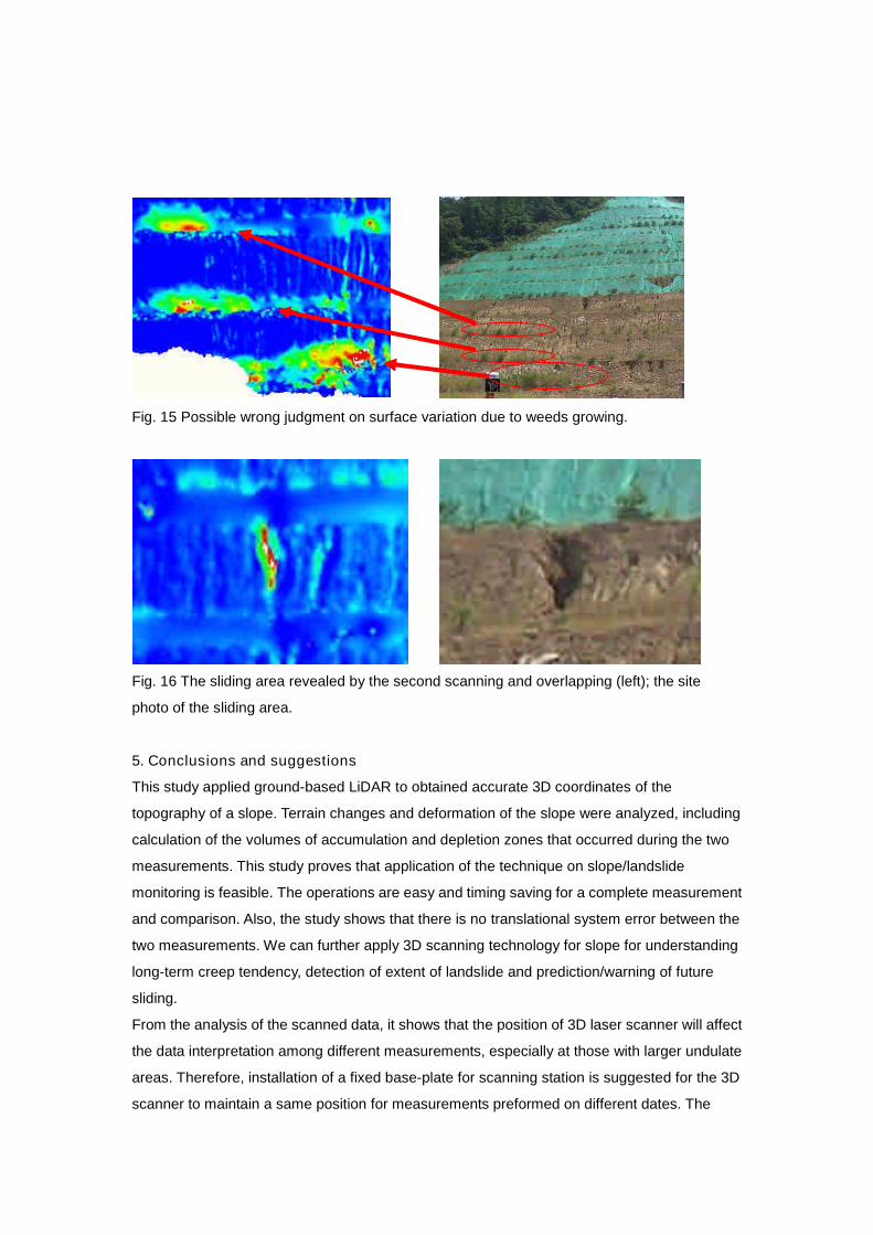
Fig. 15 Possible wrong judgment on surface variation due to weeds growing.
Fig. 16 The sliding area revealed by the second scanning and overlapping (left); the site
photo of the sliding area.
5. Conclusions and suggestions
This study applied ground-based LiDAR to obtained accurate 3D coordinates of the
topography of a slope. Terrain changes and deformation of the slope were analyzed, including
calculation of the volumes of accumulation and depletion zones that occurred during the two
measurements. This study proves that application of the technique on slope/landslide
monitoring is feasible. The operations are easy and timing saving for a complete measurement
and comparison. Also, the study shows that there is no translational system error between the
two measurements. We can further apply 3D scanning technology for slope for understanding
long-term creep tendency, detection of extent of landslide and prediction/warning of future
sliding.
From the analysis of the scanned data, it shows that the position of 3D laser scanner will affect
the data interpretation among different measurements, especially at those with larger undulate
areas. Therefore, installation of a fixed base-plate for scanning station is suggested for the 3D
scanner to maintain a same position for measurements preformed on different dates. The

analysis results of this study can indicate the position of changes and deformations of a slope.
However, the changes and deformation should be verified with site photos to avoid making
wrong judgment.
6. References[1] Boehler, W., G.Heinz, A. Marbs, 2001. The Potential of Non-contact Close Range Laser
Scanners for Cultural Heritage Recording, Proceedings of CIPA International Symposium,Potsdam, Germany.
[2] Gordon, Stuart, Derek Lichti and Mike Stewart, 2001. Application of a High-ResolutionGround-baesd Laser Scanner for Deformation Measurements, 19–22 March 2001Orange, California, USA 23
[3] Zheng-yi Feng, Jia-Chi Liang, Tzong-Jiang Wu 2006.Three-dimensional LaserScanning and Stability Analysis of Slopes, Journal of Soil and Water Conservation, Vol.38,No.2, pp.117-128 (in Chinese).