Application LGD Model Development - CRC · available. However, if such accounts are excluded from...

© Experian Limited 2009. All rights reserved. Experian and the marks used herein are service marks or registered trademarks of Experian Limited.Other product and company names mentioned herein may be the trademarks of their respective owners. No part of this copyrighted workmay be reproduced, modified, or distributed in any form or manner without the prior written permission of Experian Limited.

Application LGD Model Development

A Case Study for a Leading CEE BankStefan Stoyanov, Solutions Manager, Experian Decision Analytics

Credit Scoring and Credit Control XI Conference

Edinburgh, 26th-28th of August 2009

© Experian Limited 2009. All rights reserved. 2

Introduction

The presentation discusses three alternative LGD application scorecarddevelopment methodologies applied to a Private Individuals Car Leasingportfolio of a leading bank operating in Central and Eastern Europe

The presentation is divided in two sections:

The first section is focused on the sampling methodology, LGDcalculations and treatment of censored observations (incompleteworkouts)

The second part of the presentation describes the LGD modelling andvalidation methodologies

The presentation concludes with a comparison between the three alternativeLGD models discussing the pros and cons of each approach, including arecommendation for the final model selection


Advantages of developing an application LGD model

The combination of PD and LGD scorecards helps banks optimise theirdecision making process with regards to lending

With the traditional scoring systems, the clients are graded based on theirprobability of default. A LGD application scorecard allows the estimation of thesecond parameter that characterises loan risk - the loss given default or LGDat origination stage

Hence, the LGD scoring model can add a new dimension to the risk rating, byclassifying the clients in terms of the expected final loss rate in case of default

For example, for two applicants with the same PD but different LGDs the finaldecision should therefore be based on the Expected Loss Rate:

ELR=PD*LGD

Hence, a better assessment of the credit risk at the time of application can beachieved by combining two statistical models (PD and LGD)


Agenda

Development Sample Selection

LGD Calculation

LGD Transformations

Calibration of the Logistic Regression Scores to Estimated LGD

LGD Model Validation Tests

LGD Models Comparison


Default window for LGD application model developmentMethodological approach

For sample definition 12 months of fixed default observation period fromapplication date were used in order to link the PD and LGD model estimatessince they will be combined in the capital calculation

Risk-Based Capital Standards: US Advanced Capital Adequacy Framework—Basel II; Final Rule (December 2007)Par. Economic Loss and Post-Default Extensions of Credit“LGD is an estimate of the economic loss that would be incurred on an exposure,relative to the exposure’s EAD, if the obligor were to default within a one-year horizonduring economic downturn conditions”

Risk-Based Capital Standards: US Advanced Capital Adequacy Framework—Basel II; Final Rule (December 2007)Par. Economic Loss and Post-Default Extensions of Credit“LGD is an estimate of the economic loss that would be incurred on an exposure,relative to the exposure’s EAD, if the obligor were to default within a one-year horizonduring economic downturn conditions”


Development sampleDefinitions and selection criteria

It is the period during which the defaults are observed

A fixed 12 months observation period was used for thisdevelopment (12 months from application date)

Only the defaults which occurred during this period were includedin the model development sample

Defaultobservation

period

Defaultobservation

period

Outcomeperiod

Outcomeperiod

It is the period during which the LGD is observed (LGD outcomeperiod)

A maximum of 12 months of outcome period were useddepending on whether the account was cured, closed or still incollections


2° defaultdate

2° defaultdate

Development sampleAccounts with multiple defaults

If an account defaulted more than once during the default observation periodonly the last default event was included in the development sample

Consequently, the LGD was measured at such event (EAD, costs andrecoveries related to it)

Accountcured

Accountcured

1° defaultdate

1° defaultdate

Jan05 Jan07

Default observation period

Feb08Feb06

ApplicationDate

ApplicationDate

Jul06 Dec06Sep06

LGD outcome period

Only the last default event was included in themodel development sample


Agenda


LGD Calculation

LGD Transformations





LGD components – car leasing portfolio

Exposure atdefault (EAD)

Exposure at Default = Outstanding balanceat time of default, corresponding to:

Principal Amount + Arrears Amount

Cash recoveries

Non-cash recoveries (repossession value)Recoveries

Internal andexternal

collection costs

Internal costs = direct and indirect costs

External collection costs = costs forexternal collection agencies

Annual Percentage Rate wasused as a discount factor in thecalculation of the net presentvalues of the recoveries andcosts


LGD calculationDefault categories

Default observation window: first 12months from application date

LGD outcome period: Censoring point at 12 months outcome history

Defaultedaccounts

Not cured

2. Closed2. Closed

3. Open (Incompleteworkouts)

3. Open (Incompleteworkouts)

Cured 1. Closed / Open1. Closed / Open

Final loss available

Final loss not available

Order of default selection

Three categories of defaulted accounts were selected based on the criteria forLGD calculation :


LGD calculationModelling approach in case of incomplete recovery history

For the open not cured accounts only incomplete recovery history isavailable. However, if such accounts are excluded from the modeldevelopment sample it would introduce bias in the LGD estimates

The firms can consider the incomplete workouts in their LGD estimates butestimations about future costs and recoveries are not allowed (BKI – Supervisoryregulations. Title II – Chapter 1 Par. 2.3)

It would be wrong to ignore the incomplete workouts in the LGD estimates(FSA Staff Paper: Own estimates of Loss Given Default (Nov 2005) - Cures and Incomplete Workouts)

Modelling approach

Considering the high level of sophistication and complexity of the models that could be used to estimate the finalLGD for incomplete workouts compared to the provided benefits in terms of estimation accuracy, it was decidedto use a censoring point at 12 months for such accounts without attempting to forecast their final LGD usingstatistical models

Modelling approach

Considering the high level of sophistication and complexity of the models that could be used to estimate the finalLGD for incomplete workouts compared to the provided benefits in terms of estimation accuracy, it was decidedto use a censoring point at 12 months for such accounts without attempting to forecast their final LGD usingstatistical models


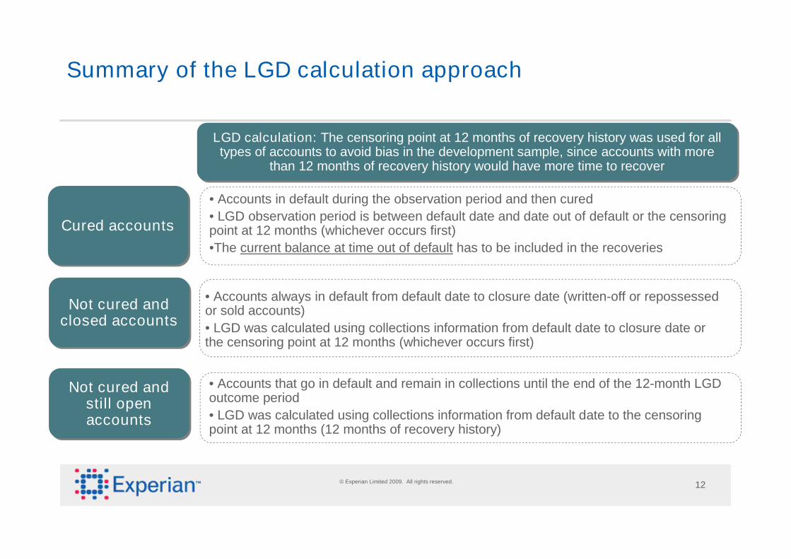
LGD calculation: The censoring point at 12 months of recovery history was used for alltypes of accounts to avoid bias in the development sample, since accounts with more

than 12 months of recovery history would have more time to recover

LGD calculation: The censoring point at 12 months of recovery history was used for alltypes of accounts to avoid bias in the development sample, since accounts with more

than 12 months of recovery history would have more time to recover

Summary of the LGD calculation approach

• Accounts in default during the observation period and then cured

• LGD observation period is between default date and date out of default or the censoringpoint at 12 months (whichever occurs first)

•The current balance at time out of default has to be included in the recoveries

Cured accountsCured accounts

• Accounts always in default from default date to closure date (written-off or repossessedor sold accounts)

• LGD was calculated using collections information from default date to closure date orthe censoring point at 12 months (whichever occurs first)

• Accounts that go in default and remain in collections until the end of the 12-month LGDoutcome period

• LGD was calculated using collections information from default date to the censoringpoint at 12 months (12 months of recovery history)

Not cured andclosed accountsNot cured and

closed accounts

Not cured andstill openaccounts

Not cured andstill openaccounts


Agenda


LGD Calculation

LGD Transformations





LGD transformations

Both linear and logistic regression models were built in order to determine which of them provides the bestestimate of the observed LGD.

Linear regression - continuous dependent variable

In order to meet the statistical requirements of the OLS regression an attempt was made to transform the LGD tonormality or at least symmetry by using Box – Cox type of transformation function

Logistic regression – the LGD was transformed to a binary dependent variable using two methods:

Uniform random number: if LGD > random number then LGD Binary = 1 (Bads) ; else LGD Binary = 0 (Goods)

Manual Cut-Off: if LGD > 0.2 then LGD Binary = 1 (Bads) ; else LGD Binary = 0 (Goods)

00.2727143170.243758

0.024264

0.024092

LGD

10.007115099

00.888345209

LGD BinaryRN

10.20.243758

0.024264

0.024092

LGD

00.2

00.2

LGD BinaryManual Cut-Off

An example of using uniform random numbers for assigning binary outcome

An example of using manual cut-off for assigning binary outcome


Power transformation of the LGD distribution

A Box-Cox type of transformation towardsnormality could not improve the symmetry of thedistribution of the LGD, as there were large spikesat 0 and 100 while the middle range of thedistribution was almost flat

0

100

200

300

400

500

600

0.00

001

0.04

5464

091

0.09

0918

182

0.13

6372

273

0.18

1826

364

0.22

7280

455

0.27

2734

545

0.31

8188

636

0.36

3642

727

0.40

9096

818

0.45

4550

909

0.50

0005

0.54

5459

091

0.59

0913

182

0.63

6367

273

0.68

1821

364

0.72

7275

455

0.77

2729

545

0.81

8183

636

0.86

3637

727

0.90

9091

818

0.95

4545

909

Mor

e

Bin

Fre

qu

en

cy

0.00%

10.00%

20.00%

30.00%

40.00%

50.00%

60.00%

70.00%

80.00%

90.00%

100.00%

Frequency Cumulative %

Usually the LGD has highly non-normaldistribution, often with an U shape andspikes at the two tails of the distribution

However, the basic properties of theleast squares regression do not requirenormality

Non-normality does not affect theestimation of the regression parameters.The least squares estimates are stillBLUE (best linear unbiased estimates) ifthe other regression assumptions are met

Non-normality affects the tests ofsignificance and the confidence intervalestimates of the regression parameters


Binary transformation of the LGD using uniform randomnumbers

As expected, the majority of the records where the LGD was transformed toBinary =1(Bads) were at the higher end of the LGD distribution

The random number procedure resulted in a sufficient number of Bads in thedevelopment sample in order to build robust statistical model using logisticregression Capped LGD vs Binary LGD

-0 .1

0

0 .1

0 .2

0 .3

0 .4

0 .5

0 .6

0 .7

0 .8

0 .9

1

0 200 400 600 800 1000 1200 1400 1600 1800 2000

B ina ry LG D w ith R andom N um ber Trans fo rm a tion C apped LG D


Binary transformation of the LGD using uniform randomnumbers - Simulations(1/4)

Simulations Step 1: Fit actual LGD distribution to theoretical Beta distribution

Goodness of fit:

Actual LGD is plotted against the theoretical Betadistribution

R2 = 0.99469

Theoretical Beta distributionparameters:

The estimation of the alpha (a) and beta(b) parameters of the theoretical betadistribution was based on the first twomoments of the observed LGDdistribution:

a = 0.070

b = 0.147

Original v. Beta distribution LGD

y = 0.99469x - 0.00179

R2 = 0.99469

0

0.2

0.4

0.6

0.8

1

1.2

0 0.2 0.4 0.6 0.8 1 1.2

Beta LGD

Ori

gin

al

LG

D

Generated Linear (Generated)



Simulations Step 2: Test the binary transformation bias

Estimate and test the binary transformation bias:

Generate large number of samples with beta distributions. The samplesare with size equal to the development sample size. The betadistributions have the parameters estimated in the previous step

For each sample transform the theoretical LGD to binary variable usinguniform random numbers

For each sample calculate the transformation bias as:

Bi = Mean (Beta ) / P(Binary = 1) – 1

Calculate the mean value Mean (B) and the variance Var (B) for thetransformation bias across all samples

Test the H0 (B=0) against H1(B<>0) with a t-test



For the total model development sample the t-test results indicated that thenull hypothesis that the average transformation bias is zero could not berejected at the usual confidence levels

t-test results: t-value -0.40, p-value 0.6861

Based on the evidence from the simulation results itcould be concluded that the average transformationbias for the total development sample caused by thetransformation of the actual LGD to binary variableusing uniform random numbers was negligibly small.



Simulations were also used to investigate the average transformation bias perLGD band

The t-tests results indicated that for the majority of the LGD bands the nullhypothesis that the average transformation bias is zero could not be rejected atthe usual confidence levels

Based on the evidence from thesimulation results it could be concludedthat for the majority of the LGD bandsthe average transformation bias causedby the transformation of the actual LGDto binary variable using uniform randomnumbers was negligibly small.

LGD Scoreband LGD Range t-value p-value t-test results1 0- 0.0199 11.89 0 reject Ho2 0.02-0.069 1.92 0.055 can not reject Ho3 0.07-0.119 -1.19 0.237 can not reject Ho4 0.120-0.269 1.16 0.249 can not reject Ho5 0.270-0.319 -0.19 0.849 can not reject Ho6 0.320-0.369 -0.41 0.679 can not reject Ho7 0.370-0.419 0.17 0.864 can not reject Ho8 0.420-0.769 -0.29 0.768 can not reject Ho9 0.770-0.819 -1.52 0.128 can not reject Ho

10 0.820-0.869 -0.65 0.518 can not reject Ho11 0.870-0.919 0.7 0.482 can not reject Ho12 0.920-High 1.04 0.298 can not reject Ho


Binary transformation of the LGD using manual cut-off

The manual cut-off which was used was 20% LGD. Hence, if LGD > 0.2 thenLGD Binary = 1 (Bads) ; else LGD Binary = 0 (Goods)

The transformation of the LGD to binary variable using manual cut-off resulted ina higher number of Bads compared to the uniform random numbers procedure

After the manual cut-off transformation the average LGD in the modeldevelopment sample was 36.90% which was higher than the observed averageLGD of 32.37%

After the uniform random numbers transformation the average LGD in the modeldevelopment sample was 32.93% which was very close to the observed averageLGD of 32.37%


Agenda


LGD Calculation

LGD Transformations





Functional calibration of the logistic regression scoresto estimated LGD

The OLS regression model provides direct LGD estimates whereas thelogistic regression models provide indirect LGD estimates. Hence, it isnecessary to calibrate the logistic regression scores to direct LGD estimates inorder to be able to compare the two types of models

After obtaining the functional relationship between the logistic regressionscores and LGD it is possible to assign an estimated LGD to each individualscore

Calibration of Binary Logistic Regression Score to LGD

Estimates

y = -0.0000001x4 - 0.0000500x3 - 0.0046242x2 + 0.1733534x + 52.3435880

R2 = 0.9835234

0

10

20

30

40

50

60

-250 -200 -150 -100 -50 0 50

Average Score

Absolute average calibration bias: 0.11%


Agenda


LGD Calculation

LGD Transformations





LGD model validation tests

Due to the small sample size all data were used for model development. Themodels were validated using bootstrap techniques

The following calibration tests were used to validate the LGD models:

–Spearman’s Rank Correlation

–Mean Squared Error

–R-square

–Wilcoxon Signed-Rank Test

–Continuous Gini

The results from the 5 statistical tests indicated similar performance of thelogistic and linear LGD regression models in terms of LGD estimation accuracy

The bootstrap validation results also indicated stable performance of thelinear and logistic regression models


Agenda


LGD Calculation

LGD Transformations





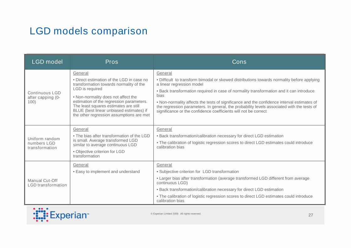
LGD models comparison

General

• Easy to implement and understand

General

• The bias after transformation of the LGDis small. Average transformed LGDsimilar to average continuous LGD

• Objective criterion for LGDtransformation

General

• Direct estimation of the LGD in case notransformation towards normality of theLGD is required

• Non-normality does not affect theestimation of the regression parameters.The least squares estimates are stillBLUE (best linear unbiased estimates) ifthe other regression assumptions are met

Pros

General

• Subjective criterion for LGD transformation

• Larger bias after transformation (average transformed LGD different from averagecontinuous LGD)

• Back transformation/calibration necessary for direct LGD estimation

• The calibration of logistic regression scores to direct LGD estimates could introducecalibration bias

General

• Back transformation/calibration necessary for direct LGD estimation

• The calibration of logistic regression scores to direct LGD estimates could introducecalibration bias

General

• Difficult to transform bimodal or skewed distributions towards normality before applyinga linear regression model

• Back transformation required in case of normality transformation and it can introducebias

• Non-normality affects the tests of significance and the confidence interval estimates ofthe regression parameters. In general, the probability levels associated with the tests ofsignificance or the confidence coefficients will not be correct

Cons

Uniform randomnumbers LGDtransformation

LGD model

Manual Cut-OffLGD transformation

Continuous LGDafter capping (0-100)


Summary

The three scorecards included the same set of risk drivers of LGD. Thesimilarity of the risk drivers indicated that little information was lost during thetransformation of the LGD to binary variable

EDA recommended the stepwise logistic regression model with uniformrandom numbers transformation of LGD to binary variable for the followingreasons:

The bias introduced by the uniform random numbers transformation was negligiblecompared to the bias introduced by the manual cut-off transformation

The logistic regression model with uniform random numbers transformation had morecharacteristics and hence better granularity of the score especially when compared to thelinear regression model

The logistic regression model was more robust compared to the linear regression model asthe shape of the LGD distribution did not affect the statistical properties of the modelparameters


Questions and Answers

&

© Experian Limited 2009. All rights reserved. Experian and the marks used herein are service marks or registered trademarks of Experian Limited.Other product and company names mentioned herein may be the trademarks of their respective owners. No part of this copyrighted workmay be reproduced, modified, or distributed in any form or manner without the prior written permission of Experian Limited.

Application LGD Model Development

A Case Study for a Leading CEE Bank

Application LGD Model Development - CRC · available. However, if such accounts are excluded from...

Documents

Transcript of Application LGD Model Development - CRC · available. However, if such accounts are excluded from...