Copyright 2013, Pipeline Simulation Interes t Group This paper was prepared for presentati on at the PSIG Annual Meeti ng held in Prague, Czech Republic, 16 April – 19 April 2013. This paper was selected for presentation by the PSIG Board of Directors followi ng revi ew of information contai ned in an abs tract submitted by the author(s). The material, as presented, does not necess arily reflect any positi on of the Pipeline Si mulation Interes t Group, its officers, or members. Papers presented at PSIG meetings are subject to publica tion review by Editorial Committees of the Pi peline Simulation Interest Group. Electr onic reproducti on, distribution, or storage of any part of this paper for commercial pur poses without the written consent of PSIG is prohibited. Permissi on to reproduce in print is restricted to an abstract of not more than 300 words ; illustrations may not be copied. The abs tract mus t contai n conspicuous acknowledgment of where and by whom the paper was presented. Write Li brarian, Pipeline Simulation Interest Group, P.O. Box 22625, Houst on, TX 77227, U.S.A., fax 01-713-586-5955.

Abstract This paper addresses the main benefit of the new integrated Pipeline Management System (PMS) for Gassco’s subsea pipeline network. The online simulation software is applied to the subsea single phase pipeline network of 7,800 km (4,847 mile) length. With the successful implementation of the simulation software integrated with the SCADA system, Gassco control room operators are able to run the complex networks confidently, reliably and predictively. A few real life operating scenarios will be used to demonstrate the commercial and technical benefits of the online software:

• Blending quality peaks passing a subsea mixing point using peak tracking

• Blending peaks after pressure levelling two pipelines using look-ahead (LAH) simulations

• Increased capacity utilisation using look-ahead predictive simulations

• Increased short term sales using look-ahead predictive simulations

• Notification of off-specification deliveries

A comparison of some of the characteristics and typical settings of the new PMS and the previous system are presented to add understanding of how these benefits arise. To illustrate how the required accuracy of the PMS can be achieved without any subsea measurements, key aspects of the tuning mechanisms will be investigated:

• Network Model Calibration through the tuning of heat transfer to improve accuracy of calculated inventory and secure accurate ETA’s.

• The use of the Maximum Likelihood State Estimation.

• Tuning of flow meter offsets and pipeline efficiency.

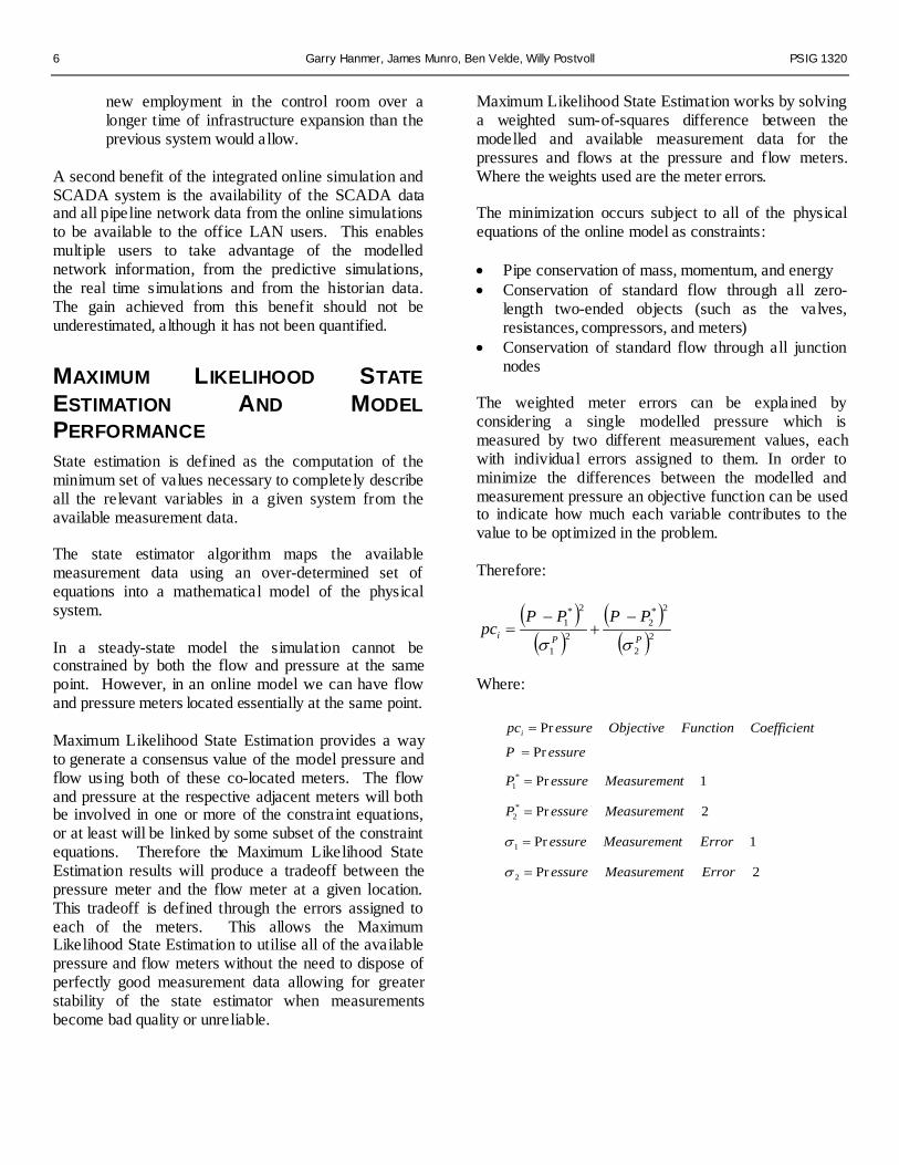
Introduction Pipelines are the fundamental structure by which hydrocarbon energy is transported. The safety, reliability and economic benefits of hydrocarbon energy transfer can be optimised through the use of pipeline simulation software. Online simulation software allows control room operators to operate and maintain complex pipeline networks while providing calibrated configurations for offline pipeline design studies and predictive simulation. Pipeline simulation software complements the full life cycle of a pipeline by considering the entire spectrum from the initial design studies to the pipeline operations and maintenance. 20% of the European natural gas consumption is exported through a complex pipeline network (see

PSIG 1320

Application Benefit of the Online Simulation Software for Gassco’s Subsea Pipeline Network Ben Velde, Willy Postvoll – Gassco Garry Hanmer, James Munro - ATMOS International Limited

2 Garry Hanmer, James Munro, Ben Velde, Willy Postvoll PSIG 1320

Figure 1 – Pipeline Network Schematic) of large diameter subsea pipelines between 300 km (190 miles) and 900 km (560 miles) long, with diameters up to 1.118 meter (44 inch). Approximately 100 billion standard cubic meters (3531.47 billion cubic feet) of Norwegian gas is transported within this pipeline network annually. Measurements are only available at the pipeline inlets and outlets above sea level, and therefore the state of the gas in these pipelines has to be calculated by pipeline simulation models. Consequently, these pipeline simulation models are essential when monitoring the operation of unmetered subsea and onshore locations in the network as well as performing predictive simulations for planned operational conditions and transport capacity calculations. The online simulation tool consists of 17 separate pipeline models which monitor the gas pipeline network as part of the Pipeline Management System (PMS). State estimation, using the maximum likelihood state estimator which utilises all of the available measurement data for flows and pressures provides an up to date calculation of the hydraulic and compositional properties of the gas in the pipeline network. Tuning algorithms for the pipeline efficiency tuning and flow meter offset tuning enhance the online simulation tool accuracy by utilising the long term behaviour of deviations between modelled and measurement values to automatically adjust system parameters so as to better match the measurement values. In addition to the online real time simulations, predictive modelling techniques that utilise a look-ahead (LAH) calculation engine can provide forecasts of pipeline conditions based on the current calculated state of the system and planned future shipper nominations.

CHARACTERISTICS – NEW/OLD PMS The SCADA system is of modern standard and was used as the framework for integrating the new pipeline model. The values and descriptions shown in ‘Table 1 – New and Old PMS Characteristics and Typical Settings’ are indicative as it may often be difficult to convert one method’s settings to another. The values also represent the users’ best practice in terms of accuracy versus performance. This is also hardware dependent from the period in use.

The comparison in ‘Table 1 – New and Old PMS Characteristics and Typical Settings’ shows some of the areas where the new system achieves benefits over the old system:

• Grid and Fluid Quality Resolution • Data validation • LAH duration and frequency • Nomination Vs frozen flow rates in LAH • Calibration methods • Information handling and display functionalities

NETWORK MODEL CALIBRATION Tuning of online network models to actual operational data is the key to achieving the required accuracy and reliability. The network model calibration is based on the sampling of the historian data of instrument measurements from the physical pipeline. Data sets where the flow is in a condition close to steady state can be extracted from the historian data. These data sets can be extracted for a full range of flow conditions, from zero flow to full capacity. The data is sampled through calibrated instruments on the network. Additional measurements and predictions for ambient sea bed temperature are used as well as the real gas temperature profile which is logged through the use of a scraper with a temperature sensor. The real instrument measurement data is then processed statistically and used as the basis for tuning the main pipeline in each network and then each branch roughness and heat transfer properties so that the simulation model hydraulics match those in the sampled data sets. This tuning may be automated using a tuning assistant tool embedded within the core simulation engine to make the tuning operation much more efficient. The tuning assistant aims to automate the iterative steps required when tuning pipeline properties such as pipe roughness and heat transfer. Utilising equal configurations for online and offline simulations allows the online model to effectively be used to calibrate the offline model and in turn optimize the accuracy of the offline simulations. This calibration is completed efficiently with no requirements to transfer tuned parameters between multiple configuration files, as the network model may

PSIG 1320 Application Benefit of the Online Simulation Software for Gassco’s Subsea Pipeline Netw ork 3

consist of a number of scenarios with individual set-points. These scenarios allow one configuration to have an online scenario and an offline capacity scenario for example. Once a configuration parameter such as the pipeline roughness or the heat transfer properties has been tuned, the tuned value is instantly available within all scenarios. The capacity scenario is run to verify that the expected simulation result is achieved to confirm all simulation settings are correct before undertaking major predictive work.

OPERATIONAL SCENARIOS The operational scenarios described below illustrate how the new pipeline management system contributes to increased sales, reduced costs, and reduced losses over what its predecessor contributed. These values have been identified and quantified by the online users in the Operations department in Gassco. The system developers, the authors and their colleagues in the Technology department have verified the correct unit price for each type of volumetric quantity has been applied. The overall network has an average delivery of 250 MMSCMD (8828.67 MMSCFD) for which the following gas unit prices have been applied: For rich gas volumes passing processing plants converting rich gas into dry gas and NGL, lost volumes have a unit price of USD 0.21 per Sm3 (USD 0.0036 per SCF). Redelivery later and net present value, as well as lost NGL at fields is accounted for. For other dry gas volumes, it is assumed these are delivered from swing fields where the lost volumes can be delivered during summertime at a reduced cost. The unit price for such volume loss is USD 0.069 per Sm3 (USD 0.0012 per SCF). Increased sales in winter lead to a corresponding cut in sales later (summer) to achieve the annual contractual agreed volume, so the same unit price also applies to losses.

BLENDING AND PEAK TRACKING Quality peak tracking on an individual component basis allows for the blending of off-specification fluids with on-specification fluids in order to meet the required delivery quality specifications within a pipeline network.

To blend the fluids efficiently the accurate prediction of the location of the off-specification gas quality peaks and the accurate forecasting of the throughput time of the gas quality peaks to the next possible mixing point are required. In order to successfully blend the gas at the subsea mixing points, the flow rates need to be controlled on the upstream boundary sources with consideration of the time lag to the subsea mixing point. A blending operation at a subsea mixing point due to off-specification gas may require one or more sources to reduce flow rate. This flow reduction results in lost profit during the blending operation which could typically last a few hours. Being able to accurately locate the position of the off-specification fluid allows the control room operator to minimise the amount of fluid to be held back for the blending operation.

• In handling CO2 or H2S blending of rich gas at a subsea mixing point for one of the 17 sub-models comprising the total network, it is estimated a reduction in held back gas of 15 MMSCMD (529.72 MMSCFD for 2 hours a day for 6 days a year due to improved system functionality and better quality tracking accuracy. This will result in 7.5 MSm3/year (264.86 MMSCF/year) reduced loss of rich gas production. As explained in the section on operational scenarios, rich gas is converted to dry gas and NGL for sale, and also impacts production of NGL at the delivering fields.

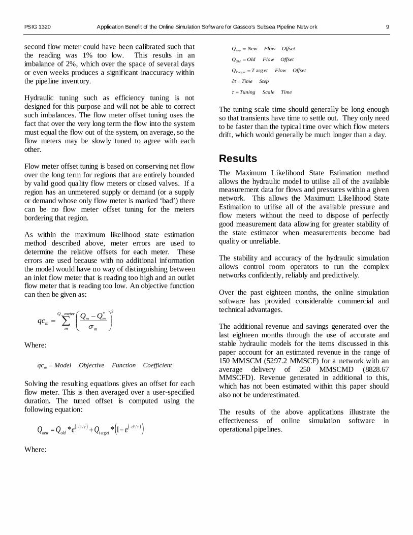
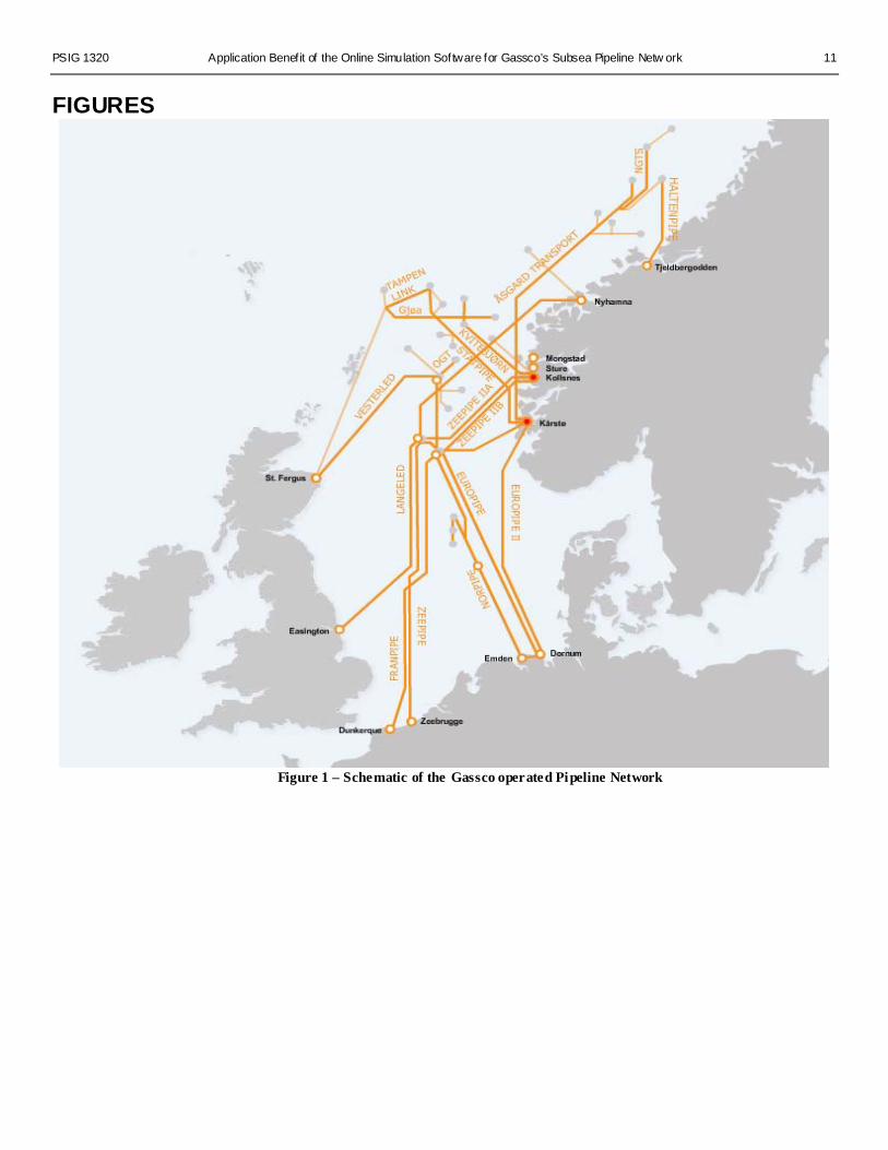
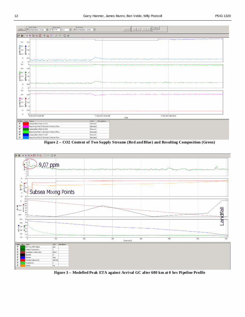
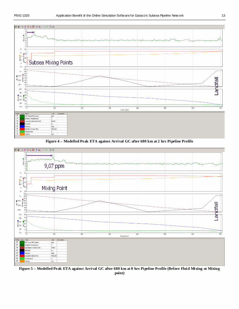
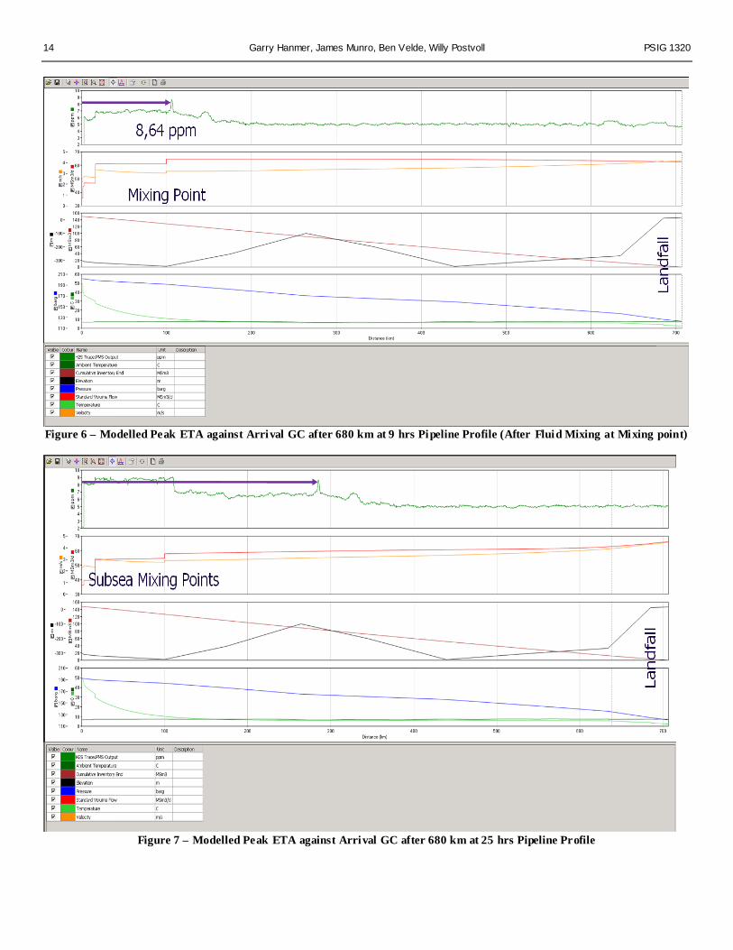
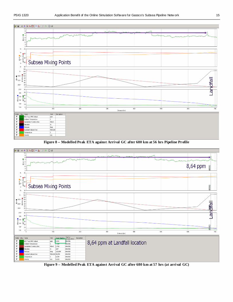
The blending of the off-specification gas with the on- specification gas is calculated within the model for each individual component of the gas composition and for specified trace elements and properties. This allows the composition to be estimated downstream of the mixing nodes where it is currently not viable to install compositional measurements. ‘Figure 2 shows the compositional content of Carbon Dioxide both before and after a mixing node. An upstream supply branch (red curve composition, pink curve flow rate) is mixed with a small branch supplying off specification gas (dark blue curve composition, light blue curve flow rate). The resulting composition downstream of the mixing node (dark green curve composition, light green curve flow rate) is calculated to be on-specification. Figures 3 to 10 illustrate the PMS tool for tracking a H2S peak towards the downstream subsea mixing points

4 Garry Hanmer, James Munro, Ben Velde, Willy Postvoll PSIG 1320

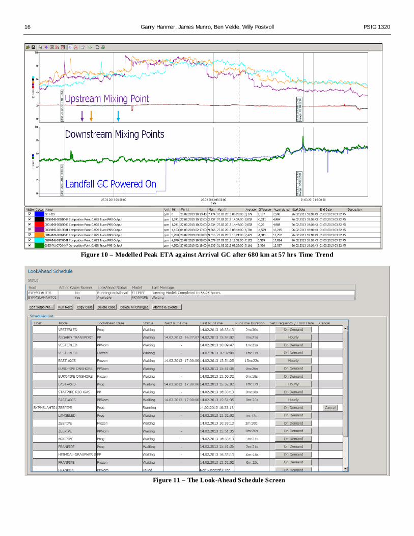
where blending may be possible. These figures illustrate how accurate the modelled peak tracking and modelled peak ETA can be when compared to the actual arrival gas as measured by a composition meter after approximately 680 km and 57 hrs of peak travel time. Figures 3 to 9 show the tracking of a H2S peak from the moment the peak enters the main pipeline, through a downstream mixing point and to the arrival gas composition meter at the outlet of the pipeline. The peak is calculated with an offset of less than 60 seconds at the arrival gas composition meter. ‘Figure 10 – Modelled Peak ETA against Arrival GC after 680 km at 57 hrs Time Trend’ shows a time based trend for a H2S peak. The chart at the top shows the H2S values at the upstream mixing point where the H2S peak enters the main line. The chart at the bottom shows the H2S measurement from the gas composition meter (blue) and the model calculated H2S (green) at the downstream pipeline outlet. The offset between H2S peaks as measured by composition meter and as calculated by model can be compared. For the example tracked peak there is an offset of less than 60 seconds which is negligible. Having such an accurate model prediction of ETA verifies that the model is calculating an accurate pipeline inventory and implies the model configuration parameters are set correctly. Having verified the online model configuration is accurate gives confidence in the model predictions for offline studies.

NOTIFICATION OF OFF-SPECIFICATION GAS The ability to accurately locate off-specification gas quality peaks which are located downstream of all of the mixing nodes is also vital information to the control room operator. This allows the shipper to be notified of the arrival of off-specification gas. The notifications are the basis of commercial discounts on the delivery of off- specification gas which are considerably less than the discount triggered by off specification gas delivered without notification.

• The estimated savings from accurate notification of the arrival of off-specification gas are currently not quantified, but should not be underestimated.

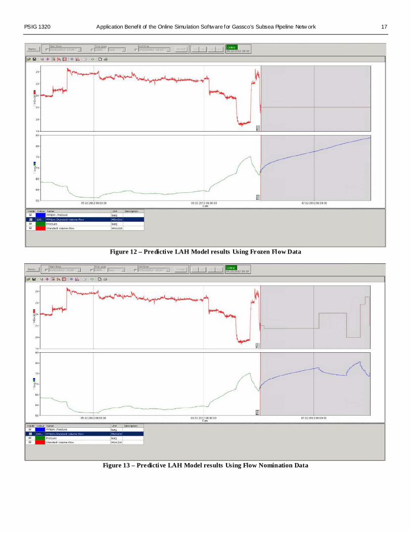
PREDICTIVE SIMULATION (LAH) Predictive simulation allows the control room operator to project the behaviour of the pipeline into the future based on the current pipeline conditions and the planned operations. This is conducted through a look-ahead (LAH) simulation engine which is run from the current pipeline conditions to a period within the future (typically 24 hours). These look-ahead simulations may be scheduled to automatically run periodically, for example every 30 minutes, or the look-ahead simulation may be manually launched on demand by the operator. ‘Figure 11 – The Look-Ahead Schedule Screen’ shows the Pipeline Management System’s look-ahead schedule screen as displayed in the SCADA. The look-ahead schedule screen allows the operator to schedule the running of each look-ahead case, set the frequency that the look-ahead cases will run and even edit the look-ahead case set-points. Shipper nominations from the Gas Management System are inputs into the predictive simulation as flow rate time series with variations in set-points. This is a significant advantage compared to running frozen set-points where the flow imbalance of the starting conditions is extrapolated into the future. The results from all of the predictive look-ahead simulations are instantly available to all of the pipeline operators through the integrated ‘Pipeline Management System’. ‘Figure 12 – Predictive Model Results Using Frozen Flow Data’ shows the historical and forecasted pipeline flow and pressure results for frozen flow data. ‘Figure 13 – Predictive Model Results Using Flow Nomination Data’ shows the historical and forecasted pipeline flow and pressure results following a scheduled look-ahead simulation, while utilising the nomination flows. The historical data is indicated with the white background, the current condition is labelled with a vertical line with label ‘Now’, and the forecasted look-ahead data is indicated with a grey background. All of this data is available within a single screen, allowing the operator to analyse all of the available data instantly. It is also possible to add historical metered data to such trend graphs, and each user can save their own custom

PSIG 1320 Application Benefit of the Online Simulation Software for Gassco’s Subsea Pipeline Netw ork 5

designed trends for quickly loading when needed. Utilising a production plan look-ahead case with future nominations allows the operator to fully utilise the pipeline’s capacity, without fear of inventory violations, Pressure Protection Shutdown and shortfalls of delivery.

• For many of the pipelines in the network the control room operators have been able to better control the linepack using the results from the LAH. This resulted in utilising 2 MMSCMD (70.63 MMSCFD) more for a period of 12 hrs over 60 days a year. This corresponds to 60 MMSCM/year (2118.88 MMSCF/year) of dry gas linked to swing field production.

Through an increase in accuracy of the online and the predictive look-ahead simulations, optimisation of short term sales is estimated to increase dry gas sales by 0.25 MMSCMD (8.83 MMSCFD), for 90 days a year for two of the pipelines supplying continental Europe.

• This results in 22.5 MMSCM (794.58 MMSCF) increased sale of dry gas linked to swing field production per year.

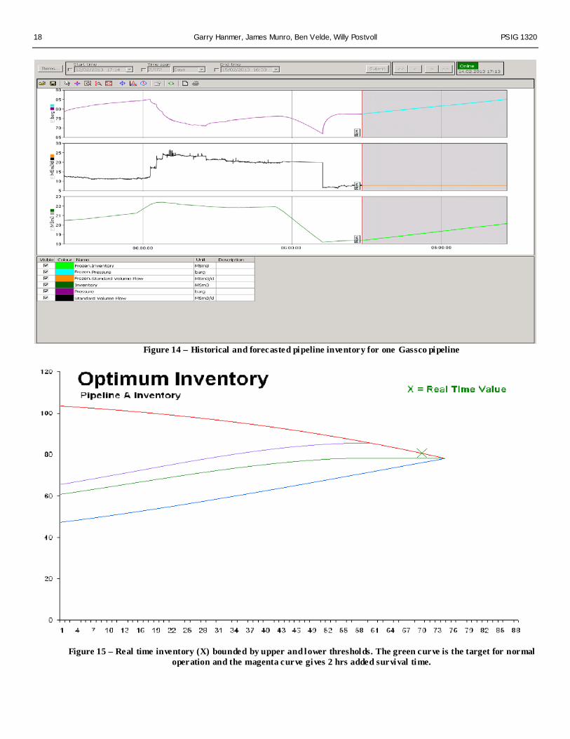
INVENTORY ANALYSIS Inventory is a paramount parameter used for hydrocarbon accounting in total mass, volume, and energy. Inventory may also be used for many other applications such as Estimated Time of Arrival (ETA), throughput time, and settle out pressure to name a few. Such calculations are available to the user from the online simulation without the requirements of manual calculations by the operators. ‘Figure 14 – Historical and Forecasted Pipeline Inventory for One Gassco Pipeline’ demonstrates the ability to combine data from the predictive simulations, the real time simulations and from the historian data. The accurate inventory calculations determine the available capacity and also contribute to the ETA accuracy, where accurate ETA allows for the tracking of off-specification gas. This knowledge allows the control room operator to have a more informed view of the pipeline conditions, and is often used as a basis for manual calculations.

For optimisation of transport fuel consumption as well as a minimum excess of linepack to handle sudden increase in nominations, “nose curve” type diagrams are used. An example is shown in ’Figure 15 – Real Time Inventory Bounded by Upper and Lower Thresholds’ where the real time inventory as calculated by the hydraulic model is indicated as a floating X inside the upper and lower inventory thresholds. The upper threshold is calculated using the hydraulic model with a fixed maximum pressure at the source, and the lower threshold with a fixed minimum pressure at the sink. The green curve represents a recommended condition with respect to both fuel consumption and operational flexibility under normal operation. This is the optimum position for where the X should be. The magenta curve gives 2 hrs additional survival time over the green curve. This is used during maintenance periods for example, when there may be fewer supplies available than normal and the consequences of a supply shutdown are more severe.

BALANCING PIPELINE PRESSURES On average twice a year the pressure level between two large pipelines are required to be balanced to blend off-specification gas through a cross over line. Due to the large inventory, pressure drop and slow response from the source to the sink, the operational procedures for balancing the pressure conditions are optimised using the look-ahead predictive simulation.

• It is estimated that accurate ETA and the look-ahead predictive simulation optimises this operation so that the holdback of rich gas on the upstream process plant is reduced by 5 MMSCMD (176.57 MMSCFD) for 3 hrs twice a year. This results in 1.25 MMSCM (44.14 MMSCF) increased sales a year.

INTEGRATED PMS As company infrastructure expands there is a corresponding increase in the information to be passed to control room operators. The integrated solution of online simulation and SCADA enables primary information from both systems to be clearly displayed to the control room operators, with secondary information only a click of a mouse away.

• Being able to obtain the critical information more efficiently has allowed Gassco to delay

6 Garry Hanmer, James Munro, Ben Velde, Willy Postvoll PSIG 1320

new employment in the control room over a longer time of infrastructure expansion than the previous system would allow.

A second benefit of the integrated online simulation and SCADA system is the availability of the SCADA data and all pipeline network data from the online simulations to be available to the office LAN users. This enables multiple users to take advantage of the modelled network information, from the predictive simulations, the real time simulations and from the historian data. The gain achieved from this benefit should not be underestimated, although it has not been quantified.

MAXIMUM LIKELIHOOD STATE ESTIMATION AND MODEL PERFORMANCE State estimation is defined as the computation of the minimum set of values necessary to completely describe all the relevant variables in a given system from the available measurement data. The state estimator algorithm maps the available measurement data using an over-determined set of equations into a mathematical model of the physical system. In a steady-state model the simulation cannot be constrained by both the flow and pressure at the same point. However, in an online model we can have flow and pressure meters located essentially at the same point. Maximum Likelihood State Estimation provides a way to generate a consensus value of the model pressure and flow using both of these co-located meters. The flow and pressure at the respective adjacent meters will both be involved in one or more of the constraint equations, or at least will be linked by some subset of the constraint equations. Therefore the Maximum Likelihood State Estimation results will produce a tradeoff between the pressure meter and the flow meter at a given location. This tradeoff is defined through the errors assigned to each of the meters. This allows the Maximum Likelihood State Estimation to utilise all of the available pressure and flow meters without the need to dispose of perfectly good measurement data allowing for greater stability of the state estimator when measurements become bad quality or unreliable.

Maximum Likelihood State Estimation works by solving a weighted sum-of-squares difference between the modelled and available measurement data for the pressures and flows at the pressure and flow meters. Where the weights used are the meter errors. The minimization occurs subject to all of the physical equations of the online model as constraints: • Pipe conservation of mass, momentum, and energy • Conservation of standard flow through all zero-

length two-ended objects (such as the valves, resistances, compressors, and meters)

• Conservation of standard flow through all junction nodes

The weighted meter errors can be explained by considering a single modelled pressure which is measured by two different measurement values, each with individual errors assigned to them. In order to minimize the differences between the modelled and measurement pressure an objective function can be used to indicate how much each variable contributes to the value to be optimized in the problem. Therefore:

Where:

( )( )

( )( )22

2*2

21

2*1

PPi

PPPPpc

σσ

−+

−=

2Pr

1Pr

2Pr

1Pr

Pr

Pr

2

1

*2

*1

ErrortMeasuremenessure

ErrortMeasuremenessure

tMeasuremenessureP

tMeasuremenessureP

essureP

tCoefficienFunctionObjectiveessurepci

=

=

=

=

=

=

σ

σ

PSIG 1320 Application Benefit of the Online Simulation Software for Gassco’s Subsea Pipeline Netw ork 7

For the independent pressure variable, this becomes:

Where:

Therefore if the errors on the two meters are equal, then the Maximum Likelihood State Estimation solution will be the average of the two pressure measurements, however if the errors on the two meters are significantly different then the Maximum Likelihood State Estimation solution will be closer to the meter with the smallest error. For example:

Then:

Maximum Likelihood State Estimation weights the results towards the better meter. If we assume that the meter errors are normally distributed, the Maximum Likelihood State Estimation result produces the most likely estimate of the state of the actual pressure value. Similarly this can be applied to the flow meters. Now consider a model section with N pressures and flows and M model equations. The Maximum Likelihood State Estimation treats the M model equations as constraints on an optimization problem that minimizes the differences between the metered values

and the modelled values. The model objective function coefficient then becomes:

Where:

The objective function coefficient for the model is then minimized by its derivative with respect to the independent pressure and flow variables, and all of the other pressures, flows, and temperatures involved in the model equations to be equal to zero:

The online model may then solve a set of simultaneous equations exactly as it does within the offline model, where many of the equations are identical. The full set of equations is nonlinear, so the online simulation may then linearise them in the same way the offline simulation does. The Maximum Likelihood State Estimator may then utilise all of the available measurement data while weighting towards the meters which are the most accurate meters, allowing the state estimator to provide an accurate solution and providing greater stability in the event where measurements become bad quality or unreliable.

( )( )

( )( )

( ) ( ) ( ) ( )

( ) *2

*1

22

*2

21

*1

22

21

22

*2

21

*1

1

1

11

022

0

PPP

PPP

PPPP

Pc

PPPP

PP

i

αα

σσσσ

σσ

−+=

+=

+

=−

+−

=∂∂

( )( ) ( )22

21

22

PP

P

σσσα+

=

PP12 *100 σσ =

*2

*1 101

1101100 PPP +=

{ }( )( )∑

∑∑ +

−+

−=

eqnel

mmmmm

meterQ

m m

mmmeterP

m m

mmm

QPf

QQPPmc

_mod

_ 2*_ 2*

,λ

σσ

EquationsModel

ErrortMeasuremen

tMeasuremenFlowQ

FlowQ

tCoefficienFunctionObjectiveModelmc

m

m

m

m

m

=

=

=

=

=

λ

σ 1

1*

0

0

0

=∂∂

=∂∂

=∂∂

m

m

m

m

m

m

cQcPc

λ

8 Garry Hanmer, James Munro, Ben Velde, Willy Postvoll PSIG 1320

EFFICIENCY TUNING In addition to the user initiated automatic offline tuning which is conducted with the aid of the tuning assistant, the online model also performs continuous tuning. This continuous tuning is conducted to take into account changes within the pipeline roughness, meter drift, and unknown ambient conditions such as currents or unknown seabed temperatures for example. Hydraulic tuning is driven by the differences between the measured and modelled values of pressure and flow at the pressure and flow meters. The model pressures and flows obey all of the physical laws everywhere in the pipeline, but represent a compromise between the flow and pressure meters bounding the system. Thus at each pressure meter there is a pressure discrepancy between the modelled and measured pressure, and at each flow meter there is a corresponding flow discrepancy. The pressure and flow discrepancies for each pipe are then used to compute the efficiency that in steady state would produce the observed measurement pressures and flows. For each region bounded by pressure and flow meters, a volume-weighted average efficiency is calculated and updated. If there is sufficient flow to produce a tuneable pressure drop, some fraction of this efficiency update is then applied to each pipe in the region, depending on the time step and the tuning rate specified for that pipe. The pipe efficiency is a factor used to multiply the frictional pressure drop as follows:

Where:

The efficiency tuning process calculates for each pipe a target efficiency which is the efficiency that would give the best match between the modeled and measured pressures and flows currently if the line was in steady state. The model then adjusts the tuned efficiency, which is the efficiency actually used by the model towards the target efficiency according to the equation:

Where:

The efficiency tuning scale time should generally be set to longer than the time it takes a hydraulic transient to settle down. This tuning method was observed to work regardless of time step length, automatically producing stable results even if the tuning scale time is very short. In an online model it would be expected that will typically be much less than , and so this will be equivalent to adding a fraction of – that is just / . Efficiency tuning is active for any group of pipes with good-quality pressure and flow meters at both the upstream and downstream ends, as long as the frictional pressure drop in those pipes is not below a threshold that corresponds to nearly-stopped flow. These thresholds exist because as the frictional losses drop, the ability of the model to adjust the overall pressure drop by changing the tuned efficiency also drops. The tuned efficiency may also be capped to a range with a maximum and minimum limit to regulate the tuned efficiency during small flow rates where tuning may still be active.

FLOW METER OFFSET TUNING Over extended periods no pipeline section can keep packing or unpacking indefinitely. This means that the total flow into any subsection of the pipeline must average to zero, if we average over a long enough time. Long term imbalances are often the result of flow meter inaccuracy. These imbalances and inaccuracies occur even in calibrated instrumentation. If two flow meters are considered for example, where each flow meter has been calibrated to an accuracy of 1%. In the extreme case one meter could have been calibrated such that the reading was 1% too high, and the

2_ / Eff BasePdPd =

EfficiencyE

DropessureFrictionalBasef

DropessureFrictionalf

BasePd

Pd

=

=

=

Pr

Pr

_

( ) ( )( )ττ /arg

/ 1** tett

toldnew eEeEE −∂−∂ −+=

7.2

argarg

=

=

=∂

=

=

=

e

TimeScaleTuning

StepTimet

EfficiencyetTE

EfficiencyOldE

EfficiencyNewE

etT

Old

new

τ

t∂τ

OldE etTE arg

t∂ τ

PSIG 1320 Application Benefit of the Online Simulation Software for Gassco’s Subsea Pipeline Netw ork 9

second flow meter could have been calibrated such that the reading was 1% too low. This results in an imbalance of 2%, which over the space of several days or even weeks produces a significant inaccuracy within the pipeline inventory. Hydraulic tuning such as efficiency tuning is not designed for this purpose and will not be able to correct such imbalances. The flow meter offset tuning uses the fact that over the very long term the flow into the system must equal the flow out of the system, on average, so the flow meters may be slowly tuned to agree with each other. Flow meter offset tuning is based on conserving net flow over the long term for regions that are entirely bounded by valid good quality flow meters or closed valves. If a region has an unmetered supply or demand (or a supply or demand whose only flow meter is marked ‘bad’) there can be no flow meter offset tuning for the meters bordering that region. As within the maximum likelihood state estimation method described above, meter errors are used to determine the relative offsets for each meter. These errors are used because with no additional information the model would have no way of distinguishing between an inlet flow meter that is reading too high and an outlet flow meter that is reading too low. An objective function can then be given as:

Where:

Solving the resulting equations gives an offset for each flow meter. This is then averaged over a user-specified duration. The tuned offset is computed using the following equation:

Where:

The tuning scale time should generally be long enough so that transients have time to settle out. They only need to be faster than the typical time over which flow meters drift, which would generally be much longer than a day.

Results The Maximum Likelihood State Estimation method allows the hydraulic model to utilise all of the available measurement data for flows and pressures within a given network. This allows the Maximum Likelihood State Estimation to utilise all of the available pressure and flow meters without the need to dispose of perfectly good measurement data allowing for greater stability of the state estimator when measurements become bad quality or unreliable. The stability and accuracy of the hydraulic simulation allows control room operators to run the complex networks confidently, reliably and predictively. Over the past eighteen months, the online simulation software has provided considerable commercial and technical advantages. The additional revenue and savings generated over the last eighteen months through the use of accurate and stable hydraulic models for the items discussed in this paper account for an estimated revenue in the range of 150 MMSCM (5297.2 MMSCF) for a network with an average delivery of 250 MMSCMD (8828.67 MMSCFD). Revenue generated in additional to this, which has not been estimated within this paper should also not be underestimated. The results of the above applications illustrate the effectiveness of online simulation software in operational pipelines.

∑

−=

meterQ

m m

mmm

QQqc_ 2*

σ

tCoefficienFunctionObjectiveModelqcm =

( ) ( )( )ττ /arg

/ 1** tett

toldnew eQeQQ −∂−∂ −+=

TimeScaleTuning

StepTimet

OffsetFlowetTQ

OffsetFlowOldQ

OffsetFlowNewQ

etT

Old

new

=

=∂

=

=

=

τ

argarg

10 Garry Hanmer, James Munro, Ben Velde, Willy Postvoll PSIG 1320

Conclusions The discussed benefits of the online hydraulic simulation software and integration in SCADA have made the Pipeline Management System an essential tool for Gassco to manage the daily operations and maintenance of the largest sub-sea pipeline network in the world. The increased model accuracy gained through the use of the Maximum Likelihood State Estimator and the online and offline tuning functionalities allow the control room operator to benefit from increased utilisation of the pipeline’s current and future capacity. This paper has demonstrated some of the benefits of online simulation software when utilised as a tool to assist operational decision making. The costs benefit analysis of a few annual operational scenarios described above sums to USD 7.5 Million per year.

References 1. Tuning of Subsea Pipeline Models to Optimize

Simulation Accuracy, (Pipeline Simulation Interest Group, May 15-18 2012, Santa Fe, New Mexico). Garry Hanmer, et al.

2. Maximum Likelihood Approach to State Estimation in Online Pipeline Models, (International Pipeline Conference, Sep 24-28 2012, Calgary, Canada) Jason Modisette

3. Online Application of Hydraulic Simulation Software to Gassco’s Subsea Pipeline Network, (International Pipeline Conference, Sep 24-28 2012, Calgary, Canada). Eadred Birchenough, et al.

4. State Estimate in Online Models, (Pipeline Simulation Interest Group, May 12-15 2009, Galveston, Texas). Jason Modisette,

5. Pipeline Design and Construction – A Practical Approach. M. Mohitpour, H. Golshan, A. Murray.

PSIG 1320 Application Benefit of the Online Simulation Software for Gassco’s Subsea Pipeline Netw ork 11

FIGURES

Figure 1 – Schematic of the Gassco operated Pipeline Network

12 Garry Hanmer, James Munro, Ben Velde, Willy Postvoll PSIG 1320

Figure 2 – CO2 Content of Two Supply Streams (Red and Blue) and Resulting Composition (Green)

Figure 3 – Modelled Peak ETA against Arrival GC after 680 km at 0 hrs Pipeline Profile

PSIG 1320 Application Benefit of the Online Simulation Software for Gassco’s Subsea Pipeline Netw ork 13

Figure 4 – Modelled Peak ETA against Arrival GC after 680 km at 2 hrs Pipeline Profile

Figure 5 – Modelled Peak ETA against Arrival GC after 680 km at 8 hrs Pipeline Profile (Before Fluid Mixing at Mixing

point)

14 Garry Hanmer, James Munro, Ben Velde, Willy Postvoll PSIG 1320

Figure 6 – Modelled Peak ETA against Arrival GC after 680 km at 9 hrs Pipeline Profile (After Fluid Mixing at Mixing point)

Figure 7 – Modelled Peak ETA against Arrival GC after 680 km at 25 hrs Pipeline Profile

PSIG 1320 Application Benefit of the Online Simulation Software for Gassco’s Subsea Pipeline Netw ork 15

Figure 8 – Modelled Peak ETA against Arrival GC after 680 km at 56 hrs Pipeline Profile

Figure 9 – Modelled Peak ETA against Arrival GC after 680 km at 57 hrs (at arrival GC)

16 Garry Hanmer, James Munro, Ben Velde, Willy Postvoll PSIG 1320

Figure 10 – Modelled Peak ETA against Arrival GC after 680 km at 57 hrs Time Trend

Figure 11 – The Look-Ahead Schedule Screen

PSIG 1320 Application Benefit of the Online Simulation Software for Gassco’s Subsea Pipeline Netw ork 17

Figure 12 – Predictive LAH Model results Using Frozen Flow Data

Figure 13 – Predictive LAH Model results Using Flow Nomination Data

18 Garry Hanmer, James Munro, Ben Velde, Willy Postvoll PSIG 1320

Figure 14 – Historical and forecasted pipeline inventory for one Gassco pipeline

Figure 15 – Real time inventory (X) bounded by upper and lower thresholds. The green curve is the target for normal

operation and the magenta curve gives 2 hrs added survival time.

PSIG 1320 Application Benefit of the Online Simulation Software for Gassco’s Subsea Pipeline Netw ork 19

TABLES

Table 1 – New and Old PMS Characteristics and Typical Settings

newPMS old PMSDeveloped & In-Use period 2011-2013 1992-2009Grid resolution* Adaptive from 1 m 800 - 10 000 mFluid batch resolution* 500 - 1000 m 800 - 20 000 mTime step, RTM 60 sec 60 secNetwork models, single phase gas 17 + (3 of 17 combined for longer peak routes) 17Data Validation Overview Sortable list in GUI - Focus on critical signal status Unsorted list for maintenance not for operation Restart - Edit inputs Advanced Graphical Editor - easy to use Graphical Editor - seldom usedLAH duration - normal scenario 24 hrs 4 hrsLAH frequency - normal scenario 15 min 60 minLAH control mode setpoint Shipper's Nominations Flow mode Frozen RTM Flow modeLAH AdHoc simulation On demand - Frequently used On demand - Rarely usedFriction tuning method Maximum Likelihood State Estimation Equal Error FractionTemperature tuning method Heat Transfer of last sections tuned to sink T-Meter Whole T-amb profile tuned to sink T-meterPeak Travel Time tuning method (ETA) Inventory tuned by Heat Transfer -Ambient Temperature method UK Met Daily / Statistical Monthly 2012 /Fixed UK Met Daily / Statistical Monthly 2009 /FixedOnline GUI Full Integration in SCADA Framework/Navigation StandaloneTrend & Profile - curve peaks Always visible Appearing/Disappearing Trend module - combinations of input Historian/SCADA/RTM/LAH SCADA/RTM/LAHProfile module - time step selection Historic/Current/Future Current/FutureStatistics Legend Grid Trend & Profile -Peak List Auto Triggered Peaks, LAH based ETA, more details BasicInventory reports Scheduled, On demand Scheduled* not directly comparable

RTM Model Characteristics & Typical Settings

Feature